NISTIR 89-4035 new NIST PUBLICATION June 12, 1989 Considerations of Stack Effect in Building Fires John H. Klote U.S. DEPARTMENT OF COMMERCE National Institute of Standards and Technology National Engineering Laboratory Center for Fire Research Gaithersburg, MD 20899 January 1989 Issued May 1989 Sponsored by; U.S. Fire Administration Emmitsburg, MD 21727
Transcript
NISTIR 89-4035new NIST PUBLICATION
June 12, 1989
Considerations of StackEffect in Building Fires
John H. Klote
U.S. DEPARTMENT OF COMMERCENational Institute of Standards and Technology
National Engineering Laboratory
Center for Fire Research
Gaithersburg, MD 20899
January 1989
Issued May 1989
Sponsored by;
U.S. Fire Administration
Emmitsburg, MD 21727
NISTIR 89-4035
Considerations of StackEffect in Building Fires
John H. Klote
U.S. DEPARTMENT OF COMMERCENational Institute of Standards and Technology
National Engineering Laboratory
Center for Fire Research
Gaithersburg, MD 20899
January 1989
Issued May 1989
National Bureau of Standards became the
National Institute of Standards and Technology
on August 23, 1988, when the Omnibus Trade and
Competitiveness Act was signed. NIST retains
all NBS functions. Its new programs will encourage
improved use of technology by U.S. industry.
Sponsored by;
U.S. Fire Administration
Emmitsburg, MD 21727
U.S. DEPARTMENT OF COMMERCERobert Mosbacher, Secretary
NATIONAL INSTITUTE OF STANDARDSAND TECHNOLOGYRaymond G. Kammer, Acting Director
TABLE OF CONTENTS
LIST OF FIGURES v
LIST OF TABLES viii
Abstract 1
1. INTRODUCTION 2
2. DRIVING FORCES OF SMOKE MOVEMENT 2
2.1 Stack Effect 3
2.2 Buoyancy of Combustion Gases 11
2.3 Expansion of Combustion Gases 12
2.4 Wind Effect 13
2.5 Ventilation Systems 16
2.6 Elevator Piston Effect 17
3. LOCATION OF NEUTRAL PLANE 22
3.1 Shaft with a Continuous Opening 22
3.2 Shaft With Two Vents 24
3.3 Vented Shaft 26
4. FRICTION LOSS IN SHAFTS 28
5. STEADY SMOKE CONCENTRATIONS 30
6. NETWORK MODELS 31
6.1 Network Model Concept 32
6.2 Mass Flow Rates 32
6.3 Unsteady Smoke Concentrations 34
6.4 Unsteady Temperatures 36
7. ZONE MODELS 36
7.1 Compartment Fire Phenomena 37
7.2 Application to High Rise Buildings 41
8. STEADY FLOW NETWORK CALCULATIONS 47
8.1 Building with Doors Closed and No Vents (Case 1) 50
8.2 Top Vented Elevator Shaft (Case 2) 57
8.3 Top Vented Stair Shaft (Case 3) 58
8.4 Top Vents on Stair and Elevator Shafts (Case 4) 59
8.5 Top and Bottom Vented Stair Shaft (Case 5) 59
8.6 Bottom Vented Stair Shaft (Case 6) 60
8.7 Effect of Elevated Temperatures (Cases 4A and 6A) 61
8.8 Fire Above the Neutral Planes 62
iii
TABLE OF CONTENTS Continued
9. FUTURE EFFORT 67
9.1 Full Scale Experiments 68
9.2 Scale Model Experiments 69
10. CONCLUSIONS 69
11. ACKNOWLEDGMENTS 71
12. NOMENCLATURE 71
13. REFERENCES 72
IV
LIST OF FIGURES
Figure 1. Air movement due to normal and reverse stack effect 4
Figure 3. Comparison of measured and calculated pressure differencesacross the outside wall of the Canadian Fire ResearchTower for different outside temperatures 9
Figure 4. Comparison of measured and calculated pressure differencesacross a shaft enclosure of the Canadian Fire ResearchTower for different building leakages 10
Figure 5. Pressures occurring during a fully involved compartment fire . 11
Figure 6. Wind velocity profiles for flat and very rough terrain .... 16
Figure 7 . Airflow due to downward movement of elevator car 18
Figure 8. Pressure difference, AP^^ ,
across elevator lobby of a
Toronto hotel due to piston effect 20
Figure 9. Calculated upper limit of the pressure difference, (APj^^)^,
from the elevator lobby to the building due to pistoneffect 21
Figure 10. Normal stack effect between a single shaft connected to
the outside by a continuous opening 22
Figure 11. Stack effect for a shaft with two openings 24
Figure 13. Stratified smoke flow as simulated by zone fire models .... 37
Figure 14. Smoke flow at 0.5 minutes after ignition in a ten storybuilding calculated by a zone model 42
Figure 15. Smoke flow at 1.0 minutes after ignition in a ten story
building calculated by a zone model A3
Figure 16. Smoke flow at 3.0 minutes after ignition in a ten story
building calculated by a zone model A4
Figure 17. Smoke flow at 4.5 minutes after ignition in a ten story
building calculated by a zone model 45
V
LIST OF FIGURES Contents
Figure 18. Floor plan of building used for example analyses 48
Figure 19. Calculated smoke concentrations due to a fourth floorfire in a 20 story building without any vents or opendoors (Case 1) 51
Figure 20. Calculated smoke concentrations due to a fourth floorfire in a 20 story building with a top vented elevatorshaft (Case 2) 52
Figure 21. Calculated smoke concentrations due to a fourth floorfire in a 20 story building with a top vented stairwell(Case 3) 53
Figure 22. Calculated smoke concentrations due to a fourth floorfire in a 20 story building with top vents in elevatorand stair shafts (Case 4) 54
Figure 23. Calculated smoke concentrations due to a fourth floorfire in a 20 story with top vents in elevator and stairshafts and an open stair door (Case 5) 55
Figure 24. Calculated smoke concentrations due to a fourth floorfire in a 20 story building with top vents in elevatorand stairwell shafts and with an open stairwell door(Case 6) 56
Figure 25. Pressures for a building with a top vented shaft 58
Figure 26. Pressures for a building with a shaft vented at the top
and bottom 60
Figure 27. Pressures for a building with a bottom vented shaft 61
Figure 28. Calculated smoke concentrations due to a fourth floorfire in a 20 story building with top vents in elevatorand stairwell shafts and with elevated shaft temperatures(Case 4A) 63
Figure 29. Calculated smoke concentrations due to a fourth floor
fire in a 20 story building with a top vented elevator,
with an open stairwell door, and with elevated shaft
temperatures (Case 6A) 64
VI
LIST OF FIGDRES Contents
Figure 30. Calculated smoke concentrations due to a fifteenth floorfire in a 20 story building with a top vented elevatorshaft (Modification of case 2) 65
Figure 31. Calculated smoke concentrations due to a fifteenth floorfire in a 20 story building with a top vented stairwell(Modification of case 3) 66
vii
LIST OF TABLES
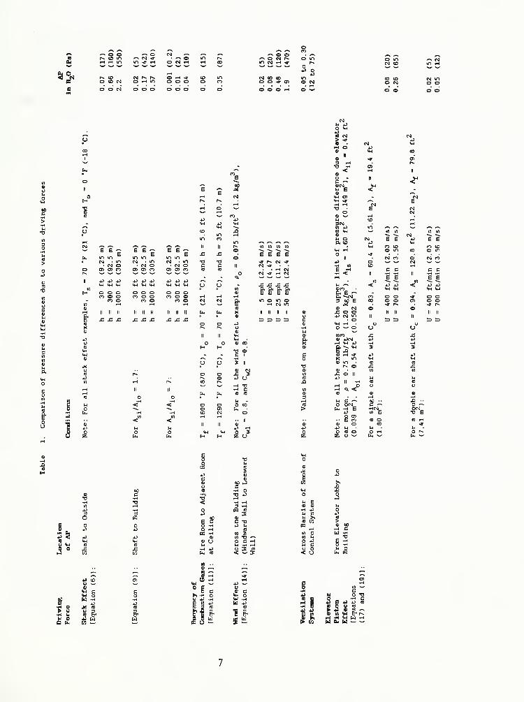
Table 1. Comparison of pressure differences due to various drivingforces 7
Table 2. Average pressure coefficients for walls of rectangularbuildings 14
Table 3. Dimensions used for Tanaka's (1983) zone modelsimulation of smoke movement in a ten story building 41
Table 4. Flow areas and other data about building for example analyses 47
Table 5. List of vent and door conditions for example analyses .... 50
Table 6. Calculated flow rates (Ib/min) in a building without anyvents or open doors (Case 1) 76
Table 7. Calculated flow rates (Ib/min) in a building with a topvented elevator shaft (Case 2) 77
Table 8. Calculated flow rates (Ib/min) in a building with a topvented stairwell (Case 3) 78
Table 9. Calculated flow rates (Ib/min) in a building with a topvented elevator shaft and a top vented stairwell (Case 4) . . 79
Table 10. Calculated flow rates (Ib/min) in a building with a top
vented elevator shaft and a stairwell with a top ventand an open exterior door (Case 5) 80
Table 11. Calculated flow rates (Ib/min) in a building with a topvented elevator shaft and a stairwell with an open exteriordoor (Case 6) 81
Table 12. Calculated flow rates (Ib/min) in a building with top
vented elevator shaft and stairwell and with elevatedshaft and fire floor temperatures (Case 4A) 82
Table 13. Calculated flow rates (Ib/min) in a building with a top
vented elevator shaft, with a stairwell with an openexterior door, and with elevated shaft and fire floor
temperatures (Case 6A)
viii
83
CONSIDERATIONS OF STACK EFFECT IN BUILDING FIRES
John H. Klote
Abstract
The following driving forces of smoke movement in buildings are
discussed: stack effect, buoyancy of combustion gases, expansion of combustion
gases, wind effect, and elevator piston effect. Based on an analysis of
elevator piston effect, it is concluded that the likelihood of smoke being
pulled into an elevator shaft due to elevator car motion is greater for single
car shafts than for multiple car shafts. Methods of evaluating the location
of the neutral plane are presented. It is shown that the neutral plane
between a vented shaft and the outside is located between the neutral plane
height for an unvented shaft [equation (23)] and the vent elevation.
Calculations are presented that show that pressure losses due to friction are
generally negligible for unvented shafts with all doors closed. The
capabilities and limitations of network models and zone models are discussed.
The network method was applied to several cases of open and closed doors and
shaft vents likely to occur during firefighting. For the cases evaluated,
shaft venting did not result in any significant reduction in smoke
concentrations on the floors of the building. One of the cases showed that
for low outside temperatures, bottom venting of a shaft can result in shaft
pressurization. Other cases demonstrated that elevated temperatures of
combustion gases can result in downward smoke flow from one floor to another.
Much of the information in this paper is applicable to the migration of other
airborne matter such as hazardous gases and bacteriological or radioactive
In building fires, smoke often migrates to locations remote from the
fire space. Stairwells and elevator shafts frequently become smoke -logged,
thereby blocking evacuation and inhibiting fire fighting. In this paper
several of the driving forces of smoke movement are discussed. The steady
flow analysis of stack effect and some considerations of unsteady flow are
addressed. The steady flow methods are applied to situations of open doors
and shaft vents likely to occur during firefighting. A number of
generalizations which could be of use to fire fighters are presented. The
information in this paper also is applicable to the migration of other
airborne matter such as hazardous gases, bacteriological matter or radioactive
matter in laboratories, hospitals, or industrial facilities. However, the
discussion in this paper is primarily aimed at smoke movement.
This paper does not address the pressurization approach to the smoke
movement problem. This approach is referred to as smoke control and is
addressed in the National Fire Protection Association (NFPA) recommended
practice 92A (1988) and the American Society of Heating, Refrigerating and Air
ASHRAE Smoke Control Manual (Klote and Fothergill 1983)
.
In this paper the term smoke is used in accordance with the NFPA 92A
(NFPA 1988) definition which states that smoke consists of the airborne solid
and liquid particulates and gases evolved when a material undergoes pyrolysis
or combustion, together with the quantity of air that is entrained or
otherwise mixed into the mass
.
2. DRIVING FORCES OF SMOKE MOVEMENT
The driving forces of smoke movement include naturally occurring stack
effect, buoyancy of combustion gases, expansion of combustion gases, the wind
effect, fan powered ventilation systems, and elevator piston effect. This
report discusses these driving forces, and in particular addresses smoke
2
movement due to the stack effect process, either naturally occurring or that
of combustion gases. Stack effect is discussed here as acting alone in order
to facilitate discussion and analysis. While other driving forces may act in
conjunction with stack effect, there are cases where stack effect is the
dominate driving force. Consideration of stack effect acting in the absence
of other driving forces can lead to an understanding of smoke transport for
these cases.
2 . 1 Stack Effect
Frequently when it is cold outside, there is an upward movement of air
within building shafts, such as stairwells, elevator shafts, dumbwaiters
shafts, mechanical shafts, and mail chutes. Air in the building has a buoyant
force because it is warmer and therefore less dense than outside air. The
buoyant force causes air to rise within building shafts. This phenomenon is
called by various names such as stack effect, stack action, and chimney
effect. These names come from the comparison with the upward flow of gases in
a smoke stack or chimney. However, a downward flow of air can occur in air
conditioned buildings when it is hot outside. For this paper, the upward flow
will be called normal stack effect, and the downward flow will be called
reverse stack effect as illustrated in figure 1.
Most building shafts have relatively large cross sectional areas, and
for most flows typical of those induced by stack effect the friction losses
are negligible in comparison with pressure differences due to buoyancy.
Accordingly, this analysis is for negligible shaft friction, but shaft
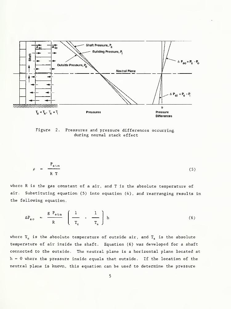
friction is specifically addressed later. Pressure, ,within a shaft is due
to fluid static forces and can be expressed as
where g is the acceleration of gravity, z is elevation, and is gas density
inside the shaft. For the elevations relevant to buildings, the acceleration
of gravity can be considered constant. For constant density, equation (1) can
be integrated from z = 0 to z = h to yield
3
Normal Stack Effect Reverse Stack Effect
Note: Arrows Indicate Direction of Air Movement
Figure 1. Air movement due to normal and reverse stack effect
Ps = Pa - Ps g h (2)
where is the pressure at h = 0. To simplify the analysis, the vertical
coordinate system is selected such that at h = 0. In the absence of
wind effects, the outside pressure, P^,
is
Po = Pa - g h (3)
where is the density outside the shaft. Pressures inside the shaft and
outside the building are graphically illustrated in figure 2 for normal stack
effect. This figure also shows the pressure of the building spaces, and
methods of calculating this are presented later in this section. The pressure
difference, AP^^, from the inside to the outside is expressed as
- P. - - <>.) g h W
Because variations in pressure within a building are very small compared
to atmospheric pressure, atmospheric pressure, Patm’ used in
calculating gas density, p, from the ideal gas equation.
4
Figure 2. Pressures and pressure differences occurringduring normal stack effect
patmP = (5)
R T
where R is the gas constant of a air, and T is the absolute temperature of
air. Substituting equation (5) into equation (4), and rearranging results in
the following equation.
APS O
g Patm( 6 )
where is the absolute temperature of outside air, and is the absolute
temperature of air inside the shaft. Equation (6) was developed for a shaft
connected to the outside. The neutral plane is a horizontal plane located at
h = 0 where the pressure inside equals that outside. If the location of the
neutral plane is known, this equation can be used to determine the pressure
5
difference from the inside to the outside regardless of variations in building
leakage or the presence of other shafts.
For example, if the neutral plane is located at the mid height of a 600
ft (185 m) tall building^ with inside and outside temperatures of 70 "F (21 C)
and 0 °F (-18 C),pressure difference due to stack effect is .66 in H
2O (164
Pa) at the top of the shaft. Methods of determining the location of the
neutral plane are discussed later. Table 1 is a comparison of pressure
differences due to various driving forces.
The concept of the effective flow area can be used to evaluate the
pressure,,on the floor. The effective area of a system of flow areas is
the area that results in the same flow as the system when it is subjected to
the same pressure difference over the total system of flow paths. Readers are
referred to Klote and Fothergill (1983) for a detailed discussion of effective
flow areas. In general, for flow areas,,in series where i is from 1 to n,
the effective area,,
is
Ae ( 7 )
This relation assumes that the flows can only occur in one direction at
any flow path and that the air temperatures in the paths are the same . For
the system of flow paths illustrated in figure 2, the effective flow area per
floor is
( 8 )
where A^^
is the per floor area between the shaft and the building, and A^ is
the per floor area between the building and the outside. The mass flow rate,
^This means that h = 300 ft (92.5 m) at the top of the building.
6
^ <0
^Ss
^ o^ o«n csj
O O <9* O)
O O O rH
o mps.
o^ o•no Cv]
0)
4J ^o ^2 O
evj
E -r
6
M E
»n ^ ^
o o o
E £
o o orj o o
II II H
^ j: X
E E
o o o
II II II
XXX
M (A V) M
^ ^ ^ 'e
•9- <NJ
CM ^• • »H CM
CM -«T «-• CM
X X X X§• t i tvn o un o
iH CM mII tl It II
2 2 3 2
$ II
+3 O
tt>CO
6 E --Cu7 OO E
0) CMX O O
O 4J(M^ ^i':Q'"® ft -9-
K® U-J oOX o
11
u c ^O OCM_U< -H E
E ECO {£>
c c
E E
H II
2 r>
CO E
3^
0)
4)
00 XcH o•D X
3 -I« ®2
®10 2W TJO C ^^ -w —
i
o 3 ®< w :5
^ E
M >N® COX
O XC
O O< u
>»XXoX
0)
tH cw oU -W
5 &w Si
&X
X wl§
^
a 5w
w
s & u> to
M
5
III!^ •N IM XM Ou X —
^
cO T3•H C
7
For
a
double
car
shaft
with
C
=
0,94.
A
=
120.8
ft
(11.22
m^),
A^
*
79.8
ft'
m, at a floor can be expressed as C (2 p where C is a dimensionless
flow coefficient which is generally in the range of 0.6 to 0,7. For paths in
series the pressure difference across one path equals the pressure difference
across the system times the square of the ratio of the effective area of the
system to the flow area of the path in question. Thus the pressure difference
from the shaft to the building space is AP^, - AP^^ By
substituting equation (8) into this relation and rearranging, the effective
area is eliminated.
AP^, = (9)
1 +
In general, the ratio A^ ^ /A^ ^varies from about 1.7 to 7. The pressure
differences from a shaft to the building space are much less than those from
the shaft to the outside, as can be seen from the examples listed in table 1.
In the event that many windows on the fire floor break due to the fire, the
value of A^p
becomes very large on the fire floor. When this happens, the
ratio becomes very small, and AP^^
approaches AP^ ^ . Thus when a large
number of windows break on the fire floor, the pressure from the shaft to the
building is almost the same as that from the shaft to the outside.
The development of equation (9) considered the pressure difference
uniform with height at each floor which introduces an error the maximum value
of which can be calculated by equation (6) for a value of h equal to the
distance between floors. In the examples of table 1, if the floors were 10 ft
(3.1 m) apart, the maximum error of equation (9) is about .01 in H2O (2.5 Pa).
In general, this error is not significant. Equation (9) can be rewritten for
the pressure, P^ , at the building space.
AP.
1 +( 10 )
The series flow approach to determining building pressures described
above can be used for buildings with multiple shafts, if all the shafts are at
8
the same pressures and if all the shafts have the same starting and ending
elevations. Pressure measurements on several buildings (Tamura and Wilson
1966, 1967a, 1967b) verify the stack effect theory presented above for
conditions encountered in the field. Additionally, Tamura and Klote (1988)
have conducted full scale stack effect experiments at the Canadian ten story
Fire Research Tower near Ottawa which verified the stack effect theory for a
range of temperatures and of leakage conditions they considered representative
of most buildings. Figure 3 shows comparisons of measured and calculated
MOOu.
c
s:O)'SX
Pressure Difference (in H2O)
-.12 -.08 -.04 0 .04 .08 .12
Pressure Difference (Pa)
E
JCUi5X
Figure 3 . Comparison of measured and calculated pressure
differences across the outside wall of the Canadian Fire
Research Tower for different outside temperatures
[Adapted from Tamura and Klote (1988)]
9
pressure differences due to stack effect for outside temperatures of 12 “F (-
11 °C),
27 °F (-3 °C) and 45 "F (7 °C). Figure 4 shows comparisons of
measured and calculated pressure differences for ratios of 1.7, 2.4
and 7. Further, this stack effect theory provides a useful approximation for
buildings for which all of the shafts do not have the same starting and ending
elevations
.
Pressure Difference (In H2O)
-.06 -.04 -.02 0 .02 .04 .06
SI
’
5)
X
Figure 4. Comparison of measured and calculated pressure
differences across a shaft enclosure of the Canadian Fire
Research Tower for different building leakages
[Adapted from Tamura and Klote (1988)]
10
2.2 Buoyancy of Conbustion Gases
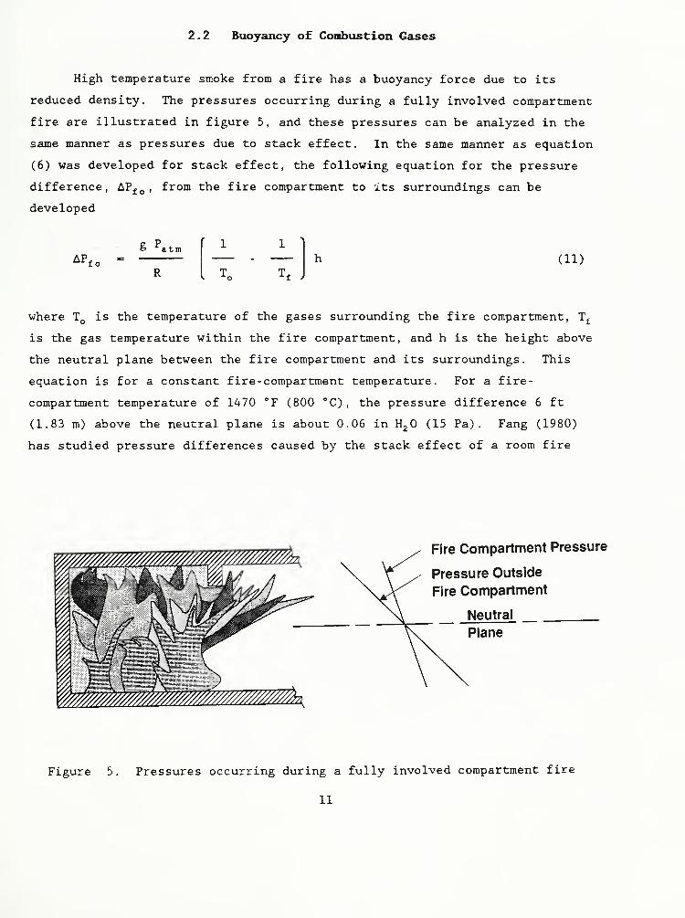
High temperature smoke from a fire has a buoyancy force due to its
reduced density. The pressures occurring during a fully involved compartment
fire are illustrated in figure 5, and these pressures can be analyzed in the
same manner as pressures due to stack effect. In the same manner as equation
(6) was developed for stack effect, the following equation for the pressure
difference,,from the fire compartment to xts surroundings can be
developed
APf O
g Pat.
R
r 1
T,
1 '
Tf -
h ( 11 )
where is the temperature of the gases surrounding the fire compartment,
is the gas temperature within the fire compartment, and h is the height above
the neutral plane between the fire compartment and its surroundings. This
equation is for a constant fire - compartment temperature. For a fire-
compartment temperature of 1470 °F (800 °C), the pressure difference 6 ft
(1.83 m) above the neutral plane is about 0.06 in H2O (15 Pa). Fang (1980)
has studied pressure differences caused by the stack effect of a room fire
Figure 5. Pressures occurring during a fully involved compartment fire
11
during a series of full scale fire tests. During these tests, the maximuin
pressure difference reached was 0.064 in H2O (16 Pa) across the burn room wall
at the ceiling.
Observation of table 1 can provide insight on conditions for which
buoyancy as opposed to stack effect is likely to be the dominate driving
force. Without broken windows, the buoyancy will dominate for large values of
at almost any location from the neutral plane. For low values of
locations far from the neutral plane, stack effect can dominate
even when windows are unbroken. When windows are broken, stack effect is even
more likely to dominate. Of course, stack effect can only be the dominate
driving force during times of significant inside- to-outside temperature
difference
.
Much larger pressure differences are possible for tall fire compartments
where the distance, h, from the neutral plane can be larger. If the fire
compartment temperature is 1290 °F (700 °C), the pressure difference 35 ft
(10.7 m) above the neutral plane is 0.35 in H2O (88 Pa). This represents an
extremely large fire, and the example is included to illustrate the extent to
which equation (11) can be applied.
2.3 Expansion of Combustion Gases
In addition to buoyancy, the energy released by a fire can cause smoke
movement due to expansion. In a fire compartment with only one opening to the
building, air will flow into the fire compartment and hot smoke will flow out
of the compartment. Neglecting the added mass of the fuel which is small
compared to the airflow and considering the thermal properties of smoke to be
the same as those of air, the ratio of the volumetric flows can be simply
expressed as a ratio of absolute temperatures.
Qo u t
Q.n
out( 12 )
where
;
12
Qout volumetric flow rate of smoke out of the fire compartment
•= volumetric flow rate of air into the fire compartment
Tput absolute temperature of smoke leaving the fire compartment
= absolute temperature of air entering the fire compartment
For a smoke temperature of 1110 "F (600 ’’C), the gas will expand to
about three times its original volume. For a fire compartment with open doors
or windows, the pressure difference across these openings due to expansion is
negligible because of the large flow areas involved. However, for a tightly
constructed fire compartment without open doors or windows, the pressure
differences due to expansion may be important.
2.4 Wind Effect
Wind can have an effect on smoke movement. The pressure,,that wind
exerts on a surface can be expressed as
1
C pwp. (13)w2
where is a dimensionless pressure coefficient, p^ is the outside air
density, and U is the wind velocity. Generally, the pressure coefficient,,
is in the range of -0.8 to 0.8, with positive values for windward walls and
negative values for leeward walls. The pressure coefficient depends on
building geometry and local wind obstructions, and the pressure coefficient
varies locally over the wall surface. Values of pressure coefficient,,
averaged over the wall area are listed in table 2 for rectangular buildings
which are free of local obstructions.
The pressure difference from one side of a building to another due to
wind effect can be expressed as
1
P,W(14)
2
13
Table 2 . Average pressure coefficients for walls of rectangular buildings
[Adapted from MacDonald, (1975)]
Building Height Building Plan
Ratio Ratio Elevation Plan
h <1w 2
1 < — < —2 w 2
1<II7 ^ ^ h
w ~ 2 H K T0.25W
— < — <42 w ^
I
Bf
L
1<i<3w 2
c
c
-3-<X<42 w
D
— < — <62 w
1 <— < —' w 2
— < — <42 w ^
WindAngle
a A
Cw for Surface
B C D
00 +0.7 -0.2 -0.5 -0.5
90° -0.5 -0.5 +0.7 -0.2
0° +0.7 -0.25 -0.6 -0.6
900 -0.5 1o cn +0.7 0.1
00 +0.7 -0.25 -0.6 -0.6
900 -0.6 -0.6 +0.7 -0.25
00 +0.7 -0.3 -0.7 -0.7
900 -0.5 -0.5 +0.7 -0.1
00 +0.8 -0.25 -0.8 -0.8
900 -0.8 -0.8 +0.8 -0.25
00 +0.7 -0.4 -0.7 -0.7
900 -0.5 -0.5 +0.8 -0.1
Note: h= height to eaves or parapet; i’= length = the greater horizontal
dimension of a building; w= width = the lesser horizontal dimension of a buililing
14
where the subscripts 1 and 2 refer to the windward and leeward sides of the
building. Examples of wind induced pressures for wind speeds from 5 to 50 mph
(2.24 to 22.4 m/s) are provided in table 1. Obviously, wind effects are most
sever at high wind speeds and when windows are broken.
In general, wind velocity, U, increases with elevation, z, above the
ground, as is expressed by the power law equation.
(15)
where is the velocity at elevation,and n is the wind exponent. Wind
data is recorded by airports and the weather service at heights, z^,of about
33 ft (10 m) above the ground. This relationship has been extensively used
to describe the velocity profile of the wind near the surface of the earth.
It assumes that there are no large obstructions near the building that could
produce local wind conditions. For buildings with such obstructions,
specialized wind tunnel studies are needed to determine the pressure loadings
due to the wind.
A value of 0.16 for the wind exponent is appropriate for flat terrain.
The wind exponent increases with rougher terrain, and for very rough terrain,
such as urban areas, a value of 0.40 is appropriate. In urban areas with a
rather constant roof level, the wind gradient can be expressed as
U (15a)
Where y is the average roof height. Wind velocity profiles are illustrated in
figure 6 for flat and very rough terrain. For further information about wind
exponents and flow coefficients the reader is referred to texts on wind
engineering such as those by Houghton and Carruthers (1976), Kolousek et al.
(1984), MacDonald (1975), Sachs (1978), and Simiu and Scanlan (1986).
15
Flat Terrain Such as a Lake Very Rough Terrain Such as a City
Figure 6. Wind velocity profiles for flat and very rough terrain
2.5 Ventilation Systems
Heating, ventilating and air conditioning (HVAC) systems frequently
transport smoke during building fires. When a fire starts in an unoccupied
portion of a building, the HVAC system can transport smoke to a space where
people can smell the smoke and be alerted to the fire. Upon detection of fire
or smoke, the HVAC system should be designed so that either the fans are shut-
down or the system goes into a special smoke control mode of operation. The
advantages and disadvantages of these approaches are complex, and no simple
consensus has been reached regarding a preferred method for various building
types. However, if neither fan shut-down nor smoke control is achieved, the
HVAC system will transport smoke to every area the system serves. As the fire
progresses, smoke in these spaces will endanger life, damage property and
inhibit fire fighting. Although shutting down the HVAC system prevents it
from supplying oxygen to the fire, system shut-down does not prevent smoke
movement through the supply and return ducts, air shafts, and other building
16
openings due to stack effect, buoyancy, or wind. Computer simulation of smoke
movement through HVAC systems are discussed by Klote (1987) and by Klote and
Cooper (1988)
.
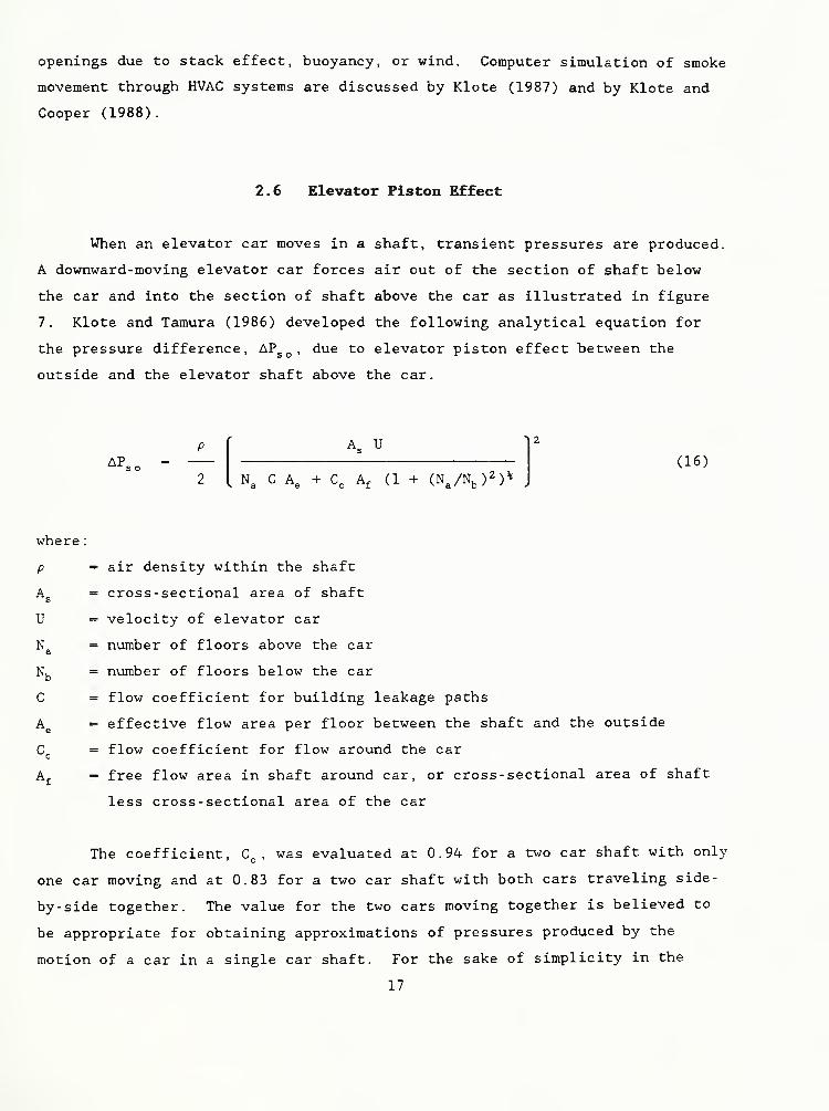
2.6 Elevator Piston Effect
When an elevator car moves in a shaft, transient pressures are produced.
A downward-moving elevator car forces air out of the section of shaft below
the car and into the section of shaft above the car as illustrated in figure
7. Klote and Tamura (1986) developed the following analytical equation for
the pressure difference, AP^^, due to elevator piston effect between the
outside and the elevator shaft above the car.
AP.
A. U
L N, C A, + C, A^ (1 + (N,/N^)2)^( 16 )
where
:
As
U
Na
Nb
C
Ae
Cc
Af
= air density within the shaft
= cross-sectional area of shaft
= velocity of elevator car
= number of floors above the car
= number of floors below the car
= flow coefficient for building leakage paths
= effective flow area per floor between the shaft and the outside
= flow coefficient for flow around the car
= free flow area in shaft around car, or cross-sectional area of shaft
less cross-sectional area of the car
The coefficient,,was evaluated at 0.94 for a two car shaft with only
one car moving and at 0.83 for a two car shaft with both cars traveling side-
by-side together. The value for the two cars moving together is believed to
be appropriate for obtaining approximations of pressures produced by the
motion of a car in a single car shaft. For the sake of simplicity in the
17
Machine Room
Figure 7. Airflow due to downward movement of elevator car
18
analysis leading to equation (16), buoyancy, wind, stack effect, and effects
of the heating and ventilating system were omitted. Omitting stack effect is
equivalent to stipulating that the building air temperature and the outside
air temperature are equal.
For the system of three series flow paths from the shaft to the outside
illustrated in Fig. 1, the effective flow area,,per floor is
A1
A 2(17)
where is the leakage area between the lobby and the shaft, A^ is the
leakage area between the building and the lobby, and A^^^
is the leakage area
between the outside and the building. In a similar manner to the development
for stack effect, the pressure difference, can be expressed as
APii = AP,^ (A,/A,,)2 (18)
This series flow path analysis does not include the effects of other
shafts such as stairwells and dumbwaiters. Provided that the leakage of these
other shafts is relatively small compared to A^^ ,
equation (17) is appropriate
for evaluation of A^ for buildings with open floor plans. Further, equation
(18) is appropriate for closed floor plans, provided all the flow paths are in
series and there is negligible vertical flow in the building outside the
elevator shaft. The complicated flow path systems probably require case by
case evaluation which can be done by using the effective area techniques
presented in the ASHRAE smoke control manual (Klote and Fothergill 1983).
To test the above theory, experiments were conducted in a hotel in
Toronto, Ontario, Canada. Figure 8 shows measured pressure differences across
the top floor elevator lobby while a car was descending. Also shown is the
calculated pressure difference which is in good agreement with the
measurements. This experiment is described in detail by Klote and Tamura
(1986). The pressure difference, APj^^,can not exceed the upper limit of
19
Figure 8. Pressure difference, APj^^ , across elevator lobby
of a Toronto hotel due to piston effect
As A, u
Af A,, ,
(19)
where the subscript u denotes the upper limit. This relation is for unvented
elevator shafts, or for which the vents are closed. The pressure difference,
(AP^^), is strongly dependant upon U, and . For example, figure 9 shows
the calculated relationship between (APj^^)^ and U due to one car moving in a
single car shaft, a double car shaft and a quadruple car shaft. As expected
the (AP^^)^ is much greater for the single car shaft. It follows that the
potential for smoke problems due to piston effect in single car shafts is much
greater than in multiple car shafts. Comparison of stack effect induced
20
Car Velocity (fpm)
Figure 9. Calculated upper limit of the pressure difference,from the elevator lobby to the building due to piston effect
pressure differences indicates that they can be larger than those of other
driving forces (table 1).
Operation of elevators by the fire service during a fire can result in
smoke being pulled into the elevator shaft by piston effect. It seems a safe
recommendation that fire fighters should favor the use of elevators in
multiple car shafts over ones in single car shafts. Klote (1988a) developed
another analysis of piston effect including the influence of elevator smoke
control, and experiments conducted by Klote and Taraura (1987) were in good
agreement with this theory.
21
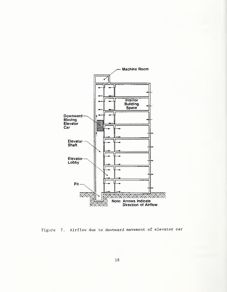
3. LOCATION OF NEUTRAL PLANE
In this section methods of determining the location of the neutral plane
are described for a single shaft connected to the outside only. The methods
of effective area can be used to extend this analysis to buildings. Using
these neutral plane locations, the flow rates and pressures throughout the
building can be evaluated to the extent that the series flow model of section
2.1 is applicable.
3 . 1 Shaft with a Continuous Opening
The flow and pressures of normal stack effect for a single shaft
connected to the outside by a continuous opening of constant width from the
top to the bottom of the shaft is illustrated in figure 10. The following
Continuous Opening of
Figure 10. Normal stack effect between a single shaft
connected to the outside by a continuous opening
22
analysis of this flow and the resulting location of the neutral plane was
developed by McGuire and Tamura (1975). The pressure difference from the
shaft to the outside is expressed by equation (6). The mass flow rate, dm^^^ ,
through the a differential section, dh, of the shaft below the neutral plane
is
C A'J 2 AP,, dh C A'J 2 b h dh ( 20 )
where
6 t m 1 1
and where A' is the area of the opening per unit height. To obtain the mass
flow rate into the shaft, this equation can be integrated from the neutral
plane (h = 0) to the bottom of the shaft (h = - )
.
m. C A' J 2 b ( 21 )
In a similar manner an expression for the mass flow rate from the shaft
can be developed, where H is the total height of the shaft.
mout C A' (H - )^^^ I 2 . b ( 22 )
For steady flow, the mass flow rate into the shaft equals that leaving
it. Equating equations (21) and (22), cancelling like terms, rearranging, and
substituting equation (5) yields
^ 1
H 1 + (T3/TJI /3
( 23 )
23
For an inside temperature of 72 “F (22 °C) and an outside temperature of
0 °F (-18 °C), the neutral plane is located 48.8 percent up the height of the
shaft which is slightly different from the generally accepted approximation of
halfway up the shaft.
3.2 Shaft With Two Vents
Normal stack effect for a shaft with two openings is illustrated in
figure 11. The pressure difference from the shaft to the outside is expressed
by equation (6). To simplify analysis, the distance, H. between the openings
is considered much greater than the height of either opening. Thus the
Figure 11. Stack effect for a shaft with two openings
24
variation of pressure with height for the openings can be neglected, and the
mass flow rate into the shaft can be expressed as
m, C (24)
and the mass flow rate out of the shaft is
mout C A, J 2 p, b (H - ) (25)
Where and A^^ are the areas above and below the neutral plane. Equating
these two flows as was done above yields
^ _1
H 1 + (T,/T„)(A^/AJ2(26)
For an inside temperature of 72 °F (22 °C)
,
an outside temperature of 0
°F (-18 °C), and equal areas (A^^ = A^ ) ,the neutral plane is located 46.4
percent up the height of the shaft which is only a little less than the case
of the continuous opening (48.8 percent). The location of the neutral plane
is highly dependant on the ratio A-^/A^. For A^/A^ that approaches zero,
approaches H. This means that if the area at the bottom is very small
compared to the area at the top, then the neutral plane is at or near the top
area. Equation (26) is a strong function of the flow areas and a weak
function of temperature
.
25
Continuous Opening of
Constant Width
Figure 12. Normal stack effect between a single shaft connectedto the outside by a vent and a continuous opening
3 . 3 Vented Shaft
The flow and pressures of normal stack effect for a shaft connected to
the outside by a vent and a continuous opening are shown in figure 12. The
following analysis is for a vent above the neutral plane, but a similar one
can be made for a vent below the neutral plane. This analysis is an extension
of one by McGuire and Tamura (1975) for a top vented shaft. The mass flow into
the shaft is expressed by equation (21). For simplicity of analysis, the
height of the vent is considered small in comparison to the shaft height, H.
Thus, a constant pressure difference can be used to describe the flow through
26
the vent. The mass flow out of the shaft is the sum of the flow out of the
continuous opening, expressed as equation (22), plus the flow out of the vent
of area located at an elevation of above the shaft bottom.
°>out= C A' (H - J 2 b + C A^ J 2 b (H^ - H„) (27)
3
Continuity of mass equation for the shaft can be written as
— C A' (H - H^)3/2 J 2 p^ b + C A^ J 2 p, b (H, - H^) =
3
(28)
C A’ J 2 b3
Cancelling like terms and incorporating equation (5) results in
2 2— A' (H - (h^ . h^)1/2 = A' H^3/2 (29)3 3
As would be expected, this equation reduces to equation (23) for A^ = 0
.
Equation (29) can be rearranged as
2 A' H (H - (Hv - 2 A' H+ - = 0 (30)
3 A^ H H 3 A^ H ^ ^
For relatively large vents, the ratio A'H/A^ approaches zero. As A'H/A^
approaches zero, the first and third terms in the above equation approach
zero, and the equation is reduced to Thus the neutral plane is at or
near the vent elevation, for a vent area very much greater than the area of
the continuous opening (A'H)
.
As with equation (26), the above equation is a
strong function of the flow areas and a weak function of temperature.
27
Regardless of whether the vent is above or below the neutral plane, the
neutral plane will be located between the height described by equation (23)
for an unvented shaft and the vent elevation, . Further, the smaller the
value of A'H/Ay, the closer the neutral plane will be to .
4. FRICTION LOSS IN SHAFTS
In the discussions above, the pressure losses due to friction in shafts
were assumed negligible. If the flow rate in a shaft is relatively small,
this assumption is appropriate. However, for high flow rates in shafts,
friction losses can be significant. For straight shafts such as elevator
shafts, the friction loss, AP^ , is expressed by the Darcy equation
L U2
AP, = f p (31)
De 2
where f is the friction factor, L is the length of the duct, is the
effective diameter of the duct, p is the density of the gas in the duct, and U
is the average velocity in the duct. Incorporation of the effective diameter
allows evaluation of ducts with various geometries, and the reader is referred
to the ASHRAE Handbook (1985) for a discussion of effective diameters. The
friction factor is a function of the Reynolds number and the relative
roughness of the duct, and it can be obtained from the well known friction
factor diagrams reproduced in most elementary fluid dynamics texts. For
calculations of losses in shafts, the flow is approximated as a function of
mass flow rate, m, in the shaft by Klote and Fothergill (1983) as
APf = (m/Cj2 (32)
where
28
c
2 p a2
f L
for straight shafts with cross sectional area of A, and L is one floor height
of the shaft. For stairwells the friction factor is nearly constant over the
relevant range of flows, and is approximated by a constant. is
dependant on the cross sectional area, A, of the stairwell, and can be
expressed as 'A based on research of Tamura and Shaw (1976) . An
average value of ' = 49 (.25) is recommended for area in ft^ (m^ ) ,pressure
loss in inches H2O (Pa) per floor, and mass flow rate in Ib/min (kg/s). Based
on the example analyses presented later in this paper, the flows due to stack
effect in stairwells are on the order of;
Ib/min (kg/s)
60 (0.5) with all doors closed and no vents, and
600 (4.6) with a top vent and an exterior door open.
For a stairwell with a cross sectional area of 120 ft^ (11 m^ )
,
these flows
result in the following pressure losses per floor:
in H2O (Pa)
0.0001 (0.025) with all doors closed and no vents,
0.01 (2.5) with a top vent and an exterior door open.
These losses can be compared to the pressure difference due to stack effect as
expressed by equation (6). For an outside temperature of 0 °F (-18 '’C),and
an inside temperature of 72 °F (22 “C)
,
the pressure due to stack effect is
about 0.02 in H2O (5 Pa) at one floor [10 ft (3 m)
]above the neutral plane.
A height of one floor was used so that the basis of comparison would be the
same with the friction losses. These calculations indicate that pressure
losses due to friction are generally negligible for shafts with all doors
closed and no vents, but shaft friction can be significant for many common
situations such as shafts with open doors or vents.
29
5. STEADY SMOKE CONCENTRATIONS
Tamura (1969) developed a simple method to calculate steady smoke
concentrations, and this steady smoke approach is addressed here because it
leads to an understanding of smoke flow under limited conditions. This model
is based on the assumption of perfect mixing. That is, that the smoke
concentration is uniform throughout a space, and consequently that mixing of
flows into the space occurs instantly. This assumption is appropriate to the
extent that the air in the room is well mixed due to the effect of a
ventilation system, motion of people, room air currents due to convective heat
transfer, cooling fans in electronic equipment, or other effects. Zone models
addressed later do not have this limiting assumption.
The mass flow rate of a substance into a space equals the mass flow rate
of that substance out of the space. For a building space i, this mass balance
relation can be expressed as
2j
(m1 j ).n 2 (n'ji Ci)out (33)
where c^ and c^ are the concentrations in spaces i and j respectively, and the
subscripts in and out indicate flow into and out of space i respectively.
This equation can be solved for the smoke concentration of space i
= 2j
)in / 2J
out (34)
For a number of informative cases, the pressures and mass flow rates can
be calculated as discussed above, and equation (34) can be used to determine
the steady smoke concentrations Such calculations of mass flow rate are time
consuming and limited to a few simple cases of building leakage conditions.
However, the computer models to calculate air these flows are addressed in the
next section.
30
6 . NETWORK MODELS
The above methods for determination of neutral plane are limited to a
few simple geometries. A number of network computer models have been
developed that can be used to analyze flows and pressures in buildings with
very complicated flow systems. It should be noted that these network models
differ from zone models which are discussed later. This section provides an
overview of these programs. Because of the number of programs involved, an
exhaustive cataloging of network models is beyond the scope of this paper.
However, Feustel and Kendon (1985) at Lawrence Berkeley Laboratory have
prepared a literature review of network models used for air flow analysis in
buildings, and Said (1988) of the National Research Council of Canada has
evaluated several such models with respect to applicability for smoke control
analysis
.
Some computer programs only simulate airflow in buildings such as the
ventilation models of Sander and Tamura (1973) and Sander (1974) and the smoke
control model by Klote (1982). Other programs model smoke movement within a
building such as ones by Butcher, et al . (1969), Barrett and Locklin (1969),
Wakamatsu (1977), Evers and Waterhouse (1978), and Yoshida et al.
(1979).
Some programs include extensive heat transfer algorithms such as the Thermal
Analysis Research Program (TARP) by Walton (1984).
31
6 . 1 Network Model Concept
In all the above computer programs, a building is represented by a
network of spaces or nodes, each at a specific pressure and temperature.
Vertical shafts such as stairwell, elevator shafts, mail chutes, dumbwaiters,
mechanical shafts, and electrical shafts are modeled by a series of vertical
spaces, one for each floor. Air flows through openings from regions of high
pressure to regions of low pressure. These flow paths may be open windows or
doors,gaps around interior doors
,or very narrow cracks around
weathers tripped windows and doors. Less obvious but no less important leakage
paths are construction cracks, such as where walls meet floors, where ceiling
tiles meet a steel suspension grid, where walls interface with window frames
and door frames, around electrical fixtures and outlets, and at plumbing
fixtures. Air flow through these paths is a function of the pressure
difference across the path and the path geometry. Outside pressures
incorporate the effects of air temperature and wind. The building's heating,
ventilating and air conditioning (HVAC) systems are also taken into account.
In the smoke movement models, smoke generated in the fire compartment
flows through openings to adjacent spaces and is carried along with building
air currents through complex paths to locations remote from the fire. In some
of the models, the temperature of spaces increases due to the flow of hot
smoke, while heat is transferred from the smoke to the building's interior
surfaces
.
Each network model is to some extent unique, depending on its intended
application. However, the computer programs are similar in many respects, and
the equations provided in the following sections form a general description of
this class of model.
6 . 2 Mass Flow Rates
For the same conditions of pressure and temperature, there are
negligible differences in fluid properties between clean air and smoke.
32
Consequently, the network smoke movement models calculate only air flows, and
as the need arises, smoke concentrations in air are evaluated. Accordingly,
the air movement portion of the program can be described by the same equations
that describe air movement for ventilation or energy analysis programs.
The mass flow rate,,to space i from space j through a flow path
with cross-sectional area is expressed by the flow equation
(35)
where and are the pressures of spaces i and j, respectively, S is the
sign of (Pj - Pi ) ,and C is the flow coefficient. Generally, space j is
another location within the building, however, it can be outside the building.
An outside pressure Pj is dependent on outside air temperature and wind
effects. Considerable data concerning building air leakage is provided in the
ASHRAE Handbook of Fundamentals (1985, Chapter 22). Typical leakage areas of
construction cracks in walls and floors of commercial buildings have been
tabulated by Klote and Fothergill (1983, Appendix C) . Strictly speaking,
network models have the limitation that flow between two spaces can only be in
one direction. However, some of these models allow bidirectional flow in the
vicinity of the fire. For a building space i, the mass balance equation is
(36)0j
In general, the mass flows are described by equation (35), however, the
effects of ventilation systems can be expressed by incorporating a constant
flow term from a ventilation space j
.
By substitution of equation (35) into equation (36) and expressing in
terms of space pressure, a system of equations can be obtained for all n
spaces of a building network.
33
( 37 )
“l (Pi. Pa. . Pn) “
(Pi. Pa. . ... Pi. .
(Pi. Pa. . Pn) -
Thus the building; pressures, to , are solved simultaneously by
solving n number of mass balance equations. In reality, the number of
pressures included in an equation m^ -= 0 are only P^ and those pressures of
spaces directly connected to space i. Because each of the equations is
nonlinear as represented by equation (35), it is generally difficult to solve
these systems of equations in an analytical way. A discussion of the
numerical techniques involved is beyond the scope of this paper. However,
this problem is mathematically similar to the analysis of water flow in piping
networks the computer solution of which the civil engineering community has
had considerable success. Wood and Rayes (1981) have evaluated several
commonly used algorithms for the water flow networks
.
6.3 Unsteady Smoke Concentrations
As with the method for calculating steady smoke concentrations,
simulation of unsteady smoke flow in network models is based on the perfect
mixing assumption. At an arbitrary time, t = k At (k = 0 , 1 , 2 , ...) where At
is a time interval, the balance of concentrations for space i is
Cj)in (""ji Ci)„, jAt = V.p.Ac, (38)
where is the air volume of space i, c^ and Cj are concentrations in spaces
i and j, respectively, and Ac^ is the change of concentration within space i
during the time interval. The change in concentration can be expressed as Ac^
= c^ (k+1) - c^ (k),where k refers to time steps. From equation (36) the
following equation for the concentration in space i was derived by Wakamatsu
(1977)
34
SMc.I'
SM^ AtCi(k+1) - + (c. (k) - SMc^/SM. )exp (39)
Pi
where
SMc, = 2 [m,,(k) Cj(k)],„j
and
Thus the concentrations, c,,at time step k+1 can be calculated in terms
of the concentrations and mass flow rates at time step k. The concentration
in the fire compartment is the driving force, and many models like Wakamatsu
(1977) and Evers and Waterhouse (1978) assume that the fire compartment
concentration is constant throughout the fire. The whole fire space is
assumed at a uniform temperature. This can be thought of as modelling smoke
movement due to smoldering fire or, neglecting early fire growth, smoke
movement due to an intense fire that exists when a compartment is fully
involved in fire. The model by Yoshida et al. (1979) accepts a user defined
time profile of smoke concentration and temperature of the fire compartment.
A significant shortcoming of the network smoke movement models is their
treatment of the fire compartment and spaces directly connected to it. In
these spaces smoke generally is not perfectly mixed, but forms a hot upper
layer. Whenever, a gas flows into a compartment in which the gas has some
buoyant force, there is a tendency toward forming an upper layer. The extent
to which the forces promoting mixing (ventilation systems, convection
currents, etc.) interfere with smoke stratification is unknown. Research is
needed to develop an understanding of smoke movement far from the fire source.
Network models should be used with caution concerning their particular
assumptions and the limitations of knowledge in this entire area.
35
6.4 Unsteady Temperat\ires
Network models for building energy analysis, such as TARP (Walton 1983)
simulate heat transfer in considerable detail including solar gains though
windows, walls and roof, as well as, heat transferred between interior
building components by conduction, convection and radiation. It should be
noted that the energy models calculate flows and temperatures at one to three
hour intervals which is inappropriate for simulation of building fires.
Wakamatsu handles convective heat transfer, and calculates unsteady
temperatures for building spaces. However, most of the ventilation models
such as Sander and Tamura (1973) and some of the smoke movement models such as
Evers and Waterhouse (1978) and Yoshida et al . (1979) assume constant, user
defined temperatures throughout the building. This can be appropriate for
ventilation models applied to buildings that have heating and cooling systems
to maintain nearly constant temperatures. It is probably appropriate for
simulation of smoke movement due to a smoldering fire. While the constant
temperature assumption is unrealistic with respect to flaming fires, it still
can be used to gain some insight into gross smoke movement in large buildings.
7 . ZONE MODELS
The common feature of zone fire models is that they describe the bulk of
a room's fire-generated environment, away from fire plumes and near-surface
boundary flows, as being divided into two uniform-property zones: an upper
layer of 'hot' air, heavily contaminated with the fire's products of
combustion, i.e., the smoke, and a lower layer of relatively uncontaminated
and relatively cool air. Examples of zone models are those by Zukoski and
Kubota (1980), Hitler and Emmons (1981), Quintiere, et al. (1981), Cooper
(1982), Tanaka (1983), and Jones (1985). A comparison of the various models
is beyond the scope of this paper. However, the mathematical framework of
each of these models has much in common with the others as is obvious from the
review of zone models by Jones (1983). Further, Hitler (1985) compares the
features of three of these fire models.
36
The intent of this section is to provide a simple description of zone
models in order show the potential of these models in addressing smoke
movement in buildings due to stack effect. It should be realized that each
model has its own level of detail and its own unique assumptions in describing
mathematically the processes of combustion, heat and mass transfer, and flow
dynamics. The following, adopted from Klote and Cooper (1988), is a brief
generic description of compartment fire phenomena and of the class of zone-
t3rpe compartment fire models of these phenomena. For more extensive
discussions of the overall phenomena the reader is referred to Cooper (1984)
and Kennedy and Cooper (1987) for qualitative aspects and to the above-
referenced model references for quantitative aspects.
7 . 1 Compartment Fire Phenomena
Refer to Figure 13. In a room of fire involvement, air which supports
the combustion process is entrained into the combustion zone and mixes with
combustion products. There the mixture of gases and fire-generated
particulates are heated and driven upward. These materials form a buoyant
plume which continues to entrain and mix with air and cool as it rises above
the combustion zone to the ceiling. A portion of the energy released from the
combustion zone is transferred by radiation to the walls, floor and ceiling.
Figure 13. Stratified smoke flow as simulated by zone fire models
37
As a result of this, the temperature of these materials begin to increase.
As the plume impinges on the ceiling it is redirected outward as a
relatively high temperature radial ceiling jet which heats by convection the
ceiling surface. Having reached the bounding walls of the room, the buoyant
plume gases and particulates eventually redistribute themselves across the
entire upper portion of the room and begin to form a relatively quiescent,
elevated- temperature smoke layer. As the plume continues to entrain air from
the lower portion of the room and to add new material to upper portion of the
room the smoke layer grows in thickness and changes in composition.
The interface which separates the upper smoke layer from the lower air
layer typically drops eventually below the tops of doors, windows, or other
open vents. The smoke then flows out of the fire room and into adjacent rooms
or into the atmosphere. At a given vent this outward flow is often exchanged
and mixed with inward flowing fresh air. These multi-directional vent flows
are driven by room- to-room, cross-vent, hydrostatic pressure differences which
vary as a function of elevation and which can change sign one or more times
across the vertical extent of a vent.
High temperature smoke which enters an adjacent space is relatively
buoyant there and rises to the ceiling by buoyant flow processes which are
reminiscent of those discussed above for the fire plume. For example, as
illustrated in Figure 13, upper layer gases flowing through a doorway can form
an upward flowing door jet, which can begin to form and then add to the growth
of an upper layer in an adjacent room. Thus, smoke -filling and -transport is
initiated in the adjacent spaces of the facility and beyond.
As mentioned, the major assumption of zone models is that they simulate
the fire - generated environment in each room as being divided into an upper,
elevated- temperature smoke layer and a lower, relatively- cool,and less-
contaminated air layer. This is illustrated in Figure 13.
For simplification, the temperature and composition of each layer is
considered homogeneous. In the bulk of the room, away from plumes, vent-
38
flows, and near- surface boundary flows, the environment is relatively
quiescent and the pressure, P, is estimated by hydrostatics, i.e., P - Jgpdz,
where g is the acceleration of gravity, p is the density, and z is elevation.
A Bernoulli-equation formulation of the momentum equation and z-dependent,
cross-vent, pressure differences are used to compute the z-dependent velocity
of room-to-room mass exchanges. Rules for depositing the vent flows into the
upper or lower layer of the receiving room are established.
The upper and lower layer of each room is required to satisfy
conservation of mass, energy, and species and the equation of state. This
leads to a set of time -dependent differential equations in the independent
variables. These are the variables which can be used to describe completely
the state of both layers, i.e., the overall fire environment, in the room.
The equations for all rooms of a simulation taken together form the complete
equation set for the model.
The following equations, taken from the CCFM zone model formulation of
Cooper and Forney (1987), is an example of a fully-general set of equations
for an arbitrary room of a simulation. They are given in the independent
variables p, pressure at the floor of the room; Vy,volume of the upper layer;
Py and py ,densities of the upper and lower layer; and c^ y and c^ y,
concentration of product of combustion i in the upper and lower layer. The
equations for the dependent variables, Ty and Ty,the temperatures of the
upper and lower layers, are also shown. As can be seen below, these are
obtained directly from the equation of state of a perfect gas, which is
assumed traditionally to be a useful approximation in zone fire model
formulations. The complete set of equations is valid when the layer interface
is between the floor and the ceiling of the room, i.e., whenever 0 < Vy < V,
the volume of the room.
pressure at the floor of the room:
dP/dt = [(7 - 1)/V](qy + qy)
39
volume of the upper layer:
dV^/dt - [(7 - 1)/(7P)][(1 - Vu/V)qu - (VuA)qL]
densities of the upper and lower layer:
dpu/dt - (1/V„)(mu - PudVy/dt)
(AO)
dp^/dt = [1/(V - Vu)](mL + p^dV^/dt)
concentration of product of combustion i in the upper and lower layer:
“[ ^/(Pu^U ^ ] (^i , U
’
dc,_L/dt = (1/[Pl(V - V„)])(M,_l l)
absolute temperature of the upper and lower layer:
Tu = P/(PuR); Tl = P/(PlR)
Beside the independent variables and the physical constants 7 ,ratio of
specific heats, and R, the gas constant, the right-hand- side of the above
equations depend only on: q^ and q^ ,the net rate of enthalpy plus heat
transfer plus energy release flowing to the upper and lower layer; m^ and m^
,
the net rate of mass flowing to the upper and lower layer; and ^ and M.
the net rate of product i flowing to the upper and lower layer. At any
instant of time during the course of a fire simulation, the contributions to
these terms are dependent on the details of the individual algorithms which
describe mathematically the combustion and the various mass and heat transfer
processes, e.g., the plume equations, rules for distributing vent flows into
the two layers of the receiving room, and the equations for radiative
exchanges
.
In principle, the above equation set should contain the equation set of
any zone -fire model. However, the type and sophistication of the solution
40
techniques that could be used, whether analytic or, more t3TJically, numeric
are not unique. Also, the actual form of (the right hand side of) these
equations would depend on the particular details of the collection of
algorithms which describe the individual physical phenomena. The CCFM will be
relatively flexible with regard to choice of these details. It is being
developed in a manner that will allow for a wide range of modeling detail,
from basic to "benchmark" simulations.
7.2 Application to Higih Rise Buildings
Tanaka (1983) used a zone model to simulate smoke transport in large
buildings, and figures 14 through 17 show his analysis of smoke conditions in
a ten story building with two shafts at 0.5, 1.0, 3.0 and 4.5 minutes after
ignition. Even though Tanaka's analysis did not include naturally occurring
stack effect nor wind effect, this work is discussed here to show the
capabilities of zone modelling with respect to large buildings. The
dimensions of the rooms, shafts, interior openings and exterior openings for
these analyses are listed in table 3. At 0 . 5 minutes (figure 14), both shafts
for the most part have filled with smoke, and smoke is flowing out of the
shafts on most floors. It should be noted that for most of the interior
openings, the flow is bidirectional, and at some locations the flow is
tridirectional . At 1.0 and 3.0 minutes (figures 15 and 16), the smoke spread
and the temperatures of the upper layers have increased.
Table 3. Dimensions used for Tanaka's (1983) zone modelsimulation of smoke movement in a ten story building
Item Dimensions
all rooms1st shaft2nd shaft
13 X 20 X 9.8 ft high (4 x 6 x 3 m high)13 X 20 X i39 ft high (4 x 6 x 42.5 m high)
13 X 20 X 126 ft high (4 x 6 x 38.5 m high)
exterior openingon 1st floor 3.3 X 3.3 ft (1 X 1 m).
exterior openingson other floors 0.33 X 3.3 ft high (0.1 x 1 m high)
3.3 X 6.6 ft high (1 x 2 m high)interior openings
41
Note: Number under a ceiling with no arrow indicates temperaturerise above ambient (°C), and number at an opening with an arrowindicates flow rate (kg/s). (A temperature rise of 1 °C = a riseof 1.8 "F, and 1 kg/s = 132 Ib/min.)
Figure 14. Smoke flow at 0.5 minutes after ignition in a tenstory building calculated by a zone model
[Adapted from Tanaka (1983)]
42
Note: Number under a ceiling with no arrow indicates temperature
rise above ambient (°C), and number at an opening with an arrow
indicates flow rate (kg/s). (A temperature rise of 1 C = a rise
of 1.8 °F, and 1 kg/s = 132 Ib/min.)
Figure 15. Smoke flow at 1 . 0 minutes after ignition in a ten
story building calculated by a zone model
[Adapted from Tanaka (1983)]
43
Note; Number under a ceiling with no arrow indicates temperaturerise above ambient (°C), and number at an opening with an arrowindicates flow rate (kg/s). (A temperature rise of 1 °C = a riseof 1.8 °F, and 1 kg/s = 132 Ib/min.)
Figure 16. Smoke flow at 3.0 minutes after ignition in a ten
story building calculated by a zone model[Adapted from Tanaka (1983)]
44
Note: Number under a ceiling with no arrow indicates temperaturerise above ambient (‘’C), and number at an opening with an arrowindicates flow rate (kg/s)
.(A temperature rise of 1 “C = a rise
of 1.8 ”F, and 1 kg/s = 132 Ib/min.)
Figure 17. Smoke flow at 4.5 minutes after ignition in a tenstory building calculated by a zone model
[Adapted from Tanaka (1983)]
45
The current zone models assume instant plume rise and instant lateral
smoke transport within a compartment. This omission can give rise to
unrealistically quick smoke propagation in large buildings. Data from full-
scale building and scale model experiments are needed to evaluate these
effects fully.
At 4.5 minutes (figure 17), a fire induced stack effect has been
achieved with flow from the outside into the building on the lower five floors
and with flow out of the building on the upper five floors. Of course, this
stack effect is due to the elevated temperatures inside most of the building.
It is interesting that the flow on the bottom floor, on upper two floors, and
through all exterior opening is unidirectional. In this example, the smoke
spread was extensive even though both shafts were top vented. However, the
vent areas for this calculation were 1.1 ft^ (.1 m^ ) which is small for shaft
vent opening. Network calculations discussed in the next section also show
extensive smoke spread through buildings with vented shafts under conditions
of normal stack effect.
It can also be seen from figure 17 that at 4.5 minutes the upper layer
in most of the rooms has descended to or very near to the floor. Thus these
rooms can be thought of as being almost entirely at the upper layer
conditions. So for this example, the zone model predicts room conditions that
almost match the prefect mixing assumption of the zone models. The treatment
of shafts by these two models is very different. Zone models treat shafts as
another room with upper and lower layers as illustrated in figures 14 through
17 . Network models treat shafts as a vertical series of perfectly mixed
spaces, one space for each floor as are illustrated in examples in the next
section. Intuitively it seems that the zone approach might be more
appropriate for straight open shafts such as elevator shafts, and that the
network approach might be more appropriate for shafts where rising flow is
accompanied by many changes in direction such as with stairwells. However,
smoke could behave differently from either approach, and research is needed in
this area.
46
8. STEADY FLOW NETWORK CALCDLATIONS
The inability to simulate multi -directional flow is a shortcoming of
network models. Where the pressure difference due to stack effect is
sufficiently large, it will dominate the fire induced pressures resulting in
unidirectional flow. Generally, the pressure difference due to buoyancy is on
the order of .1 in H2O (25 Pa), and this is usually the most important fire-
induced pressure. For tall buildings during times of extreme outside
temperature, stack effect pressure differences can be one or two orders of
magnitude greater than the buoyancy value. However, stack effect pressure
differences will still approach zero near the neutral plane. When considering
gross smoke flows throughout a building, some inaccuracies near the neutral
plane can be accepted. Thus, network models can be used to gain some
understanding of the gross smoke flow under stack effect conditions.
Table 4. Flow areas and other data about building for example analyses
Flow AreasFlow areas per floor: ft2 (m^ )
Exterior walls 0.84 (0.078)Between floors 0.40 (0.037)Stairwells to building with door closed 0.20 (0.019)Stairwells to building with a door 10.00 (0.929)
Elevator to building 1.20 (0.111)Elevator vent at top of shaft 4.00 (0.372)Stairwell vent an top of shaft 10.00 (0.929)
Other data:
Exterior air temperature 0 °F (-18 °C)
Interior air temperature (except where noted belowfor cases 4A and 6A) 72 'F (22 °C)
Fire Floor (4th floor) for cases 4A and 6A 800 °F (427 “C)
Temperature above the 3rd floor for all shaftsof case 4A 350 “F (177 °C)
Temperature above the 3rd floor for elevatorshaft and west stairwell of case 6A 350 °F (177 °C)
Flow coefficient for all flow paths .65
Height between floors 10.0 ft (3.05 m;
Location of fire fourth floor
47
150 ft (46 m)
Shown on Figures 19-24 and 28-31.
Figure 18. Floor plan of building used for example analyses
To study the effects of vents and open doors, an example building was
devised and network calculations were performed for six cases. The building
is twenty stories, each 50 by 150 ft (15 by 46 m) with an elevator shaft and
two stairwells as shown in figure 18. The height between floors is 10.0 ft
(3.05 m) . The flow areas and other data for the analysis are listed in table
4. The leakage areas were selected for a building of about average tightness.
The leakage areas of the walls and floors are based on data in appendix C of
the ASHRAE Smoke Control Manual (Klote and Fothergill 1983) . The leakage
areas of the elevator walls and doors are based on data of Tamura and Shaw
(1976). The following cases were analyzed for an outside temperature of 0 °F
(-18 "C) and an indoor temperature of 72 °F (22 °C):
1. building without any vents or open doors,
2. building with a top vented elevator shaft,
3. building with a top vented stairwell,
4. building with a top vented elevator shaft and a top
vented stairwell.
48
5. building with a top vented elevator shaft and a
stairwell with a top vent and an open exterior, first
floor door, and
6. building with a top vented elevator shaft and a
stairwell with an open exterior, first floor door.
Cases 4 and 6 were recalculated with elevated shaft temperatures as
cases 4A and 6A. The conditions of doors and vents for these cases are listed
in table 5. For all these cases, the fire was on the fourth floor. Mass flow
calculations were made with the ASCOS program (Klote and Fothergill 1983), and
the resulting mass flow rates are listed in tables 6 through 11. Steady smoke
concentrations relative to the fire floor concentration were calculated using
these mass flow rates and equation (34) ,These concentrations and directions
of mass flow are shown on figures 19 through 24. Steady smoke concentration
analysis was employed, because this provides a basic level of understanding of
some of the processes involved in this type of smoke transport. However, some
questions can only be addressed by an unsteady analysis, as is discussed
later
.
In the following discussion of these six cases, some thought should be
given as to the desired benefits of actions that could be taken to modify
smoke flow. Three possible benefits are:
• Reduction in hazard conditions on the floors of a
building
• Reduction in hazard conditions in a stairwells or an
elevator shaft
• Reduction in smoke concentration on the fire floor
However important the last benefit might be, these analyses can not
address it in that they consider the fire floor concentration constant. With
49
regard to the first two potential benefits, a hazard analysis of the smoke
concentrations is beyond the scope of this paper.
Table 5. List of vent and door conditions for example analyses
CaseElevator East Stairwell East Stairwell First
Top Vented Top Vented Floor, Exterior Door Open
1 No No2 Yes No3 No Yes4 Yes Yes5 Yes Yes6 Yes No4A Yes Yes6A Yes No
NoNoNoNoYesYesNoYes
Note: All doors not addressed in the table are closed including all doors ofthe west stairwell. Areas of openings are listed in table 3.
8.1 Building with Doors Closed and No Vents (Case 1)
Buildings with all doors closed and without any vents are not common in
the United States. However, this case was included to provide a comparison
with other cases. As expected, the neutral planes for all the shafts are at
the same elevation (figure 19). The concentrations below the fire floor are
all zero, but this is not always so as will be shown later.
It is interesting to note that for every floor above the fire floor, the
concentration decreases by about an order of magnitude up to the neutral
plane^ . This pattern is true for all six cases analyzed. The concentrations
at each level of the three shafts are the same, even though the leakage areas
to the stairwells are much smaller than those to the elevator shaft. Because
shaft friction is negligible, the pressures in all the three shafts are
de’scribed by equation (2), Pg “ S Because the temperature is the
^Concentrations less than 0.1 % of the fire floor are not shown on
figures 19 through 24.
50
West
Stairwell
Elevator
Shaft
East
Stairwell
Note: Arrows indicate direction of airflow. The magnitudes of
air flow rate are listed in table 6, and the flow areas data are
listed in table 4. Smoke concentrations are relative to the fire
floor concentration
Figure 19. Calculated smoke concentrations due to a fourth floor fire in a 20
story building without any vents or open doors (Case 1)
51
Floor
20
19
18
17
16
15
14
13
TT11
10
9
8
7
6
5
4
3
2
1
West Elevator East
Note: Arrows indicate direction of airflow. The magnitudes of
air flow rate are listed in table 7, and the flow areas data are
listed in table 4. Smoke concentrations are relative to the fire
floor concentration
Figure 20. Calculated smoke concentrations due to a fourth floor fire in a 20
story building with a top vented elevator shaft (Case 2)
52
West
Stairwell
Elevator
Shaft
Note: Arrows indicate direction of airflow. The magnitudes ofair flow rate are listed in table 8, and the flow areas data arelisted in table 4. Smoke conf entrations are relative to the firefloor concentration
Figure 21. Calculated smoke concentrations due to a fourth floor fire in a 20story building with a top vented stairwell (Case 3)
53
Floor
20
19
18
17
16
15
~T^13
12
11
10
9
8
7
6
5
4
3
2
1
WestStairwell
Elevator East
Stairwell
Note: Arrows indicate direction of airflow. The magnitudes offlow rate are listed in table 9, and the flow areas data are
listed in table 4. Smoke concentrations are relative to the firefloor concentration
Figure 22. Calculated smoke concentrations due to a fourth floor fire in a 20story building with top vents in elevator and stair shafts (Case 4)
54
West
Stftirwell
Elevator
Note: Arrows indicate direction of airflow. The magnitudes ofair flow rate are listed in table 10, and the flow areas data arelisted in table 4. Smoke concentrations are relative to the firefloor concentration
Figure 23. Calculated smoke concentrations due to a fourth floor fire in a 20story with top vents in elevator and stair shafts and an open stair door (Case5)
55
West Elevator East
Note: Arrows indicate direction of airflow. The magnitudes offlow rate are listed in table 11, and the flow areas data are
listed in table 4. Smoke concentrations are relative to the firefloor concentration
Figure 24. Calculated smoke concentrations due to a fourth floor fire in a 20story building with top vents in elevator and stairwell shafts and with anopen stairwell door (Case 6)
56
same for all three shafts, the shaft pressures are the same, and the pressure
differences between the shafts and the building are the same. Thus the flows
into or out of the shafts are directly proportional to one another. From this
it is apparent that shaft concentrations calculated by equation (34) would be
equal to one another.
Above the neutral plane the shaft concentrations do not change with
height. All the mass entering a one floor height level of a shaft is from the
level directly below, and it is at the concentration of that lower level.
Because there is no other flow into the space to dilute the smoke, its
concentration is the same as the lower level. Above the neutral plane, smoke
from the shafts flows into the building spaces resulting in the considerable
smoke concentration of about 14% of the fire floor concentration.
The flows from one floor to another are upward (figure 19) as might be
expected during conditions of normal stack effect. For all of the examples
where the building is at one temperature, the flow between floors (from one
floor to another) is upward as can be observed from figure 19 to 24.
8.2 Top Vented Elevator Shaft (Case 2)
Venting the elevator shafts results in different locations of neutral
plane for the elevator shaft, the stairs shafts, and between the building and
the outside (figure 20). As expected, the neutral plane is of the elevator
shaft is higher when vented (from floor 10 to floor 13). Smoke vents out of
this top vent, and the resulting concentrations on the upper floors is reduced
from 14% to 11% of the fire floor. This reduction should not be considered a
significant benefit. Even though smoke is vented out of the building by the
elevator shaft, the other shafts carry significant quantities of smoke to the
upper floors.
57
8.3 Top Vented Stair Shaft (Case 3)
The flow areas (table 4) of the vented stairwell differ from those of
the vented elevator shaft (case 2) in that the stairwell doors are much less
leaky and the vent area at the top of stairwell is much larger. These
different areas result in flows that differ from those of case 2 in two
significant ways. First, there is no neutral plane between the building and
the vented stairwell (Figure 21) . Second, the concentrations on the upper
floors is higher for the vented stairwell at 12.5% of the fire floor as
opposed to 11 % . There is a neutral plane between the vented stair and the
outside as illustrated in figure 25. The stair vent at 10 ft^ (0.929 m^ ) is
relatively large, accordingly the neutral plane to the outside is near the top
of the shaft. This results in an under-pressure of the stair with respect to
the building.
Figure 25. Pressures for a building with a top vented shaft
58
Intuitively, it seems from figure 25, that if the stair had been bottom
vented, it would be pressurized with respect to the building. This is so as
is discussed for case 6 below. Also, it can be seem on figure 25 that the
slope of the pressure curve is the same as that for the unvented shaft. This
is because both are at the same temperature and shaft friction is negligible.
It might be thought that a shaft with such an under -pressure would be
effective at venting smoke from the building. However, the leakage around the
stairwell doors are much less than that around the elevator doors, thus less
smoke is vented by the vented stairwell.
8.4 Top Vents on Stair and Elevator Shafts (Case 4)
Venting the stairwell in the building with a vented elevator results in
no significant change in smoke concentrations on the floors or in the shafts
as shown in figures 20 and 22.
8.5 Top and Bottom Vented Stair Shaft (Case 5)
Venting both the top and bottom of a stair results in considerable flow
through that stair shaft, 587 Ib/min (4.44 kg/s) out the top as opposed to 264
Ib/min (2.00 kg/s) with the bottom vent closed (tables 9 and 10). This large
flow results in significant friction loss in the shaft, thus the slope of the
pressure curve is different for this shaft from the unvented shaft as is
illustrated in figure 26.
Comparisons of top and bottom venting (figure 23) with top venting
(figures 20, 21 and 22) shows that top venting does not result in any
significant improvement in concentrations on the floors. However, the
concentrations in the vented stairwell are zero up to the fourteenth floor.
This is significant, but the potential for improvement of bottom venting by
itself is greater as discussed below.
59
Figure 26. Pressures for a building with a shaftvented at the top and bottom
8.6 Bottom Vented Stair Shaft (Case 6)
Venting the stairwell at the bottom results in a stairwell that is
pressurized with respect to the rest of the building. The concentrations in
the bottom vented stair are zero as shown on figure 24. This shaft
pressurization by bottom venting could have benefits for fire fighters and
building occupants . There is no neutral plane between the vented shaft and
the building, but there is a neutral plane between the vented stair shaft and
the outside near the bottom of the building as shown on figure 27. Friction
losses are slight for these shafts, and so the slopes of the vented and
unvented shafts are nearly the same.
Comparisons of bottom venting (figure 24) with all the other cases
(figures 19 through 23) shows that bottom venting does not result in any
significant improvement in concentrations on the floors, but it results in
significant improvement in the vented shaft. Bottom venting pressurizes the
shaft with respect to the rest of the building, and the concentrations in the
60
Figure 27. Pressures for a building with a bottom vented shaft
bottom vented stairwell are zero at all levels. However, this analysis does
not include the effects of elevated temperatures which are addressed below.
8.7 Effect of Elevated Temperatures (Cases 4A and 6A)
To examine the effects of buoyancy of combustion gases two examples were
calculated with elevated temperatures of smoke contaminated spaces
.
Temperatures of 350 “F (177 °C) in smoke contaminated portions of the shafts
and 800 °F (427 °C) on the fire floor were arbitrarily selected. Figure 28
shows the calculated smoke concentrations due to a fourth floor fire in a 20
story building with top vents in elevator and stairwell shafts and with
elevated shaft temperatures (Case 4A) . The elevated temperatures resulted in
a downward flow between floors except for the fire floor and the floor above.
The hot gases in the shaft and the relatively cooler gases in the building can
be thought of as acting like reverse stack effect in an air conditioned
building when it is hot outside. This 'reverse stack effect' was overpowered
61
by the upward buoyancy forces on the fire floor. The downward flow resulted
in smoke movement to floors below the fire floor.
Comparison of figures 22 and 28 (cases 3 and 3A) shows that the
concentrations are slightly lower with elevated temperatures, but this
concentration reduction is believed to be insignificant. It can also be
observed from these two figures that the location of the neutral plane are
almost the same for both cases. This is because the location of a neutral
plane is a weak function of temperature and a strong function of leakage
areas
.
Figure 29 shows calculated smoke concentrations due to a fourth floor
fire in a 20 story building with a top vented elevator, with an open stairwell
door, and with elevated shaft temperatures (Case 6A) . As with case 6 (figure
24) ,this shows that bottom venting of a shaft can pressurize the shaft with
respect to the building. A weakness of this analysis is that the network
model does not allow bidirectional flow at openings. If fire induced
pressures are large enough, they can overcome the stack effect pressurization
causing smoke infiltration into the stair shaft. For this example the
pressure difference from the shaft to the building at the fire floor is 0.13
in H2O (32 Pa). From the preceding discussion of buoyancy of combustion
gases, a fully involved fire in a spaces of normal floor- to-ceiling height [8
to 10 ft (2.4 to 3 m)]will result in a buoyancy pressure difference of about
0.06 in H2O (15 Pa). This buoyancy force is insufficient to overcome the
stack effect pressurization of this example. If the fire were on a higher
floor, shaft pressurization would have still prevented smoke infiltration to
the stair because this stack effect pressurization increases with height. For
example, at floor fifteen the pressurization is .19 in H2O (47 Pa).
8 . 8 Fire Above the Neutral Planes
Above the neutral plane between a shaft and the building, the forces of
normal stack effect pressurize the shaft with respect to the building space.
If this pressurization is large enough relative to fire induced pressure
differences, smoke will not enter the shaft. Figure 30 shows the steady
62
West
Stairwell
Elevator
Note; Arrows indicate direction of airflow. The magnitudes offlow rate are listed in table 12, and the flow areas data are
listed in table 4. Smoke concentrations are relative to the firefloor concentration
Figure 28. Calculated smoke concentrations due to a fourth floor fire in a 20story building with top vents in elevator and stairwell shafts and withelevated shaft temperatures (Case 4A)
63
West Elevator East
Note: Arrows indicate direction of airflow. The magnitudes of
air flow rate are listed in table 13, and the flow areas data are
listed in table 4. Smoke concentrations are relative to the fire
floor concentration
Figure 29. Calculated smoke concentrations due to a fourth floor fire in a 20
story building with a top vented elevator, with an open stairwell door, and
with elevated shaft temperatures (Case 6A)
64
West Elevator East
Floor
Stairwell
t
t
Note; Arrows indicate direction of airflow. The magnitudes of
air flow rate are listed in table 7, and the flow areas data are
listed in table 4. Smoke concentrations are relative to the fire
floor concentration
Figure 30. Calculated smoke concentrations due to a fifteenth floor fire in a
20 story building with a top vented elevator shaft (Modification of case 2)
65
Note: Arrows indicate direction of airflow. The magnitudes ofrate are listed in table 8, and the flow areas data are
listed in table A. Smoke concentrations are relative to the firefloor concentration
Figure 31. Calculated smoke concentrations due to a fifteenth floor fire20 story building with a top vented stairwell (Modification of case 3)
in a
66
concentrations calculated for a fifteenth floor fire in a building with a top
vented elevator shaft (mass flow rates from case 2). The figure shows no
smoke contamination of the shafts, but the pressure differences are not
sufficient to prevent smoke infiltration into the shafts from a fully
developed fire. At the fifteenth floor, the pressure differences are 0.024 in
H2O (6 Pa) at the stairwells and .008 in H
2O at the elevator shaft.
Obviously, the shaft pressurization by stack effect is insufficient to
overcome the buoyancy forces due to a fully involved fire on a floor of normal
floor- to-ceiling height. However, this shaft pressurization is sufficient to
overcome smoke with little buoyancy such as from a sprinklered fire or a
smoldering fire.
If the building of the example were taller and the fire floor located
further above the neutral plane, stack effect pressurization would be larger.
Because pressure difference is nearly a linear function of height, the
pressure differences at floor fifteen can be extrapolated to approximate that
at other floors. At 28 floors above the neutral plane, stack effect
pressurization of the elevator shaft would be about .1 in H2O (25 Pa) which
would prevent smoke infiltration due to buoyancy. Considering that the
neutral plane is roughly at the building mid-height, this method of limiting
smoke flow for fully developed fires can only work for very tall buildings.
To examine the effect of stair shaft venting, calculations of steady
concentrations were made a fifteenth floor fire in a building with a top
vented stairwell (mass flow rates from case 3) . The smoke concentrations
(figure 31) on the floors above the fire floor for this case are almost the
same as without stairwell venting (figure 30). However, stairwell venting
does result in smoke in the stairwell which is a serious drawback. For this
example, there is no apparent advantage of stairwell venting.
9 . FUTURE EFFORT
While some aspects of smoke transport due to stack effect can be
analyzed adequately, no existing model is capable of dealing with the total
67
problem. Of course, the capability of unsteady analysis is most important,
and the ability to simulate multi -directional flow between compartments is
also needed. Any model intended to deal with this problem must incorporate
pressure changes with elevation in a consistent manner over the entire
building and the outdoors. Also incorporation of wind effects is desired.
It is planned to extend a zone model, to develop a tool appropriate for
analysis of smoke flow in large buildings. An important part of such a model
is a specific submodel for smoke transport in shafts. Such a submodel needs
to incorporate shaft friction, because such friction pressure losses can be
significant in many common situations. Because of the vast differences
between stairwells and most other shafts, it seems that two different types of
shaft submodel may be needed. Even though smoke transport under conditions of
reverse stack effect have not been addressed in this paper, this topic is of
sufficient concern that shaft submodels should be capable of simulating it.
This extended zone model will be used study smoke transport under a variety of
conditions including shaft venting, fan pressurization for smoke control, and
fire reconstruction.
Experimental studies are needed to guide and evaluate the development of
the computer model discussed above, and a series of full scale and scale model
experiments are planned.
9 . 1 Full Scale Experiments
Full scale smoke control and smoke transport experiments will be
conducted in 1989 at the seven story Plaza Hotel Building in Washington DC
(Klote 1988b) . Smoke control will be achieved by exhausting the fire zone and
pressurizing surrounding zones, and by pressurizing staiirwells. The smoke
control systems were designed using the analysis methods in the NBS Smoke
Control Handbook and the design pressures recommended in NFPA 92A. The
effectiveness of these systems to limit smoke flow will be measured, and the
interaction between smoke control and fire development will be studied.
Experiments without smoke control will be used to study smoke flow under stack
effect conditions.
68
9 . 2 Scale Model Experiments
Scale model experiments in a seven story building including the
stairwell, elevator shaft, and a forced air heating and cooling system will be
conducted under "winter” and "summer" stack effect conditions. Several of the
walls of the model will be of glass to allowing video recordings to be made of
the smoke flow up the stairwell and elevator shafts. Adjustable openings in
walls and floors will simulate the building leakage paths to allow simulation
of various building leakage areas and open and closed doors. It is
anticipated that Plaza Hotel experiments and the scale model experiments will
provide an understanding of the mechanisms involved in such smoke flow, and
that this understanding will be the basis of a mathematical model.
10 . CONCLUSIONS
1. Operation of elevators by the fire service during a fire can result in
smoke being pulled into the elevator shaft by piston effect. It seems a
safe recommendation that fire fighters should favor the use of elevators
in multiple car shafts over ones in single car shafts to reduce the
likelihood of smoke being pulled into the elevator shaft as a result of
elevator car motion.
2. Location of the neutral plane is a strong function of flow areas and a
weak function of temperature. Thus different venting conditions have a
major effect on the locations of the neutral plane, while different
temperatures have a very slight effect on the location of the neutral
plane
.
3. Regardless of whether a vent in a shaft is above or below the neutral
plane, the neutral plane between the shaft and the outside will be
located between the height described by equation (23) for an unvented
shaft and the vent elevation, . Further, the smaller the value of
A'H/A^, the closer the neutral plane will be to .
69
4. While pressure losses due to friction generally are negligible for
shafts with all doors closed and no vents, shaft friction can be
significant for many common situations such as a shaft with an open door
or a vent.
5. For the example network analyses presented in this paper, venting shafts
at the top, bottom or at both top and bottom does not result in any
significant reduction in smoke concentrations on the floors of the
building
.
6. As shown in the example network analyses for low outside temperatures,
bottom venting of a shaft can result in a pressurization of that shaft
.that can prevent smoke infiltration into it. This bottom venting can be
accomplished by opening an exterior stairwell door. The magnitude of
this shaft pressurization increases with height.
7. As demonstrated by example network analysis, elevated temperatures of
combustion gases can result in downward smoke flows between floors of a
building
.
8. For fires above the neutral plane, as shown by the example calculations,
normal stack effect tends to pressurize shafts and limit smoke flow to
the fire floors and to a number of floors above the fire floor. This
happens even without shaft venting. However, this shaft pressurization
can be overpowered by fire induced forces such as buoyancy of combustion
gases. For fully developed fires, the example case analyzed indicated
that this approach is only appropriate for buildings taller than about
60 stories.
9. Further research consisting of computer modeling coupled with a program
of experimentation is needed in order to develop the capability to
analyze smoke transport in large buildings under the conditions of stack
effect, open stairwell doors and vents that commonly happen during
building fires.
70
11 . ACKNOWLEDGMENTS
Many people have given valuable advice and suggestions during this
project. In particular, the author thanks Chief Elmer Chapman formerly of the
New York City Fire Department, Leonard Cooper of the National Institute of
Standards and Technology, Robert Fitzgerald of Worcester Polytechnic
Institute, James Quintiere of the National Institute of Standards and
Technology, Tom Smith of the US Fire Administration, and George Tamura of the
National Research Council of Canada.
12 . NOMENCLATURE
A areaA' ‘ area of continuous opening per unit heightC flow coefficientc concentration of a product of combustion
g I’atmb =
R
Cg shaft flow coefficientD effective diameter of a duct or shafte
f friction factor of duct or shaft
g acceleration of gravityH heighth height above neutral planeL length of duct or height of one floor of a shaftM product of combustion flow rate or mass of gas above elevator car
m mass flow rateN number of floorsn wind exponentP absolute pressure
P^tm absolute atmospheric pressure
Q volumetric flow rate
q enthalpy flow rate
R gas constantT absolute temperaturet timeU velocityV volume
y average roof heightz elevation
p densityAP pressure difference
71
AP^ pressure loss due to friction in duct or shaft
Subscripts
a above the neutral plane or elevator carb below the neutral plane or elevator carc elevator care effectivef firei buildingin inL lower layer1 lobbyo outside (or for wind at reference elevation, z^)out outs shaftU upper layeru upper limitw wind
13. REFERENCES
ASHRAE Handbook - 1985 Fundamentals, Chapter 22 Ventilation and Infiltration,American Society of Heating, Refrigerating and Air-Conditioning Engineers,Atlanta, GA.
Barrett, R.E. and Locklin, D.W. 1969. A Computer Technique for PredictingSmoke Movement in Tall Buildings, Symposium on Movement of Smoke on EscapeRoutes in Buildings, Watford College of Technology, Watford, Herts, U.K., pp
.
78-87.
Butcher, E.G., Fardell, P.J. and Jackman, P.J. 1969. Prediction of thebehavior of smoke in a building using a computer. Symposium on Movement of
Smoke in Escape Routes in Buildings, pp . 70-75, Watford, Herts, England:Watford College of Technology.
Cooper, L.Y. 1982. A Mathematical Model for Estimating the Available Safe
Egress Time in Fires, Fire and Materials, Vol. 6, Nos. 3 and 4, pp . 135-144.
Cooper, L.Y. 1984. Smoke Movement in Rooms of Fire Involvement and AdjacentSpaces, Fire Safety Journal, Vol. 77, pp . 33-46.
Cooper, L.Y. and Forney, G.P. 1987. Fire in a Room with a Hole: A Prototype
Application of the Consolidated Compartment Fire Model (CCFM) Computer Code,
Presented at the 1987 Combined Meetings of Eastern Section of CombustionInstitute and NBS Annual Conference on Fire Research, appears in MeetingProceedings, Combustion Institute, Pittsburgh, PA.
72
Evers, E. and Waterhouse, A. 1978. A Computer Model for Analyzing SmokeMovement in Buildings, Building Research Est., Borehamwood, Herts, U.K.
Feustel, H.E. and Kendon, V.M. 1985. Infiltration Models for MulticellularStructures - A Literature Review, Energy and Buildings, Vol. 8, pp 123-136.
Houghton, E.L. and Carruthers, N.B. 1976. Wind Forces on Buildings andStructures: an Introduction, Wiley, New York, NY.
Jones, W.W. 1983. A Review of Compartment Fire Models, NBSIR 83-2684,National Bureau of Standards, Gaithersburg, MD.
Jones, W.W. 1985. Future Directions for Modeling the Spread of Fire, Smoke,and Toxic Gases, Fire safety: Science and Engineering, ASTM STP 882, T.Z.Harmathy, Ed., American Society for Testing and Materials, Philadelphia, PA,
pp. 70-96.
Kennedy, L.A. and Cooper, L.Y. 1987. Before the Smoke Clears - Heat and MassTransfer in Fires and Controlled Combustion, Mechanical Engineering, Vol. 109,No. 4', pp . 62-67.
Kolousek, V., Pirner M.,Fischer, 0. and Naprstek, J. 1984. Wind Effects on
Civil Engineering Structures, Elsevier, New York NY.
Klote, J.H. 1982. A Computer Program for Analysis of Smoke Control Systems,NBSIR 82-2512, National Bureau of Standards, Gaithersburg, MD.
Klote, J.H. 1987. A Computer Model of Smoke Movement by Air ConditioningSystems (SMACS)
,NBSIR 87-3657, National Bureau of Standards, Gaithersburg,
MD.
Klote, J.H. 1988a. An Analysis of the Influence of Piston Effect on ElevatorSmoke Control, NBSIR 88-3751, National Bureau of Standards, Gaithersburg, MD
.
Klote, J.H. 1988b. Project Plan of Full Scale Smoke Control and SmokeMovement Tests, NBSIR 88-3600, National Bureau of Standards, Gaithersburg, MD
.
Klote, J.H. and Cooper, L.Y. 1988. Model of a Fan-Resistance VentilationSystem and its Application to Fire Modeling, to be published as NISTIR,National Institute of Standards and Technology (formerly National Bureau of
Standards), Gaithersburg, MD
.
Klote, J.H. and Fothergill, J.W. 1983. Design of Smoke Control Systems for
Buildings, American Society of Heating, Refrigerating and Air-conditioningEngineers, Atlanta, GA.
Klote, J.H. and Tamura,G.T. 1986. Elevator Piston Effect and the Smoke
Problem, Fire Safety Journal, Vol 11 No 3, pp 227-233.
Klote, J.H. and Tamura, G.T. 1987. Experiments of Piston Effect on Elevator
Smoke Control, ASHRAE Transactions, Vol 93, Part 2a, pp 2217-2228.
73
MacDonald, A.J. 1975. Wind Loading on Buildings, Wiley, New York NY.
McGuire, J.H. and Tamura G.T 1975. Simple Analysis of Smoke -Flow Problems inHigh Buildings, Fire Technology, Vol 11, No 1, pp 15-22.
Mitler, H.E. 1985. Comparison of Several Compartment Fire Models: An InterimReport, NBSIR 85-3233, National Bureau of Standards, Gaithersburg, MD.
Mitler, H.E. and Emmons, H.W. 1981. Documentation for CFG V, the FifthHarvard Computer Fire Code, Home Fire Project Tech. Rep. #45, HarvardUniversity, Cambridge, MA.
NFPA 1988. Recommended Practice for Smoke Control Systems, NFPA 92A, Quincy,MA, National Fire Protection Assn.
Sachs, P. 1978. Wind Forces in Engineering, 2nd Ed., Pergamon Press, NewYork.
Said, M.N.A. 1988. A Review of Smoke Control Models, ASHRAE Journal, Vol 30,
No 4, pp 36 -40
.
Sander, D.M. 1974. FORTRAN IV Program to Calculate Air Infiltration inBuildings, National Research Council Canada, DBR Computer Program No. 37.
Sander, D.M. and Tamura, G.T. 1973. FORTRAN IV Program to Stimulate AirMovement in Multi -Story Buildings, National Research Council Canada, DBRComputer Program No. 35.
Quintiere, J.G., Steckler, K. and McCaffrey, B. 1981. A Model to Predict the
Conditions in a Room Subject to Crib Fires, First Specialists Meeting(International) of the Combustion Institute, Talence
,France.
Simiu, E. and Scanlan, R.H. 1986. Wind Effects on Structures, 2nd Ed.,
Wiley, New York, NY.
Tamura, G.T. 1969. Computer Analysis of Smoke Movement in Tall Buildings,ASHRAE Transactions, Vol 75, Part II, pp 81-93.
Tamura, G.T. and Klote, J.H. 1988. Experimental Fire Tower Studies on
Adverse Pressures Caused by Stack and Wind Action: Studies on Smoke Movementand Control, ASTM International Symposium on Characterization and Toxicity of
Smoke, December 5, 1988, Phoenix, AZ
.
Tamura, G.T. and Shaw, C.Y. 1976. Air Leakage Data for the Design of
Elevator and Stair Shaft Pressurization Systems, ASHRAE Transactions, Vol. 82,
Part 2, pp . 179-190.
Tamura, G.T. and Wilson, A.G. 1966. Pressure Differences for a Nine-Story
Building as a Result of Chimney Effect and Ventilation System Operation,
ASHRAE Transactions, Vol 72, Part I, pp 180-189.
74
Tamura, G.T. and Wilson, A.G. 1967a. Building Pressures Caused by ChimneyAction and Mechanical Ventilation, ASHRAE Transactions, Vol 73, Part II, pp
Tamura, G.T. and Wilson, A.G. 1967b. Pressure Differences Caused by ChimneyEffect in Three High Buildings, ASHRAE Transactions, Vol 73, Part II, pp
Tanaka, T. , A Model of Multiroom Fire Spread, NBSIR 83-2718, National Bureauof Standards, Gaithersburg, MD, 1983.
Wakamatsu, T. 1977. Calculation Methods for Predicting Smoke Movement inBuildings and Designing Smoke Control Systems, Fire Standards and Safety, ASTMSTP-614, A.F. Robertson, Ed., Philadelphia, PA, American Society for Testingand Materials, pp . 168-193.
Walton, G.N. 1984. A Computer Program for Estimating Infiltration and Inter-Room Air Flows, ASHRAE Transactions, Vol. 90, Part I.
Wood, D.J and Rayes, A.M. 1981. Reliability of Algorithms for Pipe NetworkAnalysis, Journal of Hydraulics Division, Proceedings of the American Societyof Civil Engineers, Vol. 107, No. HYIO, pp 1145-1161.
Yoshida, H., Shaw, C.Y. and Tamura, G.T. 1979. A FORTRAN IV program to
calculate smoke concentrations in a multi-story building, Ottawa, Canada:National Research Council.
Zukoski,E.E. and Kubota, T. 1980. Two-Layer Modelling of Smoke Movement in
Building Fires, Fire and Materials, Vol. 4, No. 17.
75
Table 6. Calculated flow rates (Ib/min) in a building without any vents oropen doors (Case 1)
Into West Into Elev- Into East To Floor Into BuildingFloor Stairwell ator Shaft Stairwell Above From Outside
Table 10. Calculated flow rates (Ib/min) in a building with a top ventedelevator shaft and a stairwell with a top vent and an open exterior door (Case5)
Vent and Open Door Flows : Ib/min
Flow out top vent of elevator shaft 318.71Flow out top vent of east stairwell 586.86Flow in the open exterior, first floor
door of the east stairwell 649.76
Into West Into 1Elev- Into East To Floor Into BuildingFloor Stairwell ator 1Shaft Stairwell Above From Outside
Table 12. Calculated flow rates (Ib/min) in a building with top ventedelevator shaft and stairvell and with elevated shaft and fire floortemperatures (Case 4A)
Vent Flows: Ib/min
Flow out top vent of elevator shaft 430,,68
Flow out top vent of east stairwell 457,,87
Into West Into Elev- Into East To Floor Into Bui'
Floor Stairwell ator Shaft Stairwell Above From Out!
Table 13, Calculated flow rates (Ib/min) in a building with a top ventedelevator shaft, with a stairwell with an open exterior door, and with elevatedshaft and fire floor temperatures (Case 6A)
Vent and Open Door Flows
:
lb/min
Flow out top vent of elevator shaft 494.69Flow in the open exterior, first floor
2. Performing Organ. Report No 3. Publication Date
May 1989
4 . TITLE AND SUBTITLE
Considerations of Stack Effect in Building Fires
5, AUTHOR(S)
John H. Klote
6. PERFORMING ORGANIZATION (If joint or other than NBS.
National Institute of Standards
and TechnologyU.S. Department of Commerce
Gaithersburg, MD 20899
see in struction s) 7. Contract/Grant No.
8. Type of Report & Period Covered
9. SPONSORING ORGANIZATION NAME AND COMPLETE ADDRESS (Street, City, State. ZIP)
U.S. Fire AdministrationEmmitsburg, MD 21727
10.
SUPPLEMENTARY NOTES
I I
Document describes a computer program; SF-185, FIPS Software Summary, is attached,
11.
ABSTRACT (A 200-word or less factual summary of most significant information. If document includes a significantbibliography or literature survey, mention it here)
The following driving forces of smoke movement in buildings are discussed: stackeffect, buoyancy of combustion gases, expansion of combustion gases, wind effect, andelevator piston effect. Based on an analysis of elevator piston effect, it isconcluded that the likelihood of smoke being pulled into an elevator shaft due toelevator car motion is greater for single car shafts than for multiple car shafts.Methods of evaluating the location of the neutral plane are presented. It is shownthat the neutral plane between a vented shaft and the outside is located between theneutral plane height for an unvented shaft [equation ( 23 )] and the vent elevation.Calculations are presented that show that pressure losses due to friction aregenerally negligible for unvented shafts with all doors closed. The capabilities andlimitations of network models and zone models are discussed. The network method wasapplied to several cases of open and closed doors and shaft vents likely to occurduring firefighting. For the cases evaluated, shaft venting did not result in anysignificant reduction in smoke concentrations on the floors of the building. One ofthe cases showed that for low outside temperatures, bottom venting of a shaft caniresult in shaft pressurization. Other cases demonstrated that elevated temperaturesof combustion gases can result in downward smoke flow from one floor to another. Muchof the information in this paper is applicable to the migration of other airbornejmatter such as hazardous gases and bacteriological or radioactive matter.
12. KEY WORDS (Six to twelve entries; alphabetical order; capitalize only proper names; and separate key words by semi colon s)