+ All Categories
Home > Documents > Consistent Boundary Conditions for Multicomponent

Consistent Boundary Conditions for Multicomponent

Date post: 03-Feb-2022
Category:
Upload: others
View: 8 times
Download: 0 times
Share this document with a friend
51
Consistent Boundary Conditions for Multicomponent Real Gas Mixtures Based on Characteristic Waves Nora Okong’o, Josette Bellan, and Kenneth Harstad Jet Propulsion Labomtory, Calzfornia Institute of Technoloa, 4800 Oak Grove Drive, MS125-109, Pa~adena, CA 91 109-8099 Telephone:( 818) 354-6959, FAX: (818) 393-5011 Email: [email protected] 1
Transcript

Consistent Boundary Conditions for Multicomponent

Real Gas Mixtures Based on Characteristic Waves

Nora Okong’o, Josette Bellan, and Kenneth Harstad

Jet Propulsion Labomtory, Calzfornia Institute of Technoloa, 4800 Oak Grove Drive, MS125-109, Pa~adena, CA 91 109-8099

Telephone:( 818) 354-6959, FAX: (818) 393-5011

Email: [email protected]

1

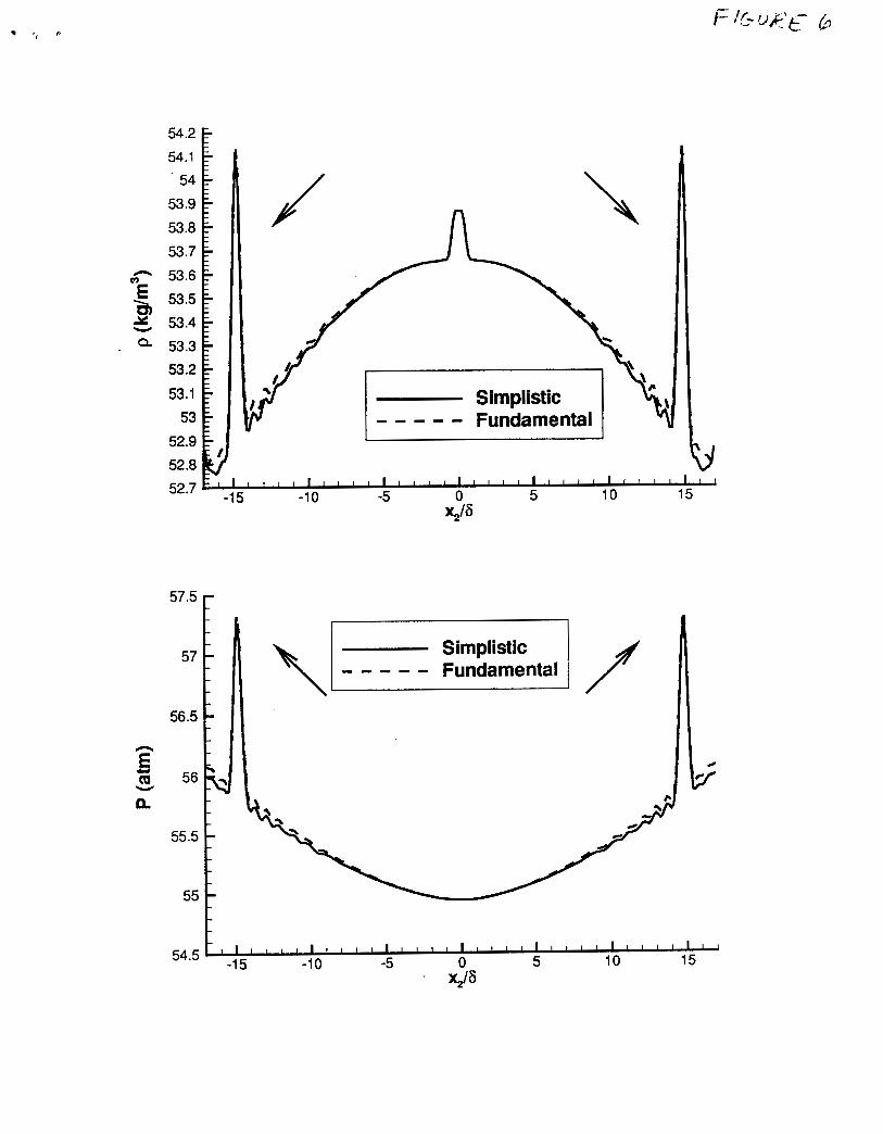
Previously developed characteristic-wave-based boundary conditions for multicomponent perfect gas mixtures are here extended to account for real gases. Following the general methodology, the characteristic boundary conditions are derived from the wave decomposition of the inviscid Eu- ler equations, and the wave amplitude variations are determined from the prescribed boundary conditions on the flow variables in conjunction with a general real gas equation of state. The formulation is tested on the propa- gation of acoustic waves which are shown to exit the computational domain with minimal reflection at a subsonic non-reflecting outflow boundary. The results from this formulation are compared with those of a simplistic sub- stitution of the real gas thermodynamic properties into previously derived, perfect gas characteristic relations, and it is shown that the simplistic sub- stitution is deficient, particularly for situations with species sources (rep- resenting mass emission and/or chemical reactions) in the computational domain.

Key words: partial differential equations, fluid mechanics, classical thermody-

namics and heat transfer.

CONTENTS 1. INTRODUCTION. 2. GENERAL EQUATIONS. 3. APPLICATION OF CHARACTERISTIC BOUNDARY CONDITIONS. 4. TESTS: PROPAGATION OF ACOUSTIC WAVES. 5. CONCLUSIONS. 6. APPENDIX A: DERIVATION OF THE COMPATIBILITY CONDITIONS USING THE TEIZI-

PERATURE AS A VARIABLE.

1. INTRODUCTION

Boundary conditions for fluid dynamic equations play a crucial role in determin-

ing the character of the solution. Since most fluid dynamic problems of practical

interest are complex, a solution to the set of differential equations and boundary

conditions is usually found numerically rather than analytically. For these types of

solutions Poinsot and Lele [l] distinguish between physical and numerical boundary

conclitions. The physical 1)ountiary conditions are those that arc intrinsically im-

posed by the problem to he solved and are associated with the differential equations.

The numerical boundary conditions are associated with the difference implementa-

tion of the differential equations and can be considered as compatibility relations

that must be added to the physical boundary conditions to palliate the uncertainty

in the variables that are not specified by the physical boundary conditions. Indeed,

for some types of physical problems described by the Euler or Navier-Stokes (NS)

equations, the number of necessary and sufEcient boundary conditions is smaller

than the number of primitive variables [2], [l], and the issue of the specification of

the remaining number of variables introduces the concept of numerical boundary

conditions. As Poinsot and Lele [l] note, these numerical boundary conditions must

satisfy the differential equations and also must prevent the introduction of spurious

numerical effects such as wave reflections from the boundaries of the computational

domain.

Boundary conditions derived from characteristic wave analysis were presented by

Kreiss [3], Engquist and Majda [4], Higdon [5], Thompson [6], Poinsot and Lele [l]

and Baum et al. [7]. Although this type of analysis is consistent with the Euler

equations, it does not seem applicable to the NS equations which are not hyperbolic.

The essential idea of using a characteristic wave analysis for the NS equations is

discussed by Dutt [2] and is based on the fact that at high Reynolds number, Re,

the NS equations may be considered as an incompletely elliptic perturbation of the

Euler equations. Gustafsson and Sundstrom [8] note that while for finite Re the

NS equations cannot be classified as hyperbolic, elliptic or parabolic, for Re -+ co

the NS equations constitute a quasi-linear hyperbolic system. Therefore, at these

conditions the essence of the NS equations may he considered to be hyperbolic, with

the diffusive terms providing only 'corrections' to their hyperbolic behavior. This

crucial observation allowed Poinsot and Lele [1] to use Thompson's [6] derivation

of numerical boundary conditions for hyperbolic systems to derive a similar set for

the NS equations. When implemented for a variety of example problems, these

numerical boundary conditions proved robust and yielded solutions in agreement

with the expected physics of the problem. More recently, Baum et al. [7] extended

the work of Poinsot and Lele [l] to multicomponent reactive flow problems where

the new issue is that of the source terms in the mass fraction and energy equations.

Although not explicitly stated, this extension implicitly assumed that the mass

fractions and energy equations may also be an incompletely elliptic perturbation

of the Euler-type equations. This implication is correct since in the classical, low

pressure equations the molar and heat fluxes are proportional to (ScRe)-l and

(Pr Re)-l, respectively, where Sc is the Schmidt number and Pr is the Prandtl

number. These studies were all performed for fluids obeying the perfect gas law.

However, there are many practical applications where the fluid is not a perfect

gas. Such situations occur in high pressure reactive flows typical of rocket engines,

Diesel engines or gas turbine engines, as well as in fluid flowing in pipes laid on the

ocean floor. The importance of real gas equations of state (EOSs) was highlighted

by Shyue [9] in his development of the algorithm for compressible multicomponent

liquid-gas flow using the van der Waals EOS. The new algorithm was built on

a previous interface-capturing approach and focussed on accurate wave tracking

resolution, including shock tracking.

The present work is devot.ed t,o tht? tlcrivatiorl of accurate m c l consistent bound-

ary conditions for reactive flows where the fluid is a real gas. Section 2 is first

devoted to new aspects of the conservation equations that may be important for

real gases, and then to the derivation of the boundary conditions. This derivation

follows the method of Thompson [6], Poinsot and Lele [l] and Baum et al. [7]

whereby a local one-dimensional inviscid (LODI) set of equations, described at the

boundary in characteristic form, embodies the essential behavior at the boundary.

The wave amplitude variation in the characteristic wave formulation is then con-

sistently computed to satisfy the desired boundary conditions for a general real gas

EOS, and the viscous conditions are separately applied as in Poinsot and Lele [I].

In Section 3 we discuss the generic implementation of these boundary conditions

for typical problems encountered in fluid dynamics, and in Section 4 we test the

derived boundary conditions for three specific problems involving propagation of

acoustic waves. We compare the results of these calculations with those of similar

calculations where the results of Baum et al. [7] are simplistically used by replacing

in their final results the perfect gas thermodynamic quantities with equivalent real

gas quantities, and we show that the simplistic approach leads to numerical prob-

lems and inaccuracies. Finally, we summarize this work and offer further comments

in the Conclusion section.

2. GENERAL EQUATIONS

Harstad and Bellan [lo], [ll], [12] have derived the multicomponent conservation

equations for real gases, non ideal mixtures. These equations have the typical

form of the NS equations augmented by the species and energy equations, and by

? 6 OKONGY). HI.:LI,,W. A N D lms ' rm

the EOS, with the exception t,hat t,llc ciifiusive terms in the species and energy

equations now contain additional t,crms. In the species and energy equations, the

respective Fick mass diffusion and Fourier heat diffusion terms are now respectively

complemented by the Soret and Dufour terms representing the thermal diffusion

contribution. These conservation equations are

where t is the time, xj is the j t h coordinate, p is the mass density, uj is the j th

velocity component, T is the temperature, Y, is the mass fraction of species a (for

N species Yo = l) , p is the pressure and ET = E + 4uiui is the total energy

(internal energy, E , plus kinetic energy). Additionally, rii is the Newtonian viscous

stress tensor

N

where p is the mixture viscosity which is in general a function of the thermodynamic

state variables, J , is the molar flux and q I K is the Irwing-Kirkwood (subscript I K )

form of the heat flux [131. The Einstein summation convention (summation over

repeated indices) is used for i and j , but not over Greek indices cy and /3.

For example, in this general situation which includes thermal diffusion effects,

the molar and heat fluxes [14] for a binary mixture are given by

where D is the mass diffusivity, m, is the species molar weight, m = CaZ1 maXa

is the mixture molar weight, & is the universal gas constant, X;, is a thermal con-

ductivity (see below), CYD is the mass diffusion factor calculated from the fugacity,

N

%x, as

are the partial molar volume and the partial molar enthalpy, respectively, v and h

being the molar volume and molar enthalpy, respectively. Furthermore, the molar

volume is related to the density by v = m / p , and X , = mY,/m, is the species

molar fraction. The thermal conductivity X;, is defined in [ll] and [12] from

the transport matrix. It can be shown that X;, does not correspond to the kinetic

theory (subscript KT ) definition of the thermal conductivity in that lirn,,o X;, #

X,* but it is related to the thermal conductivity, X, through

where limp,o X = XKT as discussed in [ll] and [12]. Although currently there is no

information as to the functional form of with respect to the primary variables

(p,T,Y,) and/or its magnitude, Harstad and Bellan [ll], [12] have determined its

approximate value for the heptane-nitrogen pair from comparisons of numerical

predictions with a partial set of data; once this coefficient was determined, the

remaining part of the data set was used to validate the model.

Therefore, the general form of the flux matrix is

where the coefficients of this matrix can be identified from direct comparisons with

Eqs. 6-9. Clearly, it is difficult a priori to state what is the essential character

of these equations: parabolic, elliptic or hyperbolic. Since the present boundary

conditions derivation is intended to be valid at higher than atmospheric pressures,

and since the Soret and Dufour contributions are known to become progressively

more important with increasing pressure [15], the question arises as to whether

Dutt's [2] conditions regarding the form of the equations that may be treated with

the characteristic wave approach is still satisfied. It is outside the scope of this

work to prove that the condition of the incomplete elliptic perturbation is here

valid for the mass fractions and energy equations; instead, we base our inference

on a comparison with the familiar set of equations discussed by Baum et al. [7]. If

we can show that there is a set of variables for which the more general equations

including Soret and Dufour effects assume a form similar to the diffusion equations

based on the Fick and Fourier diffusive fluxes, then we will assume that the method

of Baum et a l . [7] remains valid.

An analytical diagonalization of the species and energy equations operators under

the quasi-steady, boundary layer assumptions yields eigenvalues of the transport

matrix [16], which for a binary mixture are an effective m a s diffusivity, D , f f , and

a thermal conductivity, & s f , quantifying departures from D and X

10

where i is the positive root of an algebraic equation, n = p/m is the molar density,

and C, is the molar heat capacity at constant pressure. In Eqs. 15 and 16 CYBK is

the Bearman-Kirkwood (subscript B K ) thermal diffusion factor corresponding to

the BK form of the heat flux ([13]). It can be shown that lim,,o CYIK # CYKT and

lim,,o CYBK = Q K T , and that [12]

C X I K and CYBK are the new transport coefficients that are introduced by the Soret (in

the molar fluxes) and the Dufour (in the heat flux) terms of the transport matrix,

and are characteristic of the particular species pairs under consideration. Since a h

is a thermodynamic function, it is sufficient to know either CYIK or CXBK to have

the other thermal diffusion factor determined. The values of CYIK and CYBK will be

discussed in Section 4.

Since the second term in the right hand side of Eq. 15 and the third term in the

right hand side of Eq. 16 are both positive, it is apparent that the mass diffusivity

diminishes whereas the thermal conductivity is enhanced as thermal diffusion ef-

fects become important. Both effective coefficients are indeed positive defined (as

they physically should be), indicating that the set of new equations is of the type

discussed by Baum et al. [7], and that the concepts of Dutt [2] may still apply.

The same analysis can be extended to N component mixtures with similar results,

yic:lciillg N effective IIlikss cliffusivit,ics. However, it is irnrncdiatc!lv clear that tlm

ellipticity o f the system of equations is not determined by the c:f€octive dlffusivi-

ties which are always reduced compared to ideal mixtures (crg = 1) atmospheric

conditions (LYBK <<< 1) situations] because for non-ideal mixtures CXD < 1 and if

thermal diffusion effects are important one may have X1X2aiK&nD< comparable

to unity. What truly determines the level of ellipticity of the system is X,ff which

may possibly reach large values compared to X. Calculations performed with this

model [12] for heptane-nitrogen in the present range of (p , T ) (see Section 4) yielded

X,ff = O(X). Based on this circumstantial evidence it is still relevant to proceed

with the derivation of relations based on characteristic lines in order to analyze the

fate of waves crossing the boundary of a computational domain. However, we note

that because of the enhanced value of X, the ellipticity of the system of equations

does increase with increasing pressure, and depending on the values of the thermal

diffusion factors the essentially hyperbolic behavior of the system may be lost.

As in Poinsot and Lele [l] and Baum et al. [7], we start by analyzing the Eu-

ler equations] which contain the needed characteristic behavior at the boundaries.

Whereas in principle the entire enlarged Navier-Stokes equations should be ana-

lyzed, in fact the Euler equations alone provide the characteristic behavior of the

solution and therefore they are analyzed hereafter.

2.1. Euler Equations

The conservative form of the Euler equations augmented by the species and

energy equations is

where ET is the total energy per unit mass. This is a system of N + 5 differential

equations in the three-dimensional case.

The pressure is given by an EOS, a state being uniquely specified by the internal

energy E , the density and the mass fractions

d p d p duj - - + + j - + p - - 0 , at dXj d X j

where the speed of sound, c, is given by

(for brevity, the subscript Y, on a derivative denotes that all the mass fractions

are held constant). We chose here to develop the characteristic wave relationships

based on the pressure rather than on the temperature because waves are directly

related to p rather than T , making the former variable the prime choice. We present

in Appendix A an equivalent derivation based on TI similar to that of Baum et al.

(71.

i-)E p a ~ j i3E - + "

at axj axi + uj- = 0 ,

by substituting

and a similar expression for d E / % into Eq. 29. The internal energy derivatives

appearing in Eq. 30 can be computed from the EOS, as described below.

2.1.1. Real Gas Relations

The EOS, assumed here to have the most general form p = p ( T , v , YI, . . . , YN) , is

the relationship from which c as well as

all be calculated. From the EOS we can calculate the isentropic speed of sound

( F ) p,y,, ' (%) p,y, and (3) P,P7yQ can a#P

where K~ is the isentropic compressibility, which is related to the isothermal com-

pressibility KT

where

and C, is the molar heat capacity at constant pressure

with H being the enthalpy per unit mass and h being the enthalpy per mole,

h = m H

The molar heat capacity at constant volume is

In terms of the partial molar quantities, the enthalpy and molar volume are written

as

lo;

N N iV N

where the partial molar quantities were defined in Eq. 11. From the above thermo-

dynamic relationships one may now calculate the desired internal energy derivatives

and one can now observe that the speed of sound is in fact the isentropic speed of

sound

2.1.2. Perfect Gas Relations In the perfect gas case, the EOS is

where y = Cp/Cv

h, = Cp,,T,

v, = v ,

The internal energy is

(44)

(45)

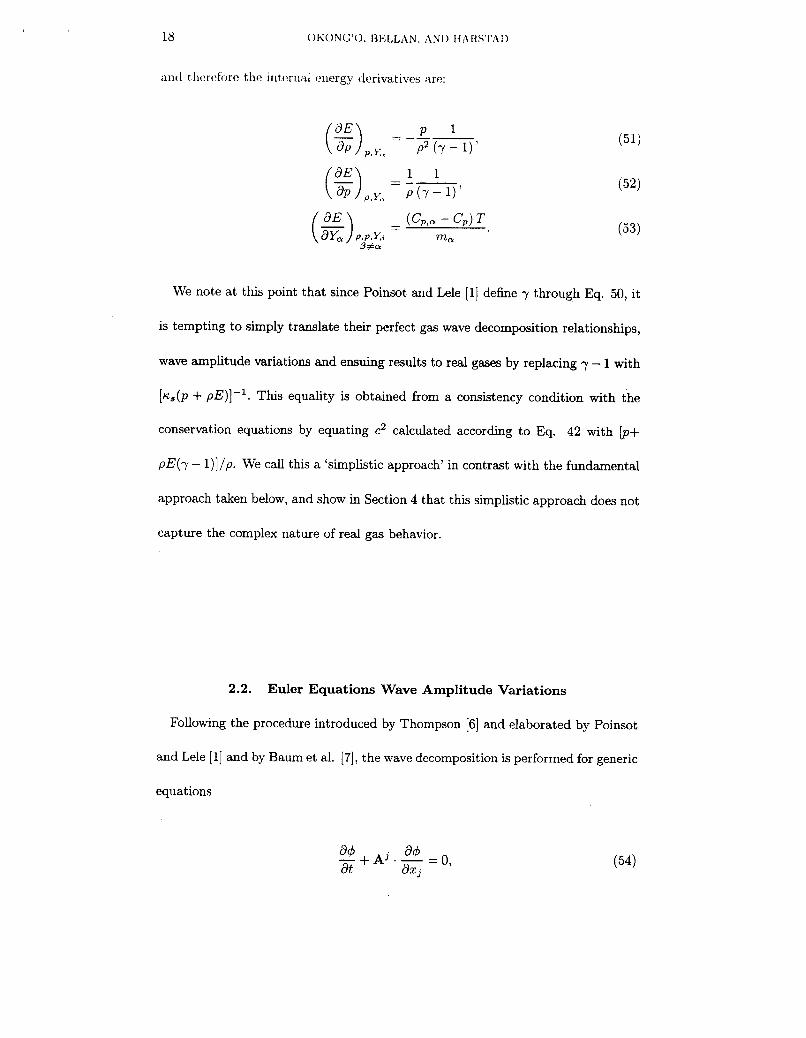
We note at this point that since Poinsot and Lele [l] define y through Eq. 50, it

is tempting to simply translate their perfect gas wave decomposition relationships,

wave amplitude variations and ensuing results to real gases by replacing y - 1 with

[ ~ ~ ( p + pE)]”. This equality is obtained from a consistency condition with the

conservation equations by equating c2 calculated according to Eq. 42 with [p+

pE(y - l)]/p. We call this a ‘simplistic approach’ in contrast with the fundamental

approach taken below, and show in Section 4 that this simplistic approach does not

capture the complex nature of real gas behavior.

2.2. Euler Equations Wave Amplitude Variations

Following the procedure introduced by Thompson [6] and elaborated by Poinsot

and Lele [I] and by Baum et al. [7], the wave decomposition is performed for generic

equations

and Aj are matrices:

r 1

0

0

0

0

0

0

0

U j

...

...

...

...

...

...

The wave decomposition involves computing the eigenvalues and eigenvectors, and

from these the wave amplitude variations. For the sake of brevity and clarity,

we will present below only the analysis pertinent to A' and d+/dxl , referring to

boundary conditions across a surface of fixed 2 1 . A similar derivation is made for

the other two dimensions.

i u1 p 0 0 0 0 ... 0

0 0 U l O 0 0 ... 0

0 0 O U l O 0 ... 0

0 PC2 0 0 U1 0 ... 0

0 0 0 0 0 U 1 ... 0

A' =

its eigenvalues, Xi, are determined from

det(X1- A') = (X - 2 ~ 1 ) ~ ' ~ [(X - ~ 1 ) ' - c2 = 0 1

as

(57)

These eigenvalues represent either the velocities of sound waves moving in the

negative ( X , ) or positive ( X N + ~ ) directions along the 2 1 axis relative to the local

convection velocity, or the velocities of waves moving at the local convection velocity

(X2 to XN+4).

Associated with these eigenvalues are t.he left eigenvect,ors r! o f A' satisfying

1 . A' = X1:

r 1

The procedure is continued by computing the quantities Li from C; = Xildr$/dxl =

As pointed out by Poinsot and Lele [l], by consequence of their definition

(l3) at = - t i ,

and thus the Ci represent the time variation of the wave amplitude for each com-

ponent of the vector 4 , each Ci being associated with a wave having the speed

Xi . By manipulating the Ci one may influence the amplitude of waves crossing a

given boundary and in particular hope to suppress spurious, unphysical waves. We

note that, as mentioned above, diffusive terms are not included in this analysis and

neither are source/sink terms; the implicit assumption is that the ellipticity of the

equations plays a secondary role in determining the character of the solution at the

boundary.

2.3. Euler Equations Wave Decomposition

According to Poinsot and Lek 111, it is possible to find potential Ci values for

the more general case of the complete equations (see Section 4 below) by exploring

the simpler case of a LODI system of equations. These LODI relationships are only

used to find constraints between the dependent variables and the wave amplitude

variation at the domain boundaries.

To accomplish this analysis, the Euler equations are cast in terms of the wave

amplitude variations by first calculating the spatial derivatives in terms of the Li:

The LODI system for the primitive variables containing time- and XI-derivative

terms is recast in terms of the Ci as:

-+c3=0, au2

at

- + c4 = o , at

6% - + La+4 = 0; cr = 1, N . at

BOUNDARY CONDITIONS FOR blULTICOMPONENT REAL CAS MIXTURES 25

From the above Eqs. 78-83, one can find the conservative variables:

- at + Y,dl+ pda+* = 0; a = 1, N ,

L N + 5 - CI

where the di are groups of terms involving x1 derivatives that must be constrained

by conditions suppressing numerically spurious behavior across the x1 boundary.

For a perfect gas the energy equation becomes

3. APPLICATION OF CHARACTERISTIC BOUNDARY

CONDITIONS

In the previous section, wave decomposition was used to rewrite the time and

spatial derivatives in terms of wave amplitude variations. The implementation of

the method consists in determining the correct values of these wave amplitude

variations according to the nature of the problem to be solved. In this process we

distinguish between the outgoing waves which carry information from the interior

of the computational domain and which therefore are based on the solution of the

conservation equations, and the incoming waves which carry information from the

exterior of the domain to the region where the solution is sought; these incoming

waves are the origin of the spurious behavior that must be mitigated.

The implementation of the method consists in calculating the amplitude variation

of outgoing waves from the derivatives at the boundary, which are based on the in-

terior points, whereas the incoming wave amplitude variations are determined from

the boundary conditions. In the discussion that follows, it is assumed that waves

travelling in the 5 1 > 0 direction exit the computational domain. The definition of

incoming and outgoing waves is reversed if waves entering the domain have Xi < 0.

With this convention, at a (subsonic) boundary where 0 < u1 < c, the outgoing

wave amplitudes are computed from the interior points, whereas the incoming wave

amplitude (L1 corresponding to X1 = u1 - c ) is derived from the specified bound-

ary conditions. On the other hand, at a (subsonic) boundary where "c < u1 < 0,

the incoming wave amplitude variations are set to zero (meaning that there are

no waves), except for those that can be derived from the specified boundary con-

ditions, whereas the outgoing wave amplitude variation ( L N + 5 corresponding to

X N + ~ = u1 + c) is computed from the interior points.

3.1. Subsonic Slip-wall Boundary Conditions

At slip walls, the normal velocity is zero, i.e. u1 = 0. Then, from Eq. 79,

L1 = L N + 5 and the remaining wave amplitude variations are determined from the

interior points using Eqs. 67 - 71.

'8 Ot iONG'O. 13tCI,IJ~\N. AND IfARS'I'AD

3.2. Subsonic Non-reflecting Outflow Boundary Conditions

As discussed in Poinsot arld Lele [ 11, theoretically a non-reflecting condition could

be imposed by setting the amplitude of incoming waves to zero, i.e. C1 = 0.

However, this leaves the flow with no way to maintain its pressure. To mitigate t h s

unphysical condition, the pressure at 'infinity' is imposed through C1 = K ( p - pm)

with K = ( ~ ( 1 - M 2 ) c / L where 0 is a constant, il/l is the maximum Mach number

in the domain and L is a characteristic size of the domain. The value of 0 can be

adjusted to fit the requirement of the problem and an optimal value of 0.58 has

been proposed by Rudy and Strikwerda [17] and implemented by Poinsot and Lele

[l] in one of their example problems.

The remaining wave amplitude variations are determined from the interior points

using Eqs. 67 through 71.

3.3. Supersonic Outflow Boundary Conditions

In the supersonic case, all the waves are outgoing, so the wave amplitude varia-

tions are determined from the interior points using Eqs. 66 - 71.

4. TESTS: PROPAGATION OF ACOUSTIC WAVES

To test the implementation of the consistent boundary condition based on the

characteristic wave method we consider the one-dimensional propagation of an

acoustic wave in a two-hmensional domain.

The computations are performcxcl for a supercritical two-componcnt nitrogcn-

heptane flow using the Peng-Robinson EOS as in Miller et al. [la]:

RUT Am P =

( V - Bm) (u2 + 2vBm - BL) ' -

where A,,, and B, are given from mixing rules as

(97)

The thermodynamic properties are obtained through various derivatives and func-

tions of the Gibbs energy (G):

where the superscript 0 represents the 'low pressure' reference condition for the

integration as generally used in the departure function formalism described by

Prausnitz et al. [19]. Since the integral is ill defined for a zero pressure reference

condition, we choose po = lbar such that vu = &T/po. This leads to

h = G - T ( g ) = h o + p - & T + K 1 P A "

where ho is the reference molar enthalpy and Cp" = dho/dT is the reference molar

heat capacity,

The conservation equations for the binary heptanenitrogen mixture are those of

Section 2 with heptane being species 1 and nitrogen being species 2.

All test cases below pertain to a two-dimensional domain ( 2 1 , z 2 ) of respective

dimensions L1 = 0.2 m and L2 = 232 m. The initial condition specifies uniform

and the density is calculated from the EOS. These initial conditions lead to two

waves, each propagating toward one boundary. We test the validity of the boundary

conditions implementation by computing three subsonic ( M , = 0.4) cases with

a1 = 0.1, u2 = 5.678, b = 6 . 8 5 9 ~ T = 600K and p , = 60 atm. Also evaluated

is the simplistic approach whereby the term - is replaced by - f p in the

characteristic form of the energy equation derived from the perfect gas formulation

[ l ] , and Lcg = ,& = 0 for the mass fractions. For each of the test cases, we compare

the predictions of the simplistic approach with those of the fundamental approach

derived here.

1 7 - 1 P C 2

The numerical scheme in the present simulations uses fourth-order Runge-Kutta

time integration and eighth-order finite-differencing, and the resolution is 50 x 232

points. Periodic conditions are employed in the x1 direction, and subsonic non-

reflecting outflow conditions are used with null mass fraction gradient in the x2

direction. The viscous conditions are applied as recommended by Poinsot and Lele

[l]: for the subsonic outflow, the gradients of the heat flux and of the shear stresses

normal to the boundary are set to zero.

Test 1: The first case has. an initially uniform condition for tllc mass fraction

( a : ~ = 0 ) with 111 =145 m/s. Figure 1 shows the density and pressure before the

waves reach the boundaries ( N t i m e is the number of time steps), whereas Fig. 2

shows them after the wave has reached the boundaries. As displayed in the figures,

both p and p remain constant, as expected; the small high frequency oscillations

can be attributed to the high-order (eighth-order) finite-differencing. We note, how-

ever, that the fundamental characteristic condition derived herein shows minimal

reflection, in contrast to the simplistic approach result where the reflected waves

can clearly be discerned.

Test 2: The second case has an initially linear mass fraction (a3 = 0.2) with

Z L ~ =137 m/s. The results are depicted in Figs. 3 and 4 where it is clear that the

results are similar to Test 1: minimal reflection is obtained using the fundamental

approach whereas there are spurious reflections in the simplistic approach. The

p profile remains linear at these early times because the diffusional characteristic

time is considerably larger than the times at which the solution is illustrated. The

acoustic time scale is t , = O.5L2/aS N 3.2 x lov4 s whereas the diffusional time

scale estimated from the centerline values of the solution is t D = 0 . 5 L ~ / [ p D CY^

( a Y h / a ~ ) ] N 0.531 S.

Test 3: The third case has the same initial condition as the first, but has a

time-varying mass fraction resulting from a finite heptane mass source term having

a Gaussian profile. This mass source is intended to mimic features of mass sources

that would arise from chemical reactions or the mass emission (not necessarily evap

oration, since at supercritical conditions there is only a single phase) from chunks

of supercritical fluid (usually modeled as droplets) in a spray. Due to this h e p

t,allo mass source term, thc Inass fract,ion is increasing with time shown in Fig.

5 whoro the two lines plot,ted correspond to the time stations of t,he density and

pressure profiles illustrated in Figs. 6 and 7. As in Tests 1 and 2, the fundamental

compatibility conditions based on the characteristic wave analysis allow the waves

to exit the boundary, whereas the simplistic approach exhibits significant reflec-

tion. Just as important, but different from Tests 1 and 2, the density and pressure

profiles from the two boundary conditions do not overlap before the waves reach

the boundary. The discrepancy is particularly notable at the boundary, where the

density profile computed using the fundamental approach relaxes smoothly but the

simplistic approach leads to a sharply increasing gradient. These results show that

for multicomponent fluids the nature of the solution is affected by the simplistic

approach not only at the boundaries, but also in the entire domain.

5. CONCLUSIONS

Consistent boundary conditions based on characteristic wave analysis were here

derived for multicomponent flows governed by real gas equations of state. The

governing equations account not only for departures from the perfect gas equation

of state, but also for mixture non-ideality and for thermal diffusion effects. The

characteristic wave analysis is based on the inherent assumption that the elliptic

terms act only as corrections to the essentially hyperbolic operator. Thus, diffu-

sional terms are not part of the consistent boundary condition analysis, but are

used in the governing equations once a solution is sought. It has been pointed out

that, based on the results of a diagonalization of the species and energy equations

operators, the condition of weak ellipticity, which underlines this analysis, may

not. always be satisfied when therlrlal diffusion r?ffocts are important. Wllether this

condition is satisfied tlepends on the ( p . T , k , ) regime and on the species under

consideration, determining the value of the effective thermal conductivity.

The conditions derived herein have been tested on the one-dimensional propaga-

tion of acoustic waves in a two-dimensional domain by using subsonic non-reflecting

boundaries for a binary nitrogen-heptane mixture at 600 K and 60 atm. Moreover,

boundary conditions derived by simplistically replacing the gas constant in the re-

sults of Baum et al. [7] with its equivalent real gas quantities have also been tested.

It is shown that whereas using the fundamental analysis results in the acoustic

waves properly passing through the boundaries without reflections, the use of the

simplistic approach yields significant reflections at the boundaries. Most discrep

ancies occurred when a source term was added to the mass fraction equations; in

this case, additional to the reflections at the boundaries, the solution within the

entire domain was affected by the simplistic approach, exhibiting differences from

that found using the fundamental approach.

6. APPENDIX A: DERIVATION OF THE COMPATIBILITY

CONDITIONS USING THE TEMPERATURE AS A VARIABLE

A mathematical development similar to that of Baum et al. [7] is given here for

readers who find that in their application the natural primitive variable is T rather

than p . The basic equations in conservative form are

d e a F . - -+.'+c=o at d X j

BOUNDARY CONDITIONS FOR bIIILTICObIPONENT REAL GAS bIIX'TURES 35

where

where the S 's are source terms (e.g. Miller and Bellan (201) with SI = E, SI,^. As

in Baum et a l . [7] and above, the characteristic form of the equations is obtained

from their primitive form

where

and Aj = P-l . Q j , C = P-' ' where P E dG:/dU and Q j E dFj/dU. The

matrix P has the same form as in Baum et al. [7] with the diagonal elements equal

and differing from Baum et al. [7]

with

We note that for a perfect gas, matrices P and Aj coincide with those obtained by

Baum et al. [7]. Following the derivation of Baum et al. [7] for the boundary whose

normal is in the j = 1 direction, we calculate the eigenvalues of A’. However, for

notational convenience, here we order the eigenvalues differently so as to obtain a

38 OKONC'O. BELLAN, AND HI\IWTAD

more compact notation when specifying the vector and matrix elements

The first two eigenvalues correspond to the acoustic modes, the third to the entropy

mode, the fourth and fifth to the transverse velocities u2 and u3, and finally the

last a last ones correspond to the mass fraction modes. Corresponding to the

eigenvalues, left eigenvectors are used as rows of a matrix S', while (S')-' has as

its columns the right eigenvectors of A'. The elements of (S1)-' are (Sl),' = 6,j

except

(s1);:+5 = --- , (S1)$ = 0. P va a v ma

The mode amplitude variations are defined using the left eigenvectors through

where M' P.(S')-l. The explicit expressions for C and 2 are:

LC1 = (u1 + c) - + pc- [::1 E::] '

40

arid

L3 - = a@+&) - 1 E' u1 1 2 1 c 2 c 2 c 1 ) ~ ~ - %.] C , ax1

- - -(- + l ) t l + "(2 -

- = "(-131 + zL2 - L3) + p L 5 , u3 1 1 L5 =

1 c2 2

where

= -(- - -)' 1 HT 211

2 c2 c

These relationships which are valid for real gases and non-ideal mixtures are equiv-

alent to those of Baum et al. [7] which were derived for perfect gases and ideal

mixtures only.

ACKNOWLEDGMENT

This study was conducted at the Jet Propulsion Laboratory (JPL) and spon-

sored jointly by the Air Force Office of Scientific Research under the direction of

Dr. Julian Tishkoff and by the Army Research Office under the direction of Dr.

David Mann under an interagency agreement with the National Aeronautics and

Space Administration. The computational resources were provided by the JPL

Supercomputing Center.

, 42

REFERENCES

1 . T . .I. Puinsot and S. K. Lele, Boundary conditions for direct simulations u f compressible viscous

flows, . J . Comp. Phgs. 101, 10-1 (1992).

2. P. Dutt, Stable boundary conditions and difference schemes for Navier-Stokes equations, SIAM

J . Numer. Anal. 25(2), 245 (1988).

3. H.-0 . Kreiss, Initial boundary value problems for hyperbolic systems, Commun. Pure Appl.

Math. 23, 277 (1970).

4. B. Engquist and A. Majda, Absorbing boundary-conditions for numerical-simulation of waves,

Math. Comput. 31(139), 629 (1977).

5. R. L. Higdon, Initial-boundary value problems for linear hyperbolic systems, SIAM Rev. 28(2),

177 (1986).

6. K. Thompson, Time dependent boundary conditions for hyperbolic systems, J . Comp. Phys.

68, 1 (1987).

7. M. Baum, T. Poinsot, and D. Thhvenin, Accurate boundary conditions for multicomponent

reactive flows, J. Comp. Phys. 116, 247 (1994).

8. B. Gustafsson and A. Sundstrom, Incompletely parabolic problems in fluid dynamics, SIAM

J. Appl . Math. 35(2), 343 (1978).

9. K.-M. Shyue, A fluid-mixture type algorithm for compressible multicomponent flow with van

der Waals equation of state, J . Comp. Phys. 156, 43 (1999).

10. K. Harstad and J . Bellan, Isolated fluid oxygen drop behavior in fluid hydrogen at rocket

chamber pressures, Int. J . Heat Mass nansfer 41, 3537 (1998).

11. K. Harstad and J. Bellan, A validated all-pressure fluid drop model for binary mixtures:

heptane in nitrogen, AIAA 99-206, Joint AIAA/ASME/SAE Propulsion Meeting (1999).

12. K. Harstad and J. Bellan, An all-pressure fluid drop model applied to a binary mixture:

heptane in nitrogen, in press Int. J. of Multiphase Flow (1999).

13. S. Sarman and D. J. Evans, Heat flux and mass diffusion in binary Lennard-Jones mixtures,

Phys. Rev. A45(4), 2370 (1992).

14. J . Keizer, Statistical thermodynamics of nonequdibrium processes (Springler-Verlag, New

York, 1987).

15. I t . D. Bird, W. E. Stewart, and E. N . Lightfoot, 'fiansporl Phenontenu (,JcJhn Wiley and Sons,

1960).

16. K . Harstad and J. Bellan, The Lewis number under supercritical conditions, Int. J . Heat Mass

Pansfer 42, 961 (1999).

17. D. H. Rudy and J. C. Strikwerda, A nonreflecting outflow boundary-conditions for subsonic

Navier-Stokes calculations, J . Comp. Phys. 38(1), 55 (1980).

18. R. S. Miller, K. Harstad, and J. Bellan, Direct numerical simulations of supercritical fluid

mixing layers applied to heptane-nitrogen, submitted to J . Fluid Mech. (1999).

19. J. Prausnitz, R. Lichtenthaler and E. de Azevedo, Molecular thermodynamics for fluid-phase

equilibrium (Prentice -Hall, Inc., 1986).

20. R. S. Miller, and J . Bellan, Direct numerical simulation of a confined three-dimensional gas

mixing layer with one evaporating hydrocarbon-droplet-laden stream, J. Fluid Mech. 384,

293-338 (1999)

44

FIG. 1. Wave profile before reaching boundary, uniform mass fraction, t = 2.85 X

N~~~~ = 141

FIG. 2. Wave Profile after reaching boundary, uniform mass fraction, t = 3.80 X

10-4s, Ntime = 187

FIG. 3. Wave profile before reaching boundary, linear maSS fraction, t = 2.01 x lo-%, N~~~~ = 104

209 FIG. 4. Wave profile after reaching boundary, linear mass fraction, t = 4.03 X 10e4s, Ntine =

FIG. 5. Mass fraction from heptane mass source

FIG. 7. Wave profile after reaching boundary, heptane mass source, t = 3.80 X 10-49, Ntime = 182

54.4 F 54.3

54.2

54.1

54

53.9

53.8

53.7

53.6

53.5

53.4

53.3

53.2

53.1

53 -1 5

Simplistic ""_ Fundamental

-1 0 -5 5 10 15

Simplistic ""_ Fundamental

-1 0 -5 0 5 10 15 318

Q

61

60

59

58

57

56

55

54

53

52

51

50

49

48

47

L

Simplistic ""_ Fundamental

-1 5 -1 0 -5 0 5

61.6

61.4

61.2

a 60.6

60.4

60.2

60

Simplistic -"" Fundamental

- 10 15

L

59.8

Q

61

60

59

58

57

56

55

54

53

52

51

50

49

48

47

Simplistic ""- Fundamental

0.575

0.57

0.565

0.56

0.555 f

0.55

0.545

0.54

0.535

0.53

54.2 54.1

54 53.9 53.8 53.7

n 53.6 3 53.5 m 5 53.4 53.3 53.2 53.1

53 52.9 52.8 52.7

n E

e w U tu

/ \

Simplistic Fundamental

57

56.5

56

55.5

55

54.5

d t

Simplistic ""_ Fundamental


Recommended