Constant proportion harvest policies: Dynamic implications in the Pacific halibut and Atlantic cod fisheries Abdul-Aziz Yakubu a,⇑ , Nianpeng Li a , Jon M. Conrad b , Mary-Lou Zeeman c a Department of Mathematics, Howard University, Washington, DC 20059, United States b Charles H. Dyson School of Applied Economics and Management, Cornell University, Ithaca, NY 14853, United States c Department of Mathematics, Bowdoin College, Brunswick, ME 04011, United States article info Article history: Received 28 December 2009 Received in revised form 28 March 2011 Accepted 15 April 2011 Available online 5 May 2011 Keywords: Allee effect Compensatory and overcompensatory dynamics Sustainability abstract Overfishing, pollution and other environmental factors have greatly reduced commercially valuable stocks of fish. In a 2006 Science article, a group of ecologists and economists warned that the world may run out of seafood from natural stocks if overfishing continues at current rates. In this paper, we explore the interaction between a constant proportion harvest policy and recruitment dynamics. We examine the discrete-time constant proportion harvest policy discussed in Ang et al. (2009) and then expand the framework to include stock-recruitment functions that are compensatory and overcompen- satory, both with and without the Allee effect. We focus on constant proportion policies (CPPs). CPPs have the potential to stabilize complex overcom- pensatory stock dynamics, with or without the Allee effect, provided the rates of harvest stay below a threshold. If that threshold is exceeded, CPPs are known to result in the sudden collapse of a fish stock when stock recruitment exhibits the Allee effect. In case studies, we analyze CPPs as they might be applied to Gulf of Alaska Pacific halibut fishery and the Georges Bank Atlantic cod fishery based on harvest rates from 1975 to 2007. The best fit models suggest that, under high fishing mortalities, the halibut fishery is vulnerable to sudden population collapse while the cod fishery is vulnerable to steady decline to zero. The models also suggest that CPP with mean harvesting levels from the last 30 years can be effective at preventing collapse in the halibut fishery, but these same policies would lead to steady decline to zero in the Atlantic cod fish- ery. We observe that the likelihood of collapse in both fisheries increases with increased stochasticity (for example, weather variability) as predicted by models of global climate change. Ó 2011 Elsevier Inc. All rights reserved. 1. Introduction Fisheries throughout the world are in crisis [5,7,9,11,16,22,23, 28,31,32]. In a recent paper, Ang et al. examine the degree of sub-optimality when fishery managers use the best constant pro- portion policy (CPP) instead of the optimal variable proportion pol- icy (VPP). Sub-optimality was measured relative to the maximized discounted net revenue in a single-species, discrete-time, unstruc- tured population model [1]. In their model, Ang et al. adopted a lo- gistic escapement function. They identified the best constant proportion policy and the best variable proportion policy for the Pacific halibut fishery in Gulf of Alaska in Area 3A (see Fig. 1). In this paper, we extend that framework to include discrete- time fisheries that exhibit compensatory stock dynamics, with and without the Allee effect (e.g. the Beverton–Holt and modified Beverton–Holt models) and overcompensatory stock dynamics with and without the Allee effect (e.g. the Ricker and modified Ricker models) [2–4,6,9–14,17–27,29–32]. We use the model framework to assess performance of harvested fisheries that vary in levels of compensation with and without depensation (Allee effect) under constant harvest regimes. It is known that both CPPs can stabilize complex behavior caused by overcompensatory dynamics but they may result in a sudden collapse of the fish stock when the Allee effect is present. In the absence of the Allee effect, our models show that, as the harvest fraction increases, yield (har- vest) first rises gradually to a maximum sustainable level and then declines continuously to zero. As case studies, we apply the theoretical model framework to Gulf of Alaska Pacific halibut fishery data from the International Pacific halibut Commission (IPHC) annual reports and Atlantic cod fishery data from the North East Fisheries Science Center (NEFSC) Reference Document [1,5,22]. The Gulf of Alaska Pacific halibut fishery data is for Area 3A (see Fig. 1) and that of the Atlantic cod fishery is for the Georges Bank (see Fig. 2). Our analy- sis indicate that under CPP, mean harvest rates of the last 30 years are effective at preventing collapse in the halibut fishery but 0025-5564/$ - see front matter Ó 2011 Elsevier Inc. All rights reserved. doi:10.1016/j.mbs.2011.04.004 ⇑ Corresponding author. E-mail addresses: [email protected](A.-A. Yakubu), [email protected](N. Li), [email protected](J.M. Conrad), [email protected](M.-L. Zeeman). Mathematical Biosciences 232 (2011) 66–77 Contents lists available at ScienceDirect Mathematical Biosciences journal homepage: www.elsevier.com/locate/mbs
Transcript
Mathematical Biosciences 232 (2011) 66–77
Contents lists available at ScienceDirect
Mathematical Biosciences
journal homepage: www.elsevier .com/locate /mbs
Constant proportion harvest policies: Dynamic implications in the Pacifichalibut and Atlantic cod fisheries
Abdul-Aziz Yakubu a,⇑, Nianpeng Li a, Jon M. Conrad b, Mary-Lou Zeeman c
a Department of Mathematics, Howard University, Washington, DC 20059, United Statesb Charles H. Dyson School of Applied Economics and Management, Cornell University, Ithaca, NY 14853, United Statesc Department of Mathematics, Bowdoin College, Brunswick, ME 04011, United States
a r t i c l e i n f o a b s t r a c t
Article history:Received 28 December 2009Received in revised form 28 March 2011Accepted 15 April 2011Available online 5 May 2011
Keywords:Allee effectCompensatory and overcompensatorydynamicsSustainability
0025-5564/$ - see front matter � 2011 Elsevier Inc. Adoi:10.1016/j.mbs.2011.04.004
Overfishing, pollution and other environmental factors have greatly reduced commercially valuablestocks of fish. In a 2006 Science article, a group of ecologists and economists warned that the worldmay run out of seafood from natural stocks if overfishing continues at current rates. In this paper, weexplore the interaction between a constant proportion harvest policy and recruitment dynamics. Weexamine the discrete-time constant proportion harvest policy discussed in Ang et al. (2009) and thenexpand the framework to include stock-recruitment functions that are compensatory and overcompen-satory, both with and without the Allee effect.
We focus on constant proportion policies (CPPs). CPPs have the potential to stabilize complex overcom-pensatory stock dynamics, with or without the Allee effect, provided the rates of harvest stay below athreshold. If that threshold is exceeded, CPPs are known to result in the sudden collapse of a fish stock whenstock recruitment exhibits the Allee effect. In case studies, we analyze CPPs as they might be applied to Gulfof Alaska Pacific halibut fishery and the Georges Bank Atlantic cod fishery based on harvest rates from 1975to 2007. The best fit models suggest that, under high fishing mortalities, the halibut fishery is vulnerable tosudden population collapse while the cod fishery is vulnerable to steady decline to zero. The models alsosuggest that CPP with mean harvesting levels from the last 30 years can be effective at preventing collapsein the halibut fishery, but these same policies would lead to steady decline to zero in the Atlantic cod fish-ery. We observe that the likelihood of collapse in both fisheries increases with increased stochasticity (forexample, weather variability) as predicted by models of global climate change.
� 2011 Elsevier Inc. All rights reserved.
1. Introduction
Fisheries throughout the world are in crisis [5,7,9,11,16,22,23,28,31,32]. In a recent paper, Ang et al. examine the degree ofsub-optimality when fishery managers use the best constant pro-portion policy (CPP) instead of the optimal variable proportion pol-icy (VPP). Sub-optimality was measured relative to the maximizeddiscounted net revenue in a single-species, discrete-time, unstruc-tured population model [1]. In their model, Ang et al. adopted a lo-gistic escapement function. They identified the best constantproportion policy and the best variable proportion policy for thePacific halibut fishery in Gulf of Alaska in Area 3A (see Fig. 1).
In this paper, we extend that framework to include discrete-time fisheries that exhibit compensatory stock dynamics, withand without the Allee effect (e.g. the Beverton–Holt and modifiedBeverton–Holt models) and overcompensatory stock dynamics
with and without the Allee effect (e.g. the Ricker and modifiedRicker models) [2–4,6,9–14,17–27,29–32]. We use the modelframework to assess performance of harvested fisheries that varyin levels of compensation with and without depensation (Alleeeffect) under constant harvest regimes. It is known that both CPPscan stabilize complex behavior caused by overcompensatorydynamics but they may result in a sudden collapse of the fish stockwhen the Allee effect is present. In the absence of the Allee effect,our models show that, as the harvest fraction increases, yield (har-vest) first rises gradually to a maximum sustainable level and thendeclines continuously to zero.
As case studies, we apply the theoretical model framework toGulf of Alaska Pacific halibut fishery data from the InternationalPacific halibut Commission (IPHC) annual reports and Atlanticcod fishery data from the North East Fisheries Science Center(NEFSC) Reference Document [1,5,22]. The Gulf of Alaska Pacifichalibut fishery data is for Area 3A (see Fig. 1) and that of theAtlantic cod fishery is for the Georges Bank (see Fig. 2). Our analy-sis indicate that under CPP, mean harvest rates of the last 30 yearsare effective at preventing collapse in the halibut fishery but
endanger the cod fishery. Stochastic versions of the model indicatethat the likelihood of the collapse of both halibut and cod fisheriesincreases with increased stochasticity in the fish environment.
The rest of the paper is organized as follows. In Section 2, weintroduce the general model for regulation with a CPP and we de-fine compensatory, overcompensatory and depensatory (Allee ef-fect) recruitment dynamics. In Section 3 we explore theinteractions between recruitment dynamics and CPP. Section 4examines the Gulf of Alaska halibut fishery, Section 5 analyzesthe Georges Bank cod fishery, and concluding remarks are pre-sented in Section 6.
2. Harvested fisheries population model
In this section, we introduce the single species discrete-timefish stock mathematical model for regulation with a CPP. At thestart of year t, we let x(t) denote the fish stock (biomass) and y(t)the total allowable catch (TAC). The total allowable catch is thefraction, 0 < a < 1, of the estimated stock. That is,
yðtÞ ¼ axðtÞ: ð1Þ
Since the harvesting fraction is constant a 2 (0,1), we refer toy(t) = ax(t) as the constant proportion policy (CPP). The CPP is trans-parent, easily implemented and historically acceptable to fishers[1].
At the start of year t, the escapement is defined as
sðtÞ ¼ xðtÞ � yðtÞ ¼ ð1� aÞxðtÞ: ð2Þ
We assume that reproduction occurs halfway through the seasonand is characterized by the recruitment function
f ðsðtÞÞ ¼ sðtÞgðsðtÞÞ; ð3Þ
where the per-capita growth function, g : ½0;1Þ ! ½0;1Þ, is as-sumed to be a continuously differentiable function.
The dynamics of the harvested stock are then described by thedeterministic, discrete-time, unstructured population model
xðt þ 1Þ ¼ ð1�mÞsðtÞ þ f ðsðtÞÞ; ð4Þ
where m 2 (0,1) is the (constant) natural mortality rate. Theassumption about the timing of recruitment allows compressionof the age-structure of the model so that one can work with a min-imum number of equations. There are two terms for the populationdynamics: survival of mature fish (1 �m)s(t), and recruits to thepopulation, f(s(t)).
Using Eqs. (2) and (3), Model (4) becomes the exploited fishpopulation model,
The set of iterates of the function G is equivalent to the set of stocksequences generated by Model (5). Note that when the per capitagrowth rate is the logistic model and
gðxðtÞÞ ¼ r 1� xðtÞK
� �;
then Model (5) reduces to that of Ang et al. [1].The fish population is said to be persistent if lim t?1Gt(x) > 0 for
all x > 0. Moreover, the population is said to be uniformly persistentwhen there exists a constant g > 0 such that limt?1Gt(x) P g for allx > 0.
In Section 3 we analyze the behavior of Model (5) under CPP, forstock populations exhibiting compensatory, overcompensatoryand/or depensatory (Allee effect) recruitment dynamics. First, wedefine these terms in Section 2.1.
2.1. Compensatory, overcompensatory and depensatory vital rates
The per-capita growth rate, g, is said to be compensatory if for alls P 0
dgðsÞds
< 0;
df ðsÞds
> 0
and
lims!1
f ðsÞ ¼ g > 0:
When g is compensatory the decline in the per-capita growth ratewith density exactly compensates for the increase in density so thatthe net growth rate is asymptotically constant [3].
For example, when f is the classic monotone Beverton–Holtstock recruitment model,
f ðsÞ ¼ as1þ bs
; ð6Þ
where the intrinsic growth rate, a, and the scaling parameter, b, arepositive constants, then g is compensatory. If a > 1, then f0(0) > 1,the Beverton–Holt model has a globally attracting equilibrium pointat x1 ¼ a�1
b 2 ð0;1Þ and all positive initial conditions converge to x1monotonically under f iterations.
The per-capita growth rate, g, is said to be overcompensatoryif
lims!1
f ðsÞ ¼ 0:
When g is overcompensatory an increase in s is more than compen-sated for by a decrease in g(s) at high densities [3].
For example, when f is the classic Ricker stock recruitmentmodel,
f ðsÞ ¼ ase�bs; ð7Þ
where the intrinsic growth rate, a, and the scaling parameter b arepositive constants, then g is overcompensatory [29–32]. If a > 1,then f0(0) > 1 and the one-humped Ricker model has a positive equi-librium point at x1 ¼ ln a
b 2 ð0;1Þ . Depending on the model param-eters, the Ricker model can exhibit oscillatory and chaoticdynamics.
When
dgðsÞds
> 0
for some s > 0, then the per-capita growth rate g is said to exhibitdepensation or the Allee effect [3].The Allee effect describes a positiverelation between population density and the per capita growth rateof species. In the presence of the Allee effect, there is a decrease inpopulation growth rate at low population sizes, and the effect usu-ally saturates or disappears as populations get larger. Presence ofthe Allee effect in populations may be due to any number of causes.In some species, reproduction or finding a mate is increasingly dif-ficult as the population density decreases [3–6,11,14,16,19,25].
For example, when f is either the modified Beverton–Holt stockrecruitment model,
f ðsÞ ¼ as2
1þ bs2 ; ð8Þ
or the modified Ricker stock recruitment model,
f ðsÞ ¼ as2e�bs; ð9Þ
g is depensatory.Scramble and contest competition are two extreme forms of
intraspecific competition for resources [21]. Systems that exhibitscramble competition try to support all individuals including thosewho are non-reproductive. In scramble competition, the resources
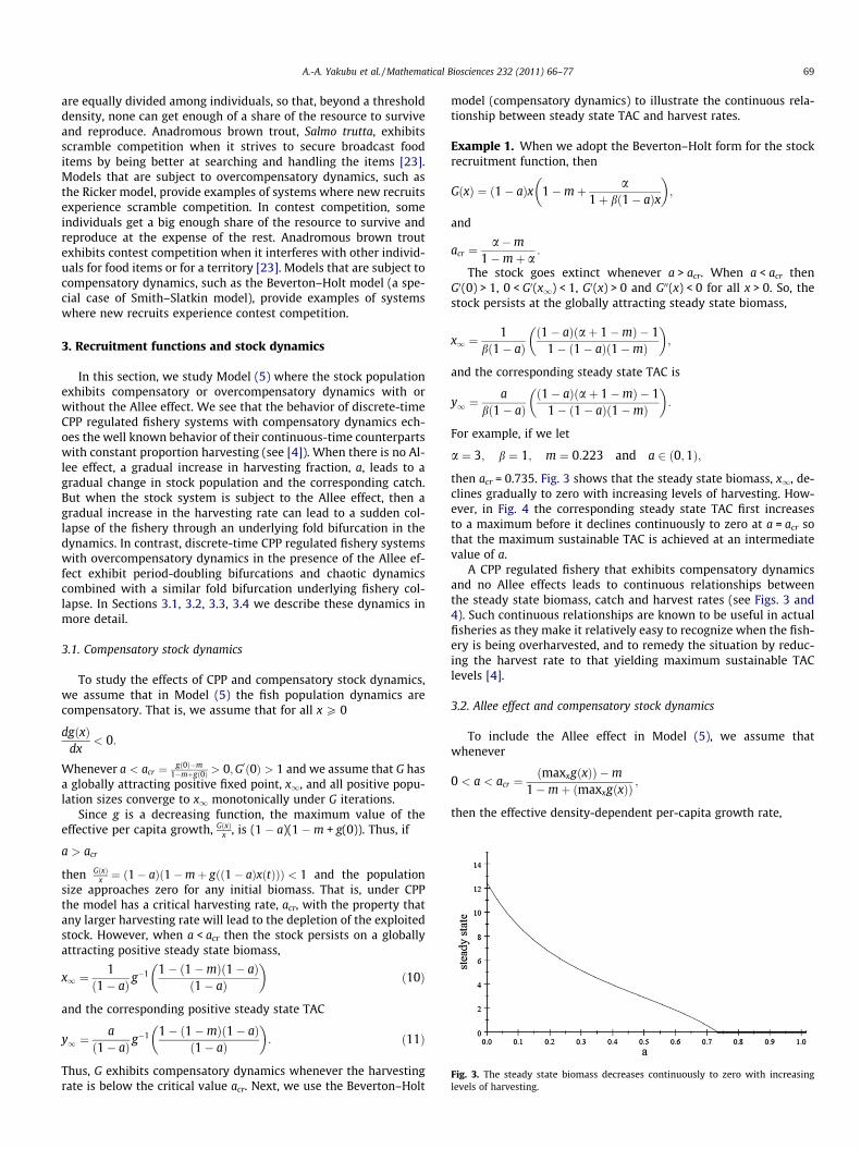
Fig. 3. The steady state biomass decreases continuously to zero with increasinglevels of harvesting.
are equally divided among individuals, so that, beyond a thresholddensity, none can get enough of a share of the resource to surviveand reproduce. Anadromous brown trout, Salmo trutta, exhibitsscramble competition when it strives to secure broadcast fooditems by being better at searching and handling the items [23].Models that are subject to overcompensatory dynamics, such asthe Ricker model, provide examples of systems where new recruitsexperience scramble competition. In contest competition, someindividuals get a big enough share of the resource to survive andreproduce at the expense of the rest. Anadromous brown troutexhibits contest competition when it interferes with other individ-uals for food items or for a territory [23]. Models that are subject tocompensatory dynamics, such as the Beverton–Holt model (a spe-cial case of Smith–Slatkin model), provide examples of systemswhere new recruits experience contest competition.
3. Recruitment functions and stock dynamics
In this section, we study Model (5) where the stock populationexhibits compensatory or overcompensatory dynamics with orwithout the Allee effect. We see that the behavior of discrete-timeCPP regulated fishery systems with compensatory dynamics ech-oes the well known behavior of their continuous-time counterpartswith constant proportion harvesting (see [4]). When there is no Al-lee effect, a gradual increase in harvesting fraction, a, leads to agradual change in stock population and the corresponding catch.But when the stock system is subject to the Allee effect, then agradual increase in the harvesting rate can lead to a sudden col-lapse of the fishery through an underlying fold bifurcation in thedynamics. In contrast, discrete-time CPP regulated fishery systemswith overcompensatory dynamics in the presence of the Allee ef-fect exhibit period-doubling bifurcations and chaotic dynamicscombined with a similar fold bifurcation underlying fishery col-lapse. In Sections 3.1, 3.2, 3.3, 3.4 we describe these dynamics inmore detail.
3.1. Compensatory stock dynamics
To study the effects of CPP and compensatory stock dynamics,we assume that in Model (5) the fish population dynamics arecompensatory. That is, we assume that for all x P 0
dgðxÞdx
< 0:
Whenever a < acr ¼ gð0Þ�m1�mþgð0Þ > 0;G0ð0Þ > 1 and we assume that G has
a globally attracting positive fixed point, x1, and all positive popu-lation sizes converge to x1 monotonically under G iterations.
Since g is a decreasing function, the maximum value of theeffective per capita growth, GðxÞ
x , is (1 � a)(1 �m + g(0)). Thus, if
a > acr
then GðxÞx ¼ ð1� aÞð1�mþ gðð1� aÞxðtÞÞÞ < 1 and the population
size approaches zero for any initial biomass. That is, under CPPthe model has a critical harvesting rate, acr, with the property thatany larger harvesting rate will lead to the depletion of the exploitedstock. However, when a < acr then the stock persists on a globallyattracting positive steady state biomass,
x1 ¼1
ð1� aÞ g�1 1� ð1�mÞð1� aÞ
ð1� aÞ
� �ð10Þ
and the corresponding positive steady state TAC
y1 ¼a
ð1� aÞ g�1 1� ð1�mÞ 1� að Þ
ð1� aÞ
� �: ð11Þ
Thus, G exhibits compensatory dynamics whenever the harvestingrate is below the critical value acr. Next, we use the Beverton–Holt
model (compensatory dynamics) to illustrate the continuous rela-tionship between steady state TAC and harvest rates.
Example 1. When we adopt the Beverton–Holt form for the stockrecruitment function, then
GðxÞ ¼ ð1� aÞx 1�mþ a1þ bð1� aÞx
� �;
and
acr ¼a�m
1�mþ a:
The stock goes extinct whenever a > acr. When a < acr thenG0(0) > 1, 0 < G0(x1) < 1, G0(x) > 0 and G00(x) < 0 for all x > 0. So, thestock persists at the globally attracting steady state biomass,
x1 ¼1
bð1� aÞð1� aÞðaþ 1�mÞ � 1
1� ð1� aÞð1�mÞ
� �;
and the corresponding steady state TAC is
y1 ¼a
bð1� aÞð1� aÞ aþ 1�mð Þ � 1
1� ð1� aÞð1�mÞ
� �:
For example, if we let
a ¼ 3; b ¼ 1; m ¼ 0:223 and a 2 ð0;1Þ;
then acr = 0.735. Fig. 3 shows that the steady state biomass, x1, de-clines gradually to zero with increasing levels of harvesting. How-ever, in Fig. 4 the corresponding steady state TAC first increasesto a maximum before it declines continuously to zero at a = acr sothat the maximum sustainable TAC is achieved at an intermediatevalue of a.
A CPP regulated fishery that exhibits compensatory dynamicsand no Allee effects leads to continuous relationships betweenthe steady state biomass, catch and harvest rates (see Figs. 3 and4). Such continuous relationships are known to be useful in actualfisheries as they make it relatively easy to recognize when the fish-ery is being overharvested, and to remedy the situation by reduc-ing the harvest rate to that yielding maximum sustainable TAClevels [4].
3.2. Allee effect and compensatory stock dynamics
To include the Allee effect in Model (5), we assume thatwhenever
0 < a < acr ¼ðmaxxgðxÞÞ �m
1�mþ ðmaxxgðxÞÞ ;
then the effective density-dependent per-capita growth rate,
0.0 0.1 0.2 0.3 0.4 0.5 0.6 0.7 0.8 0.9 1.00.0
0.5
1.0
1.5
2.0
a
TAC
Fig. 4. TAC first increases to a maximum before it declines to zero with increasingvalues of a.
increases continuously from positive values smaller than 1 to amaximum value greater than 1 and then decreases continuouslyto positive values smaller than 1 as the stock size is furtherincreased.
By our assumptions, when a < acr then G has two positive fixedpoints, the Allee threshold xA
1 and a positive steady state x1 > xA1.
All initial population sizes in the interval ½0; xA1Þ converge to {0} un-
der G iterations. Furthermore, we assume that all positive initialpopulation sizes greater than xA
1 converge monotonically to theattracting steady state biomass x1. Our assumptions guarantee astrong Allee effect and compensatory dynamics in Model (5) when-ever the harvesting rate is below the critical value acr.
In the presence of the Allee effect, whenever the harvesting ratea > acr, then
GðxÞx
< 1
for all x > 0 and the steady state biomass and TAC both collapse tozero. However, whenever the harvesting rate a < acr, then there ispersistence of the fish population at high initial stock levels.
Example 2. To study the relationship between the steady statebiomass, TAC and harvest rates in the presence of the Allee effect,we adopt the modified Beverton–Holt form for the stock recruit-ment function and let
When a > acr, then the stock size and TAC decline to zero. Further-more, when a < acr the stock and TAC collapse to zero for any initialstock size smaller than xA
1. However, when 0 < a < acr, then for initialpopulation sizes greater than xA
1 the stock persists on the steadystate biomass x1 and corresponding TAC y1 = ax1 > 0.
If 0 < a < acr, then G has two positive fixed points, xA1 and x1. If
a = acr, then xA1 ¼ x1 and G has only one positive fixed point. G
has no positive fixed points whenever a > acr. That is, in the pres-ence of the Allee effect and compensatory stock dynamics, thesteady state biomass and corresponding TAC exhibit a discontinu-ity at a = acr. The positive steady state and corresponding steadystate TAC suddenly collapse to zero as a exceeds acr. We summarizethis in the following result.
Now, apply the Fold Bifurcation Theorem to obtain the result[15,31].
Sudden collapse of fishery systems due to a small increase inexploitation rates, as predicted by Theorem 1, are also known tooccur in continuous-time depensation models as well as discrete-time models with non-overlapping generations [31]. To illustratethis in a specific example of Model (11), we use the sameparameter values as in Example 1.
a ¼ 3; b ¼ 1; m ¼ 0:223 and a 2 ð0;1Þ:
With this choice of parameters, acr = 0.561. As predicted by Theo-rem 1, Figs. 5 and 6 show the sudden decline in the steady state bio-mass and corresponding TAC as a exceeds acr.
In the presence of the Allee effect and compensatory stockdynamics, a CPP regulated fishery exhibits a discontinuity in thesteady state biomass and corresponding steady state TAC at a = acr.This sudden jump to zero in the biomass and corresponding steadystate TAC gives little warning of the fishery collapse as harvestinglevels gradually increase, and so is relevant to issues of speciesextinction, conservation, fishery management and stock rehabili-tation [4].
3.3. Overcompensatory stock dynamics
To study the effects of CPP and overcompensatory stock dynam-ics in the absence of the Allee effect, we assume that G is a
Fig. 5. The steady state biomass suddenly jumps to zero as a exceeds acr.
Fig. 6. The TAC suddenly jumps to zero as a exceeds acr.
Fig. 7. Steady state biomass (black) and TAC (red) undergo period-doublingbifurcations route chaos as r is varied between 4 and 8. (For interpretation of thereferences to colour in this figure legend, the reader is referred to the web version ofthis article.)
one-humped map and the per-capita growth rate in Model (5), g, isovercompensatory. Furthermore, whenever 0 < a < acr ¼ gð0Þ�m
1þgð0Þ�m,we assume that G has a unique positive fixed point, x1. That is,we assume that for all x > 0
dgðxÞdx
< 0
and
limx!1
f ðxÞ ¼ 0;
whenever
0 < a < acr :
Consequently, some positive population sizes ‘‘overshoot’’ x1 underG iterations. That is, G exhibits overcompensatory dynamics whenthe harvesting rate is below the critical value acr.
By the monotonicity assumption, if a > acr ¼ gð0Þ�m1þgð0Þ�m > 0 then
the population size approaches zero for any initial population size.When a < acr, zero is a repelling fixed point and the positive closedinterval [c,d] is G � invariant, where c = minx{G[x1,maxx(G[0,x1])]}and d = maxx{G[0,x1]} Thus, the stock population persists when0 < a < acr.
Unstructured population models with overcompensatorydynamics can exhibit a period-doubling bifurcation route to chaos.In these models, it is possible for the stock to persist on a cyclic orchaotic attractor. Next, we use the Ricker model (overcompensa-tory dynamics) to illustrate the relationships between the cyclicattractors, TAC and harvest rates.
Example 3. Sockeye salmon (Oncorhynchus nerka) stocks of BritishColumbia provide one of the clearest examples of cycling fishpopulations (overcompensatory dynamics) [19,20]. In Myers et al.[19], obtained that the Ricker model accounts for the observedsockeye cycles. When we adopt the Ricker form for the stockrecruitment function, then
GðxÞ ¼ ð1� aÞx 1�mþ ae�bð1�aÞx� �and
acr ¼a�m
1þ a�m:
The stock goes extinct when a > acr whereas it persists when a < acr.Moreover, when
1� ð1� aÞð1�mÞ1� a
< a <ð1� ð1� aÞð1�mÞÞ
1� ae
21�ð1�aÞð1�mÞ;
then the steady state biomass is
x1 ¼1
bð1� aÞ lnað1� aÞ
1� ð1� aÞð1�mÞ
� �
and the corresponding steady state TAC is
y1 ¼a
bð1� aÞ lnað1� aÞ
1� ð1� aÞð1�mÞ
� �:
However, when the intrinsic growth rate a exceedsð1�ð1�aÞð1�mÞÞ
1�a e2
1�ð1�aÞð1�mÞ, then the steady state biomass and TAC under-go period-doubling bifurcation. To illustrate this in a specific exam-ple, we let
a ¼ 0:3; m ¼ 0:135; b ¼ 1 and a ¼ er where r 2 ð4;8Þ:
Fig. 7 shows that with this choice of parameters, when r 2 (4,4.494)then Model (5) with the Ricker stock recruitment exhibits a steadystate positive fixed point biomass and a positive fixed point TAC. Asr is increased past 4.494, the fixed point biomass and fixed pointTAC exhibit a period-doubling bifurcation route to chaos. Thus,when r > 4.94, the example illustrates cyclic and chaotic attractorsfor the steady state biomass and corresponding TAC in Model (5)with CPP and overcompensatory stock dynamics.
To investigate the relationship between the cyclic attractors,TAC and harvest rates, we let
b ¼ 1; a ¼ e4; m ¼ 0:135 and a 2 ð0:3;1Þ:
With this choice of parameters, acr = 0.982 and Fig. 8 shows thegradual decline in the stock biomass and TAC as a exceeds acr. Inaddition, Fig. 8 shows a period-doubling bifurcation followed by a
period-doubling reversal (bubble bifurcation) in both the stock bio-mass and TAC as the harvesting rate is varied between 0.3 and 0.982[27].
As in Figs. 3 and 4, Fig. 8 shows that a CPP regulated fishery thatexhibits overcompensatory dynamics and no Allee effect leads tocontinuous relationships between the steady state biomass, catchand harvest rates.
3.4. Allee effect and overcompensatory stock dynamics
To model overcompensatory dynamics in the presence of theAllee effect, we assume that G is a one-humped map and whenever
0 < a < acr ¼ðmaxxgðxÞÞ �m
1�mþ ðmaxxgðxÞÞ ;
then the effective density-dependent per capita growth rate,
GðxÞx¼ ð1� aÞð1�mþ gðð1� aÞxÞÞ;
increases continuously from positive values smaller than 1 to amaximum value greater than 1 and then decreases continuouslyto positive values smaller than 1 as the stock size is further in-creased. Furthermore, we assume that the unique critical point ofG is not in the basin of attraction of the origin and
limx!1
f ðxÞ ¼ 0:
By our assumptions, when a < acr then G has two positive fixedpoints, the Allee threshold xA
1 and a positive steady state x1 > xA1.
All initial population sizes in the interval 0; xA1
� �converge to {0}
under G iterations. In addition, when a < acr we assume that somepositive population sizes ‘‘overshoot’’ x1 under G iterations and thestock persists for some initial population sizes in the open intervalxA1;1
� �. G is a one-humped map implies G can exhibit cyclic and
chaotic attractors in the presence of the Allee effect. That is,depending on model parameters, positive initial population sizesgreater than xA
1 may converge to an attractor that is fixed, cyclicor chaotic whenever a < acr. The stock collapses and the corre-sponding TAC decline to zero whenever the harvesting rate a > acr
whereas for high initial population sizes there is persistence onfixed, cyclic or chaotic attractor when a < acr. That is, our assump-tions guarantee the Allee effect and overcompensatory dynamics inModel (5) whenever the harvesting rate is below the critical valueacr.
Example 4. To study the relationship between the attractors, TACand harvest rates in the presence of the Allee effect, we adopt themodified Ricker form for the stock recruitment function and let
GðxÞ ¼ ð1� aÞxð1�mþ að1� aÞxe�bð1�aÞxÞ:
Fig. 8. Steady state biomass (black) and TAC (red) undergo period-doubling andperiod-doubling reversal bifurcations before declining smoothly to zero as a isvaried between 0.3 and 1. (For interpretation of the references to colour in thisfigure legend, the reader is referred to the web version of this article.)
Then the critical harvesting rate is
acr ¼a�mbe
ð1�mÞbeþ a;
whenever the unique positive critical point of G is not in the basin ofattraction of the origin. If 0 < a < acr, then G has two positive fixedpoints, xA
1 and x1. Typically, the stock persists on a cyclic or chaoticattractor when 0 < a < acr. If a = acr, then xA
1 ¼ x1 and G has only onepositive fixed point. G has no positive fixed points whenever a > acr.That is, independent of initial stock sizes, the stock collapses whena > acr Therefore, in the presence of the Allee effect and overcom-pensatory stock dynamics, the stock size and corresponding TAC ex-hibit a discontinuity at a = acr. The stock size and TAC suddenlycollapse to zero as a exceeds acr. We summarize this in the follow-ing result, where for simplicity we let b = 1.
Theorem 2.
GðxÞ � Gðx; aÞ ¼ ð1� aÞxð1�mþ að1� aÞxe�ð1�aÞxÞ
exhibits the fold bifurcation at
a ¼ a�með1�mÞeþ a
:
Proof. The proof is similar to that of Theorem 1. As in Theorem 1,let acr ¼ a�me
ð1�mÞeþa. Then
G1
1� acr; acr
� �¼ 1
1� acr
and
l ¼ Gx1
1� acr; acr
� �¼ 1:
Now, apply the Fold Bifurcation Theorem to obtain the result[15,31].
To use specific model parameters to illustrate the predictedsudden collapse in a CPP regulated fishery that exhibits overcom-pensatory dynamics in the presence of the Allee mechanism(Theorem 2), we use the same parameter values as in Example 3.
b ¼ 1; a ¼ e4; m ¼ 0:135 and a 2 ð0;1Þ:
With this choice of parameters, acr = 0.952. As predicted byTheorem 2, Fig. 9 shows the sudden decline in the stock populationand TAC as a exceeds acr.
When an unstructured exploited stock model has the Allee ef-fect, its stock and TAC curves are strikingly different from that ofthe corresponding model without the depensation effect. In thepresence of compensatory and overcompensatory stock dynamics,the Allee mechanism generates a discontinuity at a = acr, with thestock size and TAC suddenly collapsing to zero through a fold bifur-cation as a approaches the critical value.
In the one-humped modified Ricker model with an Allee effect,if an initial stock size, x0, is smaller than the unique positive criticalpoint, xcr, and the constant harvesting rate a > �a ¼ gðð1��aÞx0Þ�m
1�mþgðð1��aÞx0Þ> 0,
then the small initial stock size leads to a collapse of the fishery.We summarize this in the following result.
Corollary 1. Let
GðxÞ ¼ ð1� aÞxð1�mþ gðð1� aÞxÞ;
have a unique positive critical point xcr, where
gðð1� aÞxÞ ¼ að1� aÞxe�bð1�aÞx:
If
Fig. 9. The stock size and corresponding TAC suddenly collapse to zero as a exceedsacr.
Table 1Pacific halibut biomass (�106 pounds) and Harvest (�106 pounds) in Gulf of Alaska.
then limt?1Gt(x0) = 0 and the stock collapses to zero.
1975 1980 1985 1990 1995 2000 2005 201080
100
120
140
Hal
ibut
sto
ck b
Time in years
0.08
0.1
0.12
0.14
Ha
Fig. 10. The halibut harvest rate a(t) (dashed curve) and the halibut observedbiomass x(t) (solid curve) versus time t in years.
Proof. Since a > �a ¼ gðð1��aÞx0Þ�m1�mþgðð1��aÞx0Þ
> 0, we have ð1� �aÞð1�mþ gðð1� �aÞx0Þ ¼ 1. Using the fact that g is strictly increasing on[0,xcr) and 0 < ð1� aÞx0 < ð1� �aÞx0 < xcr , we obtain gðð1� aÞx0Þ< gðð1� �aÞx0Þ. Hence,
When the harvesting rate is a > �a and the initial positive stock sizeis x0, we have
Gðx0Þ ¼ ð1� aÞx0ð1�mþ gðð1� aÞx0Þ < x0 < xcr:
Furthermore, (1 � a)G(x0) < (1 � a)x0 < xcr imply that g((1 � a)G(x0))< g((1 � a)x0) and G2(x0) < G(x0) < x0. Proceeding exactly as above,we obtain that the sequence {Gt(x0)}tP0 decreases to zero.
4. Gulf of Alaska Pacific halibut
The Alaskan Halibut fishery, one of the few success stories in thebook on USA fishery management, is currently regulated usinga TAC within a system of individual transferable quotas. Anget al. [1] extracted data from the International Pacific halibutCommission (IPHC) annual reports on the Pacific halibut estimatedbiomass x(t) and harvest y(t) for the years 1975–2007 in Area 3A ofthe Gulf of Alaska (see Fig. 1) [5]. The data is given in Table 1.
In Fig. 10, we use the data in Table 1 and aðtÞ ¼ yðtÞxðtÞ to obtain a
graphical view of how the harvest rate a(t) and stock biomassx(t) change with time.
Next, for each model form g(x) of interest, we use the AkaikeInformation Criterion (AIC) for the goodness-of-fit. That is, for eachg(x), we use v2-fitting to find the point estimates of parameter val-ues and then compute the corresponding AIC value to measure thegoodness-of-fit. We assume that the underlying errors are nor-mally distributed and independent. Consequently, the likelihoodfunction for each model form g(x) is given by
L ¼Y2007
t¼1976
12pr2
t
� �12
� exp �X2007
t¼1976
fxðt þ 1Þ � sðtÞð1�mþ gðsðtÞÞÞg2
2r2t
!:
Therefore,
lnL¼ ln1
2pr2t
� �12
�12
X2007
t¼1976
fxðtþ1Þ�sðtÞð1�mþgðsðtÞÞÞg2
r2t
¼C�v2
2;
where C is a constant that is independent of the choice of modelform, and
v2 ¼X2007
t¼1976
fxðt þ 1Þ � sðtÞð1�mþ gðsðtÞÞÞg2
r2t
:
For v2-fitting, we seek the values of the model parameters that
Maximize ln L ¼ C � v2
2;
subject to sðtÞ ¼ xðtÞ � yðtÞ and m ¼ 0:15:
Furthermore, we assume that the variance in the observed data isdirectly proportional to the stock size. That is, rt = cx(t) where c isa proportionality constant. Then the maximization process is equiv-alent to the following:
Table 2Parameter estimates for the logistic, Beverton–Holt and Ricker models fit to stock (x)and harvest rate (a) data for the Alaskan halibut Using AIC.
Model g(s) Parameters c2v2
1. Beverton–Holt a1þbs a = 0.4455, b = 3.240 � 10�3 0.1203
2. Ricker ae�bs a = 0.4273, b = 2.343 � 10�3 0.11973. Modified Beverton–
Fig. 11. Modified Ricker model predictions of halibut stock size (in millions ofpounds) after 2007 at the constant harvest values a = 0.1277, 0.16, 0.17 anda(t) = 0.192, where a = 0.0102 and b = 0.0104 and initial population sizex(0) � x(2007).
0 50 100 150 2000
0.02
0.04
0.06
0.08
0.1δ=0.1
Freq
uenc
y
Stock abundance (×106 pounds)
0 50 100 150 2000
0.05
0.1
0.15
0.2
0.25δ=0.3
Freq
uenc
y
Stock abundance (×106 pounds)
Fig. 12. Stochastic modified Ricker model predictions of halibut stock size (in millions of pa = 9.504 � 10�3 and b = 1.013 � 10�2.
where k = 2 is the number of parameters in each model. Since thesame data points are used for each model fit,
AICv2 ¼ v2;
modulo a constant. By the v2-fitting, we obtain that the modifiedRicker model has lowest AIC score (see Table 2). That is, the modi-fied Ricker model ‘‘best’’ fits the halibut data with a = 9.504 � 10�3,b = 1.013 � 10�2 and c2v2 = 0.1152. These values imply a no-harveststeady state of 286.0 million pounds. This value might be comparedto that of Ang et al. [1], who found a carrying capacity of 309 millionpounds in 2008.
4.1. Sustainability of Pacific halibut fishery
Using the AIC goodness-of-fit to the standard and modifiedBeverton–Holt and Ricker models, we obtain that the two modelsthat ‘‘best’’ fit the halibut data are the modified Ricker and themodified Beverton–Holt models. This suggests that halibut popula-tion dynamics exhibit the Allee effect, and so the halibut fishery issusceptible to sudden collapse under CPP harvesting strategy athigh levels, as shown in Sections 3. In this section, we use the mod-ified Ricker model with point estimates of the parametersa = 9.504 � 10�3 and b = 1.013 � 10�2 from Table 2 to predict thelong-term population dynamics of the Pacific halibut under differ-ent harvesting regimes. In this case, using the modified Rickermodel we obtain that acr = 0.1633. That is, the model predictsextinction of the Pacific halibut whenever the harvest rate is higherthan acr.
If the harvest rate is kept constant at the 2007 harvest rate ofa = 0.192 > acr, the model predicts halibut extinction by 2050
0 50 100 150 2000
0.02
0.04
0.06
0.08
0.1δ=0.2
Freq
uenc
y
Stock abundance (×106 pounds)
0 50 100 150 2000
0.1
0.2
0.3
0.4
δ=0.4
Stock abundance (×106 pounds)
Freq
uenc
y
ounds) in 2100 at the constant harvest value a = 0.16, for d 2 {0.1,0.2,0.3,0.4} where
Table 3Atlantic cod biomass (in metric tons) and harvest rate in Georges Bank.
(see Fig. 11). To make a model prediction under the recent constantmean harvesting rate, we assume that amean = 0.1277, where amean
is the mean of the harvest rates from 1976 to 2007 (see Table 1 andFig. 11). That is, we assume that the TAC, y(t), is directly propor-tional to the stock size x(t). The modified Ricker model with theseparameters predicts persistence of the Pacific halibut with initialpopulation size x(0) � x(2007) = 136.344 > xcr = 98.72. However,when the constant harvest rate is changed from a = 0.1277 toa = 0.17, an increase of 48.8%, then the Pacific halibut populationcollapses by 2085 (see Fig. 11).
Our analysis suggests that a CPP with mean harvesting levels ofthe last 30 years are sustainable in the halibut fishery. However, itis important to note that our analysis also indicates that a CPP atmaximum recent levels, or at any harvesting level aboveacr = 0.1633, would lead to collapse of the halibut population.
We now explore the effects of uncertainty and environmentalvariation on the halibut fishery. We show that under increasinguncertainty, such as the more extreme weather variations pre-dicted by models of global climate change, the otherwise wellmanaged halibut fishery is vulnerable to sudden collapse.
A theoretical approach to understanding stock persistence un-der uncertainty is to include stochasticity in per-capita growth rateof the population. Consequently, we consider the stochastic modi-fied Ricker model
where EðtÞ is a random variable describing the environmental state.That is, in Model (12) the stochastic per-capita growth rate isEðtÞað1� aÞxðtÞe�bð1�aÞxðtÞ. For simplicity, we assume that EðtÞ hasuniform distribution on (1 � d ,1 + d). That is, EðtÞ has mean-pre-serving spread; E EðtÞð Þ ¼ 1 and VarðEðtÞÞ ¼ d2
3 . Model (12), a stochas-tic model extension, reduces to the deterministic modified Rickermodel when d = 0 and VarðEðtÞÞ ¼ 0. Ellner [8], Benaim and Shreiber[2] and others have studied stochastic discrete-time populationmodels in the absence of the Allee mechanism.
Next, we impose a constant harvesting policy and let a = 0.16 sothat the deterministic modified Ricker model with d = 0(VarðEðtÞÞ ¼ 0Þ; a = 9.504 � 10�3 and b = 1.013 � 10�2 predicts per-sistence of halibut at a steady state halibut biomass of 137.7 � 106
pounds (see Fig. 12). To link the variance to the probability of per-sistence under many realizations, we keep all the parameters con-stant at their current values except the variance parameter d. Forsmall values of d, the stochastic model predicts persistence of hal-ibut with probability one in 2100. Fig. 12 shows that, for small val-ues of the variance, many realizations lead to a ‘‘bell curve’’ shapedistribution centered around the halibut biomass of 137.7 � 106
pounds. However, the probability of halibut persistence in 2100decreases with increasing values of d (see Fig. 12). When the vari-ance is large enough, halibut goes extinct by 2100 with high prob-ability, while the corresponding deterministic model predictshalibut persistence in 2100 (see Fig. 12).
Fig. 13. The Ricker model predictions of cod stock size (in metric tons) after 2007 atthe harvest values a 2 {0.105,0.15,0.19,0.2106}, where a = 3.94 � 10�1 andb = 2.014 � 10�6 and initial population size x(0) � x(2008).
5. Georges Bank Atlantic cod
Unlike the Alaskan halibut, Georges Bank Atlantic cod stock isoverfished. Using the North East Fisheries Science Center (NEFSC)Stock Assessment Report of 2009 [22], we extracted data on theAtlantic cod estimated biomass x(t) and harvest rate a (or h inTable 3) for the years 1978–2008 in the Georges Bank. The datais given in Table 3.
As in Section 4, we use the Akaike Information Criterion (AIC)for the goodness-of-fit. That is, we seek the values of the modelparameters that fit the observed values of x(t + 1) in Table 3 andthe predicted values given by s(t)(1 �m + g(s(t))), wheres(t) = x(t) � y(t) and m = 0.20. The NEFSC uses m = 0.20 as the
current ‘‘working value’’ of the natural mortality of Atlantic cod.We use the values of a given in Table 3.
As in Table 2, we summarize in Table 4 the estimates of theparameter values that fit the standard and modified forms ofthe Beverton–Holt and Ricker models. From Table 4, in contrastto that the halibut data, the two models that ‘‘best’’ fit the cod dataare the logistic and Ricker models with no Allee effect, suggestingthat unlike Pacific halibut fishery, the Atlantic cod fishery is notsusceptible to sudden collapse under CPP harvesting policy. The
0 50 100 1500
0.02
0.04
0.06
0.08δ=0.1
Fre
quen
cy
Stock abundance (in metric tons)0 100 200 300
0
0.05
0.1δ=0.2
Fre
quen
cy
Stock abundance (in metric tons)
0 100 200 300 4000
0.05
0.1δ=0.3
Fre
quen
cy
Stock abundance (in metric tons)0 200 400 600
0
0.05
0.1
0.15
0.2δ=0.4
Stock abundance (in metric tons)
Fre
quen
cy
Fig. 14. Stochastic Ricker model predictions of cod stock size (in metric tons) in 2100 at the constant harvest value a = 0.2106, for d 2 {0.1,0.2,0.3, 0.4} where a = 3.94 � 10�1
more biologically relevant classic Ricker model with no Allee effect‘‘best’’ fits the cod data with a = 3.94 � 10�1, b = 2.014 � 10�6 andc2v2 = 1.360. These values imply a no-harvest cod steady state of3.37 � 105 metric tons in Georges Bank.
5.1. Sustainability of Georges Bank Atlantic cod fishery
For over 200 years, the Georges Bank cod fishery enriched NewEngland and the rest of the world. However, the North East Fisher-ies Science Center announced recently that the cod population ofGeorges Bank is collapsing [22]. In this section, we use the Rickermodel with estimates of the parameters a = 3.94 � 10�1 and b =2.014 � 10�6 from Table 4 to assess the long-term performanceof Georges Bank Atlantic cod under various constant harvestingparameter regimes.
To make a model prediction under different harvesting levels,we choose four different values of a (see Fig. 13). Whena = a(2007) = 0.1050 < acr = 0.1961, the cod population reboundsand persists at a steady state value of 1.2 � 105 metric tons. Thatis, under the 2007 fishing mortality, the Ricker model predicts per-sistence of the Georges Bank cod. However, if a = amea-
n = 0.2106 > acr and initial population size x(0) � x(2008), thenx(2100) = 78 metric tons and eventually the Atlantic cod goes ex-tinct; where amean is the mean of the harvest rates from 1978 to2007 (see Table 3 and Fig. 13). Thus, with the relatively small stocksize in 2008, cod persists when a 6 acr while it decreases graduallyto zero as the harvesting values exceed acr (see Fig. 13).
From Table 3, we see that from 1988 to 1994, the harvestinglevel was above amean, and the cod population exhibited rapiddecline. From 1995 to 2003, the mean harvesting level was0.209, approximately equal to amean, and the stock population didnot recover. As illustrated in Fig. 13, harvesting levels must bereduced below acr if the cod population is to recover, and therecovery is much faster with smaller harvesting levels. Our modelprovides the ground work for an economic analysis on the choice of
a harvesting strategy that optimizes the cod yield, while ensuringrobust recovery of the stock.
As in Model (12), we now use a stochastic extension of thedeterministic Ricker model to link environmental variability withprobability of persistence under the mean harvesting level amean.That is, we consider the stochastic Ricker model
where a = 3.94 � 10�1 and b = 2.014 � 10�6. Since E EðtÞð Þ ¼ 1, Mod-el (13) reduces to the deterministic Ricker model whenever d = 0.Recall that when a = amean and the initial population sizex(0) � x(2008) = 21,848 metric tons, then the deterministic Rickermodel predicts an Atlantic cod biomass of 78 metric tons in 2100,which is significantly small compared to the population in 2008.As with the halibut fishery, we now link the variance to the proba-bility of persistence of cod fishery under many realizations. That is,we keep all the parameters of Model (13) constant at their currentvalues except the variance parameter d. For small values of d, thestochastic model predicts persistence of cod with probability onein 2100 at the relatively small biomass of 78 metric tons. Fig. 14shows that, for small values of the variance, many realizations leadto a ‘‘bell curve’’ shape distribution centered around the cod bio-mass of 78 metric tons in 2100. However, the probability of cod per-sistence in 2100 at the small biomass decreases with increasingvalues of d (see Fig. 14).
6. Conclusion
We have used a discrete-time model without age-structure toassess the performance of a CPP in fisheries that vary in levels ofcompensation with and without the Allee effect (depensation).When there is no Allee effect, it is known that CPP regulated fisherysystems decline to zero gradually under high harvesting levels.However, when the Allee effect is present, the fishery systems
exhibit a sudden decline to zero under high exploitation levels. Weuse a Fold Bifurcation Theorem to predict the sudden decline insuch a fishery when it is managed using a CPP. As in [31], our fish-ery models illustrate that high fishing levels are capable of stabiliz-ing complex overcompensatory dynamics via period doublingreversal bifurcations.
Using Gulf of Alaska Pacific halibut data from the InternationalPacific halibut Commission (IPHC) annual reports and GeorgesBank Atlantic cod data from the North East Fisheries Science Center(NEFSC) Reference Document 08-15 [5,22], we demonstrate thatthe modified Ricker model with the Allee effect best fits the Pacifichalibut fishery data while the Ricker and logistic models with noAllee effect best fit the Atlantic cod data. Consequently, under highfishing mortalities, the halibut fishery is vulnerable to sudden pop-ulation collapse while the cod fishery is vulnerable to steady de-cline to zero. Under harvesting levels from the last 30 years, theCPP did a reasonable job of preventing the collapse of the halibut,but left the Atlantic cod at risk of collapse. Under increased uncer-tainty, such as more severe weather extremes as predicted bymodels of global climate change, fisheries managed using CPPmay be more susceptible to collapse.
Acknowledgments
The authors thank the referees for useful comments andsuggestions that improved our manuscript. Also, we thank Drs.Ambrose Jearld and Michael Fogarty for their support throughoutthis study. This research has been partially supported by theNational Marine Fisheries Service, Northeast Fisheries ScienceCenter (Woods Hole, MA 02543), Department of HomelandSecurity, DIMACS and CCICADA of Rutgers University and theNational Science Foundation through Awards 0832782, 0814072and 0839890, and the Mathematical Biosciences Institute at theOhio State University.
References
[1] M. Ang, J.M. Conrad, D. Just, Proportional harvest policies: An application toPacific halibut Working Paper, Department of Applied Economics andManagement, Cornell University, Ithaca, NY, 2009.
[2] M. Benaı̀m, S.J. Shreiber, Persistence of structured populations in randomenvironments, Theor. Popul. Biol. (2009).
[3] H. Caswell, Matrix Population Models: Construction, Analysis, andInterpretation, second ed., Sinauer Associates, 2000.
[4] C.W. Clark, Mathematical Bioeconomics: The Optimal Management ofRenewable Resource, Wiley, New York, 1976.
[5] W.G. Clark, S.R. Hare, Assessment and Management of Pacific Halibut Data,Methods, and Policy, International Pacific Halibut Commission, ScientificReport No. 83, Settle, 2006.
[6] F. Courchamp, L. Berec, J. Gascoigne, Allee Effects in Ecology and Conservation,Oxford University Press, 2009.
[7] J. Eilperin, World’s fish supply running out researchers warn, The WashingtonPost 3 (2006).
[8] S. Ellner, Asymptotic behavior of some stochastic difference equationpopulation models, J. Math. Biol. 19 (1984) 169.
[9] M. Fogarty, Chaos, complexity and community management of fisheries: anappraisal, Marine Policy 19 (1995) 437.
[10] J. Franke, A. Yakubu, Exclusion principles for density dependent discretepioneer-climax models, J. Math. Anal. Appl. 187 (3) (1994) 1019.
[11] M.S. Fowler, G.D. Ruxton, Population dynamic consequences of Allee effects, J.Theor. Biol. 215 (2002) 39.
[12] E.E. Hackney, J.B. McGraw, Experimental demonstration of an Allee effect inAmerican ginseng, Conserv. Biol. 15 (2001) 129.
[13] M.P. Hassell, J.H. Lawton, R.M. May, Patterns of dynamical behavior in singlespecies populations, J. Anim. Ecol. 45 (1976) 471.
[14] M. Kussaari, I. Saccheri, M. Camara, I. Hanski, Allee effect and populationdynamics in the Glanville fritillary butterfly, Oikos 82 (1992) 384.
[15] Y.A. Kuznetsov, Elements of Applied Bifurcation Theorey, AppliedMathematical Sciences, 112, Springer, New York, 1995.
[16] M. Liermann, R. Hilborn, Depensation: evidence, models and implications, FishFisheries 2 (2001) 33.
[17] R.M. May, Simple mathematical models with very complicated dynamics,Nature 261 (1977) 459.
[18] R.M. May, Stability and Complexity in Model Ecosystems, Princeton UniversityPress, 1974.
[19] R.A. Myers, N.J. Barrowman, J.A. Hutchinson, A.A. Rosenberg, Populationdynamics of exploited fish stocks at low population sizes, Science 269 (1995)1106.
[21] A.J. Nicholson, Compensatory reactions of populations to stresses, and theirevolutionary significance, Aust. J. Zool. 2 (1954) 1.
[22] Northeast Fisheries Science Center Reference Document 08-15, A Report of the48th Northeast Regional Stock Assessment Workshop (July 2009).
[23] E. Petersson, T. Jarvi, Both contest and scramble competition affect the growthperformance of brown trout, Salmo trutta, parr of wild and of sea-ranchedorgins, Environ. Biol. Fishes 59 (2000) 211.
[24] W.E. Ricker, Stock and recruitment, J. Fish. Res. Board Can. II (5) (1954) 559.[25] S.J. Schreiber, Allee effects, extinctions, and chaotic transients in simple
population models, Theor. Popul. Biol 64 (2003) 201.[26] L. Stone, Period-doubling reversals and chaos in simple ecological models,
Nature 365 (1993) 617.[27] A.W. Stoner, M. Ray-Culp, Evidence for Allee effects in an over-harvested
marine gastropod: density dependent mating and egg production, Mar. Ecol.Prog. Ser. 202 (2000) 297.
[28] B. Worm, E.B. Barbier, N. Beaumont, J.E. Duffy, C. Folke, B.S. Halpern, J.B.C.Jackson, H.K. Lotze, F. Micheli, S.R. Palumbi, E. Sala, K.A. Salkoe, J.J. Stachwicz,R. Watson, Impacts of biodiversity loss on ocean ecosystem services, Science314 (2006) 787.
[29] A. Yakubu, The effects of planting and harvesting endangered species indiscrete competitive systems, Math. Biosci. 126 (1995) 1.
[30] A. Yakubu, Two-habitat dispersal-linked compensatory–overcompensatorydiscrete population models, J. Biol. Dynam. 1 (2) (2007) 157.
[31] A. Yakubu, M. Fogarty, Periodic versus constant harvesting of discretelyreproducing fish populations, J. Biol. Dynam. 3 (2–3) (2009) 342.
[32] A. Yakubu, M. Fogarty, Spatially discrete metapopulation models withdirectional dispersal, Math. Biosci. 204 (2006) 68.