Constitutive modeling of large-strain cyclic plasticity

for anisotropic metals

Fusahito YoshidaDepartment of Mechanical Science and Engineering

Hiroshima University, JAPAN

1: Basic framework of modeling2: Models of orthotropic anisotropy3: Cyclic plasticity – Kinematic hardening model4: Applications to sheet metal forming and some

topics on material modeling

1. Introduction2. Experimental observations of material

behaviors of sheet metals in terms of anisotropy and cyclic plasticity.

3. Kinematic hardening laws: Cyclic Plasticity models

Linear KH (Prager), Mroz, Armstrong-Frederick (AF), Dafalias-Popov , Chaboche, Ohno-Wang, Teodosiu-HU, Yoshida-Uemori, etc.

4. Yoshida-Uemori model5. Material parameter identification

Lecture 3: Contents

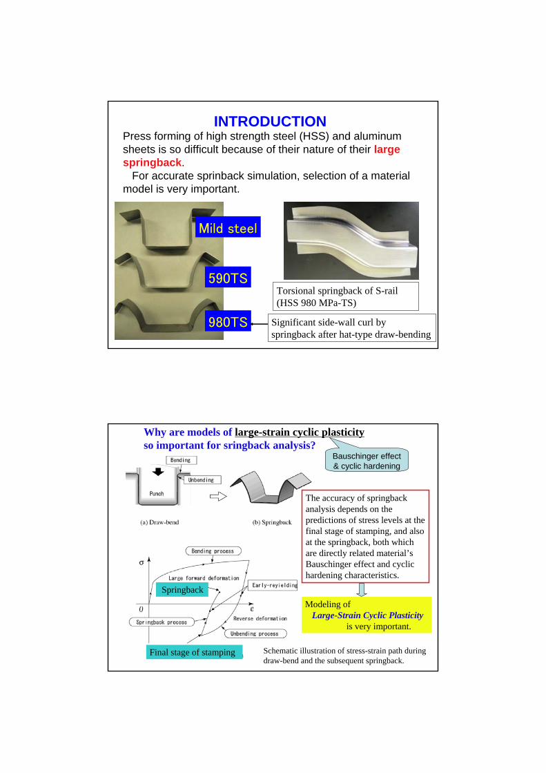
Significant side-wall curl by springback after hat-type draw-bending

Torsional springback of S-rail (HSS 980 MPa-TS)

980TS

Mild steel

590TS

INTRODUCTIONPress forming of high strength steel (HSS) and aluminum sheets is so difficult because of their nature of their large springback.

For accurate sprinback simulation, selection of a material model is very important.

Schematic illustration of stress-strain path during draw-bend and the subsequent springback.

Final stage of stamping

Springback

The accuracy of springbackanalysis depends on the predictions of stress levels at the final stage of stamping, and also at the springback, both which are directly related material’s Bauschinger effect and cyclic hardening characteristics.

Modeling of Large-Strain Cyclic Plasticity

is very important.

Why are models of large-strain cyclic plasticityso important for sringback analysis?

Bauschinger effect & cyclic hardening

Experimental observations of the Bauschinger effect

&Cyclic Plasticity Characteristics

Schematic illustrations of in-plane cyclic tension-compression tests of sheet metalsRef. F. Yoshida,T. Uemori, and K. Fujiwara,Int. J. Plasticity 18 (2002), pp.633-659.

* Other experimental techniques are by Wagoner (2004) and Kuwabara (2005).

In-Plane Cyclic Tension-Compression Tests of Sheet Metals

Cyclic Plasticity Characteristics

Transient Bauschinger effect and the permanent stress offset in reverse deformation

SPFC (high strength steel)

Isotropic hardening (IH) model

Permanent stress offset

Transient Bauschingereffect

Early re-yielding

Stress-strain responses of SPCC and SPCF (high-strength steel) under in-plane cyclic tension-compression (experimental data)

Experimental observations of cyclic strainingCyclic strain range dependency of cyclic hardening

Workhardening stagnation caused by the dissolution of dislocation cell walls and formation of new structures under reverse deformation

- ref. T. Hasegawa and T. Yakou, Mat. Sci. Eng. 20 (1975), pp.267-276

Effect of pre-strain on the subsequent cyclic behavior

Stress-strain responses of SPCC under in-plane cyclic tension-compression with various pre-strains (experimental data)

Non-workhardening under small-strain cycling after large pre-strain

SPCN590R (precipitation H)

SPCN590G(TRIP)

SPCN780G(TRIP)

SPCN980Y(DP)

The following material behavior should be modeled for sheet-metal forming simulation

Bauschinger effect & Cyclic plasticity• Early re-yielding, transient Bauschinger effect and

permanent stress offset in reverse deformation• Workhardening stagnation• Strain-range dependent cyclic workhardening

Anisotropy (r-value & flow stress directionality, biaxial flow stresses).

+

Yield functions: Hill (1948, 1990), Gotoh (1977), Barlat (1997, .., 2007), Vegter (2005), Banabic(2005), Yoshida (2011)

Models of Large-Strain Cyclic Plasticity(Framework of modeling)

With the assumption of small elastic strain and large plastic deformation, the rate of deformation D is decomposed as:

The constitutive equation of elasticity:

where

e p= +D D D

p= + ΩW W

: e= + =&οσ σ − Ωσ σ Ω C D

Continuum spin Plastic spin Spin of substructures

Objective rate of Cauchy stress Elasticity modulus

(2 / 3) :p pp ε= =&& D D

Modeling of Cyclic PlasticityInitial yield function

Subsequent yield function and the associated flow rule

( )0 0f Yφ= − =σ

：Cauchy stress Y：Yield strengthσ

Combined isotropic/kinematic hardening model

( ) ( ) 0,

p

f Y R

f

φ= − + =

∂= λ∂

&D

σ α

σ

−

backstress

Anisotropic yield function

Isotropic H

ijαY

Y R+ijσ

O

pijD

Several types Kinematic Hardening Laws(Evolution equation of backstress)

• Linear KH (Prager 1949)• A-F model (Armstrong-Frederick, 1966)• Mroz (1967)• Dafalias-Popov (1976)• Chaboche (1979, 1983)• Ohno-Wang (1993)• Teodosiu-Hu (1995)• Yoshida-Uemori (2002, 2003)

* are Large-Strain Cyclic Plasticity Model

Some of Kinematic Hardening Laws

• Linear KH (Prager 1949)

• A-F model (Armstrong-Frederick, 1966)

• Chaboche (1979, 1983)

• Yoshida-Uemori (2002, 2003)

2'3

pC=& &α ε

2' ' , ' '3

pi i i i iC γ ε= −∑ && &

Μ

ι=1

α = α α ε α

2' '3

pC γ ε= − && & &α ε α

( )a aCY

εα

∗ ∗∗

⎡ ⎤⎛ ⎞= − = −⎢ ⎥⎜ ⎟⎝ ⎠⎢ ⎥⎣ ⎦

o o o&α α β σ α α−

-400

-200

0

200

400

-0.1 -0.05 0 0.05 0.1 0.15 0.2 0.25

ExperimentIH+NLK+LK model

True strain ε

SPCC

Even by some complicated models, such as IH+AF-type NLK+LK model, cyclic hardening characteristics are so difficult to describe.

Constitutive Modeling of Large-strain Cyclic Plasticity

for Anisotropic Sheets

Yoshida-Uemori model

Yoshida, F and Uemori, T: Int. J. Plasticity, 18 (2002), 661Int. J. Mechanical Sicences, 45 (2003), 1687

Anisotropic Model of Large-Strain Cyclic PlasticityInitial yield function

Subsequent yield function and the associated flow rule

Bounding surface

( )0 0f Yφ= − =σ

( ) ( ) 0F B Rφ= − + =σ β−

：Cauchy stress Y：Yield strengthσ

Two surface model

( ) 0, p ff Yφ ∂= − = = λ

∂&σ α

σ− D

backstress

Anisotropic yield function

Kinematic H Isotropic H

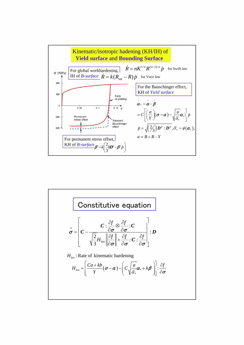
Kinematic/isotropic hadening (KH/IH) of Yield surface and Bounding Surface

For global workhardening, IH of B-surface ( )satR k R R p= −& &

For permanent stress offset, KH of B-surface 2' '

3pk b p⎛ ⎞= −⎜ ⎟

⎝ ⎠&Dβ β

o

For the Bauschinger effect, KH of Yield surface

( )

( ) ( )2 : , ,3p p

a aC pY

p

a B R Y

α

σ φ

∗

∗∗

∗ ∗

= −

⎡ ⎤⎛ ⎞= −⎢ ⎥⎜ ⎟⎝ ⎠⎣ ⎦

= =

= + −

o o o

&

&

α α β

σ α α

α

−

D D

1/ ( 1) /n n nR nK R p−=& & for Swift law

for Voce law

Constitutive equation

: ::

2 : :3

o

kin

f f

f f fH

⎡ ⎤∂ ∂⊗⎢ ⎥∂ ∂⎢ ⎥= −

⎢ ⎥∂ ∂ ∂+⎢ ⎥∂ ∂ ∂⎣ ⎦

σ σσ

σ σ σ

C CC D

C

( ) **

: Rate of kinematic hardening

:

kin

kin

H

Ca kb a fH C kY α

⎡ ⎤⎛ ⎞+ ∂= − − +⎢ ⎥⎜ ⎟⎜ ⎟ ∂⎢ ⎥⎝ ⎠⎣ ⎦

σ α α βσ

Schematic illustrations of the motion of: (a) the yield surface; and (b) the bounding surface under a uniaxial forward-reverse deformation.

Description of Workhardening Stagnation by assuming non-IH of bounding surface

Non-IH hardening of bounding surfaceWorkhardening stagnation

( ) ( )(1 )pfow k

bound satB R B R b e εσ β −= + + = + + −Explicit form!

Description of Workhardening Stagnation

by non-IH stress surface model

( )

( ) ( )1 3 :,

2hr r

μ

μ

′ ′ ′=

′ ′−= =

o

o

q q

q

β −

Γ β − βΓ

Schematic illustration of the non-IH surface defined in the stress space, when (a) non IH; and (b) IH takes place.

gσ

When

Otherwise 0R =& [non IH-hardening].

0R>&When r hΓ=&,when 0R =& ,

Kinematic motion and expansion of gσ

0r =&

0R =&( ', ', ) 0g rσ σ =q and ( ', ', ) : 0'

og rσ σ ββ

∂=

∂q

[hardening]0R>&

0 1h< <

0R >&

Example of stress-strain response under stress reversal and the definition of average

Young’s modulus Average Young’s modulus vsplastic prestrain

Plastic-strain dependent Young’s Modulus

F. Yoshida,T. Uemori, and K. Fujiwara,Int. J. Plasticity 18 (2002), pp.633-659.

Material Parameter Identification

• Automatic identification based on optimization technique

• M-Parameter identification tool: MatPara

CEM Inst Co. Ltd.

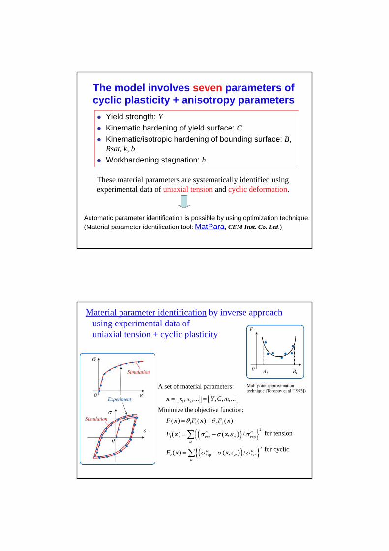
The model involves seven parameters of cyclic plasticity + anisotropy parameters

Yield strength: YKinematic hardening of yield surface: CKinematic/isotropic hardening of bounding surface: B, Rsat, k, bWorkhardening stagnation: h

These material parameters are systematically identified using experimental data of uniaxial tension and cyclic deformation.

Automatic parameter identification is possible by using optimization technique.(Material parameter identification tool: MatPara, CEM Inst. Co. Ltd.)

Material parameter identification by inverse approach using experimental data of uniaxial tension + cyclic plasticity

σ

ε

A set of material parameters:

Minimize the objective function:

for tension

for cyclic

1 2, ,... , , ,...x x Y C m= =⎢ ⎥ ⎢ ⎥⎣ ⎦ ⎣ ⎦x

( ){ }( ){ }

1 1 2 22

1 exp exp

2

2 exp exp

( ) ( ) ( )

( ) ( ) /

( ) ( ) /

F F F

F

F

α αα

α

α αα

α

θ θ

σ σ ε σ

σ σ ε σ

= +

= −

= −

∑

∑

x x x

x x,

x x,

Material parameter identification by inverse approach using experimental data of cyclic bending

Performance of the model

• Cyclic plasticity behavior• Non-proportional loading problem

Cyclic stress-strain responses under cyclic deformation calculated by the present model, together with the experimental results (Yoshida et al.) of high strength steel sheet (SPFC).

Strong Bauschinger effect appearing in 590 MPa HSS sheet

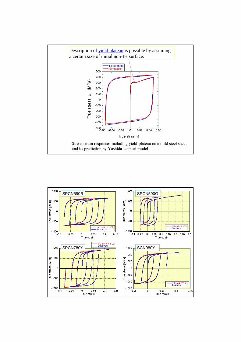
Cyclic stress-strain responses under cyclic deformation calculated by the present model, together with the experimental results (Yoshida et al.) of mild steel sheet (SPCC).

Y-U model can describe the Bauschinger effect, workhardeningstagnation, strain range and pre-strain dependent cyclic hardening.

Description of yield plateau is possible by assuming a certain size of initial non-IH surface.

SPCN590R

SCN980YSPCN780Y

SPCN590G

SCN980Y

HSS sheet (980 DP)(Y-U model + Hill 90 Yield function)

Aluminum sheet A5052(Y-U model + Barlat 2000 Yield function)

2 112

ε ε= −

1 2ε ε=

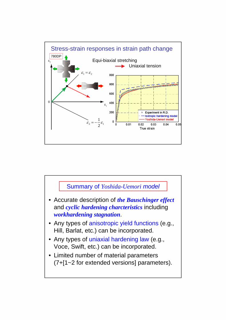
Stress-strain responses in strain path change

Equi-biaxial stretching Uniaxial tension

780DP

Summary of Yoshida-Uemori model

• Accurate description of the Bauschinger effectand cyclic hardening charcteristics including workhardening stagnation.

• Any types of anisotropic yield functions (e.g., Hill, Barlat, etc.) can be incorporated.

• Any types of uniaxial hardening law (e.g., Voce, Swift, etc.) can be incorporated.

• Limited number of material parameters (7+[1~2 for extended versions] parameters).