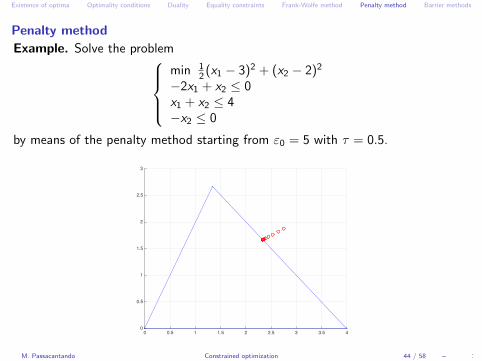
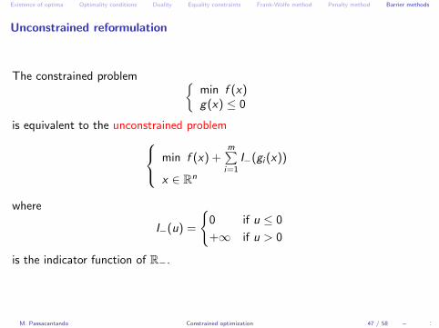
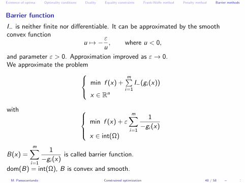
Existence of optima Optimality conditions Duality Equality constraints Frank-Wolfe method Penalty method Barrier methods Constrained optimization Mauro Passacantando Department of Computer Science, University of Pisa [email protected]Numerical Methods and Optimization Master in Computer Science – University of Pisa M. Passacantando Constrained optimization 1 / 58 –
Transcript
Existence of optima Optimality conditions Duality Equality constraints Frank-Wolfe method Penalty method Barrier methods
Numerical Methods and OptimizationMaster in Computer Science – University of Pisa
M. Passacantando Constrained optimization 1 / 58 –
Existence of optima Optimality conditions Duality Equality constraints Frank-Wolfe method Penalty method Barrier methods
Existence of global minima
A constrained optimization problem is defined as min f (x)g(x) ≤ 0h(x) = 0
where Ω = x ∈ D : g(x) ≤ 0, h(x) = 0 is the feasible region.
TheoremIf all the functions f , gi , hj are continuous, the domain D is closed and the feasibleregion Ω is bounded, then there exists a global minimum.
Example. min x1 + x2
x21 + x2
2 − 4 ≤ 0
admits a global minimum. Where?
M. Passacantando Constrained optimization 2 / 58 –
Existence of optima Optimality conditions Duality Equality constraints Frank-Wolfe method Penalty method Barrier methods
Existence of global optima
TheoremIf f is continuous, Ω is closed and there exists α ∈ R such that the α-sublevel set
x ∈ Ω : f (x) ≤ α
is nonempty and bounded, then there exists a global minimum.
Example. min ex1+x2
x1 − x2 ≤ 0−2x1 + x2 ≤ 0
Ω is closed and unbounded. The sublevel set x ∈ Ω : f (x) ≤ 2 is nonemptyand bounded, thus there exists a global minimum.
M. Passacantando Constrained optimization 3 / 58 –
Existence of optima Optimality conditions Duality Equality constraints Frank-Wolfe method Penalty method Barrier methods
Existence of global optima
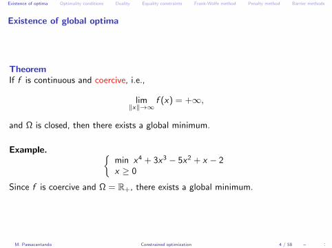
TheoremIf f is continuous and coercive, i.e.,
lim‖x‖→∞
f (x) = +∞,
and Ω is closed, then there exists a global minimum.
Example. min x4 + 3x3 − 5x2 + x − 2x ≥ 0
Since f is coercive and Ω = R+, there exists a global minimum.
M. Passacantando Constrained optimization 4 / 58 –
Existence of optima Optimality conditions Duality Equality constraints Frank-Wolfe method Penalty method Barrier methods
Existence and uniqueness of global optima
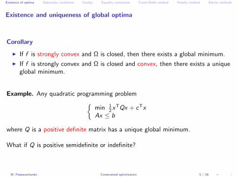
Corollary
I If f is strongly convex and Ω is closed, then there exists a global minimum.
I If f is strongly convex and Ω is closed and convex, then there exists a uniqueglobal minimum.
Example. Any quadratic programming problemmin 1
2xTQx + cTx
Ax ≤ b
where Q is a positive definite matrix has a unique global minimum.
What if Q is positive semidefinite or indefinite?
M. Passacantando Constrained optimization 5 / 58 –
Existence of optima Optimality conditions Duality Equality constraints Frank-Wolfe method Penalty method Barrier methods
Existence of global optima for quadratic programming problems
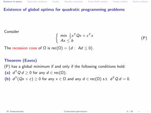
Consider min 1
2xTQx + cTx
Ax ≤ b(P)
The recession cone of Ω is rec(Ω) = d : Ad ≤ 0.
Theorem (Eaves)
(P) has a global minimum if and only if the following conditions hold:
(a) dTQ d ≥ 0 for any d ∈ rec(Ω);
(b) dT(Qx + c) ≥ 0 for any x ∈ Ω and any d ∈ rec(Ω) s.t. dTQ d = 0.
M. Passacantando Constrained optimization 6 / 58 –
Existence of optima Optimality conditions Duality Equality constraints Frank-Wolfe method Penalty method Barrier methods
Existence of global optima for quadratic programming problems
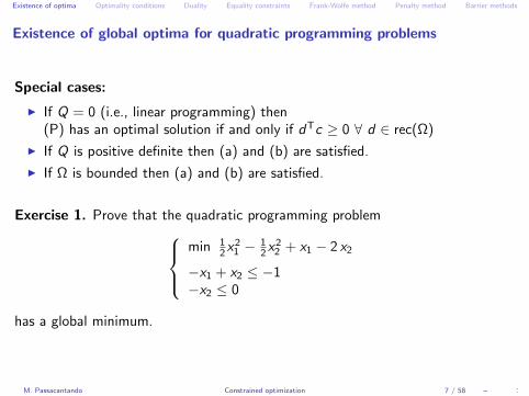
Special cases:
I If Q = 0 (i.e., linear programming) then(P) has an optimal solution if and only if dTc ≥ 0 ∀ d ∈ rec(Ω)
I If Q is positive definite then (a) and (b) are satisfied.
I If Ω is bounded then (a) and (b) are satisfied.
Exercise 1. Prove that the quadratic programming problemmin 1
2x21 − 1
2x22 + x1 − 2 x2
−x1 + x2 ≤ −1−x2 ≤ 0
has a global minimum.
M. Passacantando Constrained optimization 7 / 58 –
Existence of optima Optimality conditions Duality Equality constraints Frank-Wolfe method Penalty method Barrier methods
Constrained problems
Example. min x1 + x2
x21 + x2
2 − 4 ≤ 0
Ω = B(0, 2), global minimum is x∗ = (−√
2,−√
2), ∇f (x∗) = (1, 1).
Definition (Tangent cone)
TΩ(x) =
d ∈ Rn : ∃ zk ⊂ Ω, ∃ tk > 0, zk → x , tk → 0, lim
k→∞
zk − x
tk= d
Example (continued). What is TΩ(x∗)?
M. Passacantando Constrained optimization 8 / 58 –
Existence of optima Optimality conditions Duality Equality constraints Frank-Wolfe method Penalty method Barrier methods
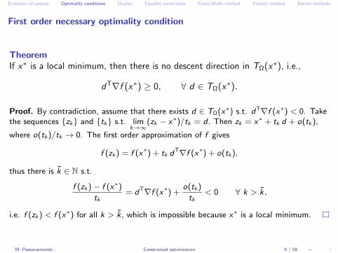
First order necessary optimality condition
TheoremIf x∗ is a local minimum, then there is no descent direction in TΩ(x∗), i.e.,
dT∇f (x∗) ≥ 0, ∀ d ∈ TΩ(x∗).
Proof. By contradiction, assume that there exists d ∈ TΩ(x∗) s.t. dT∇f (x∗) < 0. Takethe sequences zk and tk s.t. lim
k→∞(zk − x∗)/tk = d . Then zk = x∗ + tk d + o(tk),
where o(tk)/tk → 0. The first order approximation of f gives
f (zk) = f (x∗) + tk dT∇f (x∗) + o(tk),
thus there is k ∈ N s.t.
f (zk)− f (x∗)
tk= dT∇f (x∗) +
o(tk)
tk< 0 ∀ k > k,
i.e. f (zk) < f (x∗) for all k > k, which is impossible because x∗ is a local minimum.
M. Passacantando Constrained optimization 9 / 58 –
Existence of optima Optimality conditions Duality Equality constraints Frank-Wolfe method Penalty method Barrier methods
First order optimality condition for convex problems
TheoremIf Ω is convex, then Ω ⊆ TΩ(x) + x for any x ∈ Ω.
Optimality condition for constrained convex problems
If the optimization problem is convex, then x∗ is a global minimum if and only if
(y − x∗)T∇f (x∗) ≥ 0, ∀ y ∈ Ω.
Exercise 2. Prove the latter result.
M. Passacantando Constrained optimization 10 / 58 –
Existence of optima Optimality conditions Duality Equality constraints Frank-Wolfe method Penalty method Barrier methods
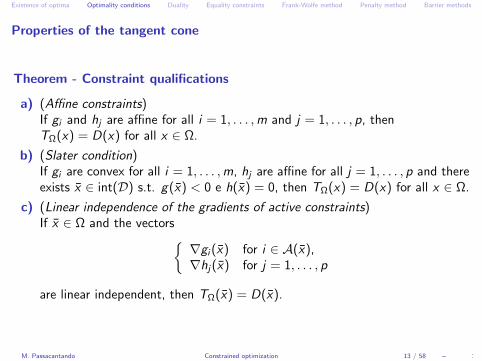
Properties of the tangent cone
TΩ(x) is related to geometric properties of Ω.
Which is the relation between TΩ(x) and constraints g , h defining Ω?
Example (continued). g(x) = x21 + x2
2 − 4, ∇g(x∗) = (−2√
2,−2√
2),
TΩ(x∗) = d ∈ R2 : dT∇g(x∗) ≤ 0
Definition (First-order feasible direction cone)
Given x ∈ Ω, A(x) = i : gi (x) = 0 denotes the set of inequality constraintswhich are active at x . The set
D(x) =
d ∈ Rn :
dT∇gi (x) ≤ 0 ∀ i ∈ A(x),dT∇hj(x) = 0 ∀ j = 1, . . . , p
is called the first-order feasible direction cone at point x .
M. Passacantando Constrained optimization 11 / 58 –
Existence of optima Optimality conditions Duality Equality constraints Frank-Wolfe method Penalty method Barrier methods
M. Passacantando Constrained optimization 12 / 58 –
Existence of optima Optimality conditions Duality Equality constraints Frank-Wolfe method Penalty method Barrier methods
Properties of the tangent cone
Theorem - Constraint qualifications
a) (Affine constraints)If gi and hj are affine for all i = 1, . . . ,m and j = 1, . . . , p, thenTΩ(x) = D(x) for all x ∈ Ω.
b) (Slater condition)If gi are convex for all i = 1, . . . ,m, hj are affine for all j = 1, . . . , p and thereexists x ∈ int(D) s.t. g(x) < 0 e h(x) = 0, then TΩ(x) = D(x) for all x ∈ Ω.
c) (Linear independence of the gradients of active constraints)If x ∈ Ω and the vectors
∇gi (x) for i ∈ A(x),∇hj(x) for j = 1, . . . , p
are linear independent, then TΩ(x) = D(x).
M. Passacantando Constrained optimization 13 / 58 –
Existence of optima Optimality conditions Duality Equality constraints Frank-Wolfe method Penalty method Barrier methods
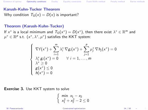
Karush-Kuhn-Tucker Theorem
Why condition TΩ(x) = D(x) is important?
Theorem (Karush-Kuhn-Tucker)
If x∗ is a local minimum and TΩ(x∗) = D(x∗), then there exist λ∗ ∈ Rm andµ∗ ∈ Rp s.t. (x∗, λ∗, µ∗) satisfies the KKT system:
∇f (x∗) +m∑i=1
λ∗i ∇gi (x∗) +
p∑j=1
µ∗j ∇hj(x∗) = 0
λ∗i gi (x∗) = 0 ∀ i = 1, . . . ,m
λ∗ ≥ 0g(x∗) ≤ 0h(x∗) = 0
Exercise 3. Use KKT system to solvemin x1 − x2
x21 + x2
2 − 2 ≤ 0
M. Passacantando Constrained optimization 14 / 58 –
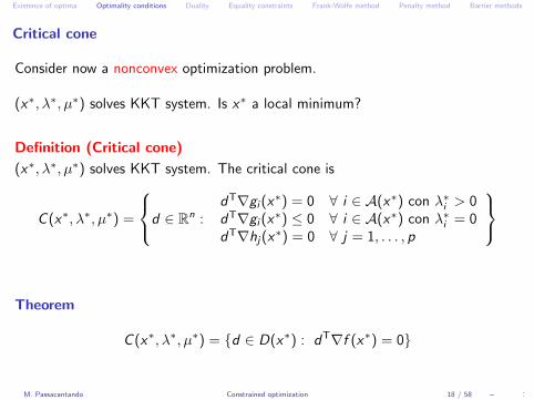
Existence of optima Optimality conditions Duality Equality constraints Frank-Wolfe method Penalty method Barrier methods
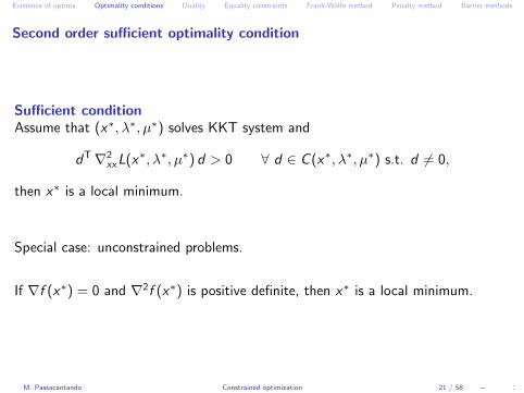
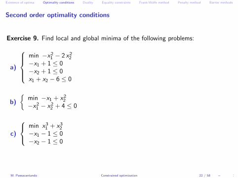
Karush-Kuhn-Tucker Theorem
Assumption TΩ(x∗) = D(x∗) is crucial.
Example. min x1 + x2
(x1 − 1)2 + (x2 − 1)2 − 1 ≤ 0x2 ≤ 0
x∗ = (1, 0) is the global minimum. TΩ(x∗) 6= D(x∗).
M. Passacantando Constrained optimization 31 / 58 –
Existence of optima Optimality conditions Duality Equality constraints Frank-Wolfe method Penalty method Barrier methods
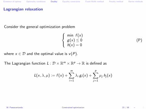
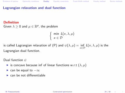
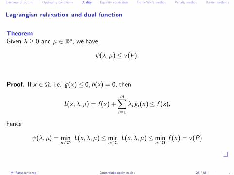
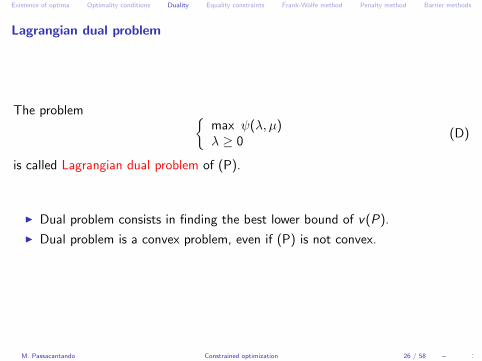
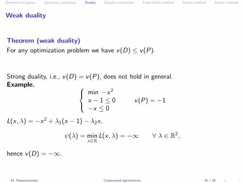
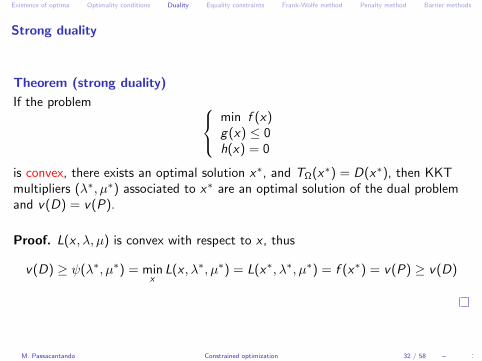
Strong duality
Theorem (strong duality)
If the problem min f (x)g(x) ≤ 0h(x) = 0
is convex, there exists an optimal solution x∗, and TΩ(x∗) = D(x∗), then KKTmultipliers (λ∗, µ∗) associated to x∗ are an optimal solution of the dual problemand v(D) = v(P).
Proof. L(x , λ, µ) is convex with respect to x , thus