Constraining models of postglacial rebound using space ...

Geophys. J. Int. (2010) doi: 10.1111/j.1365-246X.2010.04562.x

GJI

Geo

dyna

mic

san

dte

cton

ics

Constraining models of postglacial rebound using space geodesy:a detailed assessment of model ICE-5G (VM2) and its relatives

Donald F. Argus1 and W. Richard Peltier2

1Jet Propulsion Laboratory, California Institute of Technology, Pasadena, CA, 91109, USA. E-mail: [email protected] of Physics, University of Toronto, Toronto, ON, M5S 1A7, Canada

Accepted 2010 February 11. Received 2010 February 10; in original form 2009 August 27

S U M M A R YUsing global positioning system, very long baseline interferometry, satellite laser ranging andDoppler Orbitography and Radiopositioning Integrated by Satellite observations, includingthe Canadian Base Network and Fennoscandian BIFROST array, we constrain, in models ofpostglacial rebound, the thickness of the ice sheets as a function of position and time and theviscosity of the mantle as a function of depth. We test model ICE-5G VM2 T90 Rot, whichwell fits many hundred Holocene relative sea level histories in North America, Europe andworldwide. ICE-5G is the deglaciation history having more ice in western Canada than ICE-4G; VM2 is the mantle viscosity profile having a mean upper mantle viscosity of 0.5 × 1021 Pa sand a mean uppermost-lower mantle viscosity of 1.6 × 1021 Pa s; T90 is an elastic lithospherethickness of 90 km; and Rot designates that the model includes (rotational feedback) Earth’sresponse to the wander of the North Pole of Earth’s spin axis towards Canada at a speed of≈1◦ Myr−1.

The vertical observations in North America show that, relative to ICE-5G, the Laurentide icesheet at last glacial maximum (LGM) at ≈26 ka was (1) much thinner in southern Manitoba, (2)thinner near Yellowknife (Northwest Territories), (3) thicker in eastern and southern Quebecand (4) thicker along the northern British Columbia–Alberta border, or that ice was unloadedfrom these areas later (thicker) or earlier (thinner) than in ICE-5G. The data indicate thatthe western Laurentide ice sheet was intermediate in mass between ICE-5G and ICE-4G. Thevertical observations and GRACE gravity data together suggest that the western Laurentide icesheet was nearly as massive as that in ICE-5G but distributed more broadly across northwesternCanada.

VM2 poorly fits the horizontal observations in North America, predicting places alongthe margins of the Laurentide ice sheet to be moving laterally away from the ice centre at2 mm yr−1 in ICE-4G and 3 mm yr−1 in ICE-5G, in disagreement with the observation that theinterior of the North American Plate is deforming more slowly than 1 mm yr−1. SubstitutingVM5a T60 for VM2 T90, that is, introducing into the lithosphere at its base a layer with a highviscosity of 10 × 1021 Pa s, greatly improves the fit of the horizontal observations in NorthAmerica. ICE-4G VM5a T60 Rot predicts most of the North American Plate to be movinghorizontally more slowly than ≈1 mm yr−1, in agreement with the data.

ICE-5G VM5a T60 Rot well fits both the vertical and horizontal observations in Europe.The space geodetic data cannot distinguish between models with and without rotational

feedback, in the vertical because the velocity of Earth’ centre is uncertain, and in the horizontalbecause the areas of the plate interiors having geodetic sites is not large enough to detect thesmall differences in the predictions of rotational feedback going across the plate interiors.

Key words: Satellite geodesy; Global change from geodesy; Glaciology; Dynamics: gravityand tectonics; Kinematics of crustal and mantle deformation.

1 I N T RO D U C T I O N

Elevated beach terraces along the coastlines of Canada and Scandi-navia record Earth’s isostatic response to unloading of the ice sheets

since the last glacial maximum (LGM) at ≈26 ka (26 000 yr BP),and coral reefs in the tropics record the resulting rise of global sealevel. Relative sea level histories determined by radiocarbon datingof beach terraces (e.g. Peltier 2002a) and Uranium–Thorium dating

C© 2010 RAS 1Journal compilation C© 2010 RAS

Geophysical Journal International

2 D. F. Argus and W. R. Peltier

of coral reef deposits are the main observations constraining vis-coelastic models of postglacial rebound (Peltier 1994, 1996, 2004;Kaufmann & Lambeck 1997; Milne et al. 2001; Peltier & Fairbanks2006; Paulson et al. 2007; Sella et al. 2007). Such models accountfor both the transformation of the ice sheets into ocean water andthe gravitational response of the oceans to the resulting deformationof solid Earth. The models depend on three correlated parameters:the mass of the ice sheets as a function of position and time, theviscosity of the mantle as a function of depth, and the thickness ofthe elastic lithosphere.

Space geodesy is now providing an exciting means by which tofurther constrain such postglacial rebound models. First, estimatesof vertical site motion well constrain former ice sheet thickness inthe interiors of the continents (insofar as the timing of the unload-ing of the ice sheets is well constrained by glacial geomorphology),where the ice sheet thickness is unconstrained by relative sea levelhistories. Second, estimates of horizontal site motion newly con-strain the rheology of the lithosphere and mantle.

In this study, we evaluate postglacial rebound models with ob-servations from global positioning system (GPS), satellite laserranging (SLR), very long baseline interferometry (VLBI) andDoppler Orbitography and Radiopositioning Integrated by Satellite(DORIS), including data from the (CBN) Canadian Base Network(M. Craymer, National Resources Canada, electronic communica-tion, 2006) and the Fennoscandian BIFROST network (Johanssonet al. 2002). At the heart of the analysis in this study is distinguishingbetween postglacial rebound, plate motion and (rotational feedback)Earth’s response to the wander of the North Pole of Earth’s spin axistowards Canada at ≈1◦ Myr−1. An important element distinguish-ing this study from others is that we also estimate the velocity ofEarth’s centre, the reference relative to which vertical motions aredescribed, rather than assuming the velocity of Earth’s centre to bethat estimated using SLR observations of NASA’s LAser GEOdy-namics Satellite (LAGEOS).

2 M O D E L S O F P O S T G L A C I A LR E B O U N D A N D RO TAT I O NA LF E E D B A C K

We compare the space geodetic observations against elements ofthe models of Peltier (1994, 1996, 2004, 2007) and Peltier &Drummond (2008), but focus on the last two models. The mainbasis on which the models are constructed is a global data baseof many hundred relative sea level (RSL) histories (Peltier 2007,fig. 16). We know of no other global models of postglacial reboundthat are generally available to the international community. Peltier& Luthcke (2009) present a detailed analysis of Earth’s rotationalresponse to glacial isostatic adjustment, emphasizing the high qual-ity fit of the theory to both the non-tidal acceleration in the rate ofrotation and the speed and direction of the wander of the spin axis.

In this study, we evaluate the impact on the fit to the spacegeodetic observations of varying four elements of the postglacialrebound models: the ice sheet thickness as a function of position andtime, the viscosity of the mantle as a function of depth, the thicknessof the elastic lithosphere, and whether or not we include the effectof rotational feedback, which is dominated by Earth’s response tothe wander of the North Pole of the spin axis towards Canada at≈1◦ Myr−1 over the past 100 yr as observed by the InternationalLatitude Service. Earth also deforms in response to the non-tidalacceleration in Earth’s rate of rotation (Stephenson & Morrison1995), but this deformation is negligible relative to that generatedby polar wander.

2.1 Ice sheet models

We compare the space geodetic observations against two modelsof ice sheet thickness as a function of time, ICE-4G (Peltier 1994,1996, 2002b) and ICE-5G (Peltier 2004, 2007; Peltier & Drummond2008; Fig. 1). In this study, we compare against the version of ICE-4G in Peltier (2002b) and ICE-5G version 1.3a (Peltier 2007).

In North America the Laurentide ice sheet at LGM is about25 per cent more massive in ICE-5G than in ICE-4G (Fig. 1). Eastof Hudson Bay ice sheet thickness in the two models is nearly thesame. West of Hudson Bay there is in ICE-5G at LGM a 4000 mthick Keewatin ice dome, much thicker than the 2500 m thick icesheet there in ICE-4G. Furthermore in ICE-5G at LGM a 4000 mthick ice ridge extends from the Keewatin dome south through LakeWinnipeg [southern Manitoba], whereas in ICE-4G there is no suchridge and the ice is only 2500 m thick.

Peltier (2002a, 2004) greatly increased the thickness of the west-ern Laurentide ice sheet in ICE-4G to that in ICE-5G in order to fitearly VLBI and GPS estimates of uplift at Yellowknife (Argus et al.1999), to fit early estimates of the time rate of change of gravity atEarth’s surface observed using absolute gravimeters along a profilefrom Churchill (on Hudson Bay) through Manitoba and Minnesotainto Iowa (Lambert et al. 2001), and to increase total sea level risesince LGM by ≈12 m to 120 m to fit relative sea level observa-tions at coral reefs from the island of Barbados in the CaribbeanSea (Peltier & Fairbanks 2006, fig. 5). However, the GPS and VLBIresults that we present herein, which are based on a significantlylonger time-series than those in Argus et al. (1999), suggest that thewestern Laurentide ice sheet was less massive than that in ICE-5G.

In Europe the Fennoscandian ice sheet at LGM in ICE-5G isnearly identical to that in ICE-4G. The ice sheet in the Barents Seais also similar in the two models. The ice sheet in Novaya Zemlya,the Kara Sea, and northern continental Russia at LGM is eitherthinner in ICE-5G than in ICE-4G or absent in ICE-5G, satisfyingthe results of the (QUEEN) Quaternary Environment of the EurasianNorth project (Svendsen et al. 2004; Peltier 2004).

The Antarctica and Patgonian ice sheets in ICE-5G at LGMare identical to those in ICE-4G. In ICE-5G (version v1.3a) roughlyhalf of the excess Antarctic ice sheet at ≈26 ka disintegrates quicklyduring meltwater pulse 1b at 11 ka, as inferred on the basis of theRSL data at Barbados (Peltier & Fairbanks 2006) and radiocarbondating of the onset of marine sedimentation at many sites on theAntarctic shelf that constrain the retreat of the ice from the shelfbreak to be at ≈11 ka (Leventer et al. 2006). In ICE-4G the excessice disintegrates more gradually between 11 and 4 ka (Fig. 1).

2.2 Mantle viscosity models

We compare the space geodetic observations against three modelsof mantle viscosity as a function of depth, VM1 (Peltier 1994),VM2 (Peltier 1996, 2004) and VM5a (Peltier & Drummond 2008;Fig. 2). In all the models viscosity is laterally invariant. While theupper mantle above subducting slabs [e.g. Vancouver Island (Jameset al. 2009)] and hotspots [e.g. Iceland (Pagli et al. 2007)] may besignificantly less viscous than elsewhere, we maintain that through-out most of the mantle temperature and pressure increase along anadiabat (Turcotte & Schubert 1982), and therefore the mantle vis-cosity in areas near neither subduction zones, mid-ocean ridges, norhotspots is laterally nearly invariant. Because the Rayleigh numberof the mantle is high, heat transfer is mainly by convection and notconduction, and the horizontal distance over which mantle viscosity

C© 2010 RAS, GJI

Journal compilation C© 2010 RAS

Postglacial rebound from space geodesy 3

Figure 1. Mean sea level as a function of time for ICE-4G and ICE-5G (v1.3a) broken down into the ice sheet causing sea level rise (T, Total; N, NorthAmerica; E, Eurasia; A, Antarctica; G, Greenland). The mean sea level values are computed using the method of Peltier (2005) and Peltier & Fairbanks (2006),which does not use the ‘implicit ice’ method.

varies beneath spreading centres and subduction zones is believedto be small, on the order of the thickness of the thermal surfaceboundary layer (the lithosphere), as in the convection models ofSolheim & Peltier (1994). In any case we wish to test the hypothesisthat a mantle that is laterally invariant can fit all the observations.

VM1 is a two layer model in which the upper mantle and transitionzone have a viscosity of 1 × 1021 Pa s, and the lower mantle has aviscosity of twice that. The boundary between the transition zoneand lower mantle is at 660 km depth, the seismically observeddepth at which the phase transformation from spinel to a mixture ofperovskite and magnesiowustite occurs.

Figure 2. Mantle viscosity as a function of depth in VM1 (Peltier 1994),VM2 (Peltier 2006), VM5a (Peltier & Drummond 2008) and VM2–1(Paulson et al. 2007). In VM5a a thin layer of high viscosity (10 × 1021 Pa s)is between 60 and 100 km depth.

In VM2 the viscosity of the mantle varies in a detailed fashionas estimated by a formal Bayesian inversion of a subset of the RSLdata that depend only weakly on the deglaciation history. Frechetkernels (Peltier 2004, fig. 5) show the range of mantle depths overwhich different observations constrain the viscosity. RSL historiesfrom sites in Fennoscandia constrain the mean viscosity of the uppermantle and transition zone to be ≈0.5 × 1021 Pa s, about half that inVM1. In particular, VM2 fits the McConnell spectrum describingthe relaxation time of Fennoscandian rebound as a function of hor-izontal wave number, whereas VM1 does not (Peltier 2004, fig. 4).Given the upper mantle viscosity in VM2, RSL histories from sitesin Laurentia constrain the mean viscosity of the upper 500 km of thelower mantle to be ≈1.6 × 1021 Pa s. Two geophysical observables,the wander of Earth’s spin axis since 1900 (Gross & Vondrak 1999;Argus & Gross 2004) and the non-tidal acceleration of Earth’s rota-tion rate (Stephenson & Morrison 1995), constrain the viscosity ofthe remainder of the mantle to be ≈3.2 × 1021 Pa s (Peltier 2007,fig. 18).

VM5a differs from VM2 in two regards. First, VM5a is, be-neath the lithosphere, a three layer approximation of VM2. Second,whereas in VM2 the lithosphere is entirely elastic and 120 km thick(Peltier 1996) or 90 km thick (Peltier 2004), in VM5a the litho-sphere consists of an elastic layer 60 km thick above a highly viscous(10 × 1021 Pa s) layer 40 km thick.

Paulson et al. (2007) find that, given the ice sheet thickness inICE-5G plus or minus 20 per cent, VM2 is indeed consistent withRSL histories and GRACE gravity data in North America. Paulsonet al.’s (2007) study is an independent validation of Peltier’s (2004,2007, 2009) models, and rules out the hypothesis that the viscosityof the mantle increases by very much more across the 660 km depthhorizon than the factor of 3–4 in either VM2 or VM5a.

2.3 Elastic lithosphere thickness

We compare the space geodetic observations against two values ofthe thickness of the elastic lithosphere, 90 km (Peltier 2007) and60 km (Peltier & Drummond 2008). Decreasing the thickness of theelastic lithosphere increases the gradient in vertical motion alongthe margins of the former ice sheets (Peltier 1986).

C© 2010 RAS, GJI



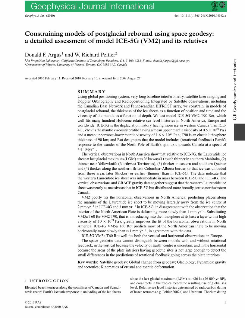
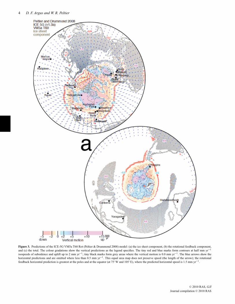
Figure 3. Predictions of the ICE-5G VM5a T60 Rot (Peltier & Drummond 2008) model: (a) the ice sheet component, (b) the rotational feedback component,and (c) the total. The colour gradations show the vertical predictions as the legend specifies. The tiny red and blue marks form contours at half mm yr−1

isospeeds of subsidence and uplift up to 2 mm yr−1; tiny black marks form grey areas where the vertical motion is 0.0 mm yr−1. The blue arrows show thehorizontal predictions and are omitted where less than 0.5 mm yr−1. This equal area map does not preserve speed (the length of the arrow); the rotationalfeedback horizontal prediction is greatest at the poles and at the equator (at 75◦W and 105◦E), where the predicted horizontal speed is 1.5 mm yr−1.

C© 2010 RAS, GJI



2.4 Effect of rotational feedback

The models of Peltier (2004), Peltier (2007) and Peltier &Drummond (2008) consist of two components, an ice sheet com-ponent and a rotational feedback component (Fig. 3). The ice sheetcomponent consists of solid Earth’s viscoelastic response to unload-ing of the late Pleistocene ice sheets and the resulting loading ofthe ocean basins by water (ice and water surface loads). The ro-

tational feedback component consists of solid Earth’s viscoelasticresponse to secular polar wander in the postglacial rebound model(centrifugal body force), which ultimately also results from ice sheetloss. The predictions of these models of the present-day wander ofthe North Pole of Earth’s spin axis do not differ greatly (Peltier2007, Tables 1 and 2) from the observed mean velocity of 0.0035arcsec yr−1 along the 79◦W meridian (Gross & Vondrak 1999;Argus & Gross 2004; see Appendix A). The models of Peltier (1994,

Figure 3. (Continued.)

C© 2010 RAS, GJI




1996) neglect the effect of rotational feedback. Herein we designatewhether or not a postglacial rebound model includes rotational feed-back using ‘Rot’ or ‘No Rot’. Rotational feedback generates, in thevertical, a degree-2 order-1 pattern with maximum uplift and subsi-dence of 1.5 mm yr−1 (in ICE-5G VM5a T60 Rot) at four locationsalong the 75◦W–105◦E great circle, two at 45◦N and two at 45◦S.

Rotational feedback also causes places to be moving horizontallyaway from the areas of subsidence and towards the areas of uplift.This sense is opposite that for postglacial rebound because Earth’sresponse to a body force (rotational feedback) differs from that to asurface force (postglacial rebound). Horizontal speed is a maximumof 1.5 mm yr−1 (in ICE-5G VM5a T60) at four locations along the

C© 2010 RAS, GJI



Table 1. Space geodetic site velocity solutions.

Horizontal Vertical

Time Dist Sigma Dist Sigma TimeTechnique N (yr) (mm) (mm yr−1) (mm) (mm yr−1) Period Scientist [Institution]

GPS 319 6 (14) 4.5 0.7 (0.3) 10 1.6 (0.7) 1991–2007 Michael B. Heflin [Jet Propulsion Laboratory]VLBI 32 11 (17) 6 0.7 (0.4) 13 1.3 (0.8) 1979–2000 Chopo Ma [Goddard Space Flight Center]SLR 20 14 (18) 11 1.0 (0.7) 23 1.8 (1.3) 1976–2000 Richard J. Eanes [Center for Space Research]DORI 38 10 (13) 19 1.9 (1.5) 31 3.1 (2.4) 1993–2006 Pascal Willis [Institut Geographique National]BIF 53 8 (8) 4.5 0.9 (0.6) 10 1.5 (1.3) 1996–2004 Lidberg et al. 2007 [Onsala Space Observatory]CBN 157 10 (11) 4.5 0.7 (0.6) 10 2.6 (2.0) 1994–2006 Michael Craymer [National Resources Canada]

Notes: N , number of sites; Time, median effective time period of observation; Dist, distance used to compute the systematic error in site velocity (as describedin the text); Sigma, median standard error in velocity component. Values in parentheses are for the space technique’s 10 tightest constrained site velocities.The velocity sigmas that we infer are comparable to those Williams et al. (2004) estimate using maximum likelihood estimation. Williams et al. (2004)estimate that, in two global sets of position time-series, flicker noise to be 5–11 mm in the horizontal and 20 to 23 mm yr−1 in the vertical. Assuming flickernoise to be the main error source, and using eq. (32) of Bos et al. (2008), we find these to suggest systematic distance in the horizontal of 2–4 mm, and in thevertical of 7–8 mm, a little smaller than the 4.5 and 10 mm that we find. We and Williams et al. (2004) agree that the velocity sigmas are roughly 5–25 timesgreater than that inferred from linear propagation of position estimates.

75◦W–105◦E meridian, two along the equator and two at the Northand South Poles.

In ICE-4G VM5a T60 Rot rotational feedback creates a nearlyidentical pattern but speeds are about one-third smaller (because thetotal ice mass in ICE-4G is less than that in ICE-5G), with maximumuplift and subsidence of 1.1 mm yr−1 and maximum horizontalspeed of 1.0 mm yr−1. In ICE-5G VM2 T90 Rot maximum upliftand subsidence are 1.8 mm yr−1 and maximum horizontal speed is1.2 mm yr−1.

RSL histories near the areas in which the degree-2 order-1 patternof uplift and subsidence is greatest show the effect of rotationalfeedback to be close to that predicted by ICE-5G VM2 T90 Rot:east Patagonia and southern Japan (Ryukyu islands) rose up to≈12 m over the past 8 kyr (a rate of 1.5 mm yr−1), and southernAustralia subsided up to ≈6 m since 8 ka (a rate of 0.8 mm yr−1)(Peltier 2007, figs 21–25). Because these RSL data require the effectof rotational feedback to be large, we focus herein on comparisonsof the space geodetic observations with models that include theeffect of rotational feedback.

Mitrovica et al. (2005) find Earth’s vertical response to rota-tional feedback to have maximum uplift and subsidence of just≈0.25 mm yr−1, about six times less than predicted by the modelsof Peltier. However, Peltier & Luthcke (2009) show the formulationand prediction of Mitrovica et al. (2005) to be incorrect.

3 DATA

We invert six site velocity solutions from six institutions (Table 1).Four of the solutions are global. Twenty-one years of VLBI obser-vations and 24 yr of SLR observation [more than the 13 yr of SLRobservation in ITRF2005; Altamimi et al. 2007) tightly constrainvelocities in places, contributing towards determining Earth’s ref-erence frame. Sixteen years of global GPS observations provide asuperior geographic distribution to that of VLBI and SLR. Thir-teen years of global DORIS observations provide estimates of sitevelocity that are not as tightly constrained as for the other threetechniques. We completely describe this set of four global velocitysolutions in Argus et al. (2010, appendix B).

Two of the velocity solutions are regional. Campaign GPS ob-servations of the Canadian Base Network (CBN), with roughly 3–5observations per site, and with 7–11 yr of data, are in the area be-neath the former Laurentide ice sheet. Permanent GPS observations

of the BIFROST network provide information constraining Earth’sresponse to the former Fennoscandian ice sheet.

The GPS velocity solution that we invert in this study differs fromthat in GEODVEL (Argus et al. 2010) in that we add 150 GPS siteson the interior of the North American Plate in the Continually Oper-ating Reference Stations (CORS) and Forecast Systems Laboratory(FSL) networks. In this study, we determine model GEODVEL1busing means identical to that in GEODVEL except that we alsoinvert these additional data.

4 M E T H O D S

In this study we follow the methods of Argus et al. (1999, 2010)and Argus (2007).

4.1 Sites, places, plate interiors and glacial isostaticadjustment

4.1.1 Sites

In general we define a site to correspond to a velocity providedto us by an analysis institution. A VLBI site consists of 1–3 radiotelescopes less than 1000 m apart, an SLR site consists of 1–7 laserranging stations less than 1000 m apart, and a DORIS site consistsof 1–3 beacons less than 1000 m apart. [see Argus et al. (2010,appendix B) for three places at which we assume sites more than1000 m apart to comprise a place.]

We define a GPS site more narrowly than for VLBI and SLRbecause we wish to carefully evaluate GPS estimates of site velocity,which are subject to uncertainty due to antenna substitutions. Wedefine a GPS site to be an Antenna Reference Point (ARP); eachGPS site has a unique four-letter abbreviation in the InternationalGNSS Service (IGS). Thus we take GPS ARP’s meters or tens ofmeters apart to be distinct sites. (This differs from the definition ofa DOMES number, which groups ARP’s near each other into a site.)In general we estimate an offset for a logged antenna substitution ifthe offset appears to be more than ≈10 mm in the vertical or morethan ≈5 mm in the horizontal. If there is no logged antenna offset,we estimate a logged antenna substitution if the offset appears tobe more than ≈12 mm in the vertical or more than ≈6 mm in thehorizontal.

C© 2010 RAS, GJI



Table 2. Number of sites and places in (a) category rigid, (b) category glacial isostatic adjustmentand (c) category omit.

VLBI SLR GPS DORIS CBN BIFR Plate Sites Places

(a) Category rigid

1 7 5 Antarctica 13 103 Arabia 3 3

3 2 15 4 Australia 24 135 9 56 2 9 Eurasia 81 47

4 1 India 5 41 4 2 Nazca 7 3

11 4 145 3 6 N. America 169 1461 6 5 Nubia 12 9

5 2 9 6 Pacific 22 151 7 3 S. America 11 6

3 2 Somalia 5 3

26 19 259 33 6 9 Total 352 259

(b) Category glacial isostatic adjustment

1 3 1 Antarctica 5 21 9 1 44 Eurasia 55 432 23 2 151 N. America 178 1551 1 1 Macdonald 3 1

5 1 36 4 151 44 Total 241 201

(c) Category omit

1 Australia 1 11 3 1 Eurasia 5 2

19 N. America 19 191 Nubia 1 1

1 24 1 Total 26 23

Notes: A place in Category rigid is defined to consist of between 1 and 8 sites less than 30 km apart.A site or place in Category Rigid is on a plate interior, is not beneath or along the margin of a latePleistocene ice sheet, and is used to estimate the angular velocity of a plate in GEODVEL1b. A siteor place in Category Glacial Isostatic Adjusment is on a plate interior, has significant glacialisostatic adjustment (either uplift faster than 2.5 mm yr−1 or horizontal motions faster than0.5 mm yr−1), and is not used to estimate the angular velocity of a plate in GEODVEL1b. We usethe postglacial rebound model of Peltier [1996, ICE4G VM2 T90 No Rot] to evaluate whether aplace is rising faster than 2 mm yr−1. We use the model of Peltier [1994, ICE4G VM1 T60 No Rot]to evaluate whether a place is moving horizontally faster than 0.5 mm yr−1. We use the models ofPeltier (1996) and Peltier (1994) because they were the models that best fit, respectively, thehorizontal and vertical geodetic observations when we determined GEODVEL [Argus et al. 2010].These criteria result in places beneath or along the margins of the late Pleistocene ice sheets beingassigned to Cateogory GIA. We assign Macdonald Observatory [Texas], which is not on the NorthAmerican interior and is moving insignificantly in glacial isostatic adjustment, to Category GIAand estimate the velocity of Macdonald relative to the North American Plate interior because wewish to take advantage of the velocity tie between the SLR, GPS, and VLBI sites, all of which havea long history of observation. We omit places in Category Omit for the several reasons we state inthe Notes of Table S1c.

4.1.2 Places

We next assign sites to places, taking a place to consist of one toeight sites less than 30 km apart. We assume sites at a place to moveat the same velocity. In this way, we evaluate the relative accuracyof the four techniques. We can more readily interpret the velocityof a place, which is the weighted mean of the velocities of nearbysites. This weighted mean also tends to average away local biasesdue to ground instability and water management of aquifers.

4.1.3 Plate interiors and glacial isostatic adjustment

We assign places to plate interiors following the criteria of Argus &Gordon (1996), and following Argus et al. (1999, 2010). Places on

plate interiors are not in the belts of large and medium earthquakes,active major faults, and high topographic relief generated by activedeformation. A place on a plate interior is far enough from anyknown fault that the interseismic strain that is accumulating causesthe place to be moving relative to the plate interior more slowly than1 mm yr−1.

We next assign places to one of four categories:Category Rigid (Table S1c) consists of places on plate interiors

neither beneath nor along the margins of the former Laurentide icesheet.

Category GIA (Table S1b) consists of places on plate interi-ors either beneath or along the margins of the former Laurentideice sheets. Places in Category GIA have either uplift greater than2 mm yr−1 in the model of Peltier (1996, ICE4G VM2 T120 No Rot)

C© 2010 RAS, GJI



Figure 4. Velocities between definitions of Earth’s centre differently specifying the translational velocities of the GPS networks. (CM) centre of mass of Earth,oceans and atmosphere, (CE) centre of mass of solid Earth. In GEODVEL1b, we assume that, besides plate motion, the parts of the plate interiors not nearthe late Pleistocene ice sheets are not moving horizontally relative to CE. GEODVEL1b is nearly identical to GEODVEL (unlabeled dash black 95 per centconfidence limits) (Argus et al. 2009). CE Kogan 2008 is the velocity of CE that Kogan & Steblov (2008) estimate in a manner identical to that in GEODVEL1b.In ICE-5G VM5a T60 Rot, ICE-4G VM5a T60 Rot and ICE-4G VM5a T60 No Rot, we assume that the plate interiors are moving vertically and horizontallyrelative to CE as predicted by the postglacial rebound model. CM CSR (unlabeled maroon pentagon very near GEODVEL1b) is the velocity of CM determinedby the Center for Space Research in CSR00L01, the SLR velocity model that we invert. We place the ITRF and our estimates of the velocity of Earth’s centre onthe same plot by estimating the translational velocity and rotational velocity between the ITRF2000 (Altamimi et al. 2002) site velocities and the GEODVEL1bplace velocities.

or horizontal movement greater than 0.5 mm yr+ in the modelof Peltier (1994, ICE-4G VM1 T120 No Rot; see Notes ofTable 2b).

Category Omit (Table S1c) consists of 23 places on plate interiorsthat we do not use to constrain the postglacial rebound models forseveral reasons (see Notes of Table S1c).

Category Boundary consists of places in the deformation zonesbetween the plate interiors. We omit places in Category Boundary.

4.2 Inversion

If we were to evaluate the postglacial rebound models in straight-forward fashion, we would invert the velocity estimates of sites inCategory Rigid and Category GIA using the following relationshipbetween data, parameters, and postglacial rebound predictions:

vit − wgia = (ωa + Rt) × ri + Tt, (1)

where all quantities are 3-D vectors vit (a datum) is the velocityof site i estimated using space technique t, wgia is postglacial re-bound model prediction of the velocity of site i, ωa (a parameter)is the angular velocity of the plate the site is on, Rt (a parameter)is the angular velocity of the reference frame of the space tech-nique of the site, Tt (a parameter) is the translational velocity of thereference frame of the space technique of the site (which is thenegative of the velocity of CE relative to the site network ofthe technique), and ri (a constant) is the vector from Earth’s centreto the site.

However in this study we invert the velocity estimates in a slightlymore sophisticated manner using the following relationship

vit − wgia = (ωa + Rt) × ri + Tt + ub, (2)

where the vector ub (a parameter) is the velocity of place b. We varythe parameters that we estimate in three ways (following table 2 ofArgus et al. 1999 and table 5 of Argus et al. 2010).

To evaluate the postglacial rebound models, we set to zero the(ub’s) velocities of places in Category Rigid and Category GIA; thevelocity of a site in Category Rigid or Category GIA constrains

the (ωa) angular velocity of the plate it is on. We estimate the (ub’s)velocities of places in Category Omit, but do not assign places inCategory Omit to a plate. These inversions yield estimates of thevelocity of Earth’s centre (Fig. 4, PGR models) and is the basisof Figs 5–12 and S1–S5, excepting the figures stated in the nextparagraph.

To determine GEODVEL1b, we set to zero the horizontal com-ponents of the (ub’s) velocities of places in Category Rigid; thevelocity of a site in Category Rigid constrains the (ωa) angular ve-locity of the plate it is on. We estimate the (ub’s) velocities of placesin Category GIA and Category Omit, but do not assign places inCategory GIA or Category Omit to a plate. Assuming the velocityof 2 or more sites at a place to be equal constrains the translationvelocity and rotation velocity between the reference frames of theinput velocity solutions. This inversion yields an estimate of thevelocity of Earth’s centre (Fig. 4, GEODVEL1b) and estimates ofplace velocity that do not depend on a postglacial rebound model(Figs 6a, 8, 10, 11a, 13, S1 and Table S1).

We tie CBN sites to the GPS, VLBI and DORIS networks at 21places. We tie the BIFROST velocity sites to the GPS, VLBI andDORIS networks at 16 places. In the inversion we treat correlationsbetween all components of site velocity. But the point positioningmethod used for GPS and DORIS yields correlations of zero; andfor VLBI and SLR the random errors embedded in the correlationstend to be less than the systematic error that we add to obtain ourrealistic error budget.

4.3 Error budget

We formulate a realistic error budget following the method ofArgus & Gordon (1996), Argus (2007) and Argus et al. (2010).We take the true standard error in a site velocity component to bethe root sum square of a random error and a systematic error. Therandom error comes from the dispersion of positions about a con-stant velocity (for VLBI and SLR) or about a constant velocity anda sinusoid having a period of 1 yr (for GPS and DORIS). We com-pute the systematic error to be a distance (in mm) as we describe

C© 2010 RAS, GJI



Figure 5. Fits of models of postglacial rebound and rotational feedback to the vertical and horizontal observations, broken down by plate. Values of chi-squareare given. For each model we estimate the angular velocities of the plates and the velocity of Earth’s centre minimizing the misfit between the model anddata.

next and specify in Table 1, divided by the effective time periodof observation (in yr). The effective time period of observation of asite with an offset is the root sum square of the time period beforeand time period after the offset. For each of the four global tech-niques we determine the vertical distance just large enough to make

the estimates of vertical rate consistent among the four techniques;and the horizontal distance just large enough to make the esti-mates of horizontal velocity consistent among the four techniquesand consistent with the parts of the plate interiors not near the icesheets being rigid (as in GEODVEL1b). In sum we make the eight

C© 2010 RAS, GJI



Figure 6. Observed horizontal velocities relative to the North American Plate in the reference frame minimizing differences with (a) a model in which[GEODVEL1b] the parts of the plate interiors not near the late Pleistocene ice sheets are not deforming laterally, (b) ICE-4G VM2 T90 Rot and (c) ICE-4GVM5a T60 Rot. In (b) and (c) red arrows show predicted velocities and are omittted where less than 0.5 mm yr−1. Black arrows show well-constrainedobserved velocities; grey arrows show poorly constrained observed velocities. Error ellipses are 95 per cent confidence limits and are filled gold for the tightestconstrained velocities (semi major axis less than 0.5 mm yr−1), filled yellow for velocities either constrained medium well (semi major axis greater than0.5 mm yr−1 and less than 0.8 mm yr−1) or in the Canadian Arctic or in Greenland, and are omitted for poorly constrained velocities (semi major axis greaterthan 0.8 mm yr−1) elsewhere. In the horizontal illustrations (Figs 6, 11, S2 and S5) we first invert the data to estimate the best fitting parameters, next setthe translational and rotational velocities of the four techniques and the angular velocities of the plates to their best fitting values and invert the data for thevelocities of places on plates, then take the observed horizontal velocity to be the sum of the horizontal postglacial rebound prediction (wgia) of the placeand the horizontal velocity (horizontal components of ub) estimated in the second inversion. See Fig. S2 for the horizontal velocities of four other postglacialrebound models.

distances just large enough to make the normalized sample standarddeviations of the eight data subsets equal to one (see for example,table 4 of Argus et al. 1999). We assume the error budget for thecampaign GPS CBN and permanent GPS BIFROST networks to be

identical to that for the global permanent GPS network. The veloc-ity sigmas we infer are roughly comparable to those Williams et al.(2004) estimate using maximum likelihood estimation (see Notesof Table 1).

C© 2010 RAS, GJI




5 R E S U LT S

5.1 Velocity of Earth’s centre

Earth’s centre is fundamental to the study of postglacial reboundbecause it is the point relative to which site motions are estimated(Argus 1996; Heki 1996). That is, estimates of the rate of verticalmotion of a site depend entirely on the velocity of Earth’s centre(Argus et al. 1999; Argus 2007).

The velocity of (CM) the mass centre of Earth, oceans, and atmo-sphere differs between ITRF2000 and ITRF2005 by 1.8 mm yr−1

along Z (Fig. 4). This suggests that the velocity of CM is not con-

strained very tightly by SLR observations of satellite LAGEOS(Argus 2007).

The velocity of (CE) the mass centre of solid Earth determinedassuming (GEODVEL1b) that the parts of the plates not near the icesheets are not moving relative to CE lies along Z ≈ 1/3 of the wayfrom ITRF2000 to ITRF2005. The velocity of CE in GEODVEL1bis nearly identical to that in GEODVEL and to that determinedusing identical means by Argus (2007). But the velocity of CEalong Z in GEODVEL1b differs significantly by ≈1 mm yr−1 fromthe velocity of CE that Kogan & Steblov (2008) estimate. Argus(2007) and Argus et al. (2010, Appendix A) maintain that the speedbetween CE and CM is less than 0.2 mm yr−1.

C© 2010 RAS, GJI




The velocity of CE determined assuming that the plate interiorsare moving as predicted by ICE-4G VM5a T60 Rot lies along Zhalfway from ITRF2000 to ITRF2005. Along Y the velocity of CEin ICE-4G VM5a T60 Rot is nearer the velocity of CM in ITRF2005than is the velocity of CE in ICE-5G VM5a T60 Rot.

In this study, we quote estimates of uplift and subsidence relativeto the velocity of CE in GEODVEL1b because this definition doesnot depend on a specific postglacial rebound model.

5.2 Summary of fits of postglacial rebound models

We next describe the main results of this study (Fig. 5, Table 3).We describe misfit reductions in terms of the normalized sample

standard deviation (nssd), which is the square root of reduced chi-square). An nssd of 1.5 indicates that either the model fits the data50 per cent worse than a perfect model, or that the data errors are33 per cent too small. An nssd of 1 suggests that both the model fitsthe data well and that the data errors are realistic.

Substituting mantle and lithosphere profile VM5a T60 for VM2T90 significantly reduces horizontal misfits in North America. Thenssd decreases by a highly significant 130 per cent given ICE-5GRot, and by a highly significant 70 per cent given ICE-4G Rot(Fig. 5, Table 3). The probability p of the misfit falling this muchby chance is miniscule, 6.1 × 10−11 given ICE-4G Rot.

Substituting deglaciation history ICE-4G for ICE-5G reducesvertical misfits in North America by a significant (p = 0.00096)

C© 2010 RAS, GJI



Figure 7. Residuals of the observed vertical rates of sites on the North American Plate interior relative to the predictions of models (a) ICE-5G VM5a T60Rot and (b) ICE-4G VM5a T60 Rot. Green bars show positive residuals, orange bars negative residuals; Residual speeds are given in mm yr−1; Error barsare 95 per cent confidence limits; ‘X’s are the predictions of uplift or subsidence in the postglacial rebound model. L–L′ and M–M′ show the location of theprofiles in Fig. 8. The colour gradations show, as the legend specifies, the predictions of the postglacial rebound model. In Fig. 7(a) the large blue and redellipses show areas of significant misfit as stated in the text. The ice domes (‘D’s), ice saddles (‘S’s), and ice divide (thick magenta line) during last glacialmaximum are from Dyke & Prest (1987, supplemental fig. 2). In the vertical illustrations (Figs 7–10, S3 and S4) we plot the vertical weighted residuals of thesites at a place. See Fig. S2 for the residuals of four other postglacial rebound models.

42 per cent (given VM5a T60 Rot). This substitution furthermorereduces horizontal misfits in North America by 26 per cent, a re-duction that is insignificant (p = 0.070), but close to the p = 0.05threshold for being ‘significant’.

Substituting deglaciation history ICE-5G for ICE-4G reducesvertical misfits in Eurasia by 33 per cent (given VM5a T60 Rot). Thismisfit reduction is insignificant (p = 0.077), but again marginallyso.

C© 2010 RAS, GJI




Substituting ‘No Rot’ for ‘Rot’ changes misfits of all the databy less than 1 per cent. Substituting ‘No Rot’ for ‘Rot’ increasesvertical misfits by an insignificant 4 per cent and reduces horizontalmisfits by an insignificant 2 per cent (given ICE-4G VM5a T60).

Substituting mantle and lithosphere profile VM1 T90 for VM5aT60 reduces horizontal misfits by an insignificant (p = 0.21)6 per cent (given ICE-4G Rot). But VM1 T90 poorly fits the

McConnell spectrum describing the relaxation time of Fennoscan-dian rebound as a function of horizontal wave number (Peltier 2004,fig. 4). Given that pressure and temperature in the mantle increasealong an adiabat except near hotspots and subduction zones, weseek a global model of postglacial rebound having a mantle viscos-ity fitting all RSL and space geodetic observations from the cratons.VM1 and VM2 do not; VM5a may.

C© 2010 RAS, GJI



Figure 8. Observed vertical rates of motion of places as a function of angular distance along profile L–L′ and profile M–M′ (Fig. 7). Blue circles show upliftand red circles subsidence of VLBI, SLR and permanent GPS sites; open circles show campaign GPS sites of the Canadian Base Network; Error bars are95 per cent confidence limits. In the vertical profiles (Figs 8 and 10) the observed velocity is the estimated vertical component of ub in the GEODVEL1binversion.

5.3 Horizontal North America

In the reference frame [GEODVEL1b] minimizing the horizon-tal deformation of the parts of the plate interiors not near the icesheets, the North American Plate interior appears to be nearly rigidexcept for places near the margins of the former Laurentide icesheet (Fig. 6a). The weighted root mean square residual speed ofplaces not near the Laurentide ice sheet is 0.9 mm yr−1. [The 150FSL and CORS sites increase the dispersion from 0.6 mm yr−1 (inGEODVEL, Argus et al. 2010)]. Three places near the Laurentideice sheet have very significant (probability less than 0.01) velocitiesrelative to the North American Plate. Algonquin Park is movingsouth at 0.8 ± 0.5 mm yr−1, Yellowknife is moving south at 1.2 ±0.6 mm yr−1, and Thule (along the east coast of Greenland) is mov-ing southwest at 2.7 ± 1.2 mm yr−1 (Table S1b). (In this study,95 per cent confidence limits follow the ‘±’.)

VM2 T90 poorly fits the horizontal observations. ICE-5G pre-dicts the margins of the late Pleistocene Laurentide ice sheet tobe moving laterally away from the ice sheet at roughly 3 mm yr−1

(Fig. S2a), and ICE-4G predicts the margins to be moving laterallyaway from the ice centre at ≈2 mm yr−1 (Fig. 6b). These predictionsdisagree greatly with the horizontal observations, which show theNorth American Plate interior to be deforming very slowly if atall. In the VM2 T90 inversions, the velocity of the North AmericanPlate adjusts to fit the horizontal estimates of places where theyare constrained tightest in eastern North America (at Greenbelt,Algonquin Park, and Westford], but that plate velocity poorly fitsthe horizontal estimates elsewhere [at Yellowknife, North Liberty,and Saint John’s; Figs S2a and 6b).

Substituting VM5a T60 for VM2 T90 significantly reduces hor-izontal misfits in North America. That is, substituting a litho-sphere consisting of an upper elastic layer 60 km thick and a lower

C© 2010 RAS, GJI



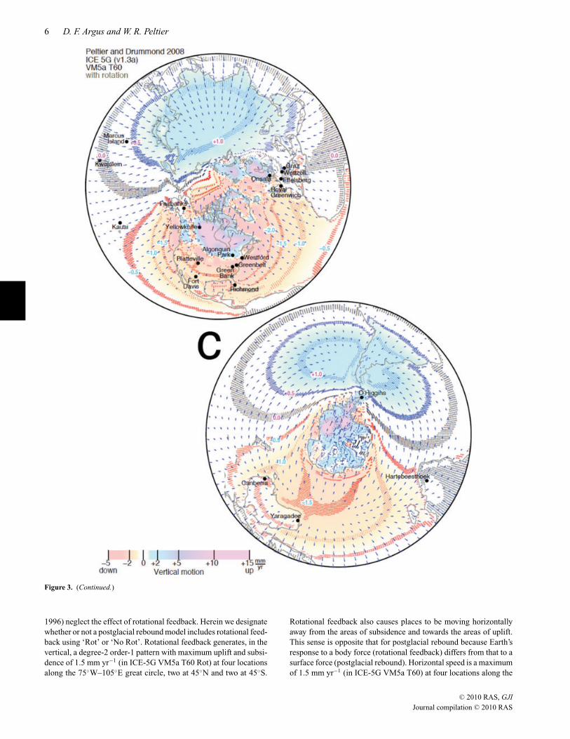
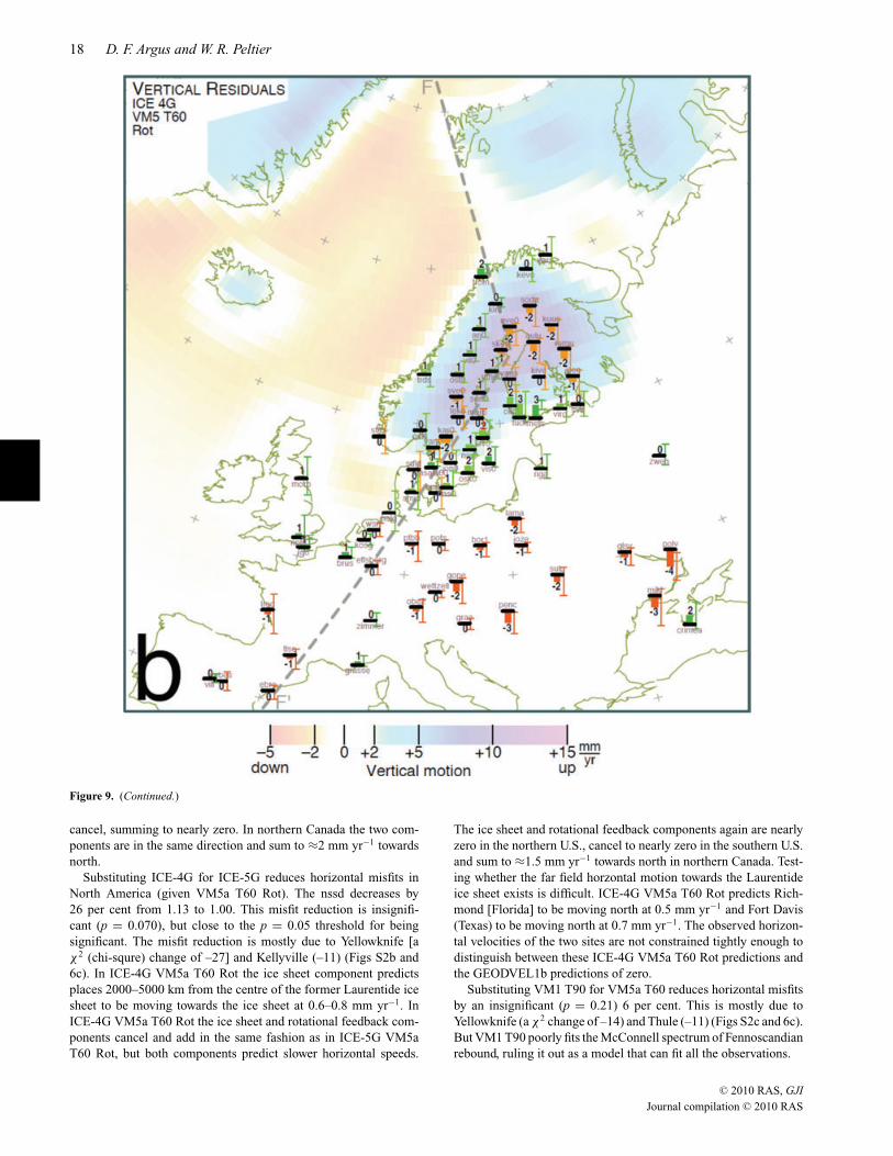
Figure 9. Residuals of the observed vertical rates of places on the Eurasian Plate interior relative to the predictions of model (a) ICE-5G VM5a T60 Rotand (b) ICE-5G VM5a T60 Rot. Green bars show positive residuals, orange bars negative residuals; Residual speeds are given in mm yr−1; Error bars are95 per cent confidence limits; ‘X’s are the predictions of uplift or subsidence in the postglacial rebound model. F–F′ show the location of the profiles in Fig. 10.The colour gradations show, as the legend specifies, the predictions of the postglacial rebound model. See Fig. S3 for the residuals of four other postglacialrebound models.

high-viscosity (10 × 1021 Pa s) layer 40 km thick in place of anelastic layer 90 km thick significantly reduces horizontal misfits inNorth America (Peltier & Drummond 2008). Given ICE-4G Rot,the nssd decreases by a highly significant 70 per cent, from 1.68 to1.00 (Fig. 5, Table 3). The probability p of the misfit falling thismuch by chance is just 6.1 × 10−11. VM5a T60 Rot predicts placesnear the margins of the ice sheet to be moving horizontally moreslowly than in VM2 T90 Rot, and VM5a T60 Rot predicts the NorthAmerican Plate in southern Canada and the United States to be mov-ing horizontally hardly at all, in agreement with the observations(Figs S2b and 6c).

ICE-5G VM5a T60 Rot consists of two components, an icesheet component (Fig. 3a) and a rotational feedback component(Fig. 3b). The ice sheet component predicts places 3000–6500 kmfrom the centre of the former Laurentide ice sheet to be movinghorizontally towards the ice sheet at 1–1.5 mm yr−1. Testing thisprediction is difficult because sites on the North American Plateinterior are not far enough from the ice sheet centre. The rota-tional feedback component predicts a degree-2 order-1 pattern ofhorizontal velocity. In the northern United States the ice sheet androtational feedback components are both nearly zero. In the south-ern United States the two components are in opposite directions and

C© 2010 RAS, GJI




cancel, summing to nearly zero. In northern Canada the two com-ponents are in the same direction and sum to ≈2 mm yr−1 towardsnorth.

Substituting ICE-4G for ICE-5G reduces horizontal misfits inNorth America (given VM5a T60 Rot). The nssd decreases by26 per cent from 1.13 to 1.00. This misfit reduction is insignifi-cant (p = 0.070), but close to the p = 0.05 threshold for beingsignificant. The misfit reduction is mostly due to Yellowknife [aχ 2 (chi-squre) change of –27] and Kellyville (–11) (Figs S2b and6c). In ICE-4G VM5a T60 Rot the ice sheet component predictsplaces 2000–5000 km from the centre of the former Laurentide icesheet to be moving towards the ice sheet at 0.6–0.8 mm yr−1. InICE-4G VM5a T60 Rot the ice sheet and rotational feedback com-ponents cancel and add in the same fashion as in ICE-5G VM5aT60 Rot, but both components predict slower horizontal speeds.

The ice sheet and rotational feedback components again are nearlyzero in the northern U.S., cancel to nearly zero in the southern U.S.and sum to ≈1.5 mm yr−1 towards north in northern Canada. Test-ing whether the far field horzontal motion towards the Laurentideice sheet exists is difficult. ICE-4G VM5a T60 Rot predicts Rich-mond [Florida] to be moving north at 0.5 mm yr−1 and Fort Davis(Texas) to be moving north at 0.7 mm yr−1. The observed horizon-tal velocities of the two sites are not constrained tightly enough todistinguish between these ICE-4G VM5a T60 Rot predictions andthe GEODVEL1b predictions of zero.

Substituting VM1 T90 for VM5a T60 reduces horizontal misfitsby an insignificant (p = 0.21) 6 per cent. This is mostly due toYellowknife (a χ 2 change of –14) and Thule (–11) (Figs S2c and 6c).But VM1 T90 poorly fits the McConnell spectrum of Fennoscandianrebound, ruling it out as a model that can fit all the observations.

C© 2010 RAS, GJI



Figure 10. Observed vertical rates of site motion as a function of angular distance along profile F–F′ (Fig. 11). Blue circles show uplift and red circlessubsidence of VLBI, SLR and permanent GPS sites; open circles show permanent GPS sites of the BIFROST network; Error bars are 95 per cent confidencelimits.

Next, in the vertical evaluation, we compare against VM5a T60Rot because VM2 T90 Rot poorly fits the North America horizontalobservations.

5.4 Vertical North America

Substituting ICE-4G for ICE-5G reduces vertical misfits in NorthAmerica by a significant (p = 0.00096) 42 per cent (given VM5aT60 Rot). The nssd decreases from 1.58 to 1.11. This is mostlydue to Yellowknife (a χ 2 change of –63, and to sites in and nearsouthern Manitoba, including Lac du Bonnet (a χ 2 change of −18),Flin Flon (–17) and many CBN sites (–50 for knra, fard, wina, bmtn,daup, and win5) (two areas circled by blue ellipses in Figs 7a andS3a; and Fig. 8).

Yellowknife [along the north coast of Great Slave Lake, North-west Territories] is observed to be rising at 4.8 ± 1.4 mm yr−1,6 mm yr−1 slower than the ICE-5G prediction and 2 mm yr−1 fasterthan the ICE-4G prediction. The observation is based mainly on12 yr of VLBI data and 10 years of GPS data (Table S1a). There-fore, near Yellowknife the Laurentide ice sheet at LGM was eitherthicker than in ICE-4G and much thinner than in ICE-5G or the icecame off the western part of the Laurentide ice sheet later than inICE-4G or earlier than in ICE-5G.

Places in southern Manitoba (e.g. knra, fard, wina, win5, daupand win5) are observed to be moving vertically very slowly if at all(Fig. S1a). For example, Lac du Bonnet is observed to be rising at0.8 ± 3.1 mm yr−1. In southern Manitoba ICE-5G predicts uplift tobe ≈7 mm yr−1 faster than observed, whereas ICE-4G fits the obser-vations well. Similarly Flin Flon (along the Manitoba-Saskatchewanborder) is observed to be rising at 2.7 ± 2.6 mm yr−1, 6 mm yr−1

slower than the ICE-5G prediction. If we were not to estimate 1logged and 1 unlogged antenna offset, we would find Flin Flon tobe falling at –0.5 mm yr−1.

Therefore we conclude that the 4000-km-thick ice ridge in ICE-5G at LGM extending from north to south across Lake Winnepegdid not exist; there the ice sheet at LGM was ≈2000 km thick asin ICE-4G. This thin ice ridge disagrees with the inference (Peltier2004) from the terrestrial gravity data of Lambert et al. (2001) thatthere was a thick ridge in Manitoba but is consistent with the gravity

data of Pagiatakis & Salib (2003) in Saskatchewan. Given that thegravity rates of Lambert et al. (2001) are based on observationsover just 5 yr, and given the high dispersion in their and Pagiatakis& Salib’s (2003) gravity rates, we believe the terrestrial gravity datado not constrain the vertical rate of motion as strongly as do theGPS data.

Places in northern Manitoba are observed to be rising at≈6 mm yr−1. ICE-5G predicts uplift to be ≈5 mm yr−1 fasterthan observed, whereas ICE-4G predicts uplift to be ≈3 mm yr−1

slower than observed.Churchill (along the west shore of Hudson Bay) is observed

to be rising at 10.2 ± 2.6 mm yr−1, 3 mm yr−1 slower than inICE-5G and 2 mm yr−1 faster than in ICE-4G. Based on observa-tions at Yellowknife, at Churchill, in northern Manitoba, at BakerLake (northwest of Hudson Bay, Nunavut), and at Holman (VictoriaIsland), we deduce that the western part of the Laurentide ice sheetat LGM was intermediate in thickness between ICE-4G and ICE-5G(assuming the timing of the unloading of the ice sheet is constrainedwell by glacial geomorphology).

Places near the northern Alberta–British Columbia border (e.g.gdpr, ftsj and cdpr) are observed to be rising at ≈5 mm yr−1,indicating that there the Laurentide ice sheet at LGM was thickerthan in either ICE-5G or ICE-4G (area circled by red ellipse inFig. 7a). These observations and those at Yellowknife and Holman(Victoria Island) suggest that the Keewatin ice dome at LGM wasnot as thick at the centre but thicker along its flanks than in ICE-5G. We are currently modifying the model of ice sheet thicknessas a function of position and time to fit all the space geodeticobservations.

Many places in Quebec (e.g. Schefferville, Val d’Or, mnc5, injk,lsar and cmou) have positive residuals of roughly 3 mm yr−1 relativeto either ICE-4G or ICE-5G, suggesting that the eastern Laurentideice sheet was slightly thicker at LGM than in either ICE-4G or ICE-5G (area circled by red ellipse in Figs 7a and S3a). Schefferville(along the Labrador–Quebec border) is rising at 9.8 ± 2.1 mm yr−1,2 mm yr−1 faster than predicted by either ICE-4G or ICE-5G. Ob-servations along the Saint Lawrence river (e.g. baie, cnda, stan andpcrt) suggest that at LGM the ice sheet extended farther south-east than in either ICE-4G or ICE-5G. Algonquin Park (Ontario) is

C© 2010 RAS, GJI



Figure 11. Observed horizontal velocities relative to the Eurasian Plate angular velocity in the reference frame minimizing differences with (a) themodel [GEODVEL1b] in which the parts of the plate interiors not near the late Pleistocene ice sheets are rigid, (b) ICE-5G VM5a T60 Rot, (c) theice sheet component of ICE-5G VM5a T60 Rot and (d) the rotational feedback component of ICE-5G VM5a T60 Rot. Red arrows show predicted ve-locities and are omitted where less than 0.5 mm yr−1. Black arrows show well-constrained observed velocities; grey arrows show poorly constrainedobserved velocities. Error ellipses are 95 per cent confidence limits and are filled gold for the tightest constrained velocities (semi major axis less than0.5 mm yr−1), filled yellow for velocities either constrained medium well (semi major axis greater than 0.5 mm yr−1 and less than 0.8 mm yr−1),and are omitted for poorly constrained velocities (semi major axis greater than 0.8 mm yr−1). The predictions in (c) and (d) total to those in (b).See Fig. S5 for model ICE-5G VM2 T90 Rot and the model’s ice sheet and rotational feedback components.

observed to be rising at 1.8 ± 1.1 mm yr−1, just 1 mm yr−1 fasterthan in either ICE-4G or ICE-5G.

VM5a T60 and VM1 T90 fit all the vertical data about equallywell (χ 2 difference of 2; Fig. 5, Table 3). On one hand substitut-ing VM1 T90 for VM5a T60 reduces the vertical misfits in NorthAmerica, decreasing the nssd by an insignificant 8 per cent from

1.111 to 1.032 (χ 2 change of –24). This decrease is due to the ob-servation that several GPS sites in the area of forebulge collapse(mil1, pit1, wis1, sag1, stb1 and pnr1) are observed to be subsidingquickly, as predicted by VM1 T90 (Figs 8 and S3c). On the otherhand Westford, Greenbelt and Green Bank (VLBI and SLR siteswith long histories of observation) are observed to be subsiding

C© 2010 RAS, GJI




very slowly, as predicted by VM5a T60 and Canberra and Hobart(both in Australia), on the opposite side of Earth, are moving ver-tically at rates agreeing better with the Earth’s centre velocity inVM5a T60 than that in VM1 T90. Thus the worldwide vertical ob-servations do not distinguish between VM1 T90 and VM5a T60.This analysis nevertheless illustrates the difficulty in distinguishingbetween postglacial models.

In the GEODVEL1b reference frame the weighted mean verticalrate of 163 places in the United States is subsidence at –1.5 mm yr−1.The weighted root mean square dispersion about this mean is1.6 mm yr−1. The reference frame minimizing differences withICE-4G VM5a T60 Rot gives 0.0–0.2 mm yr−1 more uplift thandoes GEODVEL1b (Figs 7b and S1a).

5.5 Vertical Eurasia

Substituting ICE-5G for ICE-4G reduces vertical misfits in Eurasiaby 33 per cent, decreasing the nssd from 1.32 to 1.00 (given VM5aT60 Rot). This misfit reduction is insignificant (p = 0.077), butmarginally so. The misfit reduction (χ 2 change of –33) is mostlydue to Metsahovi (–21) and Tuoria (−4) (Figs 9a and 9b).

ICE-5G VM5a T60 fits the vertical observations in Eurasia well.Umea, Skelleftea and Sundsvall, at the centre of Fennoscandianrebound, are estimated to be rising at 9–10 mm yr−1 (Fig. S1b).Tromso, Metsahovi, Kiruna and Onsala are constrained the tightest,and strongly constrain Fennoscandian rebound. Metsahovi (Finland)is estimated to be rising at 4.0 ± 1.3 mm yr−1, in agreement withICE-5G but 3 mm yr−1 faster than in ICE-4G.

C© 2010 RAS, GJI



Figure 12. Change in equivalent water thickness estimated from GRACE observations from 2002 April to 2007 January from (CSR) Center for SpaceResearch model RL04 less surface water change in hydrology model (GLDAS) Global Land Data Assimilation System and less the predictions of postglacialrebound models (left-hand panel) ICE-4G VM2 T90 Rot and (right-hand panel) ICE-5G VM2 T90 Rot. Stokes coefficients of degree-1, degree-2 order-0, anddegree-2 order-1 are omitted in the calculation; the degree-2 order-2 coefficient and higher coefficients are included. The degree-2 order-0 coefficient is nottightly constrained by GRACE; the degree-2 order-1 coefficient records current ice mass loss in Alaska, Antarctica, Greenland, and elsewhere that is not in thepostglacial rebound models. A Gaussian half width of 500 km is used. The analysis is identical to that in Peltier (2009, fig. 5).

Figure 13. Uplift observed with GPS, VLBI, SLR and DORIS is plotted against terrestrial estimates of gravity change. Error bars are 1 sigma. GRACE andterrestrial estimates of gravity must be interpreted differently. GRACE observations of gravity are at a reference ellipsoid; terrestrial observations of gravityare at Earth’s surface. Earth’s surface is rising in Canada, causing a gravimeter to be moving away from Earth’s centre, decreasing gravity at the site. Wahret al. (1995) estimate this gravity change to be –1 mGal per 6.5 mm yr−1 uplift (bottom horizontal scale). If this ratio were exact, if the space and terrestrialobservations were exact, and if Earth’s water changes in Canada were negligible, then all the data would fall along the 45◦ dashed line. Rangelova & Sideris(2008) find that a ratio of –1 mGal per 5.6 mm yr−1 uplift minimizes differences between the terrestrial gravity and the Canada Base Network data. For moreon the ratio see de Linage et al. (2007).

C© 2010 RAS, GJI



Table 3. Significance of differences between models.

Element 1 Element 2 Given �χ2 Nssd1 Nssd2 F dof p

North America HorizontalVM2 T90 VM5a T60 ICE-5G Rot −918.9 2.609 1.126 2.317 619.7 3.2 × 10−25

VM2 T90 VM5a T60 ICE-4G Rot −423.1 1.682 1.000 1.682 619.7 6.1 × 10−11

ICE-5G ICE-4G VM5a T60 Rot −78.4 1.126 1.000 1.126 619.7 0.070VM5a T60 VM1 T90 ICE-4G Rot −37.3 1.000 0.939 1.065 619.7 0.21

North America VerticalICE-5G ICE-4G VM5a T60 Rot −146.8 1.580 1.111 1.422 313.1 0.00096VM1 T90 VM5a T60 ICE-4G Rot −25 1.111 1.032 1.076 313.1 0.26

Eurasia VerticalICE-5G ICE-4G VM5a T60 Rot −33.1 1.325 0.995 1.332 100.2 0.077

Eurasia HorizontalVM2 T60 VM5a T90 ICE-5G Rot −4.2 0.555 0.534 1.040 194.2 0.39

All VerticalVM5a T60 VM1 T90 ICE-4G Rot −2.5 1.291 1.286 1.004 457.8 0.48No Rot Rot ICE-4G VM5a T60 −26.5 1.344 1.286 1.045 457.8 0.32

All HoriztonalRot No Rot ICE-4G VM5a T60 −22.6 1.038 1.013 1.025 882.7 0.36

Category Rigid HorizontalICE-4G VM5a T60 Rot GEODVEL1b −13.5 1.225 1.197 1.023 483.3 0.40ICE-4G VM5a T60 No Rot GEODVEL1b −36.4 1.272 1.197 1.063 483.3 0.25Rotational feedback component GEODVEL1b −71.9 1.346 1.197 1.124 483.3 0.10

of ICE-4G VM5a T60

Notes: Each row describes the misfit difference between two postglacial rebound models. For example (row2), substituting VM5a T60 for VM2 T90 reducesthe misfit of the horizontal observations (χ2 decrease of 423.1 given ICE-5G Rot). The normalized sample standard deviation decreases from 1.682 to 1.000.There are 619.7 degrees of freedom (dof), computing degrees of freedom using a formula (dof = ndat – imp) in which we substitute data importance (imp) forthe number of parameters in the usual formula [Bevington 1969, p. 89]. F in an F-test is 1.682, indicating the misfit reduction to be statistically significant[probability (p) = 6.1 × 10−11].

Onsala is observed to be rising at 2.3 ±1.1 mm yr−1.In the GEODVEL1b reference frame the weighted mean vertical

rate of 42 places in continental Europe, Asia and England is subsi-dence at –0.8 mm yr−1. The weighted root mean square dispersionabout this mean is just 0.8 mm yr−1. The reference frame mini-mizing differences with ICE-5G VM5a T60 Rot gives 0.3 mm yr−1

more uplift than does GEODVEL1b (Figs 9a and S1b).

5.6 Horizontal Eurasia

In the reference frame (GEODVEL1b) minimizing the horizontaldeformation of the parts of the plate interiors not near the ice sheets,the Eurasian Plate interior appears to be nearly rigid except forplaces near the former Fennoscandian ice sheet (Fig. 11a). Theweighted root mean square residual speed of places not near theFennoscandian ice sheet is 0.6 mm yr−1. Places along the marginsof the Fennoscandian ice sheet are moving laterally away from theice centre. Onsala is moving south at 1.0 ± 0.5 mm yr−1, Metsahovisoutheast at 0.9 ± 0.6 mm yr−1, Tromso northwest at 1.3 ± 0.5 mmyr−1 and Kiruna northwest at 1.3 ± 0.6 mm yr−1.

We omit Ny Alesund and Hofn because they are moving in elas-tic response to current ice mass loss that is not in the postglacialrebound models. Ny Alesund, along the west coast of Spitsbergenisland 110 km east of the Eurasia–North America Plate boundary,is rising at 7.2 ± 1.4 mm yr−1, in response to ice loss from glaciersto its east (Hagedoorn & Wolf 2003; Sato et al. 2006; Kohler et al.2007) but is moving horizontally at an insignificant speed relativeto the Eurasian Plate. Hofn, along the east coast of Iceland 100 km

east of the Eurasia–North America Plate boundary (Geirsson et al.2006), is rising at 13.4 ± 3.1 mm yr−1 and moving east relative tothe Eurasian Plate at 4.5 ± 1.4 mm yr−1, in elastic response to iceloss from Vatnajokull glacier (Pagli et al. 2007).

Substituting VM5a T60 for VM2 T90 insignificantly (p = 0.39)reduces horizontal misfits in Eurasia (Fig. 5, Table 3). Given ICE-5G Rot, the nssd decreases by 4 per cent, from 0.55 to 0.53.These small values of nssd suggest that the uncertainties in thehorizontal velocities in Eurasia are underestimated by a factor ofnearly 2.

The predictions of ICE-5G VM5a T60 Rot consist of three parts.The rotational feedback component predicts Europe to be movingeast at ≈1 mm yr−1 (Fig. 11d). The Laurentide part of the ice sheetcomponent predicts Europe to be moving northwest, at speeds in-creasing from ≈0.8 mm yr−1 in southeast Europe to ≈1.3 mm yr−1

in Fennoscandia (Fig. 11c). The Fennoscandian part of the icesheet component predicts the margins of the Fennoscandian icesheet to be moving laterally away from the ice centre at roughly≈1 mm yr−1.

Because the Eurasian Plate velocity in ICE-5G VM5a T60 Rotmust adjust to fit the rotational feedback component and the Lau-rentide part of the ice sheet component, the angular velocity min-imizing differences with ICE-5G VM5a T60 differs from that inGEODVEL1b. Testing whether the rotational feedback and Lauren-tide ice sheet components exist is difficult because the predictionschange slowly across the part of the Eurasian Plate interior havingsites.

ICE-5G VM5a T60 Rot predicts Tromso to be moving northat 0.8 mm yr−1, more slowly than observed (Fig. 11b). And

C© 2010 RAS, GJI



ICE-5G VM5a T60 Rot predicts Onsala to be moving northeastat 0.4 mm yr−1, more northeast than observed.

5.7 Rotational feedback

Rot and No Rot fit all the data about equally well (Fig. 5, Table 3).Given ICE-4G VM5a T60, substituting ‘No Rot’ for ‘Rot’ increasesvertical misfits by an insignificant 4 per cent and reduces horizontalmisfits by an insignificant 2 per cent. Thus the data cannot distin-guish between models with and without rotational feedback, in thevertical because the velocity of Earth’ centre is uncertain, and inthe horizontal because the areas of the plate interiors having geode-tic sites is not large enough to detect the small differences in thepredictions of rotational feedback going across the plate interiors.

5.8 GEODVEL1b versus ICE-4G VM5a Rot: are theparts of the plates not near the ice sheets deforming?

To further evaluate to what degree the parts of the plates not nearthe former ice sheets are deforming laterally, we estimate the an-gular velocities of the plates and the velocity of Earth’s centre bestfitting the horizontal velocities of places in Category Rigid (Table 3,bottom 3 rows).

Substituting GEODVEL1b for ICE-4G VM5a T60 Rot reducesmisfits by an insignificant (p = 0.40) 2 per cent.

What if the rotational feedback component were not in the post-glacial rebound model? Substituting GEODVEL1b for ICE-4GVM5a T60 No Rot reduces misfits by an insignificant (p = 0.25)6 per cent. Of the total χ 2 change of –36, this is due mostly toplaces on the Pacific Plate (χ 2 change of –20, of which Chathamisland contributes –13), on the Antarctica Plate (χ 2 change of –18,of which Kerguelen contributes –13), and on the Nubian Plate (χ 2

change of –10, of which Maspalomas contributes –8). The totalmisfit reduction is insignificant; nevertheless these are the placesat and near which more data can begin to discriminate between thetwo models.

What if we were to neglect the ice sheet component? SubstitutingGEODVEL1b for a model in which the parts of the plates not nearthe former ice sheets are deforming only in rotational feedbackreduces misfits by an insignificant (p = 0.10) 12 per cent. Of thetotal χ 2 change of –72, this is due mostly to places on the NorthAmerican Plate (χ 2 change of –76).

Thus the horizontal data cannot distinguish between a modelin which the parts of the plate not near the former ice sheets arerigid and a model in which these areas are moving laterally eitheras predicted by rotational feedback, or towards the Laurentide icesheet in the far field or both.

6 D I S C U S S I O N

Tamisiea et al. (2007), Paulson et al. (2007) and Peltier (2009) findGRACE observations of gravity increase from 2002 to 2006 to beconsistent with ICE-5G and with there being distinct ice domeseast and west of Hudson Bay. In particular Peltier’s (2009) com-parison suggests that the GRACE observations are more consistentwith the larger size of the western Laurentide ice sheet in ICE-5Gthan with the smaller size in ICE-4G model (Fig. 12). Two decadesago Dyke & Prest (1987) suggested, on the basis of glacial geo-morphology, that ice domes existed both west and east of HudsonBay, as later suggested on the basis of space geodesy by Arguset al. (1999) & Peltier (2002b). In this study, we find that the GPS,VLBI, SLR and DORIS data suggest that the Laurentide ice sheet

at LGM was intermediate between that in ICE-5G and ICE-4G.Rangelova & Sideris (2008) also find that terrestrial gravity andthe Canadian Base Network are more consistent with ICE-4G, butthat the GRACE data are more consistent with ICE-5G. We expectthat we can construct a model that is intermediate between ICE-4G and ICE-5G and that well fits both the GRACE observationsand GPS, VLBI, SLR, and DORIS data that are analyzed herein,given that the latter data well constrain the ice sheet thickness alongthe southern limit of the western Laurentide ice sheet but not nearits centre except at Yellowknife. The western Laurentide ice sheetmust be nearly as massive as that in ICE-5G to fit the GRACEdata, but the ice must be distributed more broadly across northwest-ern Canada in order to also fit the GPS, VLBI, SLR and DORISobservations.

Tregoning et al. (2009, fig. 5) find groundwater gain at Flin Flonand west of Hudson Bay to significantly affect their inference ofvertical uplift from GRACE gravity obervations. But we find (F.W.Landerer, personal communication, 2009) that elastic deformationgenerated by groundwater gain or loss from 2003 to 2008 [computedfrom GLDAS data using eq. (3) of Tregoning et al. (2009)] in mostplaces amounts to less than 1 mm yr−1 of subsidence or uplift,and that groundwater gain at Flin Flon causes it to subside at just0.2 mm yr−1.

Using observations from absolute and relative gravimeters from1961 to 1999, Pagiatakis & Salib (2003) estimate rates of surfacegravity change at 64 sites in Canada. In general these terrestrialgravity observations are also consistent with an ice model that isintermediate between ICE-4G and ICE-5G and with there beingdistinct ice domes east and west of Hudson Bay (Pagiatakis & Salib2003, fig. 6). However, the large dispersion in the estimated terres-trial gravity rates (Fig. 13), as evident in the many local maxima andminima on their map (Pagiatakis & Salib 2003, fig. 7), as well asthe fact that the gravity rates are sensitive to fluctuations in ground-water hydrology, make them difficult to interpret. For example, thegravity data suggest Yellowknife to be rising at 7.7 ± 0.7 mm yr−1,faster than observed with mainly VLBI and GPS data and nearer theICE-5G prediction; however these gravity data also suggest Calgaryto be rising at 5.3 ± 2.4 mm yr−1, in disagreement with the observedvertical motion of nearly zero.

Using tide gauge data from 1860 to 2000, Mainville & Craymer(2005) estimate rates of lake level change at 55 sites along the shoresof the Great Lakes. Although the northern shores of the Great Lakesappear to be rising and the southern shores subsiding, the tide gaugedata poorly constrain the zero contour in the vertical motion ofEarth’s surface because of anthropogenic management of the waterlevels. (For example, gates, locks, and power canals along the SaintMary River are used to control the flow of water between LakeSuperior and Lake Huron.) This is evident in the observation thatcontours of the rate of rise of water level do not line up between LakeSuperior on the west and Lakes Huron and Michigan on the east(Mainville & Craymer 2005, fig. 5). The data constrain the gradientin the vertical motion of Earth’s surface assuming that the waterlevel conforms to a gravitational equipotential surface. The tidegauge data suggest this gradient to be 1.5 mm yr−1/100 km goingfrom NNE to SSW across Lake Superior, three times steeper than thegradient of ≈0.6 mm yr−1 going from NNE to SSW beginning alongthe northern shore of the North Channel of Lake Huron and endingat the southern tip of Lake Michigan (water levels are not beingmanipulated in the Straits of Mackinac between Lake Huron andLake Michigan). It is impressive that the tide gauge data record thisflattening of the vertical gradient along a traverse from the ice sheetcentre that is predicted by the postglacial rebound models. ICE-4G

C© 2010 RAS, GJI



VM1 T90 Rot (the prediction is 1.4 mm yr−1/100 km) fits the steepgradient across Lake Superior better than does ICE-4G VM5a T60Rot (the prediction is 0.6 mm yr−1/100 km); either of the two modelsfits the gentle gradient across Lakes Huron and Michigan (the VM1T90 prediction is 0.9 mm yr−1/100 km; the VM5a T60 prediction is0.5 mm yr−1)/100 km. (The predicted gradient in relative sea levelis 12 per cent less than the predicted gradient in vertical motion;this does not change the conclusion we state next.) We agree withthe inference of Mainville & Craymer (2005) that the tide gaugedata favour ICE-4G VM1 T90 Rot over ICE-4G VM5a T60 Rot,but believe that the tide gauge data do not constrain the verticalgradient well enough to conclusively distinguish between the twomodels. [Mainville & Craymer (2005) compared against ICE-4GVM2 T90 not ICE-4G VM5a T60, but because VM5a is a three-layer approximatiton to VM2 in the mantle, the vertical gradient issimilar in the two models (Fig. 8).]

Estimates of the location of the zero isoline separating upliftfrom subsidence, and the width of the subsiding belt around the latePleistocene ice sheets depend strongly on the velocity of Earth’scentre. In North America the zero isoline and subsiding belt alsodepend on the strength of rotational feedback; in Europe the two donot depend on the strength of rotational feedback (Fig. 3b).

In North America Sella et al. (2007), assuming Earth’s cen-tre to be the velocity of CM in ITRF2000, find the zero isolineto cut through the northern Great Lakes, towards the east nearthe Canada–United States border, and towards the west throughManitoba, Saskatchewan, and Alberta. We find, given the velocityof Earth’s centre in ICE-4G VM5a T60 Rot, the zero isoline to benear theirs. The model suggests that all of the United States is sub-siding at 0.5–2 mm yr−1, mostly due to the subsidence generatedby rotational feedback.

In Europe Nocquet et al. (2005), assuming Earth’s centre to bethe velocity of CM in ITRF2000, maintain that in Europe there isa belt 900 km wide that is subsiding at up to 1.5 mm yr−1 and thatextends from the north coast of Germany to Italy. We find, given thevelocity of Earth’s centre in ICE-5G VM5a T60 Rot, that most ofEurope is moving vertically at ≈0 mm yr−1; near Denmark there isa belt roughly 300 km wide subsiding at 0.5–1.5 mm yr−1 (Fig. 9a).

7 C O N C LU S I O N S

(1) The vertical observations in North America show that, rel-ative to ICE-5G, the Laurentide ice sheet at LGM was (i) muchthinner in southern Manitoba, (ii) thinner near Yellowknife (North-west Territories), (iii) thicker in eastern and southern Quebec and(iv) thicker along the northern British Columbia–Alberta border, orthat ice was unloaded from these areas later (thicker) or earlier (thin-ner) than in ICE-5G. The data indicate that the western Laurentideice sheet was intermediate in mass between ICE-5G and ICE-4G.The vertical observations and GRACE gravity data together suggestthat the western Laurentide ice sheet was nearly as massive as that inICE-5G but distributed more broadly across northwestern Canada.

(2) Substituting VM5a T60 (Peltier & Drummond 2008) forVM2 T90, that is, introducing into the lithosphere at its base alayer with a high viscosity of 10 × 1021 Pa s, greatly improves thefit of the horizontal observations in North America. ICE-4G VM5aT60 Rot predicts the North American Plate to be deforming slowlyhorizontally, in agreement with the data.

(3) ICE-5G VM5a T60 Rot well fits the vertical and horizontalobservations in Europe.

(4) The rotational feedback component of the models predictsa degree-2 order-1 pattern, with maximum uplift, maximum sub-

sidence, and maximum horizontal movement of 1.5 mm yr−1 inICE-5G and 1 mm yr−1 in ICE-4G (given VM5a T60 Rot). Theice sheet component of VM5a T60 Rot predicts places there tobe in far field horizontal motion towards the Laurentide ice sheet(at 1–1.5 mm yr−1 at distances 3000 to 6500 km from the Lau-rentide ice sheet given ICE-5G, and at 0.9–1.2 mm yr−1 at dis-tances 2000–5000 km given ICE-4G). The data cannot distin-guish between models with and without rotational feedback, inthe vertical because the velocity of Earth’ centre is uncertain, andin the horizontal because the areas of the plate interiors havinggeodetic sites is not large enough to detect the slow differencesin the predictions of rotational feedback going across the plateinteriors.

A C K N OW L E D G M E N T S

We are grateful to Dr Michael Craymer and scientists at NationalResources Canada for providing estimates of the velocities of sitesin the Canadian Base Network. We are grateful to Dr RosemarieDrummond (University of Toronto) for collating the predictions ofthe postglacial rebound models. We thank John Beavan, KosukiHeki and an anonymous reviewer for their careful reviews. Partof this research was performed at Jet Propulsion Laboratory, Cal-ifornia Institute of Technology, under contract with NASA. Thisresearch is also a contribution to the work of the Polar ClimateStability Network which is funded by the Canadian Foundation forClimate and Atmospheric Sciences and a consortium of Canadianuniversities Additional support was provided by NSERC DiscoveryGrant A9627.

R E F E R E N C E S

Altamimi, Z., Sillard, P. & Boucher, C., 2002. ITRF2000: a new release ofthe international terrestrial reference frame for earth science applications,J. geophys. Res., 107(B10), 2214, doi:10.1029/2001JB000561.

Altamimi, Z., Collilieux, X., Legrand, J., Garayt, B. & Boucher, C., 2007.ITRF2005: a new release of International Terrestrial Reference Framebased on time series of station positions and Earth Orientation Parameters,J. geophys. Res., 112, B004949, doi:10.1029/2007JB004949.

Argus, D.F., 1996. Postglacial uplift and subsidence of earth’s surface usingVLBI geodesy: on establishing vertical reference, Geophys. Res. Lett.,23, 973–976.

Argus, D.F., 2007. Defining the translational velocity of the referenceframe of Earth, Geophys. J. Int., 169, 830–838, doi:10.1111/j.1365-246X.2007.03344.x.

Argus, D.F. & Gordon, R.G., 1996. Tests of the rigid-plate hypothesis andbounds on intraplate deformation using geodetic data from very longbaseline interferometry, J. geophys. Res., 101, 13 555–13 572.

Argus, D.F. & Gross, R.S., 2004. An estimate of motion between the spin axisand the hotspots over the past century, Geophys. Res. Lett., 31, LO6614,doi:10.1029/2004GL019657.

Argus, D.F., Peltier, W.R. & Watkins, M.M., 1999. Glacial isostatic adjust-ment observed using very long baseline interferometry and satellite laserranging, J. geophys. Res., 104, 29 077–29 083.

Argus, D.F., Gordon, R.G., Heflin, M.B., Eanes, R.J., Ma, C., Willis, P.,Peltier, W.R. & Owen, S.E., 2010. The angular velocity of the plates andthe velocity of Earth’s center from space geodesy, Geophys. J. Int., 180,doi:10.1111/j.1365-246X.2010-x.

Bevington, P., 1969. Data Reduction and Error Analysis for the PhysicalSciences, McGraw-Hill Book Company, New York.

Bos, M.S., Fernandes, R.M.S., Williams, S.D.P. & Bastos, L., 2008. Fasterrror analysis of continuous GPS observations, J. Geodyn., 82, 137–166,doi:10.1007/s00190-007-0165-x.

C© 2010 RAS, GJI



de Linage, C., Hinderer, J. & Rogister, Y., 2007. A search for the ratiobetween gravity variation and vertical displacement due to a surface load,Geophys. J. Int., 171, 986–994, doi:10.1111/j.1365-246X.2007.03613x.

Dyke, A.S. & Prest, V.K., 1987. Late Wisconsinian and Holocene Historyof the Laurentide ice sheet, Geographie physique et Quaternaire 41,237–263.

Geirsson, H. et al., 2006. Current plate movements across the Mid-Atlanticridge determined from 5 years of continuous GPS measurements in Ice-land, J. geophys. Res., 111, B09407, doi:10.1029/2005JB003717.

Gross, R.S. & Vondrak, J., 1999. Astrometric and space-geodetic observa-tions of polar wander, Geophys. Res. Lett., 26, 2085–2088.

Hagedoorn, J.M. & Wolf, D., 2003. Pleistocene and Recent deglaciationin Svalbard: implications for tide-gauge, GPS and VLBI measurements,J. Geodyn., 35, 415–423.

Heki, K., 1996. Horizontal and vertical crustal movements from three-dimensional very long baseline interferometry kinematic reference frame:implication for the reversal time scale revision, J. geophys. Res., 101,3187–3198.

James, T.S., Gowan, E.J., Wada, I. & Wang, K.L., 2009. Viscosity of theasthenosphere from glacial isostatic adjustment and subduction dynamicsat the northern Cascadia subduction zone, British Columbia, Canada,J. geophys. Res., 114, B04405, doi:10.1029/2008JB006077.

Johansson, J.M. et al., 2002. Continuous GPS measurements of post-glacial adjustment in Fennoscandia: 1. Geodetic results, J. geophys. Res.,107(B8), 2157, doi:10.1029/2001JB000400.

Kaufmann G. & Lambeck, K., 1997. Glacial isostatic adjustment and theradial viscosity profile from inverse modeling, J. geophys. Res., 107, 2280,doi:10.1029/2001JB000941.

Kohler, J., James, T.D., Murray, T., Nuth, C., Brandt, O., Barrand,N.E., Aas, H.F. & Luckman, A., 2007. Acceleration in thinningrate on western Svalbard glaciers, Geophys. Res. Lett., 34, L18502,doi:10.1029/2007GL030681.

Kogan, M.K. & Steblov, G.M., 2008. Current global kinematics from GPS(1995–2007) with the plate-consistent reference frame, 2008. J. geophys.Res., 113, B04416, doi:10.1029/2007JB005353.

Lambert, A., Courtier, N., Sasagawa, G.S., Klopping, F., Winester, D.,James, T.S. & Liard, J.O., 2001. New constraints on Laurentide post-glacial rebound from absolute gravity measurements, Geophys. Res. Lett.,28, 2109–2112.

Leventer, A. et al., 2006. Marine sediment record from East Antarcticamargin reveals dynamics of ice-sheet recession, GSA Today, 16(12), 4–10,doi:10.1130/GSAT01612A.1.

Lidberg, M., Johansson, J.M., Scherneck, H.G. & Davis, J.L., 2007. Animproved and extended GPS-derived 3D velocity field of the glacialisostatic adjustment (GIA) in Fennoscandia, J. Geodyn., 81, 213–230,doi:10.1007/s0019000601024.

Mainville, A. & Craymer, M.R., 2005. Present-day tilting of the GreatLakes region based on water level gauges, GSA Bull., 117, 1070–1080,doi:10.1130/B25392.1.

McCarthy, D.D. & Petit, G., 2004. IERS Technical Note Number 32, In-ternational Earth Rotation and Reference Systems Service Conventions(2003), Frankfurt.

Milne, G.A., Davis, J.L., Mitrovica, J.X., Scherneck, H.G., Johansson, J.M.,Vermeer, M. & Kouivula, H., 2001. Space-geodetic constraints on glacialisostatic adjustment in Fennoscandia, Science, 291, 2381–2385.

Mitrovica, J.X., Wahr, J., Matsuyama, I. & Paulson, A., 2005. The ro-tational stability of an ice-age earth, Geophys. J. Int., 161, 491–506,doi:10.1111/j.1365-246X.2005.02609.x

Nocquet, J.M., Calais, E. & Parsons, B., 2005. Geodetic constraints onglacial isostatic adjustment in Europe, Geophys. Res. Lett., 32, L06308,doi:10.1029/2004GL022174.

Pagiatakis, S.D. & Salib, P., 2003. Historical relative gravity observationsand the time rate of change of gravity due to postglacial rebound and othertectonic movements in Canada, J. geophys. Res., 108(B9), 2406, B92406,doi:10.1029/2001JB001676.

Pagli, C., Sigmundsson, F., Lund, B., Sturkell, E., Geirsson, H., Einarsson,P., Arnadottir, T. & Hreinsdottir, S., 2007. Glacio-isostatic deformationaround Vatnajokull ice cap, Iceland, induced by recent climate warming:

GPS observations and finite element modeling, J. geophys. Res., 112,B08405, doi:10.1029/2006JB004421.

Paulson, A., Zhong, S. & Wahr, J., 2007. Inference of mantle viscosity fromGRACE and relative sea level data, Geophys. J. Int., 171, 497–508.

Peltier, W.R., 1986. Deglaciation-induced vertical motion of the NorthAmerican continent and transient lower mantle rheology, J. geophys. Res.,91, 9099–9123.

Peltier, W.R., 1994. Ice age paleotopography, Science, 265, 195–201.Peltier, W.R., 1996. Mantle viscosity and ice-age ice sheet topography,

Science, 273, 1359–1364.Peltier, W.R., 2002a. Global glacial isostatic adjustment: paleogeodetic and

space-geodetic tests of the ICE-4G (VM2) model, J. Quater. Sci., 17,491–510.

Peltier, W.R., 2002b. On the eustatic sea level history: Last Glacial Maximumto Holocene, Quater. Sci. Rev., 21, 377–396.

Peltier, W.R., 2004. Global glacial isostasy and the surface of the ice-ageearth: the ICE-5G (VM2) model and GRACE, Ann. Rev. Earth planet.Sci., 32, 111–149.

Peltier, W.R., 2005. On the hemispheric origins of meltwater pulse 1a,Quater. Sci. Rev., 24, 1655–1671, doi:10.1016/j.quascirev.2004.06.023.

Peltier, W.R., 2007. History of earth rotation, Treat. Geophys., 9, 243–293.Peltier, W.R., 2009. Closure of the budget of global sea level rise over the

GRACE era: the importance and magnitudes of the required correctionsfor global glacial isostatic adjustment, Quarter. Sci. Rev., 28, 1658–1674,doi:10.1016/j.quascirev.2009.04.004.

Peltier, W.R. & Drummond, R., 2008. Rheological stratifcation of the litho-sphere: a direct inference based upon the geodetically observed pattern ofglacial isostatic adjustment of the North American continent, Geophys.Res. Lett., 35, L16314, doi:10.1029/2008GL034586.

Peltier, W.R. & Fairbanks, R.G., 2006. Global glacial ice volume and LastGlacial Maximum duration from an extended Barbados sea level record,Quarter. Sci. Rev., 25, 3322–3337.

Peltier, W.R. & Luthcke, S.B., 2009. On the origins of Earth rotationalanomalies: new insights on the basis of both “paleogeodetic” data andGravity Recovery and Climate Experiment (GRACE) data, J. geophys.Res., 114, B11405, doi:10.1029/2009JB006352.

Rangelova, E. & Sideris, M.G., 2008. Contributions of terrestrial andGRACE data to the study of the secular geoid changes in North America,J. Geodyn., 46, 131–143, doi:10.1016/j.jog.2008.03.006.

Sato, T., Okuno, J., Hinderer, J., MacMillan, D.S., Plag, H.-P., Francis,O., Falk, R. & Fukuda, Y., 2006. A geophysical interpretation of thesecular displacement and gravity rates observed at Ny-Alesund, Svalbardin the Arctic–effects of post-glacial rebound and present-day ice melting,Geophys. J. Int., 165, 729–743.

Sella, G.F., Stein, S., Dixon, T.H., Craymer, M., James, T.S., Mazzotti,S. & Dokka, R.K., 2007. Observations of glacial isostatic adjustmentin “stable” North America with GPS, Geophys. Res. Lett., 34, L02306,doi:10.1029/2006GL027081.

Solheim, L.P. & Peltier, W.R., 1994. Avalanche effects in phase transitionmodulated thermal convection: a model of Earth’s mantle, J. geophys.Res., 99, 6997–7018.

Stephenson, E.R. & Morrison, L.V., 1995. Long term fluctuations in theEarth’s rotation: 700 B.C. to A.D. 1990, Phil. Trans. R. Soc. Lond., Ser.A, 351, 165–202.

Svendsen, J.I. & 30 others, 2004. Late Quaternary ice sheet his-tory of northern Eurasia, Quater. Sci. Rev., 23, 1229–1271,doi:10.1016/quascirev.2003.12.008.

Tamisiea, M.E., Mitrovica, J.X. & Davis, J.L., 2007. GRACE gravity con-strain ancient ice geometries and continental dynamics over Laurentia,Science, 24, 881–883, doi:10.1126/science.1137157.

Tregoning, P., Ramillien, G., McQueen, H. & Zwartz, D., 2009. Glacial iso-static adjustment and nonstationary signals observed by GRACE, J. geo-phys. Res., 14, B06406, doi:10.1029/2008JB006161.

Turcotte, D.L. & Schubert, G., 1982. Geodynamics,, Cambridge UniversityPress, Cambridge.

Wahr, J., DaZhong, H. & Trupin, A., 1995. Predictions of vertical upliftcaused by changing polar ice volumes on a viscoelastic earth, Geophys.Res. Lett., 22, 977–980.

C© 2010 RAS, GJI



Williams, S.D.P., Bock, Y., Fang, P., Jamason, P., Nikolaidis, R.M.,Prawirodirdjo, L., Miller, L. & Johnson, D.J., 2004. Error analysis ofcontinous GPS position time series, J. geophys. Res., 109, B03412,dois:10.1029/2003JB002741.

A P P E N D I X A : P O L A R M O T I O NA N D T H E P O L E T I D E

Earth’s spin axis is moving relative to the surface geography ofEarth; solid Earth is deforming elastically and viscously in response.The spin axis movement consists mostly of three parts.

(1) A forced wobble having an amplitude of 0.1 arcsec (3 m) anda period of 1 yr,

(2) A free Chandler wobble having an amplitude varying from0.1 to 0.2 arcsec (3–6 m) and a period of 433 d.

(3) The secular polar wander, a mean velocity of 0.0035 arc-sec yr−1 along the 79◦W meridian.

Following the IERS 2003 conventions (McCarthy & Petit 2004),geodesists estimate site positions after subtracting away Earth’s elas-tic response to the forced and free Chandler wobbles, but not Earth’sresponse to polar wander. That is, geodesists correct for the pole tideby subtracting away the effect of all polar motions except secularpolar wander at 0.0040 arcsec yr−1 towards 78.1◦W.

S U P P O RT I N G I N F O R M AT I O N

Additional Supporting Information may be found in the online ver-sion of this article:

Figure S1. (a) Observed vertical rates of motion of places in NorthAmerica in GEODVEL1b; Blue bars show uplift, red bars subsi-dence; Speeds are given in mm yr−1; Error bars are 95 per centconfidence limits. The colour gradations show, as the legend spec-ifies, the predictions of postglacial rebound model ICE-5G VM2T90 Rot. Deeper shades of blue and red are sites on the interiorof the North American Plate used to constrain postglacial rebound;lighter shades of blue and red are sites omitted because either theyare in the deforming zone between plate interiors or they are out-liers in the vertical or horizontal. When we evaluate the postglacialrebound models we omit places west of the east edge of the RockyMountains because they are not on the interior of the North Amer-ican Plate, and we omit places along the north shore of the Gulf

of Mexico are subsiding in response to a phenomenon other thanpostglacial rebound. Omitted places in southeastern Alaska risingin elastic response to current glacier unloading not in the postglacialrebound model. In the vertical observation illustrations (Figures S1aand S1b) the observed velocity is the estimated vertical componentof ub in the GEODVEL1b inversion. (b) Observed vertical rates ofmotion of places in Eurasia in GEODVEL1b; blue bars show uplift,red bars subsidence; Speeds are given in mm yr−1; Error bars are95 per cent confidence limits. The colour gradations show, as thelegend specifies, the predictions of postglacial rebound model ICE-5G VM2 T90 Rot. Deeper shades of blue and red are sites on theinterior of the Eurasian Plate used to constrain postglacial rebound;lighter shades of blue and red are sites omitted because either theyare in the deforming zone between plate interiors or they are out-liers in the vertical or horizontal. When we evaluate the postglacialrebound models we omit places west of the north edge of the Alpsbecause they are not on the interior of the Eurasian Plate. Observedvertical rates are in the reference frame in which the velocity ofEarth’s centre is estimated assuming [Argus (2007), model HORI]the parts of the plate interiors not near the late Pleistocene ice sheetsare not moving horizontally relative to (CE) the mass centre of solidEarth.Figure S2. Identical to Fig. 6 for models (a) ICE-5G VM2 T90Rot, (b) ICE-5G VM5a T60 Rot (c) ICE-4G VM1 T90 Rot and (d)ICE-4G VM5a T60 No Rot.Figure S3. Identical to Fig. 7 for models (a) ICE-5G VM2 T90Rot, (b) ICE-4G VM2 T90 Rot (c) ICE-4G VM1 T90 Rot and (d)ICE-4G VM5a T60 No Rot.Figure S4. Identical to Fig. 9 for models (a) ICE-5G VM2 T90Rot, (b) ICE-4G VM2 T90 Rot, (c) ICE-5G VM1 T90 Rot and (d)ICE-5G VM5a T60 No Rot.Figure S5. Identical to Fig. 11 for (a) ICE-5G VM2 T90 Rot, (b) theice sheet component of ICE-5G VM2 T90 Rot and (c) the rotationalfeedback component of ICE-5G VM2 T90 Rot.Table S1(a). Velocities of places in Category Rigid.Table S1(b). Velocities of places in Category Glacial Isostatic Ad-justment.Table S1(c). Velocities of places in Category Omit.

Please note: Wiley-Blackwell are not responsible for the content orfunctionality of any supporting materials supplied by the authors.Any queries (other than missing material) should be directed to thecorresponding author for the article.

C© 2010 RAS, GJI


Date post:	24-Jan-2022
Category:	Documents
Upload:	others
View:	2 times
Download:	0 times

Constraining models of postglacial rebound using space ...

Documents