arX

iv:a

stro

-ph/

0409

768v

3 1

Feb

200

5

Constraining Neutrino Masses by CMB Experiments Alone

Kazuhide Ichikawa, Masataka Fukugita and Masahiro Kawasaki

Institute for Cosmic Ray Research,

University of Tokyo, Kashiwa 277 8582, Japan

(Dated: November 17, 2017)

Abstract

It is shown that a subelectronvolt upper limit can be derived on the neutrino mass from the

CMB data alone in the ΛCDM model with the power-law adiabatic perturbations, without the aid

of any other cosmological data. Assuming the flatness of the universe, the constraint we can derive

from the current WMAP observations is∑

mν < 2.0 eV at the 95% confidence level for the sum

over three species of neutrinos (mν < 0.66 eV for the degenerate neutrinos) by maximising the

likelihood over 6 other cosmological parameters. This constraint modifies little even if we abandon

the flatness assumption for the spatial curvature. We argue that it would be difficult to improve

the limit much beyond∑

mν . 1.5 eV using only the CMB data, even if their statistics are

substantially improved. However, a significant improvement of the limit is possible if an external

input is introduced that constrains the Hubble constant from below. The parameter correlation

and the mechanism of CMB perturbations that give rise to the limit on the neutrino mass are also

elucidated.

1

I. INTRODUCTION

The upper limit on the absolute mass of neutrinos is derived from the end-point spec-

trum of tritium beta decay experiments. It is not easy, however, to push the limit to the

subelectronvolt range. An alternative hope is to resort to cosmological considerations. The

presence of massive neutrinos affects cosmic perturbations, most characteristically in a way

to reduce the power in the small scale due to free streaming in the early universe. In a low

matter density universe the effect is significant even if the neutrino mass is of the order of

subelectronvolts [1], and constraints of a few eV as upper limits on the sum mass of three

species of neutrinos are obtained from the power of galaxy clustering combined with the

normalisation of the fluctuation power at large scales from the magnitude of quadrupole

anisotropies in the cosmic microwave background (CMB) temperature field [2, 3], or from

the shape of the power spectrum of galaxy clustering [4].

Massive neutrinos also affect perturbations in the CMB temperature field at intermediate

to small scales in a less trivial manner (see [5, 6] for the earlier work). The effect here is

via the modification of CMB perturbations, especially through the integrated Sachs-Wolfe

effect, rather than simply the reduction of the power at small scales. Combining the CMB

multipoles of WMAP with the galaxy clustering data of 2dFGRS, Spergel et al. [7] derived∑

mν < 0.7 eV: using the SDSS power spectrum, Tegmark et al. [8] give < 1.7 eV for

the sum mass; see also Refs. [9, 10, 11, 12, 13]. A general problem with the cosmological

analyses is how the result depends on explicit or implicit assumptions and systematics,

especially when two or more pieces of different types of data, such as CMB multipoles

and galaxy clustering data, are combined. In this context it is an important question to

ask whether one can derive a comparable limits on the neutrino mass from the CMB data

alone. Tegmark et al.’s analysis shows that such a limit is not derived from the CMB

data (WMAP data) alone, allowing for the possibility that massive neutrinos represent the

entire dark matter at one sigma confidence level, whereas earlier Eisenstein et al.’s work [14]

seems to forecast the contrary. We consider that this is an important point that deserves

further studies, especially in the view that the quality of the CMB temperature field data

will be improved in the future, notably by the PLANCK in a half decade time, and it is a

consequential question if one can improve the limit on the neutrino mass without resorting

to the large-scale galaxy clustering data, for which we always have a suspect for unknown

2

biasing and not well-controlled nonlinear effects.

It is also important to understand whether the limit depends upon the assumption of the

exactly flat spatial curvature of the universe, as customarily assumed when the constraints

on neutrinos were discussed. We already know that the curvature is quite close to flat,

but the possibility of a slight departure from the flatness is not excluded. For instance,

the derivation of the consistent Hubble constant from CMB alone depends crucially on the

flatness assumption: a slight departure, say by 2% in the spatial curvature, largely modifies

the “CMB best value” of the Hubble constant to an unacceptably small value. We see some

reason that a small neutrino mass may give an effect similar to non-flat curvature and thus

the two effects might cancel, loosening the limit.

In this paper we investigate the problem within the ΛCDM universe with adiabatic per-

turbations whether a sensible limit on the neutrino mass can be derived from the CMB data

alone, and if this is the case how does the limit depend upon the assumption of the exact

flatness of the universe. A particular emphasis is given to elucidating the parameter correla-

tion and the mechanism in the CMB perturbation theory as to how the neutrino mass limit

is derived. In our argument we extensively use the “reduced CMB observables”, the position

of the first acoustic peak ℓ1, the height of the first peak normalised to the low ℓ value H1,

the height of the second relative to the first peak H2, and the height of the third relative to

the first peak H3, introduced in Hu et al. [15], and study how the massive neutrinos affect

these variables.

We assume that the three neutrinos have a degenerate mass. This will be a realistic

assumption if the neutrinos have masses close to the upper limit that concerns us, because

the neutrino oscillation experiments tell us that the differences of masses are much smaller

than the upper limit. In our numerical work we ignore the tensor perturbations, but we

argue that their inclusion would only tighten the limit on the neutrino mass. We assume

that the cosmic density perturbations have a power spectrum specified by index ns. A small

departure from the power spectrum as predicted by slow-roll inflation does not change our

analysis. If the departure is at a large amount, such as that indicated by the WMAP team

combining their CMB data with the galaxy clustering, our result will need modification: in

such a case one cannot argue for the limit on the neutrino mass unless the primordial power

spectrum is given.

In the next section, we show with the numerical work that we can derive a sensible limit

3

FIG. 1: Minimum χ2 as a function of the neutrino energy density ων . The solid curve is for the flat

universe. The dotted and the dashed curves show the cases for a negative and a positive curvature

universe, respectively.

on the neutrino mass from the CMB data alone under the assumption of the exact spatial

flatness of the universe. In Sec. III we consider the effect of massive neutrinos on the reduced

CMB observables, and discuss how one can obtain the constraint from the CMB data alone.

In Sec. IV we discuss the physics of the response of the reduced CMB observables to massive

neutrinos in CMB perturbation theory. In Sec. V, we consider the constraint in non-flat

universes, and show that a comparable constraint is derived. The conclusion is given in

Sec. VI.

II. LIMIT ON THE NEUTRINO MASS FROM WMAP ALONE

The parameters of the ΛCDM model we shall consider are the baryon density ωb ≡ Ωbh2,

the matter density ωm ≡ Ωmh2 (which includes baryons but excludes neutrinos), the Hubble

constant h, the reionisation optical depth τ , the scalar spectral index ns of the power-law

adiabatic perturbations, and overall normalization A, where Ωi denotes the energy density

4

FIG. 2: The cosmological parameters for the solutions that give minimum χ2 as a function of ων .

The two line segmants shown in panel (c) are the cases for a negative (dotted line) and a positive

(dashed line) curvature universe.

5

ων ωb ωm h τ ns A χ2 ℓ1 H1 H2 H3

0.00 0.0230 0.145 0.689 0.116 0.973 1133.1 1428.6 220 6.68 0.449 0.456

0.001 0.0231 0.145 0.682 0.116 0.973 1119.1 1428.7 220 6.70 0.449 0.459

0.01 0.0224 0.145 0.600 0.105 0.950 1044.7 1428.8 219 6.60 0.447 0.452

0.02 0.0218 0.137 0.564 0.0936 0.918 1096.7 1431.0 219 6.33 0.442 0.432

0.025 0.0216 0.130 0.556 0.0901 0.904 1137.0 1433.0 219 6.21 0.441 0.422

0.03 0.0219 0.128 0.551 0.0835 0.894 1155.7 1435.2 219 6.12 0.439 0.417

0.04 0.0223 0.120 0.545 0.0793 0.883 1188.9 1439.4 220 6.02 0.438 0.411

0.05 0.0230 0.112 0.545 0.0794 0.876 1215.4 1442.7 220 5.95 0.437 0.408

0.06 0.0237 0.104 0.545 0.0788 0.873 1228.1 1444.9 220 5.92 0.437 0.406

0.08 0.0250 0.0864 0.547 0.0694 0.867 1230.5 1447.1 220 5.90 0.437 0.402

0.10 0.0260 0.0686 0.547 0.0696 0.868 1226.2 1447.6 221 5.90 0.440 0.401

0.12 0.0270 0.0496 0.548 0.0720 0.869 1226.2 1447.3 221 5.92 0.441 0.399

0.14 0.0278 0.0310 0.548 0.0741 0.874 1213.0 1446.7 221 5.95 0.443 0.401

TABLE I: Solutions for χ2min(ων).

in units of the critical density and h is H0 = 100 h km s−1Mpc−1. We ignore the tensor

perturbations. We define the normalisation parameter by A = ℓ(ℓ + 1)CTTℓ /2π in units of

µK2 at ℓ = 2, which differs from the WMAP definition. In addition, we include the neutrino

mass density ων ≡ Ωνh2, which is related to the neutrino mass as

ων =Σmν

94.1 eV. (1)

We assume three generations of neutrinos with their masses being degenerate, mνe = mνµ =

mντ , so mν = 31.4 ων eV. The vacuum energy is taken to satisfy the flat curvature Ωtot ≡

ΩΛ + Ωm + Ων = 1, but this condition is relaxed in Sec. V. We often write ωΛ ≡ ΩΛh2. We

run CMBFAST [16] to calculate CMB multipoles for the total of 1× 106 sets of parameters

in the course of our work. The χ2 are computed for the entire temperature (TT) and

polarisation (TE) data set of WMAP (899 and 449 points, respectively) using the likelihood

code supplied by the WMAP team [17, 18, 19].

We search for the χ2 minimum for fixed ων, and refer to the resulting χ2 minimum for

a fixed ων as χ2min(ων). We prefer to use a deterministic search for the minimum rather

than the Markov chain Monte Carlo (MCMC) method that is popular in the recent work

6

FIG. 3: The values of reduced CMB observables for the solutions that give minimum χ2 as a

function of ων.

for the CMB analysis, since we find that the latter, while it is in principle efficient to find

a gross global structure of the likelihood function, often fails to yield the accurate shape of

the likelihood function away from the minimum unless the chain is long.

To search for the χ2 minimum in 6 parameter (ωb, ωm, h, τ , ns, A) space, we adopt a

nested grid search. Technically, we apply the Brent method [20] of the successive parabolic

interpolation to find a minimum with respect to one specific parameter with other parameters

at a given grid, and successively apply this method to remaining parameters to find the global

minimum1. We describe more details of this minimisation procedure in Appendix A. If more

1 The initial range of the parameters we searched is wide, e.g., 0 < h < 1 and ΩΛ > 0 etc. Note that the

priors do not play any important role in our grid search, unlike in MCMC where the priors are crucial.

Should we find the parameter region near the boundary that results in a meaningfully small χ2 and

contributes non-negligibly to the likelihood function, we would simply enlarge the parameter region for

7

ωb ωm h τ ns χ2min

Ours 0.0230 0.145 0.689 0.116 0.973 1428.6

Spergel et al. [7] 0.024±0.001 0.14±0.02 0.72±0.05 0.166+0.076−0.071 0.99± 0.04 1431

Tegmark et al. [8] 0.0245+0.0050−0.0019 0.140+0.020

−0.018 0.74+0.18−0.07 0.21+0.24

−0.11 1.02+0.16−0.06 1431.5

TABLE II: Comparison of the solution for the massless neutrino with those given by Spergel et al.

and Tegmark et al. The errors stand for one σ confidence level.

ωb ωm h τ ns A χ2 ℓ1 H1 H2 H3 remarks

0.0230 0.145 0.689 0.116 0.973 1133.1 1428.6 220 6.68 0.449 0.456 global mininum

0.0305 0.121 0.957 0.487 1.21 1428.1 1428.8 221 6.31 0.453 0.481 local minimum

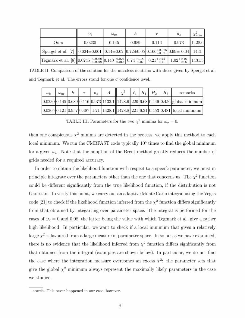
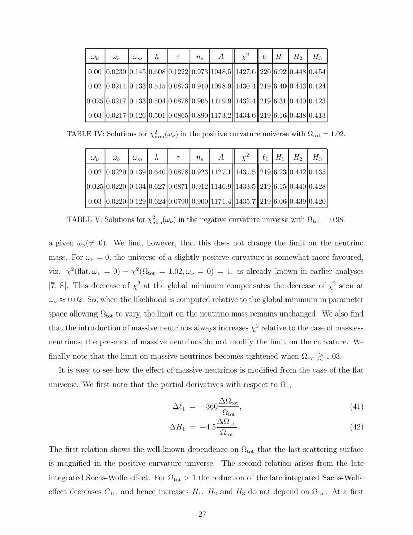
TABLE III: Parameters for the two χ2 minima for ων = 0.

than one conspicuous χ2 minima are detected in the process, we apply this method to each

local minimum. We run the CMBFAST code typically 105 times to find the global minimum

for a given ων . Note that the adoption of the Brent method greatly reduces the number of

grids needed for a required accuracy.

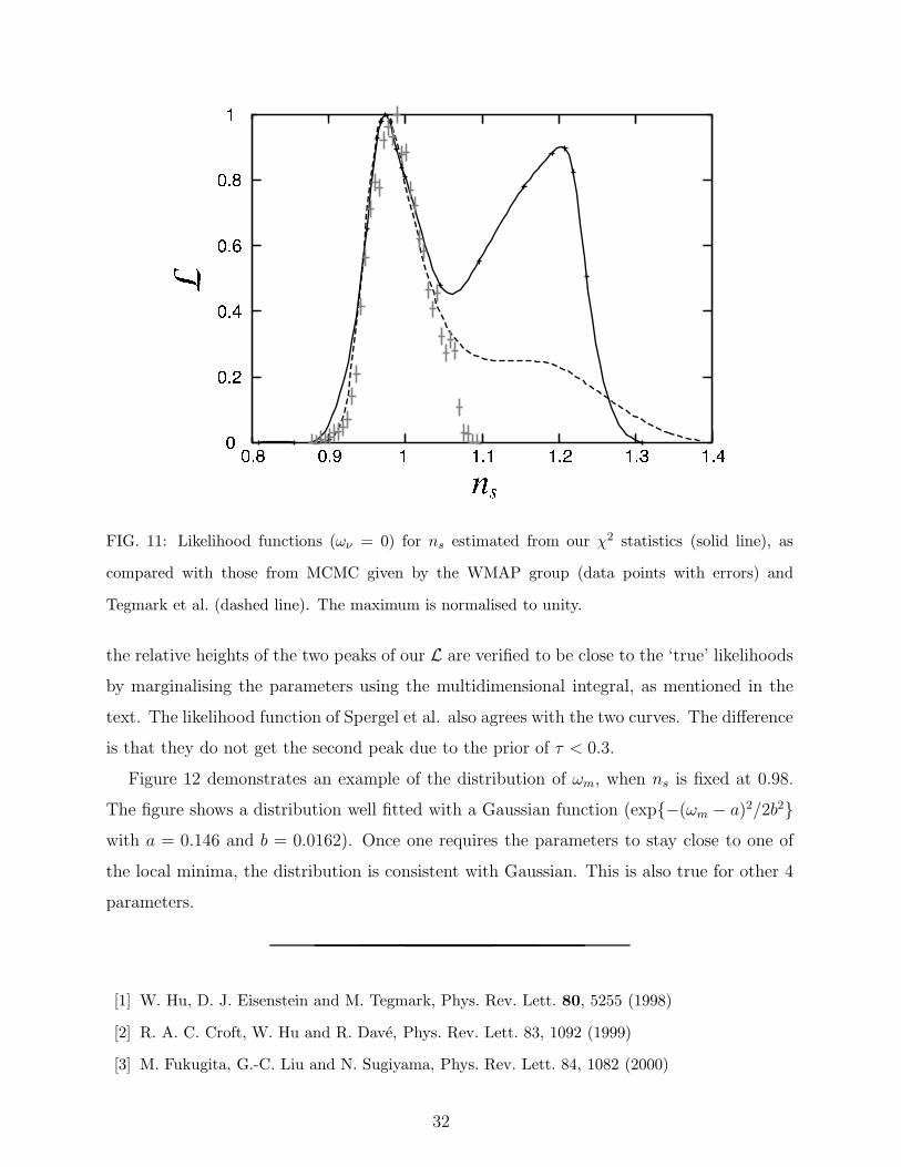
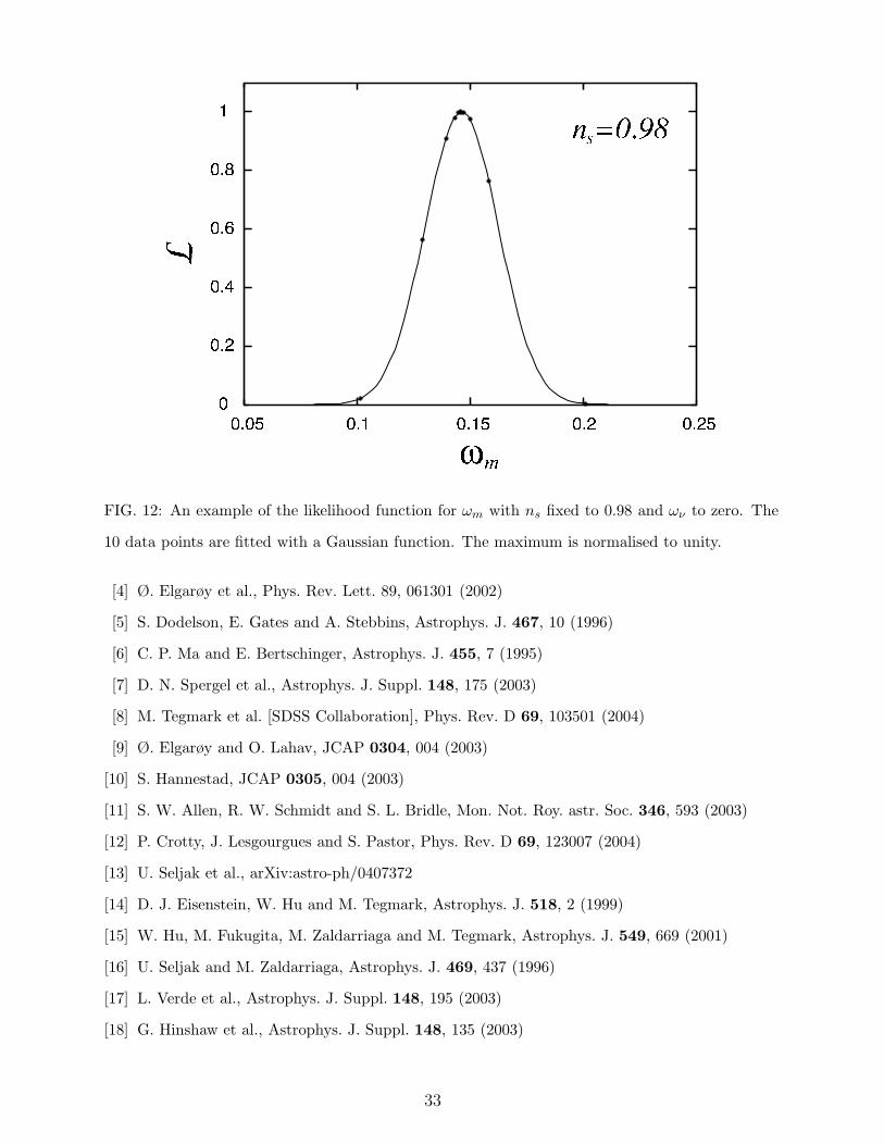
In order to obtain the likelihood function with respect to a specifc parameter, we must in

principle integrate over the parameters other than the one that concerns us. The χ2 function

could be different significantly from the true likelihood function, if the distribution is not

Gaussian. To verify this point, we carry out an adaptive Monte Carlo integral using the Vegas

code [21] to check if the likelihood function inferred from the χ2 function differs significantly

from that obtained by integarting over parameter space. The integral is performed for the

cases of ων = 0 and 0.08, the latter being the value with which Tegmark et al. give a rather

high likelihood. In particular, we want to check if a local minimum that gives a relatively

large χ2 is favoured from a large measure of parameter space. In so far as we have examined,

there is no evidence that the likelihood inferred from χ2 function differs significantly from

that obtained from the integral (examples are shown below). In particular, we do not find

the case where the integration measure overcomes an excess χ2: the parameter sets that

give the global χ2 minimum always represent the maximally likely parameters in the case

we studied.

search. This never happened in our case, however.

8

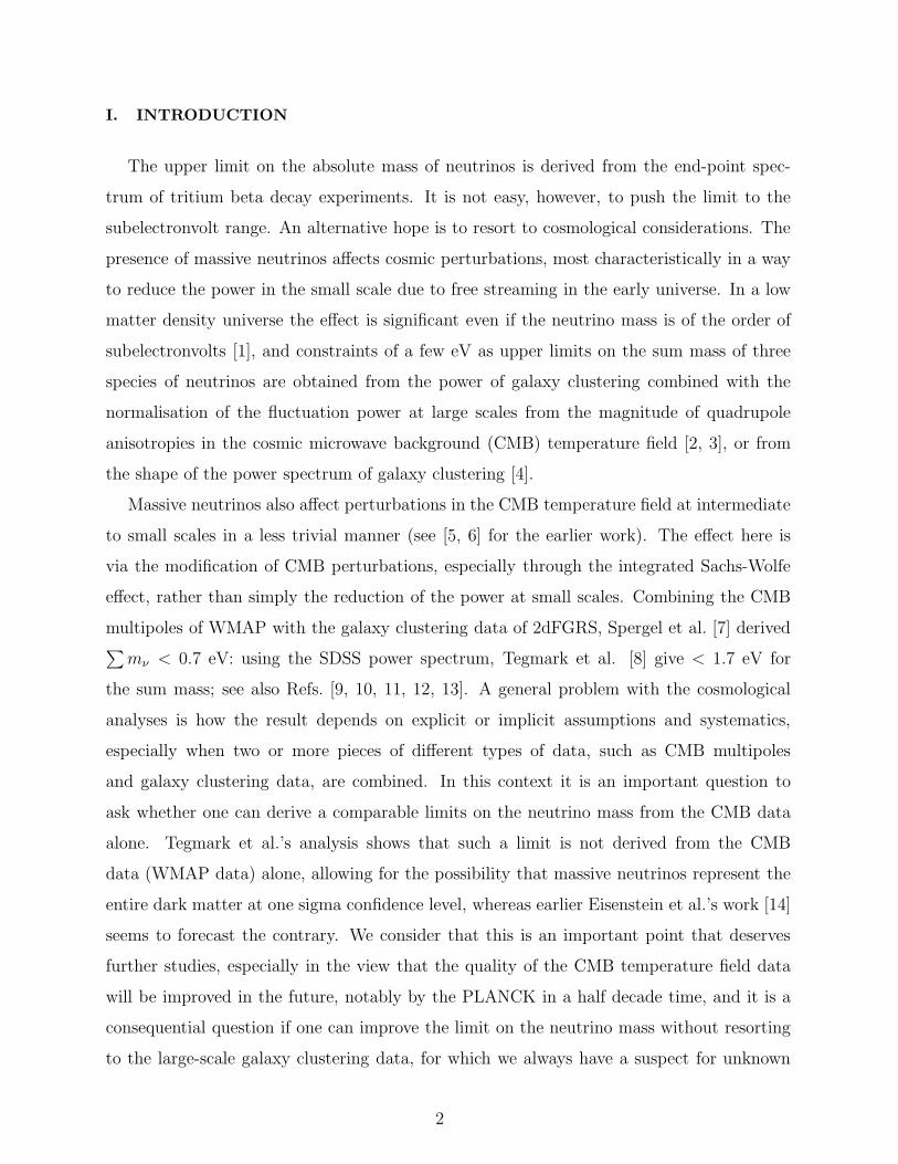
The solutions that give a χ2 minimum for a given ων are presented in Table I. The χ2min

as a function of the neutrino mass density is shown in Figure 1, and the 6 parameters of

the solution for each neutrino mass density, also given in the table, are displayed in Figure

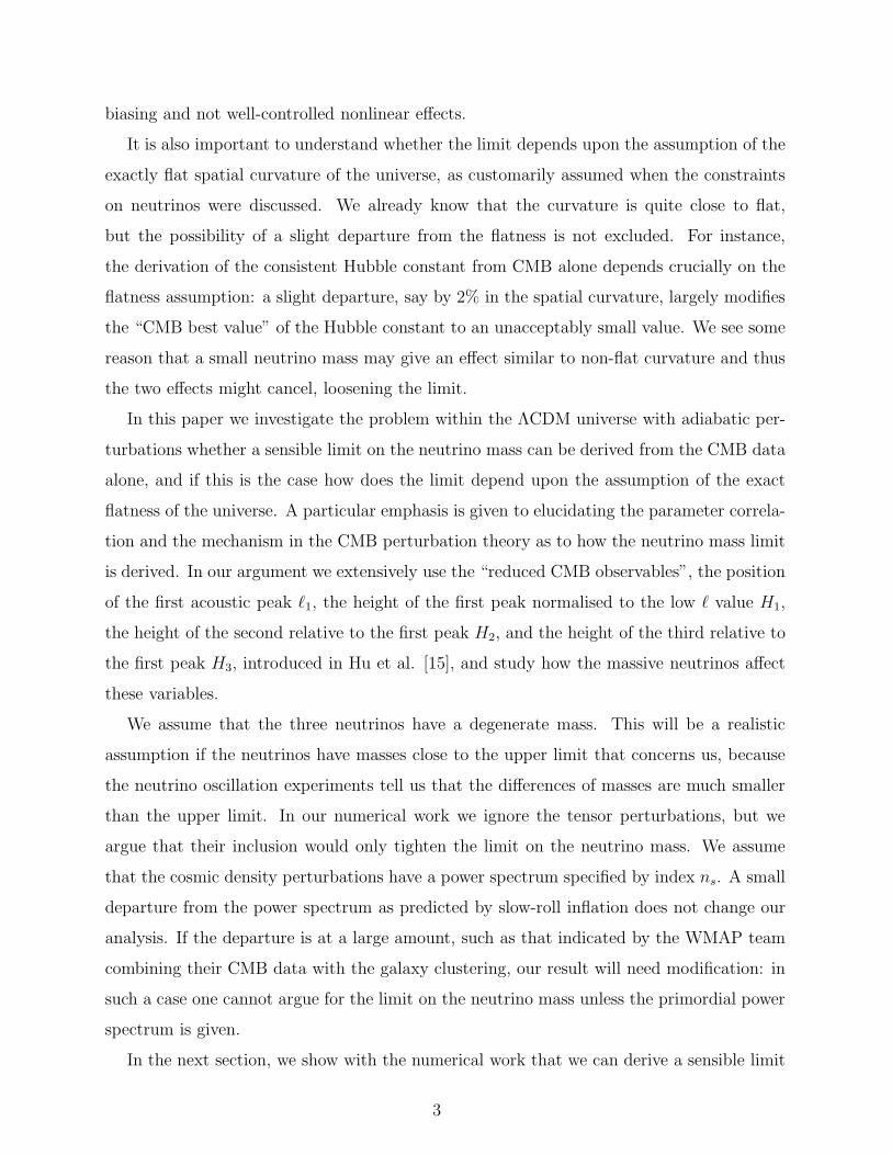
2. The corresponding four reduced CMB observables (defined below) are shown in Figure 3

for the use in the next section.

We first note that the 6 parameters for ων = 0 agree with those of the comparable

solutions of Spergel et al. [7] and Tegmark et al. [8] within one sigma errors (see Table II),

verifying that our minimisation to find the global minimum works at least as good as the

MCMC method they used. In fact, the overall χ2 we attained is appreciably smaller than the

two authors’ for the same set of input data (χ2spergel−χ2

ours = 2.4, and χ2tegmark−χ2

ours = 2.9).

We may ascribe this to a finer grid of the parameters close to the minimum in our work. We

find bimodal structure of the χ2 surface, most clearly visible for ns and τ that are strongly

correlated to each other [8]. The two minima are found at ns = 0.973 and ns = 1.21 with

the second minimum having a slightly larger χ2, χ2(ns = 1.21) − χ2(ns = 0.973) = 0.2, or

the relative likelihood of 1.1: see Table III. The two parameter sets are disjoint by a hill

with a height more than one σ. The Vegas integration over multiparameter space centred

on the two extrema indicates that the former minimum is favoured over the latter by the

ratio of 1.3 in terms of the likelihood value. That is, likelihood from the χ2 estimator is

a good approximation to the ‘true’ value obtained by marginalising the parameters, i.e.,

even in this case where the distribution is deviated from Gaussian the χ2 function is likely

a reasonable approximation of the likelihood function. Furthermore, we observed that the

one-parameter distributions with respect to the other five parameters are close to Gaussian

once we require ns to be around the peak at ns = 0.973 (see Appendix B). This suggests

that the distribution in multidimensional space is likely not far from the Gaussian. Hence,

we infer that the χ2 statistics well approximates the reality.

The bimodal structure we find is consistent with what was found by Tegmark et al.,

but our likelihood of the second minimum is much higher than that reported (the ratio of

likelihoods between the two extrema by Tegmark et al. is 2.5). We suspect that Markov

chain of Tegmark et al. does not sample well around the second minimum. This point is

demonstrated in more detail in Appendix B. This is an example that the current application

of the MCMC does not give an accurate likelihood function away from the global minimum.

Of course, the second solution is an unphysical one in the sense that it is allowed only at

9

the cost of an unacceptably high reionisation optical depth (τ ≈ 0.5); the solution is deleted

with some prior on τ . The resulting parameters ωb, and h are also deviated significantly

from the values derived from other observations.

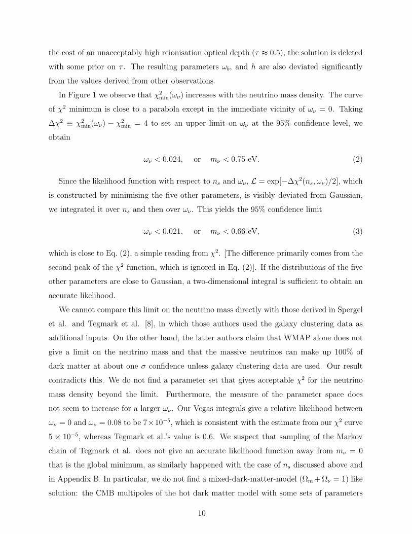
In Figure 1 we observe that χ2min(ων) increases with the neutrino mass density. The curve

of χ2 minimum is close to a parabola except in the immediate vicinity of ων = 0. Taking

∆χ2 ≡ χ2min(ων) − χ2

min = 4 to set an upper limit on ων at the 95% confidence level, we

obtain

ων < 0.024, or mν < 0.75 eV. (2)

Since the likelihood function with respect to ns and ων, L = exp[−∆χ2(ns, ων)/2], which

is constructed by minimising the five other parameters, is visibly deviated from Gaussian,

we integrated it over ns and then over ων . This yields the 95% confidence limit

ων < 0.021, or mν < 0.66 eV, (3)

which is close to Eq. (2), a simple reading from χ2. [The difference primarily comes from the

second peak of the χ2 function, which is ignored in Eq. (2)]. If the distributions of the five

other parameters are close to Gaussian, a two-dimensional integral is sufficient to obtain an

accurate likelihood.

We cannot compare this limit on the neutrino mass directly with those derived in Spergel

et al. and Tegmark et al. [8], in which those authors used the galaxy clustering data as

additional inputs. On the other hand, the latter authors claim that WMAP alone does not

give a limit on the neutrino mass and that the massive neutrinos can make up 100% of

dark matter at about one σ confidence unless galaxy clustering data are used. Our result

contradicts this. We do not find a parameter set that gives acceptable χ2 for the neutrino

mass density beyond the limit. Furthermore, the measure of the parameter space does

not seem to increase for a larger ων . Our Vegas integrals give a relative likelihood between

ων = 0 and ων = 0.08 to be 7×10−5, which is consistent with the estimate from our χ2 curve

5 × 10−5, whereas Tegmark et al.’s value is 0.6. We suspect that sampling of the Markov

chain of Tegmark et al. does not give an accurate likelihood function away from mν = 0

that is the global minimum, as similarly happened with the case of ns discussed above and

in Appendix B. In particular, we do not find a mixed-dark-matter-model (Ωm+Ων = 1) like

solution: the CMB multipoles of the hot dark matter model with some sets of parameters

10

are visibly similar to the observation [9], but a closer inspection shows that χ2 is always

unacceptably large, given a high accuracy of the WMAP data2. In the following section we

see a reason how can one obtain the limit on the neutrino mass density from the CMB data

alone.

We remark that the current WMAP TE data do not seem to play a significant role in

deriving our limit, as we find in separate runs of the χ2 minimisation using only the TT

data3: the χ2 curves differ little between the two cases. This somewhat differs from the

forecast of Eisenstein et al.[14] who indicated a tighter error allowance that would result

with the WMAP polarisation data4.

As a final remark, the two χ2 minima found for ων = 0 persist up to ων ∼ 0.04, but the

one that corresponds to the “unphysical solution” disappears for ων & 0.05.

III. THE REDUCED CMB OBSERVABLES AND THE NEUTRINO MASS

A. The reduced CMB observables and the goodness of the ΛCDM fit

Following Ref. [15], we focus on four quantities which characterise the shape of the CMB

spectrum: the position of the first peak ℓ1, the height of the first peak relative to the large

angular-scale amplitude evaluated at ℓ = 10,

H1 ≡

(

∆Tl1

∆T10

)2

, (4)

the ratio of the second peak height to the first,

H2 ≡

(

∆Tl2

∆Tl1

)2

, (5)

2 For the set of parameters of a mixed-dark-matter-model like solution proposed by Elgarøy & Lahav [9],

we find χ2 = 1482, which is larger than that of the ΛCDM solution by ∆χ2 = 50. We cannot make χ2

significantly smaller around this solution.3 We somewhat loosened the convergence criteria for these runs, but we still obtained χ2

min= 972.3 compared

with 972.4 of Tegmark et al. The solution differs appreciably from that with the full data set only in τ ,

which for the TT case is close to zero.4 Their forecast 2 σ errors are 1.2 eV with the polarisation data, and 1.8 eV without them for a hypothetical

neutrino mass of 0.7 eV assuming idealised CMB data of the Gaussian variance around the prediction of

the ΛCDM model. This does not contradict our actual limit.

11

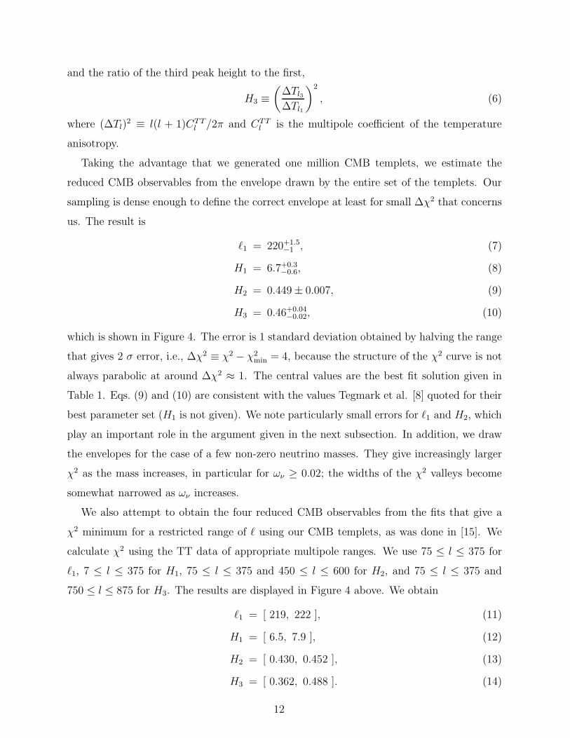
and the ratio of the third peak height to the first,

H3 ≡

(

∆Tl3

∆Tl1

)2

, (6)

where (∆Tl)2 ≡ l(l + 1)CTT

l /2π and CTTl is the multipole coefficient of the temperature

anisotropy.

Taking the advantage that we generated one million CMB templets, we estimate the

reduced CMB observables from the envelope drawn by the entire set of the templets. Our

sampling is dense enough to define the correct envelope at least for small ∆χ2 that concerns

us. The result is

ℓ1 = 220+1.5−1 , (7)

H1 = 6.7+0.3−0.6, (8)

H2 = 0.449± 0.007, (9)

H3 = 0.46+0.04−0.02, (10)

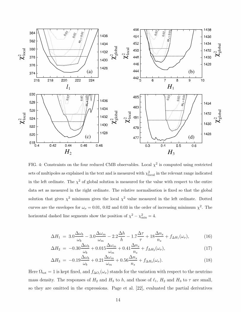
which is shown in Figure 4. The error is 1 standard deviation obtained by halving the range

that gives 2 σ error, i.e., ∆χ2 ≡ χ2 − χ2min = 4, because the structure of the χ2 curve is not

always parabolic at around ∆χ2 ≈ 1. The central values are the best fit solution given in

Table 1. Eqs. (9) and (10) are consistent with the values Tegmark et al. [8] quoted for their

best parameter set (H1 is not given). We note particularly small errors for ℓ1 and H2, which

play an important role in the argument given in the next subsection. In addition, we draw

the envelopes for the case of a few non-zero neutrino masses. They give increasingly larger

χ2 as the mass increases, in particular for ων ≥ 0.02; the widths of the χ2 valleys become

somewhat narrowed as ων increases.

We also attempt to obtain the four reduced CMB observables from the fits that give a

χ2 minimum for a restricted range of ℓ using our CMB templets, as was done in [15]. We

calculate χ2 using the TT data of appropriate multipole ranges. We use 75 ≤ l ≤ 375 for

ℓ1, 7 ≤ l ≤ 375 for H1, 75 ≤ l ≤ 375 and 450 ≤ l ≤ 600 for H2, and 75 ≤ l ≤ 375 and

750 ≤ l ≤ 875 for H3. The results are displayed in Figure 4 above. We obtain

ℓ1 = [ 219, 222 ], (11)

H1 = [ 6.5, 7.9 ], (12)

H2 = [ 0.430, 0.452 ], (13)

H3 = [ 0.362, 0.488 ]. (14)

12

The numbers bracketed are the 1 σ range obtained by halving the 2 σ range of the χ2local

curve5. An inspection of the fits of the templets to the obeserved CMB multipoles indicates

that the data are well represented by those templets. Figure 4 may give the impression that

the χ2 curves do not agree with those obtained from the envelope of the global ΛCDM fit:

the valley of the χ2 curves is generally wider, and the positions of the bottom of valley is

somewhat shifted; the χ2local of the best global fit solution is larger than the best local fits

by ∆χ2 ≈ 2. The central values of Eqs. (7) to (10), however, fall in the one σ range of

Eqs. (11) to (14)6. Our analysis, showing that the best global fit and the local fits resulted

in the consistent reduced CMB parameters within 1 σ, leads us to conclude the goodness of

the ΛCDM fit.

For the consideration given in the next subsection, where we are concerned with the

problem how much massive neutrinos increase χ2 for the CMB data relative to the ων = 0

solution, we should use Eqs. (11) - (14), rather than Eqs. (7) - (10), which are obtained by

restricted parameter searches.

B. Reduced CMB observables and the neutrino mass

We calculate the response of the observables Oi = ℓ1, H1 H2 and H3 with respect to the

variation of cosmological parameters xj , i.e., the partial derivatives ∂Oi/∂xj , around the

global best fit, following Ref. [15]. We vary the parameters typically by ±50% with a step

of 5% and take the difference from the reference values. We find that the responses are

quite linear against the amount of the variations of the 6 parameters. The exception is the

response to the neutrino density parameter, for which it is shown separately. The resulting

partial derivatives are:

∆ℓ1 = 16∆ωb

ωb− 25

∆ωm

ωm− 47

∆h

h+ 36

∆ns

ns+ f∆ℓ1(ων), (15)

5 The 1σ range of H1 depends on the choice of the lower limit of the ℓ-range. It is well known that ℓ = 2 and

3 multipoles are anomalously low compared to the expectation from the ΛCDM model. If the lower limit

is set to ℓmin = 2, the one σ range will be H1 = [7.0, 8.0]. The 1 σ range nearly converges for ℓmin ≥ 3:

the central value does not differ from Eq. (12) more than 0.1.6 The parameters derived by Page et al. [22], who extracted them by fitting the WMAP data by Gaussian

and parabolic functions, ℓ1 = 220.1 ± 0.8, H2 = 0.426 ± 0.015, and H3 = 0.42 ± 0.08 (H1 is not given)

deviate from our ΛCDM solutions in Eqs. (7) to (10) by up to 1.5σ, but agree with those given in Eqs. (11)

to (14).

13

FIG. 4: Constraints on the four reduced CMB observables. Local χ2 is computed using restricted

sets of multipoles as explained in the text and is measured with χ2local in the relevant range indicated

in the left ordinate. The χ2 of global solution is measured for the value with respect to the entire

data set as measured in the right ordinate. The relative normalisation is fixed so that the global

solution that gives χ2 minimum gives the local χ2 value measured in the left ordinate. Dotted

curves are the envelopes for ων = 0.01, 0.02 and 0.03 in the order of increasing minimum χ2. The

horizontal dashed line segments show the position of χ2 − χ2min = 4.

∆H1 = 3.0∆ωb

ωb

− 3.0∆ωm

ωm

− 2.2∆h

h− 1.7

∆τ

τ+ 18

∆ns

ns

+ f∆H1(ων), (16)

∆H2 = −0.30∆ωb

ωb

+ 0.015∆ωm

ωm

+ 0.41∆ns

ns

+ f∆H2(ων), (17)

∆H3 = −0.19∆ωb

ωb

+ 0.21∆ωm

ωm

+ 0.56∆ns

ns

+ f∆H3(ων). (18)

Here Ωtot = 1 is kept fixed, and f∆Oi(ων) stands for the variation with respect to the neutrino

mass density. The responses of H2 and H3 to h, and those of ℓ1, H2 and H3 to τ are small,

so they are omitted in the expressions. Page et al. [22], evaluated the partial derivatives

14

FIG. 5: Response of the four reduced CMB observables to the variation of ων . The isolated points

show the values at ων = 0, which do not connect to the ων 6= 0 values smoothly.

for H2 and H3 to the variations of ωb, ωm and ns for the WMAP data using the analytic

expressions [15]. Our empirical derivatives for these quantities are consistent with their

analytic evaluation.

We draw the response of Oi against the variation of ων for the range ων = 0 to 0.04

in Figures. 5. Note that an increase in ων accompanies a decrease in ΩΛ as we keep

Ωtot = 1 and ωm = ωcdm + ωb fixed7. We see small glitches from ων = 0 to the neighbouring

point in Figures. 5 (b), (c) and (d). This is probably a numerical artefact caused by the

implementation of the massive neutrino subroutine in the CMBFAST code, and we ignore

these glitches since they are much smaller than the errors of the CMB data.

7 Which variables are to be used is merely a matter of the convention. We chose the ones with which the

effect of massive neutrinos is more clearly visible.

15

We observe that the response of the four observables against ων changes at around ων ≈

0.015. As ων increases beyond it, the decrease of ℓ1 becomes gentle; the H1, which increases

with ων up to ων = 0.017, turns to decrease. H2 and H3 change little (< 0.5%) between

ων = 0 and 0.015, but then begin to increase. We can understand this turning point as

the competition between neutrino free streaming and recombination. Neutrinos become

non-relativistic before the recombination when ων & 0.017 and they become non-relativistic

after the recombination when ων . 0.017. We can show that the behaviours, at least for ℓ1

and H1, are quantitatively understood by simple analytical considerations, but let us defer

this problem to the next section.

Here, we are concerned with the problem how the constraint on the neutrino mass is

obtained from the CMB data alone, given observational and empirical information of ℓ1, H1,

H2 and H3. We argue that we cannot derive a constraint for ων < 0.017 but an upper limit

likely exists at some neutrino mass in the region ων & 0.02.

We first consider ων < 0.017. In this regime, as seen in Figure 5, ℓ1 decreases and H1

increases while H2 and H3 change little with increasing ων . The change induced by ων in

ℓ1 is significant, but according to Eq. (15) it is cancelled to a large degree by a decrease of

h [Fig. 2 (c)], as seen in Figure 3 (a). For ων = 0.015, say, we need h to decrease from 0.69

to 0.58, but this change is harmless. The decrease of h, however, causes an increase of H1

(see (16)) in addition to the direct increase due to ων . The increase of H1 is cancelled by

decreases of ns and ωb, whereas those two decreases tend to cancel in H2 and H3. The error

allowance of H1 is large enough that a good cancellation is not required, and hence it is

easy to make the induced changes of H2 and H3 cancelled to within their error allowances.

The large error of H1 arises primarily from the cosmic scatter, σ ∼√

2/(2ℓ+ 1), in small ℓ

modes (which we estimate to give δH1 ≈ ±0.5); so it seems unlikely that it will be reduced

greatly in data expected in the future. Therefore, unless external observational data are

introduced we cannot derive a constraint on the neutrino mass density for ων substantially

smaller than 0.017, consistent with the flat χ2 dependence around ων = 0 in Figure 1. This

will remain to be true even if the quality of the CMB data is improved.

When ων > 0.017, massive neutrinos contribute to increase H2 and H3 as seen in Figures.

5(c) and (d) in addition to a further decrease of ℓ1. Looking at Eq. (17) and Eq. (18), the

increase in H2 and H3 due to massive neutrinos may be compensated by either increasing

ωb or decreasing ns. Actually, as shown in Figure 2 (a) and (e), the decrease of ns occurs

16

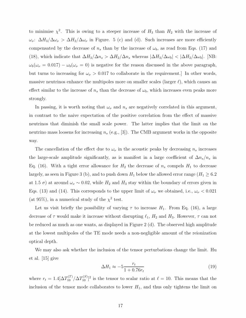
to minimise χ2. This is owing to a steeper increase of H3 than H2 with the increase of

ων : ∆H3/∆ων > ∆H2/∆ων in Figure. 5 (c) and (d). Such increases are more efficiently

compensated by the decrease of ns than by the increase of ωb, as read from Eqs. (17) and

(18), which indicate that ∆H3/∆ns > ∆H2/∆ns whereas |∆H3/∆ωb| < |∆H2/∆ωb|. [NB:

ωb(ων = 0.017) − ωb(ων = 0) is negative for the reason discussed in the above paragraph,

but turns to increasing for ων > 0.017 to collaborate in the requirement.] In other words,

massive neutrinos enhance the multipoles more on smaller scales (larger ℓ), which causes an

effect similar to the increase of ns than the decrease of ωb, which increases even peaks more

strongly.

In passing, it is worth noting that ων and ns are negatively correlated in this argument,

in contrast to the naive expectation of the positive correlation from the effect of massive

neutrinos that diminish the small scale power. The latter implies that the limit on the

neutrino mass loosens for increasing ns (e.g., [3]). The CMB argument works in the opposite

way.

The cancellation of the effect due to ων in the acoustic peaks by decreasing ns increases

the large-scale amplitude significantly, as is manifest in a large coefficient of ∆ns/ns in

Eq. (16). With a tight error allowance for H2 the decrease of ns compels H1 to decrease

largely, as seen in Figure 3 (b), and to push down H1 below the allowed error range (H1 ≥ 6.2

at 1.5 σ) at around ων ∼ 0.02, while H2 and H3 stay within the boundary of errors given in

Eqs. (13) and (14). This corresponds to the upper limit of ων we obtained, i.e., ων < 0.021

(at 95%), in a numerical study of the χ2 test.

Let us visit briefly the possibility of varying τ to increase H1. From Eq. (16), a large

decrease of τ would make it increase without disrupting ℓ1, H2 and H3. However, τ can not

be reduced as much as one wants, as displayed in Figure 2 (d). The observed high amplitude

at the lowest multipoles of the TE mode needs a non-negligible amount of the reionization

optical depth.

We may also ask whether the inclusion of the tensor perturbations change the limit. Hu

et al. [15] give

∆H1 ≈ −5rt

1 + 0.76rt(19)

where rt = 1.4[∆T(T )10 /∆T

(S)10 ]2 is the tensor to scalar ratio at ℓ = 10. This means that the

inclusion of the tensor mode collaborates to lower H1, and thus only tightens the limit on

17

the neutrino mass density.

These considerations show that one can derive the limit on the neutrino mass density

of the order of ων ∼ 0.02 from WMAP data alone. They also show that the limit may be

improved to ων ∼ 0.017 with the use of improved CMB data, but it would not be easy to go

beyond. Even with the extremely high precision data anticipated from PLANCK, the limit

we expect will be ων < 0.013 at the 95% confidence level8: the increase of χ2 is very slow

for ων . 0.019.

The efficient way to improve the limit on ων is to introduce observations that constrain

the Hubble constant, either directly or indirectly, from below. This is because the most

prominent effect caused by light neutrino is to change the position of the first peak and it

is absorbed into a lowering shift of the Hubble constant. Should one require that H0 > 65

km s−1Mpc−1, a significantly stronger limit of the order of ων . 0.01 would be derived even

with the current CMB data10.

IV. ANALYTIC CONSIDERATIONS ON THE EFFECT OF MASSIVE NEUTRI-

NOS

A. The position of the first peak

Here, we attempt to understand the effect of massive neutrinos on the reduced CMB

observables. We may take the epoch when the neutrino of mass mν becomes nonrelativistic

as its momentum pν ∼ mν , i.e., Tν,nr = mν/3. The corresponding redshift is

1 + znr =Tν,nr

Tν,0(20)

= 1.99× 103(mν/eV) (21)

= 6.24× 104ων , (22)

8 In this estimate we use the assumed CMB data that lie around the best ΛCDM solution for the vanishing

neutrino mass with the error being the cosmic variance. We used our data base to search for the χ2

minimum.9 Kaplinghat et al.[23] proposed to use the deflection angle power spectrum from weak gravitational lensing

to give a stronger constraint on mν . We do not take this into accout in the present consideration.10 With this lower limit on H0, the global χ2 minimum is given by the unphysical solution that gives

unreasonably large reionisation optical depth. Our statement in the text excludes this possibility.

18

where∑

mν = 3mν is used for the last equality. This is compared with the redshift at

recombination zrec = 1088 [7], which is insensitive to the mass of neutrinos. Neutrinos

become non-relativistic before recombination, i.e., znr > zrec, if

ων & 0.017, (23)

but otherwise they remain relativistic and freely stream till post recombination epochs.

This ων corresponds approximately to the turning points of the curves of ℓ1, H1, H2 and H3

observed in Figure 5.

We denote the energy density in the form ω ≡ Ωh2 = ρh2/ρcr,0, where the critical density

ρcr,0 = 3MplH20 with the Planck mass defined by the gravity scale M2

pl = 1/8πG, and the

subscript 0 expresses values at the present epoch. The matter and photon energy densities

are

ρm(a)h2/ρcr,0 = ωm,0

(

a

a0

)

−3

, ργ(a)h2/ρcr,0 = ωγ,0

(

a

a0

)

−4

, (24)

where the present photon energy density ωγ,0 = 2.48 × 10−5 for Tγ,0 = 2.725 K [24]. The

neutrino energy density is

ρν(a)h2/ρcr,0 =

45

π4

(

4

11

)4/3

ωγ,0

(

a

a0

)

−4 ∫ ∞

0

√

x2 + y2x2(ex + 1)−1dx, (25)

where

y = mν(11/4)1/3(a/a0)T

−1γ,0 , (26)

and x is the normalised momentum variable and three flavours of neutrinos are assumed to

have a degenerate mass. The vacuum energy is

ρΛ(a)h2/ρcr,0 = ωΛ,0 (27)

= h2 − ωm,0 − ων,0, (28)

for the flat universe. The total energy density is ρtot = ρm + ργ + ρν + ρΛ. With ρtot, the

cosmic expansion rate H = a/a is given by H2 = ρtot/3M2pl, which is used to evaluate the

conformal time η,

η(a) =

∫

dt

a=

∫ a

0

da′

a′2H. (29)

The position of the m-th peak ℓm is determined from that of the acoustic peak ℓA and

the phase shift φm, which depends weakly on m [15],

ℓm = ℓA(m− φm), (30)

19

where the acoustic scale is defined by

ℓA = πrθ(ηrec)

rs(ηrec), (31)

with rs(ηrec) the sound horizon at the recombination epoch and rθ(ηrec) is the comoving

angular diameter distance to the last scattering surface, rθ(ηrec) = η0 − ηrec in the flat

universe. The sound horizon is given by

rs(a) ≡

∫ η(a)

0

csdη =

∫ a

0

cs(a′)

da′

a′2H, (32)

where the sound speed c2s = (1/3)(1 + R)−1 with R = 3ρb/4ργ = 3aωb,0/4ωγ,0. The cs

depends only on photons and baryons, and the effect of neutrino masses enters into the sound

horizon only through the modification of the expansion law. The phase shift in Eq. (30)

arises from the decay of gravitational potential due to radiation growth suppression when

the universe is not fully matter dominated, which later modifies the gravitational redshift

that the photons would otherwise suffer from the Sachs-Wolfe effect [25]. This is sometimes

called the early integrated Sachs-Wolfe effect. The evaluation of the integral gives ℓA ∼ 300,

which is considerably larger than the physical position of ℓ1: the difference is ascribed to

the phase shift φ1, which is estimated in what follows.

The enhancement of the amplitude for scales between the first acoustic peak and the

horizon crossing at the matter domination due to the early integrated Sachs-Wolfe effect

makes the first peak formed at a scale larger than the acoustic peak. An accurate evaluation

of the phase shift φ requires the full solution of the coupled Boltzmann equations. Instead,

we use the fitting formula given in Ref. [15],

φ1 ≈ 0.267(rrec0.3

)0.1

, (33)

where rrec is the radiation-to-matter energy ratio r ≡ ρr/ρm at the recombination. The

appearance of the radiation-to-matter energy ratio as the prime variable is motivated by the

physics of the integrated Sachs-Wolfe effect [25]. Precisely speaking, this fitting formula is

given for massless neutrinos, but it is expected to be valid for massive case provided that rrec

is modified appropriately, because the effect of massive neutrinos on the integrated Sachs-

Wolfe effect is primarily through the change of rrec. A larger radiation-to-matter energy

ratio leads to a larger enhancement and hence a larger phase shift as indicated by Eq. (33).

Massive neutrinos with ων & 0.017 act in a way to suppress this effect.

20

The ratio rrec in the presence of massive neutrinos is calculated as follows. We take

neutrinos that have momentum larger than mν as radiation, and those having smaller mo-

mentum as matter. Accordingly, we split ρν into the radiation component ρν,r and the

matter component ρν,m, as

ρν,r(a)h2/ρcr,0 =

45

π4

(

4

11

)4/3

ωγ,0

(

a

a0

)

−4 ∫ ∞

y

√

x2 + y2x2(ex + 1)−1dx, (34)

ρν,m(a)h2/ρcr,0 =

45

π4

(

4

11

)4/3

ωγ,0

(

a

a0

)

−4 ∫ y

0

√

x2 + y2x2(ex + 1)−1dx, (35)

by dividing the integration range at the value in Eq. (26). The radiation-to-matter energy

ratio is calculated as

ξ = (ργ + ρν,r)/(ρm + ρν,m), (36)

which is used to compute φ1 in Eq. (33).

The first peak position thus calculated as a function of ων is shown in Figure 6 together

with the curve from the full numerical computation presented earlier. The agreement is

excellent, validating the prescription described here. For a reference we also draw the case

where the phase shift is fixed at the zero-neutrino-mass value, (1 − φ1) ∼ 220/300. This

curve agrees with the accurate result for small neutrino masses, but starts deviating from

ων ≈ 0.015, i.e., when neutrinos become nonrelativistic before the recombination epoch.

This stands for the error that we count neutrinos as radiation even when they are non-

relativistic at the recombination, and hence, overestimates the early integrated Sachs-Wolfe

effect, so does the phase shift φ1. This consideration demonstrates that the change of the

slope in ℓ1 at ων ≈ 0.017 is a result of the reduction of the early integrated Sachs-Wolfe

effect by the neutrinos that become nonrelativistic before the recombination epoch.

B. Hights of the acoustic peaks

It is known that free-streaming of massive neutrinos causes a larger decay in the grav-

itational potential Φ. This drives the acoustic oscillation of the baryon-photon fluid more

strongly, so that the amplitude of temperature anisotropies within the free-streaming scale

is enhanced through the monopole term Θ0 + Ψ in the harmonic expansion of the temper-

ature perturbations [5]. The conformal time corresponding to the free-streaming scale is

calculated as ηnr = η(anr) where anr is known from Eq. (22). This is the distance over which

21

FIG. 6: Dependence of ℓ1 on ων calculated from Eq. (30) (dashed line), as compared with the

accurate numerical solution (solid line). The dotted line shows the case when the effect of massive

neutrinos on the early Sachs-Wolfe effect is ignored.

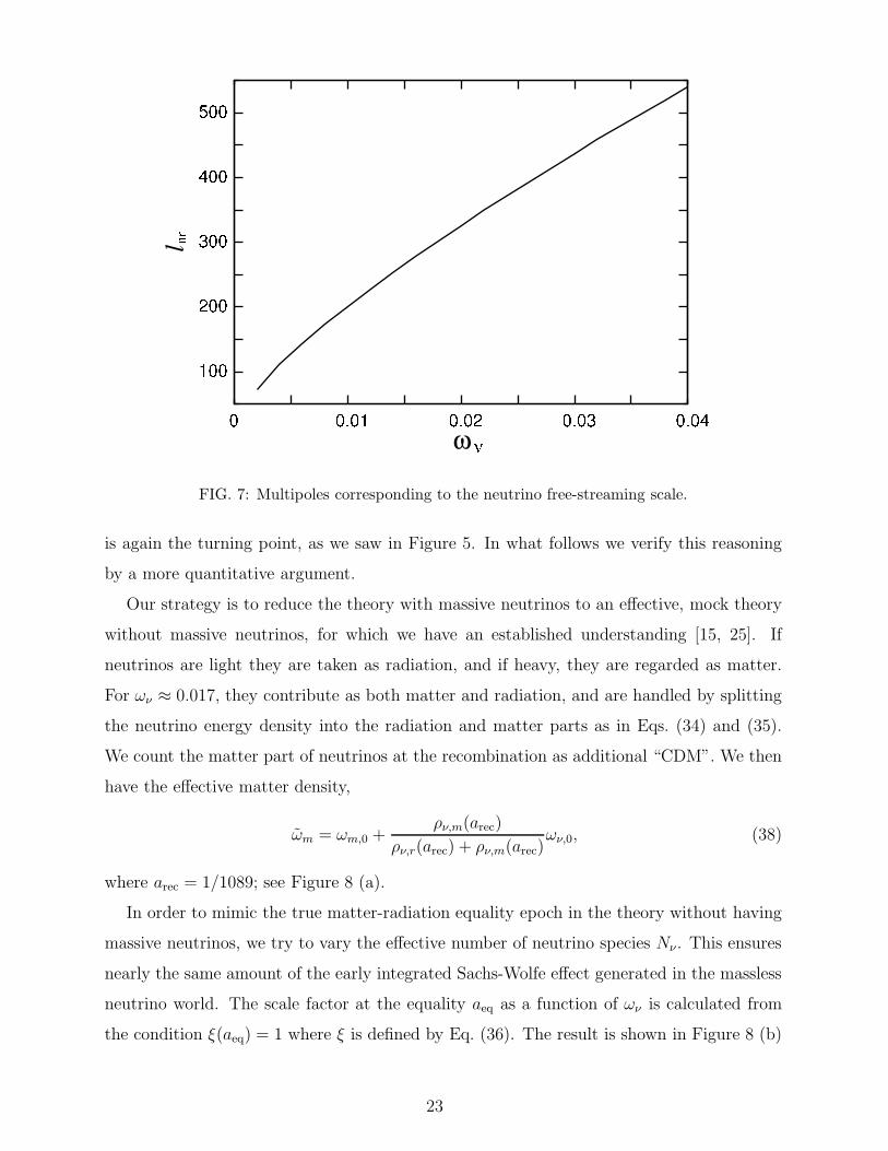
relativistic neutrinos move freely. The multipole ℓnr corresponding to this scale is [25]:

ℓnr ≃2πrθ(ηrec)

ηnr, (37)

which we show in Figure 7 for ωm,0 = 0.14 and h = 0.69, and zrec = 1088. The multipole

amplitudes for ℓ > ℓnr are affected by free streaming. For ων > 0.017, the amplitude on the

scale ℓ > 300 is enhanced [5]. This means that only the second and higher peaks receive the

effect.

The first peak receives little the effect of the decay of gravitational potential, and the

variation of H1 with ων is understood by a simple consideration. The gentle increase of

H1 for ων . 0.017 is understood by the decrease of ΩΛ to compensate the neutrino energy

density in the flat universe and an associated decrease of the integrated Sachs-Wolfe effect

from the late domination of Λ, which enhances C10. The effect continues to the region

ων & 0.017, but in this regime massive neutrinos act as the nonrelativistic dark matter at

recombination and the effect from the increase of the amount of matter overcomes; hence

H1 begins to decrease [∆H1/∆ωm < 0 as seen in Eq. (16)]. This indicates that ων ∼ 0.017

22

FIG. 7: Multipoles corresponding to the neutrino free-streaming scale.

is again the turning point, as we saw in Figure 5. In what follows we verify this reasoning

by a more quantitative argument.

Our strategy is to reduce the theory with massive neutrinos to an effective, mock theory

without massive neutrinos, for which we have an established understanding [15, 25]. If

neutrinos are light they are taken as radiation, and if heavy, they are regarded as matter.

For ων ≈ 0.017, they contribute as both matter and radiation, and are handled by splitting

the neutrino energy density into the radiation and matter parts as in Eqs. (34) and (35).

We count the matter part of neutrinos at the recombination as additional “CDM”. We then

have the effective matter density,

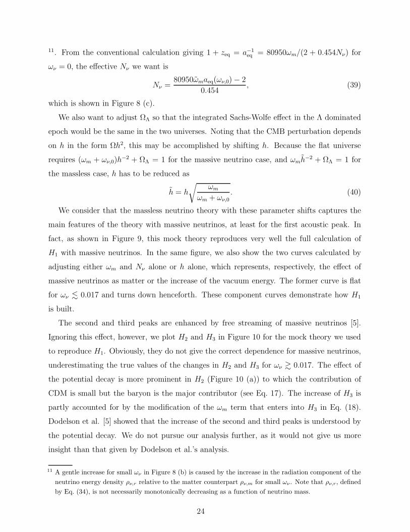
ωm = ωm,0 +ρν,m(arec)

ρν,r(arec) + ρν,m(arec)ων,0, (38)

where arec = 1/1089; see Figure 8 (a).

In order to mimic the true matter-radiation equality epoch in the theory without having

massive neutrinos, we try to vary the effective number of neutrino species Nν . This ensures

nearly the same amount of the early integrated Sachs-Wolfe effect generated in the massless

neutrino world. The scale factor at the equality aeq as a function of ων is calculated from

the condition ξ(aeq) = 1 where ξ is defined by Eq. (36). The result is shown in Figure 8 (b)

23

11. From the conventional calculation giving 1 + zeq = a−1eq = 80950ωm/(2 + 0.454Nν) for

ων = 0, the effective Nν we want is

Nν =80950ωmaeq(ων,0)− 2

0.454, (39)

which is shown in Figure 8 (c).

We also want to adjust ΩΛ so that the integrated Sachs-Wolfe effect in the Λ dominated

epoch would be the same in the two universes. Noting that the CMB perturbation depends

on h in the form Ωh2, this may be accomplished by shifting h. Because the flat universe

requires (ωm + ων,0)h−2 + ΩΛ = 1 for the massive neutrino case, and ωmh

−2 + ΩΛ = 1 for

the massless case, h has to be reduced as

h = h

√

ωm

ωm + ων,0. (40)

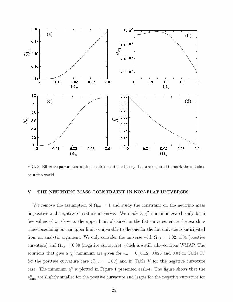
We consider that the massless neutrino theory with these parameter shifts captures the

main features of the theory with massive neutrinos, at least for the first acoustic peak. In

fact, as shown in Figure 9, this mock theory reproduces very well the full calculation of

H1 with massive neutrinos. In the same figure, we also show the two curves calculated by

adjusting either ωm and Nν alone or h alone, which represents, respectively, the effect of

massive neutrinos as matter or the increase of the vacuum energy. The former curve is flat

for ων . 0.017 and turns down henceforth. These component curves demonstrate how H1

is built.

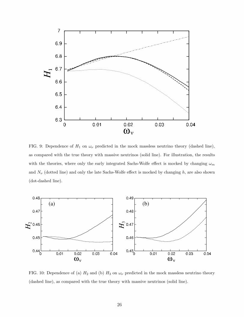
The second and third peaks are enhanced by free streaming of massive neutrinos [5].

Ignoring this effect, however, we plot H2 and H3 in Figure 10 for the mock theory we used

to reproduce H1. Obviously, they do not give the correct dependence for massive neutrinos,

underestimating the true values of the changes in H2 and H3 for ων & 0.017. The effect of

the potential decay is more prominent in H2 (Figure 10 (a)) to which the contribution of

CDM is small but the baryon is the major contributor (see Eq. 17). The increase of H3 is

partly accounted for by the modification of the ωm term that enters into H3 in Eq. (18).

Dodelson et al. [5] showed that the increase of the second and third peaks is understood by

the potential decay. We do not pursue our analysis further, as it would not give us more

insight than that given by Dodelson et al.’s analysis.

11 A gentle increase for small ων in Figure 8 (b) is caused by the increase in the radiation component of the

neutrino energy density ρν,r relative to the matter counterpart ρν,m for small ων . Note that ρν,r, defined

by Eq. (34), is not necessarily monotonically decreasing as a function of neutrino mass.

24

FIG. 8: Effective parameters of the massless neutrino theory that are required to mock the massless

neutrino world.

V. THE NEUTRINO MASS CONSTRAINT IN NON-FLAT UNIVERSES

We remove the assumption of Ωtot = 1 and study the constraint on the neutrino mass

in positive and negative curvature universes. We made a χ2 minimum search only for a

few values of ων close to the upper limit obtained in the flat universe, since the search is

time-consuming but an upper limit comparable to the one for the flat universe is anticipated

from an analytic argument. We only consider the universe with Ωtot = 1.02, 1.04 (positive

curvature) and Ωtot = 0.98 (negative curvature), which are still allowed from WMAP. The

solutions that give a χ2 minimum are given for ων = 0, 0.02, 0.025 and 0.03 in Table IV

for the positive curvature case (Ωtot = 1.02) and in Table V for the negative curvature

case. The minimum χ2 is plotted in Figure 1 presented earlier. The figure shows that the

χ2min are slightly smaller for the positive curvature and larger for the negative curvature for

25

FIG. 9: Dependence of H1 on ων predicted in the mock massless neutrino theory (dashed line),

as compared with the true theory with massive neutrinos (solid line). For illustration, the results

with the theories, where only the early integrated Sachs-Wolfe effect is mocked by changing ωm

and Nν (dotted line) and only the late Sachs-Wolfe effect is mocked by changing h, are also shown

(dot-dashed line).

FIG. 10: Dependence of (a) H2 and (b) H3 on ων predicted in the mock massless neutrino theory

(dashed line), as compared with the true theory with massive neutrinos (solid line).

26

ων ωb ωm h τ ns A χ2 ℓ1 H1 H2 H3

0.00 0.0230 0.145 0.608 0.1222 0.973 1048.5 1427.6 220 6.92 0.448 0.454

0.02 0.0214 0.133 0.515 0.0873 0.910 1098.9 1430.4 219 6.40 0.443 0.424

0.025 0.0217 0.133 0.504 0.0878 0.905 1119.9 1432.4 219 6.31 0.440 0.423

0.03 0.0217 0.126 0.501 0.0865 0.890 1173.2 1434.6 219 6.16 0.438 0.413

TABLE IV: Solutions for χ2min(ων) in the positive curvature universe with Ωtot = 1.02.

ων ωb ωm h τ ns A χ2 ℓ1 H1 H2 H3

0.02 0.0220 0.139 0.640 0.0878 0.923 1127.1 1431.5 219 6.23 0.442 0.435

0.025 0.0220 0.134 0.627 0.0871 0.912 1146.9 1433.5 219 6.15 0.440 0.428

0.03 0.0220 0.129 0.624 0.0790 0.900 1171.4 1435.7 219 6.06 0.439 0.420

TABLE V: Solutions for χ2min(ων) in the negative curvature universe with Ωtot = 0.98.

a given ων( 6= 0). We find, however, that this does not change the limit on the neutrino

mass. For ων = 0, the universe of a slightly positive curvature is somewhat more favoured,

viz. χ2(flat, ων = 0) − χ2(Ωtot = 1.02, ων = 0) = 1, as already known in earlier analyses

[7, 8]. This decrease of χ2 at the global minimum compensates the decrease of χ2 seen at

ων ≈ 0.02. So, when the likelihood is computed relative to the global minimum in parameter

space allowing Ωtot to vary, the limit on the neutrino mass remains unchanged. We also find

that the introduction of massive neutrinos always increases χ2 relative to the case of massless

neutrinos; the presence of massive neutrinos do not modify the limit on the curvature. We

finally note that the limit on massive neutrinos becomes tightened when Ωtot & 1.03.

It is easy to see how the effect of massive neutrinos is modified from the case of the flat

universe. We first note that the partial derivatives with respect to Ωtot

∆ℓ1 = −360∆Ωtot

Ωtot

, (41)

∆H1 = +4.5∆Ωtot

Ωtot

. (42)

The first relation shows the well-known dependence on Ωtot that the last scattering surface

is magnified in the positive curvature universe. The second relation arises from the late

integrated Sachs-Wolfe effect. For Ωtot > 1 the reduction of the late integrated Sachs-Wolfe

effect decreases C10, and hence increases H1. H2 and H3 do not depend on Ωtot. At a first

27

glance one might suspect that a large response of ℓ1 to Ωtot for Ωtot < 1 would cancel the

negative change of ℓ1 induced by a finite neutrino mass and relax the limit for the negative

curvature universe. This, however, is not the case.

The position of ℓ1 is tightly constrained by the data. So the change in ℓ1 from either

the massive neutrino or the departure from the flat space curvature is compensated by the

change in h that is unconstrained. The negative curvature makes this shift smaller, and

the positive makes it larger as seen in Figure 2 (c). Note that among the 6 cosmological

parameters, only h receives a significant change when a small curvature is introduced. All

other parameters change no more than a few percent from the values for the flat universe.

The positive curvature increases H1 via Eq. (42) and an extra decrease of h also increases

H1. The increase of H1 makes some more allowance to the observational lower limit of H1,

which lowers χ2 and would in principle weakens the constraint. However, when we remove

the spatial flatness assumption, the global χ2 minimum, realised at ων = 0, occurs at a χ2

smaller than that for the flat universe. This offsets the decrease of χ2(ων 6= 0), and we obtain

the limit on the neutrino mass virtually unchanged from the case for the flat universe.

Although the limit on the neutrino mass is formally unchanged in a positive curvature

universe, the cost is a significant decrease of h as seen in Figure 2 (c). To realise the 2 σ

limit, ων ∼ 0.021, we are led to H0 ≈ 50 km s−1Mpc−1, an unacceptably small value.

The argument may go in the opposite way for the negative curvature, but the limit on the

neutrino mass becomes substantially stronger. We calculate ∆χ2 in a full non-zero curvature

parameter space: for negative curvatures ∆χ2(ων = 0) is already significant relative to the

global minimum that is realised in a positive curvature universe.

Note that our discussion does not deal with H2 and H3, because these quantities depend

on neither Ωtot or h directly. The change of these quantities takes place only through the

adjustment of other parameters, and is small.

In conclusion we find that the constraint on the neutrino mass we obtained for the flat

universe ων < 0.021 is unchanged even when a non-zero spatial curvature is allowed.

VI. CONCLUSION

We showed that the subelectronvolt upper limit can be derived on the neutrino mass

from the CMB data alone within the ΛCDM model with adiabatic perturbations. This

28

is contrary to the statements made in Elgarøy and Lahav [9] and Tegmark et al.[8], who

stressed that the large-scale galaxy clustering information is essential to derive the limit

on the neutrino mass. Assuming the flatness of the universe, the constraint we obtained

from the one-year data of the WMAP observation alone by maximising the likelihood is

ων < 0.021 or∑

mν < 2.0 eV at the 95% confidence level (for the degenerate neutrinos,

which are close to the reality if the neutrino mass is close to the limit, mν < 0.66 eV). This

is slightly weaker than the limit < 1.7 eV [8] derived by the combined use of WMAP and

SDSS data, or similar limits that are obtained by combining more different types of data

[7, 9, 10, 11, 12, 13], but our limit is a robust result in the sense that it does not receive any

systematics from biasing, non-linear effects and others, and solely determined by the CMB

data for which systematics are controlled very well. Our constraint is unchanged even if we

relax the flatness assumption. The inclusion of the tensor perturbation only tightens the

limit. The assumption we still need is the power-law primordial fluctuation spectrum.

We argued that it would not be easy to improve the limit beyond∑

mν . 1.5 eV using the

CMB data alone, even if the CMB multipole data are substantially improved. This “critical

limit” corresponds to the situation when neutrino becomes nonrelativistic at recombination

epoch. That is, we can derive the constraint when neutrinos become nonrelativistic before

the recombination epoch. The improvement of the limit on the neutrino mass requires some

external inputs, most characteristically the lower limit on the Hubble constant, or those that

effectively leads to the constraint on the Hubble constant, such as the Type Ia supernova

Hubble diagram or the large-scale clustering of galaxies. If H0 would receives a firm lower

limit, say H0 > 65 km s−1Mpc−1, the upper limit on the neutrino mass would be tightened

to∑

mν < 0.8 eV.

We demonstrated the mechanism as to how these constraints are derived, using the re-

duced CMB observables, ℓ1, H1, H2 and H3 introduced by [15], and studying their responses

to the neutrino mass density. The key point is that ℓ1 and H2 are constrained to narrow

ranges by observation, and the variation of the cosmological parameters induced by the finite

neutrino density cannot be accommodated in the error budget of H1 with the increase of

the neutrino mass beyond∑

mν ∼ 2 eV.

We also showed that the response of the reduced CMB observables, in particular ℓ1 and

H1, to the neutrino mass density is understood by the modification of the integrated Sachs-

Wolfe effect in the presence of massive neutrinos. In addition, free streaming of massive

29

neutrinos promotes the decay of gravitational potential that enhances H2 and H3, whose

scales are within free streaming [5]. This leads to the negative correlation between ns and

mν , in contrast to the positive correlation expected from the suppression of the small scale

power due to massive neutrinos.

The most important message from our analysis is that (i) one can derive the upper limit

on the neutrino mass, which is only slightly weaker than is quoted in the modern literature,

using the CMB (WMAP) data alone: hereby, one can avoid to make use of the mixed data

of different quality or with possible systematic effects such as biasing and nonlinear effects

for galaxies, and (ii) one may improve the limit by a modest amount even when the quality

of the CMB data is improved, but not much. For a substantial improvement of the limit

one needs a constraint on the Hubble constant from below.

APPENDIX A: MULTIDIMENSIONAL χ2-MINIMIZATION

Our problem is to minimise f = χ2(ns, ωm, ωb, τ, h, A) in 6-dimensional parameter space.

Since we want to avoid to calculate the derivative, we adopt the Brent method [20] and

generalise it to a multidimensional problem. For one dimensional problem the Brent method

samples 3 points, f(xa), f(xc), f(xb), and draw a parabola that connects the three f ’s to

find the value x1 that give the valley of f . Then f(x1) and the two neighbouring f ’s are

used to find the next parabola and its valley at x2. This process is successively applied until

desired convergence.

For multidimensional problem, say, f(x, y, z), we first minimise f with respect to z, by

applying the Brent method in this direction, with x and y fixed to an arbitrary grid xa

and ya. We find successively new z grids z1(xa, ya), z2(xa, ya), ..., and eventually reach

f(xa, ya, zmin(xa, ya)). We next minimise it with respect to y using (ya, yb, yc). We carry out

the z minimisation for yb and yc, i.e., f(xa, yb, zmin(xa, yb)) and f(xa, yc, zmin(xa, yc)), and

successively adding a new y grid, y1, y2..., while repeating the z minimisation procedure at

each step; we eventually arrive at f(xa, ymin(xa), zmin(xa, ymin(xa))). We repeat the same

procedure with respect to x. Starting from

f(xa, ymin(xa), zmin(xa, ymin(xa))),

f(xb, ymin(xb), zmin(xb, ymin(xb))),

30

f(xc, ymin(xc), zmin(xc, ymin(xc))),

we finally find

f(xmin, ymin(xmin), zmin(xmin, ymin(xmin))),

which is the desired result.

For our problem of f = χ2(ns, ωm, ωb, τ, h, A), applying the minimisation in the order

of A, h, τ, ωb, ωm and ns, the final value would be χ2(ns,min, ωm,min, ωb,min, τmin, hmin, Amin),

where the omitted arguments are

ωm,min = ωm,min(ns,min), (A1)

ωb,min = ωb,min(ns,min, ωm,min), (A2)

τmin = τmin(ns,min, ωm,min, ωb,min), (A3)

hmin = hmin(ns,min, ωm,min, ωb,min, τmin), (A4)

Amin = Amin(ns,min, ωm,min, ωb,min, τmin, hmin). (A5)

We find that this nested one-dimensional minimizations works well for the WMAP χ2

function and the minimum obtained gives χ2 lower than those found by the Markov chain

Monte Carlo methods given in the literature. A caution is needed for the outermost nest,

the minimization with respect to ns. We find two minima for a small ων . So we apply

the minimisation procedure for each case separately. If more than one mininum is found

in the course of intermediate minimisation, we must divide the parameter space and the

minimisation procedure must be applied separately. We do not find, however, such cases

other than that quoted above.

APPENDIX B: COMPARISON OF THE GRID SEARCH AND MCMC

We compare the likelihood function for ων = 0 inferred from the χ2 function with those

obtained by the MCMC given in the literature. In Figure 11 we present L = exp(−∆χ2/2)

and L given by Tegmark et al. [8] and Spergel et al. [7] for the variable ns. We see that

our likelihood function agrees very well with Tegmark et al.’s for ns < 1.05, but it starts

deviating for ns > 1.05, where our likelihood function is much larger, meaning that Tegmark

et al.’s chain does not find a true local minimum near the second peak. We emphasise that

31

FIG. 11: Likelihood functions (ων = 0) for ns estimated from our χ2 statistics (solid line), as

compared with those from MCMC given by the WMAP group (data points with errors) and

Tegmark et al. (dashed line). The maximum is normalised to unity.

the relative heights of the two peaks of our L are verified to be close to the ‘true’ likelihoods

by marginalising the parameters using the multidimensional integral, as mentioned in the

text. The likelihood function of Spergel et al. also agrees with the two curves. The difference

is that they do not get the second peak due to the prior of τ < 0.3.

Figure 12 demonstrates an example of the distribution of ωm, when ns is fixed at 0.98.

The figure shows a distribution well fitted with a Gaussian function (exp−(ωm − a)2/2b2

with a = 0.146 and b = 0.0162). Once one requires the parameters to stay close to one of

the local minima, the distribution is consistent with Gaussian. This is also true for other 4

parameters.

[1] W. Hu, D. J. Eisenstein and M. Tegmark, Phys. Rev. Lett. 80, 5255 (1998)

[2] R. A. C. Croft, W. Hu and R. Dave, Phys. Rev. Lett. 83, 1092 (1999)

[3] M. Fukugita, G.-C. Liu and N. Sugiyama, Phys. Rev. Lett. 84, 1082 (2000)

32

FIG. 12: An example of the likelihood function for ωm with ns fixed to 0.98 and ων to zero. The

10 data points are fitted with a Gaussian function. The maximum is normalised to unity.

[4] Ø. Elgarøy et al., Phys. Rev. Lett. 89, 061301 (2002)

[5] S. Dodelson, E. Gates and A. Stebbins, Astrophys. J. 467, 10 (1996)

[6] C. P. Ma and E. Bertschinger, Astrophys. J. 455, 7 (1995)

[7] D. N. Spergel et al., Astrophys. J. Suppl. 148, 175 (2003)

[8] M. Tegmark et al. [SDSS Collaboration], Phys. Rev. D 69, 103501 (2004)

[9] Ø. Elgarøy and O. Lahav, JCAP 0304, 004 (2003)

[10] S. Hannestad, JCAP 0305, 004 (2003)

[11] S. W. Allen, R. W. Schmidt and S. L. Bridle, Mon. Not. Roy. astr. Soc. 346, 593 (2003)

[12] P. Crotty, J. Lesgourgues and S. Pastor, Phys. Rev. D 69, 123007 (2004)

[13] U. Seljak et al., arXiv:astro-ph/0407372

[14] D. J. Eisenstein, W. Hu and M. Tegmark, Astrophys. J. 518, 2 (1999)

[15] W. Hu, M. Fukugita, M. Zaldarriaga and M. Tegmark, Astrophys. J. 549, 669 (2001)

[16] U. Seljak and M. Zaldarriaga, Astrophys. J. 469, 437 (1996)

[17] L. Verde et al., Astrophys. J. Suppl. 148, 195 (2003)

[18] G. Hinshaw et al., Astrophys. J. Suppl. 148, 135 (2003)

33

[19] A. Kogut et al., Astrophys. J. Suppl. 148, 161 (2003)

[20] R. P. Brent, Algorithms for Minimization without Derivatives (Prentice-Hall, Englewood Clifs,

NJ, U.S.A. 1973); see also W. H. Press, B. P. Flannery, S. A. Teukolsky and W. T. Vetterling,

Numerical Recipes (Cambridge University Press, New York, 1986)

[21] G. P. Lepage, J. Comput. Phys. 27, 192 (1978)

[22] L. Page et al., Astrophys. J. Suppl. 148, 233 (2003)

[23] M. Kaplinghat, L. Knox and Y. S. Song, Phys. Rev. Lett. 91, 241301 (2003)

[24] J. C. Mather, D. J. Fixsen, R. A. Shafer, C. Mosier and D. T. Wilkinson, Astrophys. J. 512,

511 (1999)

[25] W. Hu and N. Sugiyama, Phys. Rev. D 51, 2599 (1995)

34