Constraints in Graph Drawing...

Constraints, An International Journal, 3, 87–120 (1998)c© 1998 Kluwer Academic Publishers, Boston. Manufactured in The Netherlands.

Constraints in Graph Drawing Algorithms

ROBERTO TAMASSIA [email protected] of Computer Science, Brown University, Providence, RI 02912–1910, USA

Abstract. Graphs are widely used for information visualization purposes, since they provide a natural and intuitiverepresentation of complex abstract structures. The automatic generation of drawings of graphs has applicationsa variety of fields such as software engineering, database systems, and graphical user interfaces. In this paper,we survey algorithmic techniques for graph drawing that support the expression and satisfaction of user-definedconstraints.

1. Introduction

Graph drawing addresses the problem of constructing geometric representations of graphs,and is a major aspect of the emerging field of information visualization. Graph drawing hasapplications to key computer technologies such as software engineering, database systems,information retrieval, visual interfaces, and computer-aided-design. Research on graphdrawing has been conducted within several diverse areas, including discrete mathematics(topological graph theory, geometric graph theory, order theory), algorithmics (graph al-gorithms, data structures, computational geometry,VLSI), and human-computer interaction(visual languages, graphical user interfaces, software visualization).

There are infinitely many drawings for a graph. A drawingconventiondictates basic rulesfor mapping vertices and edges to geometric objects. Commonly used drawing conventionsinclude:

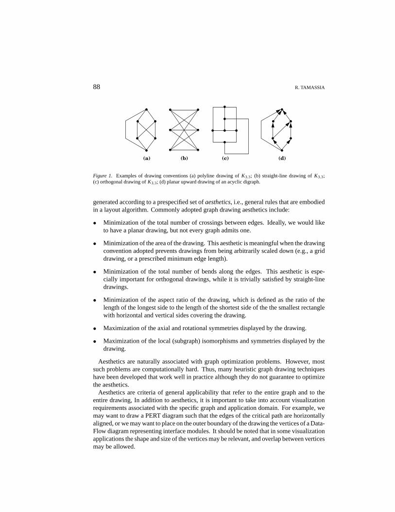
Polyline drawing: each edge is drawn as a polygonal chain (Fig. 1.a).

Straight-line drawing: each edge is drawn as a straight line segment (Fig. 1.b).

Orthogonal drawing: each edge is drawn as a polygonal chain of alternating horizontaland vertical segments (Fig. 1.c).

Grid drawing: vertices, crossings, and edge bends have integer coordinates.

Upward (downward) drawing:(for directed acyclic graphs) each edge is drawn monoton-ically increasing (decreasing) in the vertical direction (Fig. 1.d).

In order to effectively draw a graph, we would like to take into account a variety ofproperties. For example, planarity and the display of symmetries are highly desirable invisualization applications. Also, it is customary to display trees and acyclic digraphs withupward drawings. In general, to avoid wasting valuable space on a page or a computerscreen, it is important to keep the area of the drawing small. Drawing a graph can thusbe formalized as a multi-objective optimization problem, where the layout of the graph is

88 R. TAMASSIA

(a) (b) (c) (d)

Figure 1. Examples of drawing conventions (a) polyline drawing ofK3,3; (b) straight-line drawing ofK3,3;(c) orthogonal drawing ofK3,3; (d) planar upward drawing of an acyclic digraph.

generated according to a prespecified set ofaesthetics, i.e., general rules that are embodiedin a layout algorithm. Commonly adopted graph drawing aesthetics include:

• Minimization of the total number of crossings between edges. Ideally, we would liketo have a planar drawing, but not every graph admits one.

• Minimization of the area of the drawing. This aesthetic is meaningful when the drawingconvention adopted prevents drawings from being arbitrarily scaled down (e.g., a griddrawing, or a prescribed minimum edge length).

• Minimization of the total number of bends along the edges. This aesthetic is espe-cially important for orthogonal drawings, while it is trivially satisfied by straight-linedrawings.

• Minimization of the aspect ratio of the drawing, which is defined as the ratio of thelength of the longest side to the length of the shortest side of the the smallest rectanglewith horizontal and vertical sides covering the drawing.

• Maximization of the axial and rotational symmetries displayed by the drawing.

• Maximization of the local (subgraph) isomorphisms and symmetries displayed by thedrawing.

Aesthetics are naturally associated with graph optimization problems. However, mostsuch problems are computationally hard. Thus, many heuristic graph drawing techniqueshave been developed that work well in practice although they do not guarantee to optimizethe aesthetics.

Aesthetics are criteria of general applicability that refer to the entire graph and to theentire drawing, In addition to aesthetics, it is important to take into account visualizationrequirements associated with the specific graph and application domain. For example, wemay want to draw a PERT diagram such that the edges of the critical path are horizontallyaligned, or we may want to place on the outer boundary of the drawing the vertices of a Data-Flow diagram representing interface modules. It should be noted that in some visualizationapplications the shape and size of the vertices may be relevant, and overlap between verticesmay be allowed.

CONSTRAINTS IN GRAPH DRAWING ALGORITHMS 89

These specific requirements can be viewed asconstraintsand should be considered asadditional input to the drawing problem. Widely used graph drawing constraints include:

• Place a given vertex in the “center” of the drawing.

• Place a given vertex on the outer boundary of the drawing.

• Place a given subset of vertices “close together”.

• Draw a given path horizontally aligned from left to right (or vertically aligned from topto bottom).

• Draw a given subgraph with a predefined “shape”.

Constraint satisfaction also plays an important role in interactive applications, where agraph undergoes a series of updates (performed either by the user or by the application),and it is important to preserve themental mapthe user has of the drawing by limiting thechanges between the new and old layout.

In this paper, we surveyalgorithmictechniques for drawing graphs that take into accountseveral aesthetics and drawing conventions, and support user-defined constraints. We alsomentiondeclarativetechniques for graph drawing that are based on the specification andresolution of systems of constraints.

Sections 2–3 consider two widely used approaches to drawing general graphs. The force-directed approach, which uses a physical model where the vertices and edges of the graphare viewed as objects subject to various forces, is presented in Section 2. In Section 3,we overview the planarization approach, which takes advantage of the availability of manyefficient and well-analyzed drawing algorithms for planar graphs.

More specialized approaches to the construction of planar drawings are covered in Sec-tions 4–6. Section 4 considers visibility representations of planar graphs, where the verticesare represented by horizontal segments and the edges are represented by vertical segments.We show how alignment constraints can be imposed on chains of edge-segments, and givean applications to drawing planar digraphs such that the edges of prescribed paths areconstrained to be aligned on parallel lines. In Section 6, we overview a technique for con-structing planar orthogonal drawings with the minimum number of bends. This techniquenaturally supports a variety of constraints on the “orthogonal shape” of the drawing, suchas imposing certain edges to have no bends, and specifying the angle formed by two edgesincident on a vertex.

Several formalisms have been developed for the specification of constraints, and variousgraph drawing techniques based on the resolution of systems of constraints have beendevised. We overview this work in Section 7.

Finally, a visual approach to graph drawing, where the layout of a graph is pictoriallyspecified “by example,” is overviewed in Section 8.

To find out more about graph drawing, see Di Battista et al. (1994), Tamassia (1997) andthe WWW graph drawing page maintained by the author at

http://www.cs.brown.edu/people/rt/gd.html .

For background material on graph algorithms, see, e.g., Even (1979), Gibbons (1980),Mehlhorn (1984), Nishizeki and Chiba (1988).

90 R. TAMASSIA

2. Force-Directed Approach

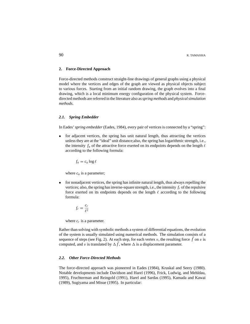
Force-directed methods construct straight-line drawings of general graphs using a physicalmodel where the vertices and edges of the graph are viewed as physical objects subjectto various forces. Starting from an initial random drawing, the graph evolves into a finaldrawing, which is a local minimum energy configuration of the physical system. Force-directed methods are referred in the literature also asspring methodsandphysical simulationmethods.

2.1. Spring Embedder

In Eades’spring embedder(Eades, 1984), every pair of vertices is connected by a “spring”:

• for adjacent vertices, the spring has unit natural length, thus attracting the verticesunless they are at the “ideal” unit distance;also, the spring has logarithmic strength, i.e.,the intensityfa of the attractive force exerted on its endpoints depends on the length`

according to the following formula:

fa = ca log`

whereca is a parameter;

• for nonadjacent vertices, the spring has infinite natural length, thus always repelling thevertices; also, the spring has inverse-square strength, i.e., the intensityfr of the repulsiveforce exerted on its endpoints depends on the length` according to the followingformula:

fr = cr

`2

wherecr is a parameter.

Rather than solving with symbolic methods a system of differential equations, the evolutionof the system is usually simulated using numerical methods. The simulation consists of asequence of steps (see Fig. 2). At each step, for each vertexv, the resulting forceEf onv iscomputed, andv is translated by1 Ef , where1 is a displacement parameter.

2.2. Other Force-Directed Methods

The force-directed approach was pioneered in Eades (1984), Kruskal and Seery (1980).Notable developments include Davidson and Harel (1996), Frick, Ludwig, and Mehldau,1995), Fruchterman and Reingold (1991), Harel and Sardas (1995), Kamada and Kawai(1989), Sugiyama and Misue (1995). In particular:


(b)

(a)

(c)

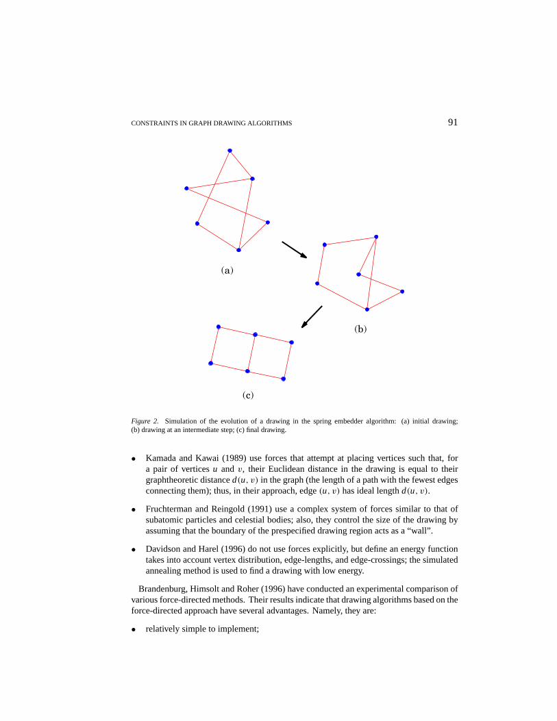
Figure 2. Simulation of the evolution of a drawing in the spring embedder algorithm: (a) initial drawing;(b) drawing at an intermediate step; (c) final drawing.

• Kamada and Kawai (1989) use forces that attempt at placing vertices such that, fora pair of verticesu andv, their Euclidean distance in the drawing is equal to theirgraphtheoretic distanced(u, v) in the graph (the length of a path with the fewest edgesconnecting them); thus, in their approach, edge(u, v) has ideal lengthd(u, v).

• Fruchterman and Reingold (1991) use a complex system of forces similar to that ofsubatomic particles and celestial bodies; also, they control the size of the drawing byassuming that the boundary of the prespecified drawing region acts as a “wall”.

• Davidson and Harel (1996) do not use forces explicitly, but define an energy functiontakes into account vertex distribution, edge-lengths, and edge-crossings; the simulatedannealing method is used to find a drawing with low energy.

Brandenburg, Himsolt and Roher (1996) have conducted an experimental comparison ofvarious force-directed methods. Their results indicate that drawing algorithms based on theforce-directed approach have several advantages. Namely, they are:

• relatively simple to implement;

92 R. TAMASSIA

• straightforward to parameterize;

• easy to extend by adding new forces;

• usually effective for small graphs with regular structure;

• often able to detect and display symmetries in the graph (see, e.g., Fig. 2);

• capable of preserving the user’s “mental map” by providing a continuous evolution ofthe drawing from the initial to the final configuration.

Disadvantages include:

• the running time for large graphs is rather slow;

• only straight-line drawings are supported;

• the properties of the generated drawings (e.g., area, crossings) are difficult to analyzetheoretically.

2.3. Constraints in the Force-Directed Approach

The force-directed approach has been extended to support several types of constraints inDengler, Friedell, and Marks (1993), He and Marriott (1997), Kamps, Kleinz, and Read(1996), Ryall, Marks, and Shieber (1997), Sugiyama and Misue (1995). Simple extensionsare mentioned below. For more sophisticated extensions, see Section 7.

Three types of constraints can be easily supported within the force-directed approach:

• position constraints;

• fixed-subgraph constraints; and

• constraints that can be expressed by forces or energy functions.

A position constraint assigns to a vertex a topologically connected region where the vertexshould remain. Examples of prescribed regions include:

1. a single point, equivalent to “pinning down” the vertex at a specific location;

2. a line, equivalent to assigning a “layer” to the vertex;

3. a circle, which allows to place groups of vertices into distinct regions.

Position constraints are immediate to satisfy by confining to the prescribed region thetranslation of the vertex at each simulation step.

A fixed-subgraph constraint assigns to a subgraph a prescribed subdrawing, which mayappear translated or rotated, but not otherwise deformed, in the overall drawing of the graph.It can be supported by considering the subgraph as a rigid body, which gets translated androtated at each simulation step according to the overall force and torque applied to it as aresult of the individual forces applied to its vertices.

Constraints that can be expressed by forces include:


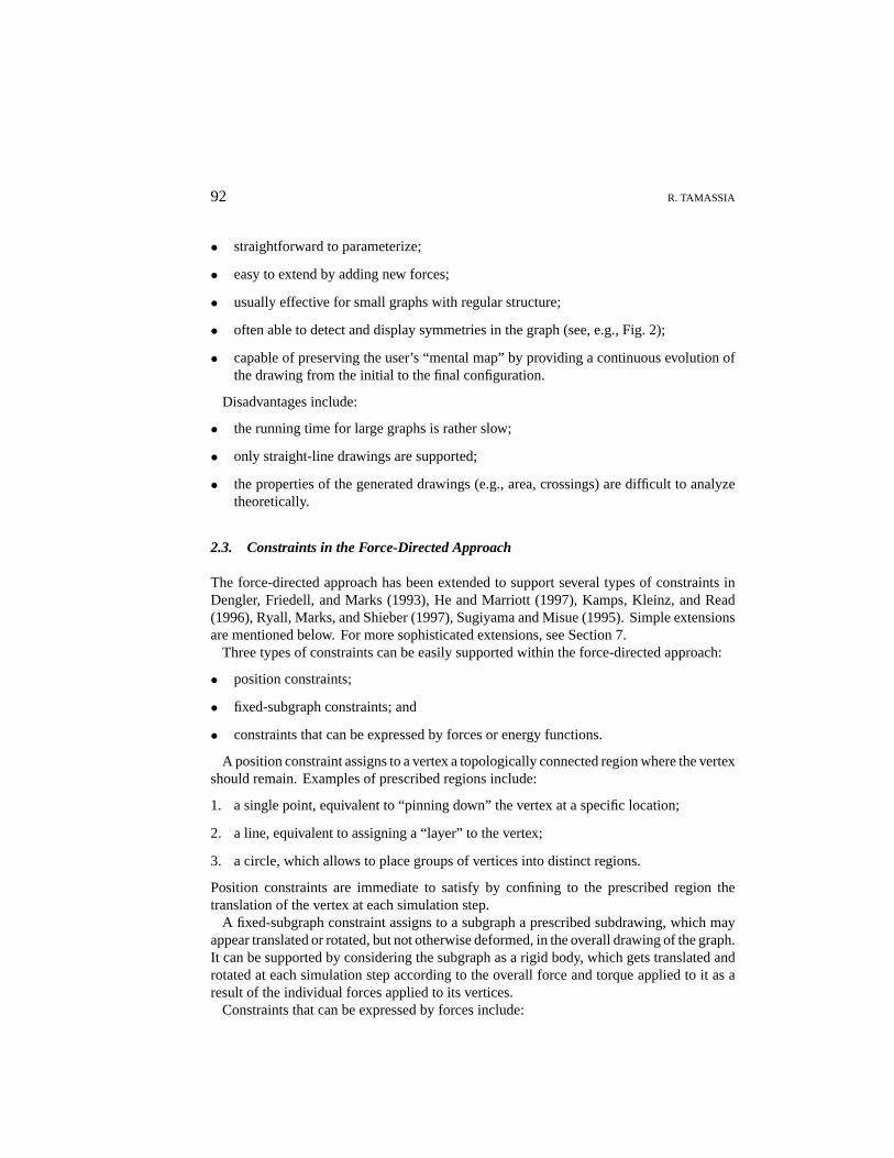
Figure 3. Example of clustering constraints realized by means of forces: the two shaded vertices represent thedummy attractors of the two clusters; the attractive forces between cluster vertices and attractors, and the repulsiveforce between attractors are shown with dashed double-arrows.

• clustering of vertices;

• alignment of vertices;

• orientation of directed edges.

Clustering can be achieved as follows (see Fig. 3):

1. for each cluster, add to the graph a dummy “attractor” vertex;

2. add attractive forces between an attractor and each vertex in the attractor’s cluster;

3. add repulsive forces between pairs of attractors and between attractors and vertices notin any cluster.

Forces that simulate a parallel “magnetic field” can be used to orient the edges accordingto a general direction, e.g., upward. Namely, a torque is applied to the edges that tendsto align them with the field lines. This approach was recently presented in Sugiyama andMisue (1995).

2.4. Barycentric Method

We now show that a classical drawing algorithm for planar graphs, thebarycentric methodby Tutte (1960, 1963), can be reinterpreted as a constrained force-directed method.

Let G be a triconnected graph, and letγ be a nonseparating cycle ofG, i.e., a cyclewhose removal does not disconnectG. The barycentric method draws firstγ as a convexpolygon0. Then, for each vertexv not inγ , it writes the followingbarycentric equations,which express the fact that vertexv is in the barycenter (centroid) of its neighbors:

x(v) = 1

deg(v)

∑w adj. to v

x(w) (1)

y(v) = 1

deg(v)

∑w adj. to v

y(w) (2)

94 R. TAMASSIA

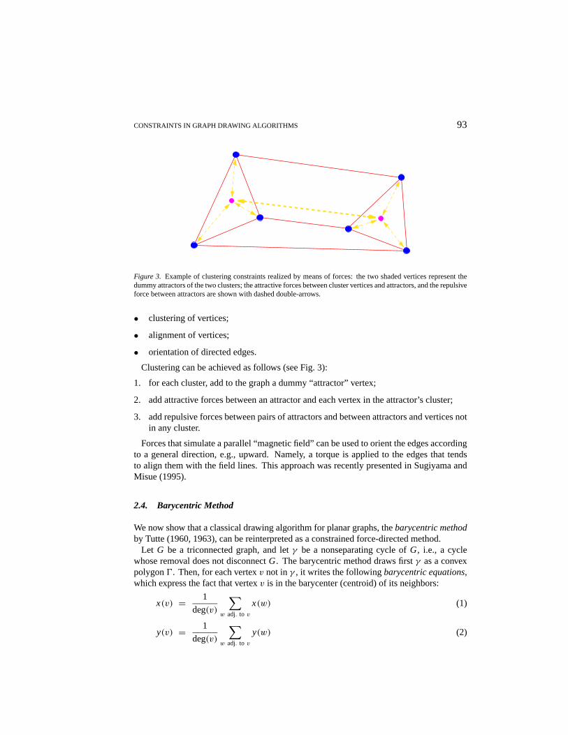
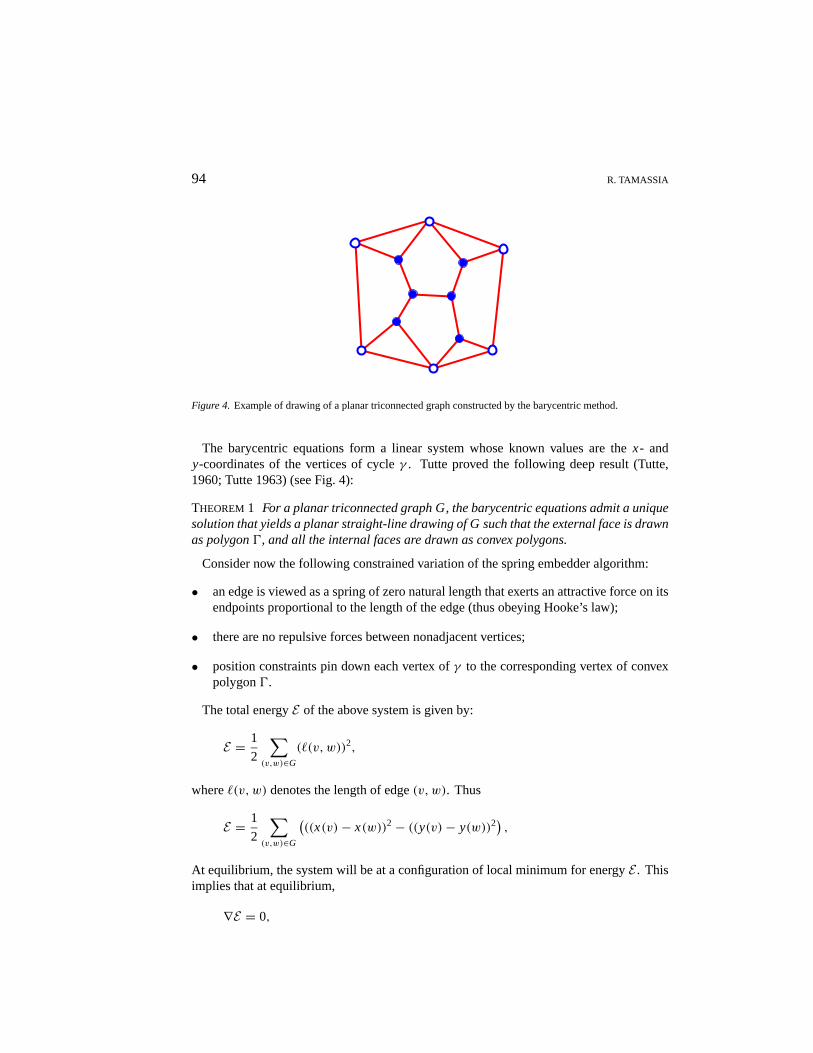
Figure 4. Example of drawing of a planar triconnected graph constructed by the barycentric method.

The barycentric equations form a linear system whose known values are thex- andy-coordinates of the vertices of cycleγ . Tutte proved the following deep result (Tutte,1960; Tutte 1963) (see Fig. 4):

THEOREM1 For a planar triconnected graph G, the barycentric equations admit a uniquesolution that yields a planar straight-line drawing of G such that the external face is drawnas polygon0, and all the internal faces are drawn as convex polygons.

Consider now the following constrained variation of the spring embedder algorithm:

• an edge is viewed as a spring of zero natural length that exerts an attractive force on itsendpoints proportional to the length of the edge (thus obeying Hooke’s law);

• there are no repulsive forces between nonadjacent vertices;

• position constraints pin down each vertex ofγ to the corresponding vertex of convexpolygon0.

The total energyE of the above system is given by:

E = 1

2

∑(v,w)∈G

(`(v,w))2,

where`(v,w) denotes the length of edge(v,w). Thus

E = 1

2

∑(v,w)∈G

(((x(v)− x(w))2− ((y(v)− y(w))2

),

At equilibrium, the system will be at a configuration of local minimum for energyE . Thisimplies that at equilibrium,

∇E = 0,


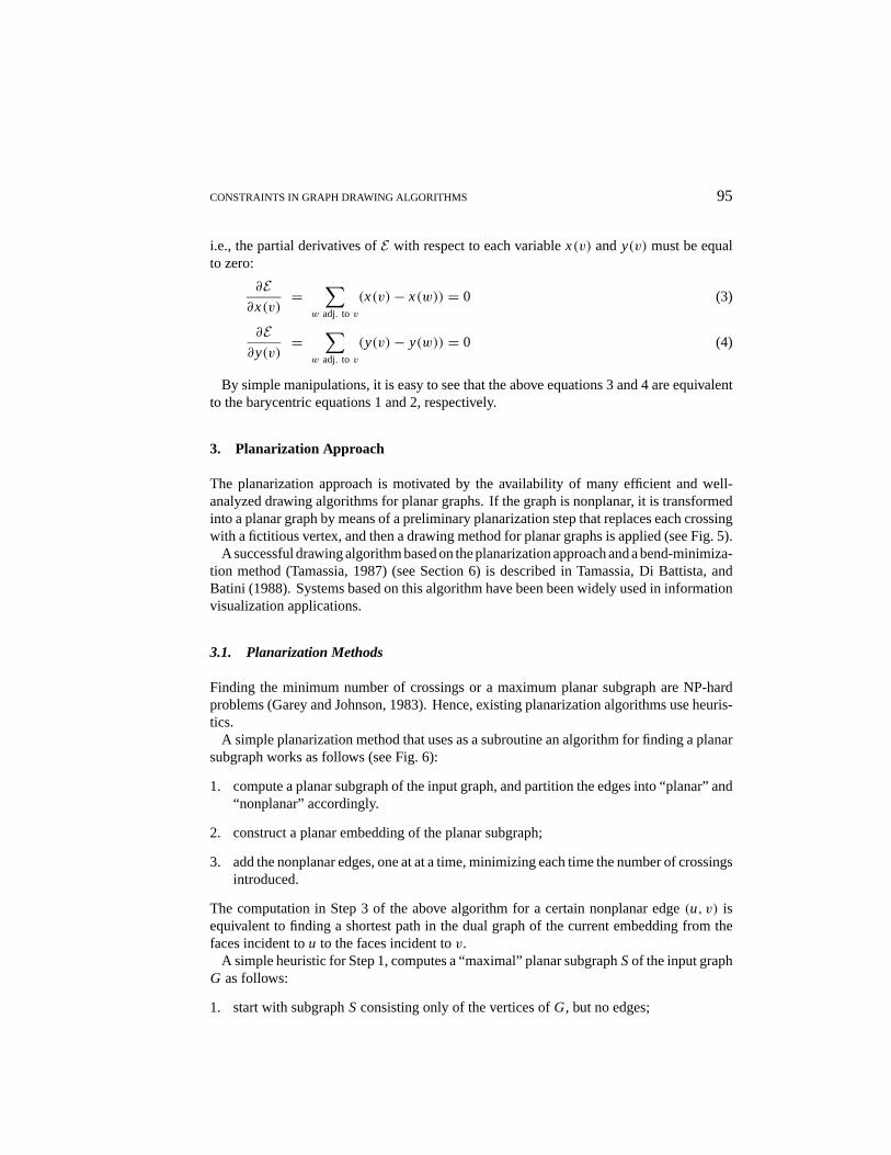
i.e., the partial derivatives ofE with respect to each variablex(v) andy(v) must be equalto zero:

∂E∂x(v)

=∑

w adj. to v

(x(v)− x(w)) = 0 (3)

∂E∂y(v)

=∑

w adj. to v

(y(v)− y(w)) = 0 (4)

By simple manipulations, it is easy to see that the above equations 3 and 4 are equivalentto the barycentric equations 1 and 2, respectively.

3. Planarization Approach

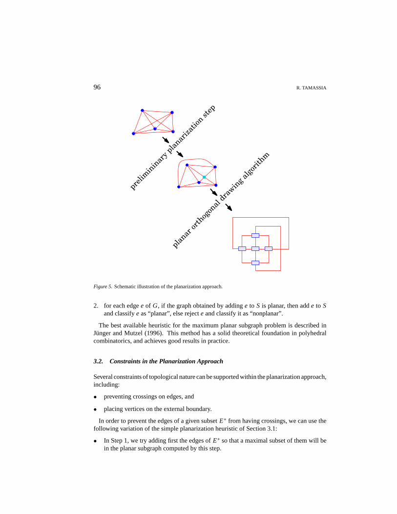
The planarization approach is motivated by the availability of many efficient and well-analyzed drawing algorithms for planar graphs. If the graph is nonplanar, it is transformedinto a planar graph by means of a preliminary planarization step that replaces each crossingwith a fictitious vertex, and then a drawing method for planar graphs is applied (see Fig. 5).

A successful drawing algorithm based on the planarization approach and a bend-minimiza-tion method (Tamassia, 1987) (see Section 6) is described in Tamassia, Di Battista, andBatini (1988). Systems based on this algorithm have been been widely used in informationvisualization applications.

3.1. Planarization Methods

Finding the minimum number of crossings or a maximum planar subgraph are NP-hardproblems (Garey and Johnson, 1983). Hence, existing planarization algorithms use heuris-tics.

A simple planarization method that uses as a subroutine an algorithm for finding a planarsubgraph works as follows (see Fig. 6):

1. compute a planar subgraph of the input graph, and partition the edges into “planar” and“nonplanar” accordingly.

2. construct a planar embedding of the planar subgraph;

3. add the nonplanar edges, one at at a time, minimizing each time the number of crossingsintroduced.

The computation in Step 3 of the above algorithm for a certain nonplanar edge(u, v) isequivalent to finding a shortest path in the dual graph of the current embedding from thefaces incident tou to the faces incident tov.

A simple heuristic for Step 1, computes a “maximal” planar subgraphSof the input graphG as follows:

1. start with subgraphSconsisting only of the vertices ofG, but no edges;

96 R. TAMASSIA

preli

min

inar

y pla

nariza

tion st

ep

plan

ar or

thog

onal

drawin

g algo

rithm

Figure 5. Schematic illustration of the planarization approach.

2. for each edgee of G, if the graph obtained by addinge to S is planar, then adde to Sand classifye as “planar”, else rejecte and classify it as “nonplanar”.

The best available heuristic for the maximum planar subgraph problem is described inJunger and Mutzel (1996). This method has a solid theoretical foundation in polyhedralcombinatorics, and achieves good results in practice.

3.2. Constraints in the Planarization Approach

Several constraints of topological nature can be supported within the planarization approach,including:

• preventing crossings on edges, and

• placing vertices on the external boundary.

In order to prevent the edges of a given subsetE∗ from having crossings, we can use thefollowing variation of the simple planarization heuristic of Section 3.1:

• In Step 1, we try adding first the edges ofE∗ so that a maximal subset of them will bein the planar subgraph computed by this step.


(a)

(c)

(b)

(d)

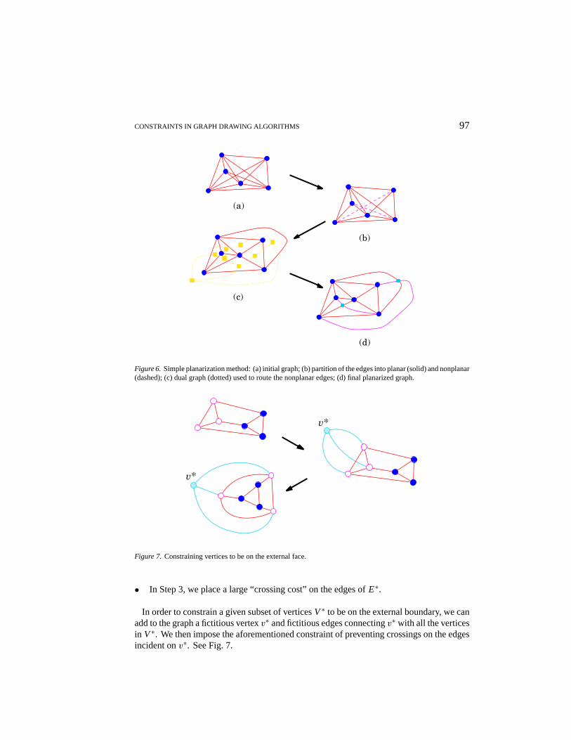
Figure 6. Simple planarization method: (a) initial graph; (b) partition of the edges into planar (solid) and nonplanar(dashed); (c) dual graph (dotted) used to route the nonplanar edges; (d) final planarized graph.

v*

v*

Figure 7. Constraining vertices to be on the external face.

• In Step 3, we place a large “crossing cost” on the edges ofE∗.

In order to constrain a given subset of verticesV∗ to be on the external boundary, we canadd to the graph a fictitious vertexv∗ and fictitious edges connectingv∗ with all the verticesin V∗. We then impose the aforementioned constraint of preventing crossings on the edgesincident onv∗. See Fig. 7.

98 R. TAMASSIA

4. Visibility Representations and Planar Polyline Drawings

We start by recalling some definitions on numberings and orientations of digraphs, whichare used in the drawing techniques discussed in this section.

4.1. Properties of Planar Directed Graphs

Let G be a directed graph withn vertices. Atopological numberingof G is an assignmentof numbers to the vertices ofG such that, for every edge(u, v) of G, the number assignedto v is greater than the one assigned tou (i.e., number(v) > number(u)). A topologicalsortingis a topological numbering ofG such that every vertex is assigned a distinct integerbetween 1 andn. A topological sorting is not unique unlessG has a directed path that visitsevery vertex. It is easy to show that the following statements are equivalent:

• G is acyclic;

• G admits a topological numbering;

• G admits a topological sorting.

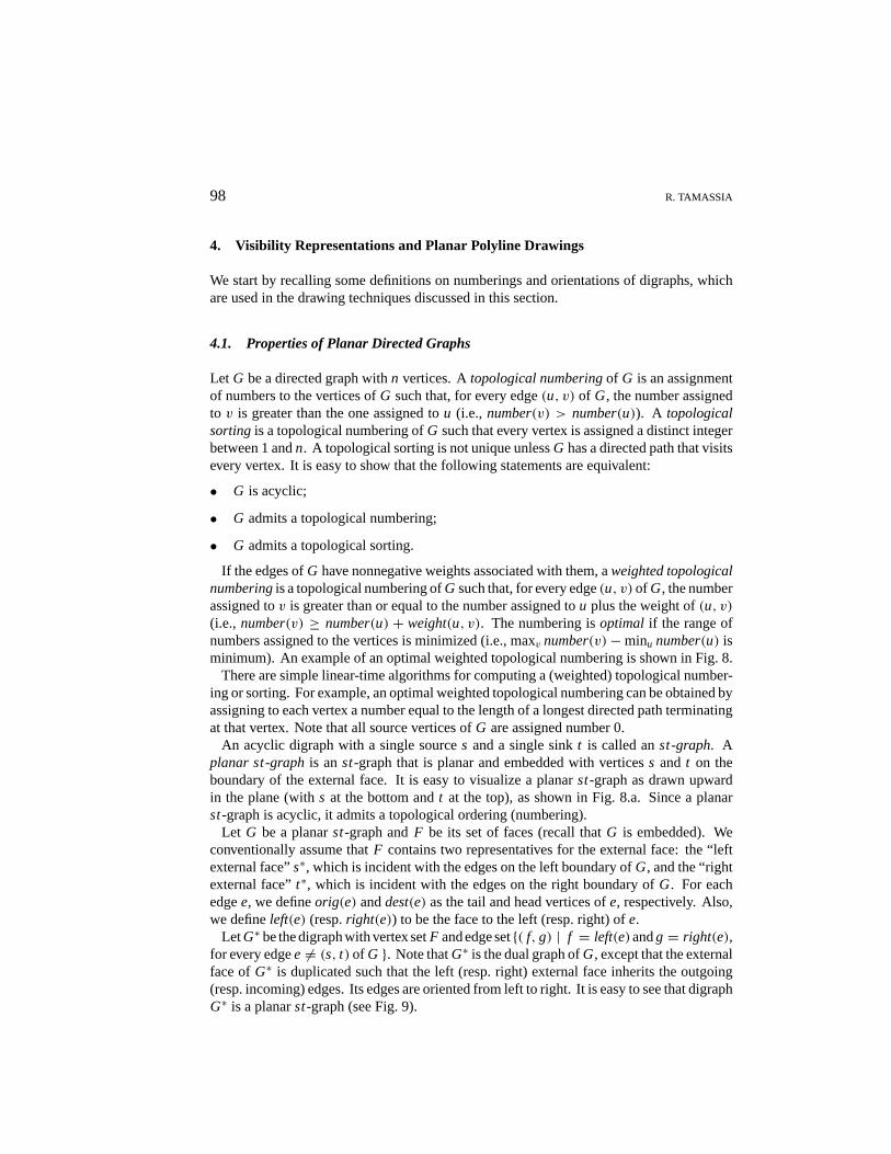
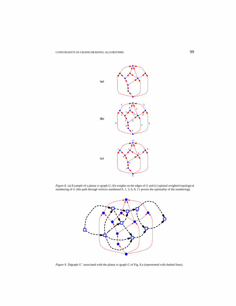
If the edges ofG have nonnegative weights associated with them, aweighted topologicalnumberingis a topological numbering ofG such that, for every edge(u, v) of G, the numberassigned tov is greater than or equal to the number assigned tou plus the weight of(u, v)(i.e., number(v) ≥ number(u) + weight(u, v). The numbering isoptimal if the range ofnumbers assigned to the vertices is minimized (i.e., maxv number(v)−minu number(u) isminimum). An example of an optimal weighted topological numbering is shown in Fig. 8.

There are simple linear-time algorithms for computing a (weighted) topological number-ing or sorting. For example, an optimal weighted topological numbering can be obtained byassigning to each vertex a number equal to the length of a longest directed path terminatingat that vertex. Note that all source vertices ofG are assigned number 0.

An acyclic digraph with a single sources and a single sinkt is called anst-graph. Aplanar st-graphis anst-graph that is planar and embedded with verticess and t on theboundary of the external face. It is easy to visualize a planarst-graph as drawn upwardin the plane (withs at the bottom andt at the top), as shown in Fig. 8.a. Since a planarst-graph is acyclic, it admits a topological ordering (numbering).

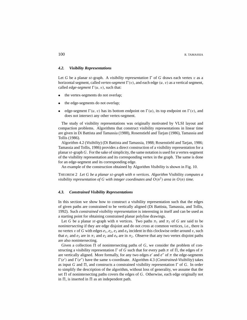
Let G be a planarst-graph andF be its set of faces (recall thatG is embedded). Weconventionally assume thatF contains two representatives for the external face: the “leftexternal face”s∗, which is incident with the edges on the left boundary ofG, and the “rightexternal face”t∗, which is incident with the edges on the right boundary ofG. For eachedgee, we defineorig(e) anddest(e) as the tail and head vertices ofe, respectively. Also,we defineleft(e) (resp.right(e)) to be the face to the left (resp. right) ofe.

LetG∗ be the digraph with vertex setF and edge set{( f, g) | f = left(e)andg = right(e),for every edgee 6= (s, t) of G }. Note thatG∗ is the dual graph ofG, except that the externalface ofG∗ is duplicated such that the left (resp. right) external face inherits the outgoing(resp. incoming) edges. Its edges are oriented from left to right. It is easy to see that digraphG∗ is a planarst-graph (see Fig. 9).


(a)

(b)6

3

4

1

3 1

3

2

45

2

1

31

1

(c)

11

0

1

3

6

87 7

4

Figure 8. (a) Example of a planarst-graphG; (b) weights on the edges ofG and (c) optimal weighted topologicalnumbering ofG (the path through vertices numbered 0, 1, 3, 6, 8, 11 proves the optimality of the numbering).

Figure 9. DigraphG∗ associated with the planarst-graphG of Fig. 8.a (represented with dashed lines).

100 R. TAMASSIA

4.2. Visibility Representations

Let G be a planarst-graph. Avisibility representation0 of G draws each vertexv as ahorizontal segment, calledvertex-segment0(v), and each edge(u, v) as a vertical segment,callededge-segment0(u, v), such that:

• the vertex-segments do not overlap;

• the edge-segments do not overlap;

• edge-segment0(u, v) has its bottom endpoint on0(u), its top endpoint on0(v), anddoes not intersect any other vertex-segment.

The study of visibility representations was originally motivated by VLSI layout andcompaction problems. Algorithms that construct visibility representations in linear timeare given in Di Battista and Tamassia (1988), Rosenstiehl and Tarjan (1986), Tamassia andTollis (1986).

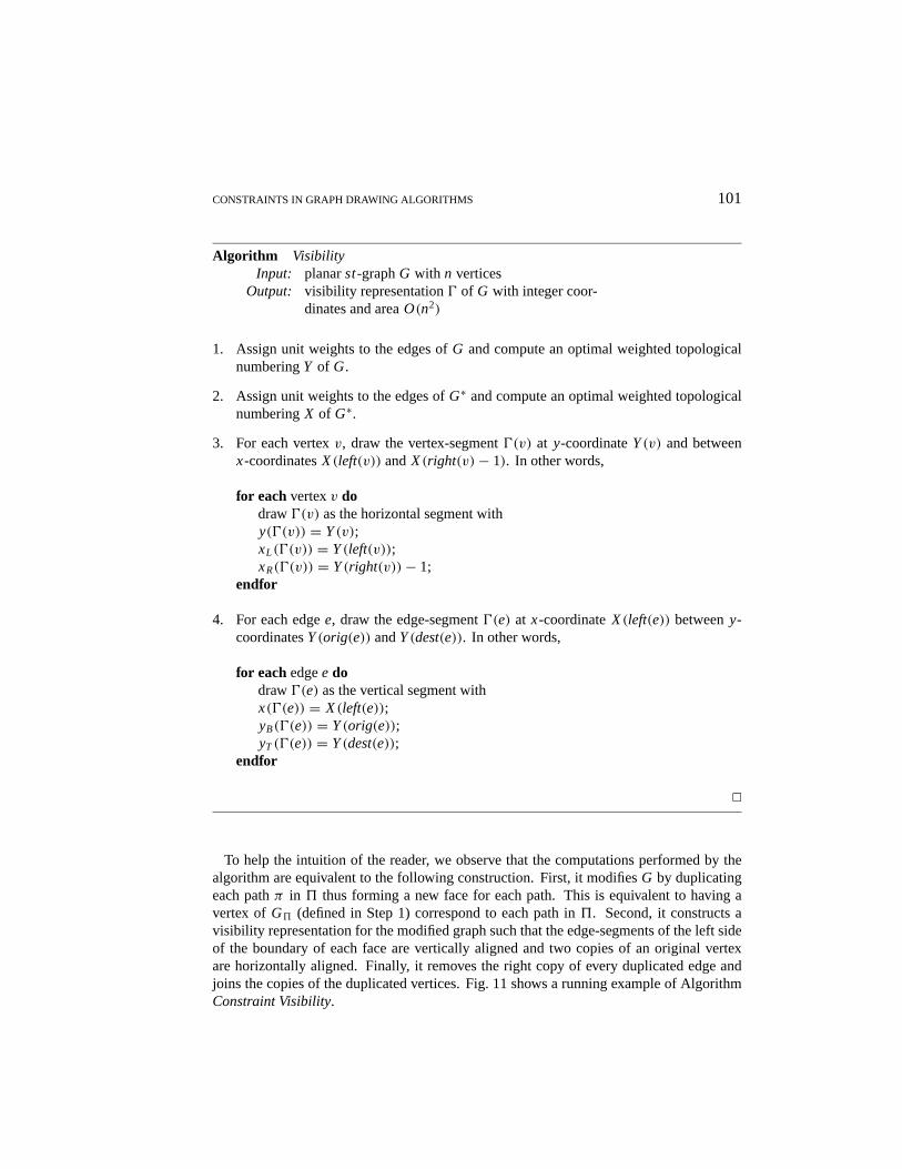
Algorithm 4.2 (Visibility) (Di Battista and Tamassia, 1988; Rosenstiehl and Tarjan, 1986;Tamassia and Tollis, 1986) provides a direct construction of a visibility representation for aplanarst-graphG. For the sake of simplicity, the same notation is used for a vertex-segmentof the visibility representation and its corresponding vertex in the graph. The same is donefor an edge-segment and its corresponding edge.

An example of the construction obtained by AlgorithmVisibility is shown in Fig. 10.

THEOREM2 Let G be a planar st-graph with n vertices. AlgorithmVisibility computes avisibility representation of G with integer coordinates and O(n2) area in O(n) time.

4.3. Constrained Visibility Representations

In this section we show how to construct a visibility representation such that the edgesof given paths are constrained to be vertically aligned (Di Battista, Tamassia, and Tollis,1992). Suchconstrained visibility representationis interesting in itself and can be used asa starting point for obtaining constrained planar polyline drawings.

Let G be a planarst-graph withn vertices. Two pathsπ1 andπ2 of G are said to benonintersectingif they are edge disjoint and do notcrossat common vertices, i.e., there isno vertexv of G with edgese1, e2, e3 ande4 incident in this clockwise order aroundv, suchthate1 ande3 are inπ1 ande2 ande4 are inπ2. Observe that any two vertex disjoint pathsare also nonintersecting.

Given a collection5 of nonintersecting paths ofG, we consider the problem of con-structing a visibility representation0 of G such that for every pathπ of 5, the edges ofπare vertically aligned. More formally, for any two edgese′ ande′′ of π the edge-segments0(e′) and0(e′′) have the same x-coordinate. Algorithm 4.3 (Constrained-Visibility) takesas inputG and5, and constructs a constrained visibility representation0 of G. In orderto simplify the description of the algorithm, without loss of generality, we assume that theset5 of nonintersecting paths covers the edges ofG. Otherwise, each edge originally notin 5, is inserted in5 as an independent path.


Algorithm VisibilityInput: planarst-graphG with n vertices

Output: visibility representation0 of G with integer coor-dinates and areaO(n2)

1. Assign unit weights to the edges ofG and compute an optimal weighted topologicalnumberingY of G.

2. Assign unit weights to the edges ofG∗ and compute an optimal weighted topologicalnumberingX of G∗.

3. For each vertexv, draw the vertex-segment0(v) at y-coordinateY(v) and betweenx-coordinatesX(left(v)) andX(right(v)− 1). In other words,

for eachvertexv dodraw0(v) as the horizontal segment withy(0(v)) = Y(v);xL(0(v)) = Y(left(v));xR(0(v)) = Y(right(v))− 1;

endfor

4. For each edgee, draw the edge-segment0(e) at x-coordinateX(left(e)) betweeny-coordinatesY(orig(e)) andY(dest(e)). In other words,

for eachedgee dodraw0(e) as the vertical segment withx(0(e)) = X(left(e));yB(0(e)) = Y(orig(e));yT (0(e)) = Y(dest(e));

endfor

2

To help the intuition of the reader, we observe that the computations performed by thealgorithm are equivalent to the following construction. First, it modifiesG by duplicatingeach pathπ in 5 thus forming a new face for each path. This is equivalent to having avertex ofG5 (defined in Step 1) correspond to each path in5. Second, it constructs avisibility representation for the modified graph such that the edge-segments of the left sideof the boundary of each face are vertically aligned and two copies of an original vertexare horizontally aligned. Finally, it removes the right copy of every duplicated edge andjoins the copies of the duplicated vertices. Fig. 11 shows a running example of AlgorithmConstraint Visibility.

102 R. TAMASSIA

(b)

(a)

0 1 3 4 5 6 720

1

3

4

5

2

0

1

0

5

7

4

6

2 4

3

52

1

3 3

44 4

Figure 10. Example of a visibility representation constructed by AlgorithmVisibility: (a) a planarst-graphG(drawn with solid lines), its dualG∗ (drawn with dashed lines), and the numberings ofG andG∗ (shown as labels);(b) a visibility representation forG, where the vertices are represeneted by horizontal segments and the edges arerepresented by vertical segments.

THEOREM3 Let G be a planar st-graph with n vertices, and5 be a set of nonintersectingpaths covering the edges of G. AlgorithmConstrained Visibilitycomputes in O(n) time avisibility representation of G with integer coordinates and O(n2) area, such that the edgesof every pathπ in 5 are vertically aligned.

5. Polyline Drawings from Visibility Representations

We can construct a planar upward polyline drawing of a planarst-graphG starting from avisibility representation ofG as follows (Di Battista and Tamassia, 1988): we draw eachvertex ofG at an arbitrary point of its vertex-segment, and each edge(u, v) of G as a three-segment polygonal chain whose middle segment is a subset of the edge-segment of(u, v).E.g., a possible choice for the placement ofP(v) is the middle point of vertex-segment


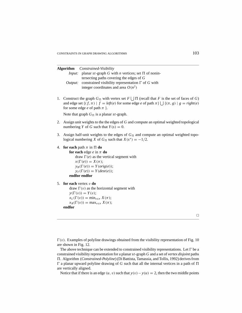
Algorithm Constrained-VisibilityInput: planarst-graphG with n vertices; set5 of nonin-

tersecting paths covering the edges ofGOutput: constrained visibility representation0 of G with

integer coordinates and areaO(n2)

1. Construct the graphG5 with vertex setF⋃5 (recall thatF is the set of faces ofG)

and edge set{( f, π) | f = left(e) for some edgee of pathπ}⋃ {(π, g) | g = right(e)for some edgee of pathπ }.Note that graphG5 is a planarst-graph.

2. Assign unit weights to the the edges ofG and compute an optimal weighted topologicalnumberingY of G such thatY(s) = 0.

3. Assign half-unit weights to the edges ofG5 and compute an optimal weighted topo-logical numberingX of G5 such thatX(s∗) = −1/2.

4. for eachpathπ in 5 dofor eachedgee in π do

draw0(e) as the vertical segment withx(0(e)) = X(π);yB(0(e)) = Y(orig(e));yT (0(e)) = Y(dest(e));

endfor endfor

5. for eachvertexv dodraw0(v) as the horizontal segment withy(0(v)) = Y(v);xL(0(v)) = minv∈π X(π);xR(0(v)) = maxv∈π X(π);

endfor

2

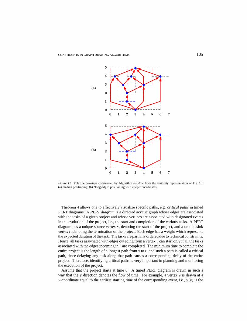
0(v). Examples of polyline drawings obtained from the visibility representation of Fig. 10are shown in Fig. 12.

The above technique can be extended to constrained visibility representations. Let0 be aconstrained visibility representation for a planarst-graphG and a set ofvertex disjointpaths5. Algorithm (Constrained-Polyline) (Di Battista, Tamassia, and Tollis, 1992) derives from0 a planar upward polyline drawing ofG such that all the internal vertices in a path of5

are vertically aligned.Notice that if there is an edge(u, v) such thaty(v)− y(u) = 2, then the two middle points

104 R. TAMASSIA

(c)

(a)

0 1 3 4 5 6 720

1

3

4

5

2

-0.50.5

0

5

7.5

4

6.5

2

5.5

0

4.51.5

1

3 3

4

4 4

(b)

2.5

67

4

1 2 3

3.5

5

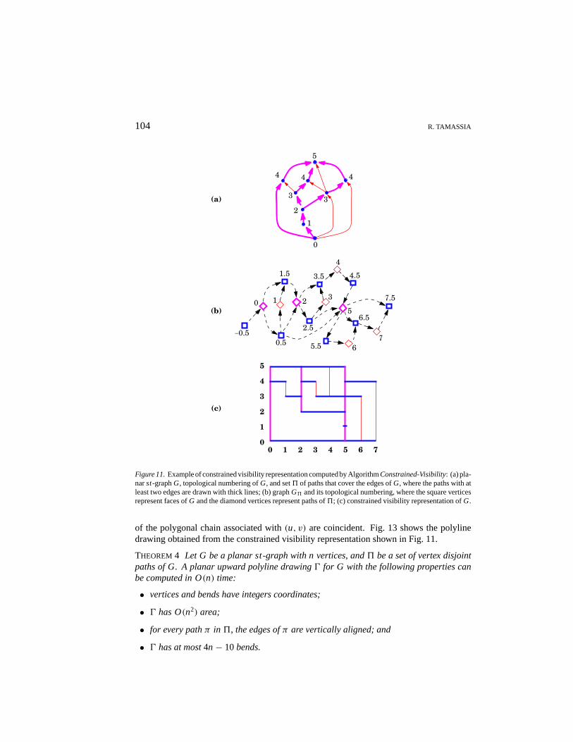
Figure 11.Example of constrained visibility representation computed by AlgorithmConstrained-Visibility: (a) pla-narst-graphG, topological numbering ofG, and set5 of paths that cover the edges ofG, where the paths with atleast two edges are drawn with thick lines; (b) graphG5 and its topological numbering, where the square verticesrepresent faces ofG and the diamond vertices represent paths of5; (c) constrained visibility representation ofG.

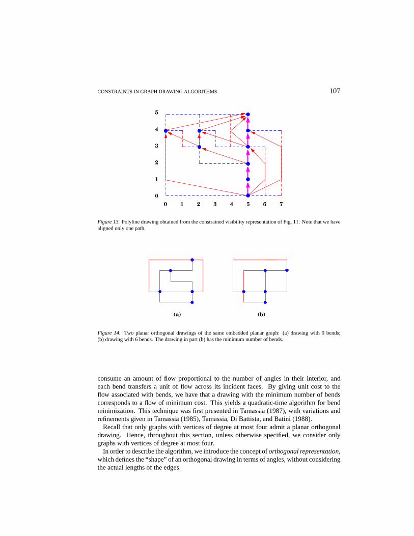
of the polygonal chain associated with(u, v) are coincident. Fig. 13 shows the polylinedrawing obtained from the constrained visibility representation shown in Fig. 11.

THEOREM4 Let G be a planar st-graph with n vertices, and5 be a set of vertex disjointpaths of G. A planar upward polyline drawing0 for G with the following properties canbe computed in O(n) time:

• vertices and bends have integers coordinates;

• 0 has O(n2) area;

• for every pathπ in 5, the edges ofπ are vertically aligned; and

• 0 has at most4n− 10bends.


(a)

0 1 3 4 5 6 720

1

3

4

5

2

(b)

0 1 3 4 5 6 720

1

3

4

5

2

Figure 12. Polyline drawings constructed by AlgorithmPolyline from the visibility representation of Fig. 10:(a) median positioning; (b) “long-edge” positioning with integer coordinates.

Theorem 4 allows one to effectively visualize specific paths, e.g.critical pathsin timedPERT diagrams. APERT diagramis a directed acyclic graph whose edges are associatedwith the tasks of a given project and whose vertices are associated with designated eventsin the evolution of the project, i.e., the start and completion of the various tasks. A PERTdiagram has a unique source vertexs, denoting the start of the project, and a unique sinkvertext , denoting the termination of the project. Each edge has a weight which representsthe expected duration of the task. The tasks are partially ordered due to technical constraints.Hence, all tasks associated with edges outgoing from a vertexv can start only if all the tasksassociated with the edges incoming inv are completed. The minimum time to complete theentire project is the length of a longest path froms to t , and such a path is called a criticalpath, since delaying any task along that path causes a corresponding delay of the entireproject. Therefore, identifying critical paths is very important in planning and monitoringthe execution of the project.

Assume that the project starts at time 0. A timed PERT diagram is drawn in such away that they direction denotes the flow of time. For example, a vertexv is drawn at ay-coordinate equal to the earliest starting time of the corresponding event, i.e.,y(v) is the

106 R. TAMASSIA

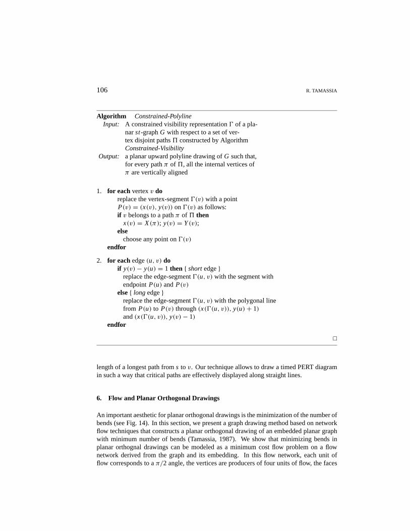
Algorithm Constrained-PolylineInput: A constrained visibility representation0 of a pla-

narst-graphG with respect to a set of ver-tex disjoint paths5 constructed by AlgorithmConstrained-Visibility

Output: a planar upward polyline drawing ofG such that,for every pathπ of 5, all the internal vertices ofπ are vertically aligned

1. for eachvertexv doreplace the vertex-segment0(v) with a pointP(v) = (x(v), y(v)) on0(v) as follows:if v belongs to a pathπ of 5 then

x(v) = X(π); y(v) = Y(v);else

choose any point on0(v)endfor

2. for eachedge(u, v) doif y(v)− y(u) = 1 then { shortedge}

replace the edge-segment0(u, v) with the segment withendpointP(u) andP(v)

else{ longedge}replace the edge-segment0(u, v) with the polygonal linefrom P(u) to P(v) through(x(0(u, v)), y(u)+ 1)and(x(0(u, v)), y(v)− 1)

endfor

2

length of a longest path froms to v. Our technique allows to draw a timed PERT diagramin such a way that critical paths are effectively displayed along straight lines.

6. Flow and Planar Orthogonal Drawings

An important aesthetic for planar orthogonal drawings is the minimization of the number ofbends (see Fig. 14). In this section, we present a graph drawing method based on networkflow techniques that constructs a planar orthogonal drawing of an embedded planar graphwith minimum number of bends (Tamassia, 1987). We show that minimizing bends inplanar orthognal drawings can be modeled as a minimum cost flow problem on a flownetwork derived from the graph and its embedding. In this flow network, each unit offlow corresponds to aπ/2 angle, the vertices are producers of four units of flow, the faces


0 1 3 4 5 6 720

1

3

4

5

2

Figure 13.Polyline drawing obtained from the constrained visibility representation of Fig. 11. Note that we havealigned only one path.

(a) (b)

Figure 14. Two planar orthogonal drawings of the same embedded planar graph: (a) drawing with 9 bends;(b) drawing with 6 bends. The drawing in part (b) has the minimum number of bends.

consume an amount of flow proportional to the number of angles in their interior, andeach bend transfers a unit of flow across its incident faces. By giving unit cost to theflow associated with bends, we have that a drawing with the minimum number of bendscorresponds to a flow of minimum cost. This yields a quadratic-time algorithm for bendminimization. This technique was first presented in Tamassia (1987), with variations andrefinements given in Tamassia (1985), Tamassia, Di Battista, and Batini (1988).

Recall that only graphs with vertices of degree at most four admit a planar orthogonaldrawing. Hence, throughout this section, unless otherwise specified, we consider onlygraphs with vertices of degree at most four.

In order to describe the algorithm, we introduce the concept oforthogonal representation,which defines the “shape” of an orthogonal drawing in terms of angles, without consideringthe actual lengths of the edges.

108 R. TAMASSIA

6.1. Orthogonal Representation

In this section, we introduce the concept of orthogonal representation, which captures thenotion of “orthogonal shape” of a planar orthogonal drawing by taking into account anglesbut disregarding edge lengths.

Let 0 be a planar orthogonal drawing of an embedded planar graphG. There are twotypes of angles in0:

• angles formed by two edges incident on a common vertex, calledvertex-angles; and

• angles formed by bends, calledbend-angles.

Let G be an embedded planar graph with vertices of degree at most four. We denotewith a( f ) the total number of vertex-angles inside facef of G. If G is biconnected,a( f )is equal to the number of vertices (edges) off . For each (undirected) edgee of G withendpointsu andv, we calldartsthe two possible orientations(u, v) and(v, u) of edgee. Adart is said to becounterclockwisewith respect to facef if f is on the left hand side whentraversing the dart from tail to head. We denote withD(v) the set of darts with vertexv astail, and withD( f ) the set of counterclockwise darts on facef .

An orthogonal representationof G is an assignment of integer valuesα(u, v) andβ(u, v)to each dart(u, v) of G such that:

• 1≤ α(u, v) ≤ 4;

• β(u, v) ≥ 0;

• for each vertexu, the sum ofα(u, v) over all the darts with tailv is equal to four, i.e.,∑(u,v)∈D(u)

α(u, v) = 4;

• for each internal facef , the sum ofα(u, v) + β(v, u) − β(u, v) over all the counter-clockwise darts(u, v) on face f is equal to 2a( f )− 4, i.e.,∑

(u,v)∈D( f )

α(u, v)+ β(v, u)− β(u, v) = 2a( f )− 4;

• for the external faceh, the above sum is equal to 2a(h)+ 4, i.e.,∑(u,v)∈D(h)

α(u, v)+ β(v, u)− β(u, v) = 2a(h)+ 4.

An orthogonal representation describes an equivalence class of orthogonal drawings with“similar shape”. More formally, an orthogonal drawing0 of G yields the following assign-ment of valuesα andβ to the darts ofG (see Fig 15.a):


(a)

(b) (c)

(1,0)(1,2)

(2,0)(1,2)

(2,1)(1,0)

(1,0)(1,1)

(1,1)(1,1)

(1,0)(1,0)

(2,1)(1,0)

(1,1)(2,0)

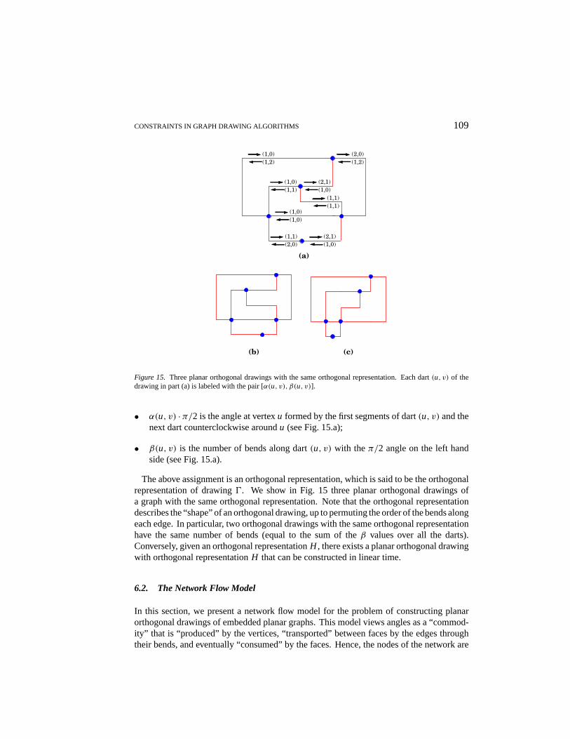
Figure 15. Three planar orthogonal drawings with the same orthogonal representation. Each dart(u, v) of thedrawing in part (a) is labeled with the pair [α(u, v), β(u, v)].

• α(u, v) ·π/2 is the angle at vertexu formed by the first segments of dart(u, v) and thenext dart counterclockwise aroundu (see Fig. 15.a);

• β(u, v) is the number of bends along dart(u, v) with theπ/2 angle on the left handside (see Fig. 15.a).

The above assignment is an orthogonal representation, which is said to be the orthogonalrepresentation of drawing0. We show in Fig. 15 three planar orthogonal drawings ofa graph with the same orthogonal representation. Note that the orthogonal representationdescribes the “shape” of an orthogonal drawing, up to permuting the order of the bends alongeach edge. In particular, two orthogonal drawings with the same orthogonal representationhave the same number of bends (equal to the sum of theβ values over all the darts).Conversely, given an orthogonal representationH , there exists a planar orthogonal drawingwith orthogonal representationH that can be constructed in linear time.

6.2. The Network Flow Model

In this section, we present a network flow model for the problem of constructing planarorthogonal drawings of embedded planar graphs. This model views angles as a “commod-ity” that is “produced” by the vertices, “transported” between faces by the edges throughtheir bends, and eventually “consumed” by the faces. Hence, the nodes of the network are

110 R. TAMASSIA

the vertices and faces of the graph. Since all angles we deal with have measurekπ/2, with1≤ k ≤ 4, we establish the convention that a unit of flow represents aπ/2 angle.

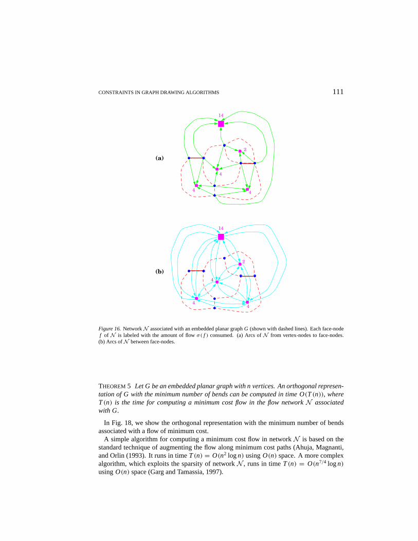
We associate with an embedded planar graphG a flow networkN whose nodes havesupplies and demands, and whose arcs have each a lower boundλ, a capacityµ, and acostχ , as follows (see Fig. 16):

• the nodes ofN are the vertices and faces ofG;

• a vertex-nodev of N produces flowσ(v) = 4;

• a face-nodef ofN consumes flowσ( f ) = 2a( f )−4 if f is an internal face, and flowσ(h) = 2a(h)+ 4 if f = h is the external face;

• for each dart(u, v) of G, with faces f andg on its left and right, respectively,N hastwo arcs(u, f ) and( f, g), where:

– arc(u, f ) has lower boundλ(u, f ) = 1, capacityµ(u, f ) = 4, and costχ(u, f ) =0 (see Fig. 16.a);

– arc ( f, g) has lower boundλ( f, g) = 0, capacityµ( f, g) = +∞, and costχ( f, g) = 1 (see Fig. 16.b).

The intuition behind the definition of flow networkN is as follows:

• the flow in arc(u, f ) associated with dart(u, v) represents the quantityα(u, v), i.e.,the measure of an angle formed at vertexu inside facef ;

• the flow in arc( f, g) associated with dart(u, v) represents the quantityβ(u, v), i.e.,the number bends with theπ/2 angle in facef along an edge between facesf andg;

• the conservation of flow at a vertex-node represents the geometric fact that the sum ofthe measures of the vertex-angles around a vertex is equal to 2π ;

• the conservation of flow at a face-node represents the geometric fact that the sum ofthe measures of the vertex-angles and bend-angles inside an internal facef is equal toπ(p− 2), wherep is the total number of such angles (iff is the external face, then theabove sum is equal toπ(p+ 2));

• the cost of the flow is equal to the number of bends.

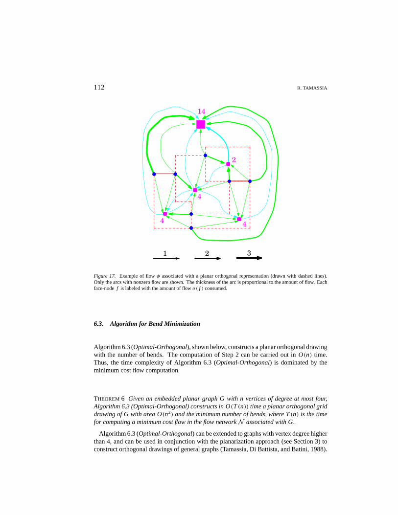
In the example of Fig. 17, we show the flow associated with a given orthogonal represen-tation.

An orthogonal representation ofG with the minimum number of bends can be computedas follows:

1. Construct the flow networkN associated withG.

2. Compute a flowφ of minimum cost for networkN .

3. Compute the orthogonal representation ofG associated withφ.


2

4

4

4

14

2

4

4

4

14

(a)

(b)

Figure 16.NetworkN associated with an embedded planar graphG (shown with dashed lines). Each face-nodef of N is labeled with the amount of flowσ( f ) consumed. (a) Arcs ofN from vertex-nodes to face-nodes.(b) Arcs ofN between face-nodes.

THEOREM5 Let G be an embedded planar graph with n vertices. An orthogonal represen-tation of G with the minimum number of bends can be computed in time O(T(n)), whereT(n) is the time for computing a minimum cost flow in the flow networkN associatedwith G.

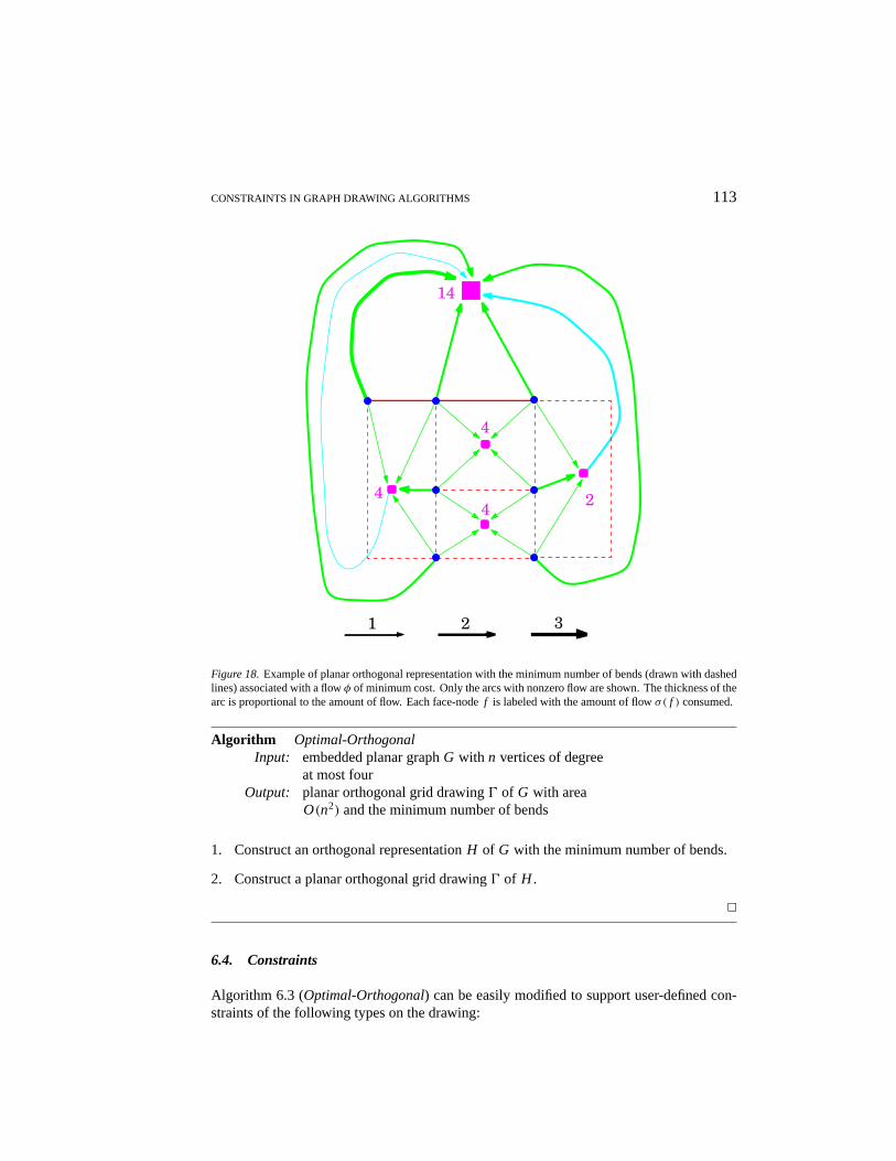
In Fig. 18, we show the orthogonal representation with the minimum number of bendsassociated with a flow of minimum cost.

A simple algorithm for computing a minimum cost flow in networkN is based on thestandard technique of augmenting the flow along minimum cost paths (Ahuja, Magnanti,and Orlin (1993). It runs in timeT(n) = O(n2 logn) usingO(n) space. A more complexalgorithm, which exploits the sparsity of networkN , runs in timeT(n) = O(n7/4 logn)usingO(n) space (Garg and Tamassia, 1997).

112 R. TAMASSIA

4

4 4

2

14

1 2 3

Figure 17. Example of flowφ associated with a planar orthogonal representation (drawn with dashed lines).Only the arcs with nonzero flow are shown. The thickness of the arc is proportional to the amount of flow. Eachface-nodef is labeled with the amount of flowσ( f ) consumed.

6.3. Algorithm for Bend Minimization

Algorithm 6.3 (Optimal-Orthogonal), shown below, constructs a planar orthogonal drawingwith the number of bends. The computation of Step 2 can be carried out inO(n) time.Thus, the time complexity of Algorithm 6.3 (Optimal-Orthogonal) is dominated by theminimum cost flow computation.

THEOREM6 Given an embedded planar graph G with n vertices of degree at most four,Algorithm 6.3 (Optimal-Orthogonal) constructs in O(T(n)) time a planar orthogonal griddrawing of G with area O(n2) and the minimum number of bends, where T(n) is the timefor computing a minimum cost flow in the flow networkN associated with G.

Algorithm 6.3 (Optimal-Orthogonal) can be extended to graphs with vertex degree higherthan 4, and can be used in conjunction with the planarization approach (see Section 3) toconstruct orthogonal drawings of general graphs (Tamassia, Di Battista, and Batini, 1988).


4

4

4 2

14

1 2 3

Figure 18.Example of planar orthogonal representation with the minimum number of bends (drawn with dashedlines) associated with a flowφ of minimum cost. Only the arcs with nonzero flow are shown. The thickness of thearc is proportional to the amount of flow. Each face-nodef is labeled with the amount of flowσ( f ) consumed.

Algorithm Optimal-OrthogonalInput: embedded planar graphG with n vertices of degree

at most fourOutput: planar orthogonal grid drawing0 of G with area

O(n2) and the minimum number of bends

1. Construct an orthogonal representationH of G with the minimum number of bends.

2. Construct a planar orthogonal grid drawing0 of H .

2

6.4. Constraints

Algorithm 6.3 (Optimal-Orthogonal) can be easily modified to support user-defined con-straints of the following types on the drawing:

114 R. TAMASSIA

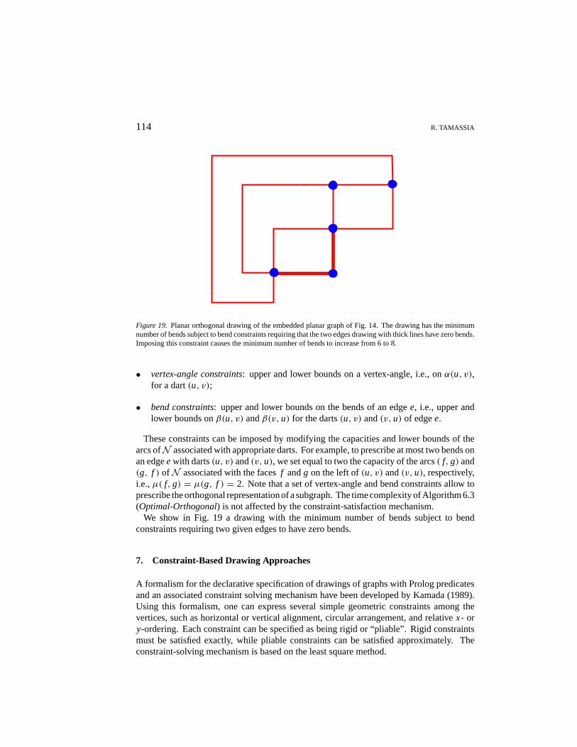
Figure 19. Planar orthogonal drawing of the embedded planar graph of Fig. 14. The drawing has the minimumnumber of bends subject to bend constraints requiring that the two edges drawing with thick lines have zero bends.Imposing this constraint causes the minimum number of bends to increase from 6 to 8.

• vertex-angle constraints: upper and lower bounds on a vertex-angle, i.e., onα(u, v),for a dart(u, v);

• bend constraints: upper and lower bounds on the bends of an edgee, i.e., upper andlower bounds onβ(u, v) andβ(v, u) for the darts(u, v) and(v, u) of edgee.

These constraints can be imposed by modifying the capacities and lower bounds of thearcs ofN associated with appropriate darts. For example, to prescribe at most two bends onan edgeewith darts(u, v) and(v, u), we set equal to two the capacity of the arcs( f, g) and(g, f ) ofN associated with the facesf andg on the left of(u, v) and(v, u), respectively,i.e.,µ( f, g) = µ(g, f ) = 2. Note that a set of vertex-angle and bend constraints allow toprescribe the orthogonal representation of a subgraph. The time complexity of Algorithm 6.3(Optimal-Orthogonal) is not affected by the constraint-satisfaction mechanism.

We show in Fig. 19 a drawing with the minimum number of bends subject to bendconstraints requiring two given edges to have zero bends.

7. Constraint-Based Drawing Approaches

A formalism for the declarative specification of drawings of graphs with Prolog predicatesand an associated constraint solving mechanism have been developed by Kamada (1989).Using this formalism, one can express several simple geometric constraints among thevertices, such as horizontal or vertical alignment, circular arrangement, and relativex- ory-ordering. Each constraint can be specified as being rigid or “pliable”. Rigid constraintsmust be satisfied exactly, while pliable constraints can be satisfied approximately. Theconstraint-solving mechanism is based on the least square method.


Dengler, Friedell, and Marks (1993), Kosak, Marks, and Shieber (1994), Marks (1991)provide a notation for describing the desired perceptual organization of a layout of a graphby means of a collection of layout patterns calledvisual organization features, which includeclustering, zoning, sequential placement, T shape, and hub shape. They also present threemethods that take as input a graph and a set of visual organization features, and producean aesthetically pleasing drawing that exhibits the specified visual organization features.The first method is rule-based and implemented in Prolog. The second method is a geneticalgorithm to be executed by a massively parallel computer. The third, method (Dengler,Friedell, and Marks, 1993) incrementally improves an initial randomly-generated drawingusing a force-directed technique, and is the most practical. This approach has also beenused within an interactive graph drawing system (Ryall, Marks, and Shieber, 1997).

Luders et al. (1995) present a combinatorial approach for satisfying inequality constraintsbetween vertex coordinates within a graph drawing system. Kamps et al. (1996) show howto extend force-directed methods to support the following geometric constraints: fixedvertex positions, fixed distances between pairs of vertices, relativex- or y-ordering, andhorizontal or vertical alignment.

A comprehensive approach to constrained graph drawing is presented by He and Marriott(1997). They give a general model that supports:

• the specification of arbitrary arithmetic linear equality and inequality constraints on thecoordinates of the vertices; and

• suggested coordinates for the vertices, each with an associated weight, which denotesthe strength of the suggestion.

They show how to extend the force-directed approach by Kamada and Kawai (1989) tosupport such constraints using a technique based on the “active set method” that is fastand gives good results in practice. They also present a simplified approach for constraineddrawings of rooted trees.

In related work, Eades and Lin (1995) attempt at combining algorithmic and constraint-based declarative methods in drawings of trees, and Brandenburg presents a comprehensiveapproach to graph drawing based on graph grammars (Brandenburg, 1995), where drawingsare generated by rule-based methods.

8. Visual Graph Drawing

A visual approach to graph drawing, where the layout of a graph is pictorially specified “byexample,” is proposed by Cruz and Garg (1995). Within this approach, a graph is storedin an object-oriented database, and its drawing is visually defined using recursive rules ofthe visual meta-languageDOODLE (Cruz, 1992). The application of the visual rules to theinput graph yields a system of constraints that can be solved in linear time for the followingtypes of drawings:

• layered drawings and box inclusion drawings of binary trees;

• 1-drawings of series-parallel digraphs (Bertolazzi et al., 1994);

116 R. TAMASSIA

VisibilityDrawing

v: sourceVertex

ORIGIN

F 0.5 [h]0.5 [h]

LE RE

F

f: face

F

VisibilityDrawing

e:edge

VisibilityDrawing

F

MW

F

MEmax ( 1, D) [h

,v]

RE

RE

MS

MN

left(e)right(e)

bot(e)

top(e)

left(v)

right(v)

VisibilityDrawing

v: vertex

F 0.5 [h]0.5 [h]

LE RE

Fleft(v)

right(v)

(a)

(b) (c)

(d)

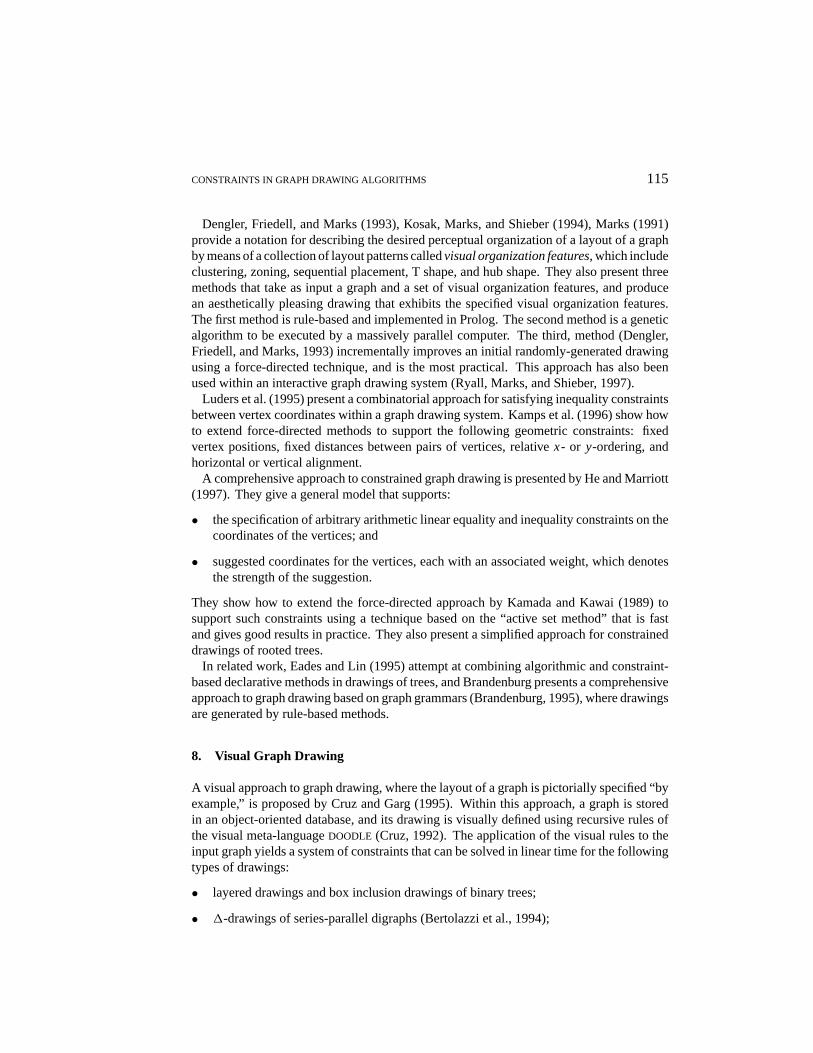
Figure 20. Visual rules for constructing a visibility representation of a planarst-digraph: (a) rule for a face;(b) special rule for the source vertex; (c) rule for a vertex; (d) rule for an edge.

• polyline drawings (Di Battista and Tamassia, 1988), visibility drawings (Tamassia andTollis, 1986), and tessellation drawings (Tamassia and Tollis, 1989) of upward planardigraphs.

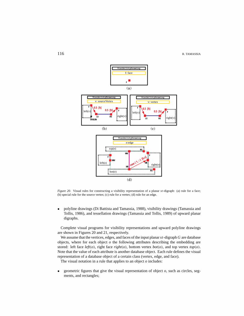
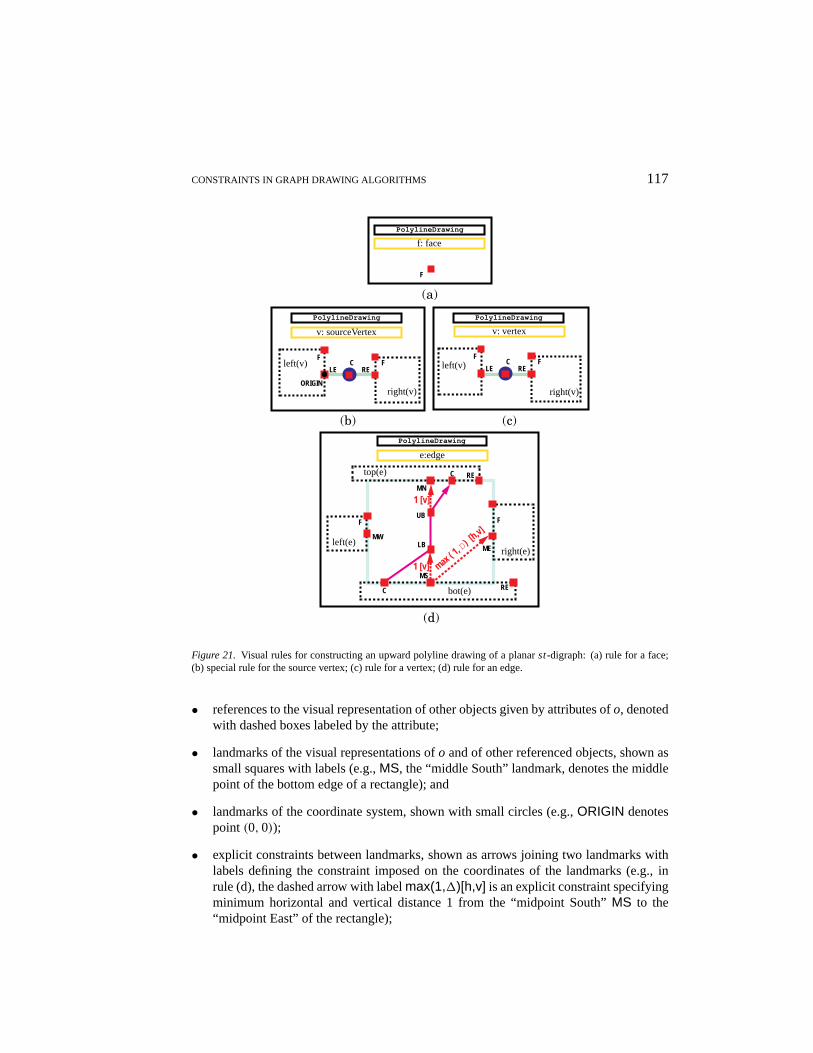
Complete visual programs for visibility representations and upward polyline drawingsare shown in Figures 20 and 21, respectively.

We assume that the vertices, edges, and faces of the input planarst-digraphG are databaseobjects, where for each objecto the following attributes describing the embedding arestored: left faceleft(o), right faceright(o), bottom vertexbot(o), and top vertextop(o).Note that the value of each attribute is another database object. Each rule defines the visualrepresentation of a database object of a certain class (vertex, edge, and face).

The visual notation in a rule that applies to an objecto includes:

• geometric figures that give the visual representation of objecto, such as circles, seg-ments, and rectangles;


(a)

(b) (c)

(d)

F

LEF

RE

ORIGIN

C

PolylineDrawing

F

LEF

REC

v: sourceVertex

left(v)

right(v)

v: vertex

left(v)

right(v)

PolylineDrawing

f: face

F

PolylineDrawing

e:edge

F

MW

F

ME

max ( 1, D

) [h,v]

RE

RE

MS

MN

left(e)right(e)

bot(e)

top(e)

PolylineDrawing

1 [v]

1 [v]

LB

UB

C

C

Figure 21. Visual rules for constructing an upward polyline drawing of a planarst-digraph: (a) rule for a face;(b) special rule for the source vertex; (c) rule for a vertex; (d) rule for an edge.

• references to the visual representation of other objects given by attributes ofo, denotedwith dashed boxes labeled by the attribute;

• landmarks of the visual representations ofo and of other referenced objects, shown assmall squares with labels (e.g.,MS, the “middle South” landmark, denotes the middlepoint of the bottom edge of a rectangle); and

• landmarks of the coordinate system, shown with small circles (e.g.,ORIGIN denotespoint (0, 0));

• explicit constraints between landmarks, shown as arrows joining two landmarks withlabels defining the constraint imposed on the coordinates of the landmarks (e.g., inrule (d), the dashed arrow with labelmax(1,1)[h,v] is an explicit constraint specifyingminimum horizontal and vertical distance 1 from the “midpoint South”MS to the“midpoint East” of the rectangle);

118 R. TAMASSIA

• implicit constraints between landmarks, given by their horizontal or vertical alignment(e.g., in rule (d), the “midpoint East”ME of the rectangle associated with edgeeand the“top endpoint”TE of the referenced visual representation of the right face ofe right(e)must have the samex-coordinate because they are drawn vertically aligned).

In these two programs, the visual representation of the faces is a single point associatedwith landmarkF, which is invisible but contributes to the definition of the constraints.Also, the visual representation of an edge includes a visible portion (vertical segment fora visibility representation and polygonal chain with three segments for an upward polylinedrawing) and an invisible portion drawn with a conventional “transparent color” (a rectangleor segment with shaded lines in the figures).

9. Conclusions

Because of the importance of constraint satisfaction in practical graph visualization ap-plications, the study of constraints is a strategic research direction for the graph drawingfield.

In this paper, we have overviewed fundamental algorithmic techniques for drawing graphs,and we have shown how they can be extended to support a limited constraint satisfactioncapability. The force-directed drawing approach appears to be the most suited for thesatisfaction of geometric constraints, while topological and shape constraints seem to bebetter handled by techniques based on planarization and network flow. We have also men-tioned methods for the specification of constraints and declarative rule-based approachesfor constraint resolution.

10. Acknowledgment

I would like to thank Ioannis G. Tollis for useful comments.

References

R. K. Ahuja, T. L. Magnanti, & J. B. Orlin. (1993).Network Flows: Theory, Algorithms, and Applications.Prentice Hall, Englewood Cliffs, NJ.

P. Bertolazzi, R. F. Cohen, G. Di Battista, R. Tamassia, & I. G. Tollis. (1994). How to draw a series-paralleldigraph.Internat. J. Comput. Geom. Appl. 4: 385–402.

F. J. Brandenburg. (1995). Designing graph drawings by layout graph grammars. In R. Tamassia and I. G. Tollis(eds.),Graph Drawing (Proc. GD ’94), volume 894 ofLecture Notes Comput. Sci., pages 416–427. Springer-Verlag.

F. J. Brandenburg, M. Himsolt, & C. Rohrer. (1996). An experimental comparison of force-directed and random-ized graph drawing algorithms. In F. J. Brandenburg (ed.),Graph Drawing (Proc. GD ’95), volume 1027 ofLecture Notes Comput. Sci., pages 76–87. Springer-Verlag.

I. F. Cruz. (1992) DOODLE: A visual language for object-oriented databases. InProc. ACM SIGMOD, pages 71–80.

I. F. Cruz & A. Garg. (1995). Drawing graphs by example efficiently: Trees and planar acyclic digraphs. InR. Tamassia and I. G. Tollis (eds.),Graph Drawing (Proc. GD ’94), volume 894 ofLecture Notes Comput. Sci.,pages 404–415. Springer-Verlag.


R. Davidson & D. Harel. (1996). Drawing graphics nicely using simulated annealing.ACM Trans. Graph. 15(4):301–331.

E. Dengler, M. Friedell, & J. Marks. (1993). Constraint-driven diagram layout. InProc. IEEE Sympos. on VisualLanguages, pages 330–335.

G. Di Battista, P. Eades, R. Tamassia, & I. G. Tollis. (1994). Algorithms for drawing graphs: An annotatedbibliography.Comput. Geom. Theory Appl. 4: 235–282.

G. Di Battista & R. Tamassia. (1988). Algorithms for plane representations of acyclic digraphs.Theoret. Comput.Sci. 61: 175–198.

G. Di Battista, R. Tamassia, & I. G. Tollis. (1992). Constrained visibility representations of graphs.Inform.Process. Lett. 41: 1–7.

P. Eades. (1984). A heuristic for graph drawing.Congr. Numer. 42: 149–160.S. Even. (1979).Graph Algorithms. Computer Science Press, Potomac, Maryland.A. Frick, A. Ludwig, & H. Mehldau. (1995). A fast adaptive layout algorithm for undirected graphs. In

R. Tamassia and I. G. Tollis (eds.),Graph Drawing (Proc. GD ’94), volume 894 ofLecture Notes Comput. Sci.,pages 388–403. Springer-Verlag.

T. Fruchterman & E. Reingold. (1991). Graph drawing by force-directed placement.Softw. – Pract. Exp. 21(11):1129–1164.

M. R. Garey & D. S. Johnson. (1983). Crossing number is NP-complete.SIAM J. Algebraic Discrete Methods4(3): 312–316.

A. Garg & R. Tamassia. (1997). A new minimum cost flow algorithm with applications to graph drawing. InS. North (ed.),Graph Drawing (Proc. GD ’96), volume 1190 ofLecture Notes Comput. Sci., pages 201–216.Springer-Verlag.

A. Gibbons. (1980).Algorithmic Graph Theory. Cambridge University Press, Cambridge.D. Harel & M. Sardas. (1995). Randomized graph drawing with heavy-duty preprocessing.J. Visual Lang.

Comput. 6(3). (Special issue on Graph Visualization, edited by I. F. Cruz and P. Eades.)W. He & K. Marriott. (1997). Constrained graph layout. In S. North (ed.),Graph Drawing (Proc. GD ’96),

volume 1190 ofLecture Notes Comput. Sci., pages 217–232. Springer-Verlag.M. Junger & P. Mutzel. (1996). Maximum planar subgraphs and nice embeddings: Practical layout tools.

Algorithmica16(1). (Special issue on Graph Drawing, edited by G. Di Battista and R. Tamassia.)T. Kamada. (1989).Visualizing Abstract Objects and Relations. World Scientific Series in Computer Science.T. Kamada & S. Kawai. (1989). An algorithm for drawing general undirected graphs.Inform. Process. Lett. 31:

7–15.T. Kamps, J. Kleinz, & J. Read. (1996). Constraint-based spring-model algorithm for graph layout. In F. J. Bran-

denburg (ed.),Graph Drawing (Proc. GD ’95), volume 1027 ofLecture Notes Comput. Sci., pages 349–360.Springer-Verlag.

C. Kosak, J. Marks, & S. Shieber. (1994). Automating the layout of network diagrams with specified visualorganization.IEEE Trans. Syst. Man Cybern. 24(3): 440–454.

J. B. Kruskal & J. B. Seery. (1980). Designing network diagrams. InProc. First General Conference on SocialGraphics, pages 22–50. U.S. Department of the Census.

T. Lin & P. Eades. (1995). Integration of declarative and algorithmic approaches for layout creation. In R. Tamassia& I. G. Tollis (eds.),Graph Drawing (Proc. GD ’94), volume 894 ofLecture Notes Comput. Sci., pages 376–387.Springer-Verlag.

P. Luders, R. Ernst, & S. Stille. (1995). An approach to automatic display layout using combinatorial optimization.Software-Practice and Experience25(11): 1183–1202.

J. Marks. (1991). A formal specification for network diagrams that facilitates automated design.J. Visual Lang.Comput. 2: 395–414.

K. Mehlhorn. (1984).Data Structures and Algorithms. Volumes 1–3. Springer-Verlag.T. Nishizeki & N. Chiba. (1988). Planar graphs: Theory and algorithms.Ann. Discrete Math. 32.P. Rosenstiehl & R. E. Tarjan. (1986). Rectilinear planar layouts and bipolar orientations of planar graphs.

Discrete Comput. Geom. 1(4): 343–353.K. Ryall, J. Marks, & S. Shieber. (1997). An interactive system for drawing graphs. In S. North (ed.),Graph

Drawing (Proc. GD ’96), volume 1190 ofLecture Notes Comput. Sci., pages 387–393. Springer-Verlag.K. Sugiyama & K. Misue. (1995). Graph drawing by magnetic-spring model.J. Visual Lang. Comput. 6(3).

(Special issue on Graph Visualization, edited by I. F. Cruz and P. Eades.)R. Tamassia. (1985). New layout techniques for entity-relationship diagrams. InProc. 4th Internat. Conf. on

Entity-Relationship Approach, pages 304–311.

120 R. TAMASSIA

R. Tamassia. (1987). On embedding a graph in the grid with the minimum number of bends.SIAM J. Comput.16(3): 421–444.

R. Tamassia. (1997). Graph drawing. In J. E. Goodman & J. O’Rourke (eds.),CRC Handbook of Discrete andComputational Geometry. CRC Press.

R. Tamassia, G. Di Battista, & C. Batini. (1988). Automatic graph drawing and readability of diagrams.IEEETrans. Syst. Man Cybern. SMC-18(1): 61–79.

R. Tamassia & I. G. Tollis. (1986). A unified approach to visibility representations of planar graphs.DiscreteComput. Geom. 1(4): 321–341.

R. Tamassia & I. G. Tollis. (1989). Tessellation representations of planar graphs. InProc. 27th Allerton Conf.Commun. Control Comput., pages 48–57.

W. T. Tutte. (1960). Convex representations of graphs.Proceedings London Mathematical Society10(3): 304–320.

W. T. Tutte. (1963). How to draw a graph.Proceedings London Mathematical Society13(3): 743–768.

Date post:	22-Jun-2020
Category:	Documents
Upload:	others
View:	42 times
Download:	2 times

Constraints in Graph Drawing...

Documents