Constructing lower-bounds for CTL escape rates in early SIV infection

Sivan LeviyangGeorgetown University, Department of Mathematics and Statistics, United States

H I G H L I G H T S

� In HIV and SIV infections, the viral population repeatedly escapes from CTL response.� We develop inference methods to estimate the rate of the first CTL escape.� Using frequency data, we construct estimators which serve as lower bounds for the escape rate.� The early part of the first CTL escape proceeds quicker than later parts.� The rate of the first CTL escape diers across dierent infected compartments.

a r t i c l e i n f o

Article history:Received 30 July 2013Received in revised form15 January 2014Accepted 17 February 2014Available online 3 March 2014

Keywords:CTL escapeEscape rateSIVHIV

a b s t r a c t

Intrahost human and simian immunodeficiency virus (HIV and SIV) evolution is marked by repeated viralescape from cytotoxic T-lymphocyte (CTL) response. Typically, the first such CTL escape starts around thetime of peak viral load and completes within one or two weeks. Many authors have developed methodsto quantify CTL escape rates, but existing methods depend on sampling at two or more timepoints. Sincemany datasets capture the dynamics of the first CTL escape at a single timepoint, we develop inferencemethods applicable to single timepoint datasets. To account for model uncertainty, we constructestimators which serve as lower bounds for the escape rate. These lower-bound estimators allow forstatistically meaningful comparison of escape rates across different times and different compartments.We apply our methods to two SIV datasets, showing that escape rates are relatively high during the initialdays of the first CTL escape and drop to lower levels as the escape proceeds.

& 2014 Elsevier Ltd. All rights reserved.

1. Introduction

During HIV and SIV infections, the viral population repeatedlyescapes from selective pressure exerted by cytotoxic T-lymphocytes(CTLs), a type of immune system cell. Each CTL targets a specificpeptide, referred to as an epitope, associated with a locus on theviral genome. Mutation at the locus may change the epitope,making it partially or completely unrecognisable by existing CTLs.Viruses possessing such mutations are at a selective advantage,leading to a selective sweep referred to as a CTL escape. See Goulderand Watkins (2004) for a review of CTL escape in both HIV and SIVinfections.

In this work, we consider the first CTL escape to occur duringan infection. In SIV and HIV infections, CTL response initiatesroughly at 14 and 21 days after infection, respectively, just prior topeak viral load (Borrow et al., 1994; Cohen et al., 2011; Goulderand Watkins, 2004; McMichael et al., 2010). In the week or twofollowing the initiation of CTL response, CTL escape often occurs ata single targeted epitope (Boutwell et al., 2010; McMichael et al., 2010;Goonetilleke et al., 2009; Henn et al., 2012; Allen et al., 2000). T-cell

tetramer studies suggest that this escape is driven by an especiallyfocused CTL response in comparison to subsequent responses andescapes (Turnbull et al., 2009; Yasutomi et al., 1994; Veazey et al.,2003).

Many authors have attempted to quantify the strength of CTLresponse by measuring the rate at which CTL escape occurs.A commonly used method (e.g. Goonetilleke et al., 2009; Love et al.,2008; Loh et al., 2008; Asquith and McLean, 2007; Ganusov et al.,2011), introduced in Fernandez et al. (2005), Asquith et al. (2006), fitsescape mutation frequencies at two timepoints to a differentialequation model. The model fit is determined by a parameter, knownas the escape rate, which is used to quantify the strength of CTLresponse at a given epitope. Since this approach requires frequencydata at two timepoints, we call it the two-point method.

Using the two-point method to analyze the first CTL escape isdifficult because rarely do both sampled timepoints capture theescape. For example, the first two timepoints available in HIVstudies of acute infection are typically in the range of days 30 and50, e.g. Fisher et al. (2010) and Goonetilleke et al. (2009). Using thetwo-point method on such data estimates escape rates between

Contents lists available at ScienceDirect

journal homepage: www.elsevier.com/locate/yjtbi

Journal of Theoretical Biology

http://dx.doi.org/10.1016/j.jtbi.2014.02.0200022-5193 & 2014 Elsevier Ltd. All rights reserved.

Journal of Theoretical Biology 352 (2014) 82–91

days 30 and 50, while CTL response is likely strongest prior to day30. The situation is different for SIV studies. Since the time ofinfection can be controlled, sampling timepoints can be chosenthat straddle day 14, the approximate time of CTL response; forexample sampling can occur at days 7 and 21. But usually the CTLescape has not started at day 7, so the two-point method must beapplied using data collected at day 21 and a later timepoint,leading to the same difficulties seen in HIV datasets.

Other authors (e.g. Mandl et al., 2007; Althaus and de Boer,2008; Petravic et al., 2008; Monteiro et al., 2000) have developedmethods based on the standard model of viral dynamics (Perelson,2002; Nowak and May, 2000). These methods depend on modelswith many parameters, in contrast the two-point method dependsonly on the escape rate and the mutation frequencies at the twotimepoints. Further, fitting the standard model and its variantsrequires multiple timepoints, so the time period to which suchescape rate estimates apply is often unclear. Recently, haplotypedata has been used to estimate escape rates, but this method ismore applicable to later timepoints in infection, when the viralpopulation possesses significant genetic diversity (Messer andNeher, 2012).

The rate of CTL escape can be defined in different ways. Forexample, some authors measure the timespan from initiation ofCTL response to the time when mutant frequencies reach aprescribed level (Liu et al., 2006; Palmer et al., 2013). In the two-point method, using the underlying model, the escape rate is thedifference between the average CTL kill rate and the fitness cost ofmutation (Asquith et al., 2006; Fernandez et al., 2005). We takethis as our definition of the escape rate.

In this work, we develop inference methods for estimating therate of the first CTL escape using frequency data from a singletimepoint. We apply these methods to SIV datasets, a setting inwhich inference is slightly easier because infection time is typi-cally known, but our methods extend to HIV escape as well. ForSIV infection, we have in mind frequency data collected some-where between days 14 and 28, times that capture the first CTLescape when the mutation frequency is substantial, but beforeescape at other epitopes has developed. Single timepoint methodshave been used to infer early growth rates for cytomegalovirus, asituation in which immune response and viral mutation are lessimportant (Cromer et al., 2013).

The price we pay for using a single timepoint is the need for anunderlying model describing viral dynamics and evolution in theearly stages of infection, prior to peak viral load. Specifying such amodel is difficult because the dynamics of early SIV and HIVinfections are poorly understood. We solve this difficulty byintroducing a model that allows for a range of assumptions onearly viral dynamics depending on the parameters chosen. Then,in order to cope with the resulting large parameter space, wederive estimators which serve as lower bounds for the escape rateover a large range of possible models.

We apply our methods to the two SIV datasets presented inBimber et al. (2009) and Vanderford et al. (2011). By combininglower-bound estimators and the two-point method, we are able tocompare escape rates between early and late time periods duringthe first CTL escape, as well as across different compartments. Ourresults also clarify the role of different modeling assumptions onescape rate inference.

2. Results

2.1. Model

Our model distinguishes between two types of infected cells:wild type and mutant. Wild types contain the epitope at which the

first CTL escape occurs; mutants contain a nucleotide mutation atthat epitope. w(t) and m(t) represent the number of wild type andmutant type, respectively, at t days post infection. f(t) representsthe mutant frequency at t, i.e. f ðtÞ ¼mðtÞ=ðwðtÞþmðtÞÞ.

The model depends on the seven parameters listed in Table 1.To start, we present the model assuming no mutation-associatedfitness costs; c¼0. The parameter tA specifies the time, in units ofdays post infection, when CTL response initiates. Specification ofthe model splits according to whether times are before of after tA.

For times prior to tA, wild type dynamics are specified throughthe parameter r(t) and the equation

dwdt

ðtÞ ¼ rðtÞwðtÞ: ð1Þ

r(t) is the wild type growth rate in units of day�1. By choosing r(t)appropriately, arbitrary profiles for w(t) are possible, reflecting theflexibility of the model.

Given w(t), the parameters μ and XðtA; sÞ specify the distribu-tion of mðtAÞ through the equation

mðtAÞ ¼ ∑N

i ¼ 1XðtA; siÞ: ð2Þ

The si for i¼ 1;2;…;N are the times prior to tA at which a wild typemutated. The si are stochastic and are generated at a non-constantrate μwðsÞ. XðtA; sÞ, termed the offspring distribution, gives thenumber of mutants at time tA that descend from a wild typeinfected cell which mutated at time s. Importantly, XðtA; sÞ is arandom variable. When no fitness costs exist, we assume

E½XðtA; sÞ� ¼ expZ tA

srðs0Þ ds0

� �; ð3Þ

so that mutants have the same average growth rate as wild types.In (3), exp½x� represents the exponential taken to the power of x,i.e. ex, and E½� denotes the expected value.

To explain XðtA; sÞ more concretely, we provide three examples:

X1ðtA; sÞ ¼ expZ tA

srðs0Þ ds0

� �; ð4Þ

X2ðtA; sÞ ¼ 2nBernoullið:5ÞnexpZ tA

srðsÞ ds

� �; ð5Þ

X3ðtA; sÞ ¼H=2nexpZ tA

srðsÞ ds

� �: ð6Þ

Above, Bernoulli(.5) is a Bernoulli random variable with successprobability .5 and H is a continuous distribution on ½1;1Þ withdensity 2=y3, a heavy tailed distribution. All three XiðtA; sÞ satisfyE½XiðtA; sÞ� ¼ exp½R tAs rðs0Þ ds0�, however, the variance increases fromzero for X1ðtA; sÞ to infinity for X3ðtA; sÞ. Little is known about theform of XðtA; sÞ in SIV and HIV infections, but experimental resultssuggesting that HIV has an effective population size much smallerthan its census size could correspond to offspring distributions

Table 1Model parameters.

Parameter Description Units

tA CTL response time daytF Sampling time dayμ Epitope mutation rate mutant infected cell

day �wild type infected cellr(t) Wild type growth rate day�1

k(t) CTL kill rate day�1

XðtA; sÞ Offspring distribution infected cellsc Fitness cost day�1

S. Leviyang / Journal of Theoretical Biology 352 (2014) 82–91 83

such as X2ðtA; sÞ or X3ðtA; sÞ (Kouyos et al., 2006; Leigh-Brown,1997).

For times after tA, we switch to a deterministic model. In thedatasets considered below, CTL response arises one or two daysprior to or just at peak viral load. As discussed below, f ðtAÞ � μtA,leading to m(t) in the 100 s or greater. As several authors havenoted, when mutant population size reaches such values, aver-aging effects reduce the impact of stochasticity and the dynamicsbecome deterministic, see Rouzine and Coffin (2005), Kessingeret al. (2013), Leviyang (2013) and Desai and Fisher (2007). Thestochastic model could be extended past tA in cases for whichmðtAÞ is modest, see Section 3.

After tA, we model w(t) and m(t) through the equations

dwdt

ðtÞ ¼ ðrðtÞ�kðtÞÞwðtÞ;

dmdt

ðtÞ ¼ rðtÞmðtÞþμwðtÞ; ð7Þ

where k(t) is the CTL-mediated killing rate of wild type infectedcells between times tA and tF in units of day�1, see Ganusov et al.(2013) for a similar model. (7) can be recast in terms of the mutantfrequency f(t) to give

dfdt

ðtÞ ¼ μð1� f ðtÞÞþðkðtÞ�μÞf ðtÞð1� f ðtÞÞ: ð8Þ

To model a fitness cost c, we change (8) to

dfdt

ðtÞ ¼ μð1� f ðtÞÞþðkðtÞ�c�μÞf ðtÞð1� f ðtÞÞ; ð9Þ

and (3) to

E½XðtA; sÞ� ¼ expZ tA

sðrðsÞ�cÞ ds

� �: ð10Þ

2.2. Inference methods

Let f̂ data be the estimate of mutant frequency obtained bysampling viral sequences at time tF. Using f̂ data, our goal is to inferthe escape rate k�c, where k is the average kill rate between tAand tF

k ¼ 1tF�tA

Z tF

tAkðsÞ ds;

and c is the mutation-associated fitness cost. To start, we assumeno fitness costs, i.e. c¼0, and present three estimators of k, kD, kG

and kR, referred to as the deterministic, general, and restrictedestimator, respectively. kG and kR serve as lower bounds for k.Towards the end of the section we consider fitness costs, showingthat kG and kR are lower bounds for k�c.

Regardless of the estimator, our approach involves the samesteps. We assume that the parameters μ; tA; tF are known andbased on these parameters, we select a value for f ðtAÞ, labeledf̂ silico, and a family of profiles kðt; kÞ. For every possible value of k,kðt; kÞ is a specific CTL kill rate profile with average k. Then,starting (8) at time tA with f ðtAÞ ¼ f̂ silico, we fit k by integrating (8)to time tF and selecting the k satisfying f ðtF Þ ¼ f̂ data. The distinctionbetween the three estimators lies in the choice for f̂ silico and thefamily kðt; kÞ.

To construct kD, we take a deterministic approach, using (8) tocompute f ðtAÞ. Setting f ð0Þ ¼ 0 and integrating (8) to tA withkðtÞ ¼ 0 gives f ðtAÞ ¼ μtA and so we set f̂ silico ¼ μtA. Equivalently,f̂ silico ¼ E½f ðtAÞ� since (8) gives the mean dynamics of f(t), as can beseen by taking the expected value of (2). To build kðt; kÞ, weassume that CTL kill rates are constant once CTL response begins,making kðt; kÞ ¼ k for tA ½tA; tF �.

Given these choices for f̂ silico and kðt; kÞ, kD satisfies therelation:

f̂ data ¼1

1þ exp½�kDðtF�tAÞ�μtAþ

μkD

ð1�exp½�kDðtF�tAÞ�Þ

: ð11Þ

If we ignore mutations occurring after tA, the two-point methodwith f ðtAÞ ¼ μtA and f ðtF Þ ¼ f̂ data can be applied, leading to thefollowing approximation:

kD � 1tF�tA

logf̂ data

ð1� f̂ dataÞμtA

!: ð12Þ

As we show below through numerical experiments, kD is auseful estimator. However, kD often overestimates k and we wouldlike estimators which serve as lower bounds for k in order tocompare escape rates across different times and compartments.To develop an estimator which is less than k with confidence 1�s,we choose f̂ silico so that f ðtAÞo f̂ silico with probability at least 1�sacross a range of parametrizations. To choose kðt; kÞ, we selectprofiles maximizing the number of mutations occurring after tAgiven fixed values of f ðtAÞ and k. Overestimating f ðtAÞ through f̂ silicoand maximizing the number of mutations after tA, leads tounderestimates of k because less CLT-mediated killing is necessaryto achieve f ðtF Þ ¼ f̂ data. See Section 3 for more details. As a result,under a null model in which f̂ data is generated according to thestochastic model with k as the average for the k(t) parameterchosen, estimators constructed in this manner will be less than kwith probability at least 1�s.

To construct kG we set f̂ silico ¼ μtA=s. For the kðt; kÞ profiles seeSection 3, but roughly we choose profiles which delay most of thekilling until time tF. Intuitively, delaying killing allows moremutations to occur after time tA, thereby raising f ðtF Þ. kG satisfiesthe relation

f̂ data ¼1

1þexp½�kGðtF�tAÞ�μtAs þμðtF�tAÞ

; ð13Þ

which can be solved to find

kG ¼ 1tF�tA

logf̂ data

μtAs þμðtF�tAÞ

0B@

1CA: ð14Þ

kG is often a poor lower bound; in many cases, it significantlyunderestimates k. The poor behaviour derives from the largeparameter space, namely all choices for rðtÞ; kðtÞ;XðtA; sÞ. To pro-duce a better lower-bound estimator, we consider smaller para-meter spaces by requiring rðtÞZrmin for totA and k″ðtÞo0, wherermin ¼ :8. XðtA; sÞ is allowed to take any value. The restrictionrðtÞZrmin assumes a minimum expansion rate for the number ofinfected cells prior to CTL response time tA. k″ðtÞo0 assumes CTLkill rates rise quickest at the beginning of the CTL response. Otherrestrictions are possible, reflecting different biological assump-tions. Assuming these restrictions, kR is constructed usingf̂ silico ¼ μtAð1þ2=ðrmin tAsÞÞ and kðt; kÞ ¼ 2kðt�tAÞ=ðtF�tAÞ, a line-arly increasing profile. kR satisfies the relation

f̂ data ¼1

1þ exp½�kRðtF�tAÞ�μtA 1þ 2

stArmin

� �þμ

ffiffiffiffiffiffiffiffiffiffiffiffiffiπðtF�tAÞ

4kR

q: ð15Þ

S. Leviyang / Journal of Theoretical Biology 352 (2014) 82–9184

Ignoring mutations after tA allows the two-point method to beapplied giving the approximation,

kR �1

tF�tAlog

f̂ data

ð1� f̂ dataÞμtA 1þ 2stArmin

� �0BB@

1CCA: ð16Þ

Now we consider the presence of a fitness cost c. kG and kR areconstructed assuming no fitness costs, but the two estimators arelower-bounds for the escape rate when fitness costs exist. BetweentA and tF, introducing a fitness cost can be seen as a shift of k(t) tokðtÞ�c. Correspondingly, kG and kR shift from lower bounds for kto lower bounds for k�c. f̂ silico is still an upper bound for f ðtA)because fitness costs reduce f ðtAÞ, meaning that the probabilityf̂ silico is greater than f ðtAÞ will increase. As a result, kG and kR arelower-bounds for the escape rate in the absence or presence offitness costs.

In practice, μ and tA are unknown, but are needed for all threeestimation methods. Using the approximate formulas for the threeestimators and letting tF�tA ¼ 7, we calculate that mistaking μ bya factor of 10 shifts all estimators by roughly :3. The estimators areshifted down as μ is increased, so to maintain the lower-bounds μshould be overestimated. As discussed in Mandl et al. (2007),assuming an epitope composed of roughly 30 nucleotides, amutation rate of 3�10�5 per base pairing (Mansky, 1996), andabout 2/3 of mutations being non-synonymous, leads to anepitope mutation rate of μ¼ 6� 10�4 which is likely greater thanthe true rate.

If the parameter tA is less than the true tA value, then the truek(t) will be zero for times greater than the parameter tA but lessthan the true tA. There is nothing in the model and estimators thatprohibit this, except that the restriction k″ðtÞ40 for kR will nothold. In contrast, using a tA value greater than the true tA value willbias the estimators up because more mutants will exist at tA thenpredicted under the model. To preserve lower-bounds, tetramerdata should be used to estimate tA, with underestimation preferredto overestimation.

2.3. Numerical experiments

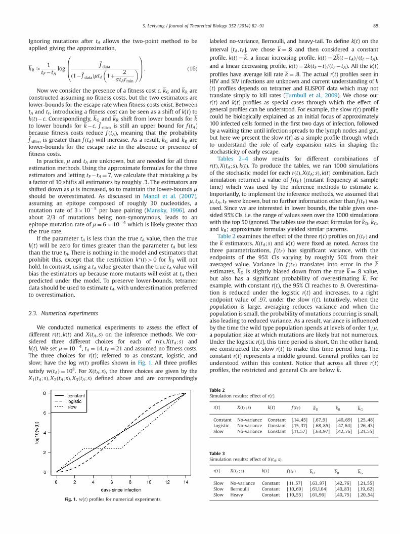
We conducted numerical experiments to assess the effect ofdifferent rðtÞ; kðtÞ and XðtA; sÞ on the inference methods. We con-sidered three different choices for each of rðtÞ;XðtA; sÞ andk(t). We set μ¼ 10�4, tA ¼ 14; tF ¼ 21 and assumed no fitness costs.The three choices for r(t); referred to as constant, logistic, andslow; have the log wðtÞ profiles shown in Fig. 1. All three profiles

satisfy wðtAÞ ¼ 108. For XðtA; sÞ, the three choices are given by theX1ðtA; sÞ;X2ðtA; sÞ;X3ðtA; sÞ defined above and are correspondingly

labeled no-variance, Bernoulli, and heavy-tail. To define k(t) on the

interval ½tA; tF �, we chose k ¼ :8 and then considered a constant

profile, kðtÞ ¼ k, a linear increasing profile, kðtÞ ¼ 2kðt�tAÞ=ðtF�tAÞ,and a linear decreasing profile, kðtÞ ¼ 2kðtF�tÞ=ðtF�tAÞ. All the k(t)

profiles have average kill rate k ¼ :8. The actual r(t) profiles seen inHIV and SIV infections are unknown and current understanding of k(t) profiles depends on tetramer and ELISPOT data which may nottranslate simply to kill rates (Turnbull et al., 2009). We chose ourr(t) and k(t) profiles as special cases through which the effect ofgeneral profiles can be understood. For example, the slow r(t) profilecould be biologically explained as an initial focus of approximately100 infected cells formed in the first two days of infection, followedby a waiting time until infection spreads to the lymph nodes and gut,but here we present the slow r(t) as a simple profile through whichto understand the role of early expansion rates in shaping thestochasticity of early escape.

Tables 2–4 show results for different combinations ofrðtÞ;XðtA; sÞ; kðtÞ. To produce the tables, we ran 1000 simulationsof the stochastic model for each rðtÞ;XðtA; sÞ; kðtÞ combination. Eachsimulation returned a value of f ðtF Þ (mutant frequency at sampletime) which was used by the inference methods to estimate k.Importantly, to implement the inference methods, we assumed thatμ; tA; tF were known, but no further information other than f ðtF Þwasused. Since we are interested in lower bounds, the table gives one-sided 95% CIs, i.e. the range of values seen over the 1000 simulationswith the top 50 ignored. The tables use the exact formulas for kD, kG,and kR; approximate formulas yielded similar patterns.

Table 2 examines the effect of the three r(t) profiles on f ðtF Þ andthe k estimators. XðtA; sÞ and k(t) were fixed as noted. Across thethree parametrizations, f ðtF Þ has significant variance, with theendpoints of the 95% CIs varying by roughly 50% from theiraveraged value. Variance in f ðtF Þ translates into error in the kestimates. kD is slightly biased down from the true k ¼ :8 value,but also has a significant probability of overestimating k. Forexample, with constant r(t), the 95% CI reaches to .9. Overestima-tion is reduced under the logistic r(t) and increases, to a rightendpoint value of .97, under the slow r(t). Intuitively, when thepopulation is large, averaging reduces variance and when thepopulation is small, the probability of mutations occurring is small,also leading to reduced variance. As a result, variance is influencedby the time the wild type population spends at levels of order 1=μ,a population size at which mutations are likely but not numerous.Under the logistic r(t), this time period is short. On the other hand,we constructed the slow r(t) to make this time period long. Theconstant r(t) represents a middle ground. General profiles can beunderstood within this context. Notice that across all three r(t)profiles, the restricted and general CIs are below k.

Fig. 1. w(t) profiles for numerical experiments.

Table 2Simulation results: effect of r(t).

r(t) XðtA ; sÞ k(t) f ðtF Þ kD kR kG

Constant No-variance Constant [.14,.45] [.67,.9] [.46,.69] [.25,.48]Logistic No-variance Constant [.15,.37] [.68,.85] [.47,.64] [.26,.43]Slow No-variance Constant [.11,.57] [.63,.97] [.42,.76] [.21,.55]

Table 3Simulation results: effect of XðtA; sÞ.

r(t) XðtA; sÞ k(t) f ðtF Þ kD kR kG

Slow No-variance Constant [.11,.57] [.63,.97] [.42,.76] [.21,.55]Slow Bernoulli Constant [.10,.69] [.61,1.04] [.40,.83] [.19,.62]Slow Heavy Constant [.10,.55] [.61,.96] [.40,.75] [.20,.54]

S. Leviyang / Journal of Theoretical Biology 352 (2014) 82–91 85

Table 3 examines the effect of XðtA; sÞ. The Bernoulli XðtA; sÞincreases the variance of f ðtF Þ leading to wider CIs across all threeinference methods. Somewhat surprisingly, the heavy distributionleads to slightly less f ðtF Þ variance. While the heavy distributionallows for samples resulting in extremely high values of f ðtF Þ, suchsamples have small probability and their occurrence falls outsidethe 95% CI. Notice that, under a Bernoulli XðtA; sÞ and slow r(t), therestricted method's CI exceeds k ¼ :8, reflecting the erroneousassumption of rðtÞZrmin. In contrast, the general estimator's CIstays below k ¼ :8.

To understand the effect of k(t) on f ðtF Þ and the three estimators,

consider kD as defined through (11); the right hand side of (11) is f ðtF Þunder the assumptions f ðtAÞ ¼ f̂ silico ¼ μtA and kðt; kÞ ¼ kD. The

expressions μtA and μ=kDð1�exp½�kDðtF�tAÞ�Þ represent the con-tributions of mutations before and after tA, respectively, to f ðtF Þ. When

kDtA is large, the μtA term is dominant and f ðtF Þ is mostly influencedby mutations occurring prior to tA. Intuitively, a large kill rate pushesthe frequency of wild types down, reducing the number of mutationsoccurring after tA, and a large tA value increases the number ofmutations arising prior to tA. More generally, for arbitrary parame-

trizations of the stochastic model, as ktA increases, the profile of k(t)matters less to the value of f ðtF Þ. Consequently, numerical experiments

with k ¼ :8; tA ¼ 14; tF ¼ 21 show minor dependence on the k(t)profile (results not shown). In contrast, Table 4 shows simulation

results under k ¼ :2, tA ¼ 9; tF ¼ 35. The increasing and decreasing k(t)profiles produce more and less mutations after tA, respectively, withthe constant k(t) profile occupying a middle ground. As the resultsshow, producing more mutants after tA shifts all the CIs to the right. In

particular, under the increasing profile the kD CI is largely to the right

of the true k ¼ :2 value. Intuitively, the kD estimator underestimates

the number of mutations after tA, causing it to overestimate k. Notice

that kG and kR still serve as lower bounds.

2.4. Datasets

Most existing analyses of CTL escape infer a single rate for theentire escape. For the datasets below, we consider three times: tA,tF and tS. tA and tF are as previously defined, the CTL response timeand sampling time, but now we add a second sampling time tSsubsequent to tF. To tA and tF, we apply the discussed methods,estimating the escape rate between tA and tF. To tF and tS, we applythe two-point method, estimating the escape rate between tF andtS. Using the lower-bound estimators kG and kR, we investigatewhether escape rates from tA to tF are greater than escape ratesfrom tF to tS. In the case of the Vanderford et al. data, we alsocompare escape rates across compartments.

Given frequency data, our estimators and the two-point methodestimator provide point estimates for the escape rate. When samplingvariance associated with the data is included, the point estimatesgeneralize to CIs in a standardway. Conservatively, we assume that thefrequency data is accurate to roughly 10%, corresponding to 100 viralsequences at each timepoint. The CIs shown below are constructedaccordingly. In some of the following figures, sampling variance causesthe two-point method CIs to include negative escape rates. As anexample of how this might occur, suppose that the mutation frequen-cies provided by the data at times tF and tS are .4 and .45, respectively.Sampling variance allows the true mutation frequencies from whichthe data was sampled to be, say, .43 and .42, reflecting a drop inmutation frequency and a negative escape rate.

2.4.1. Bimber et al. datasetThe data from Bimber et al. involves four Mauritian cynomol-

gus macaques (MCMs) and four Rhesus macaques (RMs). (The fulldataset included eight RMs, we considered the four unvaccinatedRMs.) We refer the reader to the article and references therein forfull details (Bimber et al., 2009). Briefly, all animals were intrar-ectally infected with SIVmac239. The first CTL escape in the MCMswas at the epitope NEF-RM9, while CTL escape first occurred atTAT-SL8 in the RMs. Pyrosequencing of the epitopes was per-formed at various timepoints. At day 14 after infection, for both

Table 4Simulation results: effect of k(t).

r(t) XðtA; sÞ k(t) f ðtF Þ kD kR kG

Constant Constant Constant [.09,.29] [.16,.22] [.10,.16] [.06,.12]Constant Constant Decreasing [.05,.27] [.14,.22] [.08,.15] [.04,.11]Constant Constant Increasing [.16,.34] [.19,.23] [.13,.17] [.08,.12]

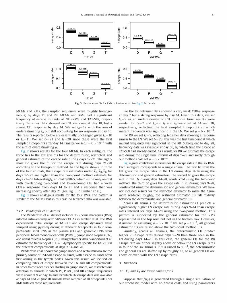
Fig. 2. Escape rates CIs for MCMs in Bimber et al. Each subfigure represents a single animal. Within each subfigure, the tics labeled D, R and G give escape rate CIs for days12–21 using, respectively, the deterministic, restricted, and general methods. The right tic gives the escape rate CI for days 21–28 as computed by the two-point method. AllCIs are at 95% significant and include sampling variance.

S. Leviyang / Journal of Theoretical Biology 352 (2014) 82–9186

MCMs and RMs, the sampled sequences were roughly homoge-neous; by days 21 and 28, MCMs and RMs had a significantfrequency of escape mutants at NEF-RM9 and TAT-SL8, respec-tively. Tetramer data showed no CTL response at day 10, but astrong CTL response by day 14. We set tA¼12 with the aim ofunderestimating tA but still accounting for no response at day 10.The results reported below are essentially unchanged given tA¼10or tA¼11. We set tF¼21 and tS¼28 since these were the firstsampled timepoints after day 14. Finally, we set μ¼ 6� 10�4 withthe aim of overestimating μ.

Fig. 2 shows results for the four MCMs. In each subfigure, thethree tics to the left give CIs for the deterministic, restricted, andgeneral estimate of the escape rate during days 12–21. The right-most tic gives the CI for the escape rate during days 21–28according to the two-point method. As the figure shows, in threeof the four animals, the escape rate estimates under kD; kR ; kG fordays 12–21 are higher than the two-point method estimate fordays 21–28. Interestingly, animal cy0165, which is the only animalwith overlapping two-point and lower-bound CIs, had a weakCD8þ response from days 14 to 21 and a response that wasincreasing shortly after day 21 (see Fig. 3 in Bimber et al.).

Fig. 3 shows analogous results for the four RMs. The pattern issimilar to the MCMs, but in this case no tetramer data was available.

2.4.2. Vanderford et al. datasetThe Vanderford et al. dataset includes 15 Rhesus macaques (RMs)

infected intravenously with SIVmac239. As in Bimber et al., the RMsexperienced initial escape at TAT-SL8 and escape dynamics weresampled using pyrosequencing at different timepoints in four com-partments: viral RNA in the plasma (PL) and genomic DNA fromperipheral bloodmononuclear cells (PBMC), lymph node biopsies (LN),and rectal mucosa biopsies (RB). Using tetramer data, Vanderford et al.estimate the frequency of CD8þ T-lymphocytes specific for TAT-SL8 inthe different compartments at days 7, 14 and 28.

Vanderford et al. show that lymph nodes and rectal mucosa are theprimary source of TAT-SL8 escape mutants, with escape mutants oftenfirst arising in the lymph nodes. Given this result, we focused oncomparing rates of escape between the LN and RB compartments.In order to consider escapes starting in lymph nodes, we restricted ourattention to animals in which PL, PBMC, and RB epitope frequencieswere above 90% at day 14 and for which LN escape data was availableat days 14 and 28 (not all animals were sampled at all timepoints). SixRMs fulfilled these requirements.

For the LN, tetramer data showed a very weak CD8þ responseat day 7 but a strong response by day 14. Given this data, we settA¼9 as an underestimate of CTL response time, results weresimilar for tA¼7 and tA¼8. tF and tS were set at 14 and 28,respectively, reflecting the first sampled timepoints at whichmutant frequency was significant in the LN. We set μ¼ 6� 10�4.

For RB we set tA¼9, reflecting tetramer data showing a responsesimilar to the LN. We set tF¼28; this was the first timepoint at whichmutant frequency was significant in the RB. Subsequent to day 28,frequency data was available at day 56, by which time the escape atTAT-SL8 had already ended. As a result, for RB we estimate the escaperate during the single time interval of days 9–28 and solely throughour methods. We set μ¼ 6� 10�4.

Fig. 4 gives confidence intervals for the escape rates in the six RMs.Each subfigure corresponds to a single animal. The first tic from theleft gives the escape rates in the LN during days 9–14 using thedeterministic and general estimators. The second tic gives the escaperate in the LN during days 14–28, constructed using the two-pointmethod. The third tic gives the escape rate in RB during days 9–28,constructed using the deterministic and general estimators. We havenot included results for the restricted estimator to make the figuremore readable; roughly, the restricted estimator CIs fall midwaybetween the deterministic and general estimator CIs.

Across all animals the deterministic estimator CI predicts asignificantly higher LN escape rate during days 9–14 than escaperates inferred for days 14–28 using the two-point method. Thispattern is supported by the general estimator for the RMsrepresented in the top row, but not in the bottom row. However,if instead of assuming μ¼ 6� 10�4 we set μ¼ 10�4, all generalestimator CIs are raised above the two-point method CIs.

Similarly, across all animals, the deterministic CIs predicthigher RB escape rates during days 9–28 than those seen in theLN during days 14–28. In this case, the general CIs for the RBescape rate are either slightly above or below the LN escape ratesin four of the six animals. If μ is raised to 10�4, the deterministicand general CIs are shifted up by roughly .13, so all general CIs areabove or even with the LN escape rates.

3. Methods

3.1. kG and kR are lower bounds for k

Suppose that f ðtF Þ is generated through a single simulation ofour stochastic model with no fitness costs and using parameters

Fig. 3. Escape rates CIs for RMs in Bimber et al. See Fig. 2 for details.

S. Leviyang / Journal of Theoretical Biology 352 (2014) 82–91 87

rðtÞ; kðtÞ;XðtA; sÞ and μ; tA; tF . As previously defined, let k be theaverage of k(t) from tA to tF and let f ðtAÞ be the mutant frequencyseen during the simulation at time tA. Here, we would like to showthat kGok and kRok with probability 1�s when kG and kR areconstructed using f ðtF Þ and knowledge of μ; tA; tF . kRok furtherrequires r(t) and k(t) to fulfill the requirements stated in theResults. We will show kRok, the arguments for kG are similar.

Between tA and tF, f(t) satisfies (8). Integrating (8) relates thesimulation values f ðtAÞ; f ðtF Þ, kðtÞ; k as follows:

f ðtF Þ ¼1

1þexp½�kðtF�tAÞ�f ðtAÞþμΓ

; ð17Þ

where

Γ ¼Z tF

tAexp �

Z s

tAds0kðs0Þ

� �ds ð18Þ

kR is chosen as the k♯ value which satisfies the followingexpression:

f ðtF Þ ¼1

1þ exp½�k♯ðtF�tAÞ�f̂ silicoþμΓsilicoðk♯Þ

; ð19Þ

where

Γsilicoðk♯Þ ¼Z tF

tAexp �

Z s

tAds0kðs0; k♯Þ

� �ds ð20Þ

In (20), kðs; k♯Þ ¼ 2k♯ðs�tAÞ=ðtF�tAÞ, which is the family of kill rateprofiles used to construct kR. Γsilicoðk♯Þ essentially reduces toffiffiffiffiffiffiffiffiffiffiffiffiffiffiffiffiffiffiffiffiffiffiffiffiffiffiffiffiffiffiπðtF�tAÞ=4kR

pseen in (15), but the integral form written above

makes the connection to Γ clear.

If in (19) we choose k♯ ¼ k, then the right side of (19) will beless than the right side of (17) with probability 1�s because weconstruct f̂ silico to be greater than f ðtAÞ with probability 1�s andwe construct kðt; k♯Þ so that ΓsilicoðkÞ4Γ. Therefore, to make theequality in (19) true, k♯ needs to be chosen to make the right sidegreater. The derivative of the right side in k♯ is always negative, sowe must lower k♯, meaning kRok.

3.2. Constructing f̂ silico

Define fmax by f̂ silico ¼ fmaxμtA, working with fmax instead off̂ silico makes for cleaner formulas. For a confidence level s, we needto construct fmax satisfying

Pðf ðtAÞ4 fmaxμtAÞrs: ð21ÞTo simplify the arguments below, let ZðtA; sÞ be a normalization

of XðtA; sÞ:

ZðtA; sÞ ¼ XðtA; sÞ=E½XðtA; sÞ� ¼ XðtA; sÞwðtAÞwðsÞ

� �:

�ð22Þ

The rightmost equality follows from E½XðtA; sÞ� ¼wðtAÞ=wðsÞ. Intui-tively, wild types at time s collectively produce wðtAÞ offspring attime tA; so on average, each wild type produces wðtAÞ=wðsÞoffspring. (A rigorous demonstration follows from rewritingwðtAÞ and w(s) in terms of r(t).) Assuming no mutation-associated fitness costs, on average a mutant should produce thesame number of offspring prior to CTL response as a wild type.

Using Zðt; t0Þ, f ðtAÞ can be written as

f ðtAÞ ¼Z tA

0PðμwðsÞ dsÞ wðtAÞ

wðtAÞþmðtAÞ

� �Zðt; t0ÞwðsÞ ; ð23Þ

where PðμwðsÞ dsÞ is a Poisson process which jumps one unitduring the time interval ½s; sþΔs� with probability μwðsÞΔs. The

Fig. 4. Escape rates CIs for Vanderford et al. Each subfigure represents a single animal. Tics, from left to right, represent escape rates in the lymph node during days 9–14,lymph nodes during days 14–28, and rectal biopsies during days 9–28. Within each subfigure, the left-most and right-most tics show the deterministic CI (upper box) andthe general lower-bound CI (lower box). The center tic shows the two-point method CI. All CIs are at 95% significance.

S. Leviyang / Journal of Theoretical Biology 352 (2014) 82–9188

integral above always reduces to the sum (2), with si as the jumptimes, but the integral form is easier to analyze. Specifically, for anarbitrary integral of such form, I ¼ R tA

0 PðρðsÞ dsÞhðsÞ, where ρðsÞand h(s) play the role of μwðsÞ and Zðt; sÞ=wðsÞ, respectively, themean and variance of I are given by

E½I� ¼Z tA

0dsρðsÞhðsÞ; ð24Þ

V ½I� ¼Z tA

0ds

ρðsÞh2ðsÞ

; ð25Þ

and the probability of no jump during a time interval ½0; t1� is givenby

exp �Z t1

0ds ρðsÞ

� �: ð26Þ

See Kyprianou (2006) for a nice introduction to such computations.Returning to (23), the expression in the brackets, wðtAÞ=wðtAÞþ

mðtAÞ, is of order 1�OðμtAÞ. Ignoring small second order effects, wekeep the 1 and drop the OðμtAÞ, leading to the approximation

f ðtAÞ �Z tA

0PðμwðsÞ dsÞZðt; sÞ

wðsÞ : ð27Þ

The value of fmax for the general estimator arises from applyinga Chebyshev inequality to E½f ðtAÞ�. Since E½Zðt; sÞ� ¼ 1, using (24) wehave E½f ðtAÞ� ¼ μtA. Applying a Chebyshev bound gives

Pðf ðtAÞ4 fmaxμtAÞrE½f ðtAÞ�fmaxμtA

¼ 1fmax

; ð28Þ

and we set fmax ¼ 1=s.To construct fmax for the restricted estimator we apply a

Chebyshev bound using the variance, i.e. V ½f ðtAÞ�. However, directlyapplying a Chebyshev bound using the variance does not work. Tosee this, consider the special case of Zðt; t0Þ ¼ 1, i.e. no offspringstochasticity, and rðtÞ ¼ 1, which leads to V ½f ðtAÞ� � μ. A Chebyshevbound using the second moment gives

Pðjf ðtAÞ�μtAj4 fmaxμtAÞrV ½f ðtAÞ�f 2maxμ2t2A

¼ 1

f 2maxμt2A

: ð29Þ

Bounding the probability by s requires fmax ¼Oð1= ffiffiffiμp Þ, a valuegreater than for the general estimator. The trouble derives fromthe heavy tails of f ðtAÞ; intuitively, heavy tails arise from the smallprobability that a mutation will occur soon after infection.

We handle the heavy tails by lopping them off and computingthe variance of what remains, an example will demonstrate theapproach. Consider again the case Zðt; t0Þ ¼ 1 and rðtÞ ¼ 1, and splitf ðtAÞ into f tailðtAÞ and f centerðtAÞ according to whether a mutationoccurs before or after a time t1

f tailðtAÞ ¼Z t1

0PðμwðsÞ dsÞ 1

wðsÞ:

f centerðtAÞ ¼Z tA

t1PðμwðsÞ dsÞ 1

wðsÞ: ð30Þ

f tailðtAÞ is the tail; we choose t1 so the probability of a mutationoccurring in this tail is s=2, from (26):

exp �Z t1

0μwðsÞ

� �¼ 1�s

2: ð31Þ

Since rðtÞ ¼ 1, we can calculate t1 � log ðs=2μÞ. Turning tof centerðtAÞ, V ½f centerðtAÞ� ¼ 2μ2=s, which gives the Chebyshev bound

Pðjf centerðtAÞ�E½f centerðtAÞ�j4aμtAÞr2μ2=sa2μ2t2A

: ð32Þ

To bound Pðf centerðtAÞ4 fmaxμtAÞ by s=2 requires fmax ¼ ð1þ2=stAÞ,which for tA¼14 is about 1/5th of the fmax ¼ 1=s provided by the

general bound. Combining the two s=2 bounds above showsf centerðtAÞ4 fmaxμtA with probability less than s.

When offspring stochasticity is present, the tail is not identifiedwith early mutation times because ZðtA; sÞ may itself have a heavytail, allowing late mutations to produce large numbers of offspring.Instead, the tail corresponds to jumps of large size, meaning jumpsof the Poisson process PðμwðsÞ dsÞ for which Zðt; sÞ=wðsÞ is large.Once the jumps are re-ordered according to size, the samearguments given in the example can be applied. Technical detailsprovided in the appendix demonstrate Pðf ðtAÞ4 fmaxμtAÞrswhenfmax ¼ 1þ2=stArmin, a result similar to the example except for theappearance of rmin.

3.3. Construction of kðt; kÞ

Before constructing kðt; kÞ for the general and restricted esti-mators, we explain the dependence of f ðtF Þ on the profile of k(t).Integrating the w(t) equation in (7) from time tA to tF makes thedependence of wðtF Þ on k(t) explicit:

wðtF Þ ¼wðtAÞexpZ tF

tArðsÞ ds

� �exp �

Z tF

tAkðsÞ ds

� �: ð33Þ

The second exponential, exp½� R tFtA kðsÞ ds�, represents the contri-bution of k(t) to wðtF Þ; notice that the exponential can be rewritten

as exp½�kðtF�tAÞ�, showing that k(t) affects wðtF Þ only through k.In contrast, mðtF Þ depends on k and the profile of k(t). Consider

the ratio mðtF Þ=wðtF Þ, its dependence on mðtAÞ=wðtAÞ and k(t) isgiven by

mðtF ÞwðtF Þ

¼ exp½kðtF�tAÞ�mðtAÞwðtAÞ

þμΓ� �

; ð34Þ

where Γ is defined above in (18).To obtain the general estimator, we replace Γ by an upper

bound tF�tA, thereby achieving the maximum possible value ofmðtF Þ=wðtF Þ. Intuitively, once k is chosen, the k(t) profile thatmaximizes the mutant frequency at tA delays all of the killinguntil time tF. Since k is fixed, the number of wild types at tF is fixedbut delaying killing until time tF raises the number of wild typesextant during the interval tA to tF, thereby raising the number ofwild type mutations during that interval and, in turn, the mutantfrequency at tF. As a specific example, consider the following kðt; kÞfamily of profiles:

kðt; kÞ ¼0 for totF�ϵ2kϵ

ðtF�tÞ for tZtF�ϵ;

8><>: ð35Þ

where ϵ is the length of some small time period prior to tF duringwhich all the killing occurs. The general bound is achieved bytaking ϵ-0.

Under the restriction k″ðtÞ40, an upper bound on Γ is

achieved using the profile family kðt; kÞ ¼ 2kðt�tAÞ=ðtF�tAÞ. Intui-tively, we again delay killing, but the restriction k″ðtÞ40 preventsthe biologically unrealistic case of all killing occurring at tF. For

kðtF�tAÞ43, which is the regime of all our datasets, kðt; kÞ is well

approximated byffiffiffiffiffiffiffiffiffiffiffiffiffiffiffiffiffiffiffiffiffiffiffiffiffiffiffiffiffiffiπðtF�tAÞ=4kR

q.

3.4. Model extension

The switch in the model from stochastic to deterministicdynamics need not occur at tA. In particular, when mðtAÞ is small,perhaps due to an early immune response, the stochasticdynamics can be extended through a parameter tswitch whichspecifies the switch time. Wild type dynamics prior to tswitch

S. Leviyang / Journal of Theoretical Biology 352 (2014) 82–91 89

become

dwdt

ðtÞ ¼ ðrðtÞ�kðtÞÞwðtÞ; ð36Þ

where kðtÞ ¼ 0 prior to tA. As before, r(t) and k(t) can be specifiedarbitrarily. Evaluation of mðtAÞ through (2) is replaced by evalua-tion of mðtswitchÞ through

mðtAÞ ¼ ∑N

i ¼ 1Xðtswitch; siÞ ð37Þ

and

E½Xðtswitch; sÞ� ¼ expZ tswitch

srðs0Þ ds0

� �; ð38Þ

Importantly, (36) assumes that w(t) dynamics are independentof m(t) dynamics, a plausible assumption when mutant frequen-cies are small. tswitch should be chosen to satisfy f ðtswitchÞ51, toensure small frequencies, but also to satisfy mðtswitchÞb1, toensure deterministic dynamics after tswitch. For our datasetstswitch ¼ tA satisfies this requirement.

4. Discussion

Inferring the rate of the first CTL escape involves a trade-off.On one hand, the existing two-point method is largely modelindependent but can only be applied using two sampled time-points, meaning that the early part of the escape is often missedand inference implicitly focuses on later parts of the escape. Onthe other hand, if a more parametrized method is used, the earlypart of the escape can be considered but inference results dependon model structure and the parameter values chosen.

In this work, we have developed escape rate inference methodsapplicable to single timepoint datasets with an effort to minimizemodel dependence. To do this, we developed a general model andconstructed lower-bound estimators valid across large portions ofthe model's parameter space.

Lower-bound estimators allow us to compare escape rates in astatistically meaningful way which accounts for model and para-meter uncertainty. Through the Bimber et al. dataset, lower-boundestimates combined with the two-point method reveal faster ratesfor the first CTL escape during days 12–21 than days 21–28. TheVanderford et al. data shows roughly the same pattern, with fasterrates of escape in the lymph nodes during days 9–14 than duringdays 14–28.

In this work, we have not distinguished between differenttypes of epitope mutations, although CTL escape typically involvesmultiple mutation variants (Boutwell et al., 2010). As CTL bindingaffinity may differ between mutation variants, we are reallyinferring an average escape rate over all mutations at the epitope.For TAT-SL8, most mutations arising in escape have low bindingaffinity, so our estimates may apply without much modification(Allen et al., 2000; O'Conner et al., 2002). Nevertheless, more workis required to address this limitation.

Besides developing estimators, our model and accompanyinganalysis provides a basis through which to understand early infectionstochasticity and its impact on escape rate inference. Soon after peakviral load, in both HIV and SIV, multiple CTL escapes occur, oftenoverlapping in time (Bimber et al., 2010; Henn et al., 2012;Goonetilleke et al., 2009; Boutwell et al., 2010). The interaction ofviral variants involved in such sweeps, both through inter-variantcompetition for target cells and possible recombination events,makes modeling and inference complex (Leviyang, 2013; Neherand Leitner, 2010, Kessinger et al., 2013; Batorsky et al., 2011;Ganusov et al., 2011). The parameter space becomes much larger,multiple escapes and multiple variants within each escape lead to

potentially dozens of parameters. Inferring escape rates in such ahigh dimensional space through deterministic models will likely leadto overfitting. Extending the current work to multiple escape settingsmay be helpful in avoiding such difficulties.

The lower-bound estimators as currently constructed are overlyconservative. Often, as demonstrated by numerical experiments inSection 3, the lower-bound CIs significantly underestimate theescape rate. Improved lower-bound estimators require betterquantitative understanding of acute infection. For example, thenumber of offspring infected cells descendant from a single HIV orSIV infected cell is not well understood. Future work leading toimproved lower-bound estimators would expand our ability toanalyze individual escapes as well as compare escapes againsteach other.

Acknowledgements

I would like to thank Guido Silvestri and Thomas Vanderfordfor providing the Vanderford et al. dataset analyzed in this paper.I thank Shelby O'Connor for providing several datasets that helpedme understand early SIV infection and also for answering severalquestions relating to the Bimber et al. dataset and SIV infection ingeneral. I thank Roland Regoes for several helpful suggestions.I thank Hai Zhou for many profitable discussions and for findingseveral errors in an earlier version of this manuscript.

I am deeply indebted to two anonymous reviewers whosecomments and suggestions greatly improved this work.

This work was supported by NSF grant DMS-1225601.

Appendix A

Here we derive the bound Pðf ðtAÞ4 fmaxμtAÞos for fmax ¼ 1þð2=stArminÞ under the restriction rðtÞZrmin. For simplicity weassume that ZðtA; sÞ has a density, written as gðz; sÞ to reflectpossible dependence on the mutation time s, although the argu-ments below work for discrete distributions as well. The first fewcomputations below use some basic ideas from the theory of Levyprocesses, see Kyprianou (2006) for an introduction.

To start, we order the jump sizes of f ðtAÞ so the tail can beidentified; this corresponds to writing the Laplace exponent off ðtAÞ in standard form. Starting with (27), we can compute theLaplace transform of f ðtAÞ and the associated Laplace exponentΨ ðλÞ (i.e. E½exp½�λf ðtAÞ� ¼ exp½�Ψ ðλÞ�):

Ψ ðλÞ ¼Z tA

0ds μwðsÞ

Z 1

0dz gðz; sÞ 1�exp �λ

zwðsÞ

� �� �ð39Þ

Changing variables through v¼wðsÞ and flipping the order ofintegration give

Ψ ðλÞ ¼Z 1

0dx ρðxÞð1�exp½�λx�Þ ð40Þ

with

ρðxÞ ¼Z wðtAÞ

1dv

μv2

w0ðsÞf ðxv; sÞ: ð41Þ

By well known results in the theory of Levy distributions, ρðxÞ isthe rate at which jumps of size x occur, allowing us to re-expressf ðtAÞ as

f ðtAÞ ¼Z 1

0PðρðxÞ dxÞx: ð42Þ

Beyond this point, the computations only depend on calculus and(24)–(26).

Through (42), the tail of f ðtAÞ can be identified, and we splitf ðtAÞ into two pieces according to whether x is greater or less than

S. Leviyang / Journal of Theoretical Biology 352 (2014) 82–9190

a value x0.

f tailðtAÞ ¼Z 1

x0PðρðxÞ dxÞx;

f centerðtAÞ ¼Z x0

0PðρðxÞ dxÞx ð43Þ

We choose x0 so the probability of no jump in the tail, i.e.f tailðtAÞ ¼ 0, is s=2, which requiresZ 1

x0dx ρðxÞ ¼s=2: ð44Þ

To identify x0, we execute the following arguments:

1. Using the inequality w0ðsÞZrminwðsÞ, a consequence of theassumption rðtÞZrmin gives the boundZ 1

x0dx ρðxÞr μ

rmin

Z 1

x0dxZ wðtAÞ

1dv vf ðxv; sÞ ð45Þ

2. Apply the transform v0 ¼ xv to the integral on the right in step 1to find,Z 1

x0dx ρðxÞr μ

rmin

Z 1

x0dx

1x2

Z x0wðtAÞ

x0dv vf ðv; sÞ ð46Þ

3. Since E½ZðtA; sÞ� ¼ 1, the dv integral on the right of step 2 is lessthan 1, leading toZ 1

x0dx ρðxÞr μ

x0rminð47Þ

At the end of these steps we conclude

x0r2μ

srmin: ð48Þ

Next, as in the example, we bound the variance of f centerðtAÞ.

V ½f centerðtAÞ� ¼Z x0

0dx ρðxÞx2: ð49Þ

Using the same transforms as steps 1 and 3 above

V ½f centerðtAÞ�rμ

rmin

Z x0

0dx¼ μx0

rminð50Þ

The rest is exactly as in the example.

References

Allen, T.M., O'Conner, D.H., Jing, P., Dzuris, J.L., et al., 2000. Tat-specific cytotoxicT lymphocytes select for SIV escape variants during resolution of primaryviraemia. Nature 407, 386–390.

Althaus, C.L., de Boer, R.J., 2008. Dynamics of immune escape during HIV/SIVinfection. PLOS Comput. Biol. 4 (7), 1–10.

Asquith, B., Edwards, C.T.T., Lipsitch, M., McLean, A.R., 2006. Inefficient CTLmediated killing of HIV-1 infected cells in-vivo. PLOS Biol. 4 (4), 583–592.

Asquith, B., McLean, A.R., 2007. In vivo CD8þ T cell control of immunodeficiencyvirus infection in humans and macaques. Proc. Natl. Acad. Sci. 104 (15),6365–6370.

Batorsky, R., Kearney, M.F., Palmer, S.E., Maldarelli, F., Rouzine, I.M., et al., 2011.Estimate of effective recombination rate and selection coefficient for HIVchronic infection. Proc. Natl. Acad. Sci. 108 (14).

Bimber, B.N., Dudley, D.M., Lauck, M., Becker, E.A., et al., 2010. Whole-genomecharacterization of human and simian immunodeficiency virus intrahostdiversity by ultradeep pyrosequencing. J. Virol. 84 (22), 12087–12092.

Bimber, B.N., et al., 2009. Ultradeep pyrosequencing detects complex patterns ofCD8 T-lymphocyte escape in simian immunodeficiency virus-infected maca-ques. J. Virol. 83 (16), 8247–8253.

Borrow, P.H., et al., 1994. Virus-specific CD8þ cytotoxic T-lymphocyte activityassociated with control of viremia in primary HIV-1 infection. J. Virol. 68,6103–6110.

Boutwell, C.L., et al., 2010. Viral evolution and escape during acute HIV-1 infection.J. Infect. Dis. 202 (2), 309–314.

Cohen, M.S., Shaw, G.M., McMichael, A.J., Haynes, B.F., et al., 2011. Acute HIV-1infection. New Engl. J. Med. 364 (20), 1943–1954.

Cromer, D.C., Khanna R. Tey, S.-K., Davenport, M.P., 2013. Estimating cytomegalo-virus growth rates by using only a single timepoint. J. Virol. 87 (6), 3376–3381.

Desai, M.M., Fisher, D.S., 2007. Beneficial mutation-selection balance and the effectof linkage on positive selection. Genetics 176, 1759–1798.

Fernandez, C.S., Stratov, I., De Rose, R., Walsh, K., Dale, C.J., et al., 2005. Rapid viralescape at an immunodominant simian–human immunodeficiency CTL epitopeexacts a dramatic fitness cost. J. Virol. 79 (9), 5721–5731.

Fisher, W., Ganusov, V.V., Giorgi, E.E., Hraber, P.T., Keele, B.F., et al., 2010.Transmission of single HIV-1 genomes and dynamics of early immune escaperevealed by ultra-deep sequencing. PLOS One 5 (8).

Ganusov, V.V., Goonetilleke, N., Liu, M.K.P., Ferrari, G., Shaw, G.M., et al., 2011.Fitness costs and diversity of the CTL response determine the rate of CTL escapeduring acute and chronic phases of HIV infection. J. Virol. 85 (50), 10518–10528.

Ganusov, V.V., Neher, R.A., Perelson, A.S., 2013. Mathematical modeling of escape ofHIV from cytotoxic T lymphocyte responses. J. Stat. Mech.: Theor. Exp.

Goonetilleke, N., Liu, M.K.P., Salazar-Gonzalez, J.F., Ferrari, G., Giorgi, E., et al., 2009.The first t cell response to transmitted/founder virus contributes to the controlof acute viremia in HIV-1 infection. J. Exp. Med. 206 (6), 1253–1272.

Goulder, P., Watkins, D.I., 2004. HIV and SIV CTL escape: implications for vaccinedesign. Nat. Rev. Immunol. 4, 630–640.

Henn, M.R., et al., 2012. Whole genome sequencing of HIV-1 reveals impact of earlyminor immune variants on immune recognition during acute infection. PLOSPathog. 8 (3).

Kessinger, T.A., Perelson, A.S., Neher, R.A., 2013. Inferring HIV escape rates frommulti-locus genotype data. Frontiers in Immunology 4, 252.

Kouyos, R.D., et al., 2006. Stochastic or deterministic: what is the effectivepopulation size of HIV-1. Trends Microbiol. 14 (12), 507–511.

Kyprianou, A.E., 2006. Fluctuations of Lévy Processes with Applications: Introduc-tory Lectures. Universitext.

Leigh-Brown, A.J., 1997. Analysis of HIV-1 env gene sequences reveals evidence fora low effective number in the viral population. Proc. Natl. Acad. Sci. 94,1862–1865.

Leviyang, S., 2013. Computational inference methods for selective sweeps arising inacute HIV infection. Genetics 194, 737–752.

Liu, Y., et al., 2006. Selection on the human immunodeficiency virus type1 proteome following primary infection. J. Virol. 80 (19), 9519–9529.

Loh, L., Petravic, J., Batten, C.J., Davenport, M.P., Kent, S.J., 2008. Vaccination andtiming influence SIV immune escape viral dynamics in vivo. PLOS Pathog. 4 (1),27–37.

Love, T., Thurston, S.W., Keefer, M.C., Dewhurst, S., Lee, H.Y., 2008. Mathematicalmodeling of ultradeep sequencing data reveals that acute CD8þ T-lymphocyteresponses exert strong selective pressure in simian immunodeficiency virus-infected macaques but still fail to clear founder epitope sequences. J. Virol. 84(11), 5802–5814.

Mandl, J., et al., 2007. Estimating the effectiveness of SIV-specific CD8þ T cells fromthe dynamics of viral immune escape. J. Virol. 8, 11982–11991.

Mansky, L.M., 1996. Forward mutation rate of human immunodeficiency virus type1 in a T lymphoid cell line. Aids Res. Human Retrovir. 12 (4), 307–314.

McMichael, A.J., Borrow, P., Tomaras, G.D., Goonetilleke, N., Haynes, B.F., 2010. Theimmune response during acute HIV-1 infection: clues for vaccine development.Nat. Rev. Immunol. 10, 11–23.

Messer, P.W., Neher, R.A., 2012. Estimating the strength of selective sweeps fromdeep population diversity data. Genetics 191, 563–605.

Monteiro, L.H.A., Gonhalves, C.H.O., Piqueira, J.R.C., 2000. A condition for successfulescape of a mutant after primary HIV infection. J. Theor. Biol. 203 (1), 399–406.

Neher, R.A., Leitner, T., 2010. Recombination rate and selection strength in HIVintra-patient evolution. PLOS Comput. Biol. 6 (1).

Nowak, M.A., May, R.M., 2000. Virus Dynamics: Mathematical Principles ofImmunology and Virology. Oxford University Press.

O'Conner, D.H., Allen, T.M., Vogel, T.U., Jing, P., et al., 2002. Acute phase cytotoxicT lymphocyte escape is a hallmark of simian immunodeficiency virus infection.Nat. Med. 8 (5), 493–499.

Palmer, D., Frater, J., Phillips, R., McLean, A.R., McVean, G., 2013. Integratinggenealogical and dynamical modelling to infer escape and reversion rates inHIV epitopes. Proc. R. Soc. B 280.

Perelson, A.S., 2002. Modeling viral and immune system dynamics. Nat. Rev. 2, 28–36.Petravic, J., Loh, L., Kent, S.J., Davenport, M.P., 2008. CD4þ target cell availability

determines the dynamics of immune escape and reversion in vivo. J. Virol. 82(8), 4091–4101.

Rouzine, I.M., Coffin, J.M., 2005. Evolution of HIV under selection and weakrecombination. Genetics 170, 7–18.

Turnbull, E.L., Wong, M., Wang, S., Wei, X., et al., 2009. Kinetics of expansion ofepitope-specific t cell responses during primary HIV-1 infection. J. Immunol.182, 7131–7145.

Vanderford, T.H., Bleckwehl, C., Engram, J.C., Dunham, R.M., et al., 2011. Viral CTLescape mutants are generated in lymph nodes and subsequently become fixedin plasma and rectal mucosa during acute SIV infection of macaques. PLOSPathog. 7 (5), 1–10.

Veazey, R.S., Lifson, J.D., Schmitz, M., Kuroda, J.E., et al., 2003. Dynamics of simianimmunodeficiency virus-specific cytotoxic t-cell responses in tissues. J. Med.Primatol. 32, 194–200.

Yasutomi, Y., Reimann, K.A., Lord, C.I., Miller, M.D., Letvin, N.L., et al., 1994. Simianimmunodeficiency virus-specific CD8þ lymphocyte response in acutelyinfected rhesus monkeys. J. Virol. 67, 1707–1711.

S. Leviyang / Journal of Theoretical Biology 352 (2014) 82–91 91