Page 1
University of LouisvilleThinkIR: The University of Louisville's Institutional Repository
Electronic Theses and Dissertations
5-2016
Constructing urban life : a study of automobiledependency in 148 mid-size U.S. cities.Chad Paul FrederickUniversity of Louisville
Follow this and additional works at: https://ir.library.louisville.edu/etd
Part of the Urban Studies Commons
This Doctoral Dissertation is brought to you for free and open access by ThinkIR: The University of Louisville's Institutional Repository. It has beenaccepted for inclusion in Electronic Theses and Dissertations by an authorized administrator of ThinkIR: The University of Louisville's InstitutionalRepository. This title appears here courtesy of the author, who has retained all other copyrights. For more information, please [email protected] .
Recommended CitationFrederick, Chad Paul, "Constructing urban life : a study of automobile dependency in 148 mid-size U.S. cities." (2016). ElectronicTheses and Dissertations. Paper 2397.https://doi.org/10.18297/etd/2397
Page 2
CONSTRUCTING URBAN LIFE:
A STUDY OF AUTOMOBILE DEPENDENCY IN 148 MID-SIZE U.S. CITIES
By
Chad Paul Frederick
M.U.E.P., Arizona State University, 2012
B.A., Individualized Studies in Sustainability, Metropolitan State University, 2010
A Dissertation
Submitted to the Faculty of the
College of Arts and Sciences of the University of Louisville
In Partial Fulfillment of the Requirements
For the Degree of
Doctor of Philosophy
in Urban and Public Affairs
Department of Urban and Public Affairs
University of Louisville
Louisville, Kentucky
May 2016
Page 3
Copyright 2016 by Chad Paul Frederick
All rights reserved
Page 5
ii
CONSTRUCTING URBAN LIFE:
A STUDY OF AUTOMOBILE DEPENDENCY IN 148 MID-SIZE U.S. CITIES
By
Chad Paul Frederick
M.U.E.P., Arizona State University, 2012
B.A., Individualized Studies in Sustainability, Metropolitan State University, 2010
A Dissertation Approved on
April 22, 2016
By the following Dissertation Committee:
_________________________________________________
Dr. John ‘Hans’ Gilderbloom, Dissertation Director
_________________________________________________
Dr. David Simpson
_________________________________________________
Dr. Steven Koven
_________________________________________________
Dr. Matthew Ruther
_________________________________________________
Dr. Matthew Hanka
Page 6
iii
DEDICATION
This research, the culmination of eight years of study, I dedicate to my wife, Olga.
I would not have even started it, if it were not for you. I also dedicate this to our daughter,
Paulina, who already prefers to walk to the coffee shop: Cars are indeed “yucky.”
Page 7
iv
ACKNOWLEDGEMENTS
I would like to thank my advisor, Dr. John ‘Hans’ Ingram Gilderbloom, for his
guidance, humor, and honesty throughout this process. I would also like to thank the
other committee members for their vital assistance and support over the past two years, as
well as the entire Urban and Public Affairs faculty and staff. A special thanks to
University of Louisville geographer Justin Hall for his assistance with the maps. A big
thanks also goes out to the diligent graduate students Ra’desha Williams and Erin
Hargrove for their help finding errors in the dataset.
I would also like to thank my mentors and colleagues at Arizona State University
who have given me advice and guidance well beyond the call of duty, especially Dr.
David Pijawka and Dr. Aaron Golub, whose insights at the recent Urban Affairs
Association conference were invaluable. Finally, I want to thank the faculty at
Metropolitan State University (where I learned how to learn about learning and think
about thinking) in the Twin Cities for their inspiration and training, in particular Dr.
Allen Bellas, who meant it when he said, “Go for it.” Finally, my wife Olga, who has
provided love, support, patience, and hope in every aspect of our life.
Page 8
v
ABSTRACT
CONSTRUCTING URBAN LIFE:
A STUDY OF AUTOMOBILE DEPENDENCY IN 148 MID-SIZE U.S. CITIES
Chad P. Frederick
April 22, 2016
Automobile-dependent sprawl remains the dominant urban development
paradigm in the United States. One reason for this is that the automobile is assumed to be
more beneficial to the local economy than it is detrimental to society. Both sides of this
assumption are wrong. First, local economies do not benefit much from automobile
dependency. On the contrary, multimodal cities have lower unemployment, higher wages
for African-Americans, and more efficient property markets. In addition, while it is true
that multimodality means slightly higher taxes, the total value of living in multimodal
cities far surpasses automobile-dependent cities with a massively improved quality of
life. Second, while automobile-dependent cities have been shown to foster obesity, the
full range and intensity of automobile dependency’s health impact has been grossly
understated. This research provides compelling evidence that multimodal cities not only
have lower rates of obesity, but also better overall health, and significantly lower rates of
premature death. Urban research has much to blame for this misunderstanding: How we
look at problems largely shapes the answers we generate. By distinguishing between the
independent effects of sprawl and automobile dependency, and by using municipalities
Page 9
vi
themselves instead of massive urbanized regions, this research more accurately assesses
the full range and depth of the benefits of transportation multimodality.
Page 10
vii
TABLE OF CONTENTS
PAGE
DEDICATION……………………………………………………………………………iii
ACKNOWLEDGEMENTS………………………………………………………………iv
ABSTRACT……………………………………………………………………………….v
LIST OF TABLES…………………………………………………………………….....xii
LIST OF FIGURES…………………………………………………………………..…xiii
INTRODUCTION………………………………………………………………………...1
Background……………………………...………………………………………...1
Contribution to Research………………………………………………………….4
Central Research Question……………………………………………..……...…..7
Significance………………………………………………………….….…...…….7
Conceptual Framework……………………………………………………………8
Sustainable Cities………………………………………………………...10
Beyond the ‘Three Es’…………………………………………………...11
Dissertation Structure………………………………………...………………….12
LITERATURE REVIEW………………………………………………………………..14
Automobile Dependency………………………………………………………...15
Sprawl Research…………………………………………………………16
Density Research………………………………………………………...18
Research Using Commute Times………………………………………..20
Research Using Fuel Prices and Consumption………….…....………….21
Research Using Vehicle Miles Traveled………………………....………23
Page 11
viii
Measurements of the Impact of Automobile Dependency………………………25
Economic Impacts……………………………………………………….25
Equity Impacts…………………………………………………………..28
Health Impacts…………………………………………………………..30
Obesity and Health Quality……………………………………...30
Mental Health……………………………………………………32
Premature Death…………………………………………………32
Autos, Environmental Degradation and Human Health…………33
Quality of Life……………………………………………………………34
Urban Character………………………………………………………….37
Civic Associations……………………………………………….37
Commute Times………………………………………………….38
Migrant Age……………………………………………………...39
Climate…………………………………………………………...39
Housing Vacancy Rates………………………………………….40
Conclusion: Automobile Dependency from a Sustainability Perspective……….40
METHODOLOGY………………………………………………………………………42
Unit of Analysis………………………………………………………………….42
Molotch and Appelbaum Technique……………………………………………..44
Mapping Green and Brown Cities……………………………………………….47
Data Collection Methods………………………………………………………...47
Measuring Sustainable Urban Development: “Why Multimodality?”…………..48
Approximating Impacts: “Why Four Themes?”…………………………………50
Page 12
ix
Model Selection………………………………………………………………….50
Data Used………………………………………………………………………...51
Variables…………………………………………………………………………52
Key Test Variable: Multimodality……………………………………….52
Control Variables………………………………………………………...53
Theme – Urban Character………………………………………………..56
Theme – Economic Measurements………………………………………60
Costs……………………………………………………………...60
Income……………………………………………………………62
Theme – Quality of Life…………………………………………………64
Theme – Health…………………………………………………………..67
Environmental Health……………………………………………67
Human Health……………………………………………………68
Descriptive Statistics…………………………………………………………….70
Data Analysis Methods…………………………………………………………..74
T-Tests: Use and Assumptions…………………………………………..74
Multiple Regression: Use and Assumptions……………………………..75
Summary…………………………………………………………………………81
FINDINGS……………………………………………………………………………….83
Bivariate Analysis: Differences in Multimodality by Median…………………...83
Urban Character Theme by Median……………………………………...85
Economic Theme by Median…………………………………………….86
Costs……………………………………………………………...86
Page 13
x
Income……………………………………………………………86
Quality of Life Theme by Median……………………………………….87
Human and Environmental Health Theme by Median…………………..87
Control Variables by Median…………………………………………….87
Bivariate Analysis: Differences by Exemplar……………………………………88
Urban Character Theme by Exemplars…………………………………..88
Economic Theme by Exemplars…………………………………………89
Costs……………………………………………………………...89
Income……………………………………………………………90
Quality of Life Theme by Exemplars……………………………………91
Human and Environmental Health Theme by Exemplars……………….91
Control Variables by Exemplars…………………………………………92
Multiple Regression Analysis……………………………………………………92
Where Multimodality is Insignificant……………………………………92
Regression Results……………………………………………………………….93
Urban Character Theme………………………………………………….93
Economic Theme………………………………………………………...95
Costs……………………………………………………………...95
Income……………………………………………………………97
Quality of Life Theme……………………………....…....……………...99
Human and Environmental Health Theme……………………………..101
Summary………………………………………………………………………..104
CONCLUSION…………………………………………………………………………106
Page 14
xi
Empirical Findings……………………………………………………………...106
Health Theme…………………………………………………………...107
Economy Theme………………………………………………………..110
Quality of Life Theme………………………………………………….115
Urban Character Theme………………………………………………..117
Multimodality as an Urban Research Indicator and Control Variable…………123
Policy Recommendations………………………………………………………125
Limitations and Future Research……………………………………………….126
Summary………………………………………………………………………..130
REFERENCES…………………………………………………………………………131
APPENDICES………………………………………………………………………….139
CURRICULUM VITA…………………………………………………………………166
Page 15
xii
LIST OF TABLES
TABLE PAGE
1. 2.1 Research Constructs…………………………………………………………141
2. 3.1 Multimodality in 148 U.S. Cities……………………………………………143
3. 3.2 Variable Descriptions………………………………………………………..145
4. 3.3 Descriptive Statistics………………………………………………………...147
5. 3.4 Variable Transformations……………………………………………………149
6. 3.5 Control Variable Correlations……………………………………………….150
7. 3.6 Winsorized Univariate Outliers and Cases…………………………………..151
8. 4.1 Differences in Thematic Measures by Median Multimodality……………...152
9. 4.2 Differences in Thematic Measures by Exemplars of Multimodality………..154
10. 4.3 Significance in Means Tests and Regression Tests; Multimodality…………156
11. 4.4 Multiple Regression, Urban Character………………………………………157
12. 4.5 Multiple Regression, Economics – Costs……………………………………158
13. 4.6 Multiple Regression, Economics – Income………………………………….159
14. 4.7 Multiple Regression, Quality of Life………………………………………..160
15. 4.8 Multiple Regression, Human and Environmental Health…………………...161
16. 5.1 Differences in Thematic Measures by Test………………………………….162
Page 16
xiii
LIST OF FIGURES
FIGURE PAGE
1. 1.1 The ‘Three Es’ Venn-type Diagram……………………………………….139
2. 1.2 An Alternative Conception of Sustainable Development………………….140
3. 3.1 Isolated, Mid-Size Cities in the Continental United States………………...164
4. 4.1 High and Low-Multimodality U.S. Cities………………………………….165
5. 4.2 Exemplars of High and Low Multimodality……………………………….166
Page 17
1
CHAPTER ONE: INTRODUCTION
“People know what they do; frequently they know why they do what they do; but what
they don't know is what what they do does.” —Michel Foucault, Madness and
Civilization: A History of Insanity in the Age of Reason
Background
The social and environmental impacts of automobile dependency (AD) in the
United States has been a central concern of urban researchers for the past few decades.
Despite research efforts, public policy has failed to address the effects of this
dependency. While compelling examples of alternatives to car-dependent urban
development exist (e.g. Smart Growth, Strong Cities, New Urbanism, etc.) the modern
pattern of car-dependent urban development has hardly changed since the explosion of
the automobile-oriented suburb in the early 1950s. There are many reasons for this, and a
full account is beyond the scope of this dissertation. However, a significant part of the
problem has to do with the ways in which researchers study the situation. For example,
urban planning and design researchers have understandably given considerable attention
to the social effects of the more obvious differences in urban spatial forms, i.e. urban
sprawl. This is not surprising, considering that urban sprawl and its opposite (the
“walking city”) are linked to differing amounts of automobile use. Still, the impacts of
urban forms—while certainly associated with automobile dependency—are not the same
as the impacts of automobile dependency itself.
Page 18
2
Research in transportation and urban affairs has focused more on the impact of
automobile use. This research falls into three different fundamental genres. The first
genre focuses on detailed case studies of particular cities at the level of the metropolitan
statistical area (MSA). These are typically vast regions that encompass not only the
central city, but also its “edge” cities, satellites, and bedroom communities, as well as
multiple counties and dozens of special governments. The case study approach to
research has provided important insights into how a region might cope with its built
environment and transportation regime. These studies are useful, but because they focus
on a particular case at the metropolitan scale, they suffer from a lack of generalizability.
In addition, there is no governing body at the MSA level, and therefore policies are rarely
written at this level. As such, this research reflects a wide variety of oftentimes
contradictory policies written by dozens of policy-making bodies. Thus, unable to
identify which particular policies are working, planning practitioners and government
officials in other MSAs might be reticent to apply findings from areas they feel are
dissimilar to their own.
The second genre concerns the generation and comparison of compelling national
statistics, such as vehicle deaths per capita and commute times in Europe, Asia, and the
United States. These reports and studies have produced sets of facts as alarming as they
are numerous. Nevertheless, their findings are typically un-actionable: The chance of a
national urban transportation reform policy emerging from one (or all) of these studies is
infinitesimally small. In addition, municipalities—while rightfully concerned with the
findings—have no way to translate national statistics into local policy aside from vague
general directions such as “increasing transit.” These statistics do not provide cities with
Page 19
3
insight into how automobile dependency shapes urban life, leaving local policy fixes
without clear targets.
The third genre involves statistical analyses of groups of cities. With few
exceptions, these studies usually focus on a relatively small group of large cities. Very
often these studies make use of arbitrary classifications such as “the 30 largest U.S.
cities” or “global cities.” Like the case studies, these also tend to use the MSA as the unit
of analysis. The upshot is typically the formulation of an index (e.g. the Green Cities
Index, etc.) based on a weighted aggregation of oftentimes categorically incompatible
variables. These authors then use these indices to rank their cities from, say, one to 30, or
group them into a descriptive typology. Studies such as these can help city hall, planners
and citizens work toward an ideal development strategy. However, as there is no
governing body at the MSA level, it is almost certain that policies based on MSA-level
findings would be plagued with problems. Among them would include problems
stemming from the unaccounted-for interactions between the policies of various
municipal, county and special-purpose governments within the MSA.
Even meta-analyses of research in this area are not entirely helpful. While some
scholars have gathered together large samples of urban transportation research into meta-
analyses to get a broad and useful picture of the automobile’s impact on urban life, nearly
every one of the individual studies has some methodological attribute which makes its
comparison at least problematic: There are a vast array of variables and data that
researchers have used to measure and assess automobile use. Again, despite this large
body of work, no meta-analysis of research has focused specifically on automobile
dependency.
Page 20
4
Finally, automobile dependency has mostly been used as a dependent variable in
transportation and sprawl research. Not only does this approach fail to consider the
impact of automobile dependency itself, it brings into question findings which have been
attributed to sprawl: Are these impacts actually a result of sprawl, or are they better
attributed to automobile use and dependency? This research instead uses a measure of
AD as an independent variable.
Contribution to Research
What we do know is that cars are harmful, to both human health and
environmental quality, but also to the economy and even the stock of civic and social
capital. What we do not know is to what extent, or in which ways these harms are
perpetrated, as well as how automobile use and dependency influence these outcomes
differently (Dannenberg et al., 2003).
This difference between use and dependency points to two more related issues in
research which contribute to inaction on urban development. First, different academic
disciplines approach the topic of automobile dependency from dissimilar perspectives.
The “siloization” of objective knowledge production regarding socio-ecological
phenomena has considerable drawbacks, as well as compelling benefits. While
disciplinary specialization allows for a powerful but tight focus on a comparatively
narrow issue, it also tends to separate the object of study from its interactions with the
broader set of possible social and environmental phenomena.
This drawback has become more apparent in recent decades with the realization
that lone academic disciplines are unequipped to adequately address the complex and
transdisciplinary issues of sustainable urban development. This is surprising since, after
Page 21
5
all, the production of cities is a transdisciplinary project. This research thus takes a more
transdisciplinary approach through the inspection of social outcomes in four broad
“themes” of urban life, including human and environmental health, quality of life, and
economic outcomes such as jobs and housing. In addition, I explore a distinctly urban set
of concerns for the sustainability of cities: Urban character. That is to say, “What is it
like to live in one city versus another?” Each of these themes is relevant to urban
sustainability.
The second, equally problematic issue with past research is the fundamentally
different conceptualizations of automobile use itself that are used by researchers. For
example, very often researchers use automobile use (e.g. per capita vehicle miles
travelled, or VMT) as a proxy for automobile dependency. However, just because a
citizen drives a lot does not mean that they have to, or that they depend on their vehicle
for their livelihood. While work trips are embedded in VMT data, VMT cannot
distinguish work trips from the considerable amount of unnecessary driving which is
included in VMT. These two concepts, VMT and AD, while clearly related, are not
synonymous. Since most people have to get to work, this research therefore uses the
percentage of residents who use a single-occupied vehicle for their daily commute to
work as a measure of dependency.
Researching transportation from a sustainability perspective complicates matters
even further, even after adopting a nuanced position on the overstated problem of
defining sustainability. First, cities are stuck in a paradox: What is sustainable for the city
may not necessarily be sustainable for the planet (Campbell, 1996). Consider the ideas of
competition for investment and economic growth as critical for the survival and
Page 22
6
flourishing of individual cities (Peterson, 1981). As economic growth is currently closely
tied to carbon emissions, this strategy for urban sustainability collectively harms the
planet. There are many examples of this disconnect between the urban and global with
regards to sustainability.
Furthermore, conceptual frameworks for urban sustainability tend to
underestimate or even ignore the role of cities’ relative attractiveness to firms, as well as
to workers. This attractiveness, in turn, helps determine which cities capture the flows of
labor and capital necessary to maintain competitiveness (Brotchie, Batty, Blakely, Hall,
& Newton, 1995; Florida, 2010). These frameworks tend to emphasize the role of the
environment and the economy at the expense of critical social factors such as equity; e.g.
how environmental amenities are distributed. While it may seem that sustainability is
dominating urban research, if a study does not centrally locate equity in the conceptual
framework, then it is by definition not sustainability research, but is instead merely
environmental or economic research. Regarding the sustainability of cities, researchers
tend to ignore the variation among cities regarding their creativity and civic atmosphere.
However, both of these factors impact whether cities can attract the talent and investment
necessary for urban sustainability in the global context of the knowledge economy.
All of this has led scholars to focus almost entirely on the impacts of car use, and
largely ignore the impacts of multimodality: If car dependency generates certain social
and environmental outcomes, what kind of social outcomes does variety in transportation
facilitate? Finally, while it is assumed that automobile use produces more greenhouse
gases and other toxic chemicals which damage environmental quality, research often
Page 23
7
uncritically assumes that multimodality presents no new, non-environmental barriers to
urban sustainability.
Central Research Question
All of this leaves urban planners, developers and the general public with an
inability to consider the many intercity differences between multimodal “green” cities
(i.e. those with more transportation options) and auto-dependent “brown” cities. The
central research question of this dissertation is, “How are green, multimodal cities
different from brown, automobile-dependent cities?”
The primary goal of this work is to illuminate these differences. Armed with
knowledge about the specific relationships that transportation modality can have on urban
social outcomes, policymakers can advance more powerful arguments for the sustainable
production and operation of the built environment.
A secondary goal is to identify some limits of multimodality. Knowing the limits
of multimodality is almost as helpful as knowing what it does affect, as it allows policy
goals to be more pragmatic. Why burden a policy with social changes that it cannot
produce or deliver? Additionally, it has often been asserted that practicing sustainability
as the new paradigm for urban development will alter our civilization’s unsustainable
trajectory. While this may be true, charging specific policies for sustainable development
with the weight of general social progress can only lead to local disappointments, and
harm the larger project of urban and global sustainability in the long run.
Significance
This research can provide urban planners, property developers and others with
more clarity about the relationship between automobile dependency and social outcomes.
Page 24
8
Focusing on municipalities as opposed to large MSAs provides policymakers with a more
appropriate level of analysis than case studies, national statistics on automobile use, or
studies of urban sprawl more generally. Identifying the impacts (and limits) of reduced
automobile dependency lets policymakers match policy to reasonable expectations.
Additionally, this work provides both planners and the public with a
straightforward and meaningful indicator of sustainable urban development in its use of
multimodality. Many cities have a sustainability indicator program with which they
measure their progress towards sustainable development. This study provides strong
evidence that multimodality should be prioritized in these indicator programs.
At a more prosaic level, this work also provides information with which people
can arm themselves when making the critical choice of where to live that suits their
values. This holds for many professionals who make firm location decisions, as well. For
example, one common question put to people is, “In which city would you rather live?”
This question is easy to answer poorly if you do not know how these two basic types of
cities differ; that is, if it is unclear how your choices differ in terms of quality of life,
economic vitality, and human and environmental health.
Conceptual Framework
The dominant model of sustainable development (SD) is comprised of three major
dimensions: the environmental, the economic, and the socially-equitable (Kates, Parris, &
Leiserowitz, 2005). The Venn-type diagram of this model has been called “the three E’s
of sustainable development” (see Figure 1.1). In theory, the equity component is central
to the model. In practice, little has been studied regarding the equity dimension of
sustainable development (Agyeman & Evans, 2003). Part of the reason for this is that
Page 25
9
equity as a goal of SD is contested, and normative arguments asserting the centrality of
equity to SD have been fairly undeveloped (Smith, Whitelegg, & Williams, 2013, pp.
140-149). Similarly, at the metropolitan scale the social dimension is often treated as the
least important of the three by urban planners and others (Saha & Paterson, 2008).
Political scientist Kent Portney (2003) observed that, “If equity issues are important
conceptual components of sustainability, then sustainable cities initiatives in the U.S. do
not seem to take it very seriously” (175). The Venn-type model contributes to this
problem through an assumption of their separation:
“ … [this] separation and even autonomy of the economy, society and
environment from each other … The separation distracts from or
underplays the fundamental connections between the economy, society
and the environment. It leads to assumptions that trade-offs can be made
between the three sectors, in line with the views of weak sustainability that
built capital can replace or substitute for natural resources and systems …”
(Giddings, Hopwood, & O'brien, 2002)
For many reasons, SD is more often engaged from a growth-oriented, economic
perspective (see, for example, WCED, 1987). Such approaches to sustainable
development privilege economic outcomes first, environmental outcomes second, and
equity issues a distant third (Brugmann, 1997; Portney, 2003; Yanarella, 1999). However,
economic models are ill-equipped to evaluate both the social component of SD, and the
critical linkages between the three dimensions of SD (Litman, 2002).
Additionally, as remarked by Giddings, Hopwood, & O’Brien, much of the
sustainability discourse employs a weak definition of sustainability that presents
sustainable development as marginal technical improvements to the management or
practice of socio-ecological systems (cf. “bolted on,” in Thomas, 2009). For example,
many see it as improving the performance of the critical components of an unsustainable
Page 26
10
system, e.g. replacing heavy, gasoline-powered cars with lightweight, electric cars, as
opposed to simply reducing the role of cars (see Binswanger, 2001; Lovins, 1988). While
environmental benefits are certainly possible by “greening” the fleet, no amount of
“green” cars will obviate the social problems that automobile dependency itself creates:
Technical fixes for environmental sustainability are unlikely to be adequate for
addressing social equity issues (Ratner, 2004).
Sustainable Cities. Answering the question of urban sustainability in the 21st
century requires a finer grain of analysis than the “three E’s” framework can support.
Consider the complexity of sustainability problems; for example, the notion of access.
Planning scholars Berke and Manta-Conroy (2000) assert that “[equitable] access to
social and economic resources is essential for eradicating poverty and in accounting for
the needs of least advantaged.” Consider that the modern city is largely a place of cultural
and commercial consumption (Zukin, 1998). Berke and Conroy’s notion of “fit between
people and the urban form” that “encourage(s) community cohesion” includes a range of
concerns, not the least of which are cultural amenities such as the theater, museums, arts
and entertainment. Without cultural and civic amenities, cities are considered unlikely to
attract firms and an educated workforce, and thus, risk decay (Bayliss, 2007; Grodach,
2013; van Vliet, 2002). This transdisciplinary issue of quality of life has only recently
become a central consideration in the sustainability of cities, as have the roles of equity
and social justice (Boone, 2014; Lorr, 2012; Mitra, 2003; Sandercock, 1998). A
sustainably-developed, or “just” city will allow fair access to these recreational and civic
spaces (Fainstein, 2010).
Page 27
11
Beyond the ‘Three Es.’ This work reserves the term “sustainability” as an
umbrella term for the various properties of social and physical systems, such as resilience
and diversity (sensu Holling, 1973, 2001). While both terms mentioned have recently
been critiqued in the field of urban and public affairs, it is important to remember that
these system properties have no inherent benefit outside of the context of human values;
e.g. many institutions and practices can be unjust as well as environmentally or
economically sustainable, but also very resilient to change (Marcuse, 1998). In contrast, a
sustainability science perspective recognizes that questions of social equity are embedded
in the environment and the economy, and not in the terms used to describe them.
Nor is environmental sustainability alone a sufficient condition for the
sustainability of human society. Agyeman, Bullard, and Evans write that,
“Sustainability ... cannot be simply a ‘green or ‘environmental’ concern,
important though ‘environmental’ aspects of sustainability are. A truly
sustainable society is one where wider questions of social needs and
welfare, and economic opportunity are integrally related to environmental
limits imposed by supporting ecosystems” (Agyeman, Bullard, & Evans,
2002, p. 78).
Sustainable urban development is thus the production of urban space which not only
recognizes the central role of social equity, but goes further to consider (and critique) the
needs of cities in the current global socioeconomic context.
The current system of automobile dependency lowers urban resilience, represents
a lack of diversity, is fundamentally unfair to significant portions of the population, and
contributes to global climate change. I therefore consider automobile independence to be
a robust measure of the sustainability of urban built environments (Calthorpe, 2011;
Kunstler, 1994; Newman, Beatley, & Boyer, 2009). Because of the transdisciplinary
character of automobile dependency across the “three E’s” of sustainable development,
Page 28
12
as opposed to within or between the three dimensions, I replace the more common Venn-
like diagram with a different conception which allows for “fuzzy” relationships between
elements of the social and material world (Giddings et al., 2002). This “fuzzy” model
assumes that these three dimensions, instead of being separate or even opposing (see, for
example, Campbell, 1996), are in fact dependent on each other hierarchically. They are
also unevenly distributed, context-dependent, and mutually constitutive (see Figure 1.2).
This conceptual framework will be used to support four basic hypotheses:
a) “Different levels of automobile dependency have a measureable relationship to
differences in cities’ human and environmental health.”
b) “Different levels of automobile dependency have a measureable relationship to
differences in cities’ qualities of life.”
c) “Different levels of automobile dependency have a measureable relationship to
differences in cities’ economic conditions.”
d) “Different levels of automobile dependency have a measureable relationship to
differences in cities’ urban characters.”
Dissertation Structure
Now that a background of the substantive issues in researching automobile
dependency and urban sustainability has been outlined, a literature review will inspect the
current research. First, the review provides insights into how automobile dependency has
been measured, and identifies the set of outcome variables used to assess these
measurements. The review then explores how sustainable urban development has been
measured, and the social outcomes related to variations in sustainable urban
development. These measurements will be used to assemble a broad, substantive
selection of dependent variables with which the scope and impact of multimodality can
be assessed. The third chapter provides a description of a methodology I used to reduce
Page 29
13
some of the problems of MSA-level research. A methods section then details the
requirements and assumptions of the tests used. The fourth chapter details the findings
that this methodology produced. Finally, the fifth chapter develops narratives around
these findings and explores their possible policy implications. I also offer some
limitations of the variables and the research, and identify areas of future study.
Page 30
14
CHAPTER TWO: LITERATURE REVIEW
This dissertation explores the relationship between automobile dependency and
sustainability-related outcomes in U.S. cities. The central research question is, “How are
green, multimodal cities different from brown, automobile-dependent cities?” Two
questions help focus this review of the literature:
“Which indicators have researchers used to measure urban sustainability?”
“How have researchers measured automobile dependency and its impacts?”
The result should be a logical connection between the two: How can we measure AD in
such a way as to explain differences in urban sustainability outcomes? This research
assumes multimodality is a fundamental measure of urban sustainability.
Research on the impact of SD generally focuses on connections between various
measures of sustainability (e.g. resilience, diversity, energy production, material
consumption), and social, economic or environmental outcomes (e.g. health disparities,
project efficiency, greenhouse gas emissions). However, the Venn-type model of
sustainable development—which depicts the economy, environment and social equity as
distinct—does not illustrate the centrality of equity issues which are embedded in a wide
set of sustainability concerns, particularly those at the urban scale. Therefore, this
research examines four themes of urban life comprised of variables related to social
equity:
Human and Environmental Health
Costs of Living and Income
Page 31
15
Quality of Life
Urban Character
To inform my methodology, this chapter reviews a sample of research in two
areas: sustainable urban development and automobile dependency. First, I review
research on automobile use in order to adopt an appropriate measure of urban automobile
dependency, as well as identify dependent variables that have implications for urban
sustainability. Following this, I review research in sustainable urban development to
identify a set of indicators used to define its scope. In other words, which measures of
urban life have been used to adduce the presence or impact of sustainable urban
development?
Automobile Dependency
Automobile dependency is difficult to define, and impossible to capture in a
single metric. For example, some researchers, such as Zhang (2006) and Turcotte (2008),
focus on probabilities, writing that “Automobile dependence is defined and measured as
the probability that a traveler has the automobile as the only element in the choice set of
travel modes” (Zhang, 2006). Other researchers focus on the importance of the built
environment in determining travel modes (see Ewing & Cervero, 2010). Litman and
Laube (2002) conceptualize it as “... high levels of per capita automobile travel,
automobile oriented land use patterns, and limited transport alternatives.”
Within this context of problematic measurement a considerable amount of
research has focused on land-use (cf. Cervero & Kockelman, 1997; Frank & Pivo, 1994).
In this line of work, AD is often a used as a dependent variable. For example, Haas and
colleagues (2013) compared the importance of socioeconomic and built environment
Page 32
16
factors in determining AD and transit use by relating “... independent spatial variables
(household density, block size, access to transit and employment, among others) and
independent household variables (income, size, workers per household) to the three
dependent variables (auto ownership, auto use, transit use).”
Automobile dependency has been inferred by comparing interurban differences in
two fundamental characteristics of cities: sprawl and density. Additionally, urban
indicators are also common, such as vehicle miles travelled, fuel consumption and
commute times. The first two characteristics are primarily measurements of the built
environment, and as such, merely imply different levels of AD. The three urban
indicators more directly analyze data on automobile use. Both approaches tell us, if only
indirectly, about the many different social and environmental causes and aspects of AD.
Sprawl Research. Most urban development in North America continues to be
dominated by auto-centric development patterns, which perpetuates problems of regional
and planetary sustainability (Newman et al., 2009). The extent of the social problems and
benefits associated with urban sprawl has been well-researched and long-debated
(Bruegmann, 2006; Burchell, Downs, McCann, & Mukherji, 2005; Burchell & Shad,
1998; Gordon & Richardson, 1989, 1997, 2000; Newman & Kenworthy, 1989, 1999).
Still, sprawl is a difficult concept to define and operationalize (Berlin, 2002). A recent
report by Smart Growth America (Ewing & Hamidi, 2014) suggests that sprawl is
associated with fewer transportation options for residents. In the 51-page report, sprawl is
measured by four factors: residential and employment density; neighborhood mix of
homes, jobs and services; strength of activity centers and downtowns; and accessibility of
the street network.
Page 33
17
However, despite sprawl being most obviously a spatial phenomenon, the Smart
Growth America definition does not include measurements of distance, or proxies such as
commute time. That said, there is no necessary link between land use and travel modes:
Even dense, compact cities can be more auto-dependent if they lack basic infrastructure
(Eidlin, 2005). Handy (1996) further recognizes the critical considerations beyond land
use to include the availability of transportation choices, and how they shape behavior.
She writes,
“ ... finding a strong relationship between urban form and travel patterns is
not the same as showing that a change in urban form will lead to a change
in travel behavior, and finding a strong relationship is not the same as
understanding that relationship.” (Handy, 1996)
This is particularly true when looking for how that relationship shapes social outcomes.
Despite being related, the inference that automobile dependency is an effect of sprawl is
problematic: AD and sprawl each make distinct impressions on the urban fabric. Indices
of sprawl that aggregate data make it hard to identify the roles that each component plays,
leaving policymakers unable to disambiguate between the impacts of sprawl and
automobile dependency. It leads to the question, “What, precisely, about sprawl is
unsustainable?”
While sprawl implies some amount of automobile use, automobile dependency is
a separate issue. Sprawl may reflect increased physical distances in accessing a rewarding
social life (and its accompanying alienation), and diminished access to services. Still, a
significant part of these outcomes may actually reflect the influence of automobile
dependency. Sprawl is difficult to define and hard to quantify, and is an inappropriate
construct for adequately assessing the effects of automobile use to the level required by
urban policymakers.
Page 34
18
Density Research. Related to sprawl, density is also a common proxy for
automobile dependency in urban sustainable development research. Higher population
densities generally support greener mass transit, as well as result in lower energy
consumption per unit of housing, and are therefore considered to be the more
environmentally sustainable urban form by urban planners and others. Beginning with the
works of Jacob Riis and others, density has also been derided for at least a century:
Despite the comparative success of modern sanitation, density is still associated with
unhealthy living. While density can be measured in a variety of ways (Malpezzi, 1999), it
is a somewhat more objective measurement than sprawl. Thus, it is more common in
transportation research than is sprawl.
Again, a sustainable low-density city is not inconceivable, nor are dense but
automobile-dependent cities (Eidlin, 2005). However, like sprawl, low-density
development is in practice generally auto-dependent. Thus, since some of the impact of
AD is embedded in the measurement of density, important insights about automobile
dependency can be uncovered by observing density’s effects.
Some have argued that compact urban development creates broad economic
problems, such as costly traffic congestion, expensive development, stifling taxes and
poor air quality (Gordon & Richardson, 1998). Others have relied on economic theory to
advance the notion that densifying urban development is necessarily expensive, and thus
retards financial investment which, in turn, puts the project of environmental health in
jeopardy (Solow, 1991; Taylor, 2002). In contrast, the compaction of mixed-use
neighborhoods has also been shown to increase access to local markets (Williams,
Burton, & Jenks, 2000, pp. 351-352). That said, the social impacts of density are less
Page 35
19
compelling. For example, research suggests that while increased density is associated
with more robust economic conditions, this comes at the cost of reduced access to green
space (Williams, 2000, pp. 36,44).
Alexander and Tomalty (2002) used density to research 26 cities in British
Columbia. They wrote that increased densification in suburbs, infill development and
sprawl reduction are generally assumed to result in several environmental, social and
economic benefits. These include less automobile use and shorter commutes; fewer
climate-changing emissions and less pollution; more customers and a larger labor pool
for businesses; higher quality of life for carless residents; more access to basic services;
less consumption of energy and natural resources; higher economies of scale in
infrastructure; and increased variety in housing stock. They found that despite high
housing costs in the central city being offset by lower transportation costs, density does
not strongly correlate with housing affordability or green space. In fact, density was
negatively correlated with both housing affordability and green space, at least in British
Columbia.
Compactness is a property of density that has been championed by Smart Growth
strategies, as well as New Urbanism and other approaches to sustainable urban
development. This characteristic of density has been analyzed for its relationship to
socioeconomic outcomes. Burton (2000) attempted to verify many of the claimed social
benefits of physical compaction and mixed-use development. Dividing compactness into
the three properties density, mix of uses, and use intensity, she attempted to identify
changes resulting from increases in these properties from 1981 to 1991. Burton's unit of
analysis was the neighborhood level, sampled from 25 cities in the United Kingdom.
Page 36
20
Burton (2000) found that compaction reduced access to affordable housing and
reduced living space. Compaction’s relationship with other economic concerns—such as
wealth distribution, job access and availability—had mixed results. Some key indicators,
such as job accessibility, were found to be more strongly related to socioeconomic
variables. Importantly, there was no control for the type and amount of transportation
modalities available to these communities.
The link between density and social equity implied in sustainable development
has been inconclusive in many respects (Burton, 2002). Compactness, while clearly
beneficial in certain ways, is not a sufficient condition for the equity required by
sustainable urban development. Cities must also increase energy and material efficiency,
reduce consumption and waste, improve quality of life, and increase access (Guy &
Marvin, 2000, pp. 11-13). Like sprawl, we cannot make determinations about the impact
of automobile dependency on urban economic outcomes based on the results of the
impact of density: Different amounts of automobile dependency can be found in cities
with a wide range of densities. The question is, “for which of these outcomes—and to
what extent—is automobile dependency the contributing factor in issues of equity,
distinct from density?” Density is easier to define and quantify, but it is an inappropriate
construct from which to draw strong conclusions about automobile dependency.
Research Using Commute Times. Commute time plays a frequent role in the
production of sustainability indices. Siemens “USA and Canada Green City Index” (EUI,
2011) includes commute time as part of its transportation component, weighted at 20
percent. Interestingly, without explanation, the presence of waste-reduction policies is
weighted at more than twice that, at 50 percent. Even the number of LEED-certified
Page 37
21
buildings per 100,000 people is weighted more than commute times, at 33 percent.
Clearly, the impacts of automobile use are undervalued in such indices.
This is surprising since commute times may be central to predicting a wide
variety of social outcomes. Pitt (2010) used commute times as a measure of AD to
complete a statistical model predicting an urban climate change mitigation policy score.
In this research, automobile dependency was defined by the percent of “nonpublic
transportation commuters” whose travel time exceeds 30 minutes. Of the 16 diverse
variables (e.g. “community environmental activism” and “price of electricity”) used by
Pitt, he found that this measure of AD was correlated to variables as diverse as income,
voting history, college town status, air-quality non-attainment of Federal guidelines, and
coastal location. Nevertheless, this commute-time measurement was not predictive of the
presence of mitigation policy in the ordinary least squares (OLS) regression model, and
only just reached significance in the negative binomial model. It was nonsignificant for
the other four policy-related dependent variables, which included the presence of policies
for energy efficiency, renewable energy, and, importantly, sustainable land-use and
transportation policy.
Commute times are easy to quantify, and they are associated with latent factors
such as economic and spatial concerns, which are also related to AD. However, the
landscape of the built environment, infrastructural efficiency and density all play a strong
role in commute times; as such, it reflects too much about the geography and
infrastructure of the city to be representative of automobile dependency (Shen, 2000).
Research Using Fuel Prices and Consumption. In one early study, Newman
and Kenworthy (1989) used fuel consumption as a proxy for automobile use. They found
Page 38
22
evidence that variation in fuel prices contributed less to differences in fuel consumption
than did physical infrastructure and properties of the built environment generally (e.g.
density). Handy (1996) critiques their study, writing that,
“... average density for a city (besides being hard to measure consistently)
is a simple characterization of urban form: average density masks
variations in density within the city and masks differences in land-use
patterns and design between places with the same density.” (Handy, 1996)
While Handy is correct that the distribution of densities within the city can be as
important as the city’s overall density (Malpezzi, 1999), few if any urban dwellers exist
in and experience only a single census tract. On the contrary, most people travel amongst
various neighborhoods of different densities. A consumer’s fuel consumption is unlikely
to occur in a specific neighborhood, but rather across the various neighborhoods of the
city. Supporting Newman and Kenworthy, Courtemanche (2011) matched data from the
Center for Disease Control’s Behavioral Risk Factor Surveillance System (BRFSS)
telephone survey and state fuel prices from the Energy Information Administration (EIA)
to illustrate how raising fuel prices by one dollar could reduce obesity in the United
States by as much as 10 percent over seven years.
Some scholars have argued that fuel prices are related to modal choice, and most
agree that increasing costs of fuel should shift commuters towards transit. However,
prices also reflect the larger urban economy. For example, high fuel prices also deflate
economic activity, which impacts the availability of jobs, and thus, the need to travel
(Winston & Maheshri, 2007). As such, prices are on both sides of the equation—a
problem for statistical models. So, while fuel prices are good predictor of automobile use,
Page 39
23
they are also causal in too many other important aspects of urban life to be an adequate
proxy for automobile dependency.
Research Using Vehicle Miles Traveled. This variable may be the most
common measurement of automobile use in current research. The role of vehicle miles
traveled (VMT) has been explored for its relationship to a wide range of urban features,
such as density, land-use diversity, transit access, neighborhood type and design (Ewing
& Cervero, 2010).
Salon (2016) looked at three price levels of the housing market in 12 major U.S.
metropolitan areas to ask “within a metropolitan area, is it cheaper to live where you have
to drive a lot (even counting the cost of that driving) than it is to live where you don’t?”
If auto-dependent neighborhoods are more affordable than multimodal neighborhoods,
then people will be more likely to choose those car-dependent neighborhoods.
Salon writes that, while it seems that auto-dependent neighborhoods are more
expensive, this can easily be explained by housing size. Distance from the central
business district (CBD) is correlated with costs per room and VMT. However, this
pattern is largely explained by the variation in housing unit size: Housing costs per room
drop as one moves away from downtown, while VMT rises. When looking at costs alone,
she finds that it is indeed cheaper to live in high VMT neighborhoods, particularly in
areas with more affordable housing. Still, if one includes time costs of commuting, then it
becomes less clear. Salon provides some evidence that in areas with high home values the
result flips, with the upper quartile of households finding it more expensive to live where
VMTs are high.
Page 40
24
Garceau and colleagues (2013) used a sustainability framework to evaluate the
various costs of auto-dependent transportation systems at the state level. They found that
those states with higher rates of automobile commuting had higher per capita VMT,
emissions and household transportation costs. Furthermore, higher VMTs were
associated with more government spending, possibly due to the expense of road
maintenance and expansion. These states suffered higher rates of death from car
accidents; in fact, the death rate increases super-linearly with VMT.
For Cervero and Murakami (2010), VMT is strongly related to the percent of
commuters using a single occupant vehicle (i.e. the lack of multimodality), which, in turn,
is a function of complex relationships between the built environment and social factors
such as household income, population density, road and rail density, and job access.
Using a structural equation model, they found that the percent of commuters who used a
SOV was by far the single most important factor of the total coefficient for VMT,
surpassing population density, income, road density, job access and several additional
variables.
Still, VMT does not tell us how many people in a geographic unit require a car to
maintain an adequate lifestyle. The measurement of VMT includes shopping trips, joy
rides, trips to the country and other recreational activities which are all much more elastic
than work trips. These types of trips make a much larger percentage of VMT than those
that are required for work. In 2001, work commutes were only 15 percent of the total
number of trips (Brownson, Boehmer, & Luke, 2005). Other limitations of VMT include
the confounding effect from carpooling, which can be considerable: VMT statistics
frequently contain trips that actually reflect a reduction in per person VMT. VMT does
Page 41
25
not reflect a regular pattern of travel, nor a common experience of local automobile
dependency. Driving does not mean that you are necessarily automobile dependent.
In short, VMT is easy to quantify, and may be a better indicator of automobile
dependency than sprawl, density and commute time, but it still reflects too much about all
of the various reasons people might travel, and too little about automobile dependency.
Measurements of the Impact of Automobile Dependency
With a few notable exceptions, comparatively little work has been done to
directly analyze the relationship between automobile dependency and social outcomes.
While the research using proxies of AD is considerably flawed, each study contains
within its findings some influence of AD. Therefore, this literature review considers their
choice of variables as useful for choosing an appropriate set of variables with which to
capture the constructs represented by the four themes.
Economic Impacts of Automobile Dependency. Automobile use has been long
assumed to contribute to regional economic flourishing. This is likely rooted in the
historical correlation between increased automobile use and economic growth (see, for
example, Vasconcellos, 1997). However, this growth has been found to have decreasing
benefits (Litman & Laube, 2002), and even costs:
“Empirical evidence also indicates that excessive automobile dependency
reduces economic development. Although automobile use often increases
with wealth, there is little evidence that automobile dependency causes
economic development. Economic growth rates tend to be highest before a
region becomes automobile dependent, after which growth rates usually
decline.” (Litman & Laube, 2002, emphasis in original)
Furthermore, regarding the benefits of different transportation projects (e.g. rail
vs. roads), for many economists the question is one of efficiency: Which improvements
Page 42
26
lead to the best economic outcomes with the least investment? In terms of the costs and
benefits of a single transportation project, such as a commuter rail expansion, results that
monetize qualitative benefits can easily be measured (particularly with arbitrary
weightings) to favor more automobile infrastructure versus multimodality.
Cervero (2005) and Litman (2015) remark on the recent shift away from the
monetization of benefits, and towards measuring access. Measurements of efficiency are
unable to capture the presence of equitable distributions of access. Efficiency is a
categorically different kind of measurement than are measures of regional economic
vitality and equity, whereas access can be more illustrative of these important urban
attributes. Litman and Laube (2002) argue that, “Regions with balanced transportation
systems appear to be most economically productive and competitive.” It also seems to be
the case that, “... total transportation costs decline as transport and land use becomes
multi-modal...” They explain this regional affect as a function of average household
transportation costs. When costs decline, not only are more people able to participate in
the economy, but the resources of already-participating families and individuals are also
freed up to be spent on other products and services, increasing local economic activity:
“An automobile-dependent transportation system maximizes mobility
(movement of people and goods), while a balanced transportation system
can optimize access (the ability to obtain goods, services and activities).”
(Litman & Laube, 2002)
What happens when more people can access the local economy and the urban
amenities that improve quality of life? One question we might ask is, which
transportation model supports more employment? Litman and Laube linked automobile
dependency to lower employment and wages. One observation is that different industries
related to transportation provide different local and regional employment opportunities.
Page 43
27
Car use supports those economic sectors related to motor vehicle production, sales and
service; low-value manufacturing; imports; and geographically-isolated businesses.
Industries that are harmed by auto use include sectors related to alternative modes of
transportation; high value manufacturing; the communications and information sector;
and local production.
In British Columbia, for example, transit infrastructure employs twice as many
workers as petroleum and automobile services industries combined, per million dollars of
expenditure (Litman, 1999). Due to the internationally-distributed nature of automobile
production, fuel manufacturing and distribution, and other related services, the economic
benefits of these activities do not add up at the national level: Much of this benefit is
carried overseas (Litman, 1999).
Litman (2002) also distinguishes between consumer costs and external costs,
writing that automobile dependency creates negative land-use practices. Automobiles
require much larger spatial commitments (e.g. three times as much as do “walkable”
cities) for roads and parking. This has diverse economic impacts, especially on the supply
(and thus, the cost) of land. Since road space requirements vary across cities, those which
are dominated by automobile use may reflect property values that have been impacted by
an artificial scarcity of land.
This is particularly important for cities, with implications for housing and rental
values. We should be careful to judge costs when looking only at housing costs alone:
Disaggregating housing costs from transportation costs is misguided. City dwellers do not
just occupy and pay for their homes, they also—and always—pay to move about the city.
Hamidi and Ewing (2015) found that,
Page 44
28
“…in compact areas, the portion of household income spent on
housing was greater but the portion of income spent on transportation was
lower. Each 10% increase in a compactness score was associated with a
1.1% increase in housing costs and a 3.5% decrease in transportation costs
relative to income.” (Hamidi & Ewing, 2015)
So, housing can be expected to be more expensive in cities that have dedicated
more space to automobile infrastructure. At the same time, compact city dwellers can be
expected to save more money overall, since transportation costs tend to decrease faster
than property values rise. Of course, home values reflect demand for these properties as
well. This body of literature leaves the relationship between housing and mobility
relatively ambiguous.
Equity Impacts of Automobile Dependency. Sustainable urban development is
not only concerned with “which” benefits a project might produce (e.g. reduced
emissions), but more importantly, “who” benefits. Race and segregation play large, but
often ignored, roles in transportation-related outcomes. With notable exceptions, studies
looking at the impacts on minorities as a result of living in AD cities are practically
absent from the literature. Guiliano (2003) writes that “ ... our understanding of travel
behavior is largely an understanding of the white majority population, which dominates
analysis when race/ethnicity is not explicitly considered.” She finds that as many as 1 in 5
African-Americans made zero trips in her study; the average trip rate was also lowest for
African-Americans.
As with many urban issues, race matters in both transportation mode choice and
commute times. Brownson, Boehmer, and Lake (2005) found that:
“There are important differences in mode choice by race/ethnicity. For
example, walking for nonwork-related travel is twice as likely in Blacks
(10.6% of person-trips), Asians (10.8%), and Hispanics (9.8%), when
Page 45
29
compared with Whites (5.1%) (54). Also, commute times are higher for
minority groups when compared with Whites.” (Brownson, Boehmer, and
Lake, 2005)
Shen (2000) also found that commute times are usually longer for minorities than
for other commuters. The urban spatial structure was more predictive than commute time,
resulting in longer trips for “low-income minorities than for other residents of the central
city.” So, what happens when African-Americans live in multimodal cities?
Research indicates that transportation is connected to social mobility, with auto-
dependent sprawl being associated with a lack of upward mobility (Ewing, Hamidi,
Grace, & Wei, 2016). Building on the limitations of prior research which used commute
times as a proxy for sprawl in simple correlational research, Ewing et al. applied more
comprehensive indices of sprawl. Using factor analysis, they found a strong direct effect
of sprawl indicating poor job accessibility, which in turn prevents upwards mobility. This
factor was stronger than even segregation’s indirect effect. These findings leave the
researchers to conclude that,
“…investments in our transportation systems should go beyond
functionality and mobility concerns. Transportation infrastructures should
be planned as ‘enablers’. The imperative is to ensure a sound spatial
coordination of land-uses and transportation infrastructures to create an
‘enabling’ physical environment for low incomes to improve their social
and income status. (Ewing et al., 2016)
If segregated and marginalized people live in less-multimodal environments, then that
would help explain the cyclic poverty associated with segregation, regardless of some
marginally-better access to transit. It also points to a policy route out of this cycle by
addressing the lack of access that transportation systems can contribute to
intergenerational poverty. On the other hand, of course, sprawl did not explain the lack of
mobility for every causal pathway. Thus, again, it is unclear to what extent the level of
Page 46
30
automobile dependency that is embedded in this sprawl plays in the variation of these
outcomes.
To conclude, in contrast to economists, for urban planning academics and
planning professionals—not to mention for many residents—the question is broader than
economic growth and efficiency as goals unto themselves, but rather how to invest in
transportation such that cities maximize environmental and social benefits while not
adversely impacting economic activity. Litman (2014) writes, “Within developed
countries there is a negative relationship between vehicle travel and economic
productivity” and provides evidence that “… per capita economic productivity increases
as vehicle travel declines” while “GDP tends to increase with per capita transit travel.”
Indeed, Kelbaugh (2001) calls automobile dependency “... a large and growing tumor
feeding on most regional economies ...”
Health Impacts of Automobile Dependency. Over the past 100 years, the car
has become the dominant form of transportation, and has reshaped our cities by
contributing to sprawl and creating greater racial and income segregation by
neighborhood (Dreier, Mollenkopf, & Swanstrom, 2016; Ewing et al., 2016). While the
car had many perceived benefits, its use has generated health problems, anomie, and loss
of community, and has also increased pollution and sedentary lifestyles (Doyle, Kelly-
Schwartz, Schlossberg, & Stockard, 2006; Putnam, 2000; Sallis, Frank, Saelens, & Kraft,
2004).
Obesity and Health Quality. Overall, while the causal processes are complex, the
association between obesity, the built environment, and transportation has been well-
established. Indeed, Ewing, et al. (2008) write that:
Page 47
31
"There are many literature reviews focused on the built environment and
travel … and on the built environment and physical activity, including
walking and bicycling … In fact, the literature is now so vast it has
produced two reviews of the many reviews ..." (Ewing, et al, 2008, pg.
155)
Ewing and colleagues have illustrated a significant association between urban
form and both physical fitness and related health effects (Ewing & Cervero, 2010; Ewing
et al., 2008). They found that, “Those living in sprawling counties were likely to walk
less, weigh more, and have greater prevalence of hypertension than those living in
compact counties.” While this research looks at the relationship between sprawl and
health, automobile use itself was not an explanatory factor.
These findings confirmed the work of Frank and colleagues (2006), who
identified a correlation between land use and physical fitness. Using data from the 13-
county Metro Atlanta region, Frank studied the probability that one would become obese
based on density, connectivity, physical activity and mix of land uses (e.g. residential,
commercial, office and institutional). Across the board, for age and gender there was a
decrease in the likelihood of obesity with incremental increases in the mix of land use.
The study recommended strategies to increase land use mix and reduce time spent in cars,
stating that,
“Each additional hour spent in a car per day was associated with a 6%
increase in the likelihood of obesity. Conversely, each additional
kilometer walked per day was associated with a 4.8% reduction in the
likelihood of obesity.” (Frank et al., 2006)
Considering studies such as Frumkin (2002) and Ewing, et al. (2008), this
research expects to see a positive relationship between transportation multimodality
(MM) and obesity. Still, it is important to remember that while there are many studies
Page 48
32
showing the association between obesity, transportation and the built environment, none
have linked obesity directly to automobile dependency, but rather to various proxies
which each have unique limitations.
Mental Health. Regarding mental health, Sturm and Cohen (2004) provided
evidence that, while sprawl does have health impacts, mental health outcomes are not
among them: “Sprawl significantly predicts chronic medical conditions and health-related
quality of life, but not mental health disorders” (Sturm & Cohen, 2004). Despite the
conventional wisdom that states otherwise, there is scant evidence of a connection
between road use and stress. For example, those ticketed for speeding and reckless
driving rarely believe their mood or stress was a contributing factor (Boyle, Dienstfrey, &
Sothoron, 1998). Indeed, with the ethos around driving such as it is in the United States,
car use may overall produce a calming effect. Consider such tropes as the “escape”
messaging that is commonly advertised—substantive psychological rewards may be
embedded in even the most mundane driving trip. More research (and better theory) is
needed, particularly research assessing the mental health impacts of different urban forms
(Dannenberg et al., 2003).
Pre-mature Death. Physical design affects pedestrian and bicyclist safety, as well
as the amount of walking and biking that takes place. Wide roads, as found in many
subdivisions in the United States, encourage rapid vehicular travel that diminishes the
safety of bikers and walkers. Swift, Painter and Goldstein (1998) found that vehicle speed
increases as road width increases. Conversely, a decrease in road width increases the
safety of neighborhoods for walk and play. Many roads were designed at 38 feet across, a
Page 49
33
distance that encourages speed and increases risk. Even with buffers between the street
and sidewalk, this platform is not safe for pedestrians.
Beyond the impact of the physical form that facilitates automobile use,
automobile use itself has not only been shown to have a negative impact on specific
measures of health quality, but also on health in general. Using the measurement of pre-
mature death, Years of Potential Life Lost, Litman (2003) reports that automobile
accidents contributed far more to early death than perinatal complications, suicide,
murder or HIV/AIDS. As important as such findings are, a focus on accidents might
underrepresent the car’s impact; even short-term exposures to automobile emissions such
as ozone and particulate matter have been closely linked to acute respiratory illness and
poor health of urban inhabitants (Bell, McDermott, Zeger, Samet, & Dominici, 2004;
Pope III et al., 2002).
Autos, Environmental Degradation, and Human Health. The actual role of
automobile use in contributing to environmental degradation is often subtle and
underestimated. For example, the production of automobile–related products, particularly
with such items as rubber tires, toxic lubricants, and brake linings, is often left out of the
evaluation of automobiles’ total social and health costs.
One line of research in this field has illustrated the connection between urban
environmental quality, industrial production (e.g. toxic brownfields) and disparities in
health outcomes. Gilderbloom and colleagues (2016) studied longitudinal changes over
time in premature deaths, and compared them against the environmental dis-amentity
represented by brownfields in “Rubbertown,” an industrial zone in West Louisville
historically dominated by tire manufacturers and petroleum refining. Rubbertown is
Page 50
34
directly adjacent to a vulnerable residential neighborhood. Controlling for various urban
characteristics of the built environment (distance to CBD, etc.) and social variables
(crime, demographics, et al.), this study revealed that residents were “... more likely to
die prematurely in neighborhoods with EPA brownfield sites.” Such environmental
hazards have been found to be distributed inequitably within and between cities, with
poor people and people of color bearing disproportionate amounts of risk (Brulle &
Pellow, 2006; Pastor, Sadd, & Hipp, 2001).
Toxic chemicals from automobile exhaust seep into soil and groundwater, which
make their way into peoples’ bodies (Hartley, Englande, & Harrington, 1999). Even the
routine activity of fueling vehicles exposes people to dangerous chemicals found in
gasoline with significant health impacts (Vayghani & Weisel, 1999). While not related
directly to automobile dependency, per se, these findings illustrate the subtle, diverse and
understated impacts that automobiles can have on health outcomes.
Quality of Life
Unlike health and economic issues, quality of life (QoL) is an urban concern that
has not been researched in the context of automobile dependency. More often, QoL is
linked to spatial variables, which only imply levels of automobile use and dependency.
Furthermore, QoL is largely undefined; proxies for QoL are wide-ranging, and include
constructs such as “happiness” and “well-being.”
Population density is assumed to be more sustainable, ceteris paribus. Density is,
of course, an insufficient condition for either urban sustainability or human flourishing.
On the other hand, economist Ed Glaeser (2011) provides a compelling argument that
dense cities help foster happiness. Furthermore, recent research has shown slight
Page 51
35
correlations between broad measures of SD (which usually include a measure of
population density), and indices of human well-being. For example, researchers have
attempted to connect happiness in U.S. cities to the presence of sustainable urban
development policies and amenities such as utilities, resources, and the built environment
(Bieri, 2013; Cloutier, Jambeck, & Scott, 2014; Cloutier, Larson, & Jambeck, 2014).
Cloutier et al. (2014) looked at the MSA-level using four established indices of
urban sustainability: The Green City Index, Our Green Cities, Popular Science’s U.S.
City Rankings and the SustainLane U.S. Green City Rankings. Their dependent variable
was the Gallup-Healthways Well-Being Index. Some modest correlations between the
sustainability indices and the WBI were uncovered, but the connection is less than
conclusive: Two of the indices were correlated, and two were not. Of the two which were
correlated, “Our Green Cities Index” focuses on the presence of civic programs for
environmental stewardship (a good indicator of the political policy atmosphere in the
city—recall Pitt [2010]), while the “Popular Science Index” includes “green living” and
“green perceptions” in a limited scope (only four measured categories). The two
uncorrelated indices, “SustainLane” and the “Green City Index” (GCI), are more
comprehensive, and rely more on objective performance indicators, and less on
perceptions of sustainability.
From this work, Cloutier, Jambeck and Scott (2014) developed the “Sustainable
Neighborhoods for Happiness Index” (SNHI). This research developed a set of indicators
to “assess and compare how well individual cities, towns, neighborhoods and
communities embrace sustainable practices and how these practices translate to
opportunities for residents to pursue happiness” (ibid.). The variables used to comprise
Page 52
36
the index are diverse, and include several qualitative assessments of municipal initiatives
for SD. Categories of variables include energy management (e.g. electricity consumption
per unit GDP/per capita), urban design (e.g. green space, density), buildings (e.g. LEED-
certified buildings), transportation (e.g. percent transit users, transit miles), waste
management (e.g. percent recycled), water management (e.g. per capita consumption
gallons/day, leaks), food management (e.g. farmers markets, community gardens),
business and economic development (e.g. green business incubators, farmers markets per
100k pop., LEED per 100k pop.), and governance (e.g. city's green action plan, public
participation in green management). A set of variables was drawn from two of the indices
in the research above; one was correlated (GCI) to the Gallup-Healthways Well-Being
Index (WBI), and one was not correlated (Sustainlane.com).
The overall WBI score contains a wide variety of subsections. Using the
aggregated WBI score may mask the importance of subcategories of the index, which
might have closer ties to particular manifestations of urban sustainability. Disaggregation
seems a better approach: Which aspects of sustainable development have associations
with which genres of well-being?
One of these subsections of the WBI is access. Public access to amenities, leisure
and services, for example, is a critical component to the distribution of quality of life, and
plays a role in urban sustainability. The automobile is assumed to maximize access;
however, not everyone can or wants to drive a car. Thus, it is no surprise that the spatial
compaction of mixed-use neighborhoods has been shown to increase equitable access to
services and markets (Williams et al., 2000, pp. 351-352).
Page 53
37
The increased practice of sustainable development has been shown to be related to
improvements in many aspects of civic well-being (Bieri, 2013). However, the nature of
this relationship is broad and vague. Measuring sustainable development is difficult, and
research findings are strongly dependent on the definition of sustainability used, and the
measurements that the definition derives.
Urban Character
Little research has been done to compare the experience of living in “sustainable”
versus “unsustainable” cities. In fact, there is very little theory on the various social
atmospheres that cities can project. What does exist tends to focus on the relative
availability of green spaces and other environmental amenities, as well as environmental
health. Rarely asked is how cities with less automobile dependency foster a different
sense of community than do car-reliant cities. While none of these variables alone
captures this vague construct of urban character, taken together they paint a picture of
what it is like to live in the different cities. This research gives an opening exploration of
which variables this construct might contain.
Civic Associations. Sociologist Robert Putman has argued convincingly that the
automobile-focused land development paradigm—represented by the sprawling suburb—
has helped destroy the stock of American social capital, and continues to produce social
anomie and disconnection (Putnam, 2000). Central to his argument is the decline in the
number of civic organizations: With the rise of the automobile suburb, the extensive
network of civic and social groups that once characterized American society have all but
disappeared. However, sprawl has many characteristics. What is it about suburban living
that harms civic life, if anything?
Page 54
38
Commute Times. The length of commute time is an important aspect of urban
life, and many cities are notorious for their traffic. It is also likely to be a worsening
urban phenomenon (Downs, 2005). Turcotte (2008) found by studying Canadian cities
that commute times were rising for both transit users and SOV commuters:
“From whatever angle the situation is examined (region, transportation
mode used, population that does errands versus population that does not),
it emerges that workers’ average travel time between home and workplace
has generally increased since 1992 ... the average duration of the round
trip for workers living in the largest cities is longer, on average, than for
workers living in smaller communities.” (Turcotte, 2008)
The length of the commute is often assumed to be an economic variable,
especially when determining the relative value of the commute, or the opportunity costs
of switching modality (e.g. from a car commute to, say, a rail commute) (Geurs & Van
Wee, 2004; Redmond & Mokhtarian, 2001). Relative utility has been central to the
quantification of qualitative preferences. For example, long SOV commute times may
contribute to mode-switching towards transit and other modalities, while reductions in
daily SOV commute times can be worth as much as $30 per travel hour (Brownstone,
Ghosh, Golob, Kazimi, & Van Amelsfort, 2003). Nevertheless, measuring what people
do is not always a good indication of what people value.
Furthermore, the increasingly important issues of personal identity, social
connectedness, and values—particularly in the context of an evolving urban
telecommunications network (cf. Graham & Marvin, 2002)—do not lend themselves to
quantification (Collins & Chambers, 2005; Johansson, Heldt, & Johansson, 2006). For
example, some speculate that young people are moving to multimodal cities because they
can use that commute time to be, perhaps ironically, more socially connected (Ben-
Page 55
39
Akivai, Bowman, & Gopinath, 1996; van der Waard, Jorritsma, & Immers, 2013). Thus,
when determining qualitative differences between commute times and city life in
automobile dependent or multimodal cites, an economic approach is less appropriate.
Migrant Age. Much has been made of the Millennial generation and the “return
to the city” (Gallagher, 2013; Sakaria & Stehfest, 2013). Younger people have been
shown to be drawn to sustainable cities, with a preference for transportation options that
supplants a desire for car-ownership (Chapple, 2014; Ellard, 2015). Others suggest that
the Great Recession of 2007 has more explanatory value for this phenomenon (Deal,
Altman, & Rogelberg, 2010).
In either event, if attracting Millennials and younger generations as migrants is
critical to the vitality of cities, then the average age of the new resident becomes an urban
sustainability issue. If younger people generally have different tastes regarding the
preferred practices of social life than older generations, and if young people are both
mobile and socially connected, then where they migrate to can point towards critical
issues in valuations of different types of urban character.
Climate. Another fundamental issue tightly woven into the disposition of urban
life, particularly with making choices for different transportation modalities, is climate.
Different climates produce different built environments, with implications for variation in
urban character. For example, many people assume that the weather is a determining
factor in mode choice. In contrast, researchers have found that the climate’s impact is
overstated (Stinson & Bhat, 2004). The Netherlands and Denmark, for example, have
harsh winter climates, and yet non-motorized transportation is the dominant urban travel
mode. We might expect “sun-belt” cities in the United States to have more people using
Page 56
40
alternative transportation than “frost-belt” cities in the North. However, the urban form of
sun-belt cities leans towards sprawl, supporting car use.
Housing Vacancy Rates. Few factors are as telling about a city’s “character”
than the number and percent of vacant buildings. Factors that play a role in housing
vacancy rates are extremely complex, including new housing construction rates,
demolition, price, income and desirability. The housing crisis of 2008, which left many
houses vacant, was in large part due to automobile dependency of the suburbs around
large cities. At the same time, denser, more walkable areas in city centers had much
lower rates of foreclosure (Dong & Hansz, 2016; Gilderbloom, Riggs, & Meares, 2015).
Sprawl is predicted to be the less-desirable urban form as baby boomers become a
smaller proportion of the population, leading to increased housing vacancies in
automobile-dependent cities (Pitkin & Myers, 2008). Still, transit-oriented and compact
development is not a sufficient condition for a vital housing market. In one case study,
the more compact “transit villages” in New Jersey were associated with higher housing
vacancy rates than were areas with comparable demographics, whether in low-income or
more affluent towns (Renne & Wells, 2003). What role, if any, does AD and
multimodality play in the rate of vacancy?
Conclusion: Automobile Dependency from a Sustainability Perspective
While automobile dependency (AD) is often related to certain health and regional
economic outcomes, it is rarely conceptualized as a causal factor in other social analyses;
rather, it tends to be used as an outcome variable. However, the burgeoning scholarship
in sustainability is addressing this by recognizing the importance of AD in determining
issues of urban equity (Boone, 2014; Boone & Modarres, 2009; Newman et al., 2009).
Page 57
41
How are automobile dependent cities different than multimodal cities? What criteria can
be used to make this assessment? How does multimodality and, conversely, automobile
dependency impact urban life?
Bhat, Sen, and Eluru (2009) argue that automobile dependence has important,
widespread and understated impacts across scale, from the household to the community
and region beyond. These impacts are difficult to assess because they manifest differently
at scale. Cars tend to increase an individual’s access, and yet are expensive for
households, increase social stratification for neighborhoods, and limit economic
development regionally. The large (albeit limited) scholarship on automobile dependency
shows it is generally detrimental to urban outcomes.
Researching the link between automobile dependency and social outcomes from a
sustainability perspective is difficult. Defining sustainable development is subjective, and
the literature points to a diverse set of indicators between, within and across the “three
E’s” of sustainable development. Furthermore, researchers often conceptualize
automobile use as an outcome variable—a choice to be made from among many
modalities, with various trade-offs and externalities. This misses an assessment of the
impacts of automobile-focused infrastructure. Thus, while well-studied, it is not at all
conclusive the extent of what automobile dependency does, viz. how automobile
dependency shapes urban life. In the next chapter, I present a methodology that is
informed by the literature review regarding the unit of analysis, the measure of
automobile dependency and a set of outcomes which reflect concerns in sustainable urban
development.
Page 58
42
CHAPTER THREE: METHODOLOGY
The work on this dissertation was conceptualized, developed and completed in the
Department of Urban and Public Affairs at the University of Louisville between January
2015 and March 2016. The central question of this research asks, “If transportation
multimodality represents sustainable urban development, how does multimodality impact
urban life?” This concept originated from concern over the inability of current research to
connect sustainable development in the built environment to life outcomes. Central to the
research approach is the definition of sustainable urban development used in the
conceptual framework outlined in the literature review in Chapter Two.
Unit of Analysis
There are tens of thousands of cities in the United States, and they exhibit a great
deal of variety in size, population and even purpose (e.g. bedroom communities, central
cities). Studying them all would invite innumerable and insurmountable confounds. New
York City and Dothan, Alabama, for example, represent such different experiences of
urban life that they hardly belong in the same category for nearly any type of analysis.
Furthermore, many modern cities are “embedded” in vast conurbations: It is often
hard to decide where the influence of one city’s policies ends and the influence of
another’s begins. Cities in these large urbanized areas typically share resources, job
markets and services—particularly those such as public transportation and waste
management. The question, then, is which group of cities to study, and at which scale.
Page 59
43
Regarding scale, there are a number of reasons to study municipalities instead of
metropolitan statistical areas (MSAs), urbanized areas (UZAs), or even counties. As the
latter three are aggregations of governments and geographies, nearly as much variation
can be found within them as between them. Substantive differences might be more easily
identified between central cities than between MSAs. Cities have only one municipal
government; MSAs and counties often contain dozens, many in competition with one
another for resources and political power. Their governments may also have
contradictory policies. Furthermore, regarding the issue of governance, there are very few
powerful (i.e. redistributive) MSA-level councils of governments or similar bodies in the
United States. Using municipalities as the scale of analysis will point more directly to
cities as products of governance, culture and the particular habits of citizens than would a
focus at the MSA-level.
Furthermore, cities are not mere aggregations of U.S. Census tracts. While census
tracts and blocks are often used to represent neighborhoods, neighborhoods themselves
have little to do with census units. Studying cities as organic wholes is consistent with
research in sustainability. Unfortunately, the federal government does not gather data for
many important measurements at the city level: Due to stipulations in the U.S.
Constitution, cities are seen as a state-level concern. The smallest unit of government
upon which the federal government collects information is the county. Counties often
contain a full range of built environment typologies.
This research is inspired by Appelbaum’s classic work in urban sociology, “Size,
growth, and U.S. cities” (1978). Whereas Appelbaum was concerned with the
relationship between size and growth and indicators of urban outcomes, this study
Page 60
44
focuses on the relationship between sustainable development and the quality of urban
life. Throughout this section references will be made where there are similarities and
departures from that study.
The Molotch and Appelbaum Technique
In order to reduce bias when exploring variation among cities, I use a technique to
select cities where the relationship between transportation policy and urban outcomes is
more clearly identifiable. The technique begins with a well-reviewed pair of decision-
rules used in the seminal academic work “Size, growth, and U.S. cities” (Appelbaum,
1978). In this approach, the universe is all U.S. “places” (i.e. municipalities and Census-
designated places, or CDPs) defined by the U.S. Census. The decision rule has two
simple conditions. First, the urbanized area must contain a “central city with a population
of 50,000 or more.” There were 792 such cities in the United States in 2013. This
selection criteria is coupled with the method of comparing the “best” performing cities to
the “worst” performing, as found in one of the most cited works in the field of urban
affairs, “The city as a growth machine” (Molotch, 1976).
Appelbaum limited his sample to cities with populations under 400,000
(Appelbaum, 1978, pg. 12). He was criticized for this limit. This work will consider this
and other critiques. For example, there does not seem to be any explicit reason for an
upward limit, and so in this work there is none. Toledo, Ohio was the largest city in
Appelbaum’s analysis, ranked 34th nationally in 1978. In this work, Jacksonville, Florida
is the largest at 836,087, and was the 12th largest city in the United States in 2013. This
work includes four other cities with populations above 400,000: Columbus, Ohio; El
Paso, Texas; Louisville, Kentucky; and Colorado Springs, Colorado.
Page 61
45
This work includes an additional decision rule at this stage: the presence of an
elected government at the metropolitan level. This rule excludes the majority of “Census-
designated places” (CDPs) from the study, as they are merely populated areas within a
county. There are 69 such “cities” included among the 792. The main purpose of the
“Appelbaum strategy” for identifying a population to study is to remove uncertainty so
processes and relationships can be better understood. Including a subset of cities that
have minimal governing structures (such as CDPs) might introduce another source of
error. Two exceptions to this rule are the Town of Tom’s River, New Jersey, and the City
of Honolulu, Hawaii. These are a special case of CDP in that they have an elected mayor.
For this reason, they are included in the dataset.
Appelbaum's second rule is that the central city must be “…at least 20 miles from
the nearest central city of 50,000 or more” (Gilderbloom & Appelbaum, 1987). This
reduces the number of cities under study from 792 to 148; a considerably larger number
than the 115 cities comprising Appelbaum’s early work. As was the case in Appelbaum’s
study, this 148 should be considered as “not simply a sample; they constitute all such
places in the [continental] United States” (Appelbaum, 1978, pg. 13). In short, the
relatively isolated and independent U.S. city with a population of over 50,000 is the basic
unit of analysis.
Roughly half of the cities that fit the decision rules for Appelbaum’s work remain
on the list, while half of the current cities are new to the list. Appelbaum reported that, in
1970, 26.8 percent of all Americans lived in the metropolitan areas of his cities, with an
additional 15.6 percent living in the nation’s largest cities, and the remainder (about half)
living in towns with less than 50,000 population, and in rural areas. Comparatively, fewer
Page 62
46
than 20 million people live in the 148 cities included in this dataset, which is a relatively
small proportion of the U.S. total population, at around 6.25 percent. On the other hand,
over 38 million people live in the counties that house these cities’ central business
districts. Over 78 million people live in the metropolitan statistical areas (MSAs) of
which these cities are the core. This represented about 25 percent of the total U.S.
population in 2013.
Over 300 of the 792 U.S. cities with a population over 50,000 share county-level
data: There is typically very little continuity between municipal and county boundaries.
While most cities with over 50,000 people are contained within a single county, nearly all
large cities (with populations of over 250,000) span across two or more counties. Some
span across four counties, or even five (i.e. New York City and Dallas, Texas). This
makes aggregating county-level data for the largest municipalities extremely problematic.
In this work, because of the distance rule, each city is generally associated with a
single county. In comparison to the other 644 U.S. cities with populations over 50,000,
only 22 cities of the 148 in the dataset stretch beyond a single county. Only one county
encompasses the downtown CBD in any of the 148 cities. Only a few cities in this study
contain territory in a second or third county (e.g. St. Cloud, Minnesota would be the best
example). Also, there are only two cases in the dataset where two cities share the same
county: Bakersfield and Delano in Kern County, California, and Santa Barbara and Santa
Maria in Santa Barbara County, California. Five cities stretch into three counties, and one
is spread over four counties (Corpus Christi, Texas).
In this research, when a city spans more than a single county, the primary county
is considered the one that contains the downtown CBD. A visual inspection confirms that
Page 63
47
only a tiny fraction of these second counties overlaps municipal territory. In nearly every
case, it is clear that the municipality annexed some distant and uninhabited territory
which contains some resource, such as a reservoir or an airport. In short, using the
modified Molotch and Appelbaum method, isolated cities’ county-level and MSA-level
data adheres to the central city far more closely than it does in most comparable studies.
Mapping Green and Brown Cities
To identify the spatial distribution of the cities, Moran’s I was calculated in
ArcGIS. The 148 cities in the study are randomly dispersed around the United States (see
Map 3.1). They are neither “clustered” geographically, nor “evenly” distributed.
The media, public and even academic researchers tend to focus on familiar or
well-known cities; e.g. the “50 largest U.S. cities,” “global cities” and other similar
samples. Since the cities in this dataset are less recognizable, I provide the names of those
cities in the descriptive statistics that are extreme examples of either end of the spectrum
in the distribution, along with those cities that characterize the mean value. This is done
to provide readers with a sense of how these variables play out in concrete terms.
Data Collection Methods
Another departure from Appelbaum’s work is in the vastly different context of
data availability. In the mid-1970s data gathering was considerably more difficult than it
is today, so it is admirable that Appelbaum used 18 dependent variables grouped into four
different themes, and analyzed them according to nine test variables. The increased
availability of data in the early 21st century has allowed this research to expand into a
number of directions. This, of course, does not mean that ideal data is available for every
interesting construct.
Page 64
48
Furthermore, as in all research with an interest in maintaining a comprehensible
focus, many areas of interest are left unanalyzed. Variables were chosen from extant
literature according to importance, relevance and the availability of adequate data, and
then balanced against comprehensiveness. As such, this work employs 46 DVs grouped
into four themes, which are controlled along seven independent variables, including the
key test variable, multimodality.
Measuring Sustainable Urban Development: “Why Multimodality?”
Unfortunately, there are few excellent measurements of the sustainability of urban
built environments. Population density is frequently used as a measurement of urban
sustainability, because higher density implies lower per person carbon footprints and
other sustainability benefits. Population density also assumes a lot about variation in the
use of key built environment structures (e.g. mobility, housing):.Are people using the
structures less in sustainable cities, or are the structures more efficient? Measuring
outputs such as carbon emissions—while excellent environmental measures—suffer the
same ambiguity as population density for determining the sustainability of urban
structures.
One fundamental aspect of the built environment is how people move through it,
with enormous implications for the disposition of urban life. Given the deliberate
structuring of the urban form to accommodate the automobile as the primary mode of
transportation in modern U.S. cities, and given the proven impacts of the automobile on
human and environmental health and cities’ economic reliance on the automobile,
variations in the use of the automobile for daily work commuting among U.S. cities is an
adequate and defensible measure of sustainable urban development. While no single
Page 65
49
metric can capture the sustainability of urban transportation, how workers get to work
does capture the daily experience of most city inhabitants, and strongly influences non-
work travel as well. Taking a cue from Cervero and Murakami (2010), this research takes
the inverse of the percentage of workers who use some mode of travel other than the
single-occupant vehicle (SOV) commute (i.e. multimodality), and presents it as an
independent variable.
Multimodality is a U.S. Census measurement of the percent of workers who use
some means of transportation other than the SOV commute. The means of transportation
to work describes the main travel mode that a worker uses to get from home to work.
Urban indicators should be integrating, forward-looking, distributional and
developed by multiple stakeholders (Maclaren, 1996). Because automobile use impacts
so many aspects of urban life, it is integrating. In addition, “mode-switching” (viz. the
shift from SOV commuting to some other mode) are easily measured across time, so
multimodality can be considered (although not in this work) as forward-looking. This
research suggests that multimodality is a distributional indicator; that is, it helps explain
intragenerational differences in social outcomes. Also, any useful metric should consist
of reliable data that is widely available. Multimodality fits this description. For all of
these reasons, multimodality is a deemed to be an outstanding measurement of urban
sustainability. One minor caveat is that MacLaren (1996) also suggests that sustainability
indicators be developed by multiple stakeholders. As multimodality is a U.S. Census-
derived measurement, it cannot be said to have emerged as the result of some community
consensus.
Page 66
50
Connecting Impacts: Why Four Themes?
Having identified an appropriate set of cities, and a measurement of sustainable
urban development, it can now be asked which outcomes can be studied. While there are
innumerable ways to evaluate urban life, and while this research is concerned with the
range of sustainable development’s impacts, social research should be narrow enough to
be coherent. The four hypotheses are propositions, which consider the relationship
between sustainable development and broad but consistent themes in urban life:
Health Outcomes
Economic Conditions
Urban Character
Quality of Life
These themes represent complex sociological concerns that cannot be adequately
measured using a single metric. Some urban processes will reveal relationships with
sustainable development more clearly than others, while some will not be identifiable at
all. Therefore, the themes are assembled using a range of elements that, when used
together, approximate the constructs identified in the hypotheses. The elements which
comprise the themes are tested individually; the results are then used together to assess
the truth condition of each hypothesis, and estimate the scope of sustainable
development’s impact on each theme.
Model Selection
The central purpose of this section is to understand the measurements with which
the cities will be analyzed. The central test variable in the regression models is the
percentage of commuters using alternative transportation, or “multimodality” (MM). Six
traditional control variables are used in the regression analyses: latitude, density,
Page 67
51
population, median household income, percent population African-American, and the
percent population with bachelor’s degrees or higher.
While city land size in square miles may be a useful control, it is used only for
descriptive purposes in this study. Its use as a control would create issues of
multicollinearity and redundancy when used along with population and density.
Population and density seem to be more suitable controls than size when investigating
social outcomes. It is assumed that these six control variables comprise an adequate
model allowing for observing multimodality’s relationships with diverse urban concerns.
Data Used
For many of the dependent variables in this study, measurement occurs at the
level of “place” gathered by the U.S. Census. In some cases (e.g. health), data is gathered
at the county level, and in a few cases (e.g. quality of life surveys), it was gathered at the
level of the MSA. As discussed above, the nature of the isolated city makes these cross-
scale proxies less problematic than in the general universe of American cities. Unless
otherwise stated, all U.S. Census data is derived from 3-year estimates published in 2013;
3-year data is used as a compromise between the timeliness of the 1-year estimates and
the accuracy of the 5-year estimates. Other data sources are gathered from a wide range
of public, non-profit, and private courses (see Table 3.1). Due to the wide variety and
number of sources used, each source is explained in further detail in a later section where
necessary. Geo-coded place identifiers are used to link data from the various sources.
Since not all constructs are measured at the level of place, measurements at the county
and MSA level are inevitable.
Page 68
52
Concerning the idea of instrumentation in research, U.S. Census data is
fundamentally survey data. Issues around the use of survey data are beyond the scope of
this research, and it is assumed that—despite limitations—such data can be used to
provide insights into the objective state of the world. Because of the wide variety of data
sources used in this work beyond Census data, additional issues of instrumental
limitations are covered individually below.
Variables
When necessary, brief descriptions of the variables’ instrumentation are provided,
including details of the data sources, how the variable is calculated, and some elaboration
on the intended construct to be measured. Most of the variables attempt to capture the
constructs identified in the literature review. While a few are new, nearly all of them have
been used in scholarly research on either automobile dependency or sustainable urban
development. The 53 variables used in this study are summarized in Table 3.1. The table
reports on four basic characteristics: the years represented; the unit of measurement; the
data source; and the geographic scale of the measurement.
Key Test Variable: Multimodality. Rooted in changes beginning nearly 100
years ago, the modern paradigm in the United States for getting to work is single
occupant car commuter, and this has been the case for over 50 years (Kunstler, 1994).
Alternative modes of transportation include carpooling, bicycling, walking, cabs and
mass transit, including trains, buses and trolleys, and finally, working from home. It is
not that all of the different modes of travel in multimodality are so similar that we can
categorize them as one, but rather that the structural nature of their opposite, the
paradigm of urban travel (the single-occupant automobile commute), is so monolithic.
Page 69
53
The data is found on U.S. Census file DP03; the variable is calculated when the
percent of people who use a single-occupant car to get to work is subtracted from 100.
The percentage of alternative commuters ranges from 10 percent in Dothan, Alabama, to
nearly half of all commuters in Pittsburgh, Pennsylvania. The median value of MM in
this dataset is 20.7 percent. The mean of 22 percent is found in such cities as Eau Claire,
Wisconsin and Bowling Green, Kentucky.
Control Variables. This research uses control variables commonly found in
urban sociological and geographical research. The choice of seven independent variables
allows for a robust ratio of about 20:1 between cases and variables in regression analyses.
Latitude. This variable is used as a proxy for Northern (“frost belt”) and Southern
(“sun belt”) states’ development patterns, as well as a proxy for climate. Due to its
relationship to energy consumption, climate is a central concern in sustainability science.
Geography has also been shown to be a significant explanatory factor in urban processes
and policies. For example, Southern cities have been shown to be qualitatively different
from Northern cities along a variety of factors, including housing (Ambrosius,
Gilderbloom, & Hanka, 2010).
We should recognize that the difference between Northern and Southern cities on
the West coast is of a different type than the difference between cities on the East coast.
Unfortunately, the introduction of a variable for longitude would be an additional control,
and one lacking strong theoretical support. Latitude captures both climatic and
geographical concerns to a sufficient degree. While a dummy variable that focused on
geographic regions could be used, this would necessitate the addition of another variable
for climate.
Page 70
54
The climate is generally cooler as latitude increases, regardless of longitude.
However, most measures of climate are subjective, with different weightings for rain vs.
snow and types of storms, and it can be difficult to capture the combination of frequency
and amount of precipitation. Latitude, on the other hand, is objective. The data is
gathered from U.S. Census File G001. There are two outliers, one at either end of the
distribution: Honolulu, Hawaii (South), and Anchorage, Alaska (North). Louisville,
Kentucky is the city closest to the mean latitude.
Population. Population shapes innumerable urban processes, although they may
not all be linear relationships related to economies (and diseconomies) of scale. In any
event, large cities are assumed to be substantively different from small cities. The data for
this common control variable is found on U.S. Census file B01003. The average city
population size in this study is approximately 135,000, and is represented by cities such
as Columbia, South Carolina and Clarksville, Tennessee. The range is between 50,002
(Grand Island, Nebraska) and 836,000 (Jacksonville, Florida).
Density. Density has been used as a proxy for urban form, and as an explanatory
variable in countless studies. Dense cities have come to epitomize the urban experience,
while low-density cities have become associated with suburbs and sprawl. These
“isolated cities” range from the geographically vast Anchorage, Alaska to the small,
denser Reading, Pennsylvania. Pensacola, Florida and Bend, Oregon are closest to the
mean density. This value was taken from 2010 U.S. Census File G001.
Median Household Income. Different levels of wealth tend to imply different
levels of services and amenities, and thus have been used to explain many types of
Page 71
55
differences in the quality and character of cities. The cities closest to the average
household income for the dataset are Sioux City, Iowa, and Jonesboro, Arkansas.
Youngstown, Ohio is the lowest on this metric, while Anchorage, Alaska is the highest.
Data is taken from U.S. Census Table DP03.
Percent Population African-American. Differences in the proportion of minority
populations have been used explain differences in cities, and African-Americans have
come to epitomize this difference in the urban experience. The percent population of
Black Americans in these “isolated cities” ranges from less than 1 percent in Idaho Falls,
Idaho, to about 81 percent in Jackson, Mississippi. The mean of 17 percent is slightly
higher than the national proportion of 13 percent, and is represented by cities such as
Waterloo, Iowa, and Knoxville, Tennessee. Data is taken from U.S. Census Table DP05.
Percent College Educated. Differences in the proportion of a population with a
college education have been used to explain differences in a wide range of urban
processes. A great deal of research and theory revolves around the important role that the
(mostly) educated creative class plays in the modern urban economy
(Florida, 2005; Florida, Mellander, & Stolarick, 2008).
In this study, the average percent of the population with a bachelor’s degree or
higher is about one third, and close to the national average, which recently passed 30
percent for the first time in 2012. The lowest percentage is 7 percent in Delano,
California, while the highest percent was found in the college town of Ann Arbor,
Michigan. Data is taken from U.S. Census Table DP02.
Page 72
56
Theme – Urban Character. What is it like to live in a particular city? What
makes a city distinctive? While there is no single variable that measures such a
qualitative construct, it is hoped that the following variables, when taken together, will
sketch out some intersections of automobile dependency and cities’ affect.
Land Size, square miles. This variable is used purely for descriptive and
correlational purposes. It is useful for recognizing basic differences in types of urban
form, but is not an appropriate dependent variable in this research. More appropriate
would be using land size as an explanatory variable for differences in levels of
multimodality. The largest city, by far, is Anchorage, Alaska, which has annexed vast
stretches of untouched land. The smallest footprint belongs to dense Lancaster,
Pennsylvania. Examples of mid-range cities include Jonesboro, Arkansas, and Toledo,
Ohio. Data is taken from 2010 U.S. Census File G001.
Sperling’s Climate. Sperling’s Best Places collects and aggregates data on a
broad range of categories for urban life by analyzing dozens of variables in over 400
metropolitan areas. Data is gathered from scores of different public and private sector
sources. Sperling’s partners with hundreds of corporations and academic researchers to
publish industry analyses and livability studies. Cities are scored from a low of 0 to a
high of 100. Six of their rankings are used in this study to estimate areas of interest for
which single source metrics are difficult to find. For the same reasons as geographic size,
climate is inappropriate as a dependent variable for regression analysis when
multimodality is an explanatory variable. Therefore, it is used only in descriptive and
correlational analyses. Sperling’s calculates the climate score by using average
Page 73
57
temperature, altitude, precipitation, hazards and other factors such as comfort (e.g.
humidity, sunshine).
WalkScore. This variable has been used in a number of recent studies by leading
academics to measure foot transportation. WalkScore measures pedestrian access by
using population density and other characteristics of the built environment like block
length, number and types of third-space destinations, and intersection density through a
scoring of 1 (least walkable) to 100 (most walkable). Data is gathered from Google, Open
Street Map, the U.S. Census and a participatory element similar to Wikipedia. Recent
grants from the Rockefeller Foundation and the Robert Wood Johnson Foundation have
been used to increase their algorithm’s validity. The data is gathered by entering the city
names one at a time on the WalkScore website, and collecting them on a spreadsheet for
importation into the main dataset. The most walkable city in this study is Lancaster,
Pennsylvania (80), while the least walkable is Lake Havasu City, Arizona (15). The
average walkability is 36, represented by cities like Santa Fe, New Mexico and
Youngstown, Ohio.
Median Age of New Residents. The age of new residents will be considered a
measure of urban vitality and demand. Young people characterize vigor and creativity.
They are also the most mobile group of American adults. The city with the lowest median
age of new residents is Harrisonburg, Virginia, while the oldest new residents moved to
Lake Havasu City, Arizona. In the middle are cities such as Duluth, Minnesota and
Peoria, Illinois. Data for this variable is found on U.S. Census Table S0701.
Page 74
58
Mean Commute Time. Long commute times represent lost production from time
spent in traffic, as well as the increased production of greenhouse gases and other
pollutants. The data for the commute time variable are found on U.S. Census Table
S0804. Four cities provided no data. Due to the nature of isolated cities, cities in this
dataset have a lower percentage of “mega commuters” (viz. those who spend over an
hour in transit) than do the largest U.S. metros, and also have a considerably shorter
average commute than the national average of 26 minutes. The longest average commute
for all commuters is found in Pittsburgh, Pennsylvania, at just over a half an hour, while
the shortest is in Grand Forks, North Dakota, at 15 minutes. In the middle are cities such
as Green Bay, Wisconsin and Toledo, Ohio (22 minutes).
Single Occupant Vehicle Commute Time. These commuters represent the bulk of
all commutes. At just over 15 minutes, Pocatello, Idaho has the shortest car commute of
all 148 cities, while Pittsburgh, Pennsylvania again has the longest at 31 minutes. In the
middle are the cities of Green Bay, Wisconsin and Wilmington, North Carolina.
Transit User Commute Time. Bowling Green, Kentucky has the shortest average
transit commute at a quick 13 minutes, whereas Idaho Falls, Idaho is well over an hour.
The average transit commute time is considerably higher (12 minutes) than single
occupant auto commutes: Las Cruces, New Mexico and Corpus Christi, Texas are close
to this long 36-minute average. Interesting to note is that the standard deviation for the
average commute and the mean auto commute are quite narrow at less than three
minutes, while at about 11 minutes, the variation in transit commutes is about four times
as large. This shows a strong similarity in car commutes across cities, and
simultaneously, great diversity in cities’ transit efficiency.
Page 75
59
Percent Single, Detached Homes. Differences in the deployment of housing are
critical, even central to the character of cities. Housing data used in this research can be
found on U.S. Census Tables CP04, DP04, and B25071. The city with the largest
percentage of single detached homes is suburban Tom’s River, New Jersey (about four in
five), while the lowest percentage is Reading, Pennsylvania (about one in 10). Cities near
the mean are Lafayette, Indiana, and Baton Rouge, Louisiana.
Percent Rental Properties. The proportion of properties which are available for
rent impacts the urban character. The city with the smallest proportion of rental properties
is again Tom’s River, New Jersey, and the highest proportion is found in the college town
of Bloomington, Indiana. The average is about 47 percent, and can be found in cities such
as St. Cloud, Minnesota and Akron, Ohio.
Owner and Rental Vacancy Rates. While under-utilized housing is a concern for
sustainable development, these variables are also commonly used as measures of
socioeconomic health and urban vitality. The lowest owner vacancies are found in
Rochester, Minnesota (under 1 percent), and the highest are in Youngstown, Ohio (8.8
percent). The average owner vacancy rate for these cities is 2.5 percent, and can be found
in cities such as Toledo, Ohio and Amarillo, Texas. The lowest rental vacancy rate (under
1 percent) is found in Ames, Iowa, with the highest found in Gulfport, Mississippi (15.7
percent). The cities of Redding, California and Montgomery, Alabama have rental
vacancy rates near the average of 6.9 percent.
Page 76
60
Theme—Economy: Costs. Due to the number and diversity of economic
measurements used in this research, I distinguish between those which can be easily
thought of as costs, and as income.
Percent Overspending, Renters and Owners. These variables represent the
percent of population who spends over 30 percent of their income on housing. The city
with the lowest proportion of “over-spenders” is Flint, Michigan (29 percent), while the
highest proportion can be found in Bismarck, North Dakota (63 percent). The mean
proportion (46 percent) is found in places such as Grand Junction, Colorado and
Springfield, Missouri. The data for these variables are calculated from data found on
Table CP04 of the U.S. Census.
Tenure Gap. This increasingly-explored variable in housing studies reflects the
difference in the percent of income spent on housing between owners and renters. The
lowest tenure gap is found in Flint, Michigan where—like 14 other cities in the study—
there are actually more affordable rents than mortgages when measured as a percent of
income. Thus, Flint's score is negative (-52 percent). The highest gap is in Bismarck,
North Dakota, where it is 73 percent. Average scores (30 percent) are found in Roanoke,
Virginia, and Chattanooga, Tennessee.
While this construct can been measured in different ways, here it is generated by
dividing the percent of renters who overspend by the percent of owners who overspend
and subtracting from 1. In Bismarck, North Dakota, for example, 62.9 percent of renters
spend over 30 percent of their income on housing, while only 16.9 percent of owners
spend over 30 percent. Dividing the latter by the former results in .26, that is, the number
of “owner over-spenders” is only 26 percent of the number “rental over-spenders.”
Page 77
61
Subtracting this number from 1 gives a percentage, allowing for the expression of a
tenure gap.
Median Home Value and Median Rent. These figures are often used as proxies
for the relative wealth of cities, and the demand for property. Desirable cities have both
high rents and high home values. The lowest home values are found in Flint, Michigan
and the highest are located in Santa Barbara, California. The mean home value is
represented by cities such as Charleston, West Virginia, and Greenville, North Carolina.
The lowest median rents are found in Youngstown, Ohio, while the highest are again in
Santa Barbara, California. Average rents are found in Augusta, Georgia and Rochester,
Minnesota.
Median Rent as Percent of Income. This variable measures the relationship
between income and rental costs. This can be used as a proxy for disposable income, and
can have an important impact on the wealth and vitality of the city. The lowest ratio is in
Bismarck, North Dakota (23 percent), and the highest is in Flint, Michigan (46 percent).
The mean is just over the federal guideline of 30 percent, and is found in towns like
Portland, Maine, and Rockford, Illinois.
Sperling’s Cost of Living. This variable is calculated by considering data on
taxes, housing and “necessities” like health care, utilities and food costs. The city of
Salinas, California reaped a zero on this metric, while Casper, Wyoming scored highest.
Pueblo, Colorado and Rocky Mount, North Carolina were close to the average.
Page 78
62
Theme—Economy: Income.
Long Term Median Unemployment. Unemployment is used as a proxy of urban
vitality and economic health. This variable is calculated from county-level data provided
by the Bureau of Labor Statistics. I wanted a measure of the cities’ performance under the
best of conditions. In order to remove geographical, industrial and other effects, I used
data from the years 1990, 1995, 2000, and 2005. These years help locate the best guess of
the lowest unemployment a community had to offer since the 1980s: In these years the
national unemployment in the four years chosen is relatively low in comparison to
neighboring years. For example, this selection minimizes the influence of the economic
shock and restructuring after September, 11, 2001, and the Savings and Loan Crisis and
recession in the early 1990s. National unemployment was high from 1991 to 1994, from
2001 to 2004, and from 2008 to 2013. Unemployment in 1990 was fairly high still; it
provides a fourth data point with which to develop an average. Going too far in to the
past (i.e. beyond the 1990s) would introduce employment levels that fewer residents
experienced. Furthermore, after 2006, revisions to the survey complicate comparison to
earlier years.
In short, isolating the analysis to those four years between 1989 and 2006 reflects
the strongest example of the national economy, thus giving the cities the best opportunity
to reveal their contribution to that condition. Including the three major national economic
downturns, each of which occurred for different reasons, and unevenly across different
geographies, would introduce additional uncertainties into the analysis. The results
conform to intuition: the lowest performing city is Yuma, Arizona, and the best
Page 79
63
performing is Madison, Wisconsin. Cities near the average include Akron, Ohio and
Lawton, Oklahoma.
State Minimum Wage. This variable is derived from Department of Labor data on
State minimum wages (visit http://www.dol.gov/whd/state/stateMinWageHis.htm). The
state’s minimum wages are calculated as a percent above the federal wage. It is then
converted to a z-score and summed for the years 2006 through 2013. States with
minimum wages below the federal level, split minimums, or those without a minimum
wage are set at the federal minimum. This was done to avoid penalizing economies
having a larger portion of their labor force not covered by federal minimum wage law;
those jobs are generally few, and do not accurately characterize the entire workforce. As
expected, the highest performing states are Oregon and Washington, which together
contain five cities. An additional 80 cities are in states that have had at least some
percentage above the federal minimum wage since 2006. The remaining 63 cities were
located in states that shared the lowest score possible.
State and Local Tax Burden. This variable is obtained from the Tax
Foundation’s 2011 data (visit http://taxfoundation.org/article/state-and-local-tax-burdens-
all-states-one-year-1977-2011). The data represents the total amount of state and local
taxes collected by state residents compared to the total state tax income gathered from
property, income, sales and other taxes, including taxes paid to other states. It is used
here as a measure of citizen funding of government. Again, the results conform to
expectations: The lowest “burdened” cities were the two located in the State of
Wyoming, while the highest burdened cities were the three located in New York State.
The average burdened cities were those five located in the State of Iowa.
Page 80
64
Median African-American Household Income. This variable uses data from U.S.
Census Table B19013B. The highest performing city is Laredo, Texas, while the lowest
performing city is Eau Claire, Wisconsin. Black household incomes closest to the mean
are found in the cities of Pensacola, Florida and Lincoln, Nebraska. Eleven cities
provided no data.
Percent Population in Poverty. Increasing proportions of poor residents means
both greater strains on social services and fewer resources for civic improvements.
Affluent Tom’s River, New Jersey has the lowest proportion of citizens in poverty,
whereas Flint, Michigan has the highest. In the middle are cities such as Medford,
Oregon, and Columbus, Ohio. The data can be found on U.S. Census Table B14006.
Sperling’s Economy and Jobs. This variable is calculated at the MSA-level by
combining data on per capita income, employment and other variables gathered from the
U.S. Census, the Bureau of Labor Statistics, and private sources such as Claritas, Inc.
According to Sperling’s, Yakima, Washington and Salinas, California scored poorest on
economy and jobs, while St. George, Utah scored the best. Waterloo, Iowa and Lancaster,
Pennsylvania scored near the median.
Theme—Quality of Life. Comprehensive measures of quality of life are difficult
to find even for large municipalities, much less medium-size cities. Thus, this study uses
two groups of variables that are measured at the scale of the metropolitan statistical area
(MSA). Five of the MSAs in this study are missing from Sperling’s Cities Ranked and
Rated (n=143), while data from the Gallup/Healthways Well-Being Index is only
Page 81
65
available for 68 of the MSAs. While this sample size of isolated cities is low, it is a
sufficient sample size for a complimentary analysis.
The Gallup/Healthways’ Well-Being Index (WBI) offers a good compliment to
the Sperling’s data for two reasons. First, unlike Sperling’s, which calculates the presence
of amenities and other items associated with well-being, the WBI is survey data, which
has been continuously gathered by Gallup by polling over 500 Americans per day,
excluding holidays, since 2008. About 2 million surveys have been completed nationwide
by both landlines and cellphones. The organization only publishes new data on MSAs
where a sufficient number of surveys have been completed.
The second reason the WBI is a good compliment is that instead of being
independently scored like the Sperling’s data, MSAs are comparatively ranked from 1
(best performing) to over 300 (worst performing). This makes use of an additional
methodology. In order to maintain a consistent directionality with other data, ranks were
multiplied by -1.
Sperling’s Overall. Sperling’s calculates this by considering the scores of several
metrics, including some not represented in this study, such as crime, climate, health care
and public education. Yuba City, California scored the lowest of the 148 on this metric,
whereas Gainesville, Florida scored highest. Mid-range cities included Ames, Iowa and
Pensacola, Florida.
Sperling’s Leisure. This variable is calculated by considering data on dining,
shopping, outdoor recreation, professional sports, parks, coastline and attractions like
aquariums and zoos. Frederick, Maryland scored best on leisure, and St. Joseph, Missouri
Page 82
66
and Jackson, Mississippi tied for the lowest score. Erie, Pennsylvania and Fort Wayne,
Indiana were close to the mean score.
Sperling’s Quality of Life. This comparatively subjective variable is calculated
by considering a diversity of data on the physical attractiveness of cities, their civic
heritage, and reported stress levels. While hard to operationalize, the results conform to
intuition: Several cities sit close to the mean score, including Louisville, Kentucky and
Rochester, New York. Yuma, Arizona and Albany, Georgia rank lowest, while Santa
Barbara, California and Madison, Wisconsin share the top spot with three other cities.
Sperling’s Arts and Culture. This variable is calculated by considering data on
museums, performing arts, libraries and listener-supported radio. Laredo, Texas scored a
zero on this metric along with a few other cities, such as Yuba City, California. At the
other end of the spectrum are Pittsburgh, Pennsylvania and Frederick, Maryland. The
cities of Flagstaff, Arizona and St. Cloud, Minnesota can be found near the middle of this
metric.
Gallup/Healthways’ Overall. The G/H WBI generates this score by combining
the scores for all of their subcategories—including many not being analyzed by the
model (e.g. crime). The best performing MSA contained the City of Honolulu, Hawaii,
while the worst performing contained Charleston, West Virginia. Average MSAs
included Pittsburgh, Pennsylvania and Canton, Ohio.
Gallup/Healthways’ Life Evaluation. This section of the survey attempts to
capture residents’ perspective on their “... present life situation and anticipated life
situation.” The highest reporting city is Ann Arbor, Michigan, and the lowest is a tie
Page 83
67
between Cheyenne and Casper, Wyoming. Average examples included Erie,
Pennsylvania, and Tom’s River, New Jersey.
Gallup/Healthways’ Work Environment. This variable is described as “... job
satisfaction and workplace interactions.” Lincoln, Nebraska enjoyed the best reports
along this metric, while Fayetteville, North Carolina residents reported the lowest score.
Springfield, Missouri, and Conway, Arkansas typify average towns.
Gallup/Healthways’ Basic Access. This variable measures reports of “... feeling
safe, satisfied, and optimistic within a community.” Madison, Wisconsin again ranked
highest, with Bakersfield and Delano, California tied for the bottom spot. Average MSAs
include the towns of Evansville, Indiana, and Greenville, South Carolina.
Theme—Health: Environmental Health. Like the diversity of economic
variables, there are a number of ways to evaluate environmental health, including air,
water and soil quality. Airborne emissions are strongly correlated to automobile use, and
tend to be the most noticeable. While proximity and concentration of airborne emissions
are measurable concerns, unlike brownfields and water quality that disproportionately
affect particular neighborhoods within cities, air tends to be more evenly distributed
across large geological features such as river valleys.
Airborne Emissions. This data is gathered at the county level by the
Environmental Protection Agency, which was last updated in 2011. The EPA provides
data on a wide range of emissions, such as volatile organic compounds. In this study
“Total Emissions” only includes particulate matter at the 10-micron and 2.5-micron size,
and sulfur oxides, nitrogen oxides and carbon monoxide. These were chosen for their
Page 84
68
relationship to transportation. Emissions are presented in three ways: as total weight in
tons, in tons per square mile, and in tons per capita.
In addition to automobile use, particulate matter is also generated in dry, dusty
environments, and in areas with high amounts of construction. Particulate matter is much
heavier than the gaseous emissions. This helps explain how cities with the highest total
emissions are the dry, Western cities of Flagstaff, Arizona and Bakersfield, California.
The lowest are the independent cities of the relatively verdant and humid State of
Virginia. Tom’s River, New Jersey and Manchester, New Hampshire have the lowest
levels of NOx per capita, while Duluth, Minnesota and Lake Charles, Louisiana are at the
other end of the spectrum. Average per capita emissions of this type are found in St.
Cloud, Minnesota and Louisville, Kentucky. The lowest per capita carbon monoxide
emissions are found in Tom’s River, New Jersey, and the highest are in Flagstaff,
Arizona. Average per capita town emissions are exemplified by St. George, Utah, and
Pueblo, Colorado.
Theme—Health: Human Health. The following three variables are acquired
through County Health Ranks and Roadmaps, which gathers county-level information
from a wide range of respected and validated sources such as the Centers for Disease
Control and Prevention. The most recent publication of these data was in 2015. However,
the data is collected by the gathering agencies at various times, and is noted in each
instance.
Years of Potential Life Lost, per 100,000 population. This variable is a measure
of premature death, and is acquired from the National Center for Health Statistics
Mortality files from the years 2010-2012. The reference age from which the years are
Page 85
69
considered prematurely lost is 75 years old. Higher years of life lost reflect less
attainment of life expectancy. The top-performing county with the lowest years of
potential life lost contains Ames, Iowa, and the worst includes Augusta, Georgia.
Counties near the mean include the cities of Canton and Akron, Ohio.
Percent Population Below Average Health. This data is acquired from the
Behavioral Risk Factor Surveillance System for the years 2006-2012. It measures the
age-adjusted reports of survey respondents who consider themselves to be in below
average health. The lowest percentage of the population with poor health is reported in
Rochester, Minnesota, and the highest percentages of reported poor health are in El Paso
and Laredo, Texas. Counties near the mean include Lafayette, Indiana and Redding,
California.
Percent Population Obese. Data for this variable is gathered from the Center for
Disease Control and Prevention’s Diabetes Interactive Atlas for the year 2011, and
includes adults who report a BMI of 30 or more. The lowest percentage of such adults is
found in Santa Fe, New Mexico, and the highest is in Saginaw, Michigan. Average
counties along this measure contained the towns of Bowling Green, Kentucky and
Knoxville, Tennessee.
Gallup/Healthways’s Emotional Health. The WBI website states that these
survey questions capture the constructs of “... daily feelings and mental state.” The best-
ranked city along this metric is again Ann Arbor, Michigan, and the worst is another tie
between Casper and Cheyenne, Wyoming. Cities near the mean include Asheville, North
Carolina, and Columbus, Ohio.
Page 86
70
Gallup/Healthways’s Physical Health. The WBI describes this variable as the “...
physical ability to live a full life.” Madison, Wisconsin takes top place for self-reported
physical health. The two cities of Wyoming are again tied for last place, this time in a
three-way tie that also includes Charleston, West Virginia. Mid-range MSAs included the
cities of Rochester, New York, and Columbus, Ohio.
Gallup/Healthways’s Healthy Behaviors. This survey block attempts to measure
“... engaging in behaviors that affect physical health.” Bellingham, Washington’s MSA
reported the highest scores, while three cities in North Dakota reported the lowest:
Bismarck, Fargo, and Grand Forks. Reports from the residents of Pittsburgh,
Pennsylvania, and Clarksville, Tennessee put these cities near the mean.
Descriptive Statistics—148 Mid-size U.S. Cities
The purpose of this section is to understand how these variables play out among
the cities of the dataset. Descriptive statistics describe the distribution of the data amongst
the cities. Unfortunately, there is not enough space to consider how the group under study
either resembles or contrasts with U.S. cities as a whole: It is assumed that there is
nothing remarkable about this group of cities. A summary of the descriptive statistics can
be found in Table 3.2. Variables are again grouped together by theme. The minimum and
maximum value for each variable is provided, along with the mean and standard
deviation. The geographic scale of measurement is again provided as a reminder of how
to interpret the results.
The central informative characteristic of a variable is the distribution of the cities
around the mean: Do most of the cities sit close to the mean, or are they equally scattered
about the range of values? Some variables have balanced data—with values equally well-
Page 87
71
represented on either side of the average score (viz. the mean value)—while others have
“skewed” data, with examples far from average in only one direction.
In this set of cities, three measures of the built environment (viz. percent single
detached homes, WalkScore and size) point towards the dominance of single, detached
homes deployed in a relatively unwalkable form with an average size slightly larger than
the City of Minneapolis (58.4 sq. miles). Therefore, these cities are on average
unremarkable with regards to the built environment, and conform to the standard pattern
of modern urban development in the United States.
As expected, the percentage of vacancies is lower for owner-occupied properties
than for rentals. With an average of 47 percent rental properties, there is considerable
balance between the two forms of tenure. Regarding Tenure Gap, the average city in the
dataset has a difference of 30 percent in terms of the percentage of renters who are
overspending versus homeowners who are overspending. While there are a few cities
where it is less expensive to rent, this is far from the norm. This supports the idea that
home ownership has financial benefits for those who can afford it. Median rent and
median home values both have a strong rightward skew toward high property values.
Unemployment varies widely, with a few cities at the extremes. The average long-
term unemployment rate of 5 percent resembles the country as a whole. The low mean for
state minimum wage score reveals the dominance of the federal minimum, but the high
maximum value also reflects the presence of high minimum wages in states like Oregon
and Washington.
More balanced data is found in state and local tax burden, with a range of high
and low tax loads. The median age of new residents has a lower boundary cutoff of 18, so
Page 88
72
the data is naturally skewed rightward towards the few examples that tend to attract
retirees. The percent of the population in poverty is perhaps the most balanced data of all:
Nearly every city has some impoverished residents. In contrast, the African-American
median household income shows a wide variety with extreme values in both directions.
There is little variety in commute times for SOV commutes, which are, on
average, considerably shorter than the national mean of 25 minutes. The domination of
the SOV mode of commute is reflected in the similarity between the SOV times and the
overall commute times, which include mass transit. Transit commuters face nearly twice
the average commute time than do SOV commuters, and are subject to much more
variety, as revealed by the high standard deviation. Thus, the experience of transit users
concerning expected time commitments varies much more than it does for SOV
commuters.
The regional indicators—Gallup/Healthways and Sperling’s—both make use of
composite scores for their variables. That is, individual scores are comprised of more
than one measurement. As such, they generally offer well-balanced data, with the means
in the middle of the distribution and small standard deviations. Recall that Sperling’s data
is scored from low to high, while Gallup/Healthways’ Well-Being Index is ranked, with
low values being more desirable. The WBI only offers data for 68 of the cities, and while
generalizations cannot be made with these results, this still provides an acceptable figure
with which to contrast the results of other analyses.
In contrast, the single-measurement emissions data show an incredible amount of
variation, with ranges spanning orders of magnitude, even when referenced to size and
population. In many cases the standard deviation is nearly as large as the mean. Of note is
Page 89
73
the relative importance of the poisonous gas carbon monoxide, which represents almost
half of the total weight of measured emissions at 35,556 tons versus 82,439 tons.
Consider that the latter figure includes the comparatively heavy 2.5µ and 10µ particulate
matter. This is county-level data, and so it should be remarked that significant sources of
these emissions may be placed outside the city limits. Some cities, such as Louisville,
Kentucky may have much of this emission being generated in industrial sectors of the
city which are adjacent to or extremely close to residential sectors, while in other cities
they are generally emitted on the fringes of the county. This difference in location would
certainly impact health outcomes differently. Finally, consider that particulate matter
emissions are higher in dry, dusty environments, or in growing cities with high levels of
construction.
Variables in the human health theme maintain even distributions of data. One
point of interest is the nearly 30 percent average rate of obesity, which mirrors the
national average. Still, some cities are as low as 15 percent. The range of Years of
Potential Life Lost has a low of about 4,000 to nearly 11,000 years per 100,000 people.
Latitude and median household income show the most balance among the control
variables. Density levels support the variables in the theme of urban character by showing
the propensity for lower-density urban form: Most cities are between 1,000 and 3,600
people per square mile. There is much more variety in the percent of the population that
is African-American (including a few outliers) and rates of college education. The key
variable of interest, multimodality, shows a slight leftward skew toward SOV commutes.
Finally, unlike many “global cities” such as New York City and Chicago, the highest
percentage of multimodal commuters in any city is still well under half of all commuters.
Page 90
74
We can speculate as to the differences and impacts that might arise if an isolated city
were to pass this threshold in favor of the multimodal commuter. The paragon of
multimodality, New York City, might provide some insights (Owen, 2009).
Data Analysis Methods
Quantitative methods in general, and statistical analysis in particular, are useful
for identifying the presence of relationships. First, a t-test is used to compare the two
groups of cities that lay on either side of the median of multimodality. Next, following
the approach used by Molotch (1976), cities are grouped into “exemplars” of the two
different transportation paradigms: The 25 cities performing best on the metric of
multimodality are “green” cities, while the worst-performing 25 are referred to as
“brown” cities. All analyses were completed using SPSS 22.0.
T-Test: Use and Assumptions. The independent t-test function in SPSS 22.0 is
used to compare two groups against a continuous dependent variable. One central
assumption of the t-test is that an individual observation of the dependent variable is
independent of the other observations of the dependent variable. Isolated cities by their
very nature are well-suited to such an analysis. Second, the test assumes that the data in
the dependent variable is normally distributed, with the same variance in each group.
Fifteen of the 45 tests have unequal distributions between the groups according to
Levene’s Test for the Equality of Variance. Therefore, the findings presented in Tables
4.2 and 4.2 use those results which are not dependent on equal variances. Still, the t-test
is robust to violations of the assumption of normality: Deviations from normality do not
generally increase Type I error (the “false positive” —rejecting a hypothesis when it is in
fact true), especially when the groups are of the same size, which is the case here.
Page 91
75
Multiple Regression Analysis: Use and Assumptions. The regression analyses
used in this work will be focused on explanations, and not predictions (Pedhazur, 1997,
pp. 195-198). Multiple regression analyses are used to uncover the relationships between
multimodality and the 46 dependent variables, after controlling for the influence of six
common control variables. Variables are entered into the model normally (i.e. “at once”),
as the sample size is too small for stepwise regression, and there are too few variables to
warrant backwards removal. More importantly, there is no reason to think that any of the
control variables should be entered in a particular order, or, as Mueller, Schuessler, and
Coster (1977) state, “In multiple regression analysis, no assumptions need to be made
about the causal structure linking the predictor variables” (pg. 310). The model will be
tested as a multiple linear regression model to find the association, if any exist, between
dependent variables, y1 through y46 and the seven explanatory variables (including the test
variable, multimodality), x1 through x7 in the form:
nnxxxy ...22110
where
n ......., 10 are the coefficients, and represent errors of variability.
Sample Size. In OLS regression, sample size should exceed 50 + 8m, where m is
the number of independent variables (Tabachnick, Fidell, & Osterlind, 2001). The
population of 148 (and 143 for the Sperling’s data) is well above the minimum threshold
of 106 suggested by the formula. One exception is the Gallup/Healthway’s data, for
which there are only 68 cases. Generalizations will not be made from this data, although
results will be compared to the outcomes of tests that use the full complement of cases.
Page 92
76
Distribution, Normality, and Transformations. Analyses were performed to
identify the skewness and kurtosis of the variables, univariate and multivariate normality,
violations of the independence of residuals and homoscedasticity, multicollinearity, and
lastly, the presence of outliers and their influence. The Shapiro-Wilk Test was used to
determine which variables did not approach a normal distribution. There were many
variables that failed the approximation, and data transformations were applied to improve
the distributions. There is no requirement that the independent variables be distributed
normally (Tabachnick et al., 2001), but one assumption of regression analyses is that the
dependent variable be normally distributed.
Unfortunately, data typically found in the social sciences is rarely normally
distributed. A suite of transformation techniques have emerged to present data
distributions from a different perspective. There are a number of reasons not to use
transformations, including forcing outliers to conform. However, transforming
independent variables in order to improve model fit is an acceptable rationale. In
addition, reducing skewness is another valid rationalization. Finally, increasing
comprehensibility is a sufficient justification. The seven independent variables in this
study are from a wide variety of sources, with different scales, constructs and
measurements, and as such, conform to these rationales.
Log-transformation and reflecting variables help data meet the assumptions of
multiple regression, reduce the skewness of the independent variables, improve the fit
and streamline interpretation. About half of the transformed variables used a log10
transformation, and the remainder used the natural log (see Table 3.3). While all of the
transformed variables benefitted from reduced skew, there was very little difference
Page 93
77
between the two regarding overall fit. Instead of using Tukey's Ladder of
Transformations for DVs, which did not approximate a known log-normal distribution, a
Box Cox transformation was used to estimate the best value for ʎ. In the interest of
simplicity, for independent variables, those based on percentages were transformed using
the natural log, while counts and measurements employed log10.
Scatterplots provided by the explore function in SPSS were used to plot saved
studentized residuals and unstandardized predicted values to check for violations of
independence. Only a small fraction of the many relationships observed showed any sign
of heteroscedasticity, and all of them were relatively minor; most are well-distributed in
scatterplots in the form of a rectangle and have no noticeable indications of curvilinearity
or clustering. Reviewing the Normal Probability Plot (P-P) of the Regression
Standardized Residual also showed the residuals to be acceptably distributed: Residuals
conformed well to the diagonal axis of the plot (Stevens, 2012, p. 110). Studentized
residuals were explored for normality again using Shapiro-Wilks, which provided
evidence of a normal distribution.
Correlations. In multiple regression analysis, there should be some correlation
between the independent variables, but not overwhelmingly so. It is important to know
which variables are correlated and to what degree, and which are not. While correlations
are technically findings, since there is an assumption of correlation for regression, the
results are presented in this methods chapter.
A two-tailed Pearson correlation analysis is performed on the seven independent
variables to better understand their relationships. While there are many modest
correlations among the seven control variables, none are over .60 and, with the exception
Page 94
78
of population, every variable is significantly correlated to at least one other variable (see
Table 3.4).
Latitude is negatively correlated with population, indicating smaller city
populations in the North. Latitude is also negatively correlated to percent population
African-American. Latitude is weakly and positively correlated to density. This
corresponds to the conventional wisdom, which suggests cities in the sunbelt tend toward
sprawl. The population of the Northern cities seems to be lower, as well.
Multimodality is positively correlated to both percent college educated and
density, whereas college education and density themselves are uncorrelated.
Multimodality is also slightly negatively correlated to percent population African-
American, the opposite of what we might expect in traditional research using Northern
and coastal post-industrial megacities.
Incomes increase slightly with northerly latitudes, which also indicates smaller
proportions of African-American residents. Neither college education nor multimodality
is correlated to latitude.
Density is not correlated to population, and is weakly and negatively correlated to
college education, household income and, perhaps interestingly, the percent of the
population that is African-American. Not surprisingly, density and multimodality are the
most strongly correlated variables of the seven. Population is not significantly correlated
to any other independent variable, including multimodality.
The second strongly—and negatively—correlated pair of variables is median
household income and percent population African-American. Median household income
is moderately and positively correlated to education, but not correlated to multimodality.
Page 95
79
The percent of the population that is African-American is not significantly correlated to
levels of college education, but slightly and negatively correlated to multimodality.
Interestingly, the percent of college-educated citizens has a sizeable and positive
correlation to multimodality.
Multicollinearity. Two values are initially observed for uncovering violations of
multicollinearity: Tolerances and Variance Inflation Factor (VIF). Tolerances are all well
above the critical threshold of .10, with the lowest being .56. Meanwhile, the VIFs never
exceed 10; in fact, no VIF exceeded a value of 2. Both of these tests indicate a
comfortable distant from unacceptable limits. Furthermore, although unnecessary given
the preceding results, the presence of competing dependencies was also explored and
determined to be negative: In no case did two variables both show values above .40 on
the variance proportion table.
Endogeneity. Where issues of endogeneity present themselves, the offending
explanatory variable is simply removed from the model. For example, in the model
explaining poverty, median household income is removed. For the WalkScore DV,
density is eliminated.
Univariate Outliers. With any sample size greater than 100, univariate outliers
are to be expected (Stevens, 2012, p. 16). They do, however, impact analysis, and
therefore must be addressed. Importantly, the 148 cities comprise the entire population of
isolated cities, so issues of sample bias do not apply. The source data is from established
sources, so range and measurement error is low or unlikely. These factors point towards
retaining the data in the event of statistical outliers. Furthermore, in this study, outliers
Page 96
80
can provide important examples regarding alternatives to the mean. Trimming outliers
from the dataset can remove important information from the study.
Therefore, the technique of “Winsorizing” is used to deal with the small number
of outliers (see Table 3.5). In this technique, the outlier value is given a replacement
value of 1 plus the last non-outlier value (Ghosh & Vogt, 2012). It therefore retains the
order that is true to the data, but the difference between the outlier and the last normal
value is reduced.
For example, with latitude, the two outliers on either side of the distribution are
given values equal to the last non-outlier value +1 or -1, as necessary. This allows the
case to remain in the dataset without skewing the overall regression fit. The rationale for
this approach is that the impact of the measurement of most scores, even one such as
latitude, is not linear. That is, Honolulu, Hawaii's latitude of 21.33 is not 22 percent
“worse” than Laredo, Texas’ latitude of 27.55, nor is Anchorage, Alaska’s latitude of
61.17 half-again “worse” than Bellingham, Washington’s latitude of 48.75. Thus, these
values have been changed to 26.55 and 49.75, respectively.
In practice, the dependent variables are analyzed in SPSS by saving their
standardized scores and looking for values above the critical value of 3.29, three standard
deviations from the mean. Variables are Winsorized to match the scale of unit change:
Standard numbers are shifted by 1; logged variables are moved in increments of .1 when
the scale is ranged from 0-9, and 1 when ranged from 10 and higher.
Multivariate Outliers. The critical value used for Cook’s D is often set at 1. More
conservative approaches use 4/N, or alternatively, 4/(N-k-1), where k is the number of
explanatory variables (Stevens, 2012, p. 127). For this data set, the values derived from
Page 97
81
these formulas are much lower than 1, at 0.027 and 0.029, respectively. The approach to
this study is to retain data. Thus, only outliers with Cook’s distances >1 are flagged as
being influential. Those with values between 0.027 and 1 will be retained, but identified
in order to later understand what makes them so different. Anchorage, Alaska presents
the only multivariate outlier. Removing it from the models does not noticeably improve
fit (r-square changes less than 0.01), so it is retained for every model.
Reliability and Validity. The final dataset was verified by two graduate research
assistants working independently of one another with funding provided by the University
of Louisville's Center for Sustainable Neighborhoods (SUN). The research assistants
discovered six additional cities with populations over 50,000 that also fit the 20-mile rule,
and found two that had been erroneously included into the dataset despite their proximity
to another city. They also verified the data itself, row by row and column by column,
ensuring the valid transfer from the various data sources.
Summary
Grouped into four themes, the wide variety of variables enables a broad survey of
the cities in the data set. The themes are diverse, and the variables present a
comprehensive but not exhaustive set of concerns within each theme. Importantly, they
provide some insight into the nature of the relationship between differing levels of
sustainable transportation and the outcomes of different basic concerns of life in the
modern city.
The methodological approaches used in this research are well supported in the
literature. The process for identifying the cities to be studied is expected to better reduce
uncertainties than approaches such as examining “the largest 100 cities” or “global
Page 98
82
cities.” In these latter approaches, disambiguating the role and importance of vast
suburbs, neighboring industrial towns and bedroom communities and their relative place
in the global market of cities can hardly be changed after the fact.
The control variables used are uncontroversial, and can commonly be found in
social research. The central test variable, multimodality, is uncomplicated and
straightforward, and captures a fundamental aspect of urban form that can illustrate the
important impacts the built environment has on everyday life. No study can be all things
to all people, so choosing an appropriate number and a sufficient type of dependent
variables is important to measure the impacts of multimodality. This work thus attempts
to balance the need to capture a wide survey of potential relationships between
multimodality and urban life with an additional need to be comprehensible and focused.
Multiple regression is a satisfactory analytic tool to observe these relationships, and the
data gathered is adequate for use in regression analysis.
Page 99
83
CHAPTER FOUR: FINDINGS
The central concern of this study is the reach and importance of multimodality in
urban life. This is explored by observing statistical relationships between multimodality
and a series of dependent variables grouped into four themes: health, quality of life, urban
character and economics. This chapter presents the results of the t-tests and regression
analyses that were described in the previous chapter. The t-test is used to show simple
relationships between multimodality and the dependent variables. Multiple regression is
then used to see if the relationships hold after introducing six common sociological and
geographical control variables. Each of the four themes is explored using several
regression models where each model focuses on a unique dependent variable.
Bivariate Analysis: Differences in Multimodality by Median
Since transportation plays such an important role in urban life, there are
substantive differences between the cities that lay above and below the median of
multimodality; that is, between cities with higher proportions of commuters using
alternatives to the SOV, and those cities that are focused on automobile commutes.
In this study of 148 cities, the mean percentage of multimodality is 22.47 percent, with
only 52 cities above the average score, and 96 below. The median percentage across the
data set is 20.75 with, of course, 74 cities on either side of the median. The more
conservative approach is to divide the dataset along the median: Results that hold for
Page 100
84
dividing the cities along the median will also hold for separation at the mean, although
not vice-versa.
The t-tests are first performed on the entire data set of 148 cities, divided along
the median of multimodality into two groups. Commuting by bike, foot, mass transit and
other means is known to produce fewer carbon-related and other airborne emissions.
Therefore, for convenience, cities with higher percentages of alternative transportation
will be referred to as “green,” while car-dependent cities are identified as “brown.” While
the causal direction of some of the relationships can be predicted based on past research,
theory and intuition, the nature of the relationship between many of the variables and
multimodality is unclear. Thus, two-tailed tests are used. A map is again provided to
illustrate the geographical distribution of cities that are above and below the median score
(see Map 4.1). Moran’s I is used again to determine if the cities are either evenly or
randomly distributed, or clustered: Both green and brown cities are randomly distributed
across the continental United States.
In Table 4.1, the variables are grouped according to theme, along with the
geographic scale of measurement. The mean of each variable is listed for green and
brown cities, as well as the difference of means and its significance, if any. Finally, a
column is provided to display where the green cities have a higher (+) or lower (–) mean
than the brown cities. In the case of non-significance—where difference cannot be
determined given the data and unit of analysis—a question mark is used. The first point
to note is that the average percent of multimodal commuters in the green half is 27
percent—over a quarter of all commuters. In brown cities MM is only 18 percent, or 1 in
6 commuters. This is not a difference of 9 percent, but rather 33 percent. In other words,
Page 101
85
divided as there are, there are a third more multimodal commuters in the green cities—a
considerable difference.
Urban Character Theme by Median. There are no significant differences
between cities on either side of the median with regard to geographic size or Sperling’s
climate score. Multimodal cities are neither smaller spatially, nor have better overall
weather (as measured by Sperling’s). These findings correspond well with the lack of
difference in commute time across all categories of commuters (e.g. smaller cities should
have shorter commutes, ceteris paribus) and in latitude (e.g. higher latitudes should have
worse weather). Recall that the cities in this data set have considerably shorter commutes
than the national average.
Not surprisingly, WalkScore points to more walkability in MM cities. This
finding is also supported by the smaller percentage of single family, detached homes
(SFDH) in these cities. Conversely, auto-dependent cities can be associated with
significantly higher percentages of housing stock in the form of single family, detached
homes. We can safely say there is a negative relationship between the percent of
multimodal commuters and the percent of single family, detached homes. This conforms
to expectations, as this is in line with theory and research in urban studies that have
analyzed the relationship between housing density and the viability of mass transit. Also,
there is a higher percent of rentals in the MM cities, which corresponds to the smaller
number of SFDHs. There are fewer vacant rentals in the green cities, although it is
unclear if this can be said of SFDH rental vacancies. Finally, new residents in green cities
are significantly younger. This corresponds to the considerable body of theory and
research suggesting that Millennials are migrating to the more multimodal central cities.
Page 102
86
Economy Theme by Median—Costs. There appears to be less overspending by
renters in MM cities, but more overspending by homeowners. There is also a smaller gap
between renters and homeowners regarding what is spent on housing, indicating more
parity in housing costs. Both home values and rents are higher in MM cities. Thus, there
is more equity within green cities than in brown cities (less difference within), but less
equity between green and brown cities (greater difference between). This matches the
results of the t-test for Sperling’s Cost of Living, and corresponds to the literature: Green
cities are more expensive. This, of course, makes no assumption about what inhabitants
actually get for the money in terms of quality of life or health outcomes, nor does this
ignore the increased demand placed on green cities by the less-desirable brown cities.
Economy Theme by Median—Income. There is no significant difference
between green and brown cities regarding employment. This is despite the significantly
higher state minimum wages found in green cities: MM cities seem to be located in high
minimum wage states. In addition, taxes are higher, although this is likely to impact the
wealthy and the poor disproportionately. Jumping ahead to the control variable of
income, note that there was no difference in household incomes between green and
brown cities; there is no difference for African-American households, as well. There
seems to be no employment benefit to automobile dependency at this stage of the
analysis, nor any employment “cost” to multimodality.
Rents are, on average, significantly higher as a percent of income in green cities.
This is interesting considering there is less overspending by renters, and larger
proportions of poverty-level inhabitants in green cities. Consistent with the findings on
unemployment and household income, central city multimodality does not seem to have a
Page 103
87
measurable impact on the larger regional economy as calculated by Sperling’s Jobs and
Economy score using this methodology.
Quality of Life Theme by Median. All eight of the indicators in this theme are
measured at the geographic scale of MSA. While the economic benefits of central city
MM are not detectable in the larger regional economy in this model (as measured by
Sperling’s MSA-level Jobs and Economy), quality of life certainly is: Three of the four
Sperling’s measures are significant; only the much more specific “Arts” variable is not.
Three of the four Gallup/Healthways measures are significant as well; again, only the
extremely narrow construct of “Work Environment” is insignificant.
Human and Environmental Health Theme by Median. All of the EPA
emissions figures are gathered at the county level. It is perhaps unsurprising that this
study cannot capture definitive benefits from MM with regard to airborne emissions.
Aside from the important exception of a lower measure of per capita NOx in green cities,
none of the environmental indicators are significant. Every indicator of human health is
significantly different between MM and AD cities.
Control Variables by Median. Latitude is not significant across groups: As
shown by the Moran’s I analysis, neither category of cities is sorted geographically.
Population is also similar across groups, as is median household income. Green cities
have significantly higher densities, fewer African American residents and more college-
educated residents.
Page 104
88
Bivariate Analysis: Differences in Multimodality by Exemplars
In the literature review, I presented the idea of thresholds as being important to
exploring urban sustainability: Relationships among and between social and
environmental systems are not necessarily linear. A certain amount of MM may need to
be achieved before its benefits can begin to be realized. Thus, following the method used
by urban sociologist Harvey Molotch, a series of t-tests is performed on those 50 cities
that have the 25 highest and the 25 lowest rates of multimodality. This is done to discover
whether any substantive differences exist in the dependent variables among the
exemplars of the two different transportation paradigms. The key statistics are presented
in Table 4.2. The level of MM between these two groups is quite different: Only 15
percent of commuters are MM in brown cities, while over a third of all commuters are
MM in green cities. This is over a 100 percent difference.
Mapping the exemplars (see Map 4.2), we can see that, while the exemplars
together as a group are randomly distributed (I = 0.132, z = 1.60), the brown cities are
clustered (I = 0.292, z = 1.92), with less than a 10 percent likelihood that the clustering
results from chance. Moran’s I suggests that green cities are randomly distributed (I = -
0.069, z = -.132). However, we can see that proximity to the coasts may play a role.
Urban Character Theme by Exemplars.
Geographic Size and WalkScore. Whereas there is no difference between green
and brown cities by median, green exemplars are much smaller than are brown
exemplars, having nearly half of the physical footprint as do brown cities. According to
WalkScore, they are also more walkable. This is not surprising, as smaller cities are
traversed more quickly, ceteris paribus. Furthermore, the ability to get across town
Page 105
89
quickly probably decreases the opportunity cost of utilizing mass transit and other modes
of travel versus automobile travel. Although more walkable, to be fair, a WalkScore of 48
is considered average: The 141 American cities with a population over 200,000 for which
WalkScore calculates a rate have an average score of 47. This score is considered by the
creators of the measure to be “car-dependent.”
Climate. We might think that poor weather encourages car use. However, the
climate does not create enough difference to be measured across scale: The Climate score
is still similar across groups. Consider that there is also no (discoverable) difference in
latitude between green and brown exemplars.
Commute Times. Recall that the cities in the data set have shorter commutes than
the national average. However, commute times are significantly higher in the green
exemplars with more multimodal commuters, both overall and for automobile users. If
the commute for car users is longer, this reduces the incentive to use a car. Unfortunately,
the commute for MM commuters is much longer than it is for SOV commuters. On the
other hand, transit commute times are similar in both green and brown exemplars.
Consider that green exemplars are half the geographic size of their brown counterparts.
New Resident Age. Whatever the reason (or, more likely, whatever combination
of reasons), this research shows that green exemplars attract significantly younger new
residents, on average.
Economy Theme by Exemplar – Costs. There are clear differences between
green and brown exemplars in each of the variables focused on housing. Green exemplars
have lower vacancy rates for both owner-occupied properties and rentals. Despite having
Page 106
90
significantly higher percentages of rentals than brown exemplars, green cities’ median
rents are higher relative to both their median incomes, and absolutely. So, too, are home
prices. These results conform to the literature on the costs of clean environments and
ample services: Desirable living conditions are in demand, so costs will be higher and
vacancies quickly occupied. Given this, it may be surprising that fewer residents in green
exemplars spend over 30 percent of their income on rental housing. On the other hand,
more homeowners spend over 30 percent of their income on housing in green exemplars:
Homes are more expensive in green cities relative to income.
Economy Theme by Exemplar—Income. The result of this test provides
evidence that long-term unemployment is significantly lower in the green exemplars.
Furthermore, while the overall median household income is statistically the same in both
groups, for African-Americans the difference is dramatic: Black households in green
exemplars make considerably more money than those living in brown exemplars; 18
percent more on average, or $5,285 per year.
Another intuitive finding is that taxes are somewhat higher in green cities. The
higher costs associated with transit might contribute to this 1 percent difference in the
state and local tax burden. On the other hand, partially compensating for this is the fact
that green cities tend to be located in states with higher state minimum wages. Green
exemplars contain higher proportions of impoverished residents. While there seems to be
an impact on the economy from multimodality at the city level (see variables measured at
the place level), it does not reveal itself at the level of MSA, as measured by Sperling’s
Economy and Jobs score.
Page 107
91
Quality of Life Theme by Exemplar. The bivariate analysis shows that
reduction in car usage is associated with higher quality of life; Seven of the eight
variables were statistically significant, including Sperling’s Overall, Sperling’s Leisure,
Sperling’s Quality of Life, Gallup Overall and Gallup Life Evaluation. The only variable
not associated was Sperling’s Arts measure. In this study, there is no identifiable
difference between groups in Sperling's measurement of Arts. Whatever the different
nature of green versus brown transportation cities, it is not reflected in the quality and
amount of regional arts. Nevertheless, the green cities’ MSAs show better scores in the
categories of Overall, Leisure, and Quality of Life.
Health Theme by Exemplar—Environmental Health Variables. The
emissions data provide curious results. The green exemplars did not maintain the
advantage found among the 74 green cities regarding lower per capita NOx levels; they
instead have higher emissions, at least in total emissions and carbon monoxide.
Health Theme by Exemplar—Human Health Variables. Regardless of the
findings on emission outputs above, there is evidence that the multimodal transportation
paradigm has more of a positive impact on health than the emissions have a negative
impact. The more health-focused Gallup/Healthways WBI favors green city MSAs in
every measurement: All of the variables point towards better health, both mentally and
physically, in the cities with a more diverse transportation paradigm. Furthermore, all of
the county-level variables in the health theme support the results of the WBI: Green cities
have less obesity, fewer years of potential life lost, and fewer residents reporting below-
average health.
Page 108
92
Control Variables by Exemplar. The three basic control variables of population,
latitude and median household income continue to show no difference between green and
brown exemplars. Green exemplars have more college-educated residents, and are twice
as dense, on average. Just teetering on significance is the percent population African-
American being higher in brown cities.
Multiple Regression Analysis
A simple decision rule is made for the presentation of regression analyses: If the
regression is significant for multimodality, regardless of the t-test, the results are posted.
If the regression is not significant, it is assumed that multimodality is not an adequate
explanatory variable for that construct, given the data available. As a result, 27 significant
regression results are presented. Still, it is useful to discuss the variables for which
multimodality did not contribute significantly to the model. A simple 2x2 contingency
table is provided to illustrate whether and where the key test variable showed a
relationship to the dependent variables in the t-tests and regressions (see Table 4.3).
Interpreting the relative worth of a coefficient of determination statistic in
regression analysis is context-dependent. In some statistical models in the social sciences,
one should expect high levels of explanation (e.g. .60 and above), while in others models,
r values in the low .20s might be considered important. In this research, cross-scale
measurements contribute greatly to the context in which the results should be evaluated.
Where Multimodality was Insignificant. The t-test that suggested a relationship
between multimodality and higher total emissions per square mile was shown to be
inconclusive after accounting for the six control variables. In fact, the connections
between multimodality and total emissions point toward lower emissions for MM cities.
Page 109
93
The vacancy rate variables are also shown to be unrelated to multimodality, and unrelated
to long-term unemployment. Interestingly, overall commute time is also shown to be
unrelated to multimodality.
The MSA-level Gallup/Healthways variables that measure physical health are
maintained through the regression, while those that try to capture mental health are
inconclusive. The county-level survey response variable measuring “below-average
health” was also controlled out of significance.
Regression Results
The regression tables are laid out in a traditional fashion, grouped according to the
four themes of variables. Along the top horizontal axis, the dependent variables are listed.
The constant is provided along the top vertical axis, followed by a consistent ordering of
control variables, with the key test variable at bottom. The F statistic, r-squared and
adjusted r-squared values are presented along the bottom horizontal axis, as well as the
sample population size. Within the cells, the unstandardized beta is provided, with the
standardized beta in brackets below. The level of significance, if any, is attached to the
unstandardized beta and F statistic as a superscript.
Urban Character Theme. Four of the five models of this theme explain half of
the variation in their dependent variables (see Table 4.4).
Percent Single Detached Homes (reflected). The model explains fully half of the
variation in the number of single-family, detached homes (SFDH) among the cities
studied, and multimodality has the largest standardized beta of the seven independent
variables. A larger proportion of people with college educations also relate to a smaller
Page 110
94
percentage of SFDHs. Intuitively, higher density is related to fewer SFDHs. Less
expected, perhaps—but also comporting to the increased auto-dependency of Black
Americans in this study—is the percent of African-American residents: In these 148
cities, African-Americans are associated with increased percentages of SFDHs.
WalkScore. WalkScore uses density as a component of its calculation, so density
is removed from the model to avoid endogeneity. However, the other main constituents
of the WalkScore are of interest: the frequency of third-place destinations, the length of
city blocks, etc. Multimodality and latitude are the only significant contributors to the
model, which still explains well over a third of the variation.
Percent Rental Units. The percentage of rentals is not only an urban concern due
to the type of housing that lends itself to rentals, but because the presence of owner-
occupied homes has a diverse impact on the fabric of the community. This is another
strong model, with about 60 percent of the variation in the proportion of housing stock
committed to rentals explained. Higher incomes are strongly associated with fewer
rentals, while more college education is associated with more rentals. Multimodality is
again the strongest explanatory factor, explaining more than even median income. An
increase in multimodality is associated with a larger percent of rental units.
Single Occupant Automobile Commute Time. Higher densities, incomes and
populations are all associated with longer SOV commute times. Increased levels of
multimodality are also associated with longer SOV commute times.
Median Age of New Residents. About a quarter of the variation is explained by
the model. The strongest factor is median income, with increases in income associated
Page 111
95
with older residents. Nearly as strong, however, is multimodality, but in the opposite
direction: Increased mobility is associated with younger residents. Increased density—the
weakest of the significant factors—is associated with older new residents: Lower-density
cities may provide better, less expensive starter homes for Millennials. Another
interesting observation is that the percent of African-American residents has no
significant impact on the age of new residents.
Economy Theme—Costs. The theme of Urban Character contains models where
the dependent variables and the explanatory variables are all measured on the same scale:
the municipal (i.e. “place” per the U.S. Census). The microeconomic theme also contains
place-measured variables, with one exception: Sperling’s Cost of Living. Latitude makes
a much stronger appearance in this theme, with significance in four of the six models (see
Table 4.5).
Sperling’s Cost of Living (reflected). Sperling’s gives a score of 1 to 100, with a
higher score reflecting a more desirable result. Only two variables make a significant
contribution after being controlled for by the other six: median household income, and
multimodality. The model shows that the higher the median income in the central city,
the worse the regional score for cost of living. The higher the proportion of multimodal
commuters, the less affordable the region is in general. Still, the percentage of the
variation in regional cost of living explained by the model is low, at only 15 percent.
Nevertheless, that the central city’s transportation structure can be identified across scale
amongst the economic noise is remarkable.
Page 112
96
Renter overspending. The federal government has set the guideline for the
percent of income that should be spent on housing at 30 percent. Renter overspending
refers to the percent of renters who spend more than 30 percent of their income on rent.
Only two variables are significant, although the model as a whole explains about a third
of the variation. Income is the strongest factor. The results show that the higher the
median income, the larger the proportion of renters who overspend. On the contrary, the
more multimodality commuting there is, the smaller the proportion of rental
overspending.
Owner overspending. The federal guideline of 30 percent is applied to
homeowners as well. While multimodality is still an important contributor to the model, a
different set of variables informs the variation among cities for owner overspending.
Unlike for renters, where a higher median income is associated with more overspending,
income does not inform owner overspending, one way or the other. Instead, the level of
college education is the factor most associated with owner overspending: The more
educated the public, the fewer who are overspending. This model explains slightly less
than the model for renter overspending, at just under a third of the variation.
Multimodality flips direction from what was found among renter overspending: The more
MM commuters in the city, the larger percentage of owners who are overspending on
their homes.
Tenure Gap. Tenure gap is the difference in overspending on housing by tenure.
A city that has few owners overspending and many renters overspending will have a high
tenure gap. Again, just under one-third of the variation is explained by the model. Higher
incomes and levels of college education are associated with wider tenure gaps. As the
Page 113
97
level of MM goes up, the tenure gap narrows. Whereas income is the central factor in
rental overspending, and education is most central to owner overspending, interestingly,
multimodality is the strongest explanatory factor for the gap between the two.
Median Home Value. Fully six of the seven independent variables contribute to
the explanation of variation in median home values. The model explains a large amount
of the variation—as much as 70 percent. Notably, density is the only variable that does
not contribute to the model. Higher latitude, population and percent population African-
American are all associated with lower home values, while education, income and
multimodality are associated with higher values, with income and education also being
the strongest factors.
Median Rent. As with overspending, fewer variables contribute to the median
rent model than the home value model. While strong contributions are again made by
only two of the variables, well over half of the variation in rent is explained by the model.
Median income is again the central driver, while multimodality also makes a strong
contribution.
Economy Theme—Income. This research recognizes the relationship between
cities and their states. Cities attempt to shape the particular state-level policies under
which they live, and from which they benefit (Peterson, 1981). It is known that the
governance of cities differs by state: States enable cities to exist, and provide a set of
policies for the production of urban space and the urban political economy. Therefore, the
macroeconomic portion of this theme includes the additional scale of the state in two
important matters that go beyond the scope of the city: the state minimum wage, and the
Page 114
98
state and local tax burden. We can look to these results to find evidence of marginal
differences between state-level policies and the types of cities that these states contain.
See Table 4.6.
State Minimum Wage. Slightly over a quarter of the variation in the state
minimum wage score is explained by the model. Still, the different geographic scales of
measurements and issues of causality are problematic. Therefore, perhaps more than any
other model, this needs to be interpreted conservatively. This model asks, “What kinds of
cities typify high minimum wage states?” The most explanatory factor in this model is
MM: States that contain cities with diverse modalities also tend to have a higher
minimum wage than the federal guideline. This is followed by college education, which
points in the other direction: States containing cities with higher levels of college-
educated residents tend toward lower minimum wages. Higher latitude Northern states
tend toward a higher minimum wage; Northern states tend toward progressive policies.
The weakest factor is income, with higher incomes associated with higher minimum
wages.
State and Local Tax Burden. The strongest factor in this model is density, with
increased density associated with higher taxes. Density has particular infrastructural
demands, which cost money.
Northern cities tend towards higher tax burdens, and the multimodality variable is
associated with increased taxes. On the other hand, the findings show that higher
populations are negatively associated with tax burden. Percent population African-
American is weakly associated with higher taxes, while higher education is weakly
associated with a lower tax burden. Interestingly, income is not a significant factor.
Page 115
99
Median Black Household Income. At a respectable 45 percent, the model
explains a considerable amount of the variation across cities. The strongest explanatory
variable is median income. Not surprisingly, as overall household incomes increase, so
do Black household incomes. Next, increased latitude is associated with lower Black
household incomes. Following this is percent of the population that is African-American;
larger percentages of Blacks are associated with lower incomes. Multimodality, on the
other hand, is the only variable after median income that is positively related to higher
Black incomes. Neither density nor population explains Black income in these cities.
Median Rent as a Percent of Income. While this model explains over a third of
the variation in median rent as a percent of income, only two variables make a significant
contribution. As we might expect, the first is income, with higher median incomes
relating to rents taking a smaller proportion of income. Multimodality works the other
way, with higher rates of MM commuters associated with a higher ratio of rents to
income.
Percent Population in Poverty. This last model in the economic theme is the
strongest of all, with the seven variables explaining 37 percent of the variation in rates of
poverty across cities. Again, like the WalkScore model, median household income is
removed in order to avoid endogeneity. Multimodality and, curiously, higher rates of
college education are associated with higher levels of poverty.
Quality of Life Theme. Multimodality is the most consistent predictor of urban
quality of life, with a central role in all five of the indicators that were statistically
significant. Another powerful indicator of quality of life is, not surprisingly, college
Page 116
100
education. Still, multimodality provides the highest beta weight for Sperling’s Leisure
and Gallup’s Life Evaluation, and is virtually tied with college education in explaining
Sperling’s Quality of Life indicator. What is surprising among the control variables is
median household income’s relative lack of importance for explaining quality of life. The
amount of explained variation ranges from roughly a fourth to a half across the five
models. Quality of Life, again due to the lack of data gathered at the municipal level, is
comprised of dependent variables that are measured at the level of MSA. See Table 4.7.
Sperling’s Overall. Recall that to rank cities in the construct, Sperling’s examines
a wide range of diverse subsections, such as the economy and quality of life. The model
explains just under a third of this diverse measure. In this model, the central city’s level
of multimodality is shown to have a significant relationship to Sperling’s assessment of
the overall quality of an MSA: A higher percentage of MM commuters is related to a
higher-scoring MSA. While the strongest explanatory factor is education, by observing
the standardized betas, we can see that multimodality has an impact on a scale similar to
such fundamental sociological concerns as population and racial composition.
Sperling’s Leisure. Multimodality is again the variable that makes the most
noticeable contribution to the model, followed by population. Income is also significant,
as entertainment is at least somewhat enabled by income. Neither density nor percent
population Black reflects a lower leisure score. Finally, latitude makes its only
appearance in this theme. What might be surprising is its direction: With an increase in
latitude, we find an increase in the Leisure score. The model explains about 40 percent of
Leisure’s variation.
Page 117
101
Sperling’s Quality of Life. In this model, education and multimodality are both
strong contributors, with latitude also explaining some variation in Sperling’s calculation.
As the percent of college graduates rises, so too does the quality of life. Similarly, as the
percentage of people using alternative means to get to work increases, so improves the
quality of life. To a lesser degree, as one heads North in the United States, the better the
calculated quality of life, according to Sperling’s.
Gallup Overall. This dependent variable is Gallup/Healthways’ broadest measure
of quality of life, incorporating health issues, work and life satisfaction, and other factors.
Population, income, and percent Black are not significant, while higher densities, more
college-educated citizens, and more multimodality are independently associated with
lower, better scores. Education makes the greatest contribution, followed by density and
multimodality, respectively. Over two-fifths of the variation is accounted for by the
model.
Gallup Life Evaluation. Multimodality and education again are central
contributors to the model, with MM taking the top spot. Controlling for the other six
variables, a higher proportion of the population being African-American is also
associated with a better score. Nearly a quarter of the variation is captured by the model.
Health Theme—Human Health. Due to the current process of gathering health
statistics, data is typically aggregated at the MSA and county levels. All of the dependent
variables in this theme are measured at a higher scale than the independent variables,
which are all measured at the level of the municipality. Nevertheless, the results show
that multimodality in the central city is significant in four dependent indicators measuring
Page 118
102
human health at the regional or county level: Gallup/Healthways’ Health and Healthy
Behavior, Years of Potential Life Lost, and percent population obese. The most
consistent indicator of urban health of all six independent variables was a lower rate of
SOV commuters. Auto-dependency is also the most powerful indicator of unhealthy
behaviors. Education level was the second best explanatory factor, while percent black
and density contributed to three of the models. Latitude, median income and population
were each significant in only one health measure. The amount of explained variation is
good for this kind of model, ranging from roughly one-third to nearly two-thirds of the
variation. See Table 4.8.
Gallup/Healthways’ Overall Health. Multimodality is a significant factor in
explaining the regional variations in the responses to Gallup/Healthways’ survey on
health. The model shows that an increase in multimodality is related to a decrease in the
MSA’s rank: More multimodality means better overall health. The model explains a
modest proportion of the overall health in the MSA in which the city is located. What is
remarkable is that the impact of the multimodality rate in the central city is still
identifiable at the MSA-level. The two other contributing factors provide interesting
results. Conforming to intuition, an increase in the percent of the population with college
degrees is associated with better health. Not conforming to intuitions is that more density
is also associated with better health.
Gallup/Healthways’ Healthy Behaviors. As expected, multimodality is a strong
explanatory factor for healthy behaviors, which include walking and biking. What is even
more interesting is that it is the only significant factor: None of the other city-level
measurements explains variation in the larger MSA around it. This is evidence that the
Page 119
103
urban form of the city is not only important, it is central. The healthy behaviors model is
less explanatory overall than the health model. In any case, again, what is remarkable is
finding a statistically significant impact on a regional outcome from a municipal
measurement.
Years of Potential Life Lost. When a county has higher Years of Potential Life
Lost (YPLL), this means that residents of the county are less likely to achieve the
national average life expectancy. Therefore, a low YPLL is desirable. The model shows
that an increase in the central city’s rate of multimodality is significantly related to lower
levels of YPLL. Overall, this model explains half of the variation in counties’ Years of
Potential Life Lost. Other factors that contribute to lower YPLL include higher income,
higher education levels and again, perhaps surprisingly, increased density. Even
controlling for income, education and density, an increase in the percent of population
African-American is related to a higher YPLL. Latitude makes a strong contribution,
suggesting that cities in the northern part of the United States have lower YPLLs. The
standardized beta scores in the model show that multimodality has a level of importance
comparable to that of income.
Percent Population Obese. This model is the strongest of the five in the theme of
health, explaining well over half of the variation in obesity among the counties.
Multimodality is second only to the percent of the population that is African-American in
terms of relative impact. Higher rates of multimodality mean lower rates of obesity, and
the relationship is noticeable across scale. In an interesting departure from the other
health models, as neither density nor population has an impact when controlling for other
factors.
Page 120
104
Health Theme—Environmental Health. One of the stronger models in the
health theme, over half of the variation in airborne emissions among the 148 cities is
explained by this model.
Total Emissions, per square mile. A higher level of multimodality is associated
with lower emissions, per square mile. Interestingly, total emissions per square mile—
which was not statistically significant in the bivariate analysis—emerged as statistically
significant when controlling for other variables, most notably density and population.
Importantly, multimodality is the only factor in the model that contributes to lower
emissions: Density and population are both also positively related with per square mile
emissions. Furthermore, both higher education and larger percentage of Black residents
are also related to higher emissions, although certainly for different reasons.
Summary
The findings have been discussed in terms of explanations, and not predictions.
(Pedhazur, 1997, pp. 195-198). As stated earlier, this research examines a population of
cities: It includes all cities in the United States which are both above 50,000 in population
and which are not within 20 miles of another city of the same size. The idea is that the
impacts of many intrinsic urban processes are more observable when the noise of
ubiquitous interactions between cities’ processes is not overlapping. As this is a
population of cities, and not a sample, the results are not generalizable to those cities that
are embedded in large conurbations, where the interactions between their individual
processes create new impacts. In other words, the analysis is geared towards explaining
outcomes (e.g. health) in these cities, and not predicting outcomes in other cities. This, of
course, does not mean that future policies for these other cities cannot be informed by this
Page 121
105
research (cf. Bryman, 2015), which is the focus of the next chapter. The health theme
shows unambiguously that different levels of multimodality in the central city have an
important impact on the level of health not only for the city, but for the county and region
as well.
Page 122
106
CHAPTER FIVE: CONCLUSION
This dissertation asks the question, “How are green, multimodal cities different
from brown, automobile-dependent cities?” As the data from the previous chapter clearly
demonstrate, the differences are dramatic. The 25 green exemplars could hardly be more
different from the 25 brown exemplars. The statistical analysis of all 148 cities clearly
shows that an increase in multimodality holds vast promise for brown cities.
Multimodality also explains a great deal of why some cities are more desirable to live in
than others.
In this chapter I will provide an interpretation of the empirical findings of the
previous chapter. Following this, I will describe multimodality’s importance as a
sustainability indicator, as well as a variable in sociological research. I will then briefly
discuss some of the limitations of this research and outline how to address these
shortcomings in future research. Finally, I will discuss the urban policy implications of
this research, with recommendations for how planners and policymakers should utilize
this work.
Empirical Findings
The central goal of this research is to illuminate some fundamental differences
between multimodal cities and automobile-dependent cities. The “three E’s” framework
has been determined insufficient for investigating issues of sustainable urban
development. Thus, this research is driven by four hypotheses:
Page 123
107
a) “Different levels of automobile dependency have a measureable relationship to
differences in cities’ human and environmental health.”
b) “Different levels of automobile dependency have a measureable relationship to
differences in cities’ qualities of life.”
c) “Different levels of automobile dependency have a measureable relationship to
differences in cities’ economic conditions.”
d) “Different levels of automobile dependency have a measureable relationship to
differences in cities’ urban characters.”
In the next section I will discuss how these four hypotheses are borne out by the
data. The results of all three testing methods are combined in Table 5.1. This table shows
the results for each variable for the means testing by median and by exemplar, as well as
the results of the regression analysis.
Health Theme. While there are stark differences in each of the four themes
between these green and brown cities, the most important difference may be in the health
theme. Despite the vast number of ways one can be unhealthy, multimodality’s influence
is demonstrated even in broad measures such as Gallup/Healthways’ Well-Being Index
Overall Health score. This shows the incredible reach that our transportation systems
exert over our collective well-being. On the much narrower measurement of Healthy
Behaviors, multimodality is not only powerful, it is the only explanatory variable in the
model. Neither race, income, education nor density explain variation in the healthy
behaviors of urban residents in these 148 cities. Increased transportation options for work
imply increased transportation options for recreation and other travel needs. If there is a
bike infrastructure suitable and safe enough for daily commuting, then there is also a bike
infrastructure in place for other purposes.
Page 124
108
Obesity has been definitively associated with the built environment, and rightfully
so. Humans are built not only to walk, but to run. Removing the option to walk by forcing
people to use a car to earn a living has impacted our very morphology. Multimodality
explains more variation than any other variable in the model, besides the percent of
African-Americans in the population. This is intuitively correct: Black neighborhoods
suffer from a dearth of access to wholesome food, massive infrastructural disinvestment,
racist hiring practices and segregation. That multimodality has a similar level of impact
on obesity as does the Black American experience (albeit in the opposite direction) goes
to show the power of multimodality.
Furthermore, the model shows that despite volumes of research to the contrary, it
is not density that is the determining factor in obesity, but rather multimodality. Density
was not a significant factor in the obesity model. Thus, we might be skeptical about
research that considers density to be a determining factor in obesity. Unless controlling
for multimodality, it is quite possible that density and obesity are merely correlated: The
underlying factor may be multimodality. Finally, it appears that density—when
controlling for multimodality and other variables—may have a positive effect on health
outcomes, contrary to the conventional wisdom. This is likely related in no small way to
access: Residents of dense cities may be, on average, marginally closer to emergency
medical treatment, and experience a higher probability that someone is close enough to
provide assistance to an injured person.
Premature death is possibly one of the most debilitating social strains on modern
life. The impact on a family from such a loss cannot be calculated. The amount of loss
that we endure as a society as a result of the automobile can hardly be expressed.
Page 125
109
Happily, we have the ability to dramatically reduce this loss. Multimodality plays a
mitigating role in the prevention of premature death to a much greater extent than even
income. It is, in fact, rivaled only by higher education and urban density. The difference
in the Years of Potential Life Lost between green and brown cities is about 13 percent, on
average; between green and brown exemplars it is a difference of over 23 percent. This
figure alone would seem to be a sufficient argument for increasing the multimodality of
any city.
Airborne pollution has complex sources. While the 74 green cities did show lower
NOx emissions than the brown cities, the green exemplars did not show an improvement
over their brown counterparts. In fact, the green exemplars were shown to have higher
total emissions and carbon monoxide emissions. After controlling for the six control
variables, multimodality was ultimately found to decrease total emissions per square
mile—a major reason why regression analysis is so valued among social scientists.
Nevertheless, there were no measureable benefits to MM for either NOx or carbon
monoxide emissions. Although this research shows that multimodality does decrease the
concentration of pollution, there are many confounds. For example, green exemplars may
be located in more industrial counties, or they may have highly-polluting energy sources
such as coal, or some combination of the two. Additionally, what is not clear is whether
the green cities have adopted a more multimodal transportation paradigm as a result of
higher pollution levels, or if being “green” in the transportation sector has “enabled”
browner processes in other emission-related sectors, such as manufacturing.
This research comports to findings on mental health and automobile dependency:
There does not seem to be any benefit to multimodality after controlling for the six
Page 126
110
control variables. Similar in many respects to the idea of “average health,” there are
countless ways to be mentally and emotionally healthy or unhealthy. It is not surprising
to find AD unassociated with mental and emotional health. Indeed, it may be that driving
has many positive emotional effects: “getting away,” “taking a ride,” “getting out of
Dodge” are all opportunities to take a much-needed break from the stress of everyday
life, family and work.
The final point of interest from this theme is that the percentage of Black residents
is also related to higher emissions. Toxic and high-emission industries are known to be
located in proximity to African-American neighborhoods. With this finding, this research
provides strong support for the field of environmental justice.
Health Theme Summary. Green cities have less obesity, fewer years of potential
life lost and more options for healthy physical activity. Comparing their means to the
dataset as a whole, it seems not that green exemplars are so much better than average, but
that brown exemplars are so much worse. This research provides ample evidence that
“Different levels of automobile dependency have a measureable relationship to
differences in cities’ human and environmental health.”
Economy Theme. One of the most commonly heard tropes about sustainable
development is that it is expensive. At first blush, this research seems to bear this out: In
the green cities homes are more expensive, and homeowners pay a larger share of their
income to buy them. Rents are significantly higher, and they consume more of their
residents’ income. The taxes are higher, as is the cost of living. All of this occurs with no
measurable benefit to either employment levels or the regional economy in general.
Page 127
111
What all of this seems to ignore is that this increased cost is largely a function of
demand: People want to live in these cities. If we take a cue from some variables in the
urban character theme, we start to develop a picture of this demand. First, the rental
vacancy rates are 17 percent lower in green cities, despite having a larger percentage of
rental properties. Cities such as San Francisco and Portland are frequently accused of not
building enough housing units to keep up with demand. Secondly, green cities are
attracting significantly younger—and more mobile—new residents. While much has been
made of the “return to the city” by Millennials, it does not seem to be just any city, but
rather the green ones.
So what role does an undesirable brown city like Fresno play in the cost of living
of a relatively close, desirable green city such as San Francisco? Consider the outliers in
the variable of average rental costs: On one hand you have the struggling post-industrial
cities of Youngstown, Ohio and Flint, Michigan. On the other hand you have Honolulu,
Hawaii and Santa Barbara, California. Are the first two cities doing a better job of
keeping costs low, and providing ample housing? When viewed from this lens, it is clear
that the claim that green cities are expensive is facile. A more informed view is that the
brown cities are simply undesirable.
When cities such as Flint, Michigan take themselves off the market for consumers
wishing to buy into environmentally clean and multimodal cities, it increases the scarcity
of green cities. This drives up prices. So, instead of twisting the market further with state
interventions in green cities, perhaps it is time for brown cities to go green and take some
of the pressure off of our green cities’ economies.
Page 128
112
Looking closer at average rents, we find that they are significantly higher as a
percent of income in green cities. This is interesting, considering there is less
overspending by renters. One explanation is that the renters are paid more. While average
incomes are not different between the two groups of cities, this tells us nothing of the
distribution of that average: The lower-paid workers in green cities may be paid more
than the lower-paid workers in brown cities. This is corroborated somewhat by the higher
minimum wages found in states with green cities. Still, this is an empirical question, and
one not answered by this dissertation.
When we compare the green and brown exemplars, this question of economic
well-being and multimodality becomes even more compelling: The median Black
household income is over 15 percent higher in the green exemplars. Recall that there is
no difference in household income between green and brown cities: Both hover around
$30,000 a year. How is this possible? This relationship holds even when controlling for
race, education and income in the regression tests.
One explanation is that this measure is for household income, not individual
wages. African-Americans have larger and more intergenerational households than
whites. With more transportation options available, more jobs are within reach by more
members of the family. Another complimentary explanation is access: When more
working-class people can access a greater proportion of the local job market, this puts
pressure on firms to pay more. African-Americans likely benefit from this pressure more
than do whites, on average.
There was no measurable difference in unemployment between brown and green
cities when divided along the median of multimodality. There is an indication that green
Page 129
113
exemplars perform better than do brown exemplars. On the other hand, after introducing
the six control variables in the regression, the relationship between MM and employment
becomes insignificant.
Why is this the case? It could very well be that there is a nonlinear relationship at
work: It may be that a certain threshold of multimodality needs to be achieved before the
full range of employment opportunities across the city can be accessed. If this is true,
then further research using more advanced methods would be needed to find it: The type
of regression tests used in this research are unsuitable for analyzing nonlinear
relationships.
With regard to the state minimum wages and state and local tax burden being
higher in multimodal cities, we can only make informed speculations. We know that
cities are the major source of population and power in nearly every U.S. state: The
simplest explanation is that green cities are in green states. This is, of course, another
empirical question, which cannot be confidently asserted from this research.
Nevertheless, it is unlikely to be a fluke.
Multimodality is associated with increased taxes: More choices cost more money,
and mass transit is the most widely utilized component of multimodality. While federal
transportation funding is critical, it is assumed that most cities and states contribute
significant resources to transportation provision—this implies taxes.
Another source of increased taxes are the social services required by cities with
larger proportions of impoverished citizens. While there is no statistical difference
between green and brown cities, the green exemplars contain significantly higher
proportions of impoverished residents; this holds through the regression. Multimodal
Page 130
114
cities are more attractive to poor people, especially considering the higher minimum
wages and, possibly, a greater public commitment to social services. Economist Ed
Glaeser and colleagues have described poverty as a negative externality of transit
(Glaeser, Kahn, & Rappaport, 2008). This seems to be a category mistake: An externality
is a cost of production which is not paid for by the producer, but is instead paid for
collectively by others. The product of transportation is mobility and access. Poverty is not
a by-product of this production; it exists prior to and independently of the provision of
mobility. It seems more accurate to think about poverty as a negative externality of the
current distribution of means and resources in society.
For whatever reasons, the regional economic variable provided by Sperling’s is
not significantly associated with multimodality. It is very likely that the scale mismatch
between this MSA-level measurement of the economy and the city-level measurements
of multimodality is too divergent to be measurably associated. That said, there are other
MSA-level measurements in this study that are measurably connected to MM. It is more
likely due to the nature of indices: The component elements of regional constructs like
“the economy” should be put together carefully so that the various components within
them do not wash each other out.
Economy Theme Summary. When making the “green cities are expensive”
argument, many seem to conveniently ignore the other half of the “supply and demand”
trope: The lack of desirability of brown cities means that green city living will be more
expensive. The question is what will happen if brown cities go green. If there is more
competition for healthy, connected, equitable urban living, then the prices should drop in
even the most desirable cities. The onus has been put on green cities to reduce their costs
Page 131
115
of living, but this is wrong-headed, especially considering the collective burden that
brown city living places on society through poor health of the citizenry and other
problems. Again, there is enough evidence to conclude, “Different levels of automobile
dependency have a measureable relationship to differences in cities’ economic
conditions.”
Quality of Life. Arguably, the clearest differences between multimodal cities and
auto-dependent cities are found in the theme of quality of life. When comparing green
versus brown cities, six of the eight variables favor multimodal cities. Seven of the eight
significantly favor the green exemplars. Five of the measures hold through the regression,
showing a positive relationship between QoL and MM. Again, we must ask, “What is the
process at work?” Why are multimodal cities higher in QoL? Importantly, there are two
types of measures: Those that aggregate amenities representing QoL (Sperling’s), and
survey responses where people’s opinions about their regional QoL are collected.
What are some reasons why a person might feel their city has a high quality of
life? There are many, to be sure, but chief among them would be better health outcomes
for their neighbors and relatives. Living in a city where more people had access to the
local economy might be another. Perhaps it is the more connected social environment.
The brilliant thing about multimodality is that you do not have to make use of it in order
to feel its impact.
Still, the simplest answer would be that you and the people in your circle have
more access to leisure. Recall that the Sperling’s Leisure variable is has the highest
amount of its variation explained of any model in the QoL theme. In addition,
multimodality is again the variable that makes the most noticeable contribution to the
Page 132
116
Leisure model, followed by population. The level of multimodality in a city is in no small
way also a measurement of the availability of multimodal infrastructure, such as bike
paths and lanes, walkable streets, etc. Thus, while leisure may initially seem to have a
tenuous connection to automobile dependency, those cities in which walking and biking
are easy to use for commuting also accommodate walking and bicycling for leisure.
Places with higher numbers of people who enjoy biking and walking to work also have
more opportunities to bike and walk for recreation, although it may not be clear which is
causal of the other.
Interestingly, density plays no determinate role in Sperling’s measurements of
QoL. In fact, contrary to the conventional wisdom which suggests big cities are full of
miserable people, increased density supports a higher quality of life in both the Sperling’s
and the Gallup/Healthways’ measurements, including Life Evaluation. Multimodality
plays a leading role in these differences. The upshot is that too much has been attributed
to density, when it is clear that it is how that density is deployed that matters. A clear
example of this is in the provision of urban leisure amenities.
Quality of Life Theme Summary. Quality of Life (QoL) is a relatively new
concern in the sustainability of cities. As illustrated by the research discussed in the
literature review, connecting QoL to indices of sustainability—many of which contain
factors that are difficult to connect to QoL—has been shown to be less than conclusive.
The more direct measurement of multimodality is extremely robust by comparison.
Furthermore, the negative correlation between density and “happiness” has been
shown to be spurious: Density can be multimodal or automobile dependent. Similar to the
role of density in determining obesity, studies on QoL that do not incorporate
Page 133
117
multimodality are likely to be confounded by its absence. When considered alongside
measures of health, the green cities simply seem like better places to live. Clearly,
“Different levels of automobile dependency have a measureable relationship to
differences in cities’ qualities of life.”
Urban Character Theme. The sustainability of a city is not simply a matter of
having better health outcomes, a higher quality of life or a better economy. All of those
things matter to a city’s ability to attract talent and investment. Still, there are other
subjective and aesthetic aspects to a city’s desirability that have not been explored much
in urban sustainability literature. When this aspect of urban living does make its way into
the public discussion, it is often in terms of “the 30 most vibrant cities” or “the cities with
the best nightlife.” These perspectives make a great deal of assumptions about what is
important, and to whom.
As many New Urbanists have declared, the built environment not only informs
where you are, but also who you are. It shapes the possibilities of various activities, such
as leisure: If there are no parks, you cannot go to the park. Even more, the built
environment is pedagogic: It teaches you about your relationship to the people, places
and institutions around you.
This theme attempts to inspect a few variables that are more objective in their
relation to the aesthetic experience imbued by different cities. So how are green cities
different from brown cities with regards to the theme of urban character?
The physical size of a city, while often understated, clearly matters. The
experience of living in a physically large city is qualitatively different from living in a
small city. The spatial proximity between people and places is greater in large cities, and
Page 134
118
this has implications for city life and the relationships between residents. Smaller cities
are traversed more easily, and thus, more residents can access a greater proportion of
shops, services and amenities. This puts more different types people in contact with each
other; this increase in contact has real implications.
While there is no difference in size between brown and green cities when divided
along the median of multimodality, green exemplars are significantly smaller than are
brown exemplars. It is likely that small physical footprint supports compaction, which
supports multimodality. However, the reverse is probably also true: If MM cities are
compact, then they have less pressure to expand in the first place.
Outliers on the large end include massive Anchorage, Alaska and Jacksonville,
Florida. Looking only at the data, neither of these cities is necessarily more automobile-
dependent as a result of its size: Both include vast empty spaces. With a comparatively
compact city center, Anchorage has a respectable 25 percent MM. Even sprawling
Jacksonville is close to the mean at 19 percent. A measure of compaction might be more
useful than either density or size.
There was no measurable difference between multimodal and auto-dependent
cities in either bivariate test, nor did the regression show any hint of an association
between MM and climate. There does not seem to be any bearing on modal choice
regarding the climate. Cold-weather cities like Minneapolis might have invested more in
making transit comfortable, with heated bus stops and train stations. Nevertheless, the
idea that multimodal transportation is a non-starter in the United States due to some
imagined characteristic of Americans as being intimidated by the weather can probably
be laid to rest.
Page 135
119
While scoring better than the brown cities, the mean walkability for both green
cities and green exemplars is still low: Even the green exemplars’ average score of 48 is
considered by the creators of the measure to be “car-dependent.” Still, sustainability is a
matter of degrees: Even if the green exemplars are not perfect examples of walkability,
they are significantly more walkable than their brown counterparts. Controlling for the
six variables in the regression analysis shows that the relationship still holds: Multimodal
cities are more walkable.
Walkability is best thought of as a contributing factor towards MM, and not the
other way around. In other words, it is unlikely that high levels of MM cause walkability,
but the reverse is probably true. On the other hand, a high desire for multimodality may
cause cities to develop in such a way as to increase walkability (e.g. residents may
support infill development). This variable has one outlier. Lake Havasu City, Arizona has
a remarkably low walkability score. This is not surprising given both the retirement
community focus and Sunbelt sprawl of the southwestern United States.
One limitation of walkability as a descriptive component of urban character is that
nearly every municipality is likely to have a wide range of walkability among its
neighborhoods. This level of aggregation (i.e. municipalities, or “places”) washes out the
impact of a few highly walkable neighborhoods. Thus, one area of future research would
be to identify the level of impact that the presence of a highly walkable district has on the
overall municipal MM, as well as the four themes.
Much has been speculated about the return of Millennials to urban life, and so the
median age of new residents is included here. Young new residents and multimodality
were found to be associated in both the means tests and the regression analysis. This is
Page 136
120
supported by recent findings that show that young people may be spearheading a new
migration out of the suburbs and into the city: Cities with built environments that
resemble and perform like the suburbs might not be attractive.
How long this migration will last is another question. Young people like novelty,
and each new generation is somewhat different from its predecessor. If most Millennials
were raised in the suburbs, they might view downtown living as a temporary excursion.
Housing options for urban families may preclude this migration back to the suburbs, if
they can be built before many of them start families. The next generation, raised in the
city, might idealize the suburbs!
Some cities have long average commute times—up to 45 minutes or more—while
other city commutes are as low as 15 minutes. The social impact of the commute time is
subtle, but substantive: The time commitment required for the average work commute
dictates how much discretionary time is available to residents for other activities, such as
leisure.
Increased levels of multimodality are associated with longer SOV commute times.
It is probably not the case that getting more people out of cars increases the commute
time, but rather that long commute times can help get people out of cars. Outlier
Pittsburgh, with the longest SOV commute time, is also the highest in MM. Long SOV
commute times may indeed make a somewhat longer transit commute time marginally
more attractive. Still, having a diversity of modalities sharing the same physical space
(the street) may tend to slow down the automobile commuter.
Another interesting finding is that, by far, the strongest predictor of mean
commute time is the percent of African-American residents. It seems uncontroversial to
Page 137
121
suggest that cities with large black populations have been historically under-supported
with infrastructure. Such cities may have been underinvested by the state, and as a result
suffer from inefficient transportation networks. Recall that the percent African American
was negatively correlated to multimodality. Thus, it is important to keep in mind that
having a car does not mean you are maximizing the benefit of living in an automobile-
dependent city.
Furthermore, there is no measurable benefit to transit users in multimodal cities
versus automobile-dependent cities: Multimodal cities do not have lower transit commute
times. Buses and trains are beholden to their design: The need to stop and pick up
customers at frequent intervals is the same in both types of cities. On the other hand there
are cities such as Curitiba, Brazil that have designed their buses and bus stops to
minimize the loading time at each bus stop. So, while it is often remarked that high SOV
commute times may make transit more attractive, the reverse is probably also true: Low
MM commute times may make SOV commuting less attractive.
Housing is another critical aspect of a city’s character. It was expected that
multimodal cities would have more housing diversity, measured in a lower percentage of
single-family detached homes (SFDH). The relationship between housing diversity and
MM holds throughout the bivariate and multivariate analysis. Multimodality has been
shown to be associated with more diverse housing choices. This finding is seen as
supporting the model and the validity of the automobile dependency measurement used in
this research.
Not surprisingly, multimodal cities have more rental properties. Intuitively, higher
incomes are strongly associated with a lower proportion of rental units. Less intuitively,
Page 138
122
more college education is associated with more rentals. This finding, in light of the fact
that income and education are traditionally tightly related, is curious. The incorporation
of a control variable for college-town status would help to disambiguate the influence of
colleges and universities on the provision of rental units. Still, the association between
education and percentage of rentals is not necessarily due to college students.
Undergraduate students are not counted in the education variable: They have not yet
acquired a bachelor’s degree, and many move after they graduate. Furthermore, graduate
students are comparatively few, and some own homes. On the other hand, colleges
employ more college-educated workers, including faculty and staff.
Percentage of rentals has one of the strongest associations with MM of any
variable. It is possible that a more mobile workforce facilitates more rental units: When
people have wider access to more jobs, property owners have more opportunities to rent.
It would also be useful to know the proportion of single-family detached rental homes
versus apartments. It may very well be that multimodality needs to be supported by an
adequate distribution of rental properties.
Green cities have lower vacancy rates for rentals, but not homes. Meanwhile,
green exemplars have lower vacancy rates for both SFDHs and rentals. However, this
variable does not hold through the regression. As a measurement of demand, lower
vacancy rates indicate an efficient property market. A city with diverse housing options
and ample rentals will have a qualitatively different aesthetic than a city dominated by
SFDHs, such as Tom’s River, New Jersey.
Urban Character Theme Summary. If urban character matters, then cities would
do well to increase the mobility of their workers. Multimodal cities attract young
Page 139
123
residents, and have fewer housing vacancies. Increasing a city’s multimodality may also
help minorities suffer less from American cities’ legacy of disinvestment and automobile-
centered infrastructure.
Smaller cities are greener cities because they facilitate MM: Those cities which
can deliver the essentials for a modern urban life in a smaller spatial footprint are helping
to fight climate change, as well as offering more just city living through increasing the
access of people with differing mobility. While remembering that compaction alone is
not a sufficient condition for an equitable city, this finding supports the use of growth-
management strategies. However, it also seems reasonable to suggest that MM cities have
less need to expand spatially. Finally, the local climate has no measurable impact on rates
of MM. Planners and others should stop using the local climate as an excuse to limit
multimodal development.
Multimodality as an Urban Indicator and Research Control
Multimodality was explored for its value as an indicator of urban sustainability, as
well as for its usefulness in urban research more generally. It has been shown to have
broad and important relationships across a wide range of urban and sustainability-related
concerns in all four themes.
In comparison to the other control variables, multimodality seems to be at least as
important a consideration as income, education, density, population and even race. Of the
27 models where MM was significant in the regression, only the percentage of college-
educated people came close to a similar level of relevancy, with 20 significant
relationships. Of the 47 dependent variables used, 26 were significant in both the
Page 140
124
bivariate and multivariate tests used. Ten variables were significant in the bivariate
analysis, but controlled out of significance in the multivariate tests.
However, MM does not explain everything. An additional 10 variables were
significant in neither analysis, and over half of those were airborne emissions variables
measured at the larger scale of the county. For these it is assumed that the impact of
multimodality at the municipality level is unable to be discerned at the average county
level of various airborne emissions, such as carbon monoxide. On the other hand, a
relationship between multimodality and total emissions per square mile—while
insignificant at the bivariate level—can be observed after controlling for six common
control variables. In any event, it is clear that the utility of this measure of car
dependency in urban research merits additional theory and analysis.
There are many urban systems and practices that can be more or less sustainable.
Thus, there is a need for a wide range of sustainability indicators, which can help
planners and other assess progress towards various goals. However, not all systems and
practices are equally important. This research shows that high levels of automobile
dependency have wide-ranging impacts across seemingly unconnected social outcomes.
Therefore, robust measures of automobile dependency should be prioritized among
indicators.
This research shows how more accurate constructs for research in urban
sustainability can improve our understanding of the phenomena under study.
Multimodality—and the percentage of people who commute by SOV—is a determining
factor in many social outcomes. Its use as a dependent variable has been valuable, but
represents a severe underutilization of this data.
Page 141
125
Policy Recommendations
This research supports a shift away from the problematic focus on sprawl and
toward addressing those characteristics of sprawl that are unsustainable, such as
automobile dependency. A great deal of our public policy is focused on increasing the
density of a city. This research suggests that, instead of policy focusing on infill
development for density’s sake, planners and others should develop urban environments
that foster connectivity, mobility, redundancy, diversity, access and equity.
There are important lessons in this research for automobile-dependent cities. In
existing low-density cities, we might avoid narrow policies that are preoccupied with
infill development. As the data bears out, increasing density alone is insufficient to attain
the positive differences that green cities enjoy. What is equally important is increasing
the means to access those developments. Instead of a reductionist approach with singular
means intended to achieve singular goals, planners and others should consider the
relationship between infill and healthier modalities.
This is particularly true if costs are an issue: Bike lanes and sidewalks are much
less expensive than increasing the density of the built environment. Such investment in
mobility may spur additional infill development between existing destinations: People
can stop and park their bicycles much more easily than parking a car. Frequent and
reliable bus and rail transit makes stopping in the middle of a trip less burdensome.
For high-density, automobile-dependent cities, it is somewhat more complex, as
there is less space to accommodate multiple modalities. Here, more radical thinking may
be required. Restricting automobiles from certain high-density shopping areas would not
only encourage more foot traffic due to improved pedestrian safety, it would decrease the
Page 142
126
level of emissions in those open air spaces as well. This would create a more inviting,
human-centered space. The central corridor in downtown Minneapolis, Nicollet Mall, is
one such area. The street there is limited to buses and bicycles; the shops and restaurants
that line the corridor are usually bustling. As the city is likely to receive many benefits
from this approach, policymakers could afford to offer tax credits as an incentive for
developers to invest in their city. A longer view is needed.
In short, urban policy should require developers not just to increase density, but to
have a sense of aesthetics, as well. Instead of increasing and diversifying access alone,
development should be prioritized in the interest of connectivity. For example, cities
demonstrate a great deal of variation in density within their borders. The placement of a
new residential development in the lowest density neighborhood of the city would
certainly increase density. If that is the goal, then the development will be a success.
However, a development in this area, removed from third-place destinations, is
likely to encourage automobile use. This automobile use will impress its negative impacts
on areas that are multimodal, degrading the benefits of the more multimodal areas of
town. The upshot is that cities need to be developed as wholes, a departure from the
oxymoronic incremental comprehensive planning paradigm.
Limitations and Future Research
Like all research, this work has some limitations. Research in the social sciences,
or any science for that matter, is a conversation among experts and their published
studies. A study should be situated in that discussion. However, the unit of analysis used
here—the isolated, mid-size U.S. city—is rarely used in urban research; therefore
comparing the outcomes of this work with research that uses measurements taken at the
Page 143
127
MSA-level is problematic. Nevertheless, U.S. Census “places” are considerably less
arbitrary than MSAs in their make-up; it is assumed that these results are more accurate
measurements of the relationship between the many facets of urban life and MM.
This work could also be criticized for reliance on bivariate analyses. Furthermore,
as useful as multiple regressions can be, OLS is not suitable for exploring nonlinear
relationships. Still, statistical analysis begins with simple procedures such as the
interpretation of descriptive variables, and only afterwards increases in complexity. In
other words, research in the social sciences is best approached using a step-wise process,
where the inspection of data proceeds along with increasing complexity and more
nuanced tests. I believe this level of analysis is a good place to stop and reflect on the
findings.
Theory is one half of the research coin. Unfortunately, this field offers very little
in the way of robust theory. The literature is both limited and diverse. For example, I
have drawn on literature that contains some measure of automobile dependency.
Unfortunately, in nearly every case the measurements of AD found in that literature
capture fundamentally different aspects of automobile use. In addition, the literature
around sustainable development is even more diverse; not only do they inspect different
aspects of SD, they often use different conceptions of what SD actually is. Thus, the
conceptual framework for this research is of the broadest sort. This encourages the survey
aspects of the work, but at the cost of focus.
Related to this issue of extant theory is the urban character theme’s theoretically
undefined nature. However, there are enormous possibilities for this construct. Some
additional variables might include a tolerance index, or a segregation score. While it is
Page 144
128
difficult to conceptualize such a construct, if we are striving to see cities as more than
economic machines, we need to look for alternatives.
It is assumed that the central city in these isolated metros is the strongest factor in
determining these many social outcomes, but this may not always be true. Knowing this
difference would go far to explain the relationship between the central city and the larger
MSA around it, as found in this study. Even so, the use of the municipal level of analysis
such as can be found in this research can equip urban planners, citizens and policymakers
with compelling evidence in support of multimodal transportation policy.
One major assumption of this research is that MM is a useful and substantive
factor that is often hidden in sprawl research. However, the opposite may also be true:
The influence of sprawl may be undergirding many of the outcomes found here. Thus, the
next step for this line of inquiry is to more accurately assess the unique contribution of
sprawl and automobile dependency. This can be done by treating each as latent variables
in an exploratory factor analysis. Three latent variables is assumed to be a minimum, so
at least one additional factor (e.g. housing typology) will also need to be included.
Other limitations include the choice of control variables. For example, population
was one of the weakest predictors of outcomes. Therefore, in future research the
population variable will be swapped out for physical size in square miles. While latitude
has been useful, it is possible that the dependent variable of climate as measured by
Sperling’s would be a more accurate control variable; future work will explore this
possibility.
The segregation of African-Americans seems to be another variable that would
help us to better understand the relationship between MM and social outcomes. It would
Page 145
129
be interesting to swap out the percent of the population that is African-American for the
level of segregation of that community.
Another important concern might be the disposition of the employment sector:
Are there a few large employers who are scattered throughout the metro, or are there
many smaller firms concentrated in a few neighborhoods? This would be helpful for
understanding the source of higher African-American incomes in MM cities, as well as
the overall economy.
In some ways the cases are divided arbitrarily. For example, there is no rational
basis for comparing the top 25 cities with the bottom 25: The number could just as easily
be 20 or 30. There are statistical methods that could be used to more accurately
categorize these cities, such as cluster analysis. However, it is assumed that minor
changes in this area will not overturn the findings here. Likewise, green and brown could
be divided along the mean. However, using the median is more conservative: Using the
mean of MM as the first basis for a t-test would almost certainly make the differences
between green and brown cities even more stark.
Next steps in this research would include comparing the difference between the
148 cities of the dataset with the other 600+ cities that are not isolated. This will help
answer the question of how different “Molotch and Appelbaum cities” are from U.S.
cities in general. Additional research using this methodology would also help us to revisit
the larger discussion around the relationship between the central city and the suburb,
which has received little attention lately. Despite these limitations, this work contributes
to our overall knowledge about the impact of multimodality on urban life.
Page 146
130
Dissertation Summary
American dependency on the automobile as the primary means of urban
transportation has deep influences on the lives of city residents. The privileging of
automobile infrastructure has resulted in many subtle but powerful impacts across the
social landscape. We have traded in broad swathes of our individual and civic well-being
for an increase in individual access. Not only does this have health and economic effects,
but quality of life effects as well. The city as a whole is strongly impacted and even
shaped by this fundamental feature of urban life, as is the surrounding region.
Multimodality heralds the opening of a new front in the war for social equity. What is
remarkable is that it is a war that we can easily win.
Page 147
131
REFERENCES
Agyeman, J., Bullard, R. D., & Evans, B. (2002). Exploring the nexus: Bringing together
sustainability, environmental justice and equity. Space and polity, 6(1), 77-90.
Agyeman, J., & Evans, T. (2003). Toward just sustainability in urban communities:
building equity rights with sustainable solutions. The Annals of the American
Academy of Political and Social Science, 590(1), 35-53.
Alexander, D., & Tomalty, R. (2002). Smart growth and sustainable development:
Challenges, solutions and policy directions. Local Environment, 7(4), 397-409.
Ambrosius, J. D., Gilderbloom, J. I., & Hanka, M. J. (2010). Back to black… and green?
Location and policy interventions in contemporary neighborhood housing
markets. Housing Policy Debate, 20(3), 457-484.
Appelbaum, R. (1978). Size, growth, and US cities: Praeger Publishers.
Bayliss, D. (2007). The rise of the creative city: Culture and creativity in Copenhagen.
European Planning Studies, 15(7), 889-903.
Bell, M. L., McDermott, A., Zeger, S. L., Samet, J. M., & Dominici, F. (2004). Ozone
and short-term mortality in 95 US urban communities, 1987-2000. Jama, 292(19),
2372-2378.
Ben-Akivai, M., Bowman, J. L., & Gopinath, D. (1996). Travel demand model system
for the information era. Transportation, 23(3), 241-266.
Berke, P. R., & Conroy, M. M. (2000). Are we planning for sustainable development? An
evaluation of 30 comprehensive plans. Journal of the American Planning
Association, 66(1), 21-33.
Berlin, C. (2002). Sprawl comes to the American heartland. Focus on Geography, 46(4),
2-9.
Bhat, C. R., Sen, S., & Eluru, N. (2009). The impact of demographics, built environment
attributes, vehicle characteristics, and gasoline prices on household vehicle
holdings and use. Transportation Research Part B: Methodological, 43(1), 1-18.
Bieri, D. S. (2013). Are green cities nice places to live? Examining the link between
urban sustainability and quality of life. Michigan Journal of Sustainability, 1.
Binswanger, M. (2001). Technological progress and sustainable development: what about
the rebound effect? Ecological Economics, 36(1), 119-132.
Boone, C. (2014). Justice and Equity in the City. In C. E. Colten & G. L. Buckley (Eds.),
North American Odyssey: Historical Geographies for the Twenty-first Century
(pp. 413): Rowman and Littlefield.
Boone, C., & Modarres, A. (2009). City and environment: Temple University Press.
Boyle, J., Dienstfrey, S., & Sothoron, A. (1998). National Survey of Speeding and Other
Unsafe Driving Actions. Volume II: Driver Attitudes and Behavior. Retrieved
from
Brotchie, J., Batty, M., Blakely, E., Hall, P., & Newton, P. (1995). Cities in competition:
productive and sustainable cities for the 21st century.
Brownson, R. C., Boehmer, T. K., & Luke, D. A. (2005). Declining rates of physical
activity in the United States: what are the contributors? Annu. Rev. Public Health,
26, 421-443.
Brownstone, D., Ghosh, A., Golob, T. F., Kazimi, C., & Van Amelsfort, D. (2003).
Drivers’ willingness-to-pay to reduce travel time: evidence from the San Diego I-
Page 148
132
15 congestion pricing project. Transportation Research Part A: Policy and
Practice, 37(4), 373-387.
Bruegmann, R. (2006). Sprawl: A compact history: University of Chicago press.
Brugmann, J. (1997). Sustainability indicators revisited: getting from political objectives
to performance outcomes—a response to Graham Pinfield.
Brulle, R. J., & Pellow, D. N. (2006). Environmental justice: human health and
environmental inequalities. Annu. Rev. Public Health, 27, 103-124.
Bryman, A. (2015). Social research methods: Oxford university press.
Burchell, R., Downs, A., McCann, B., & Mukherji, S. (2005). Sprawl costs: Economic
impacts of unchecked development: Island Press.
Burchell, R., & Shad, N. (1998). Evolution of the Sprawl Debate in the United States,
The. Hastings W.-Nw. J. Envtl. L. & Pol'y, 5, 137.
Burton, E. (2000). The compact city: just or just compact? A preliminary analysis. Urban
Studies, 37(11), 1969-2006.
Burton, E. (2002). Measuring urban compactness in UK towns and cities. Environment
and Planning B, 29(2), 219-250.
Calthorpe, P. (2011). Urbanism in the age of climate change. Washington, DC: Island
Press.
Campbell, S. (1996). Green Cities, Growing Cities, Just Cities? Urban Planning and the
Contradictions of Sustainable Development. Journal of the American Planning
Association., 62(3), 296.
Cervero, R. (2005). Accessible cities and regions: A framework for sustainable transport
and urbanism in the 21st century. UC Berkeley Center for Future Urban
Transport: A Volvo Center of Excellence.
Cervero, R., & Kockelman, K. (1997). Travel demand and the 3Ds: density, diversity,
and design. Transportation Research Part D: Transport and Environment, 2(3),
199-219.
Cervero, R., & Murakami, J. (2010). Effects of built environments on vehicle miles
traveled: evidence from 370 US urbanized areas. Environment and Planning A,
42(2), 400-418.
Chapple, K. (2014). Planning Sustainable Cities and Regions: Towards More Equitable
Development: Routledge.
Cloutier, S., Jambeck, J., & Scott, N. (2014). The Sustainable Neighborhoods for
Happiness Index (SNHI): A metric for assessing a community's sustainability and
potential influence on happiness. Ecological Indicators, 40, 147-152.
Cloutier, S., Larson, L., & Jambeck, J. (2014). Are sustainable cities “happy” cities?
Associations between sustainable development and human well-being in urban
areas of the United States. Environment, Development and Sustainability, 16(3),
633-647.
Collins, C. M., & Chambers, S. M. (2005). Psychological and situational influences on
commuter-transport-mode choice. Environment and Behavior, 37(5), 640-661.
Courtemanche, C. (2011). A silver lining? The connection between gasoline prices and
obesity. Economic Inquiry, 49(3), 935-957.
Dannenberg, A. L., Jackson, R. J., Frumkin, H., Schieber, R. A., Pratt, M., Kochtitzky,
C., & Tilson, H. H. (2003). The impact of community design and land-use choices
Page 149
133
on public health: a scientific research agenda. American journal of public health,
93(9), 1500-1508.
Deal, J. J., Altman, D. G., & Rogelberg, S. G. (2010). Millennials at work: What we
know and what we need to do (if anything). Journal of Business and Psychology,
25(2), 191-199.
Dong, H., & Hansz, J. A. (2016). The Geography of the Recent Housing Crisis: The Role
of Urban Form. Housing Policy Debate, 26(1), 150-171.
Downs, A. (2005). Smart Growth: Why We Discuss It More than We Do It. Journal of
the American Planning Association., 71(4), 367.
Doyle, S., Kelly-Schwartz, A., Schlossberg, M., & Stockard, J. (2006). Active
community environments and health: the relationship of walkable and safe
communities to individual health. Journal of the American Planning Association,
72(1), 19-31.
Dreier, P., Mollenkopf, J. H., & Swanstrom, T. (2016). 5-2 “The Roads Not Taken: How
Federal Policies Promote Economic Segregation and Suburban Sprawl”. Urban
Politics: A Reader, 131.
Eidlin, E. (2005). The Worst of All World: Los Angeles, California, and the Emerging
Reality of Dense Sprawl. Transportation Research Record: Journal of the
Transportation Research Board(1902), 1-9.
Ellard, C. (2015). Urban studies: Blueprint for a cooperative city. nature, 528(7582), 330-
331.
EUI, E. I. U. (2011). US and Canada green city index: assessing the environmental
performance of 27 major US and Canadian Cities. study sponsored by Siemens,
Munich, Germany.
Ewing, R., & Cervero, R. (2010). Travel and the built environment: a meta-analysis.
Journal of the American Planning Association, 76(3), 265-294.
Ewing, R., & Hamidi, S. (2014). Measuring Sprawl 2014.
Ewing, R., Hamidi, S., Grace, J., & Wei, Y. (2016). Does urban sprawl hold down
upward mobility? Landscape and Urban Planning, 148, 80-88.
Ewing, R., Schmid, T., Killingsworth, R., Zlot, A., & Raudenbush, S. (2008).
Relationship between urban sprawl and physical activity, obesity, and morbidity
Urban Ecology (pp. 567-582): Springer.
Fainstein, S. S. (2010). The just city. Ithaca: Cornell University Press.
Florida, R. (2005). Cities and the creative class. New York: Routledge.
Florida, R. (2010). Who's your city?: How the creative economy is making where to live
the most important decision of your life: Vintage Canada.
Florida, R., Mellander, C., & Stolarick, K. (2008). Inside the black box of regional
development—human capital, the creative class and tolerance. Journal of
economic geography, 8(5), 615-649.
Frank, L. D., & Pivo, G. (1994). Impacts of mixed use and density on utilization of three
modes of travel: single-occupant vehicle, transit, and walking. Transportation
Research Record, 44-44.
Frank, L. D., Sallis, J. F., Conway, T. L., Chapman, J. E., Saelens, B. E., & Bachman, W.
(2006). Many pathways from land use to health: associations between
neighborhood walkability and active transportation, body mass index, and air
quality. Journal of the American Planning Association, 72(1), 75-87.
Page 150
134
Frumkin, H. (2002). Urban sprawl and public health. Public health reports, 117(3), 201.
Gallagher, L. (2013). The end of the suburbs: Where the American Dream is moving:
Penguin.
Garceau, T., Atkinson-Palombo, C., Garrick, N., Outlaw, J., McCahill, C., & Ahangari,
H. (2013). Evaluating selected costs of automobile-oriented transportation
systems from a sustainability perspective. Research in Transportation Business &
Management, 7, 43-53.
Geurs, K. T., & Van Wee, B. (2004). Accessibility evaluation of land-use and transport
strategies: review and research directions. Journal of Transport geography, 12(2),
127-140.
Ghosh, D., & Vogt, A. (2012). Outliers: An evaluation of methodologies. Paper presented
at the Joint Statistical Meetings.
Giddings, B., Hopwood, B., & O'brien, G. (2002). Environment, economy and society:
fitting them together into sustainable development. Sustainable development,
10(4), 187-196.
Gilderbloom, J., & Appelbaum, R. (1987). Rethinking rental housing: Temple University
Press.
Gilderbloom, J., Meares, W., & Riggs, W. (2016). How brownfield sites kill places and
people: an examination of neighborhood housing values, foreclosures, and
lifespan. Journal of Urbanism: International Research on Placemaking and
Urban Sustainability, 9(1), 1-18.
Gilderbloom, J., Riggs, W., & Meares, W. (2015). Does walkability matter? An
examination of walkability’s impact on housing values, foreclosures and crime.
Cities, 42, 13-24.
Giuliano, G. (2003). Travel, location and race/ethnicity. Transportation Research Part A:
Policy and Practice, 37(4), 351-372.
Glaeser, E. L. (2011). Triumph of the city : how our greatest invention makes us richer,
smarter, greener, healthier, and happier. New York: Penguin Press.
Glaeser, E. L., Kahn, M. E., & Rappaport, J. (2008). Why do the poor live in cities? The
role of public transportation. Journal of Urban Economics, 63(1), 1-24.
Gordon, P., & Richardson, H. W. (1989). Gasoline consumption and cities: A reply.
Journal of the American Planning Association, 55(3), 342-346.
Gordon, P., & Richardson, H. W. (1997). Are compact cities a desirable planning goal?
Journal of the American Planning Association, 63(1), 95-106.
Gordon, P., & Richardson, H. W. (1998). Prove it: The costs and benefits of sprawl. The
Brookings Review, 16(4), 23.
Gordon, P., & Richardson, H. W. (2000). Defending suburban sprawl. Public
interest(139), 65.
Graham, S., & Marvin, S. (2002). Telecommunications and the city: Electronic spaces,
urban places: Routledge.
Grodach, C. (2013). Cultural economy planning in creative cities: Discourse and practice.
International Journal of Urban and Regional Research, 37(5), 1747-1765.
Guy, S., & Marvin, S. (2000). Models and Pathways: The Diversity of Sustainable Urban
Futures. In K. Williams, E. Burton, & M. Jenks (Eds.), Achieving sustainable
urban form (pp. 9-18). New York: Routledge.
Page 151
135
Haas, P., Morse, S., Becker, S., Young, L., & Esling, P. (2013). The influence of spatial
and household characteristics on household transportation costs. Research in
Transportation Business & Management, 7, 14-26.
Hamidi, S., & Ewing, R. (2015). Is Sprawl Affordable for Americans? Exploring the
Association Between Housing and Transportation Affordability and Urban
Sprawl. Transportation Research Record: Journal of the Transportation Research
Board(2500), 75-79.
Handy, S. (1996). Methodologies for exploring the link between urban form and travel
behavior. Transportation Research Part D: Transport and Environment, 1(2),
151-165.
Hartley, W., Englande, A., & Harrington, D. (1999). Health risk assessment of
groundwater contaminated with methyl tertiary butyl ether (MTBE). Water
Science and Technology, 39(10), 305-310.
Holling, C. S. (1973). Resilience and Stability of Ecological Systems. Annu. Rev. Ecol.
Syst. Annual Review of Ecology and Systematics, 4(1), 1-23.
Holling, C. S. (2001). Understanding the Complexity of Economic, Ecological and Social
Systems. Ecosystems, 4(5), 390-405.
Johansson, M. V., Heldt, T., & Johansson, P. (2006). The effects of attitudes and
personality traits on mode choice. Transportation Research Part A: Policy and
Practice, 40(6), 507-525.
Kates, R. W., Parris, T. M., & Leiserowitz, A. A. (2005). What is sustainable
development? Goals, indicators, values, and practice. Environment., 47(3), 8.
Kelbaugh, D. S. (2001). Repairing the American metropolis. Paper presented at the
Forum for Applied Research and Public Policy.
Kunstler, J. H. (1994). Geography Of Nowhere: The Rise And Declineof America'S Man-
Made Landscape: Simon and Schuster.
Litman, T. (1999). The costs of automobile dependency. Retrieved from Victoria
Transport Policy Institute, Canada: vtpi.org
Litman, T. (2002). Evaluating transportation equity. World Transport Policy & Practice,
8(2), 50-65.
Litman, T. (2003). If Health Matters: Integrating Public Health Objectives in
Transportation Planning. Retrieved from Victoria Transport Policy Institute,
Canada: vtpi.org
Litman, T. (2014). The Mobility-Productivity Paradox: exploring the negative
relationships between mobility and economic productivity. Paper presented at the
I-TED/International Transportation Economic Development Conference. Victoria,
BC.
Litman, T. (2015). Evaluating Complete Streets. Retrieved from Victoria Transport
Policy Institute, Canada: vtpi.org
Litman, T., & Laube, F. (2002). Automobile dependency and economic development.
Retrieved from Victoria Transport Policy Institute, Canada: vtpi.org
Lorr, M. J. (2012). Defining urban sustainability in the context of North American cities.
Nature and Culture, 7(1), 16-30.
Lovins, A. B. (1988). Energy saving resulting from the adoption of more efficient
appliances: Another view. The Energy Journal, 9(2), 155-162.
Page 152
136
Maclaren, V. W. (1996). Urban sustainability reporting. Journal of the American
Planning Association, 62(2), 184-202.
Malpezzi, S. (1999). Estimates of the measurement and determinants of urban sprawl in
US metropolitan areas (No. 99-06). Retrieved from University of Wisconsin
Madison Center for Urban Land Economics Research:
http://worldcat.org/identities/lccn-n88604413/
Marcuse, P. (1998). Sustainability is not enough. Environment and Urbanization, 10(2),
103-112.
Mitra, A. (2003). A tool for measuring progress: The growing popularity of sustainable
indicators in the United States. National Civic Review, 92(3), 30-45.
Molotch, H. (1976). The city as a growth machine: Toward a political economy of place.
American Journal of Sociology, 309-332.
Mueller, J., Schuessler, K., & Costner, H. (1977). Statistical reasoning in Sociology (3
ed.): Houghton Mifflin.
Newman, P., Beatley, T., & Boyer, H. (2009). Resilient cities: responding to peak oil and
climate change: Island Press.
Newman, P., & Kenworthy, J. (1989). Gasoline consumption and cities: a comparison of
US cities with a global survey. Journal of the American Planning Association,
55(1), 24-37.
Newman, P., & Kenworthy, J. (1999). Costs of automobile dependence: global survey of
cities. Transportation Research Record: Journal of the Transportation Research
Board(1670), 17-26.
Owen, D. (2009). Green metropolis : why living smaller, living closer, and driving less
are keys to sustainability. New York: Riverhead Books.
Pastor, M., Sadd, J., & Hipp, J. (2001). Which came first? Toxic facilities, minority
move‐in, and environmental justice. Journal of Urban Affairs, 23(1), 1-21.
Pedhazur, E. J. (1997). Multiple regression in behavioral research: Explanation and
prediction.
Peterson, P. E. (1981). City limits. Chicago: University of Chicago Press.
Pitkin, J., & Myers, D. (2008). US housing trends: Generational changes and the outlook
to 2050. prepared for the Committee on the Relationships Among Development
Patterns, Vehicle Miles Traveled, and Energy Consumption, Transportation
Research Board and the Division on Engineering and Physical Sciences,
http://onlinepubs. trb. org/Onlinepubs/sr/sr298pitkin-myers. pdf, 9.
Pitt, D. (2010). The impact of internal and external characteristics on the adoption of
climate mitigation policies by US municipalities. Environment and planning C:
government and policy, 28(5), 851-871.
Pope III, C. A., Burnett, R. T., Thun, M. J., Calle, E. E., Krewski, D., Ito, K., & Thurston,
G. D. (2002). Lung cancer, cardiopulmonary mortality, and long-term exposure to
fine particulate air pollution. Jama, 287(9), 1132-1141.
Portney, K. E. (2003). Taking sustainable cities seriously: Economic development, the
environment, and quality of life in American cities: Taylor & Francis.
Putnam, R. D. (2000). Bowling alone : the collapse and revival of American community.
New York: Simon & Schuster.
Ratner, B. D. (2004). Sustainability as a Dialogue of Values: Challenges to the Sociology
of Development. Sociological Inquiry, 74(1), 50-69.
Page 153
137
Redmond, L. S., & Mokhtarian, P. L. (2001). The positive utility of the commute:
modeling ideal commute time and relative desired commute amount.
Transportation, 28(2), 179-205.
Renne, J. L., & Wells, J. S. (2003). Emerging European-Style Planning in the United
States: Transit-Oriented Development. Paper presented at the ACSP-AESOP
2003, Leuven, Belgium.
Saha, D., & Paterson, R. G. (2008). Local Government Efforts to Promote the “Three Es”
of Sustainable Development Survey in Medium to Large Cities in the United
States. Journal of Planning Education and Research, 28(1), 21-37.
Sakaria, N., & Stehfest, N. (2013). Millennials and Mobility: Understanding the
Millennial Mindset and New Opportunities for Transit Providers. Retrieved from
Transportation Research Board:
http://www.trb.org/Publications/Blurbs/169527.aspx
Sallis, J. F., Frank, L. D., Saelens, B. E., & Kraft, M. K. (2004). Active transportation and
physical activity: opportunities for collaboration on transportation and public
health research. Transportation Research Part A: Policy and Practice, 38(4), 249-
268.
Salon, D. (2016). Car dependence and neighborhood affordability. Retrieved from
https://ugecviewpoints.wordpress.com/2016/01/05/car-dependence-and-
neighborhood-affordability/
Sandercock, L. (1998). Towards Cosmopolis: Planning for Multicultural Cities.
Chichester: Wiley, Chichester.
Shen, Q. (2000). Spatial and social dimensions of commuting. Journal of the American
Planning Association, 66(1), 68-82.
Smith, M., Whitelegg, J., & Williams, N. J. (2013). Greening the built environment:
Routledge.
Solow, R. M. (1991). Sustainability: an economist's perspective. Paper presented at the J.
Seward Johnson Lecture, Marine Policy Center, Wood's Hole Oceanographic
Institition, Wood's Hole, Massachusetts.
Stevens, J. P. (2012). Applied multivariate statistics for the social sciences: Routledge.
Stinson, M., & Bhat, C. (2004). Frequency of bicycle commuting: internet-based survey
analysis. Transportation Research Record: Journal of the Transportation
Research Board(1878), 122-130.
Sturm, R., & Cohen, D. A. (2004). Suburban sprawl and physical and mental health.
Public health, 118(7), 488-496.
Swift, P., Painter, D., & Goldstein, M. (1998). Residential Street Typology and Injury
Accident Frequency: Swift and Associates.
Tabachnick, B. G., Fidell, L. S., & Osterlind, S. J. (2001). Using multivariate statistics:
Pearsons.
Taylor, J. (2002). Sustainable development: A dubious solution in search of a problem:
Cato Institute.
Thomas, I. (2009). Critical thinking, transformative learning, sustainable education, and
problem-based learning in universities. Journal of Transformative Education,
7(3), 245-264.
Turcotte, M. (2008). Dependence on cars in urban neighbourhoods. Canadian Social
Trends, 85, 20-30.
Page 154
138
van der Waard, J., Jorritsma, P., & Immers, B. (2013). New drivers in mobility; what
moves the Dutch in 2012? Transport Reviews, 33(3), 343-359.
van Vliet, W. (2002). Cities in a globalizing world: From engines of growth to agents of
change. Journal of Planning Literature, 17(2), 262-331.
Vasconcellos, E. A. d. (1997). The making of the middle-class city: transportation policy
in Sao Paulo. Environment and Planning A, 29(2), 293-310.
Vayghani, S. A., & Weisel, C. (1999). The MTBE air concentrations in the cabin of
automobiles while fueling. Journal of Exposure Analysis & Environmental
Epidemiology, 9(3).
WCED. (1987). Report of the World Commission on Environment and Development:"
Our common future.": United Nations.
Williams, K. (2000). Achieving sustainable urban form. In K. Williams, E. Burton, & M.
Jenks (Eds.), Achieving sustainable urban form (pp. 389). New York: Routledge.
Williams, K., Burton, E., & Jenks, M. (2000). Achieving sustainable urban form. New
York: Routledge.
Winston, C., & Maheshri, V. (2007). On the social desirability of urban rail transit
systems. Journal of Urban Economics, 62(2), 362-382.
Yanarella, E. J. (1999). Local sustainability programmes in comparative perspective:
Canada and the USA. Local Environment, 4(2), 209-223.
Zhang, M. (2006). Travel Choice with No Alternative Can Land Use Reduce Automobile
Dependence? Journal of Planning Education and Research, 25(3), 311-326.
Zukin, S. (1998). Urban lifestyles: diversity and standardisation in spaces of
consumption. Urban Studies, 35(5/6), 825.
Page 155
139
APPENDIX A – FIGURES
Figure 1.1 The ‘Three Es’ Venn-type Diagram. (source unknown) retrieved on April 22,
2016 from: https://en.wikipedia.org/wiki/File:Sustainable_development.svg
Page 156
140
Figure 1.2 An Alternative Conception of Sustainable Development (From Giddings, B.,
Hopwood, B., & O'Brien, G. (2002).
Page 157
141
APPENDIX B – TABLES
Table 2.1 Research Constructs: Sustainable Development and Automobile-use
Construct Measurement Citation
Airborne Emissions Automobile Use –
Premature Death
Automobile Use;
Walkability
Litman, 2002b;
Gilderbloom et. al, 2015
Health Quality
Sprawl;
Urban Design
Ewing et. al, 2008;
Frank, 2006;
Obesity
Sprawl;
Density;
Fuel Prices
Ewing & Cervero, 2010;
Newman & Kenworthy,
1989
Courtemanche, 2011
Emotional Health Sprawl Sturm & Cohen, 2004
Overspend Housing Sprawl Hamidi & Ewing, 2015
Median Home Value Sprawl
Litman, 2002a;
Hamidi & Ewing, 2015
Med. Rent as % Inc. Sprawl Hamidi & Ewing, 2015
Sperling’s CoL
Sustainable Development
(i.e. regulation)
Solow, 1991;
Taylor, 2002
Unemployment Automobile Use
Litman & Laube, 2002;
Litman, 1999
Income and Wages Automobile Use
Litman & Laube, 2002;
Haas, et. al, 2013
State/Local Tax Regulation
Solow, 1991;
Taylor, 2002
Black Household Income Transportation Access
Giuliano, 2003;
Covington, in progress
% Pop. in Poverty Transit Glaeser & Kahn, 2014
Sperling’s Econ/Jobs
Automobile Use;
Automobile Dependency;
Compactness
Litman & Laube, 2002;
Litman, 1999;
Vasconcellos, 1998;
Litman, 2014;
Williams, Burton, & Jenks,
2000
QofL
“Sustainable
Development”;
Density
Cloutier, Jambeck, & Scott,
2014;
Cloutier, Larson, &
Jambeck, 2014;
Bieri, 2013;
Glaeser, 2014
Access Compactness
Cevero, 2005; Litman,
2015;
Williams, et. al, 2000
Page 158
142
Table 2.1 Research Constructs: Sustainable Development and Automobile-use, con’t.
Geographic Size Automobile Use Haas, et. al, 2013
Sperling’s Climate Multimodality Stinson & Bhat, 2004
WalkScore Walkability Gilderbloom, 2015
New Resident Age
Multimodality;
Recession
Chapple, 2014;
Deal, Altman, &
Rogelberg, 2010
Mean Commute Time
Compact Development;
Sustainability Policy
Gordon & Richardson,
1989;
Pitt, 2010
Owner Vacancy Rate
Walkability;
Aging Population
Dong & Hansz, 2016;
Gilderbloom, Riggs, &
Meares, 2015;
Pitkin & Myers, 2008
Rental Vacancy Rate TOD Renne & Wells, 2003
Civic Assn’s/10k Sprawl Putnam, 2000
Page 159
143
Table 3.1 Multimodality in 148 U.S. Cities
City % MM City % MM
Pittsburgh, Pennsylvania 44.3 Asheville, North Carolina 24.0
Reading, Pennsylvania 44.1 Athens, Georgia 23.7
Ann Arbor, Michigan 42.6 Columbia, Missouri 23.7
Honolulu, Hawaii 42.5 Lansing, Michigan 23.7
Bloomington, Indiana 39.5 Lynchburg, Virginia 23.6
Madison, Wisconsin 36.5 Wilmington, North Carolina 23.6
Champaign, Illinois 36.2 Savannah, Georgia 23.5
Jacksonville, North Carolina 36.1 Saginaw, Michigan 23.2
Gainesville, Florida 35.7 Yuba City, California 23.2
Syracuse, New York 35.4 Lafayette, Indiana 23.0
Columbia, South Carolina 34.8 Pocatello, Idaho 23.0
Flagstaff, Arizona 34.7 Columbus, Georgia 22.8
Santa Barbara, California 34.5 Charleston, West Virginia 22.5
Bellingham, Washington 33.8 Eau Claire, Wisconsin 22.4
Portland, Maine 33.8 Yakima, Washington 22.3
Santa Maria, California 32.8 San Angelo, Texas 22.2
Ames, Iowa 32.4 St. Cloud, Minnesota 22.2
Lancaster, Pennsylvania 31.9 Bowling Green, Kentucky 22.1
Frederick, Maryland 31.5 Yuma, Arizona 22.1
Rochester, New York 30.9 Auburn, Alabama 22.0
Missoula, Montana 30.8 Wichita Falls, Texas 22.0
Salinas, California 30.5 Medford, Oregon 21.9
Richmond, Virginia 29.9 Billings, Montana 21.5
Lawton, Oklahoma 28.6 Lake Havasu City, Arizona 21.5
Santa Fe, New Mexico 28.5 Pueblo, Colorado 21.4
Chico, California 28.2 Baton Rouge, Louisiana 21.3
Delano, California 27.9 Victoria, Texas 21.3
Scranton, Pennsylvania 27.6 Pensacola, Florida 21.2
Manhattan, Kansas 26.5 Youngstown, Ohio 21.2
Duluth, Minnesota 26.3 Grand Junction, Colorado 21.1
Utica, New York 26.1 St. George, Utah 21.1
La Crosse, Wisconsin 26.0 Canton, Ohio 20.8
Anchorage, Alaska 25.6 Corpus Christi, Texas 20.8
Rochester, Minnesota 25.4 El Paso, Texas 20.8
Harrisonburg, Virginia 25.3 Lexington, Kentucky 20.8
Erie, Pennsylvania 25.1 Amarillo, Texas 20.7
Bend, Oregon 24.9 Green Bay, Wisconsin 20.7
Albany, Georgia 24.8 Flint, Michigan 20.6
Salem, Oregon 24.5 Bakersfield, California 20.5
Page 160
144
Table 3.1 Multimodality in 148 U.S. Cities, con’t.
City % MM City % MM
Colorado Springs, Colorado 20.5 Terre Haute, Indiana 17.8
Laredo, Texas 20.5 St. Joseph, Missouri 17.7
Dubuque, Iowa 20.4 Cheyenne, Wyoming 17.6
Valdosta, Georgia 20.2 Rockford, Illinois 17.6
Bismarck, North Dakota 20.1 Grand Island, Nebraska 17.4
Columbus, Ohio 19.9 Lake Charles, Louisiana 17.2
Springfield, Illinois 19.9 Lubbock, Texas 17.1
Abilene, Texas 19.8 Decatur, Illinois 17.0
Idaho Falls, Idaho 19.7 Sioux City, Iowa 16.7
Jacksonville, Florida 19.7 Conway, Arkansas 16.6
Roanoke, Virginia 19.6 Jackson, Mississippi 16.6
Manchester, New Hampshire 19.4 Janesville, Wisconsin 16.6
Redding, California 19.3 Knoxville, Tennessee 16.5
Tuscaloosa, Alabama 19.3 Rocky Mount, N. Carolina 16.5
Fargo, North Dakota 19.2 Joplin, Missouri 16.3
Chattanooga, Tennessee 19.1 Clarksville, Tennessee 16.0
Greenville, South Carolina 19.1 Jonesboro, Arkansas 16.0
Grand Forks, North Dakota 19.0 Kokomo, Indiana 15.9
Lincoln, Nebraska 18.9 Longview, Texas 15.9
Lafayette, Louisiana 18.8 Waterloo, Iowa 15.9
Toledo, Ohio 18.8 Fort Wayne, Indiana 15.5
Peoria, Illinois 18.7 Sioux Falls, South Dakota 15.5
Rapid City, South Dakota 18.6 Vineland, New Jersey 15.5
Tallahassee, Florida 18.6 Shreveport, Louisiana 15.4
Casper, Wyoming 18.5 Owensboro, Kentucky 15.2
Great Falls, Montana 18.5 Wichita, Kansas 15.2
Fayetteville, North Carolina 18.3 Mobile, Alabama 15.1
Gulfport, Mississippi 18.2 Toms River, New Jersey 14.7
Waco, Texas 18.2 Davenport, Iowa 14.6
Greenville, North Carolina 18.0 Montgomery, Alabama 13.9
Springfield, Missouri 18.0 Jackson, Tennessee 13.3
Tyler, Texas 18.0 Dothan, Alabama 10.6
Augusta, Georgia 17.9
Las Cruces, New Mexico 17.9
Louisville, Kentucky 17.9
Akron, Ohio 17.8
Evansville, Indiana 17.8
Fort Smith, Arkansas 17.8
Page 161
145
Table 3.2 Variable Descriptions
Theme Years Values Source Scale
Urban Character
Geographic Size 2010 Sq. Miles US Census City
Sperling’s Climate 2007 Score Sperling's MSA
WalkScore 2014 Score WalkScore City
Median Age, New Residents 2013 Years US Census City
Mean Commute 2013 Minutes US Census City
Mean Car Commute 2013 Minutes US Census City
Mean Transit Commute 2013 Minutes US Census City
Percent Single Detached Homes 2013 Percent US Census City
Percent Rentals 2013 Percent US Census City
Owner Vacancy Rate 2013 Percent US Census City
Rental Vacancy Rate 2013 Percent US Census City
Civic Associations p/10k Pop. 2013 Number CBP County
Economics – Costs
Percent Overspending, Rent 2013 Percent US Census City
Percent Overspending, Own 2013 Percent US Census City
Tenure Gap 2013 Percent US Census City
Median Home Value 2013 Dollars US Census City
Median Rent 2013 Dollars US Census City
Median Rent as % of Income 2013 Percent US Census City
Sperling’s Cost of Living 2007 Score Sperling's MSA
Economics – Income
15yr. Median Unemployment 1990-2005 Percent BLS County
State Minimum Wage Score 2005-2014 Z-Score* BLS State
State and Local Tax Burden 2011 Percent Tax Found. State
Median Black HH Income 2013 Dollars US Census City
Percent Population in Poverty 2013 Percent US Census City
Sperling’s Economy/Jobs 2007 Score Sperling's MSA
* the sum of several z-scores
Page 162
146
Table 3.2 Variable Descriptions, con’t.
Theme Years Values Source Scale
Quality of Life
Sperling’s Overall 2007 Score Sperling's MSA
Sperling’s Leisure 2007 Score Sperling's MSA
Sperling’s Quality of Life 2007 Score Sperling's MSA
Sperling’s Arts 2007 Score Sperling's MSA
G/H Overall 2014 Rank Gallup MSA
G/H Life Evaluation 2014 Rank Gallup MSA
G/H Work Environment 2014 Rank Gallup MSA
G/H Basic Access 2014 Rank Gallup MSA
Health – Environmental
Total Emissions 2011 Tons EPA County
Total Emissions, p/cap. 2011 Tons EPA County
Total Emissions, p/m2 2011 Tons EPA County
Total NOX 2011 Tons EPA County
NOX, p/cap. 2011 Tons EPA County
NOX, p/m2 2011 Tons EPA County
Total CO 2011 Tons EPA County
CO, p/cap. 2011 Tons EPA County
CO, p/m2 2011 Tons EPA County
Health – Human
YPPL, p/100k 2010-2012 Years NCHS County
Percent Below Average Health 2006-2012 Percent CDC County
Percent Obese 2011 Percent CDC County
G/H Emotional Health 2014 Rank Gallup MSA
G/H Physical Health 2014 Rank Gallup MSA
G/H Healthy Behaviors 2014 Rank Gallup MSA
Control Variables
Latitude 2010 Degrees US Census City
Density 2013 Count US Census City
Population 2013 Count US Census City
Median Household Income 2013 Dollars US Census City
Percent Population Black 2013 Percent US Census City
Percent Pop. College Educated 2013 Percent US Census City
Multimodality 2013 Percent US Census City
Page 163
147
Table 3.3 Descriptive Statistics
Theme N Min. Max. Mean SD Scale
Urban Character
Geographic Size* 148 7.23 325.25 64.53 55.76 City
Sperling’s Climate 143 0 100 46 29 MSA
WalkScore 148 15.0 80.0 36.35 10.26 City
Median Age, New Res. 148 22.9 53.1 33.69 4.55 City
% Single Detached Homes 148 11.0 79.5 58.42 12.25 City
Mean Commute 144 15.3 31.7 21.13 2.93 City
Mean Car Commute 144 15.2 30.9 20.77 2.97 City
Mean Transit Commute 144 13.4 69.3 36.29 10.58 City
Percent Rentals 148 20.2 67.1 47.14 8.25 City
Owner Vacancy Rate 148 0.6 8.8 2.46 1.20 City
Rental Vacancy Rate 148 0.9 15.7 6.87 2.90 City
Civic Assoc. p/10k Pop. 148 3.1 19.8 11.3 3.2 County
Economics – Costs
% Overspending, Rent 148 29.0 62.9 45.75 5.98 City
% Overspending, Own 148 16.6 49.7 30.79 7.13 City
Tenure Gap 148 -52.07 73.13 30.52 22.45 City
Median Home Value 148 34,200 800,100 151,030 81,138 City
Median Rent 148 590 1487 781.35 140.59 City
Median Rent as % of Inc. 148 23.2 46.4 32.66 3.69 City
Sperling’s Cost of Living 143 0 99 57.78 25.58 MSA
Economics – Income
15yr. Med. Unemployment 148 2.20 18.55 4.94 1.93 County
State Min. Wage Score 148 -.701 2.935 -0.21 0.84 State
State/Local Tax Burden 148 6.9 12.6 9.32 1.25 State
Median Black HH Income 137 2,499 99,795 29,916 12,225 City
% Pop. in Poverty 148 5.4 40.6 21.9 6.76 City
Sperling’s Economy/Jobs 143 2 100 51.06 26.88 MSA * excluding extreme outliers Anchorage, Alaska (1,704 sq. miles) and Jacksonville, Florida (747 sq. miles).
Sources: US Census, 2013; WalkScore.com, 2015, NTD, 2013
Page 164
148
Table 3.3 Descriptive Statistics, con’t.
Quality of Life N Min. Max. Mean SD Scale
Sperling’s Overall 143 11 100 58.555 17.74 MSA
Sperling’s Leisure 143 0 95 39.00 23.63 MSA
Sperling’s Quality of Life 143 0 98 39.80 29.94 MSA
Sperling’s Arts 143 0 96 43.46 23.62 MSA
G/H Overall 68 4 188 103.68 55.97 MSA
G/H Life Evaluation 68 1 246 101.28 63.19 MSA
G/H Work Environment 68 2 189 98.96 54.02 MSA
G/H Basic Access 68 2 188 101.28 59.09 MSA
Health – Environmental
Total Emissions 148 11,170 484,631 126,969 82,439 County
Total Emissions, p/cap. 148 0.18 3.61 0.62 0.44 County
Total Emissions, p/mi2 148 26.03 771.57 162.68 127.11 County
Total NOX 148 1,166 46,852 11,286 8,648 County
NOX, p/cap. 148 0.014 0.18 0.05 0.03 County
NOX, p/mi2 148 0.931 115.84 16.57 17.57 County
Total CO 148 5,076 201,223 52,104 35,556 County
CO, p/cap. 148 0.102 1.18 0.23 0.15 County
CO, p/mi2 148 6.985 435.39 72.76 69.59 County
Health – Human
Years Life Lost, p/100k 148 3,945 10,897 7,232 1,487 County
% Below Average Health 147 5.8 26.0 15.75 4.24 County
Percent Obese 148 14.2 38.6 28.91 4.15 County
G/H Emotional Health 68 1 188 94.16 59.11 MSA
G/H Physical Health 68 5 188 106.96 59.73 MSA
G/H Healthy Behaviors 68 8 313 122.41 67.48 MSA
Control Variables
Latitude 148 21.33 61.18 38.16 5.43 City
Density 148 175 8,902 2,348 1,328 City
Population 148 50,002 836,087 134,529 126,317 City
Median Household Income 148 24,012 76,159 41,785 8,272 City
Percent Population Black 148 0.20 80.70 17.11 17.48 City
% College Educated 148 7.6 70.4 28.47 11.07 City
Multimodality 148 10.6 44.3 22.47 6.68 City
Sources: Sperlings, 2007; Gallup/Healthways, 2013; EPA, 2011; CHRR, 2015
Page 165
149
Table 3.4 Variable Transformations
Theme Transformation Shapiro-Wilks
Urban Character
Percent Single Detached Homes Box Cox, ʎ=0.4 .108
WalkScore Box Cox, ʎ=0.5 .008
Percent Rentals – .180
Mean Single Occ. Car Commute – .175
Median Age, New Residents Box Cox, ʎ=0.9 .006
Civic Associations/10k Pop. – .724
Economic – Costs
G/H Cost of Living Box Cox, ʎ=0.8 .009
Renter Overspending – .936
Owner Overspending – .058
Tenure Gap Box Cox, ʎ=0.5 .838
Median Home Value Box Cox, ʎ=0.3 .000
Median Rent Box Cox, ʎ=0.3 .027
Economic – Income
State Minimum Wage Inverse .000
State/Local Tax Burden Box Cox, ʎ=0.7 .007
Median Black HH Income Box Cox, ʎ=0.4 .000
Median Rent as % of Income Box Cox, ʎ=0.5 .023
Percent Population in Poverty Box Cox, ʎ=0.7 .095
Quality of Life
Sperling's Overall – .248
Sperling's Leisure Box Cox, ʎ=0.8 .012
Sperling's Quality of Life – .000
G/H Overall – .000
G/H Life Evaluation Box Cox, ʎ=0.8 .028
Health
G/H Physical Health – .000
G/H Healthy Behaviors Box Cox, ʎ=0.7 .031
YPLL1 – .179
Obesity – .231
EPA Emissions, m2 Natural Log .000
Controls
Latitude – .008
Density Log 10 .001
Population Log 10 .000
Median Household Income Log 10 .023
Percent Population Black Natural Log .000
Percent College Educated Natural Log .563
Multimodality Natural Log .000 – = Box Cox Transformation did not improve the skew; original data retained for model.
Page 166
150
Table 3.5 Control Variable Correlations1
Latitude Density Population
Med.
HH
Inc.
%
Pop.
Black
% Pop.
College Multimodality
Latitude 1
Density .183* 1
.026
Population -.174* .058 1
.035 .484
Med. HH
Inc.
.175* -.119 .151 1
.033 .150 .067
% Pop.
Black
-.393** -.142 .124 -.446** 1
.000 .086 .135 .000
% Pop.
College
.065 -.068 .020 .299** -.125 1
.433 .412 .810 .000 .129
MM .098 .571** -.038 .026 -.171* .379** 1
.236 .000 .643 .755 .038 .000 *. Correlation is significant at the 0.05 level (2-tailed). **. Correlation is significant at the 0.01 level (2-tailed). 1. Listwise N=148
Page 167
151
Table 3.6 Winsorized Univariate Outliers and Cases
Dependent Variable Cases Z-score Value
Emissions P/SM Flagstaff, Az. -4.189
Median Home Values Flint, Mi.
Honolulu, Hi.
Santa Barbara, Ca.
-5.274
3.438
4.481
Median Rent Youngstown, Oh. -3.499
WalkScore Lake Havasu, Az. -3.346
SOV Time Pittsburgh, Pa. 3.414
Med. Age, New Residents Lake Havasu, Az. 4.013
Black Median HH Income Eau Claire, Wi.
Laredo, Tx.
-5.563
3.944
Med. Rent Percent Income Bismarck, ND -3.847
Page 168
152
Table 4.1 Differences in Thematic Measures by Median Multimodality1
Theme Means
Urban Character Scale Green Brown Diff.* Sig. Direction
Geographic Size, m2 City 75 85 10 .699 ?
Sperling’s Climate MSA 47 45 2 .731 ?
WalkScore City 40 33 7 .000 +
Med. Age, New Residents City 33 35 2 .014 –
% Single Detached Homes City 54 63 8 .000 –
Mean Commute City 21 21 0 .620 ?
Car Commute Time City 21 21 0 .479 ?
Transit Commute Time City 35 37 2 .283 ?
Percent Rentals City 50.07 44.21 5.86 .000 +
Owner Vacancy Rate City 2.36 2.56 .2 .314 ?
Rental Vacancy Rate City 6.23 7.51 1.28 .007 –
Civic Associations/10k Pop. County 10.76 11.85 1.09 .038 –
Economic – Costs
% Overspending, Rent City 44.24 47.26 3.03 .002 –
% Overspending, Home City 32.32 29.26 3.06 .009 +
Tenure Gap2 City 25.26 35.78 10.52 .004 –
Median Home Value City 171,384 130,677 40,707 .002 +
Median Rent City 820 743 77 .001 +
Sperling’s Cost of Living MSA 50 65 15 .000 –
Economic – Income
15yr. Med. Unemployment3 County 5.09 4.78 .31 .329 ?
State Minimum Wage4 State 0.01 -0.44 .45 .001 +
State/Local Tax Burden5 State 9.64 9.0 .64 .002 +
Med. Black HH Income6 City 30,339 29,511 829 .693 ?
Med. Rent as % of Income City 33.49 31.83 1.66 .006 +
Percent Pop. in Poverty City 23 21 3 .023 +
Sperling’s Economy/Jobs MSA 49 53 4 .326 ? *Note rounding errors; 1 N=50, unless stated; 2 Tenure Gap is ... ; 3 Median of data gathered at years 1990, 1995, 2000, and 2005; 4 Sum of Z-scores for percent State minimum wage above Federal minimum for years 2007-2014; 5 Percent of median income; 6
N= 67,70
Sources: US Census, 2013; WalkScore.com, 2015, NTD, 2013?
Page 169
153
Table 4.1 Differences in Thematic Measures by Median Multimodality1, con't.
Theme Means
Quality of Life Scale Green Brown Diff.* Sig. Direction
Sperling’s Overall6 MSA 62 55 8 .007 +
Sperling’s Leisure MSA 47 31 16 .000 +
Sperling’s Arts MSA 45 42 4 .331 ?
Sperling’s Quality of Life MSA 49 30 19 .000 +
G/H Overall†7 MSA 79 123 44 .001 –
G/H Life Evaluation MSA 73 124 50 .001 –
G/H Work Environment MSA 89 107 19 .154 ?
G/H Basic Access MSA 81 117 36 .014 –
Health – Environmental
Total Emissions8 County 128,542 125,396 3,146 .817 ?
Total Emissions, p/cap. County 0.61 .63 .02 .786 ?
Total Emissions, p/m2 County 152 173 21 .327 ?
Total NOX County 10,813 11,759 946 .508 ?
NOX, p/cap. County .04 .05 0.01 .040 –
NOX, p/m2 County 16 18 2 .491 ?
Total CO County 54,566 49,642 4,923 .401 ?
CO, p/cap. County .25 .22 .03 .255 ?
CO, p/m2 County 71 74 3 .799 ?
Health – Human
Years Pot. Life Lost, p/100k County 6,740 7,724 984 .000 –
% Below Average Health County 15 16 1 .037 –
Percent Obese County 27 31 3 .000 –
G/H Emotional Health MSA 77 108 30 .034 –
G/H Physical Health MSA 88 122 34 .020 –
G/H Healthy Behaviors MSA 90 148 57 .000 –
Control Variables
Latitude City 39 38 1 .282 ?
Density City 2,741 1,954 787 .000 +
Population City 116,485 152,574 36,090 .083 ?
Median Household Income City 41,754 41,816 62 .964 ?
Percent Population Black City 15 21 6 .028 –
Percent College Educated City 31 26 5 .004 +
Multimodality City 27 18 9 .000 + *Rounding errors, †lower scores are more desirable. 6 N=49; 7 N=23, ranked 1 (best) to 300+ (worst); 8 Particulate matter (2.5 and 10 micron), SOx, NOx, and CO.
Sources: Sperling’s, 2007; Gallup/Healthways, 2013; EPA, 2011; CHRR, 2015
Page 170
154
Table 4.2 Differences in Thematic Measures by Exemplars of Multimodality
Theme Means
Urban Character Scale Green Brown Diff.* Sig. Direction
Geographic Size, m2 City 41 74 34 .001 –
Sperling's Climate MSA 42 41 0 .969 ?
WalkScore City 48 29 19 .000 +
Med. Age, New Residents City 31 36 5 .000 –
% Single Detached Homes City 43 67 24 .000 –
Mean Commute City 22.62 21.21 1.4 .019 +
Car Commute Time City 22.47 20.93 1.53 .008 +
Transit Commute Time City 34.09 33.37 0.72 .277 ?
Percent Rentals City 55.97 41.09 14.88 .000 +
Owner Vacancy Rate City 2.05 2.72 0.68 .011 –
Rental Vacancy Rate City 5.71 7.80 2.09 .029 –
Civic Associations/10k Pop. County 10.56 12.53 1.97 .017 –
Economic – Costs
Percent Overspending, Rent City 42.18 46.71 4.54 .006 –
Percent Overspending, Own City 34.43 28.34 6.09 .007 +
Tenure Gap2 City 17.12 36.85 19.73 .004 –
Median Home Value City 218,456 124,684 93,772 .007 +
Median Rent City 921 740 181 .000 +
Sperling's Cost of Living MSA 37 69 31 .005 –
Economic – Income
15yr. Med. Unemployment3 County 4.25 4.89 0.64 .054 –
State Minimum Wage4 State 0.10 -0.50 0.59 .005 +
State/Local Tax Burden5 State 10.03 9.17 0.86 .024 +
Med. Black HH Income City 34,304 29,019 5,285 .000 +
Med. Rent as % of Income City 34.64 31.97 2.68 .010 +
Percent Pop. in Poverty City 24.46 19.45 5.01 .012 +
Sperling's Economy/Jobs MSA 59 48 12 .285 ? *Note rounding errors; 1 N=50, unless stated; 2 Tenure Gap is ... ; 3 Median of data gathered at years 1990, 1995, 2000, and 2005;
4 Sum of Z-scores for percent State minimum wage above Federal minimum for years 2007-2014; 5 Percent of median income
Sources: US Census, 2013; WalkScore.com, 2015, NTD, 2013
Page 171
155
Table 4.2 Differences in Thematic Measures by Exemplars of Multimodality, con't.
Theme Means
Quality of Life Scale Green Brown Diff.* Sig. Direction
Sperling's6 Overall MSA 73 55 19 .012 +
Sperling's Leisure MSA 67 40 28 .001 +
Sperling's Arts MSA 70 57 13 .156 ?
Sperling's Quality of Life MSA 80 28 52 .000 +
G/H†7 Overall MSA 41 127 86 .000 –
G/H Life Evaluation MSA 45 103 58 .021 –
G/H Work Environment MSA 75 129 54 .005 –
G/H Basic Access MSA 36 105 69 .005 –
Health – Environmental
Total Emissions8 County 147,249 100,652 46,597 .041 +
Total Emissions, p/cap. County .61 .55 .06 .682 ?
Total Emissions, p/m2 County 161.1 152.3 8.8 .791 ?
Total NOX County 12,460 9,447 3,013 .160 ?
NOX, p/cap. County .04 .05 .01 .132 ?
NOX, p/m2 County 17.8 14.1 3.7 .477 ?
Total CO County 64,715 40,627 24,088 .011 +
CO, p/cap. County .25 .20 .05 .367 ?
CO, p/m2 County 78.5 61.4 17.1 .368 ?
Health – Human
YPPL, p/100k County 6,076 7,964 1,888 .000 –
% Below Average Health County 14 17 3 .008 –
Percent Obese County 25 32 7 .000 –
G/H Emotional Health MSA 51 115 64 .025 –
G/H Physical Health MSA 38 120 82 .002 –
G/H Healthy Behaviors MSA 58 145 86 .000 –
Control Variables
Latitude City 38.45 37.31 1.14 .417 ?
Density City 3,840 1,672 2,168 .000 +
Population City 125,385 120,482 4,902 .830 ?
Median Household Income City 42,831 42,230 601 .817 ?
Percent Population Black City 14.25 24.4 10.15 .058 ?
Percent College Educated City 36.96 24.77 12.18 .000 +
Multimodality City 34.89 15.48 19.41 .000 + *Rounding errors, †lower scores are more desirable. 6 N=49; 7 N=23, ranked 1 (best) to 300+ (worst); 8 Particulate matter (2.5 and
10 micron), SOx, NOx, and CO.
Sources: Sperling’s, 2007; Gallup/Healthways, 2013; EPA, 2011; CHRR, 2015
Page 172
156
Table 4.3 Significance in Means Tests and Regression Tests; Multimodality
Regression significant Regression nonsignificant
T-test significant % Single Detached Homes
WalkScore
Percent Rentals
Civic Assoc./10k Pop.
Med. Rent as % of Incomeb
Renter Overspending
Owner Overspendingb
Tenure Gap
Median Home Valueb
Median Rentb
State Minimum Wage
State/Local Tax Burdenb
Black Median HH Income
Med. Age, New Residents
Percent Pop. in Poverty
Car Commuteb Time
Sperling's Overall
Sperling's Cost of Livingb
Sperling's Leisure
Sperling's Quality of Life
G/H Overall
G/H Life Evaluation
G/H Physical Health
G/H Healthy Behaviors
YPPL
Percent Obese
Owner Vacancy Rate
Renter Vacancy Rate
15yr Med. Unemployment
Mean Commute Time
G/H Emotional Health
G/H Work Environment
G/H Basic Access
Total Emissions
Total CO
% Below Average Health
T-test nonsignificant Total Emissions p/m2
Transit Commute Time
Sperling's Economy/Jobs
Sperling's Climate
Sperling's Art
Total Emissions, per cap.
Total NOx
NOx, p/m2
NOx, per capita
CO, per capita
CO, p/m2 b: results favor brown cities
Page 173
157
Table 4.4 Multiple Regression, Urban Character
% Single
Detach.
HomesR
Walk
Score % Rentals
SOV
Commute
Med.
Age, New
Residents
Civic
Assoc.
(Constant) -8.83 2.726 159.97*** -36.82** -42.94* 19.84
Latitude 0.03 0.099** -0.21* -0.03 0.05 0.23***
[0.089] [0.25] [-0.136] [-0.062] [0.082] [0.397]
Density 1.32* - 3.66 1.93* 2.12† 1.44
[0.157] - [0.101] [0.149] [0.139] [0.102]
Population 0.00 1.275* -0.66 1.90** -0.52 -3.09**
[0] [0.159] [-0.021] [0.174] [-0.04] [-0.259]
Med HH Inc -1.67 -3.53† -39.97*** 6.54* 14.90*** -1.57
[-0.074] [-0.138] [-0.407] [0.188] [0.362] [-0.041]
% Black 0.21† -0.149 1.20* 1.71*** 0.09 1.26***
[0.127] [-0.08] [0.166] [0.672] [0.029] [0.453]
% College 2.06*** -0.769† 7.46*** 0.20 -2.97*** 2.10**
[0.419] [-0.139] [0.351] [0.027] [-0.333] [0.255]
MM 3.11*** 4.37*** 14.11*** 2.64*** -4.45*** -3.03**
[0.439] [0.548] [0.461] [0.243] [-0.347] [-0.255]
F 22.14*** 16.62*** 31.52*** 20.87*** 8.60*** 11.17***
R2 0.53 0.41 0.61 0.52 0.30 0.36
Adj. R2 0.50 0.39 0.59 0.49 0.27 0.33
N 148 148 148 144 148 148 † significant at the .1 level; * .05; ** .01; *** .001. R=reflected variable
Page 174
158
Table 4.5 Multiple Regression, Economic – Costs
Sperling's
Cost of
LivingR
Renter
Over
spending
Owner
Over
spending
Tenure
GapR
Med.
Home
Value Med. Rent
(Constant) -204.61** -102.51*** -9.96 37.62* -338.28*** -122.36***
Latitude 0.10 0.09 -0.38*** -0.14** -0.53*** -0.19***
[0.042] [0.079] [-0.288] [-0.22] [-0.178] [-0.301]
Density 6.64 -0.20 1.26 0.27 -2.92 -0.46
[0.121] [-0.008] [0.04] [0.018] [-0.041] [-0.03]
Population 2.59 1.01 1.66 0.53 -5.80† 0.44
[0.056] [0.045] [0.062] [0.042] [-0.096] [0.035]
Med. Inc. 30.14* 35.14*** 8.22 -6.82† 91.46*** 26.54***
[0.205] [0.494] [0.097] [-0.168] [0.474] [0.659]
% Black 1.15 -0.18 -0.14 0.04 -3.37*** 0.34
[0.106] [-0.035] [-0.022] [0.012] [-0.239] [0.114]
% College -1.35 -0.35 -8.12*** -2.81*** 15.36*** -0.21
[-0.042] [-0.023] [-0.442] [-0.319] [0.367] [-0.024]
MM 16.76*** -6.52*** 10.30*** 5.03*** 11.70*** 5.95***
[0.365] [-0.294] [0.389] [0.396] [0.194] [0.473]
F 4.67*** 11.51*** 9.34*** 9.46*** 48.20*** 29.89***
R2 0.20 0.37 0.32 0.32 0.71 0.60
Adj. R2 0.15 0.33 0.28 0.29 0.69 0.58
N 143 148 148 148 148 148 † significant at the .1 level; * .05; ** .01; *** .001. R=reflected variable
Page 175
159
Table 4.6 Multiple Regression, Economic – Income
State Min.
WageR
State/Local
Tax Burden
Med. Black
HH Inc.
Med. Rent
% Inc. % Poverty
(Constant) 5.04*** -7.90† -459.01*** 34.96*** 1.802
Latitude -0.01*** 0.04*** -1.29*** -0.01 -0.018
[-0.253] [0.266] [-0.315] [-0.057] [-0.033]
Density -0.11 1.19*** -8.82 -0.01 2.42*
[-0.1] [0.307] [-0.09] [-0.003] [0.19]
Population -0.06 -0.42† 7.61 -0.17 -1.861*
[-0.07] [-0.127] [0.092] [-0.042] [-0.172]
Med HH Inc -0.62* 1.02 142.43*** -7.27*** -
[-0.22] [0.098] [0.541] [-0.557] -
% Black 0.01 0.12† -5.12** 0.03 1.382***
[0.068] [0.163] [-0.266] [0.036] [0.548]
% College 0.17*** -0.32† -16.26*** 0.28 -1.046*
[0.275] [-0.14] [-0.285] [0.099] [-0.14]
Multimodality -0.29*** 0.76** 16.57** 1.08*** 3.068***
[-0.325] [0.232] [0.202] [0.264] [0.286]
F 8.99*** 8.46*** 17.09*** 13.06*** 15.21***
R2 0.31 0.30 0.48 0.40 0.393
Adj. R2 0.28 0.26 0.45 0.37 0.367
N 148 148 137 148 148 † significant at the .1 level; * .05; ** .01; *** .001. R=reflected variable
Page 176
160
Table 4.7 Multiple Regression, Quality of Life
Sperling's
Overall
Sperling's
Leisure
Sperling's
QoL
Gallup
Overall
Gallup Life
Eval
(Constant) -49.75 -249.86*** -419.91** 1099.80** 549.06**
Latitude 0.26 0.51*** 0.87* -1.51 -0.01
[0.079] [0.236] [0.157] [-0.147] [-0.001]
Density -1.82 4.61 -0.63 -71.23** -7.89
[-0.023] [0.09] [-0.005] [-0.289] [-0.069]
Population 15.51** 14.64*** 6.58 15.25 -7.22
[0.234] [0.337] [0.059] [0.073] [-0.075]
Med HH Inc -14.12 24.16* 40.32 -89.29 -57.93
[-0.067] [0.175] [0.113] [-0.134] [-0.188]
% Black -3.24* 1.21 -3.41 -2.92 -6.60*
[-0.21] [0.12] [-0.131] [-0.06] [-0.293]
% College 16.80*** -4.35† 29.00*** -60.84*** -16.27*
[0.368] [-0.145] [0.376] [-0.422] [-0.244]
Multimodality 14.37** 20.70*** 39.86*** -52.43* -33.59**
[0.218] [0.48] [0.359] [-0.253] [-0.349]
F 9.04*** 14.09*** 19.28*** 8.43*** 3.97**
R2 0.32 0.42 0.50 0.50 0.32
Adj. R2 0.28 0.39 0.47 0.44 0.24
N 143 143 143 68 68 † significant at the .1 level; * .05; ** .01; *** .001
Page 177
161
Table 4.8 Multiple Regression, Human and Environmental Health
Gallup
Health
Gallup
Healthy
Beh. YPLL % Obese
Emissions/
mi2
(Constant) 1147.503* 228.15† 32389.15*** 84.07*** 2.31
Latitude 0.076 0.28 -61.20*** 0.04 -0.01
[0.007] [0.089] [-0.223] [0.059] [-0.071]
Density -87.92** 0.14 -1872.02*** -1.44 0.90**
[-0.334] [0.002] [-0.286] [-0.08] [0.196]
Population 8.00 -5.24 234.96 -1.18 0.99***
[0.036] [-0.083] [0.042] [-0.078] [0.254]
Med HH Inc -93.71 -21.46 -2670.92* -5.07 -1.47
[-0.132] [-0.107] [-0.151] [-0.105] [-0.118]
% Black -5.60 2.60 306.37** 1.50*** 0.50***
[-0.108] [0.177] [0.237] [0.425] [0.55]
% College -63.79*** 2.45 -913.72*** -3.00*** 0.50**
[-0.415] [0.056] [-0.239] [-0.287] [0.184]
Multimodality -44.91† -29.73*** -1041.13** -5.34*** -0.42†
[-0.203] [-0.475] [-0.189] [-0.354] [-0.107]
F 5.99*** 3.39** 23.50*** 28.41*** 26.54***
R2 0.41 0.28 0.54 0.59 0.57
Adj. R2 0.34 0.20 0.52 0.57 0.55
N 68 68 148 148 148 † significant at the .1 level; * .05; ** .01; *** .001
Page 178
162
Table 5.1 Differences in Thematic Measures by Test
Theme Median Exemplars Regression
Urban Character Sig. Direction Sig. Direction
Geographic Size, m2 .699 ? .001 –
Sperling’s Climate .731 ? .969 ? ?
WalkScore .000 + .000 + +
Med. Age, New Res. .014 – .000 – –
% SFD Homes .000 – .000 – –
Mean Commute .620 ? .019 + ?
Car Commute Time .479 ? .008 + +
Transit Commute Time .283 ? .277 ? ?
Percent Rentals .000 + .000 + +
Owner Vacancy Rate .314 ? .011 – ?
Rental Vacancy Rate .007 – .029 – ?
Civic Assoc./10k Pop. .038 – .017 – –
Economic – Costs
% Overspending, Rent .002 – .006 – –
% Overspending, Home .009 + .007 + +
Tenure Gap .004 – .004 – –
Median Home Value .002 + .007 + +
Median Rent .001 + .000 + +
Sperling’s Cost/Living* .000 – .005 – –
Economic – Income
15yr. Med. Unemploy. .329 ? .054 – ?
State Minimum Wage .001 + .005 + +
State/Local Tax Burden .002 + .024 + +
Med. Black HH Income .693 ? .000 + +
Med. Rent % of Income .006 + .010 + +
Percent Pop. in Poverty .023 + .012 + +
Sperling’s Econ/Jobs .326 ? .285 ? ?
Page 179
163
Table 5.1 Differences in Thematic Measures by Test, con’t
Theme Median Exemplars Regression
Quality of Life Sig. Direction Sig. Direction
Sperling’s Overall .007 + .012 + +
Sperling’s Leisure .000 + .001 + +
Sperling’s Arts .331 ? .156 ? ?
Sperling’s QoL .000 + .000 + +
G/H Overall .001 – .000 – –
G/H Life Evaluation .001 – .021 – –
G/H Work Environment .154 ? .005 – ?
G/H Basic Access .014 – .005 – ?
Health – Environmental
Total Emissions .817 ? .041 + ?
Total Emissions, p/cap. .786 ? .682 ? ?
Total Emissions, p/m2 .327 ? .791 ? –
Total NOX .508 ? .160 ? ?
NOX, p/cap. .040 – .132 ? ?
NOX, p/m2 .491 ? .477 ? ?
Total CO .401 ? .011 + ?
CO, p/cap. .255 ? .367 ? ?
CO, p/m2 .799 ? .368 ? ?
Health – Human
YPLL, p/100k .000 – .000 – –
% Below Average Health .037 – .008 – ?
Percent Obese .000 – .000 – –
G/H Emotional Health .034 – .025 – ?
G/H Physical Health .020 – .002 – –
G/H Healthy Behaviors .000 – .000 – –
Control Variables
Latitude .282 ? .417 ?
Density .000 + .000 +
Population .083 ? .830 ?
Median HH Income .964 ? .817 ?
Percent Population Black .028 – .058 –
Percent College Educated .004 + .000 +
Multimodality .000 + .000 +
Page 180
164
APPENDIX C – MAPS
Map 3.1 Isolated, Mid-size Cities in the Continental United States. Map created by Justin
Hall and Chad Frederick, 2016.
Page 181
165
Map 4.1 High and Low-Multimodality U.S. Cities. Map created by Justin Hall and Chad
Frederick, 2016.
Page 182
166
Map 4.2 Exemplars of High and Low Multimodality. Map created by Justin Hall and
Chad Frederick, 2016.
Page 183
167
CURRICULUM VITAE
NAME: Chad Paul Frederick
ADDRESS: 2414 Sherry Road, Louisville, Kentucky, 40217
DATE OF BIRTH: October 20, 1971
Education
PhD in Urban and Public Affairs – Urban Planning 2016
University of Louisville
Master of Urban and Environmental Planning – Sustainability Pedagogy 2012
Arizona State University
Bachelor of Arts in Individualized Studies –Sustainability 2010
Metropolitan State University
Research Interests
Equity, the Built Environment, and Sustainable Community Development
Education for Sustainable Development – Learning Outcomes, Pedagogy
Urban Governance – Citizenship, Identity, Place, and Participation
Teaching Interests
Sustainability; Sustainable Urban Development; Resilient Communities
Urban and Design Theory; Human-Environment Interactions; Urban Forestry
Statistics; Structural Equation Modeling; Survey Methodology; Participatory Research
Publications
Journal Articles:
Frederick, C., Pijawka, D. (2015). “The Critical Role of Student Interest: Education for
Sustainable Development and Urban Planning Pedagogy.” International Journal of
Sustainability Education, January, 2015.
Frederick, C., Pijawka, D. (2015). “Constructing and Assessing an Introductory Urban
Sustainability Course: Applying New Insights Using Survey Research.” Journal of
Sustainability Education. Winter, 2015.
Pijawka, D., Yabes, R., Frederick, C., White, P. (2013). “Integration of Sustainability in
Planning and Design Programs in Higher Education: Evaluating Learning Outcomes.”
Journal of Urbanism.
Page 184
168
Book Chapters:
Frederick, C., Pijawka, D. (2015). “Measuring Learning Outcomes in Education for
Sustainable Development.” in David Pijawka (ed.), Understanding Sustainable Cities:
Concepts, Cases, and Solutions, 2nd ed. Kendall Hunt.
Works in Progress
Books:
Frederick, C. “Finding the Reach of Progress: How Sustainable Urban Development
Shapes City Life.” Praeger, proposal accepted.
Journal Articles:
Frederick, C., Gilderbloom, J., Riggs, B. “Are Green Cities Free?” Journal of Urban
Affairs, in progress.
Frederick, C., Gilderbloom, J., Riggs, B. “Automobile Dependency and Urban Health
Outcomes: a Multivariate Analysis of 148 Mid-Size Cities” Journal of Urban Affairs,
submitted.
Frederick, C., “The Molotch and Appelbaum Method: A Quantitative Approach to Urban
Research.” Research Methods, in preparation.
Frederick, C. “Sustainable Development as a Control Variable in Urban and Built
Environment Research.” Journal of Planning Education and Research, in preparation.
Frederick, C. “Transportation Multimodality as an Indicator of Sustainable Urban
Development.” Journal of the American Planning Association, in preparation.
Frederick, C. “Diversity in Housing Typology as an Indicator of Sustainable Urban
Development.” Journal of the American Planning Association, in preparation.
Teaching Experience
Instructor:
Political Science 399, Social Change 304 - Sustainability 2016
Co-instructor:
Urban and Public Affairs 648, Urban Planning 680, Public Administration 626, 2015
Social Work 697 - Housing and Community Development
Teaching Assistant:
Urban Planning 190/Sustainability 111 – Sustainable Cities (Lead) 2011-12
Duties: Write syllabus, assignments, and exams; identify and order textbooks;
develop online lectures; grade; lecture; coordinate two faculty, four assistants,
12 guest lecturers, and 400 students.
Urban Planning 190/Sustainability 111 – Sustainable Cities (Honors Rec.) 2011-12
Duties: Direct and instruct 24-seat recitation seminar for Barrett Honors College.
Page 185
169
Urban Planning 190/Sustainability 111 – Sustainable Cities 2010
Conference Presentations
“Go Green for Better Health.” Frederick, C., Riggs, B., Gilderbloom, J. 46th Conference
of the Urban Affairs Association. San Diego, CA, 2016.
“The Real Economic Impacts of Automobile Dependency.” Frederick, C., Gilderbloom,
J., Riggs, B. 46th Conference of the Urban Affairs Association. San Diego, CA, 2016.
“Green Threads: Assessing Outcomes for Educators.” Association for the Advancement
of Sustainability in Higher Education Conference. Minneapolis, MN, 2015.
“A Basic Vocabulary for Sustainability Education.” Association for the Advancement of
Sustainability in Higher Education Conference. Minneapolis, MN, 2015.
“Investigating Interest in an Introductory Planning Course.” Association for the
Advancement of Sustainability in Higher Education Conference. Portland, OR, 2014.
“You Can’t Measure That? Measuring (some) Affective Learning Outcomes in an
Undergraduate Urban Sustainability Course.” Association for the Advancement of
Sustainability in Higher Education Conference. Nashville, TN, 2013.
Panels
“So You Think that’s a Sustainability Course? Identifying Sustainability Courses in
STARS 1.2.” Association for the Advancement of Sustainability in Higher Education
Conference. Nashville, TN, 2013.
Posters
“Fostering a Disposition for Interdisciplinary Problem-Solving in an Undergraduate
Sustainability Course.” Association for the Advancement of Sustainability in Higher
Education Conference. Nashville, TN, 2013.
“Measuring Learning Outcomes in Education for Sustainable Development.” University
of Louisville Graduate Symposium. Louisville, KY, 2013.
Certificates
Graduate Teaching Assistant Academy, PLAN Program, School of Interdisciplinary and
Graduate Studies, University of Louisville. 2015-16
Workshops
“The Writing Process: Preparing Manuscripts and Publishing in Peer-Review Journals
(Part Two).” Dr. Deirdre Pfeiffer (Arizona State University, School of Geographic
Sciences and Urban Planning). 2011
Page 186
170
“The Writing Process: Preparing Manuscripts and Publishing in Peer-Review Journals
(Part One).” Dr. Alan Murray (Arizona State University, School of Geographic Sciences
and Urban Planning). 2011
“Using Video Tools in the Classroom.” Blackboard Workshop Seminar, Arizona State
University, University Technology Office. 2010
“Grade Center – Advanced Topics.” Blackboard Workshop Seminar, Arizona State
University, University Technology Office. 2010
“Grade Center One.” Blackboard Workshop Seminar, Arizona State University,
University Technology Office. 2010
“Assignments, Tests, and Discussions.” Teaching Assistant Development Series, Arizona
State University, Webinar and Lectures [hybrid]. 2010-11
Grants and Scholarships
Educational Grants:
University Fellowship, University of Louisville – $96,000 2012-16
Metropolitan State Foundation Award – $1,000 2008-09
Research Grants:
Graduate Research Award, University of Louisville – $500 2013
Program Grants:
Minnesota State University Student Association (MSUSA) – $8,000 2008
Metropolitan State University “Get Out The Vote Program.”
Service and Committees
Reviewer:
International Journal of Sustainability in Higher Education
Journal of Sustainability Education
International Journal of Sustainability Education
Kendall-Hunt Publishers
University of Louisville:
Speaker Series – co-director 2015-16
Urban and Public Affairs PhD Student Association – president 2013-14
21st Century Initiative: Technology, Demographics and Engagement 2013
– graduate student representative
University Sustainability Council, Education and Research Sub-Committee 2012-13
– graduate student representative
Graduate Student Council – department representative 2012-13
Urban and Public Affairs Departmental Culture Initiative – chair 2013
Page 187
171
Arizona State University:
School of Geographical Sciences and Urban Planning Colloquium Committee 2011-12
Metropolitan State University:
Student Senate – member 2008-10
SAFAC (Student Activity Fees Advisory Committee) – vice-chair 2010
ACUPCC (American College and University Presidents’ Climate Commitment) 2010
– senate liaison
OCT (Orientation Coordinating Team) – member 2009-10
AQUIP (Academic Quality Improvement Program) – member 2008
ARLT (Anti-Racism Leadership Taskforce) ¬– member 2007-08
CICT (Continuous Improvement Coordinating Team) – member 2007
Professional Memberships:
Planners Network – student member 2010-15
AzAPA (Arizona Chapter, American Planning Association) – student member 2010-12
ISA (International Society of Arboriculture) – member 2004-10
Academic Memberships:
GRASS (University of Louisville – Sustainability) 2014
ASPA (ASU Student Planning Association) 2010-12
GISER (ASU – Graduates in Integrative Society and Environment Research) 2011
GPSA (ASU – Graduate and Professional Student Association) 2010-12
MSUSA (Minnesota State University Student Association) 2008-10
• Diversity Representative
• Organizer, GOTV (Get out the Vote)
Other Work Experience
Arborist; Minneapolis, MN. 1998-2007
US Army Reserves and California National Guard:
144th Field Artillery Regiment, California National Guard; Hollywood, CA. 1992-96
288th Attack Helicopter Battalion, US Army Reserve; Minneapolis, MN. 1990-92
References
Dissertation Committee Chair, Center Director:
John I. Gilderbloom, Ph.D.
Urban and Public Affairs, Professor
Center for Sustainable Urban Neighborhoods
University of Louisville
Department of Urban and Public Affairs
426 West Bloom Street
Louisville, KY 40208
[email protected]
502-852-8557
Letter of Reference: [email protected]
Page 188
172
Dissertation Committee Member, Department Chair:
David M. Simpson, Ph.D., AICP
Fifth Third Bank Professor of Community Development
Chair, University Sustainability Council
Chair, Department of Urban and Public Affairs
Director, Masters of Urban Planning Program
University of Louisville
Department of Urban and Public Affairs
426 West Bloom Street
Louisville, KY 40208
[email protected]
502-852-8019
Letter of Reference: [email protected]
Master’s Thesis Chair, Program Director, Co-Author:
K. David Pijawka, Ph.D.
Senior Sustainability Scientist, Julie Ann Wrigley Global Institute of Sustainability
Professor, School of Geographical Sciences and Urban Planning
Associate Director, School of Geographical Sciences and Urban Planning
Arizona State University
School of Geographical Sciences and Urban Planning
PO Box 875302
Tempe, AZ 85287-5302
[email protected]
480-727-7319
Letter of Reference: [email protected]
Dissertation Committee Member:
Dr. Steven Koven, Ph.D.
Professor of Public Sector Ethics
University of Louisville
Department of Urban and Public Affairs
426 West Bloom Street
Louisville, KY 40208
[email protected]
(502) 852-8257
Former instructor:
Allen S. Bellas, Ph.D.
Professor of Environmental Economics
Metropolitan State University
College of Management
Management Education Center, 2024
Minneapolis, MN 55403
[email protected]
(612) 659-7272


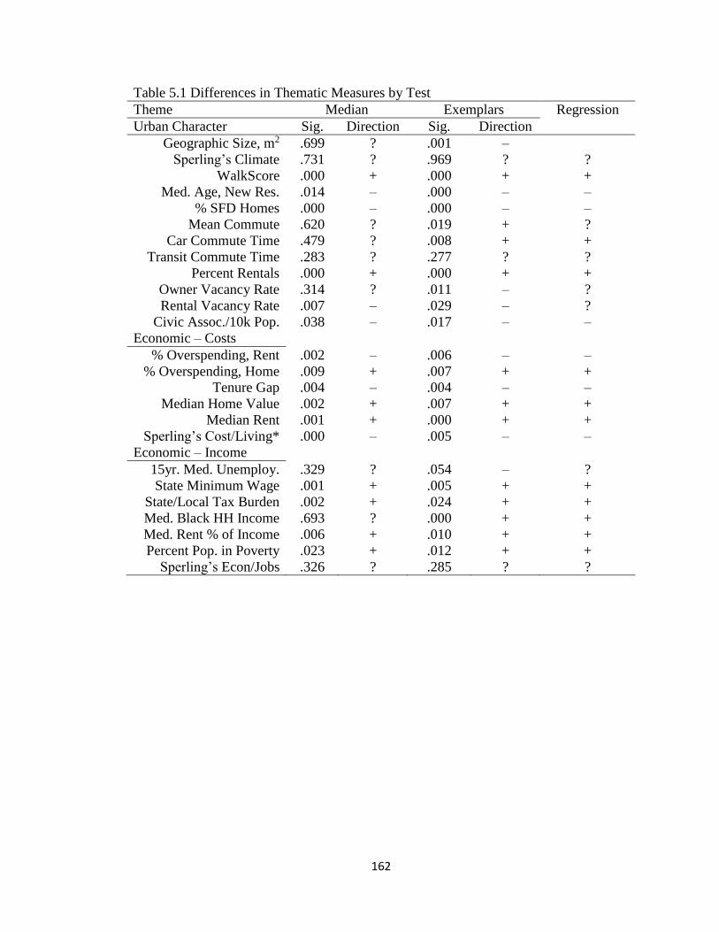


![Introduction to Dependency Grammar [0.2cm] and Dependency ...ufal.mff.cuni.cz/~bejcek/parseme/prague/Nivre1.pdf · Introduction to Dependency Grammar and Dependency Parsing Joakim](https://static.documents.pub/doc/80x56/5b14bded7f8b9a201a8b9282/introduction-to-dependency-grammar-02cm-and-dependency-ufalmffcuniczbejcekparsemeprague.jpg)


