Consumer Demand and the Cost of Living - sfu.capendakur/teaching/econ836/consumer demand...

Consumer Demand and the Cost of Living

Krishna Pendakur

November 1, 2009

Krishna Pendakur () Demand is Awesome November 1, 2009 1 / 26

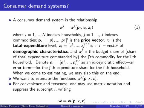
Consumer demand systems?

A consumer demand system is the relationship

w ji = wj (pi , xi , zi ) (1)

where i = 1, ...,N indexes households, j = 1, ..., J indexescommodities; pi = [p1i , ..., p

Ji ]0 is the price vector, xi is the

total-expenditure level, zi = [z1i , ..., zTi ]0 is a T vector of

demographic characteristics, and w ji is the budget share of (shareof total expenditure commanded by) the jth commodity for the ithhousehold. Denote εi = [ε1i , ..., ε

Ji ]0 as an idiosyncratic e¤ect an

error term for the jth expenditure share for the ith household.When we come to estimating, we may slap this on the end.We want to estimate the functions w j (p, x , z).For convenience and terseness, one may use matrix notation andsuppress the subscript i , writing

w = w(p, x , z)Krishna Pendakur (Simon Fraser University) Demand is Awesome November 1, 2009 2 / 26

How are they useful?

Without Integrability

predict the e¤ects of policies that change prices, eg, sales tax changes.

With Integrability

demands w j (p, x , z) can inform us about cost and indirect utilityfunctions.

C (p, f (u, z), z) the cost function giving the minimum cost of utilityf (u); f (V (p, x , z), z) the indirect utility function

The function f is monotonically increasing but unobservable; just thereto emphasise the ordinal nature of the utility function.I will suppress f hereafter.

Krishna Pendakur (Simon Fraser University) Demand is Awesome November 1, 2009 3 / 26

Uses

Macroeconomic policy, vis the ination rate(for average or allhouseholds) (see Crossley and Pendakur 2009).consumer surplus (CV, EV) calculation

C (p1,V (p0, x , z), z) C (p0,V (p0, x , z), z)C (p1,V (p1, x , z), z) C (p0,V (p1, x , z), z)

household (type) specic price indices for poverty, inequality andsocial welfare measurement.

C (p1,V (p0, x , z), z)/C (p0,V (p0, x , z), z)

reveal inter-household comparisons of well-being frombehaviour measure equivalence scales

C (p, u, z1)/C (p, u, z0)

Integrability of estimated consumer demand system allows recovery ofthe cost function (up to f ).


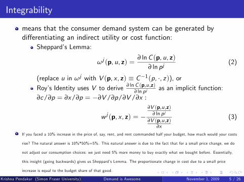
Integrability

means that the consumer demand system can be generated bydi¤erentiating an indirect utility or cost function:

Sheppards Lemma:

ωj (p, u, z) =∂ lnC (p, u, z)

∂ ln pj(2)

(replace u in ωj with V (p, x , z) C1(p, , z)), orRoys Identity uses V to derive ∂ lnC (p,u,z)

∂ ln p j as an implicit function:∂c/∂p = ∂x/∂p = ∂V/∂p/∂V/∂x :

w j (p, x , z) = ∂V (p,u,z)

∂ ln p j

∂V (p,u,z)∂x

(3)

If you faced a 10% increase in the price of, say, rent, and rent commanded half your budget, how much would your costs

rise? The natural answer is 10%*50%=5%. This natural answer is due to the fact that for a small price change, we do

not adjust our consumption choices: we just need 5% more money to buy exactly what we bought before. Essentially,

this insight (going backwards) gives us Sheppards Lemma. The proportionate change in cost due to a small price

increase is equal to the budget share of that good.


More Integrability

Properties of C (V ) imply properties on w j , typically testableproperties.integrability requires homogeneity (cost is HD1 in prices). Thisimplies that absence of money illusion.

homogeneity implies that

w j (λp,λx , z) = w j (p, x , z)

this is equivalent to a condition on the derivatives of demand equations

J

∑k=1

∂w j (p, x , z)∂ ln pk

+∂w j (p, x , z)

∂ ln x= 0. (4)

integrability requires symmetry (cost function is a function). Dene

Γjk (p, x , z) =∂w j (p, x , z)

∂pk+

∂w j (p, x , z)∂x

w k (p, x , z).

Symmetry is satised if and only if

Γjk (p, x , z) = Γkj (p, x , z)Krishna Pendakur (Simon Fraser University) Demand is Awesome November 1, 2009 6 / 26

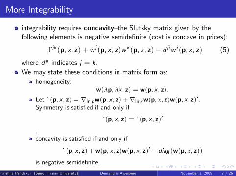
More Integrability

integrability requires concavitythe Slutsky matrix given by thefollowing elements is negative semidenite (cost is concave in prices):

Γjk (p, x , z) + w j (p, x , z)w k (p, x , z) d jjw j (p, x , z) (5)

where d jj indicates j = k.We may state these conditions in matrix form as:

homogeneity:w(λp,λx , z) = w(p, x , z).

Let ` (p, x , z) = rln pw(p, x , z) +rln xw(p, x , z)w(p, x , z)0.Symmetry is satised if and only if

` (p, x , z) = ` (p, x , z)0

.concavity is satised if and only if

` (p, x , z) +w(p, x , z)w(p, x , z)0 diag(w(p, x , z))is negative semidenite.


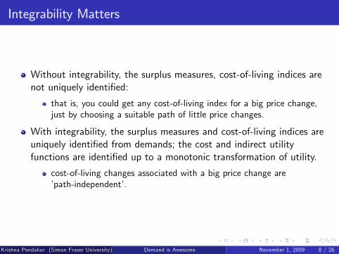
Integrability Matters

Without integrability, the surplus measures, cost-of-living indices arenot uniquely identied:

that is, you could get any cost-of-living index for a big price change,just by choosing a suitable path of little price changes.

With integrability, the surplus measures and cost-of-living indices areuniquely identied from demands; the cost and indirect utilityfunctions are identied up to a monotonic transformation of utility.

cost-of-living changes associated with a big price change arepath-independent.


Parametric estimation

Ignore z for a while.

Can estimate via specifying functional form for demand equations, eg,

w j (p, x) = aj +J

∑k=1

bjk ln pk + bjx ln x ,

where aj , bjk and bjx are parameters estimated by OLS.

Fine for prediction. Not ne for doing surplus or welfaremeasurement.


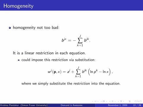
Homogeneity

homogeneity not too bad:

bjx = J

∑k=1

bjk .

It is a linear restriction in each equation.

could impose this restriction via substitution:

w j (p, x) = aj +J

∑k=1

bjkln pk ln x

,

where we simply substitute the restriction into the equation.


Symmetry

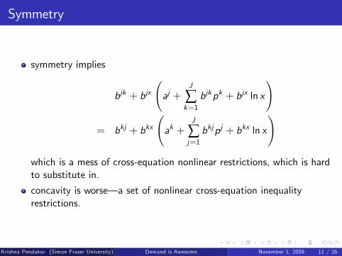
symmetry implies

bjk + bjx aj +

J

∑k=1

bjkpk + bjx ln x

!

= bkj + bkx ak +

J

∑j=1bkjpj + bkx ln x

!

which is a mess of cross-equation nonlinear restrictions, which is hardto substitute in.

concavity is worse a set of nonlinear cross-equation inequalityrestrictions.


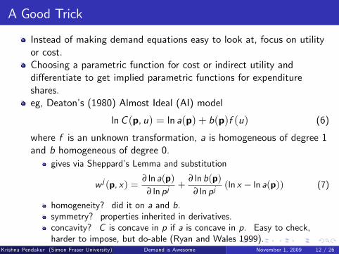
A Good Trick

Instead of making demand equations easy to look at, focus on utilityor cost.Choosing a parametric function for cost or indirect utility anddi¤erentiate to get implied parametric functions for expenditureshares.eg, Deatons (1980) Almost Ideal (AI) model

lnC (p, u) = ln a(p) + b(p)f (u) (6)

where f is an unknown transformation, a is homogeneous of degree 1and b homogeneous of degree 0.

gives via Sheppards Lemma and substitution

w j (p, x) =∂ ln a(p)

∂ ln pj+

∂ ln b(p)∂ ln pj

(ln x ln a(p)) (7)

homogeneity? did it on a and b.symmetry? properties inherited in derivatives.concavity? C is concave in p if a is concave in p. Easy to check,harder to impose, but do-able (Ryan and Wales 1999).


Almost Ideal

Parametric structure

let a be a translog and b is cobb-douglas in prices.

ln a(p) =J

∑k=1

ak ln pk +12

J

∑k=1

J

∑l=1

akl ln pk ln pl

ln b(p) =J

∑k=1

bk ln pk

then get

w j (p, x) = aj +J

∑k=1

ajk ln pk + bj ln x (8)

where

ln x = ln x J

∑k=1

ak ln pk +12

J

∑k=1

J

∑l=1

akl ln pk ln pl .

slightlynonlinear because a stu¤ gets multiplied by b stu¤.


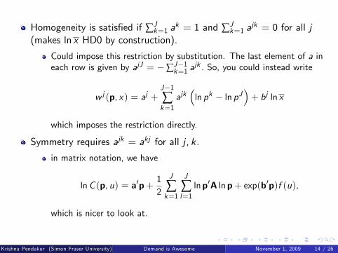
Homogeneity is satised if ∑Jk=1 a

k = 1 and ∑Jk=1 a

jk = 0 for all j(makes ln x HD0 by construction).

Could impose this restriction by substitution. The last element of a ineach row is given by ajJ = ∑J1k=1 a

jk . So, you could instead write

w j (p, x) = aj +J1∑k=1

ajkln pk ln pJ

+ bj ln x

which imposes the restriction directly.

Symmetry requires ajk = akj for all j , k.

in matrix notation, we have

lnC (p, u) = a0p+12

J

∑k=1

J

∑l=1

lnp0A lnp+ exp(b0p)f (u),

which is nicer to look at.


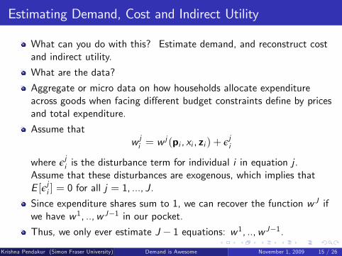
Estimating Demand, Cost and Indirect Utility

What can you do with this? Estimate demand, and reconstruct costand indirect utility.

What are the data?

Aggregate or micro data on how households allocate expenditureacross goods when facing di¤erent budget constraints dene by pricesand total expenditure.

Assume thatw ji = w

j (pi , xi , zi ) + εji

where εji is the disturbance term for individual i in equation j .Assume that these disturbances are exogenous, which implies thatE [εji ] = 0 for all j = 1, ..., J.

Since expenditure shares sum to 1, we can recover the function w J ifwe have w1, ..,w J1 in our pocket.

Thus, we only ever estimate J 1 equations: w1, ..,w J1.Krishna Pendakur (Simon Fraser University) Demand is Awesome November 1, 2009 15 / 26

Estimating the Almost Ideal DS

Given the AI demand system with no demographics, we get

w ji = aj +

M

∑k=1

ajk ln pki + bj ln x i + εji (9)

where

ln x i = ln xi M

∑k=1

ak ln pki 12

M

∑k=1

M

∑l=1

akl ln pki ln pli .

in matrix notation, this is

wi = a+Api + b ln x i + εi ,

ln x i = ln xi a0pi 12

M

∑k=1

M

∑l=1

lnp0iA lnpi ,

which is nicer to look at.Estimate (8) either by nonlinear methods (LS/ML or GMM), oriterative linear methods (Blundell and Robin 1999).


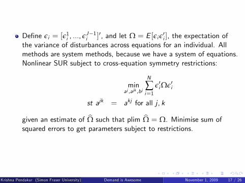
Dene εi = [ε1i , ..., εJ1i ]0, and let Ω = E [εi ε0i ], the expectation of

the variance of disturbances across equations for an individual. Allmethods are system methods, because we have a system of equations.Nonlinear SUR subject to cross-equation symmetry restrictions:

minaj ,ajk ,b j

N

∑i=1

ε0iΩε0i

st ajk = akj for all j , k

given an estimate of bΩ such that plim bΩ = Ω. Minimise sum ofsquared errors to get parameters subject to restrictions.


Hatting it Up

This gives you a bunch of estimates baj ,bajk ,bbj , which imply a log-costfunction

lnC (p, u) = ln a(p) + b(p)f (u)

=M

∑k=1

bakpk + 12

M

∑k=1

M

∑l=1

baklpkpl + M

∏j=1

pkbbk

f (u)

this thing is all hatted up it is full of numbers now.

real expenditure ln xR = lnR(p, x) is the expenditure you need whenfacing some particular price vector p to get the same utility as with xfacing p.Choose p = 1J for convenience.

ln xR = lnR(p, x) = lnC (p, f (u))


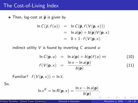
The Cost-of-Living Index

Then, log-cost at p is given by

lnC (p, f (u)) = lnC (p, f (V (p, x)))= ln a(p) + b(p)V (p, x)= 0+ 1 f (V (p, x)

indirect utility V is found by inverting C around u:

lnC (p, u) = ln a(p) + b(p)f (u), (10)

f (V (p, x) =ln x ln a(p)

b(p)(11)

Familiar? f (V (p, x)) = ln x .

So,

ln xR = lnR(p, x) =ln x ln a(p)

b(p).


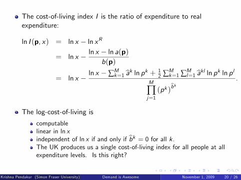
The cost-of-living index I is the ratio of expenditure to realexpenditure:

ln I (p, x) = ln x ln xR

= ln x ln x ln a(p)b(p)

= ln x ln x ∑Mk=1 bak ln pk + 1

2 ∑Mk=1 ∑M

l=1 bakl ln pk ln plM

∏j=1(pk )

bbk .

The log-cost-of-living is

computablelinear in ln xindependent of ln x if and only if bbk = 0 for all k.The UK produces us a single cost-of-living index for all people at allexpenditure levels. Is this right?


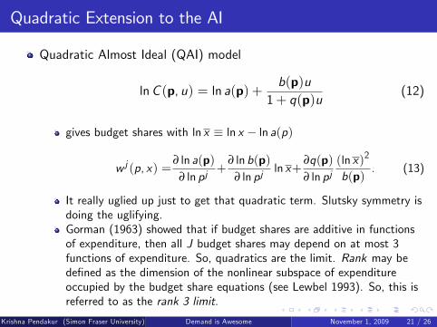
Quadratic Extension to the AI

Quadratic Almost Ideal (QAI) model

lnC (p, u) = ln a(p) +b(p)u

1+ q(p)u(12)

gives budget shares with ln x ln x ln a(p)

w j (p, x) =∂ ln a(p)

∂ ln pj+

∂ ln b(p)∂ ln pj

ln x+∂q(p)∂ ln pj

(ln x)2

b(p). (13)

It really uglied up just to get that quadratic term. Slutsky symmetry isdoing the uglifying.Gorman (1963) showed that if budget shares are additive in functionsof expenditure, then all J budget shares may depend on at most 3functions of expenditure. So, quadratics are the limit. Rank may bedened as the dimension of the nonlinear subspace of expenditureoccupied by the budget share equations (see Lewbel 1993). So, this isreferred to as the rank 3 limit.


Parametric Estimation of Cost-of-Living Indices

Pendakur (2001, 2002) uses the QAI to estimate poverty andinequality with household-specic price indices.

This yields a price index which is di¤erent for rich and poor.

In Canada, use of the QAI price index yields a di¤erent picture ofinequality changing over time

standard indices showing falling inequality over late 1970s; expendituredependent indices show rising inequality.standard indices show slightly rising inequality over 1990s; expendituredependent indices show slightly falling inequality.

Donaldson (1992) showed that the inequality and poverty indicesderived from real expenditurecalculated in this way depends on thechoice of base price vector.

david: There is no substitute for utility.I agree, but that means we have to somehow identify f , whichcardinalises utility.


Nonparametric Estimation of Engel Curves

Rather than specifying a functional form and estimating itsparameters, the idea in nonparametric estimation is to let the dataspeak for themselvesas to the shape of functions.local mean nonparametric estimation uses nearby data to estimatethe height of the regression curve at every point.Pendakur (1999) and Blundell, Duncan and Pendakur (1998) use theshape invariancerestrictions to incorporate demographics intononparametric estimation of Engel curves (w j (x)) and to estimateequivalence scales.

local mean estimator is

w j (x) =∑Ni=1 Kh(xi x)w

ji

∑Ni=1 Kh(xi x).

Kh is kernel function, eg, Kh(u) = ϕ( uh ) where ϕ is the standardnormal density function.At each x , w j (x) is the WLS estimate with w j on the LHS and aconstant on the RHS with weights Kh(xi x).


Blundell, Duncan and Pendakur show that partially additive e¤ectsare NOT integrable.

get nonparametric estimates of Engel curves for each demographictype. Find the closest shape-invariance satisfying engel curves for alldemographic types.

maintaining the assumption of ESE implies shape-invariance, which issu¢ cient to identify equivalence scales even without imposingparametric structure on Engel curves.

Pendakur (2004) uses similar restrictions to estimate lifetimeequivalence scales without imposing parametric structure.


Nonparametric Estimation of Consumer Demand Systems

an Engel curve is not a demand system. We need shares over p, x , z,and we need to impose integrability to get prices indices.

Haag, Hoderlein and Pendakur (2009) develops a methodology fornonparametric estimation of integrable consumer demand systemsand price indices.

The trick is to use local polynomial estimation.

Here, at each point in the domain, w j (p, x , z) is the WLS estimate ofa model with W j on the LHS and a polynomial in p, x , z on the RHSwith weights given by the Kh.

Recall that integrability is a set of conditions on derivatives. Theseare hard to impose on local mean estimators, but easy to impose onlocal polynomials.

The r 0th derivative of a local polynomial is just the coe¢ cient on ther 0th term.


Where should we go?

Measurement error (eg, Chesher et al, Review of Economic Studies,2002) remains a big problem.Preference Heterogeneity (Lewbel and Pendakur 2009)non- and semi-parametric exibility (Lewbel and Pendakur 2009;Haag, Hoderlein and Pendakur 2009; Pendakur and Sperlich 2009).Lack of price variation means price e¤ects are largely gotten fromtheir indirect rather than direct e¤ects in QAI, price e¤ects comefrom intercepts and not from price derivatives.Cardinalise utility. Money metrics are not a good substitute for utility(Donaldson 1992; Roberts 1980), but we need to know the shape ofutility over expenditure.Are nonparametrics really worth the trouble? I suspect that the bestuse of all this nonparametric demand stu¤ is as a diagnostic ofparametric models.

Nonparametric estimators are local estimators only.Nonparametric estimators require more data than we typically have.


Date post:	16-Mar-2019
Category:	Documents
Upload:	trinhtruc
View:	215 times
Download:	0 times

Consumer Demand and the Cost of Living - sfu.capendakur/teaching/econ836/consumer demand...

Documents