The Rodney L. White Center for Financial Research

Consumer Sentiment: Its Rationality and Usefulness in Forecasting Expenditure – Evidence from the Michigan Micro Data

Nicholas S. Souleles

03-02

The Rodney L. White Center for Financial Research The Wharton School

University of Pennsylvania 3254 Steinberg Hall-Dietrich Hall

3620 Locust Walk Philadelphia, PA 19104-6367

(215) 898-7616

(215) 573-8084 Fax http://finance.wharton.upenn.edu/~rlwctr

The Rodney L. White Center for Financial Research is one of the oldest financial research centers in the country. It was founded in 1969 through a grant from Oppenheimer & Company in honor of its late partner, Rodney L. White. The Center receives support from its endowment and from annual contributions from its Members. The Center sponsors a wide range of financial research. It publishes a working paper series and a reprint series. It holds an annual seminar, which for the last several years has focused on household financial decision making. The Members of the Center gain the opportunity to participate in innovative research to break new ground in the field of finance. Through their membership, they also gain access to the Wharton School’s faculty and enjoy other special benefits.

Members of the Center 2001 – 2002

Directing Members

Ford Motor Company Fund Geewax, Terker & Company

Morgan Stanley The Nasdaq Stock Market, Inc.

The New York Stock Exchange, Inc.

Members

Aronson + Partners Bear, Stearns & Co., Inc. Exxon Mobil Corporation

Goldman, Sachs & Co. Spear, Leeds & Kellogg

Founding Members

Ford Motor Company Fund

Merrill Lynch, Pierce, Fenner & Smith, Inc. Oppenheimer & Company

Philadelphia National Bank Salomon Brothers

Weiss, Peck and Greer

Consumer Sentiment: Its Rationality and Usefulness in Forecasting Expenditure

– Evidence from the Michigan Micro Data

Nicholas S. Souleles

Finance Department University of Pennsylvania

and NBER

this draft: July 2001 ___________________________ For helpful comments I thank Martin Browning, Chris Carroll, Roger Ferguson, Todd Sinai, Sarah Tanner, and seminar participants at Chicago, Princeton, Tilburg, the Federal Reserve Board of Governors, McMaster, York, the NBER summer workshop and the Wharton macro lunch. I am very grateful to Richard Curtin for providing data and feedback, and to Hoon Ping Teo for excellent research assistance. Of course, none of these people is responsible for any errors herein.

Consumer Sentiment: Its Rationality and Usefulness in Forecasting Expenditure

– Evidence from the Michigan Micro Data

this draft: July 2001

Abstract: This paper provides one of the first comprehensive analyses of the household data

underlying the Michigan Index of Consumer Sentiment. This data is used to test the rationality of consumer expectations and to assess their usefulness in forecasting expenditure. The results can also be interpreted as characterizing the shocks that have hit different types of households over time. Expectations are found to be biased, at least ex post, in that forecast errors did not average out even over a sample period lasting almost 20 years. People underestimated the disinflation of the early 1980's and in the 1990's, and generally appear to underestimate the severity of business cycles. Forecasts are also inefficient, in that people’s forecast errors are correlated with their demographic characteristics and/or aggregate shocks did not hit all people uniformly.

Further, sentiment is found to be useful in forecasting future consumption, even controlling for lagged consumption and macro variables like stock prices. This excess sensitivity is counter to the permanent income hypothesis [PIH]. Higher confidence is correlated with less saving, consistent with precautionary motives and increases in expected future resources. Some of the rejection of the PIH is found to be due to the systematic demographic components in forecast errors. But even after controlling for these components, some excess sensitivity persists. More broadly, these results suggest that empirical implementations of forward-looking models need to better account for systematic heterogeneity in forecast errors.

JEL classification: E21 [Macroeconomics: Consumption; Saving]

Keywords: Consumer sentiment (confidence); Permanent income hypothesis; Excess sensitivity; Rational expectations, Forecast errors, Shocks; Unobserved heterogeneity.

1

Debate over the usefulness of consumer sentiment surveys in forecasting economic

activity began soon after their introduction in the 1940’s. The possibility that a decline in

consumer confidence helped cause or worsen the 1990-91 recession renewed interest in the

debate. Most recent studies of sentiment have focused on the time series relationship between

aggregate consumption and the two main aggregate indices of sentiment, the Michigan Index of

Consumer Sentiment [ICS] and the Conference Board Consumer Confidence Index. This paper,

by contrast, provides perhaps the first comprehensive analysis of the household-level data that

underlies the ICS, the Michigan Survey of Consumer Attitudes and Behavior [CAB]. The

attention that the ICS receives, from policymakers, academics, and the business community,

itself warrants an analysis of the underlying data. There are also a number of methodological

advantages to such an analysis.

First, with micro data one can assess the rationality of household expectations. Most

previous rationality tests have limited their focus to inflation expectations, just one of the many

variables that will be examined here. Also, the tests have generally used aggregated data, or at

most short micro panels. But when agents’ information sets differ, aggregation can lead to

spurious rejections of rationality. The average of rational individual forecasts need not be a

rational forecast conditional on any single information set (Keane and Runkle [1990]). And even

if individual forecasts are perfectly rational, it might take a long time -- perhaps multiple

business cycles -- for forecast errors to average out. Hence to test rationality it is important to

use micro data on expectations over long sample periods. Unfortunately such data is not usually

available. The CAB survey, however, is unique in containing almost 20 years of monthly

household expectations data. This paper exploits its panel aspect to test more cleanly than usual

whether expectations are unbiased and efficient. The results can also be interpreted as explicitly

2

characterizing the shocks that have hit different types of households over time, across business

cycles and policy regimes. In addition to its welfare implications, such a characterization is of

methodological interest, because both theoretical and empirical models are generally sensitive to

the assumptions made about shock processes. In particular, many models assume that

"aggregate" shocks affect all households uniformly.

Second, this paper assesses whether the sentiment surveys are useful in predicting

behavior, specifically household spending. The canonical permanent income (or life-cycle)

hypothesis [PIH] provides a natural setting for this assessment. One of the central implications of

the PIH is that current consumption should incorporate all the information available to an agent.

However the econometrician does not independently observe the contents of agents' information

sets, so tests of this implication usually need to make strong assumptions, inferring agents’

expectations econometrically. This paper instead uses the direct survey data on expectations in

the CAB data. This data is matched, using a rich set of demographic variables, with the

Consumer Expenditure Survey [CEX], which has the most comprehensive micro data on

expenditure. The resulting test is whether the expectations data contain additional information,

beyond that in current consumption, that helps predict future consumption. Previous studies of

the excess sensitivity of consumption to sentiment have used aggregate sentiment data, but

aggregation can induce spurious excess sensitivity even when there is none at the micro level

(Attanasio and Weber [1995]). The construction of the ICS is not consistent with the

construction of aggregate consumption. For instance the ICS is an equal-weighted average of the

sentiment of the CAB survey respondents, which ignores differences in the scale of consumption

across respondents.

With micro data one can also more readily investigate the sources of any excess

3

sensitivity. One alternative hypothesis that has not previously received much scrutiny is that

forecast errors might not be classical, but rather contain systematic components correlated with

the excess sensitivity regressor. For instance, over the sample period high income households

might on average have been optimistic about the future, and might have happened to receive

disproportionately positive shocks. In this case increases in their consumption, and so a positive

correlation between consumption and sentiment, would not be inconsistent with the PIH. More

broadly, Chamberlain [1984] and others have pointed out that systematic forecast errors can be a

potential problem in estimating any rational expectations (or forward-looking) model in a short

panel. Because direct measures of households’ forecast errors are available here, it is possible to

test this point directly.

Third, the aggregate ICS ignores potentially useful information available in the micro

CAB data. As already noted, the ICS neglects the cross-sectional distribution of sentiment. This

distribution might be useful in predicting the expenditure of different groups of consumers, or

even aggregate expenditure insofar as the relation between expenditure and sentiment at the

household level does not aggregate up. In the ICS a given respondent's sentiment is in turn the

sum of her answers to five very different survey questions, which makes it hard to interpret.

This paper examines, separately for each question, whether the survey responses help forecast

household spending. This examination also addresses one perennial question in the time-series

literature: Does sentiment provide information useful in forecasting, above and beyond the

information contained by other available macro variables like stock prices? By controlling for

time effects in the micro data, one can exploit purely cross-sectional variation that is perforce

orthogonal to any macro variable.

To preview the results, expectations appear to be biased, at least ex post, in that forecast

4

errors did not average out even over a sample period lasting almost 20 years. This bias is not

constant over time; it is related to the inflation regime and the business cycle. People

underestimated the disinflation of the early 1980's and in the 1990's, and generally appear to

underestimate the severity of business cycles. Forecasts are also inefficient, in that people’s

forecast errors are correlated with their demographic characteristics and/or aggregate shocks did

not hit all people uniformly. For instance, during recent expansions high income households

received relatively good shocks, but low income households continued to receive somewhat

negative shocks, consistent with ongoing, unexpected skill-biased technical change. Further,

sentiment is useful in forecasting future consumption, even beyond lagged consumption and

other macro variables, counter to the PIH. Higher confidence is correlated with less saving,

consistent with precautionary motives and increases in expected future resources. Some of the

rejection of the PIH is found to be due to the systematic demographic components in forecast

errors. But even after controlling for these components, some excess sensitivity persists. More

broadly, because forecast errors are correlated with household demographic characteristics, they

will be correlated with many regressors of interest in forward-looking models. This suggests that

systematic heterogeneity in forecast errors is in practice a general and potentially serious

problem.

The paper begins by surveying related studies in Section I. Section II describes the data

and Section III, the econometrics. Section IV tests the rationality of expectations and more

generally characterizes the properties of forecast errors. Section V tests whether sentiment helps

forecast expenditure, and if so whether this is due to systematic demographic components in

forecast errors. Section VI concludes.

5

I. Related Studies

Most tests of the rationality of surveyed expectations have focused on inflation

expectations of economists (e.g., Keane and Runkle [1990]). A few studies have examined the

inflation expectations of consumers in general, using the aggregated Michigan data (Maddala,

Fishe, and Lahiri [1981], Gramlich [1983], Batchelor [1986]). These studies mostly analyzed the

Michigan question that allows only qualitative responses about the future path of inflation

(up/down/no change). To use this question quantitatively the studies typically made strong

assumptions to derive a continuous-valued expectations time-series from the aggregated data.

Moreover, as already noted, because of aggregation bias the implications of these tests for

individual rationality are not straightforward. One study, Batchelor and Jonung [1989], examined

micro-level data on the inflation expectations of a small and short (one-year) Swedish panel,

finding evidence of bias and inefficiency. However, rationality does not require that people’s

expectations be on target over the course of only a single year.

Flavin [1991], Dominitz [1993], and Alessie and Lusardi [1997] used micro-level data on

income expectations to predict future income. While they did not formally test the rationality of

these expectations, they did find a positive, if not very large, correlation between them and future

realizations of income. Das and van Soest [1999] tested the rationality of income expectations in

a Dutch dataset. They found that income expectations were on average too low relative to

subsequent realizations. However, their data is also limited to a relatively short panel (1984-88).

As shown below, even five years might be too small to allow forecast errors to average out.

Expectations might have been rational ex ante, but might not appear rational ex post. For

instance the sample might by chance have received unexpectedly good income realizations over

the period. This paper, by contrast, uses almost twenty years of micro-data, for many different

6

kinds of expectations questions. Of course, even twenty years might not be a long enough

period. But such a result would be as significant as a finding of irrationality, because most micro

studies are limited to datasets with a shorter sample period.

Even if expectations are not fully classical, people might still act on them and so they

might help forecast spending. Of particular interest is whether sentiment surveys contain

predictive information not available in other variables, most saliently current consumption. Two

important recent studies have examined this issue using aggregate time series data, in an Euler-

equation framework.1 Carroll, Fuhrer, and Wilcox [1994] used the ICS and Acemoglu and Scott

[1994] used a related Gallup poll in Britain. Both found significant excess sensitivity of

consumption to sentiment, and suggested that sentiment might be picking up precautionary

motives. But under this interpretation the sign of their estimated excess sensitivity is somewhat

surprising: increased confidence led to a steeper consumption profile, i.e. to increased saving;

whereas the simplest precautionary story would have increased confidence lead to less saving.2,3

Also, it remains an open question whether other variables might already incorporate the

information in aggregate sentiment. While Carroll, Fuhrer, and Wilcox show that the ICS

contains additional information beyond that available in aggregate income, other studies have

found that financial variables, in particular stock prices, significantly reduce the contribution of

aggregate sentiment in forecasting (Friend and Adams [1964], Ludvigson [1996]). By revisiting

1 The earliest study of which I am aware that used an Euler-equation framework to analyze sentiment is an unpublished Federal Reserve Board working paper by Burch and Gordon [1985], again using aggregate data. The Gulf War triggered a number of additional studies of aggregate sentiment, often by researchers in the Federal Reserve System (e.g., Throop [1992] and Carroll, Fuhrer, and Wilcox). 2 A steeper consumption profile implies increased saving under the null hypothesis of the PIH. Outside the PIH this implication need not hold. 3 Carroll, Fuhrer, and Wilcox note that frictions in consumption, e.g. due to habits, can explain the sign of their results. Acemoglu and Scott suggest a different explanation: higher confidence might be correlated with higher levels of income, which in turn might be correlated with a higher variance in income, and so a greater precautionary motive.

7

the matter using micro data, this paper avoids potential aggregation bias and takes advantage of

additional information in the cross-sectional distribution of sentiment.

Only a few papers have used micro-level expectations data in an Euler-equation

framework.4 Two of the most interesting are by Flavin [1991] and Alessie and Lusardi [1997],

who used income expectations as instruments for income in the related Euler equation for saving.

Both rejected the PIH. However, both studies were limited to essentially single cross-sections

(the 1967 SCF and a 1986 Dutch panel, respectively), leaving systematic heterogeneity in

forecast errors a potential problem.5 To illustrate, Mariger and Shaw [1993] showed that in the

Panel Study of Income Dynamics the excess sensitivity coefficient on lagged income growth

varies in sign from year to year. For instance, the three-year sample used by Hall and Mishkin

[1982] happens to yield a negative coefficient, but other short samples yield a positive

coefficient. Mariger and Shaw conjectured that this instability might be due to aggregate shocks.

But in contrast to this paper, without an independent measure of these shocks they were unable

to test their conjecture directly.

II. Data

A. The Survey of Consumer Attitudes and Behavior [CAB]

The CAB is a nationally representative survey that since 1978 has been collected

4 Some of the earliest studies of sentiment, in the 1950’s and 1960’s, also used micro data. Their results were mixed. (See McNeil [1974] for a summary.) They generally had small sample sizes and short time horizons. Further, it is often hard to interpret their results because the models of consumption they used are generally different from current models. Outside the consumption literature, Nicholson and Souleles [2001, 2001a] find that income expectations of medical students help predict their specialty choice and subsequent practice behavior. They also trace the source of physicians’ forecast errors to particular changes in their practices and health-care market, such as the emergence of HMOs. 5 A recent paper by Jappelli and Pistaferri [1998] uses income expectations from an Italian Survey in an Euler equation. While they do not find excess sensitivity, they note this might be due to measurement error, especially in the timing of their expectational questions vis-à-vis the other variables. Their data contains two cross-sections of expectations.

8

monthly. This paper uses the data from December 1978 through June 1996. In recent years

about 500 households are sampled each month, in the earlier years two to three times as many

were sampled. The five questions that comprise the widely followed ICS are as follows. The

allowed responses are in brackets (underlining in original).

QFPr. (Financial Position realization) We are interested in how people are getting along financially these days. Would you say that you (and your family living there) are better off or worse off financially than you were a year ago? [better now, same, worse now]

QFPe. (Financial Position expectation) Now looking ahead—do you think that a year from

now you (and your family living there) will be better off financially or worse off, or just about the same as now? [will be better off, same, will be worse off]

QBC. (Business conditions) Now turning to business conditions in the country as a whole—do

you think that during the next twelve months we’ll have good times financially, or bad times, or what? [good times, good times with qualifications, pro-con, bad with qualifications, bad times]

QBC5. (Business conditions, 5 year horizon) Looking ahead, which would you say is more

likely—that in the country as a whole we’ll have continuous good times during the next 5 years or so, or that we will have periods of widespread unemployment or depression, or what? [good times, good times qualified, pro-con, bad times qualified, bad times]

QDurs. (Durables purchases) About the big things people buy for their homes—such as

furniture & refrigerator, stove, television, and things like that. Generally speaking, do you think now is a good or bad time for people to buy major household items? [good, pro-con, bad]

Some economists are wary of subjective survey questions such as these. Instead of

offering an exegesis, this paper will formally test the rationality of the responses and see whether

they are correlated with behavior, specifically whether they help forecast spending.6,7 In a related

paper, Souleles [2001] shows that these same questions help predict household purchases of

6 As for the particular wording of the questions, they have the virtue of having stayed the same over the sample period. Also, it is worth noting that most household-level data, not just sentiment, is based on households’ self-reports. 7 Carroll, Fuhrer, and Wilcox [1994] and others have shown that the aggregate ICS helps forecast aggregate consumption. Studies of the CAB inflation expectations, described below, have found that they are helpful in

9

risky securities. Even controlling for past stock returns, households that are pessimistic about the

future buy fewer risky securities, ceteris paribus.8

A few additional notes are in order. First, questions QBC, QBC5, and QDurs ask the

respondent about aggregate economic activity, while QFPr and QFPe ask about the household’s

own financial position. This suggests there might be more cross-sectional variation in QFPr and

QFPe than in the other variables. Second, QFPe, QBC, and QBC5 ask about the future9, whereas

QFPr asks about the past year and QDurs asks about the present. Third, the wording of QFPe

("e" for expectation) matches that of QFPr ("r" for realization). Thus if someone is asked QFPe

this year, and then QFPr next year, QFPe provides a forecast of what his answer to QFPr will be.

However the response to QFPe is constrained to one of three categories (better, worse, or the

same). Therefore the analysis will accommodate the discrete, ordered nature of this and the other

variables. For convenience, the better states (“better” or “good” or “good with qualification”)

are usually coded as +1, the intermediate states (“same” or “pro-con”) as 0, and the worse states

(“worse” or “bad” or “bad with qualification”) as -1.10

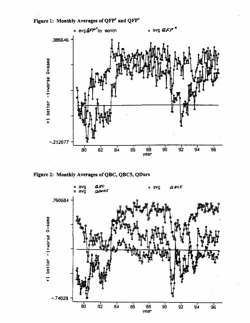
Figures 1 and 2 show the average response for each question month-by-month. All five

variables are procyclical. Notably, the forward-looking QFPe appears to lead the backward-

looking QFPr. For instance QFPe recovers more quickly from both the 1980-81 recession and

the 1990 invasion of Kuwait. Nonetheless the two aggregate time series are highly correlated, at

predicting CPI inflation, sometimes even better predictors than the inflation forecasts from professionals (Thomas [1999]). 8 A one-standard-deviation decline in QFPe leads to about a 50% increase in the number of households selling securities and a 30% decrease in the number buying securities, albeit starting from small numbers of households buying and selling. These magnitudes are larger than the effects of a one-standard-deviation decline in past stock returns. For another application of the CAB, to tax cuts, see Shapiro and Slemrod [1995]. 9 These three questions make up the Expectations sub-index of the ICS, which in turn is a component of the Index of Leading Economic Indicators.

10

about 0.8.

The CAB survey asks many additional questions. This paper will focus on the five

questions above because they comprise the ICS, but will also consider the most salient of the

additional questions, listed in the Appendix. There are two matching questions on business

conditions related to QBC. Since one can be taken as the expectation of the other, they will be

denoted QBCe and QBCr. There are also matched questions about changes in prices, QPe and

QPr, and changes in the household’s real income, QYe and QYr, over the following year and

previous year respectively. QUe asks whether the respondent expects the national unemployment

rate to increase or decrease over the next year. Even though there is no matching realization

question about perceived unemployment over the past year, this question is used because

precautionary saving might be sensitive to unemployment expectations.11 The answers to all

these questions are again discrete and ordered. For business conditions QBC and household

income QY, again +1 denotes the good state. But note that for inflation QP and unemployment

QU, +1 denotes the bad state (an increase in inflation or unemployment). There are also

matched pairs of continuous, quantitative questions, which can be used to verify that the

discreteness of the previous questions is not driving their results. The continuous questions

concern the inflation rate over the next and past 12 months (denoted by QΠe and QΠr) and the

growth rate of the household's income (QGYe and QGYr). Unlike the five ICS questions (QFPr

to QDurs), these additional questions were not always asked in every month of the sample

period.

10 The ICS uses this coding in a diffusion index. For each question, the aggregate value at a given time is the number of people answering +1 at that time minus the number of people answering -1. Such indexes omit the people answering 0, as well as the distribution of the rest of the answers across people of different characteristics. 11 Carroll [1992] was amongst the first to explicitly link QU to precautionary motives, in an aggregate time-series context. More recently Carroll et. al. [1996] examine the effects of cross-sectional differences in (ex post)

11

Even though the CAB surveys are archived as independent cross-sections, there is a short

panel aspect to them that has not previously been much exploited: Households are reinterviewed

once and re-asked the same sentiment questions. Much effort was expended by the author to

create a single, consistent panel dataset from the entire history of CAB cross-sections. Explicit

forecast errors could then be calculated for the matched pairs of questions by taking a realization

from the second interview (e.g., QYr2) and subtracting the corresponding expectation from the

first interview (QYe1). Thus, for a given household the error regarding income is defined as εY

≡ QYr2 - QYe

1. Errors for financial position, business conditions, and prices are defined

similarly: εFP ≡ QFPr2 - QFPe

1, εBC ≡ QBCr2 - QBCe

1, and εP ≡ QPr2 - QPe

1, respectively.

Given the coding of the underlying variables Q in {-1,0,1}, these errors ε take on values in the

set {-2, -1, 0, 1, 2}. With a few exceptions, since December 1978 the second household

interview in the CAB survey has taken place six months after the first interview. For

consistency, for calculating forecast errors the sample is started in December 1978 and is limited

to households reinterviewed after six months. Since the forecast horizon written into most of the

expectational questions is one year, not six months, the timing in forming the errors ε is

unavoidably inexact. Nevertheless the timing is exogenous and unsystematic, since the sample

covers every month over almost two decades.12 Extensions below will verify that this timing

issue does not drive the results.

For the quantitative questions on expected inflation and income growth, QΠe and QGYe,

unemployment rates on balance sheets in the Survey of Consumer Finances. The results are consistent with precautionary saving. 12 Suppose a household's first interview is in month t, and Qe

1 refers to the expected change in some variable X between months t and t+12, and Qr

2 from the second interview elicits the realized change Xt+6-Xt-6. Then the timing mismatch corresponds to the term [(Xt-Xt-6)-(Xt+12-Xt+6)]. This term can reasonably be assumed to average out over the long sample period, and in the cross-section. E.g., events that take place in months 7 to 12 after the first interview for one household, will appear in months 1 to 6 before the first interview for other households interviewed later, and hence tend to average out.

12

continuous forecast errors can be computed analogously, e.g. εGY ≡ QGYr2 - QGYe

1.13 For

inflation there is more flexibility in computing the errors since the actual consumer inflation rate

can be measured independently via the CPI. Therefore three different forecast errors εΠ are

computed. The “subjective” error εΠsubj ≡ QΠr2 - QΠe

1 compares the inflation rate the

respondent expects over the next 12 months, taken from the first interview, with the inflation rate

the respondent believes was realized over the past 12 months, taken from the second interview

six months later. Again, because the realization variable is not elicited twelve months later the

timing is not exact. To avoid this problem, the “objective” error εΠobj ≡ Πr12 - QΠe

1 compares

the 12-month inflation rate the respondent expected in the first interview with the actual inflation

rate over the next 12 months, according to the CPI (Πr12). In this case the timing is exact. The

third error εΠ6obj ≡ Πr

6 - QΠe1 uses for its realization the CPI inflation rate over only the first six

months following the first interview, annualized. This error can be contrasted with εΠobj to

investigate the effects of the six-month mistiming in the other forecast errors.

The CAB survey also includes a number of demographic questions. Since some of these

changed across surveys, great care was taken to create a set of demographic variables consistent

across the entire sample (and consistent with the CEX). The Appendix provides more details.

The main sample exclusion concerns the survey respondent. The sample drops an observation

when there is a married couple in the household but the respondent is neither the husband nor

spouse. (Most such respondents appear to be older children of the couple.) This should help

13 There is an additional complication regarding the timing of QGYe. The corresponding realization question elicits the level of household income (not the growth rate) in the previous calendar year. Since the second interview follows after only six months, to compute a non-zero growth rate for income from one year to the next, QGYr, the sample for this question must be limited to households whose first interview takes place in the second half of the year, so that the second interview takes place in the following calendar year. By contrast, the expectational question QGYe

1 asked in the first interview refers to income growth over the next twelve months, so its reference period will somewhat lag the reference period of the computed QGYr.

13

make the respondent’s answers more representative of the entire household. Demographic

variables referring to the reference person were switched to refer to the head of household (i.e.,

for a married couple, the male, following the convention in the literature). An additional

exclusion was adopted in forming the subjective forecast errors (i.e., all but the objective

inflation errors): to make the answers in both interviews more comparable, the same person had

to be the respondent in both interviews.

B. The Consumer Expenditure Survey [CEX]

Because the CAB survey does not include much data on expenditures, it is matched with

the Consumer Expenditure Surveys, from 1982-1993.14 CEX households are interviewed four

times, three months apart (though starting in different months for different households). The

reference periods for expenditure cover the three months before each interview. Strictly speaking

the Euler equation used below applies only to nondurable consumption, but for gauging the

aggregate effect of sentiment total consumption also matters. Indeed, some analysts have

suggested that sentiment matters most for durables purchases. Therefore, for each household-

quarter, both real nondurable expenditure and real total expenditure were computed (1982-84 $).

The CEX sample was selected in standard ways to improve the measurement of

consumption. A household was dropped from the sample if there were multiple “consumer

units” in the household, or the household lived in student housing or the head of household was a

farmer. A household-quarter was dropped if no food-expenditure was recorded in the quarter, or

any food was received as pay in the quarter. The Appendix provides further details about the

data.

14

III. Econometric Specifications

The sentiment of the CEX households will be imputed from the sentiment of

demographically similar households in the CAB data survey. Since the surveys contain a rich,

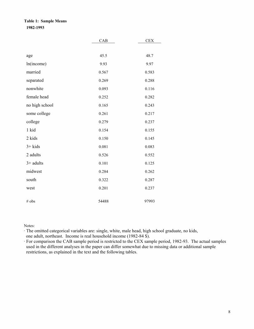
overlapping set of demographic variables, the imputation can be made very fine. Table 1 shows

the means of the main variables used. The CAB sample is somewhat more highly educated and

likely to live in the South. But generally the means are rather similar, as one would expect from

two representative datasets. The imputation proceeds in two steps.

The first step takes place in the CAB data. For the discrete sentiment variables, since

their responses are ordered, both linear and ordered probit models will be estimated. In the

latter, for a given sentiment variable Q ∈ {-1, 0, +1} and household i, let Qi,t* be the

corresponding (continuous) latent index at time t, representing i's underlying sentiment or

confidence. Qi,t* is assumed to take the following form:

Qi,t* = a0′timet + a1′Zit + ui,t. (1)

Except for the questions on inflation and unemployment, larger values of Q* reflect better states.

Z is the vector of demographic instruments used to link the two datasets, from Table 1. time

includes a full set of month dummies (a different dummy for each month of each year). These

dummies will allow for changes in the average level of sentiment from month to month. Since

the cross-sectional distribution of sentiment around the average can also change over time, some

of the demographic variables are interacted with the month dummies. Because there are well

over 100 months in the sample, to keep the computational requirements tolerable only a few

variables could be interacted simultaneously. Preliminary analysis found that for most sentiment

questions the effects of age and income varied the most significantly over time, so Z also

14 The first wave of the CEX, 1980-81, is not used because its data are generally poorer than the data from the

15

includes month-interactions for these two variables. Ordered logits were also estimated, but

since the results were quite similar they are not reported. For the continuous variables QGY and

QΠ, the same functional form in (1) is estimated by OLS.

The second step takes place in the CEX. The estimated coefficients from the first step, â0

and â1, are used to impute the (continuous index value) level of sentiment $Q of the CEX

households with the same demographic characteristics Z:

$Q i,t = â0′timet + â1′Zit . (2)

Lagged $Q is then added to a standard linearized Euler equation for consumption. For household

i the change in log consumption between periods t+1 and t is specified as

dlnCi,t+1 = b0′timet + b1′Wi,t+1 + b2 $Q i,t + ηi,t+1. (3)

Following Zeldes [1989], Dynan [1993], Lusardi [1996], and Souleles [1999], W will include the

age of the household head and changes in the number of adults and in the number of children.

These variables help control for the most basic changes in household preferences over time.15

For a given household the consumption changes in equation (3) are taken over successive

three-month periods. To keep the sentiment data timely, the time-varying components of $Q i,t are

estimated from the CAB survey corresponding to the first of the three months covered by Ci,t.

For instance, consider the case in which Ci,t records consumption in November 1990 to January

1991 (and Ci,t+1 covers February-April 1991). In equations (1) and (2), the month dummies timet

and the month-interacted variables in Zit would then correspond to the November 1990 CAB

following waves. 15As Deaton [1992] notes, by restricting the variables in Z or expanding the variables in W, it would be possible to eliminate most any excess sensitivity. Therefore W is restricted to this commonly used set of controls (age and changes in family size), for comparison with previous studies and to retain power to test for excess sensitivity and for systematic heterogeneity in forecast errors. See the survey of specifications in Table 5.1 of Browning and Lusardi [1996].

16

survey. $Q i,t is therefore predetermined in equation (3), and so under the PIH the coefficient b2

should be zero. That is, given current consumption, current sentiment should not help predict

future consumption.

OLS estimation of equation (3) would neglect the fact that $Q is a generated regressor.

To take this into account the two-sample instrumental-variables technique of Angrist and

Krueger [1992] will be used, although here the technique is not required for consistency but only

to adjust the standard errors for the additional variation arising from the first estimation step.

This technique requires that both estimation steps be linear, so for the reported excess sensitivity

tests equation (1) is estimated by OLS even for the discrete sentiment questions. A previous

version of this paper reported instead the ordered probit results for the discrete questions.

Comparing the results shows that the discreteness of Q makes very little difference to the excess

sensitivity tests; the signs and significance of the coefficients in equation (3) are quite similar.16

The standard errors in (3) are also corrected for general heteroscedasticity and serial correlation

by household.

The month dummies in equation (3) control for all aggregate (uniform) effects, including

seasonality, aggregate interest rates, and any other macro variables like stock prices that might

incorporate some of the same information available in the aggregate time series of sentiment.

Since the same time dummies are used in the first step in equation (1), in (3) they effectively

partial out the monthly average level of sentiment, leaving only cross-sectional variation in $Q .

16 Jappelli, Pischke, and Souleles [1999] also applied this two-sample estimator to excess sensitivity tests. They too imposed linearity on a first-step specification that was originally discrete, and found that the final excess sensitivity results were not sensitive to this imposition. Alternatively, equations (1) and (3) can be jointly bootstrapped, estimating equation (1) by ordered probit. However each ordered probit takes many hours, making bootstrapping infeasible for the full set of results below. The bootstrap standard errors were however computed for the first specification in Table 3 (for QFPr for nondurable consumption). The resulting significance levels for the coefficients in equation (3) were similar to those reported using the two-sample estimator.

17

Although using these time dummies makes it harder to find a significant effect of sentiment in

predicting consumption, they provide a crisp test of whether the micro data contains useful

information not available in the aggregated data.

This paper also tests the rationality of people’s forecasts, namely their unbiasedness and

efficiency. The results can also be interpreted as characterizing the shocks that have ex post hit

different types of households. Efficiency requires that forecast errors be uncorrelated with any

variable in an agent’s information set at the time of forecast; otherwise the forecast does not take

advantage of all available information. Time-series analyses of the efficiency of inflation

expectations often test for serial correlation in inflation forecast errors. However, for each

sentiment question the CAB data contains only one forecast error per household, so it is

impossible to test for serial correlation at the micro level.17 This paper instead tests efficiency by

looking for systematic demographic components in households’ forecast errors. The focus is on

cross-sectional heterogeneity, because that is the variation available in the CAB data, and the

variation exploited in most excess sensitivity tests in micro data.

Specifically, heterogeneity in forecast errors will be analyzed using a specification

similar to equation (1), but with the errors ε (defined above) as the dependent variable:

εi,t+1* = d0′timet + d1′Zit + vi,t+1, (4)

where t refers to the first household interview in the CAB data, t+1 to the second interview. For

instance, for income the error is εYi,t+1 ≡ QYri,t+1 - QYe

it.18 Since the demographic variables Zit

are known to agent i at the time t of forecast, efficiency requires that d1 = 0. The time dummies

17 One could test for serial correlation in the aggregated sample data, but as already explained that could lead to aggregation bias. 18 Despite the complications that the six-month mistiming in forming the forecast errors poses for testing the rationality of forecast errors, the timing has an advantage for the Euler equation tests: The errors εt+1 cover the same six-month period as dlnCt+1. Therefore εt+1 will appropriately incorporate any news that comes out over the six

18

control for cross-sectional correlation due to (perfectly uniform) aggregate shocks. When ε is

restricted to {-2,-1,0,1,2} the estimation is by ordered probit, but for the continuous variables

εGY and εΠ OLS is used.

Returning to Euler equation (3), the residual η can potentially include many factors, such

as measurement error, approximation error from linearizing the Euler equation, or unobserved

heterogeneity in discount rates. Other studies have already analyzed the complications such

factors pose in estimating Euler equations, including the possibility of spurious excess

sensitivity. (For a review, see Deaton [1992] or Browning and Lusardi [1996].) The focus here

is instead on a different component of η: the innovation in consumption resulting from forecast

errors (shocks) regarding household income, financial position, and the other sentiment

variables. Systematic heterogeneity in forecast errors has not received much empirical scrutiny,

even though it can lead to spurious inference in Euler equations and more generally in any

forward-looking model. In (3), for consistent estimates of b2 the forecast errors need to be

uncorrelated with the excess sensitivity regressor $Q . Most studies rely on the time dummies to

soak up all systematic components of forecast errors, such as shocks due to the business cycle.

But this makes the strong assumption that such shocks hit all people uniformly.

The problem can be illustrated with a simple example. Suppose there are two kinds of

households in the population, those with high education and those with low education. Suppose

further that in addition to idiosyncratic shocks there are group-level shocks that hit all members

within an education group the same way, but hit each group differently. In this case time

dummies will capture any common effects across the two groups, but will not control for the

group-level shocks. Thus, even if each household is behaving according to the PIH, a regression

months. (The fact that the reference period for the realization Qr

t+1 extends six months further back in time than the

19

of household consumption growth on time dummies and household education status would

produce a significant coefficient for education. If the regression does not control for education

but includes an excess sensitivity regressor correlated with education, this regressor will be

found to be significant even if the PIH is true, resulting in spurious excess sensitivity. More

generally, if forecast errors are correlated with household demographics, they are likely to be

correlated with most regressors of interest in forward-looking models.

Unlike previous studies, with direct measures of forecast errors this paper is uniquely

able to test the implications of systematic heterogeneity in the errors. Shocks to variables like

household income and financial position, as well as in aggregate business conditions and

inflation, must be among the most important sources of the overall innovation in consumption in

η.19,20 If in equation (4) d1 ≠ 0, the errors ε are not uniform across households, and then any

excess sensitivity estimated in (3) might be spurious. The aggregate time dummies in (3) would

not control for such heterogeneity. To assess this possibility, the forecast errors $ε of the CEX

households will be imputed from the errors of the CAB households with the same demographic

characteristics Z, in another two-step process. Then the term b3 $ε i,t+1 will be added to equation

(3). Under the alternative hypothesis that excess sensitivity is being generated by the

demographic components in forecast errors, one would expect to find b2=0 and b3>0 (b3<0 for

inflation and unemployment), since the PIH allows consumption to respond to the innovations

reference period for Ct is irrelevant. These first six months are already in the agents’ information sets at t.) 19 Indeed shocks to overall financial position εFP might be more representative of innovations to household consumption and welfare than shocks to just current income, which are more commonly analyzed. 20 Even if the residual η in (3) contains more than the forecast errors ε for income, financial position, etc., orthogonality of ε is a necessary condition for orthogonality of η. E.g., if people's forecast errors for future income are correlated with their demographic characteristics, then so will be their innovation in consumption. Of course other factors in η can also generate excess sensitivity, but under the null hypothesis that forecast errors are classical these factors will be independent of ε. Thus other factors alone cannot explain the effects of controlling for ε in equation (3).

20

represented by $ε .21

The errors $ε can be imputed in two different ways. First, equation (4) can be estimated

directly on the forecast errors εt+1 ≡ Qrt+1 - Qe

t in the CAB data and then used to impute $ε t+1 =

Q Qrt

et+ −1

6 74 84in the CEX. Here again the first household interview t in the CAB data is chosen to

correspond to Cit in the CEX. Alternatively, in an extension equation (1) is first used to impute

the levels of sentiment in the CEX, both realized $Q rt+1 and expected $Q e

t. The difference

between these variables then gives the forecast errors $ε t+1 = $Q rt+1 - $Q e

t, with the timing

matching the quarterly consumption change in equation (3).

IV. Results: The Rationality of Expectations and the Properties of Forecast Errors

This section analyzes the properties of households’ forecast errors. The working-paper

version of this paper presented 3x3 cross-tabulations of the matched pairs of discrete CAB

variables, the expectational variables Qe1 with their corresponding realizations Qr

2, both coded in

{-1, 0, 1}. Das, Dominitz, and van Soest [1999] derive nonparametric tests of rationality that

explicitly accommodate the discreteness of such paired variables, assuming that the

expectational variable represents the category containing either the median or the mode of the

respondent’s subjective distribution for the underlying variable at issue. Applying their results

21 For instance, Deaton [1992] discusses a model in which income innovations are generated according to ∆yit = et + giet + wit - wi,t-1, where et is a common permanent shock, wit is an idiosyncratic transitory shock, and gi is a mean-zero loading factor capturing the non-uniform effect of the aggregate shock across different households. Under the PIH, then ∆cit = et + giet + wit r/(1+r), for interest rate r. Hence innovations to household income feed directly into consumption, according to their persistence and cross-sectional loadings, generating b3>0. Equation (4) can be thought of as the empirical generalization of this model for income innovations ∆y. Analogously one would expect positive innovations to household financial position and aggregate business conditions to lead on average to increases in consumption, generating b3>0 for these variables as well. Note that in this model for ∆c, time dummies will control for only the first term, the common shock et. If the other two terms are correlated with the excess

21

for the median assumption, rationality is significantly rejected for three of the four discrete

expectational variables, QFPe, QYe, and QPe (not reported). For QBCe, rationality is rejected for

most of the sample years separately, not the pooled data. The pattern of rejection varies over

time in a striking way. In the early 1980’s and early 1990’s, i.e., around the two recessions in the

sample period, business condition realizations QBCr were systematically worse than expected

(relative to QBCe); whereas in expansions they were generally better than expected.22 The other

“non-price” realizations, QFPr and QYr, exhibit similar patterns over the business cycle. The

inflation realization QPr systematically turned out higher than expected, in the pooled data

(1979-1985) and for most years. The results are similar using the mode assumption.

To summarize the sign and magnitude of the typical forecast error, it is convenient to

compare the probability of the realization turning out worse than expected with the probability of

its turning out better than expected. In 3x3 tables this requires that one specify how much worse

it is to end up two places (cells) off the diagonal than one place off. However, one can avoid

taking a stand on this tradeoff by collapsing the 3x3 tables into 2x2 tables, by either dropping the

middle (0’s) responses or by merging them into one of the other two responses (+1 or -1).23

Nonparametric sign tests can then be used to test whether the probability of falling into the single

northeast cell significantly differs from the probability of falling into the single southwest cell, a

form of bias. Whichever way one handles the middle responses, these tests (not reported) reject

unbiasedness for all four matched pairs of discrete sentiment questions. In all four cases, “bad”

shocks (with financial position, business conditions, and income growth turning out worse than

sensitivity regressor Q, as is likely if forecast errors are inefficient, then this would generate spurious excess sensitivity even conditional on the time dummies. 22 E.g., in 1980, conditional on QBCe

1=0 (no change expected), 67% of respondents subsequently reported QBCr2=-

1 (worse now); conditional on QBCe1=+1 (improvement expected), 68% reported QBCr

2=-1 or 0. Both of these figures are significantly greater than the maximum 50% allowed under the median assumption.

22

expected, and inflation turning out greater than expected) were more common than “good”

shocks. However, dropping or merging the middle responses wastes a good deal of information.

Alternatively one can parameterize the errors, most simply by treating their values in {-

2,-1,0,1,2} as cardinal; i.e., by assuming that being two places off the diagonal is twice as bad as

being one place off. Then one can summarize the average forecast error µ by regressing the

errors ε on a constant by OLS. The reported standard errors are corrected for the fact that the

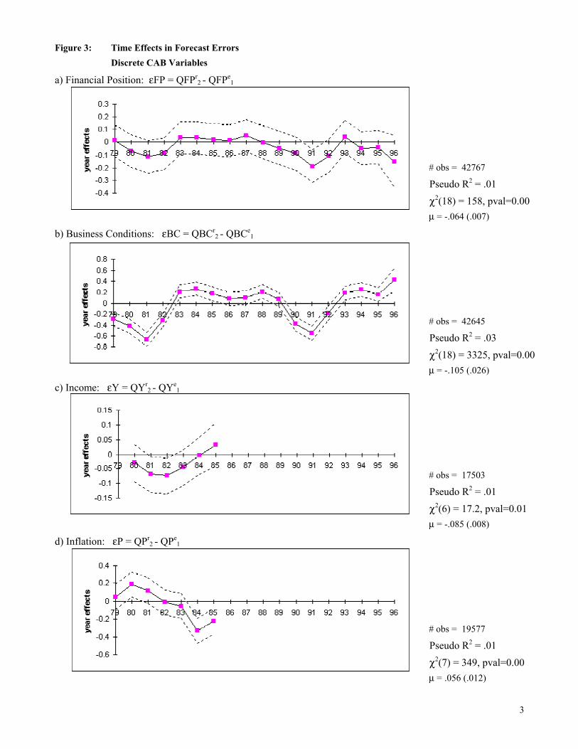
errors across households in a given month can be correlated by common shocks. In Figure 3, the

resulting estimates of µ for εFP, εBC, and εY are all significantly negative, while the average

inflation error εP is positive. (Recall that for inflation, +1 represents the bad state, the reverse of

the other variables.) Again, the realizations are disproportionately likely to be worse than

expected.

However, as suggested by the nonparametric rationality tests above, one should not

conclude from these results that people are generally over-optimistic or over-confident,

uniformly across time. One can test for significant time effects in the forecast errors ε, even

without cardinalizing them, by using ordered probits. Equation (4) was first estimated using only

the time dummies as independent variables. The resulting coefficients and standard errors are

graphed in Figure 3. For clarity year dummies are presented, but the conclusions are the same

using the full set of month dummies. For all four discrete forecast errors the chi-squared tests

indicate that the year dummies are jointly very significant. That is, there is significant variation

in households’ forecast errors from year to year. The non-price errors εFP, εBC, and εY are very

negative throughout the early 1980’s and the early 1990’s. Consistent with the results above, it

appears that people were negatively surprised by the recessions, repeatedly over their

23 E.g., one could test the rationality of binary variables such as “a) Will conditions improve or at least stay the

23

duration.24,25 However, recalling the procyclicality of sentiment in Figures 1 and 2 (in particular

the fact that QFPe is a leading indicator), one should not conclude that people altogether fail to

foresee the business cycle. Rather, it appears that people understate the amplitude or duration of

the cycle, in both downturns and upturns. Nonetheless, the pseudo R2's in Figure 3 suggest that

time effects explain only a small part of the variation in the forecast errors. The time effects are

more significant and produce a larger R2 for the forecast error for aggregate activity, εBC, than

for the household-specific errors εFP and εY.

Figure 3d) records the results for the discrete inflation forecast errors εP. The year

effects swing from positive to negative. Evidently inflation was higher than expected at the end

of the 1970’s, but then people were surprised by how quickly it abated in the early to mid

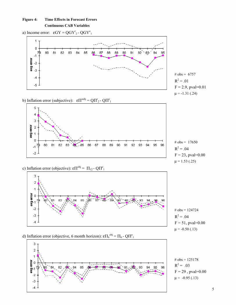
1980’s.26 Figure 4b) presents analogous results for the continuous, subjective inflation error,

εΠsubj. It too dramatically declines from positive to negative in the early 1980’s, and is positive

same, or b) will conditions worsen?” This variable would correspond to grouping the 0’s with the +1’s. 24 Under basic models of rational expectations, efficiency requires that individual agents’ forecast errors be independent across time. Even though only one forecast error is available per household, one can test for serial correlation in the aggregated forecast errors, i.e. in the estimated month dummies underlying the figures. For Figure 3, there is significant autocorrelation through 12, 20, 4, and 21 months for εFP, εBC, εY, and εP, respectively. For Figure 4 below, autocorrelation is significant through 4, 22, 21, and 11 months for εGY, εΠsubj, εΠobj, and εΠ6

obj, respectively. However, recall that tests of efficiency on aggregated data are subject to aggregation bias. 25 The overlapping forecast periods described above could generate some autocorrelation through 5 months. But Figure 3 and the results in the previous note show that the autocorrelation in the time effects lasts much longer than this. The diagrams and conclusions remain qualitatively the same on limiting the sample to non-overlapping periods as above, or on using the full set of month dummies in equation (4). Estimating (4) by OLS produces year effects that are similar in pattern and even magnitude to those in Figure 3. 26 There is a small discrepancy in the wording of QPe and QPr. QPe asks about prices in general, whereas QPr asks about the prices of goods the household itself buys. This distinction should not matter much here. First, the CAB data are representative, so the average price of goods bought should be relatively close to the consumer price level. Second, any discrepancy is unlikely to explain the dramatic shift in forecast errors from positive to negative during the disinflation in the early 1980's (Figure 3d)). Third, the continuous questions QΠe are about aggregate prices and so Figure 4c) is not subject to the discrepancy, yet yields a similar pattern. Fourth, Croushore [1998] documents a similar pattern using the aggregate time series for inflation expectations from the Livingston survey and the Survey of Professional Forecasters, where again there is no discrepancy in the wording of the survey questions. Fifth, the results are similar on using the regional CPI for the census region in which the household lives, instead of the national CPI, or using instead the PCE and GDP deflators. Finally, even though QPe doesn’t specifically mention the CPI, both the results of the previous literature and the staff at the Institute for Social Research suggest that the CPI is

24

on average over the sample. Figure 4c) shows the objective forecast error εΠobj, which uses as its

realization the actual CPI inflation rate Π12 over the next 12 months (as opposed to the

respondent-supplied QΠr used in Figure 4b), which is not available after 1985).27 The errors

again decline with the disinflation in the early 1980's. The magnitude of this decline is both

statistically and economically significant, with inflation starting about two percentage points

higher than expected in 1979 but falling 2.5 percentage points lower than expected by 1982, a

4.5 percentage point change. More recently, throughout the 1990's households were repeatedly

surprised by the low levels of inflation, by about 1 to 2 percentage points. Such negative errors

dominate in the longer sample, making the overall average error µ significantly negative for

εΠobj, whereas it was positive for εΠsubj over the shorter sample period. These results vividly

illustrate how sensitive estimates of bias can be to the sample period, even for long samples.

Figure 4d) shows the objective forecast errors εΠ6obj using instead the CPI inflation rate over

only the first six months after households’ first interviews (annualized), to see the effects of the

six-month mismatch between expectations and realizations in the other variables. Reassuringly,

the results do not much differ from Figure 4c), suggesting that the mismatch is not driving the

results.28 More generally, the results for inflation are robust across different definitions of

inflation and its forecast error.

the appropriate benchmark. The ISR surveyors prod respondents for the prices of “the things people buy,” intending to capture consumer prices, although they deliberately avoid using jargon like “CPI-U”. 27 The drawbacks to using actual inflation emphasized by Keane and Runkle [1990] do not apply here. First, unlike the GDP deflator the CPI is not revised. (The seasonal adjustment can be changed, but this is unlikely to be important. To avoid any problem the reported results use the non-seasonally-adjusted CPI. Using the seasonally adjusted CPI instead made extremely little difference.) Second, revisions are a problem only if the revised variable is used as a regressor to test efficiency but was not in agents' information sets. The efficiency tests here do not use revised variables as regressors. 28 In addition to having similar time-series properties, the cross-sectional properties of εΠ6

obj are similar to those for εΠobj in Table 2 below, both qualitatively and quantitatively. Further, their six-month difference does not materially change the Euler equation results for εΠobj below in Table 4. As for the other forecast errors, there is no reason to

25

Figure 4a) displays the forecast errors εGY for income growth, which are available only

in the later part of the sample period. Despite the larger standard errors (reflecting the smaller

sample size), the forecast errors still significantly vary over time. They start declining in 1990,

and rebound only after 1993, when income growth was 2.5 percentage points lower than

expected. Again, people seem to have been surprised by the recession, and perhaps also by the

weakness of the subsequent recovery.29,30

As a further check that the six-month timing mismatch is not driving the results, forecast

errors with the correct timing can be estimated for each household i. For each matched

expectational question Qei, the realization 12 months later $Q r

12,i can be estimated from the

corresponding realizations Qrj of other households j with the same characteristics Z that are

interviewed 12 months later. The resulting forecast errors ε12 ≡ $Q r12 - Qe

1 exhibit very similar

means and time effects as those graphed in Figures 3 and 4a-b). The other conclusions below

also persist, confirming that the timing mismatch is not a problem.31,32 Further, the consistency

believe that they would be any more sensitive to the six-month mistiming. Their Euler equation results do not qualitatively change on slightly perturbing the timing of the mapping between the CEX and CAB samples. 29 Though part of the reason εGY troughs only in 1993 might be the lag in its reference period, discussed above. 30 Again, these conclusions persist on dropping the overlapping forecast periods. The average errors µ for εΠsubj and εΠ6

obj remain significant in all six non-overlapping samples. (For εΠobj µ is less significant, but with a 12 month horizon, twice as much of the data (11/12) had to be dropped. Even so εΠobj still varies significantly over time, in all the non-overlapping samples.) For εGY µ remains significant in over half of the non-overlapping samples. To allow for one month's delay in the release of the CPI, this analysis was redone dropping 6/7 of the data for εΠ6

obj and 12/13 for εΠobj. The conclusions are the same. As already noted, the serial correlation in the aggregated inflation errors lasts well over a year. 31 Because ε12 is continuous, the estimation is by OLS. While this changes the magnitude of the time effects compared to the ordered probit time effects for ε graphed in Figure 3, the differences are small even quantitatively. Overall, the differences in the time effects for ε12 versus ε are generally comparable in scope to the differences for εΠ6

obj versus εΠobj graphed in Figures 4c) and d). The cross-sectional properties of ε12 are also similar to those for ε in Table 2. 32 The similarity of the results for ε and ε12 also suggests that recall bias is not driving the conclusions, because ε and ε12 are calculated using different realization questions with only partly overlapping reference periods. Severe recall bias would imply little overlap between these realization questions. Further, recall bias is unlikely to be correlated with monetary policy, the business cycle, and skill-biased technical change, so is unlikely to explain the results in Figures 3-5. Finally, if the systematic components in the measured forecast errors simply reflected recall bias, not actual shocks, they should not help predict consumption changes below.

26

of the results in Figures 3 and 4 suggests that the former are not driven by the discreteness of its

variables.

In sum, consumer forecasts appear to have been biased. However, it is very difficult to

distinguish whether they were biased ex ante, or just ex post, requiring many years -- even

decades -- to meet their targets on average. In either case the bias is problematic for empirical

studies with short sample periods. In particular the business cycle and inflation regime induce

low-frequency systematic patterns in forecast errors.

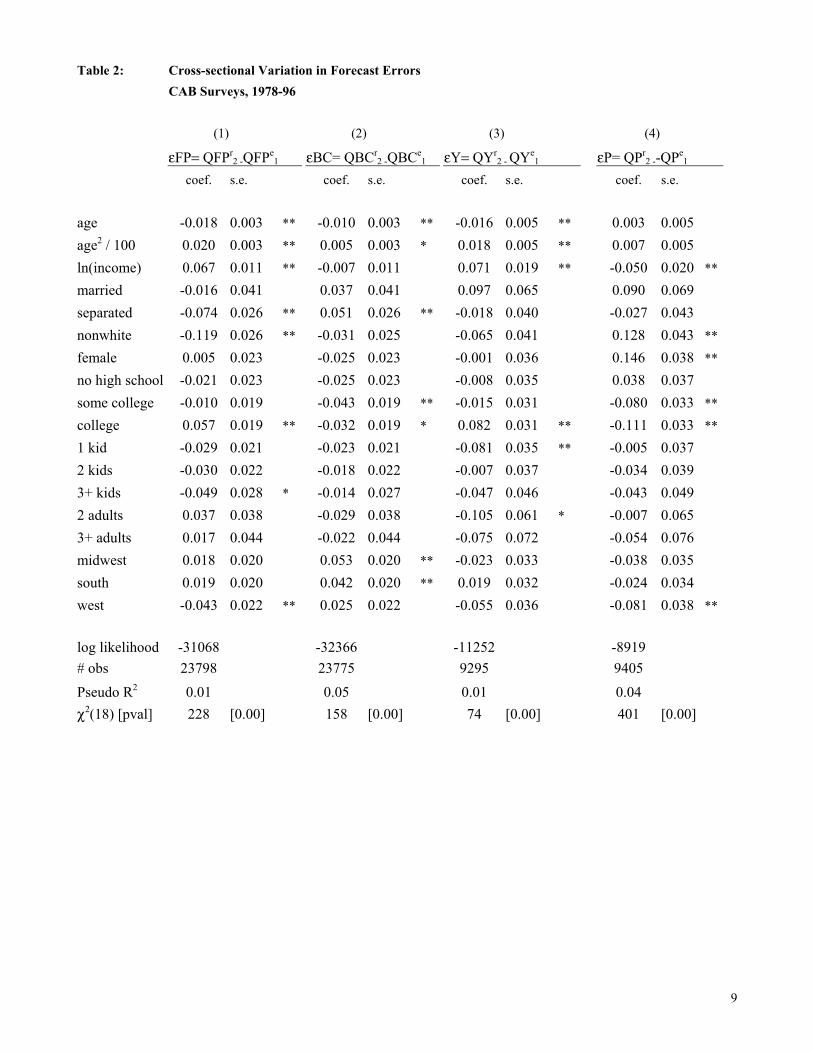
Turning to the efficiency of forecasts, the demographic variables Z were added to the

models of the forecast errors ε using equation (4), along with the full set of month dummies (but

not yet interacting age and income by month). Table 2 records the results, starting with ordered

probit models of the discrete errors in columns (1)-(4). The pseudo R2’s are small, implying that

the forecast errors are largely unsystematic, as expected. Nonetheless, according to the chi-

squared statistics the demographic variables are jointly very significant, for all four discrete

errors. While it is difficult to interpret individual coefficients in this context, there are some

interesting patterns. As regards financial position in column (1), the errors εFP tend to be more

positive on average for older, higher income, and higher education households, more negative

for divorcees and minorities. Since the overall average error µ was negative (Figure 3a), the bias

in the forecasts QFPe tends to decrease on average with age, income, and education.

The pattern of results is roughly similar for business conditions εBC and income εY in

columns (2) and (3), and often reversed in sign for inflation εP (which has the opposite coding)

in column (4). Columns (5)-(7) show analogous results for the continuous income and inflation

variables, estimated by OLS. In all cases the demographic variables are again jointly quite

significant, counter to the requirement of efficiency. They are also economically significant. For

27

instance, in column (7), the inflation forecast error is about 0.4 percentage points larger (more

negative) for those without high school education, relative to those with high school education.

The error is about 1.0 percentage point larger as real (1982-84 $) household income declines

from $50,000 to $10,000, and for minorities and females relative to whites and males.

Whether one should interpret these results as evidence of “irrationality” is a subtle issue.

It could be that young, low income, and low education people have perfectly rational

expectations ex ante, but ex post happened to have received disproportionately bad shocks over

the sample period. This is consistent with the literature finding increased inequality over the

period, in part due to skill-biased technical change (Cutler and Katz [1991], Attanasio and Davis

[1996]). But even the ex post interpretation of the results is problematic for empirical studies that

assume that time dummies capture all systematic components of forecast errors. Further, the

inefficiency of the forecasts of aggregate variables (QBC, QP, and QΠ) is harder to explain, and

more likely represents ex ante inefficiency. Even if people receive different shocks to their

income and financial position, household-specific shocks should have less effect on their

forecasts of aggregate economic activity and prices.

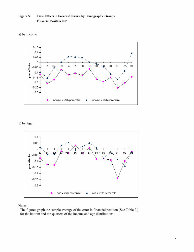
The cross-sectional distribution of forecast errors can change over time. To illustrate,

Figure 5 shows the sample average of the errors in financial position εFP, year-by-year for

different demographic groups. Since income and age are the variables interacted with time

below, the figures contrast the histories of the top and bottom quartiles of the income and age

distributions. In Figure 5a) for income, the errors are always more negative for low income

households than for high income households, though they are more cyclical for the high income

households. One interpretation is that during the expansions high income households received

relatively good shocks, but low income households continued to receive somewhat negative

28

shocks, consistent with ongoing skill-biased technical change. These results go beyond most of

the literature on technical change by implying that the increased inequality was repeatedly

unexpected, year after year, which has additional welfare consequences. In Figure 5b) for age,

the errors for young households are both more negative and more cyclical than for older

households. This suggests that both long-run and business cycle shocks disproportionately hit

young households.

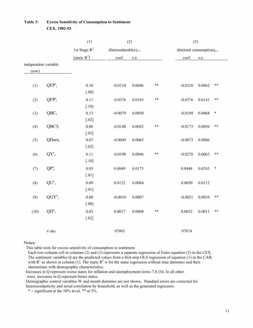
V. Results: Excess Sensitivity and Systematic Heterogeneity in Forecast Errors

Even if expectations are not fully rational, they might still help forecast spending. To test

for excess sensitivity of consumption to sentiment, the sentiment variables $Q were first imputed

into the CEX using an OLS regression of equation (1). For brevity these results are not reported,

but are available in the working-paper version.33 In this first-step most of the demographic

variables were significant, and jointly they were very significant. In Table 3, column (1) shows

the resulting adjusted R2's from the first-step regressions. More of the level of sentiment is

explained than of the forecast error (in Table 2), as expected. The dynamic variables in equation

(1), namely the month dummies and their interactions with age and income, were always

significant.34 The “static R2′s” in brackets in column (1) come from redoing the estimation

without the dynamic variables. For all the household-specific variables (QFPr, QFPe, QYe and

QGYe), the static R2 is well over half the size of the original R2, suggesting that while the

dynamic variables help explain some of the variation in sentiment, the static demographic

variables in Z are themselves quite important. The static R2’s for the aggregate variables (QBC,

33 The working paper reported the first-step results using ordered probit models for the discrete sentiment questions. Those results are qualitatively similar to the OLS results.

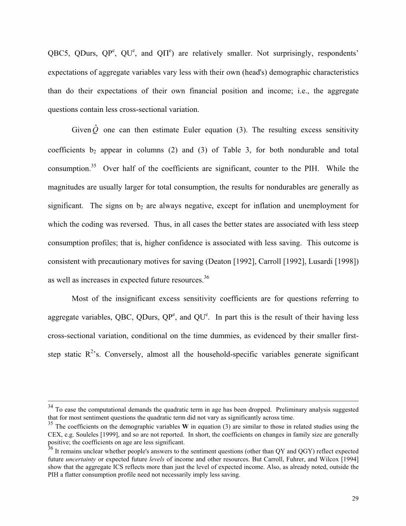
29

QBC5, QDurs, QPe, QUe, and QΠe) are relatively smaller. Not surprisingly, respondents’

expectations of aggregate variables vary less with their own (head's) demographic characteristics

than do their expectations of their own financial position and income; i.e., the aggregate

questions contain less cross-sectional variation.

Given $Q one can then estimate Euler equation (3). The resulting excess sensitivity

coefficients b2 appear in columns (2) and (3) of Table 3, for both nondurable and total

consumption.35 Over half of the coefficients are significant, counter to the PIH. While the

magnitudes are usually larger for total consumption, the results for nondurables are generally as

significant. The signs on b2 are always negative, except for inflation and unemployment for

which the coding was reversed. Thus, in all cases the better states are associated with less steep

consumption profiles; that is, higher confidence is associated with less saving. This outcome is

consistent with precautionary motives for saving (Deaton [1992], Carroll [1992], Lusardi [1998])

as well as increases in expected future resources.36

Most of the insignificant excess sensitivity coefficients are for questions referring to

aggregate variables, QBC, QDurs, QPe, and QUe. In part this is the result of their having less

cross-sectional variation, conditional on the time dummies, as evidenced by their smaller first-

step static R2’s. Conversely, almost all the household-specific variables generate significant

34 To ease the computational demands the quadratic term in age has been dropped. Preliminary analysis suggested that for most sentiment questions the quadratic term did not vary as significantly across time. 35 The coefficients on the demographic variables W in equation (3) are similar to those in related studies using the CEX, e.g. Souleles [1999], and so are not reported. In short, the coefficients on changes in family size are generally positive; the coefficients on age are less significant. 36 It remains unclear whether people's answers to the sentiment questions (other than QY and QGY) reflect expected future uncertainty or expected future levels of income and other resources. But Carroll, Fuhrer, and Wilcox [1994] show that the aggregate ICS reflects more than just the level of expected income. Also, as already noted, outside the PIH a flatter consumption profile need not necessarily imply less saving.

30

excess sensitivity.37 Thus, the cross-sectional information in sentiment appears to help predict

consumption.

There are many possible sources of this excess sensitivity. One possibility is unobserved

differences in discount factors and other household fixed effects. Following Runkle [1991],

lagged consumption growth from households’ first interview was added to equation (3) to

control for household fixed effects, at the cost of a loss of sample size and power. Nonetheless

over half of the significant coefficients for nondurable consumption in Table 3 remain

significant, including QFPe, QBC5, and QYe. While QFPr and QΠe become less significant, QPe

becomes more significant.38 Hence, heterogeneous discount factors and other fixed effects

cannot alone be generating the estimated excess sensitivity. Further, Hausman tests and

autocorrelation tests of the residuals produce little evidence for the presence of fixed effects,

consistent with the previous literature (Browning and Lusardi [1996]).39

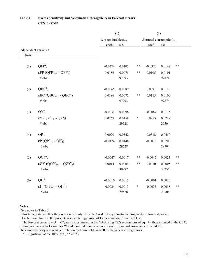
Another possible, but understudied, explanation for the results is systematic

heterogeneity in forecast errors. This is especially likely to be a problem since both sentiment

and forecast errors have just been found to be correlated with the same household demographic

37 Even though QFPr does not ask about the future, time-series studies have similarly found the coincident component of the aggregate ICS index (QFPr +QDurs) to be useful in forecasting (e.g., Throop [1992]). 38 These results do not correct the standard errors for the generated sentiment regressors, because the Angrist and Krueger [1992] estimator requires that the independent variables in equation (3) be available in the first-step dataset, but the CAB does not measure consumption growth. 39 Most studies assume that preferences are identical across agents, in which case the time dummies control for the net discount factors (r-ρ). Omitted fixed effects should lead to positive autocorrelation in the residuals of individual households’ consumption growth. However, in all regressions in Tables 3 and 4 the residuals are negatively correlated at both the first and second household lags. The Hausman test is motivated by the fact that adding lagged consumption growth provides consistency in the presence of fixed effects, but inefficiency in their absence. In 17 of the 20 Euler equations in Table 3, the Hausman test fails to find evidence for fixed effects. Also, the 3 exceptions are all for sentiment questions regarding aggregate variables (QDurs, QP, QΠ), yet it would be surprising if households’ discount factors were more correlated with aggregate sentiment questions than with household-specific sentiment questions. (Further, the excess-sensitivity coefficients for two of these exceptions, QDurs and QP, are already insignificant in Table 3, before adding lagged consumption growth. Hence their Hausman test results do not imply that failure to control for fixed effects generated any spurious excess sensitivity.) Similarly, in Table 4, most of the Hausman tests fail to find evidence for fixed effects.

31

characteristics. These findings suggest that even a long sample period and a full set of time

dummies might not be enough to ensure orthogonality of the forecast errors with the sentiment

regressors. Since the forecast errors are likely to be correlated with many regressors of interest,

this would be a general problem.

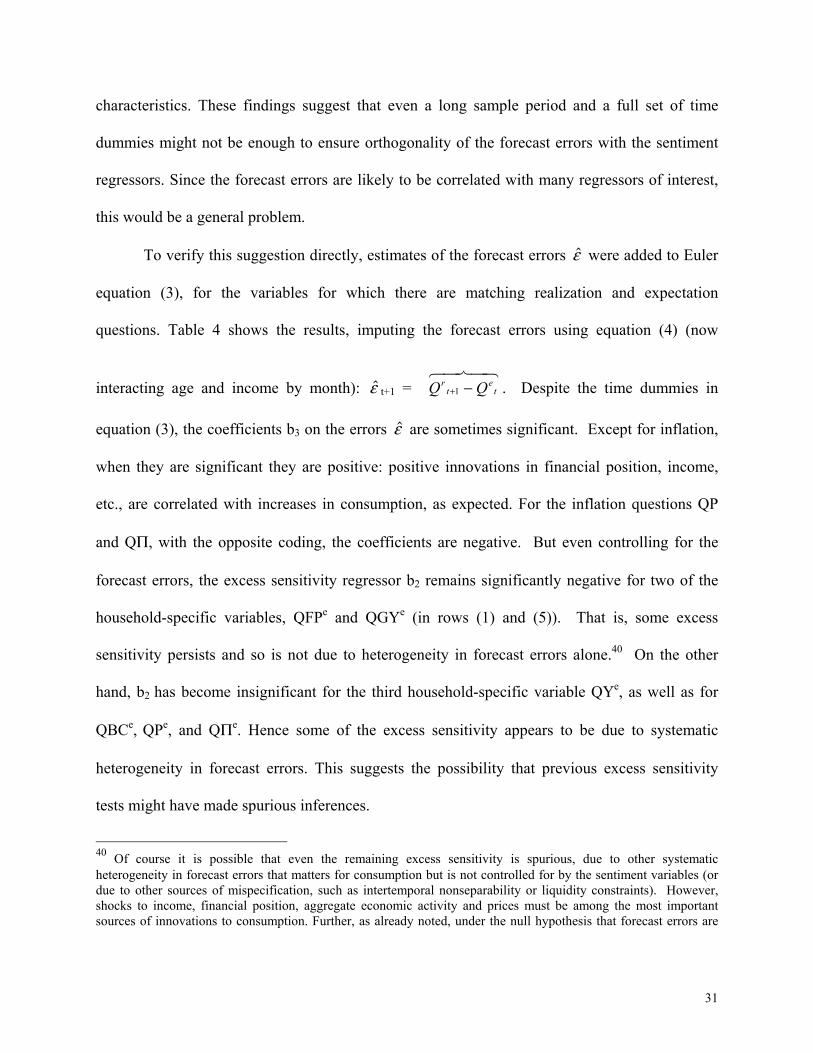
To verify this suggestion directly, estimates of the forecast errors $ε were added to Euler

equation (3), for the variables for which there are matching realization and expectation

questions. Table 4 shows the results, imputing the forecast errors using equation (4) (now

interacting age and income by month): $ε t+1 = Q Qrt

et+ −1

6 74 84. Despite the time dummies in

equation (3), the coefficients b3 on the errors $ε are sometimes significant. Except for inflation,

when they are significant they are positive: positive innovations in financial position, income,

etc., are correlated with increases in consumption, as expected. For the inflation questions QP

and QΠ, with the opposite coding, the coefficients are negative. But even controlling for the

forecast errors, the excess sensitivity regressor b2 remains significantly negative for two of the

household-specific variables, QFPe and QGYe (in rows (1) and (5)). That is, some excess

sensitivity persists and so is not due to heterogeneity in forecast errors alone.40 On the other

hand, b2 has become insignificant for the third household-specific variable QYe, as well as for

QBCe, QPe, and QΠe. Hence some of the excess sensitivity appears to be due to systematic

heterogeneity in forecast errors. This suggests the possibility that previous excess sensitivity

tests might have made spurious inferences.

40 Of course it is possible that even the remaining excess sensitivity is spurious, due to other systematic heterogeneity in forecast errors that matters for consumption but is not controlled for by the sentiment variables (or due to other sources of mispecification, such as intertemporal nonseparability or liquidity constraints). However, shocks to income, financial position, aggregate economic activity and prices must be among the most important sources of innovations to consumption. Further, as already noted, under the null hypothesis that forecast errors are

32

The forecast errors were also computed by first separately imputing the realizations and

expectations $Q rt+1 and $Q e

t in the CEX using equation (1), and then taking their difference: $ε t+1

= $Q rt+1 - $Q e

t. The results are generally similar, and appear in the working paper.41 In sum,

however one controls for the forecast errors, there remains significant excess sensitivity,

especially for the household-specific variables regarding financial position and income.

VI. Conclusion

This paper provided perhaps the first comprehensive analysis of the household data

underlying the Michigan Index of Consumer Sentiment. This data allowed for a cleaner test of

the rationality of consumers’ expectations than in most previous studies. The results can also be

interpreted as characterizing the shocks that hit different types of households over time.

Expectations appear to be biased, at least ex post, in that forecast errors did not average out even

over a sample period lasting almost 20 years. This bias is not constant over time; it is related to

the inflation regime and the business cycle. People underestimated the disinflation of the early

1980's and in the 1990's, and generally appear to underestimate the amplitude or duration of

business cycles. Expectations are also inefficient, in that people’s forecast errors are correlated

with their demographic characteristics and/or aggregate shocks did not hit all people uniformly.

For instance, during recent expansions high income households received relatively good shocks,

but low income households continued to receive somewhat negative shocks, consistent with

classical, they should be orthogonal to other factors in agents’ information sets, including discount rates. Hence the effect in Table 4 of adding forecast errors to the Euler equation cannot be due to such factors. 41 When the realization questions Qr are not available for much of the sample, the change in the estimated expectational variable was used instead: ε̂ t+1 = Q̂ e

t+1 - Q̂ et. A change in expectations over time still represents an

innovation. The results are somewhat less significant than those reported in Table 4, perhaps because the imputed variables Q̂ do not vary enough across quarters. Still, ε̂ is significantly positive for QYe. Also the excess

33

ongoing, unexpected skill-biased technical change. Whether one interprets these results as

evidence of ex ante "irrationality" or not, they are problematic for empirical studies that have

short sample periods or assume that time dummies control for all systematic components of

forecast errors. Empirical implementations of forward-looking models need to recognize that

forecast errors are more complex than usually assumed.

Attention then turned to whether the sentiment data helps predict household expenditure.

Significant evidence of excess sensitivity was found, counter to the PIH. Higher confidence was

correlated with less saving, consistent with precautionary motives and increases in expected

future resources. Further, this paper provided a unique test of the specific alternative hypothesis

that systematic heterogeneity in forecast errors explains the rejection of the PIH. Previous

studies, lacking explicit measures of these errors, have not been able to consider this hypothesis

directly. Demographic components of forecast errors were found to explain some, but not all, of

the excess sensitivity. More broadly, because forecast errors are correlated with household

demographic characteristics, they will be correlated with many regressors of interest in forward-

looking models, suggesting that non-classical forecast errors are in practice a general and

potentially serious problem. Finally, the cross-sectional variation in sentiment, net of time

dummies, was itself found to be informative. This is information lost in the aggregated ICS time

series for sentiment; nor is it contained in other macro variables used in forecasting. Of the

Michigan survey questions, those asking specifically about the household, rather than the

aggregate economy, were generally found to contain the most useful cross-sectional information.

This analysis can be extended in a number of ways. First, given the significance of the

cross-sectional distribution of sentiment, new sentiment time series might be created to better

sensitivity coefficients b2 for QFPe and QGYe remain significant, and now are significant for QYe. Again the excess

34

incorporate this distribution, for instance by taking weighted averages of sentiment across

households.42 Second, one can similarly examine many other economic decisions in addition to

spending for which expectations matter, as in the portfolio study of Souleles [2001]. Cross-

sectional data is especially well suited to studying the effects of one-time events, like the 1987

stock market crash. Third, durables purchases might be modeled more explicitly, taking into

account their discreteness.

sensitivity coefficients are generally insignificant for the aggregate variables, with the exception of QΠe. 42 The weights could reflect e.g. the scale of spending by different groups of people, or the sensitivity of their spending to their sentiment.

35

VII. Data Appendix

A. The CAB survey.

The additional sentiment questions, not part of the ICS, include the following:

QBCr. Would you say that at the present time business conditions are better or worse than they were a year ago? [better now, about same, worse now]

QBCe. And how about a year from now, do you expect that in the country as a whole, business conditions will be better or worse than they are at present, or just about the same? [better a year from now, about same, worse a year from now]

QYr. During the last year or two, would you say that your (family) income went up more than prices, went up about the same as prices, or went up less than prices? [more, same, less]

QYe. During the next year or two, do you expect that your (family) income will go up more than prices will go up, about the same, or less than prices will go up? [more, same, less]

QPr. During the last 12 months, have prices of the things you buy remained unchanged, or have they gone up, or have they gone down? [gone up, remained unchanged, gone down]

QPe. During the next 12 months, do you think that prices in general will go up, or down, or stay where they are now? [go up, will not go up, go down]

QUe. How about people out of work during the coming 12 months—do you think that there will be more unemployment than now, about the same, or less? [more, about same, less]

QGYr. [The growth rate is computed from changes in the level of income from the following question:] Now, thinking about your (family's) total income from all sources (including your job), how much did you (your family) receive in [the previous calendar year]?

QGYe. By what percent do you expect your (family) income to (increase/decrease) during the next 12 months?

QΠr. By about what percent do you think prices have gone (up/down) on the average, during the last 12 months?

QΠe. By about what percent do you expect prices to go (up/down) on the average, during the next 12 months?

Other answers such as “Don’t Know” are also allowed, but are not used here. When the answers

to QΠ and QGY were topcoded, they were not used.

For CAB interviews that took place in more than one installment, if these installments

spanned two different calendar months, the second month is used to date the observation. If any

demographic variable used in a regression is missing, topcoded, or flagged (e.g., "Don’t Know"),

the observation is not used. For the demographic variables Z, when the continuous measure of

total household income was missing, the midpoint of the bracketed income variable was used

instead. (But the bracketed variable is not used in computing the growth rate of income.) The

reference period for realized income (used in computing the growth rate QGYr) is the previous

calendar year, whereas for the CEX it is the past 12 months. For consistency CAB income was

deflated using the CPI (1982-84 $) for the past 12 months. Since the original CAB income

variable is constrained to be positive, for consistency total income in the CEX was used only

36

when positive and not flagged. Sample selection is discussed in the text.

B. The CEX.

In aggregating individual expenditures, if any component of total consumption or

nondurable consumption was topcoded or missing its cost, the whole consumption group was set

to missing. If any component was missing its date or dated before the reference period, the

group was dropped for all interviews for the household at issue. A large number of expenditures

are dated in the month of the interview. Following the recommendation of the staff at the BLS,

for consistency such expenditures were accrued to the following reference period.

In addition to the sample restrictions in the text, an observation is dropped if the age of

the head increases by more than one, or decreases, on moving into the next quarter. An

observation is also dropped if the age of any other member changes in this way and thereby

results in the member's switching between being a kid (less than 16 years old) and an adult (at

least 16). If any variable used in a regression is missing, the observation is not used. Other

sample restrictions are described in the text.

37

References Acemoglu, D., and Scott, A., 1994, “Consumer Confidence and Rational Expectations: Are Agents’ Beliefs Consistent with the Theory?” Economic Journal, 104, pp. 1-19. Alessie, R. and Lusardi, A., 1997, “Saving and income smoothing: Evidence from panel data”, European Economic Review, 41, pp. 1251-1279. Angrist, J. and Krueger, A., 1992, “The Effect of Age at School Entry on Educational Attainment: An Application of Instrumental Variables with Moments from Two Samples”, Journal of the American Statistical Association, 87, pp. 328-336. Attanasio, O., and Davis, S., 1996, "Relative Wage Movements and the Distribution of Consumption," Journal of Political Economy, 104(6), December, pp. 1227-62. Attanasio, O., and Weber, G., 1995, "Is Consumption Growth Consistent with Intertemporal Optimization? Evidence from the Consumer Expenditure Survey," Journal of Political Economy, 95, pp. 1121-1157. Batchelor, R., 1986, “Quantitative v. Qualitative Measures of Inflation Expectations,” Oxford Bulletin of Economic and Statistics, 48, pp. 99-120. Batchelor, R., and Jonung, L., 1989, “Cross-Sectional Evidence on the Rationality of the Mean and Variance of Inflation Expectations,” in Grunert, Klaus G., ed., 1989, Understanding Economic Behavior, Boston: Kluwer press, pp. 93-105. Browning, M., and Lusardi, A., 1996, “Household Saving: Micro Theories and Micro Facts,” Journal of Economic Literature, v34, December, pp. 1797-1855. Burch, S., and Gordon, S., 1985, “The Problem of Inference in Consumer Surveys,” Federal Reserve Board of Governors working paper, May. Carroll, C., 1992, “The Buffer-Stock Theory of Saving: Some Macroeconomic Evidence,” Brookings Papers on Economic Activity, 2, pp. 61-156. Carroll, C., Fuhrer, J., and Wilcox, D., 1994, “Does Consumer Sentiment Forecast Household Spending? If So, Why?,” American Economic Review, 84, pp. 1397-1408. Carroll, C., Dynan, K., and Krane, S., 1996, “Balance Sheets and Precautionary Saving,” Federal Reserve Board of Governors working paper, January. Chamberlain, G., 1984, "Panel Data," in Griliches, Z., and Intriligator, M., Handbook of Econometrics, Amsterdam: North-Holland. Croushore, D., 1998, "Evaluating Inflation Forecasts," Federal Reserve Bank of Philadelphia working paper, June.

38

Cutler, D., and Katz, L., 1991, “Macroeconomic Performance and the Disadvantaged,” Brookings Papers on Economic Activity, 0(2), pp. 1-61. Das, M., Dominitz, J., and van Soest, A., 1999, “Comparing Predictions and Outcomes: Theory and Application to Income Changes,” Journal of the American Statistical Association, 94, March, pp. 75-85. Das, M., and van Soest, A., 1999, “A Panel Data Model for Subjective Information on Household Income Growth,” Journal of Economic Behavior and Organization, 40, pp. 409-426. Deaton, A., 1992, Understanding Consumption, Oxford: Oxford University Press.

Dominitz, J., 1993, “Subjective Expectations of Unemployment, Earnings, and Income,” University of Wisconsin-Madison working paper, November. Dynan, K., 1993, “How Prudent Are Consumers?” Journal of Political Economy, 101, December, pp. 1104-13. Flavin, M., 1991, “The Joint Consumption/Assets Demand Decision: A Case Study in Robust Estimation,” NBER working paper #3802. Friend, I., and Adams, G., 1964, “The Predictive Ability of Consumer Attitudes, Stock Prices, and Non-Attitudinal Variables,” Journal of the American Statistical Association, 59, December, pp. 987-1005. Gramlich, E., 1983, “Models of Inflation Expectations Formation,” Journal of Money, Credit, and Banking, 15, pp. 155-173. Hall, R., and Mishkin, F., 1982, "The Sensitivity of Consumption to Transitory Income: Estimates from Panel Data on Households," Econometrica, 50, March, pp. 461-82. Jappelli, T., Pischke, S., and Souleles, N., 1998. “Testing for Liquidity Constraints in Euler Equations with Complementary Data Sources,” The Review of Economics and Statistics, 80(2), pp. 251-262. Keane, M., and Runkle, D., 1990, “Testing the Rationality of Price Forecasts: New Evidence from Panel Data,” American Economic Review, 80, pp. 714-735. Ludvigson, S., 1996, “Consumer Sentiment and Household Expenditure: Reevaluating the Forecasting Equations,” Federal Reserve Bank of New York working paper, November. Lusardi, A., 1996, "Permanent Income, Current Income and Consumption: Evidence from Two Panel Data Sets," Journal of Business and Economic Statistics, 14, pp. 81-90. Lusardi, A., 1998, "On the Importance of the Precautionary Saving Motive," American

39

Economic Review, May. Maddala, G., Fishe, R., and Lahiri, K., 1981, “A Time Series Analysis of Popular Expectations Data,” in Zellner, A., ed., 1983, Applied Time Series Analysis of Economic Data, U.S. Department of Commerce, pp. 278-290. Mariger, R., and Shaw, K., 1993, “Unanticipated Aggregate Disturbances and Tests of the Life-Cycle Consumption Model Using Panel Data,” Review of Economics and Statistics, pp. 48-56. McNeil, J., 1974, “Federal Programs to Measure Consumer Purchase Expectations, 1946-1973: A Post-Mortem,” Journal of Consumer Research, 1, pp. 1-10. Nicholson, S., and Souleles, N., 2001, “Physician Income Prediction Errors: Sources and Implications for Behavior,” University of Pennsylvania working paper. Nicholson, S., and Souleles, N., 2001, “Physician Income Expectations and Specialty Choice,” University of Pennsylvania working paper. Runkle, D., 1991, “Liquidity Constraints and the Permanent-income Hypothesis,” Journal of Monetary Economics, 27, pp. 73-98. Shapiro, M. and Slemrod, J., 1995, "Consumer Response to the Timing of Income: Evidence from a Change in Tax Withholding." American Economic Review, 85(1), March, pp. 274-283. Souleles, N., 1999, “The Response of Household Consumption to Income Tax Refunds,” American Economic Review, forthcoming. Souleles, N., 2001, “Household Securities Purchases, Transactions Costs, and Hedging Motives,” University of Pennsylvania working paper, August. Thomas, L., 1999, “Survey Measures of Expected U.S. Inflation,” Journal of Economic Perspectives, 13(4), pp. 125-144. Throop, A., 1992, “Consumer Sentiment: Its Causes and Effects,” Economic Review, 1, Federal Reserve Bank of San Francisco, pp. 35-59. Zeldes, S., 1989, "Consumption and Liquidity Constraints: An Empirical Investigation," Journal of Political Economy, 97, pp. 305-346.

1

2

3

Figure 3: Time Effects in Forecast Errors Discrete CAB Variables a) Financial Position: εFP = QFPr

2 - QFPe1

# obs = 42767 Pseudo R2 = .01 χ2(18) = 158, pval=0.00 µ = -.064 (.007) b) Business Conditions: εBC = QBCr

2 - QBCe1

# obs = 42645 Pseudo R2 = .03 χ2(18) = 3325, pval=0.00 µ = -.105 (.026) c) Income: εY = QYr

2 - QYe1

# obs = 17503 Pseudo R2 = .01 χ2(6) = 17.2, pval=0.01 µ = -.085 (.008) d) Inflation: εP = QPr

2 - QPe1

# obs = 19577 Pseudo R2 = .01 χ2(7) = 349, pval=0.00 µ = .056 (.012)

4

Notes: · For variable and sample definitions see the notes for Table 2. · The graphed results come from an ordered probit of the forecast errors ε in {-2,-1,0,1,2} on year dummies. The middle line gives the estimated coefficients on the year dummies (in the latent index function). The outside dashed lines represent 95% confidence intervals. χ2 tests the joint significance of the year effects. · To calculate the mean forecast error µ, the errors ε are regressed by OLS on a constant, correcting the standard errors for heteroscedasticity and cross-correlation within the month.

5

Figure 4: Time Effects in Forecast Errors Continuous CAB Variables a) Income error: εGY = QGYr

2 - QGYe1

# obs = 6757 R2 = .01 F = 2.9, pval=0.01 µ = -1.31 (.24) b) Inflation error (subjective): εΠsubj = QΠr

2 - QΠe1

# obs = 17650 R2 = .04 F = 23, pval=0.00 µ = 1.53 (.25) c) Inflation error (objective): εΠobj = Π12 - QΠe

1 # obs = 124724 R2 = .04 F = 51, pval=0.00 µ = -0.50 (.13) d) Inflation error (objective, 6 month horizon): εΠ6

obj = Π6 - QΠe1

# obs = 125178 R2 = .03 F = 29 , pval=0.00 µ = -0.95 (.13)

6

Notes: · For variable and sample definitions see the notes for Table 2. · The graphed results come from an OLS regression of the forecast errors ε on year dummies, correcting the standard errors for heteroscedasticity and cross-sectional correlation within the month. The middle line records the year effects, the outside dashed lines the 95% confidence intervals. F tests the joint significance of the year effects. · To calculate the mean forecast error µ, the errors ε are regressed by OLS on a constant, correcting the standard errors for heteroscedasticity and cross-correlation within the month.

7

Figure 5: Time Effects in Forecast Errors, by Demographic Groups Financial Position εFP a) by Income b) by Age Notes: · The figures graph the sample average of the error in financial position (See Table 2.) for the bottom and top quarters of the income and age distributions.

8

Table 1: Sample Means 1982-1993 CAB CEX

age 45.5 48.7

ln(income) 9.93 9.97

married 0.567 0.583

separated 0.269 0.288

nonwhite 0.093 0.116

female head 0.252 0.282

no high school 0.165 0.243

some college 0.261 0.217

college 0.279 0.237

1 kid 0.154 0.155

2 kids 0.150 0.145

3+ kids 0.081 0.083

2 adults 0.526 0.552

3+ adults 0.101 0.125

midwest 0.284 0.262

south 0.322 0.287

west 0.201 0.237 # obs 54488 97993 Notes: · The omitted categorical variables are: single, white, male head, high school graduate, no kids, one adult, northeast. Income is real household income (1982-84 $). · For comparison the CAB sample period is restricted to the CEX sample period, 1982-93. The actual samples used in the different analyses in the paper can differ somewhat due to missing data or additional sample restrictions, as explained in the text and the following tables.

9

Table 2: Cross-sectional Variation in Forecast Errors CAB Surveys, 1978-96 (1) (2) (3) (4)

εFP= QFPr2 -QFPe

1 εBC= QBCr2 -QBCe

1 εY= QYr2 - QYe

1 εP= QPr2 --QPe

1 coef. s.e. coef. s.e. coef. s.e. coef. s.e.

age -0.018 0.003 ** -0.010 0.003 ** -0.016 0.005 ** 0.003 0.005 age2 / 100 0.020 0.003 ** 0.005 0.003 * 0.018 0.005 ** 0.007 0.005 ln(income) 0.067 0.011 ** -0.007 0.011 0.071 0.019 ** -0.050 0.020 **

married -0.016 0.041 0.037 0.041 0.097 0.065 0.090 0.069 separated -0.074 0.026 ** 0.051 0.026 ** -0.018 0.040 -0.027 0.043

nonwhite -0.119 0.026 ** -0.031 0.025 -0.065 0.041 0.128 0.043 **

female 0.005 0.023 -0.025 0.023 -0.001 0.036 0.146 0.038 **

no high school -0.021 0.023 -0.025 0.023 -0.008 0.035 0.038 0.037

some college -0.010 0.019 -0.043 0.019 ** -0.015 0.031 -0.080 0.033 **

college 0.057 0.019 ** -0.032 0.019 * 0.082 0.031 ** -0.111 0.033 **

1 kid -0.029 0.021 -0.023 0.021 -0.081 0.035 ** -0.005 0.037

2 kids -0.030 0.022 -0.018 0.022 -0.007 0.037 -0.034 0.039

3+ kids -0.049 0.028 * -0.014 0.027 -0.047 0.046 -0.043 0.049

2 adults 0.037 0.038 -0.029 0.038 -0.105 0.061 * -0.007 0.065

3+ adults 0.017 0.044 -0.022 0.044 -0.075 0.072 -0.054 0.076

midwest 0.018 0.020 0.053 0.020 ** -0.023 0.033 -0.038 0.035

south 0.019 0.020 0.042 0.020 ** 0.019 0.032 -0.024 0.034

west -0.043 0.022 ** 0.025 0.022 -0.055 0.036 -0.081 0.038 ** log likelihood -31068 -32366 -11252 -8919 # obs 23798 23775 9295 9405

Pseudo R2 0.01 0.05 0.01 0.04 χ2(18) [pval] 228 [0.00] 158 [0.00] 74 [0.00] 401 [0.00]

10

Table 2: Cross-sectional Variation in Forecast Errors (ctd)

CAB Surveys, 1978-96

(5) (6) (7)

εGY= GYr2 -QGYe

1 εΠsubj= QΠr2-QΠe

1 εΠobj = Π12-QΠe1

coef. s.e. coef. s.e. coef. s.e. age 0.754 0.147 ** -0.029 0.050 -0.037 0.013 **

age2 / 100 -0.675 0.142 ** 0.106 0.052 ** 0.071 0.013 ** ln(income) -5.291 0.705 ** -0.370 0.221 * 0.539 0.053 ** married 2.111 2.106 -0.226 0.609 -0.165 0.123 separated -1.167 1.240 -0.067 0.416 0.123 0.114 nonwhite -1.289 1.261 0.126 0.535 -0.815 0.140 ** female -1.360 1.075 1.032 0.338 ** -0.970 0.098 ** no high school -0.970 1.169 -0.337 0.391 -0.396 0.112 ** some college 1.234 0.816 -0.051 0.297 0.269 0.073 ** college 1.303 0.837 -0.336 0.250 0.099 0.067 1 kid -0.634 0.963 -0.361 0.308 -0.152 0.086 * 2 kids 0.194 0.962 0.017 0.341 -0.319 0.086 ** 3+ kids -0.416 1.186 -0.304 0.431 -0.504 0.120 ** 2 adults -0.007 1.945 0.822 0.552 0.097 0.108 3+ adults -1.093 2.173 1.271 0.624 ** 0.026 0.128 midwest 0.012 0.844 -0.532 0.295 * 0.116 0.081 south -1.167 0.860 -0.215 0.306 0.001 0.081 west -1.577 0.939 * -0.531 0.328 * -0.237 0.086 ** # obs 4856 8788 60695

R2 0.03 0.05 0.05 F [pval] 5.52 [0.00] 9.51 [0.00] 35.3 [0.00] Notes: · This table estimates the systematic demographic components of forecast errors ε. using Equation (4). In columns (1)-(4) the forecast errors are discrete and the estimation is by ordered probit. Qe

1 represents an expectation from interview one, Qr2 the corresponding realization from interview two. Except for

inflation, Q=+1 represents the better states (e.g. "better" or "good"), 0 the intermediate states, -1 the worse states. Forecast errors are the difference between expectations and realizations: ε = (Qr

2 - Qe1), with values in {-2,-1,0,1,2}.

In columns (5)-(7) the forecast errors are constructed analogously but are continuous. Estimation is by OLS, correcting the standard errors for heteroscedasticity. · Coefficients on month dummies are not shown. The omitted categorical variables are: single, white, male head, high school graduate, no kids, one adult, northeast. · χ2 and F test the joint significance of the demographic variables, with p-values in the brackets. * = significant at the 10% level, ** at 5%. · In columns (1)-(6) the sample is limited to households interviewed twice. Further, the same person (either head or spouse) must have been the respondent in both interviews. In column (7), which uses the actual CPI Π12 as the realization, the household may have been interviewed only once; and if interviewed twice, the respondent need not be the same person in both interviews.

11

Table 3: Excess Sensitivity of Consumption to Sentiment CEX, 1982-93 (1) (2) (3)

1st Stage R2 ∆ln(nondurables)t+1 ∆ln(total consumption)t+1 [static R2] coef. s.e. coef. s.e. independent variable

(row)

(1) QFPrt 0.10 -0.0134 0.0046 ** -0.0210 0.0062 **

[.08] (2) QFPe

t 0.11 -0.0376 0.0103 ** -0.0376 0.0141 ** [.10]

(3) QBCt 0.13 -0.0079 0.0050 -0.0109 0.0068 * [.02]

(4) QBC5t 0.06 -0.0148 0.0042 ** -0.0173 0.0056 ** [.03]

(5) QDurst 0.07 -0.0049 0.0065 -0.0073 0.0086 [.02]

(6) QYet 0.11 -0.0190 0.0046 ** -0.0278 0.0063 **

[.10] (7) QPe

t 0.05 0.0049 0.0173 0.0448 0.0243 * [.01]

(8) QUet 0.09 0.0132 0.0084 0.0050 0.0112

[.01] (9) QGYe

t 0.08 -0.0010 0.0007 -0.0021 0.0010 ** [.08]

(10) QΠet 0.03 0.0017 0.0008 ** 0.0032 0.0011 **

[.02]

# obs 97993 97874 Notes: · This table tests for excess sensitivity of consumption to sentiment. Each row-column cell in columns (2) and (3) represents a separate regression of Euler equation (3) in the CEX. The sentiment variables Q are the predicted values from a first-step OLS regression of equation (1) in the CAB, with R2 as shown in column (1). The static R2 is for the same regression without time dummies and their interactions with demographic characteristics. · Increases in Q represent worse states for inflation and unemployment (rows 7,8,10). In all other rows, increases in Q represent better states. · Demographic control variables W and month dummies are not shown. Standard errors are corrected for heteroscedasticity and serial correlation by household, as well as the generated regressors. * = significant at the 10% level, ** at 5%.

12

Table 4: Excess Sensitivity and Systematic Heterogeneity in Forecast Errors CEX, 1982-93 (1) (2) ∆ln(nondurables)t+1 ∆ln(total consumption)t+1 coef. s.e. coef. s.e. independent variables

(row)

(1) QFPet -0.0374 0.0105 ** -0.0375 0.0142 **

εFP (QFPrt+1 - QFPe

t) 0.0186 0.0075 ** 0.0105 0.0101 # obs 97993 97874

(2) QBCe

t -0.0065 0.0089 0.0091 0.0119 εBC (QBCr

t+1 - QBCet) 0.0186 0.0072 ** 0.0115 0.0100

# obs 97993 97874

(3) QYet -0.0031 0.0098 -0.0087 0.0135

εY (QYrt+1 - QYe

t) 0.0269 0.0158 * 0.0255 0.0219 # obs 29528 29504

(4) QPe

t 0.0020 0.0342 0.0318 0.0450 εP (QPr

t+1 - QPet) -0.0124 0.0148 -0.0033 0.0200

# obs 29528 29504

(5) QGYet -0.0047 0.0017 ** -0.0045 0.0023 **

εGY (QGYrt+1 - QGYe

t) 0.0014 0.0004 ** 0.0010 0.0005 ** # obs 30292 30255

(6) QΠet -0.0010 0.0015 -0.0001 0.0020

εΠ (QΠrt+1 - QΠe

t) -0.0024 0.0013 * -0.0035 0.0018 ** # obs 29528 29504 Notes: · See notes to Table 3. · This table tests whether the excess sensitivity in Table 3 is due to systematic heterogeneity in forecast errors. Each row-column cell represents a separate regression of Euler equation (3) in the CEX. The forecast errors ε = Qr

t+1-Qet are first estimated in the CAB using OLS regressions of eq. (4), then imputed in the CEX.

· Demographic control variables W and month dummies are not shown. Standard errors are corrected for heteroscedasticity and serial correlation by household, as well as the generated regressors. * = significant at the 10% level, ** at 5%.