Consumption-based Equity Valuation Christian Bach and Peter Ove Christensen

Journal article (Post print version)

CITE: Consumption-based Equity Valuation. / Bach, Christian; Christensen, Peter O. In: Review of Accounting Studies, Vol. 21, No. 4, 2016, p. 1149-1202.

The final publication is available at Springer via http://dx.doi.org/10.1007/s11142-016-9358-y

Uploaded to @CBS: June 2017

Consumption-based equity valuation∗

Christian Bach

Danske Commodities

Denmark

Peter O. Christensen†

Department of Finance

Copenhagen Business School, Denmark

April 4, 2016

Forthcoming in Review of Accounting Studies

∗We thank seminar participants at Aarhus University, London Business School, the Eighth AccountingResearch Workshop in Basel 2013, and especially Jim Ohlson (editor) and two anonymous referees for helpfulcomments. In addition, we are grateful for detailed comments and suggestions from Bent Jesper Christensen,Mateusz P. Dziubinski, Hans Frimor, Bjørn N. Jørgensen, Claus Munk, Stephen H. Penman, and ScottRichardson. We gratefully acknowledge research support from CREATES (funded by the Danish NationalResearch Foundation), D-CAF, Columbia University, and the Danish Social Science Research Council.

†Corresponding author: Peter O. Christensen, Department of Finance, Copenhagen Business School,Solbjerg Plads 3, DK-2000 Frederiksberg, Denmark; email: poc.fi@cbs.dk.

Abstract

Using a CCAPM-based risk-adjustment model, we perform yearly valuations of a large

sample of stocks listed on NYSE, AMEX, and NASDAQ over a 30-year period. The

model differs from standard valuation models in the sense that it adjusts forecasted

residual income for risk in the numerator rather than through a risk-adjusted cost of

equity in the denominator. The risk adjustments are derived based on assumptions

about the time-series properties of residual income returns and aggregate consumption

rather than on historical stock returns. We compare the performance of the model

with several implementations of standard valuation models, both in terms of median

absolute valuation errors (MAVE) and in terms of excess returns on simple investment

strategies based on the differences between model and market prices.

The CCAPM-based valuation model yields a significantly lower MAVE than the

best performing standard valuation model. Both types of models can identify invest-

ment strategies with subsequent excess returns. The CCAPM-based valuation model

yields time-series of realized hedge returns with more and higher positive returns and

fewer and less negative returns compared with the time-series of realized hedge returns

based on the best performing standard valuation model for holding periods from one

to five years. In a statistical test of one-year-ahead excess return predictability based

on the models’ implied pricing errors, the CCAPM-based valuation model is selected

as the better model.

Using the standard series of aggregate consumption and the nominal price index,

a reasonable level of relative risk aversion, and calibrated growth rates in the contin-

uing value at each valuation date, the CCAPM-based valuation model produces small

risk adjustments to forecasted residual income and low continuing values. Compared

with standard valuation models, it relies less on estimated parameters and speculative

elements when aggregating residual earnings forecasts into a valuation.

JEL Classifications: C22, C32, C51, C53, G11, G12, G14, G32.

Keywords: Equity valuation, residual income, risk-adjusted discounting, CAPM, CCAPM.

1 Introduction

Making comprehensive valuations of equities remains a challenge both in practice and in the-

ory. We do have models like the CAPM or Fama-French models to determine a risk-adjusted

cost of capital used to discount expected future residual income, but these models are typi-

cally quite imprecise when applied. The valuations obtained are very sensitive to estimates

of betas and market (factor) risk premiums. This sensitivity is due to the estimated risk

premium being compounded through the discount factor leading to exponentially increasing

risk adjustments to expected future residual income. This pattern of risk adjustments is

justified if all shocks to residual income are fully persistent on a percentage basis, i.e., if

residual income follows a geometric Brownian motion. However, if residual income contains

both persistent and transitory shocks implying processes with mean reversion, then expo-

nentially increasing risk adjustments through a constant risk premium in the risk-adjusted

cost of capital are likely to be grossly overstated. There is overwhelming evidence of mean

reversion in residual income for most firms and industries (e.g., Nissim and Penman 2001).

This is the strong force of competition, real options to expand and abandon, and entry and

exit in product markets at work.

In this article, we perform yearly valuations of a large sample of companies listed on

NYSE, AMEX, and NASDAQ over a 30-year period using a Consumption-based Capital As-

set Pricing Model (CCAPM) for risk adjustment. The model separates discounting for time

in the denominator (through a readily observable term structure of risk-free interest rates)

from discounting for risk in the numerator. This separation allows us to model the time-series

properties of firms’ residual income as mean-reverting processes. We assume residual income

follows a first-order autoregressive process, while aggregate consumption and inflation follow

geometric Brownian motions with constant expected growth rates. This allows us to derive

closed-form expressions for the model-implied risk adjustment to forecasted residual income

in the numerator.

We compare the performance of the CCAPM-based valuation model with the performance

of a large variety of implementations of the standard CAPM and three-factor Fama-French

based valuation models, with the latter type of models adjusting for risk through a risk-

adjusted cost of equity in the denominator. Model performance is measured along two

dimensions: (a) the efficient market perspective—is the model able to fit the cross-section

of stock prices as well as the level of stock prices across business cycles?—and (b) the

fundamental valuation perspective—is the model able to identify “cheap” and “expensive”

stocks?

Along the first dimension, model values are compared with the market prices of stocks.

1

Using calibrated growth rates in the continuing value at each valuation date common to all

firms in the sample, the best performing implementation of the standard valuation model

produces a median absolute valuation error (MAVE) of 36%, while the CCAPM-based val-

uation model yields a MAVE of 23%.

Along the second dimension, a simple buy-and-hold investment strategy analysis is per-

formed. At each valuation date and for each valuation model, the stocks are placed in equally

weighted buy, hold, and sell portfolios based on whether the model suggests that the stocks

are cheap or expensive. The performance of the portfolios is measured by a large set of

alternative performance measures based on subsequent (i.e., out-of-sample) returns.1 Both

types of models can identify investment strategies with subsequent excess returns.2 The

CCAPM-based valuation model yields time-series of realized hedge returns with more and

higher positive returns and fewer and less negative returns compared with the time-series of

realized hedge returns based on the best performing standard valuation model, i.e., higher

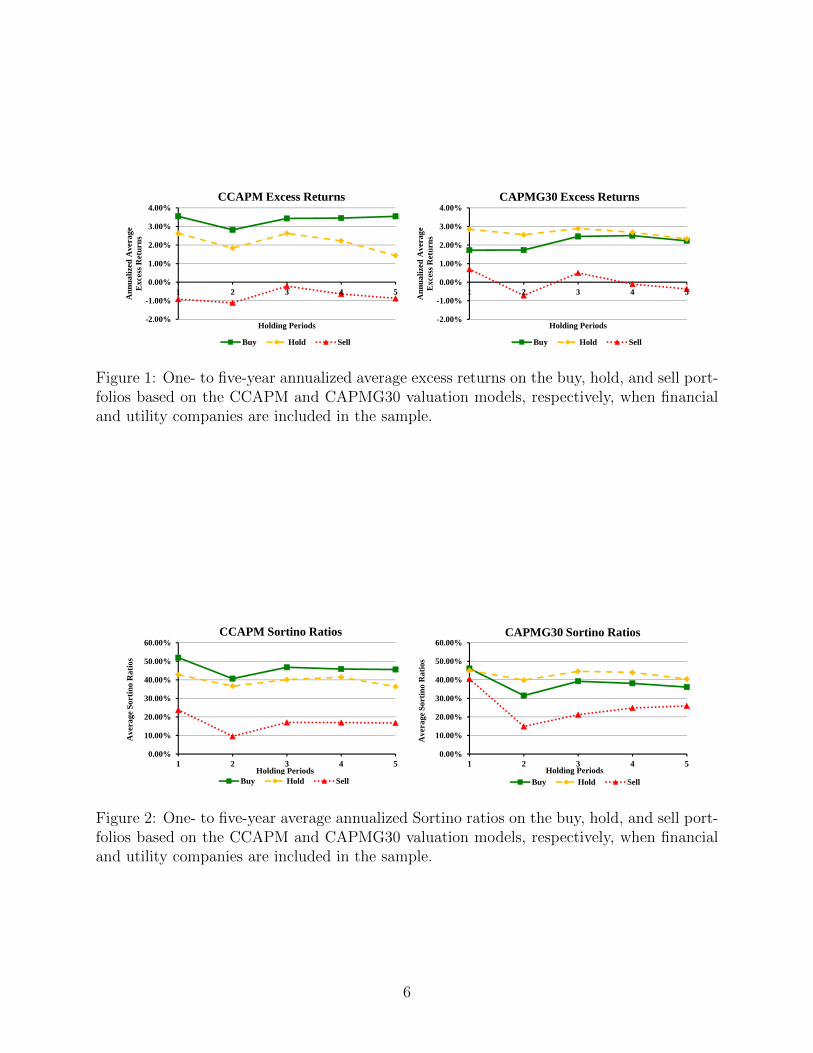
average realized returns (4.5% versus 3.0%) and higher average Sortino ratios (78% versus

34%) for holding periods from one to five years. In a statistical test of one-year-ahead ex-

cess return predictability based on the models’ implied pricing errors, the CCAPM-based

valuation model is selected as the better model with a p-value of 0.0077.

Our implementations of the residual income valuation models are based on analysts’

consensus forecasts of earnings up to five years ahead from the I/B/E/S database and an

assumption of constant payout ratios to generate implied forecasts of residual income. The

key difference between the implementations of the CCAPM-based and the standard valuation

models is how these residual income forecasts are aggregated into a valuation.

Using standard estimation procedures, the median estimated risk premium (i.e., beta

times the geometric equity premium relative to short-term Treasuries) is 6–7% for the stan-

dard valuation models, and the median calibrated growth rate in the continuing value (at

year five) to match the level of stock prices at each valuation date is close to 5%. In other

words, both the estimated risk premiums and the continuing values play important roles in

aggregating analysts’ forecasts into a valuation using standard valuation models.

Betas and equity premiums are hard to estimate reliably even if the CAPM or the Fama-

French model is the true model. As Penman (2007, page 691) states it:

“Compound the error in beta and the error in the risk premium and you have a

considerable problem. The CAPM, even if true, is quite imprecise when applied.

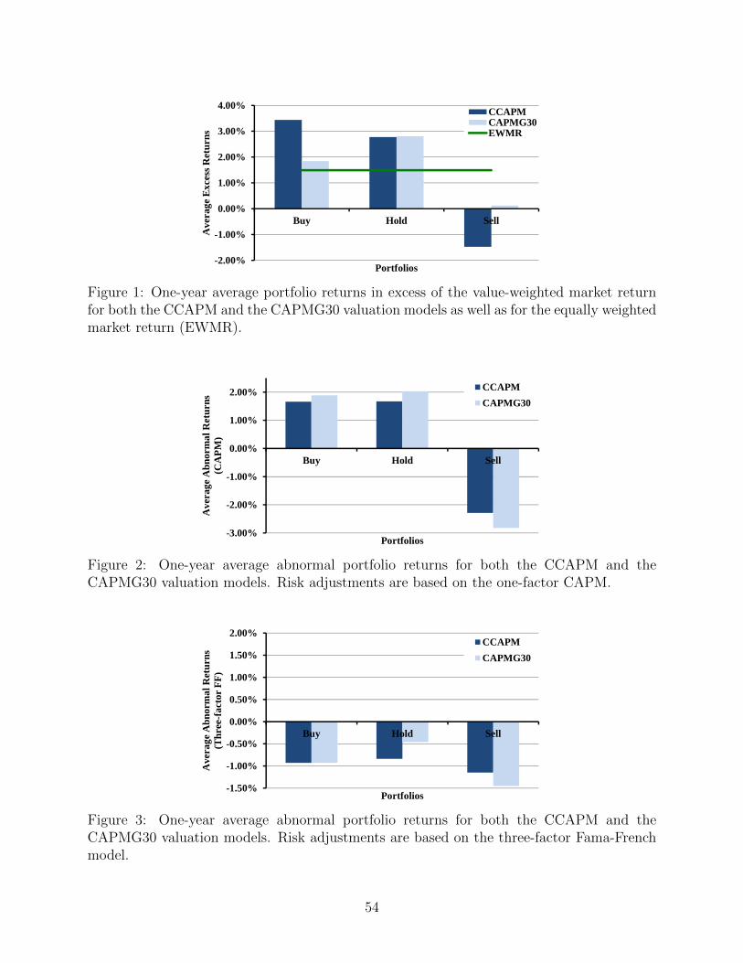
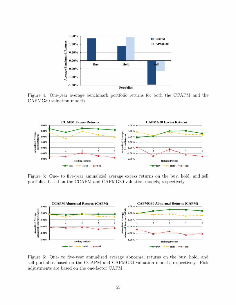
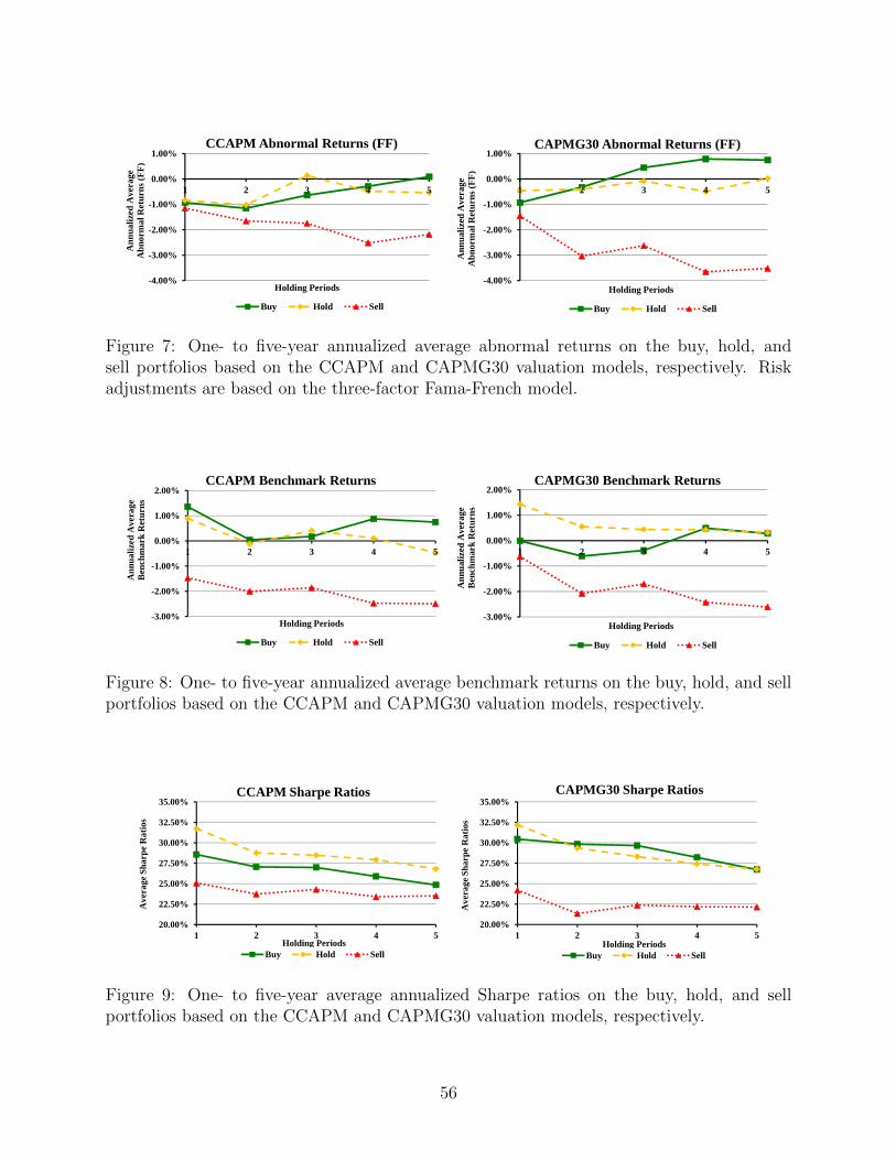
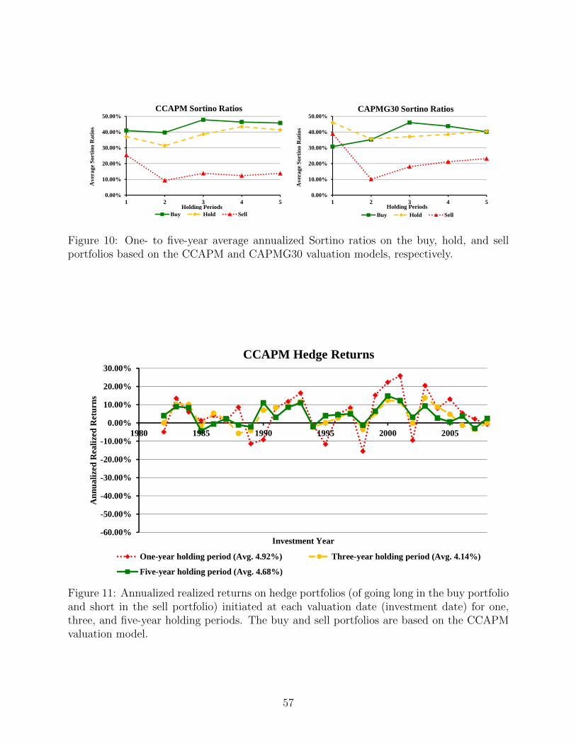
1These performance measures include excess returns relative to the value-weighted market index, ab-normal returns (i.e., with one-factor CAPM and three-factor Fama-French risk adjustments), benchmarkreturns based on firm characteristics, Sharpe, and Sortino ratios as well as the time-series of realized hedgereturns (long in buy portfolios and short in sell portfolios).

2See Frankel and Lee 1998 for a first study along these lines using the standard valuation model.

2

No one knows what the market premium is. And adopting multifactor pricing

models adds more risk premiums and betas to estimate. These models contain a

strong element of smoke and mirrors.”

Due to estimation errors, Levi and Welch (2014) show (using historical data and simulation

studies with known parameters) that users of the CAPM or the Fama-French model should

shrink the beta estimates (even on the industry level) almost to the point where there is no

cross-sectional variation in the cost of equity. Moreover, they report that, since 1970, the

geometric (arithmetic) equity premium relative to long-term Treasuries has been only 0.8%

(1.7%) annually.3 In their study, standard applications of both the CAPM and the Fama-

French model failed to predict rates of returns given estimated inputs, often even with the

wrong sign (see also Frazzini and Pedersen 2014). They argue it is much more important to

account for the easy-to-estimate term-premium on long- versus short-term Treasuries than

hard-to-estimate risk premiums in risk-adjusted expected rates of returns.

Using the standard series of aggregate consumption, the nominal price index from the

NIPA tables and a reasonable level of relative risk aversion (equal to two), the CCAPM-

based valuation model produces small estimated risk adjustments to forecasted residual

income (with a median NPV in the order of 2% of current book value). It is well known that

the stochastic variation in the aggregate consumption series is not sufficient to produce an

equity premium relative to short-term Treasuries around 6% for reasonable levels of relative

risk aversion (e.g., Mehra and Prescott 1985 and the extensive literature that followed on

the equity premium and risk-free rate puzzles). It is possible that too much averaging,

smoothing and estimation go into the constructing of this series, but it is worth noticing that

risk adjustments may be lower than suggested by this literature, once the term-premium is

properly accounted for by discounting risk-adjusted expected residual income with easy-to-

estimate zero-coupon interest rates. In any case, using the CCAPM-based valuation model,

the impact of difficult-to-estimate risk adjustments play a much smaller role in aggregating

residual earnings forecasts into a valuation than when standard valuation models are used.

While one- and two-year-ahead analyst forecasts are, in general, quite reasonable and in

accordance with subsequent accounting earnings, the reported growth rates for three- to five-

year-ahead forecasts seem to be substantially upwardly biased (e.g., Frankel and Lee 1998

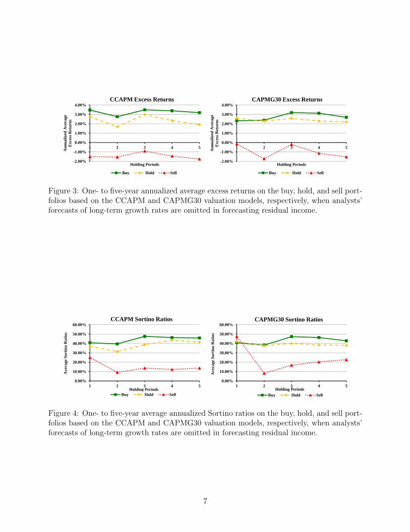
and Hermann et al. 2008). In a robustness check in the online appendix, we demonstrate that

excluding these long-term growth forecasts of analysts in our forecasting of future residual

income leads to significantly lower valuation accuracy, especially for the standard valuation

model. Hence, even though these long-term forecasts might be substantially upwardly biased,

3The standard procedure of using a 10-year Treasury rate plus a risk premium relative to a short-termTreasury rate may thus be double-counting for the term-premium leading to an overstated cost of equity.

3

they still seem to provide useful information for valuing stocks in the cross-section.

If the risk adjustments are upwardly biased (in the standard valuation models) or down-

ward biased (in the CCAPM-based valuation model) and the analysts’ growth forecasts are

upwardly biased, we can make a counterbalancing error in the growth rate in the continuing

values. We do this by calibrating the growth rates in the continuing values at each valuation

date to match the level of stock prices at that date (i.e., such that the median valuation

error is equal to zero). Of course, this requires that there be no systematic differences in the

biases in the cross-section of firms for each valuation model.

Using the standard valuation model, the medians of the calibrated growth rates in the

continuing value over the sample period are substantial, i.e., 5% (8%) when including (ex-

cluding) the analysts’ long-term forecasts in the analysis. Growth rates of expected future

value creation in the continuing value of that economically unreasonable magnitude suggest

that the standard valuation model must make a “counterbalancing error” of risk-adjusting

too much through the risk-adjusted cost of equity in the denominator.

Using the CCAPM-based valuation model, the medians of the calibrated growth rates in

the continuing value over the sample period are much lower, i.e., −10% (1%) when including

(excluding) the analysts’ long-term forecasts in the analysis. Hence, the continuing value

plays a much smaller role in valuations with the CCAPM-based valuation model. In this

model, risk-adjusted expected value creation is implied to “fade” to zero in the long-run (at

least when including analysts’ growth forecasts from three to five years ahead), consistent

with the economic theory of competition, real options to expand and abandon, and entry

and exit in product markets.4 On the other hand, the fading of risk-adjusted expected value

creation may also be a result of counterbalancing the upward bias in the analysts’ long-

term growth forecasts and downward biased risk adjustments due to the smooth aggregate

consumption series. Our analysis cannot separate these potential effects.

We implement several versions of the standard valuation model using an estimated cost

of equity as the discount rate for discounting expected future residual income and for calcu-

lating residual income as comprehensive income minus the cost of equity times the opening

book value of equity for the period. The implementations differ with respect to (a) growth

assumptions for residual income after using five-year-ahead analysts’ forecasts, (b) whether

we use a one-factor CAPM or a three-factor Fama-French model for estimating the cost

of equity, and (c) the historical period over which we estimate the factor risk premiums

at each valuation date. In general, we find that the valuation accuracy (measured primar-

ily as median absolute valuation errors) is better for long estimation periods of factor risk

4Note that this does not imply the accounting is unbiased—it only means that the expected unrecordedgoodwill has a limit equal to the risk adjustment for unrecorded goodwill.

4

premiums (30 years or more). The valuation accuracy is substantially better for the one-

factor CAPM than for the three-factor Fama-French model, and this result is consistent

with comparable results of Nekrasov and Shroff (2009). Hence, the additional risk factors in

the Fama-French model do not seem to offset the additional estimation noise and the lack

of stability in estimating more risk premiums even for long estimation periods (at least for

valuation purposes).

There is a large empirical literature comparing the valuation accuracy of mathematically

equivalent (given clean or super-clean surplus accounting) versions of the standard valua-

tion model such as discounted cash flow models and accounting-based models such as the

residual income model and the abnormal earnings growth model.5 The differences between

these equivalent models are a matter of how value is represented in the valuation equation.6

The empirically documented differences in valuation accuracy (usually favoring the residual

income model) of these versions of the standard valuation model are primarily due to the

length of the forecast horizon and how the continuing value is modeled after the forecast

horizon (e.g., Lundholm and O’Keefe 2001; Penman 2001; Jorgensen et al. 2011).

Our empirical comparison of the valuation accuracy and the investment performance

of the standard valuation models versus the CCAPM-based valuation model is different in

nature. We cast both types of models in the residual income valuation framework, but the

two model types differ fundamentally in how they adjust for risk in future residual income.

The standard valuation model is based on a single-period CAPM equilibrium framework,

which can only be meaningfully extended to a multi-period setting if the cost of capital

is constant and shocks to residual income are fully persistent on a percentage basis, i.e.,

residual income follows a geometric Brownian motion (which precludes residual income from

being negative in any future period).7 The CCAPM-based valuation model has its roots in

5In the discounted cash flow model, the value of equity is equal to the NPV of future cash flows to theequity holders. In the residual income model, the value of equity is equal to the current book value of equityplus the NPV of future residual income. In the abnormal earnings growth model, the value of equity is thecapitalized value of the sum of forward earnings and the one-year-ahead NPV of future abnormal earningsgrowth. All three types of models also come in versions on a net operating asset basis assuming that thefinancial activities are recorded on a mark-to-market basis in the reformulated financial statements (e.g.,Ohlson 1995; Feltham and Ohlson 1995; Feltham and Ohlson 1996; Feltham and Ohlson 1999; Christensenand Feltham 2003; Ohlson and Juettner-Nauroth 2005; Christensen and Feltham 2009; Penman 2007).

6The discounted cash flow model is nothing but a version of the accounting-based models assuming cashflow accounting. However, as has been the practice for several hundred years, financial statements havebeen on an accrual basis to recognize value creation on a more timely basis than cash flow accounting does.The appealing feature of accounting-based valuation models is that they recognize value creation on a moretimely basis (through accruals) with their principle of counterbalancing errors: any errors you may makein current accounting book values or earnings are precisely offset in the NPV of future residual income orabnormal earnings growth.

7See Section 5.4 in Christensen and Feltham (2009), and Brennan (2003) for the necessary and sufficientconstant relative risk condition for a constant return risk premium.

5

classical multi-period asset pricing theory (cf., Rubinstein 1976), and it allows for stochastic

interest rates, stochastic inflation, and time-varying risk adjustments to expected future

residual income depending on the time-series properties (such as mean reversion) of future

residual income.

Our study is closely related to that of Nekrasov and Shroff (2009). They perform an

empirical comparison of the valuation accuracy of standard valuation models and models

with fundamentals-based risk adjustments. While their valuation accuracy results for the

standard models are very similar to ours, their fundamentals-based risk adjustment model

is different. Their starting point is the same, namely that no-arbitrage and clean surplus

accounting imply that equity value can be written as the current book value of equity plus

the discounted value (with risk-free interest rates) of expected future residual income minus

a risk adjustment determined by the covariance between residual income and a valuation

index (see Feltham and Ohlson 1999). That is, they also discount for risk in the numerator

and discount for time with risk-free interest rates in the denominator. However, no-arbitrage

and clean surplus accounting alone do not inform about how the valuation index and, thus,

the risk adjustment is determined. The valuation index is a mathematical construct with no

economic content.

While no-arbitrage pricing is useful for pricing redundant assets, more structure is needed

to price primitive securities like equities. Nekrasov and Shroff (2009) follow the path in the

linear factor-based asset pricing literature (like the Fama-French model) making the ad hoc

assumption that the valuation index can be written as a linear function of some (accounting-

based) pricing factors like the Fama-French factors. Further assuming that the covariance

between residual income returns and the valuation index is constant across time (which

amounts to assuming no persistence in residual income returns) allows them to estimate

fundamentals- or accounting-based risk adjustments to expected future residual income.8

While there is no economic theory supporting the form of fundamentals-based risk ad-

justments by Nekrasov and Shroff (2009), they obtain substantial improvements in valuation

accuracy compared to both the standard one-factor CAPM and three-factor Fama-French

models using a risk-adjusted cost of equity. The improvements are of the same magnitude

as the improvements we obtain using the CCAPM-based valuation model.9 This suggests

that making the risk adjustments in the numerator rather than through a risk-adjusted cost

8Christensen and Feltham (2009) show in their Section 5.3 that mark-to-market accounting leads toresidual income returns with zero persistence. For other accounting policies, there is likely to be somepersistence in residual income returns if there is persistence in the underlying cash flows.

9Nekrasov and Shroff (2009) do not evaluate the different types of models from a fundamental valuationperspective. Rather, they find that their fundamentals-based risk measures can assist in understanding someof the standard “anomalies” such as the value premium.

6

of equity in the denominator is the key to improving valuation accuracy, and maybe not so

much whether the risk adjustments are based on an ad hoc factor model or they are based on

an equilibrium approach using, for example, the CCAPM. However, it is generally preferred

to have a well-founded economic theory behind empirical endeavors.

Our study and that of Nekrasov and Shroff (2009) compare alternative comprehensive

valuation models determining equity values in terms of current book value and net present

value of future residual income. The key difference is how the net present values of uncertain

future residual income are calculated. Another branch of the equity valuation literature

compares comprehensive valuation models to multiple-based equity valuation models in terms

of valuation accuracy (e.g., Liu, Nissim, and Thomas 2002). The latter models examine

which financial attributes (such as analysts’ one- and two-year-ahead earnings forecasts)

best explain market prices of comparable firms in a linear regression. The multiples are

determined at each valuation date so as to minimize the distance between market prices and

model values (i.e., the product of estimated multiples and financial attributes) in a given

industry of comparable firms. The key difference between the two types of models is that

the latter uses contemporaneous market prices of comparable firms to minimize the distance

between market prices and model values in the industry (such as the MAVE), whereas the

former does not use market prices of comparable firms but estimated discount rates, risk

adjustments, and growth rates in the continuing value.

Not surprisingly (given the research design), the multiple-based equity valuation models

perform better than comprehensive valuation models in terms of valuation accuracy. The

key result from the multiple-based equity valuation models is that simple models using

only analysts’ two-year-ahead earnings forecasts (and perhaps forecasted short-term earnings

growth) perform well. For example, using the sample period 1982–1999 and 81 industries

to estimate year- and industry-specific multiples, Liu, Nissim, and Thomas (2002) find a

MAVE of 16% using only the forecasted two-year-ahead price-earnings ratio.

Eliminating estimation noise and simplicity seem to be virtues in matching market prices

of equities. Multiple-based equity valuation models do not inform about the determinants of

fitted multiples and, thus, do not allow comparisons of equities across industries and time.

Hence, while multiple-based equity valuation models are useful to get a reading of what

the market price would be on a non-traded stock, these models are less useful as a tool to

challenge market prices of traded stocks based on fundamental analysis—unless it is assumed

all firms in the industry must have the same multiples, regardless of earnings persistence,

risk, growth, etc.; see Penman and Reggiani (2013).

The remainder of the article is organized as follows. Section 2 presents the standard

and CCAPM-based valuation models. Section 3 describes the data sources and the sam-

7

pling method. Section 4 describes the methods of implementing the valuation models. The

empirical results are presented in Section 5, and Section 6 concludes.

In the online appendix, we perform a few robustness checks concerning (a) the impact

of including financial companies and utilities in the empirical analysis and (b) the impact of

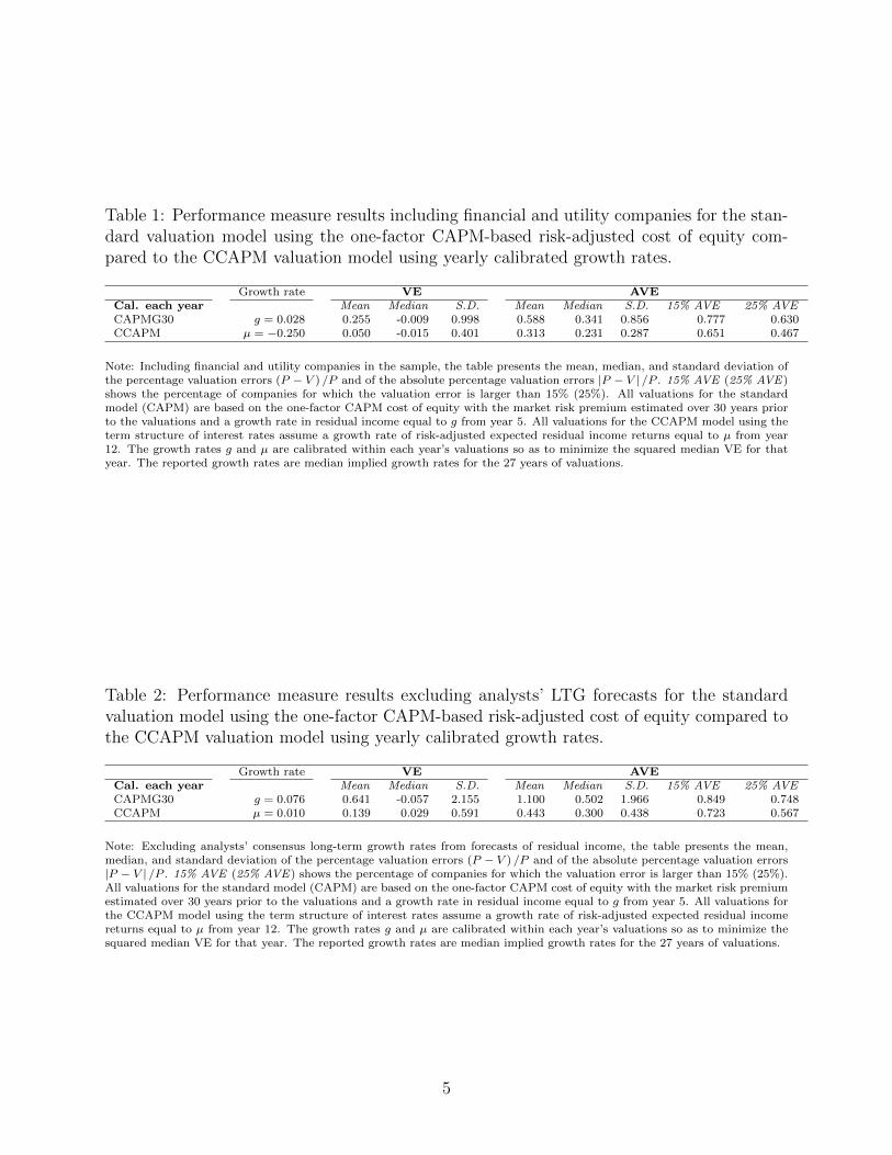
excluding the analysts’ long-term growth forecasts from the analysis. The key results are (a)

the relative empirical performance of the two model types is basically unchanged by including

financial companies and utilities, but the calibrated median growth rates in continuing values

are reduced (as should be expected based on the accounting principles used by these types

of firms), and (b) the valuation accuracy deteriorates by excluding the analysts’ long-term

growth forecasts and the median calibrated growth rates increase significantly for both model

types, but the empirical investment performance is almost as good as when these long-term

growth forecasts are included in the analysis.

2 Valuation models

In this section we present the standard and the CCAPM accounting-based valuation models,

and we show how they are based on classical asset pricing theory. The accounting structure

is similar in both types of models—they anchor the valuation in current book value and then

add a premium equal to the discounted forecasted residual income. The models differ in their

adjustment for risk. In the standard model, discounting for risk is done in the denominator

through a CAPM-based (or multi-factor) risk-adjusted discount factor. In the CCAPM-

based valuation model, forecasted residual income is adjusted for risk in the numerator,

and the risk-adjusted forecasted residual income is then discounted by the risk-free discount

factor. Hence, the latter disentangles the discounting for risk from the discounting for the

timing of forecasted residual income.

2.1 Fundamentals of asset pricing

Assuming no arbitrage and mild regularity conditions, a strictly positive state-price deflator

(SPD) m exists such that the price at date t, Vt, of any asset in the economy is given by

Vt =∞∑τ=1

Et [mt,t+τdt+τ ] ,

where d is the dividend from the asset, and Et[·] is the conditional expectations operator

given information at date t. The SPD discounts both for risk and timing of dividends. As

shown by Feltham and Ohlson (1999), an equivalent representation of the price separates

8

the adjustment for time from the adjustment for risk as

Vt =∞∑τ=1

Bt,t+τ {Et [dt+τ ] + Covt (dt+τ ,Qt,t+τ )} , (1)

where Bt,t+τ = (1 + ιt,t+τ )−τ = Et [mt,t+τ ] is the date t price of a zero-coupon bond paying

one dollar at date t+ τ , ιt,t+τ is the date t zero-coupon interest rate for maturity t+ τ , and

Qt,t+τ = mt,t+τBt,t+τ

is a valuation index.

An important criticism of the above dividend discount model (DDM) for valuation is that,

while a dividend payment in effect gives the investor a dollar amount, it is not necessarily

an indication of value creation by the firm (in the short term). A firm can borrow in order

to pay dividends, and Miller and Modigliani (1961) show that such a financing decision does

not create value: dividends are important to equity values but the dividend policy is not.

The residual income valuation (RIV) model reflects value creation in a more timely and

transparent form and is therefore often preferred in equity valuation. As shown by Feltham

and Ohlson (1999), the RIV model yields the same valuation as the DDM if the accounting

system satisfies the clean surplus relation (CSR):

bvt+τ = bvt+τ−1 + niτ − dτ , (2)

where bv is book value of equity, ni is net income, and d is the dividend (i.e., net transactions

with shareholders). That is, besides payments to shareholders, all changes in book value

of equity must be recorded in (comprehensive) net income. Defining residual income as

rit+τ = nit+τ − ιt+τ−1,t+τbvt+τ−1, Feltham and Ohlson (1999) show that no-arbitrage and

CSR imply that the DDM in (1) can be rewritten as the RIV model, i.e.,

Vt = bvt +∞∑τ=1

Bt,t+τ {Et [rit+τ ] + Covt (rit+τ ,Qt,t+τ )} . (3)

The various asset pricing models handle the risk adjustments, i.e., the conditional covariances

between future residual income and the valuation index, in different ways. In order to address

this, further assumptions are needed for identifying the valuation index.

2.2 Standard CAPM-based valuation model

The CAPM is a single-period theory, and it can be derived in several ways. One way

is to assume that the payoffs on the asset and the market portfolio are jointly normally

distributed, and that the valuation index can be written as a function of the payoff on the

9

market portfolio. Stein’s Lemma can then be applied to rewrite the single-period equivalent

of (1) as

Vt = Bt,t+1

{Et [dt+1 + Vt+1] + Et

[Q′t,t+1

(dMt+1 + V M

t+1

)]Covt

(dMt+1 + V M

t+1,dt+1 + Vt+1

)},

(4)

where dM + V M is the payoff on the market portfolio. Since this formula prices any asset

with normally distributed dividends and therefore also the market portfolio, it is straightfor-

ward to show (by substituting out Et

[Q′t,t+1

(dMt+1 + V M

t+1

)]from the formula for the market

portfolio) that the expected return of any asset is given by

Et [Rt+1] = ιt,t+1 +(Et

[RMt+1

]− ιt,t+1

) Covt(RMt+1,Rt+1

)Vart

(RMt+1

) = ιt,t+1 + rpt,t+1, (5)

where R is the return (= (dt+1 +Vt+1−Vt)/Vt) on the asset, RM is the return on the market

portfolio, and rp is the return risk premium, which is determined as the product of the asset’s

beta, i.e.,Cov(RM ,R)

Var(RM ), and the market risk premium, i.e., E

[RM]−ι. If an asset has low (high)

returns in periods in which the market returns are low, then the asset has a higher (lower)

required expected return than the riskless return, implying a lower (higher) asset value than

the expected payoff discounted at the risk-free rate. In the CAPM, the return on the market

portfolio is the only priced risk factor.

In our empirical study, we also consider the Fama-French multi-factor model. It can be

derived in a similar manner as the CAPM from an assumption that the valuation index can

be written as a linear function of priced risk factors. The return risk premium rp can in this

case be written as weighted sum of the factor risk premiums with the asset’s factor betas as

weights.

To calculate the expected return via (5), one has to estimate the asset beta and the

expected excess return on the market portfolio (see Section 4.1 below). To find the value

of the asset using the CAPM method, the risk-free rate, the beta, and the expected excess

return on the market portfolio must be assumed to be constants (see the discussion in

Christensen and Feltham 2009, Chapter 2). These are similar assumptions to those in

the CAPM valuation model implementations of Nekrasov and Shroff (2009) and Jorgensen

et al. (2011). With these assumptions, the standard valuation model can equivalently be

formulated as

Vt =∞∑τ=1

Et [dt+τ ]

(1 + ι+ rp)τ. (6)

This is the standard dividend discount model (DDM) stating that the value of an asset is

determined as its expected future dividends discounted by its risk-adjusted cost of capital.

10

Defining residual income as riSTDt+τ = nit+τ − (ι+ rp) bvt+τ−1 and using the clean surplus

relation (2 ), it is straightforward to rewrite (6) as the standard RIV model as

Vt = bvt +∞∑τ=1

Et

[riSTDt+τ

](1 + ι+ rp)τ

.

That is, the value of common shareholders’ equity is the sum of the book value of equity

and future expected residual income discounted by the risk-adjusted cost of equity. Dividing

through by the book value of equity at the valuation date allows us to write the market-

to-book ratio as the normal market-to-book ratio plus a book value premium equal to the

risk-adjusted discounted value of expected future Residual Income Returns, RIRSTDt,t+τ ≡

riSTDt+τ /bvt, i.e.,

Vtbvt

= 1 +∞∑τ=1

Et

[RIRSTD

t,t+τ

](1 + ι+ rp)τ

. (7)

The practical considerations involved in calculating the value of common shareholders’ equity

in a large-sample empirical study using (7 ) will be discussed and explained in Section 4.1.

2.3 CCAPM-based valuation model

As for the standard valuation model in (7), we base the CCAPM valuation model on the

clean surplus relation (2) and use residual income (RI). However, instead of discounting

expected future RI for both risk and time through a risk-adjusted discount rate in the

denominator (and a risk-adjusted capital charge in the definition of residual income), we first

make assumptions about the time-series properties of residual income returns and aggregate

consumption to obtain a closed-form expression for the risk adjustment in (3) directly. Hence,

forecasted future RIs are adjusted for risk in the numerator, and the risk-adjusted forecasted

future RIs are then discounted by zero-coupon interest rates.

The RIV model (3) prices all assets, but further assumptions are needed for the model

to be empirically implementable, since no-arbitrage and CSR only ensure the existence of

the valuation index but not what determines this index. One can proceed from (3) in

various ways. One possibility is to make an ad hoc assumption that the valuation index

is an affine function of some pricing factors and then use a standard factor-based model

approach like the Fama-French approach. This is the approach followed by Nekrasov and

Shroff (2009), and they use 10 years of historical accounting data to calculate a constant

risk-adjustment term using accounting-based Fama-French factors. Naturally, this places

strong assumptions on the data, such as many consecutive years of accounting data, and the

fact that a constant risk adjustment implicitly assumes no persistence and growth in residual

11

income (see below). Furthermore, there is no economic foundation of the model. We follow

the equilibrium approach by Christensen and Feltham (2009) and place assumptions on the

time-series properties of the variables in the model and from these time-series properties, we

obtain an explicit solution of the time-varying risk adjustment terms in (3).

We assume that a Pareto efficient equilibrium exists (as in the CAPM), that investors

have time-additive power utility, i.e., u (x) = 11−γx

1−γ, where γ is the common relative

risk aversion parameter and x is real consumption, and that real aggregate consumption

and the nominal price index are log-normally distributed. Let ci denote the consumption

index, which is a measure of real aggregate consumption and the nominal price level in the

economy.10 Under the additional assumption of future residual income and the consumption

index being jointly normally distributed, Christensen and Feltham (2009) show that (3) can

be reformulated as

Vtbvt

= 1 +∞∑τ=1

Bt,t+τ [Et (RIRt,t+τ )− Covt (RIRt,t+τ ,cit+τ )] , (8)

where RIRt,t+τ ≡ rit+τbvt

, rit+τ = nit+τ − ιt+τ−1,t+τbvt+τ−1, cit+τ = ciRt+τ + ln (pt+τ ) =

γ ln (ct+τ ) + ln (pt+τ ) and c is aggregate consumption per capita, whereas p is a nominal

price index. The consumption index can be estimated from observed data and an assump-

tion about γ as will be discussed in Section 4.2.

Following Christensen and Feltham (2009), we assume a simple first-order autoregressive

model for RIR given by11

RIRt,t+τ −RIRot = ωr [RIRt,t+τ−1 −RIRo

t ] + εt+τ , (9)

where RIRot is the structural level of the residual income return at the valuation date t, |ωr| <

1 is the first-order autoregressive parameter determining the speed of convergence to the

structural level of residual income return, and ε are i.i.d. normally distributed innovations.

The motivation behind assuming an autoregressive process with mean reversion towards a

structural level is inspired by, for example, Penman (2007), who argues that, in practice, the

strong force of competition (and entry and exit) is often assumed to drive residual income

towards a structural level, such as an industry average.

10With our assumption of standard power utility, the consumption index is the product of relative riskaversion and log aggregate consumption per capita plus the log of the price index (see Christensen andFeltham 2009).

11For simplicity, we consider a simplified version (compared to Christensen and Feltham 2009) of theprocess for residual income returns in which there is no growth in the structural level of residual incomereturns. Allowing for growth does not yield substantially improved empirical results.

12

We assume that the consumption index ci follows the simple process

cit+τ − cit+τ−1 = υ + δt+τ , (10)

which is consistent with the standard asset pricing assumption of aggregate consumption

being log-normally distributed (i.e., aggregate consumption per capital follows a geometric

Brownian motion). The assumption of a constant growth rate υ further implies constant

interest rates (see Christensen and Feltham 2009, Chapter 5). The innovations in the above

equations, ε and δ, are assumed to be serially uncorrelated and to be distributed as[εt+τ

δt+τ

]∼ N

(0,

{σ2r σra

σra σ2a

}).

That is, ε and δ are contemporaneously correlated, which reflects the systematic risk in

residual income returns.

Solving equations (9) and (10) recursively yields

RIRt,t+τ = RIRot + ωτr (RIRt,t −RIRo

t ) +τ−1∑s=0

ωsrεt+τ−s, (11)

cit+τ = cit + τυ +τ−1∑s=0

δt+τ−s. (12)

From the residual income return equation (11), it follows that

Et [RIRt,t+τ ] = RIRot + ωτr (RIRt,t −RIRo

t ) ,

Vart [RIRt,t+τ ] = σ2r

1− ω2τr

1− ω2r

.

From the consumption index equation (12), it similarly follows that

Et [cit+τ ] = cit + τυ, Vart [cit+τ ] = τσ2a.

Furthermore, the covariance between the two series is given by

Covt (RIRt,t+τ ,cit+τ ) = σra1− ωτr1− ωr

. (13)

The risk adjustment to the expected residual income return is determined by the covariance

between the residual income return RIR and the consumption index ci. The higher the

13

covariance, the larger is the adjustment for risk, since the asset provides a less valuable hedge

against periods with low consumption. The risk adjustment depends on the contemporaneous

covariance between the innovations in residual income returns and the consumption index

σra and on the persistence of deviations of residual income returns from their structural level

ωr. For σra > 0, the risk adjustment is increasing in the persistence parameter ωr. That

is, the slower is the reversion of residual income returns to the long-run structural level, the

higher is the risk adjustment. This is an intuitive result, since future residual income returns

are more uncertain, the lower is the degree of mean reversion. The covariance between

RIR and ci (i.e., the risk adjustment) is converging towards an upper limit of σra/ (1− ωr).In the simple case of instant mean reversion (i.e., zero persistence), i.e., ωr = 0, the risk

adjustment to the expected residual income returns is constant (as in the Nekrasov and

Shroff 2009 model), i.e., Covt (RIRt,t+τ ,cit+τ ) = σra.

A major criticism of the standard model is that it discounts expected future residual

income by a constant risk-adjusted cost of equity. Ang and Liu (2004) emphasize that this

is not a reasonable assumption, and using a calibrated version of their model, they show

that economically significant valuation errors can be induced. Christensen and Feltham

(2009) show that the implicit risk adjustments to expected residual income returns from

using a constant return risk premium grows exponentially over time, and that this growth

is amplified by growth in the expected residual income returns. This is consistent with

the fundamental RIV model (3) when residual income returns follow a geometric Brownian

motion with zero mean reversion. On the other hand, the CCAPM valuation model has

time-varying adjustments for risk determined by the persistence of deviations of residual

income returns from their structural level, for example, due the sustainability of competitive

advantages.

Further assumptions are needed for the model to be empirically implementable in a

large-sample empirical study. These will be described in Section 4.2.

3 Data and sample

Having set the theoretical framework for the two types of valuation models, this section

describes the data needed for the empirical valuation study using the standard CAPM-

based valuation model (in Section 2.2) and the CCAPM-based valuation model (in Section

2.3).

We perform valuations at the end of April each year from 1982 until 2008. We use

analysts’ one- and two-year consensus forecasts from the month of April available through

the I/B/E/S database. Applying analysts’ forecasts of the long-term growth (LTG) rate to

14

the two-year forecast, we calculate three- to five-year-ahead earnings forecasts. The I/B/E/S

database contains April earnings per share (EPS) forecasts for 16,918 US companies (see

Table 1). By applying forecasts from the month of April, all companies with financial years

following the calendar year are expected to have made their annual financial report public

at the time of the forecast. This mitigates information asymmetry between investors at

the valuation dates. Furthermore, analysts often update their earnings forecasts after the

release of an annual report in order to reflect their updated information. Thus, April earnings

forecasts are expected to be relatively more updated than earnings forecasts in other months

of the year. The financial year of most companies follows the calendar year, and we only

keep these companies in the sample. Table 1 shows the impact of sampling on the number

of distinct tickers/companies available in the analysis.

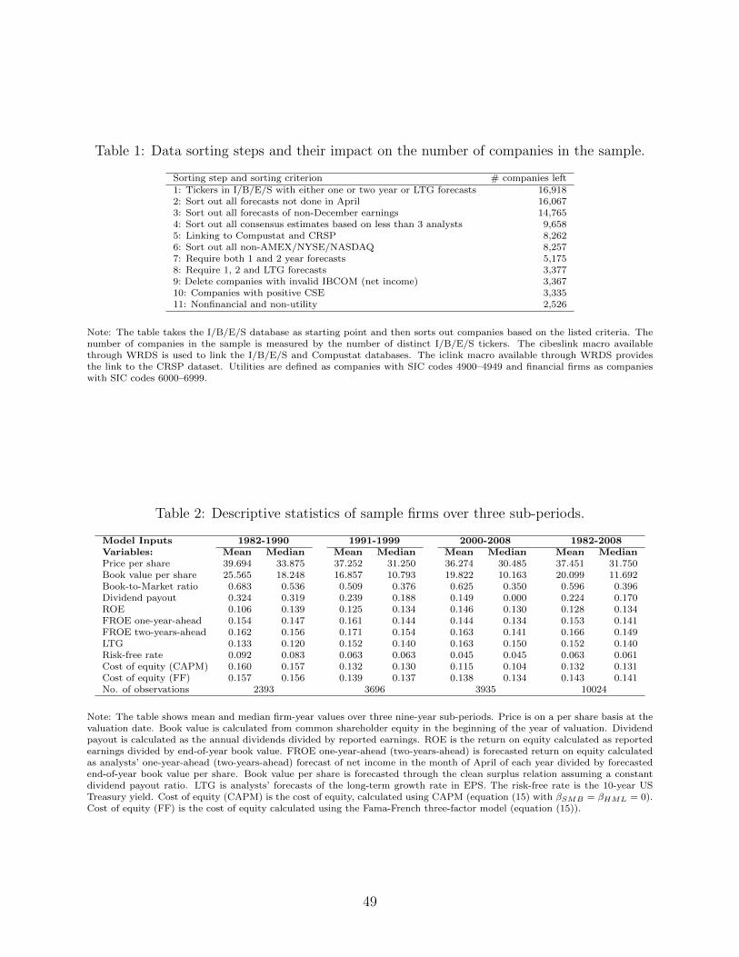
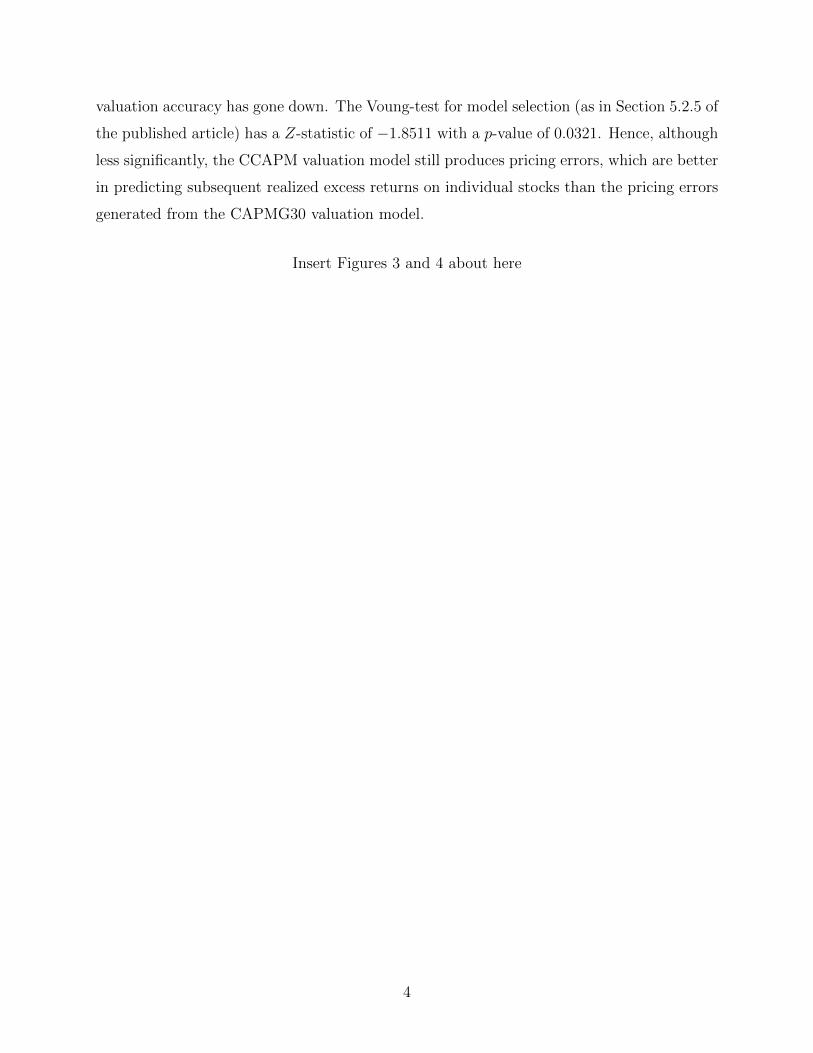
Insert Table 1 about here

In order to ensure a sufficient quality of the consensus EPS forecasts, we exclude median

forecasts based on less than three analysts. This approach is not standard in the literature,

and it reduces the number of distinct companies in the sample to 9,658 (see Table 1), which

is a relatively large reduction in the sample size. However, requiring at least three April

analysts’ forecasts for both one- and two-year-ahead forecasts and long-term growth-rate

forecasts mitigates the size effect on returns of small versus large firms documented in prior

literature (ensuring that we only retain relatively large firms with a high degree of analyst

following in the sample).

In addition to the I/B/E/S database, we use accounting information from the Compustat

database and stock price information from the CRSP database. The three databases use

different unique tickers for the companies, and none of these provide the link to the tickers

used in the other databases. A link between these databases is constructed based on the

cibeslink macro to link I/B/E/S to Compustat and the iclink macro to link I/B/E/S to

CRSP.12,13 Since the links between databases are imperfect and there are differences in the

variety of companies in the different databases, the sample size is reduced to 8,262 companies

(see Table 1). Most companies in the data set are traded on the major stock exchanges

(AMEX, NYSE, and NASDAQ). We exclude companies not traded on these exchanges.

As will be shown later, the standard CAPM-based valuation model is highly dependent

12These macros are available through WRDS. To link the databases to each other, we use the IDUSMdata set from I/B/E/S and the STOCKNAMES data set from CRSP.

13The linking quality between I/B/E/S and CRSP is based on a score from 0 to 6, where 0 is the bestmatch. We do not accept scores above 1, which should ensure that we only keep correctly matched firms. Asmall fraction of the I/B/E/S tickers have multiple links to CRSP tickers. In these cases, we only keep thecompany if it has a linking score of 0 and the score is unique.

15

on the estimates of LTG. Therefore, we need both one- and two-year-ahead earnings forecasts

as well as the LTG rate at the time of the valuation. If one of these forecasts is unavailable

at a valuation date, we exclude that observation from the sample. As is seen from Table 1,

this reduces the sample dramatically to 3,377 companies, yielding 20,499 distinct firm-year

observations.

As in Fama and French (2001), we exclude utilities (SIC codes 4900–4949) and financial

firms (SIC codes 6000-6999), limiting the analysis to 14,220 firm valuation dates and 2,526

distinct firm tickers spanning the period from 1982 to 2008.

The end-of-year book value of common equity (CSE) (Compustat item #60), net income

before extraordinary items (net income/IBCOM) (Compustat item #237), dividends paid

to common equity (Compustat item #21), and total assets (Compustat item #6) are from

Compustat. The stock price (CRSP variable PRC) and shares outstanding (CRSP variable

SHROUT) are from CRSP. Betas for each company in each valuation year are estimated

using monthly excess stock returns (CRSP) and monthly excess returns on the three Fama-

French factors (from the Fama-French database). The method is briefly described in Section

4.1. Following Nekrasov and Shroff (2009), we use a 60 month sample for each estimation

whenever such data is available from CRSP. If 60 months of data is not available, we allow for

a minimum of 36 months. The betas are estimated using 60 observations for most estimations

(10,752); 1,384 estimations are based on less than 60 but at least 36 observations, while

2,084 estimations were excluded from the valuation due to lack of data. Following the same

approach, betas are also calculated using the Fama-French three-factor approach. After

the estimations of betas, the sample size is limited to 12,136 valuations on 1,938 distinct

companies.

For the estimation of betas, we use the one-month Treasury rate as the risk-free rate.

In the standard CAPM-based valuation model we use, as is standard in both practice and

in the literature, a 10-year Treasury rate for calculating the risk-adjusted cost of equity

used for discounting and calculating expected future residual income. In the CCAPM-based

valuation model, we use zero-coupon interest rates from the FED database for discounting

risk-adjusted expected future residual income and the corresponding one-year-ahead forward

rates for calculating expected future residual income. In order to examine the impact of using

the yield curve in the CCAPM-based valuation model, we also implement this model with a

constant risk-free rate equal to the 10-year Treasury rate.

A number of observations are deleted during the valuation process using the CCAPM-

based valuation model, as will be described in Section 4.2. Thus, the results reported in

the results section are calculated using 10,024 valuations on 1,827 distinct companies. This

is fewer valuations compared to valuation articles such as those of Nekrasov and Shroff

16

(2009) and Jorgensen et al. (2011). There are several reasons for this. (a) we include only

nonfinancial and non-utility in the sample; (b) we require each valuation to have both a

one-year and two-year-ahead forecast as well as a forecast of LTG; (c) we do not include

consensus forecasts based on less than three analysts’ forecast; (d) unlike Jorgensen et al.

(2011), we require 36 observations in the estimation of betas; (e) additional sampling must

be done to apply two distinct valuation models and not just the standard valuation model

as used by Jorgensen et al. (2011). The Points (a)–(c) each reduce the sample significantly,

as seen from Table 1, while point (d) also has some impact. As a robustness check, we also

perform the analysis relaxing the criterion in point (a), and we show that the inclusion of

utilities and financial firms has no impact on the basic conclusions from the analysis. Further

robustness checks show that the CCAPM-based valuation model fares well both with and

without the LTG rate of analysts (see the online appendix).

In order to implement the CCAPM-based valuation model, we need data on real con-

sumption per capita as well as on the price index. The consumption data is the usual series

used in the CCAPM asset pricing literature. It is obtained from the NIPA tables available

from Bureau of Economic Analysis. The price index is also available from the NIPA tables.

Details on calculation of the consumption index will be given in Section 4.2.

4 Valuation procedure

This section describes how the valuation models are implemented in our large-sample em-

pirical study. Both models require a number of assumptions to be made in the empirical

implementation, and the empirical results depend on these assumptions. As a consequence,

we will perform the valuation based on several different assumptions, for example, about the

growth rate in the continuing value and about the factor risk-premium estimation. While the

standard model places stronger requirements on data availability, the implementation issues

are well explained in the literature and, therefore, we only briefly explain how we implement

this model. We will be more detailed in describing how we implement the CCAPM model.

4.1 Standard model procedure

The standard valuation model cast in the residual income framework is equation (7):

Vtbvt

= 1 +∞∑τ=1

Et

[RIRSTD

t,t+τ

](1 + ι+ rp)τ

. (14)

17

While the valuation equation may appear very simple, it is debated in the literature how best

to implement it. The model requires forecasting of future residual income and estimation of

the risk-adjusted discount factor taking account of discounting for both time and risk. The

model, as stated in (14), includes an infinite sum. Since forecasting into the infinite future is

not feasible, a truncation point is usually chosen, and a continuing value is calculated using

simplifying assumptions to account for the remaining. We discuss these elements in turn.

4.1.1 Discounting for time and risk

In the valuation equation (14), discounting for time and risk is done using a risk-adjusted

discount rate reflecting the risk associated with the payoffs to the equityholders, i.e., by the

cost of equity determined as the risk-free interest rate plus a return risk premium, ι+ rp. As

is standard in most valuation studies, we chose the risk-free rate to be the 10-year Treasury

yield (to reflect an average interest rate over the yield curve), and we allow for several priced

risk factors. Hence, the cost of equity is expressed as

ι+ rp = ι10y + β ·RP,

where ι10y is the 10-year Treasury yield, β is a vector of factor sensitivities, and RP is a

vector of factor risk premiums. We estimate the betas at each valuation date for each firm

using up to 60 observations of monthly data in the regression:

R− ι1m = a+ βMKTExRM + βSMBRSMB + βHMLR

HML + ε, (15)

where ι1m is the one-month Treasury yield, R is the return on the asset of interest, ExRM

is the excess return on the market portfolio, RSMB is the return on the Fama-French small

minus big portfolio, and RHML is the return on the Fama-French high minus low portfolio.

We run this regression both including only the market factor (i.e., the standard CAPM

assuming βSMB = βHML = 0) and including all three Fama-French factors.

The estimated betas are used to calculate the cost of equity as (when using all three

factors):

ι+ rp = ι10y + βMKTRPM + βSMBRP

SMB + βHMLRPHML,

where RPM , RP SMB, and RPHML are the historical risk premiums on the market, small

minus big, and high minus low portfolios, respectively.14 We estimate RPM , RP SMB, and

RPHML as the geometric average of (excess) returns over the rolling windows of 5, 10, 20,

and 30 years preceding the estimation date as well as the full period from 1926 until the

14The cost of equity is estimated using monthly data and is then annualized.

18

month preceding the estimation date. Hence, we obtain 10 different measures for the cost

of equity for each firm at each valuation date (i.e., standard CAPM versus Fama-French

models and five different rolling windows for the estimation of the factor risk premiums in

both models). In very rare cases, the cost of equity is below 2%, and we winsorize it to

2%. This winsorization has effect more often in the three-factor than in the one-factor case,

and more so using few observations in the estimation of risk premiums than when many

observations are used.

4.1.2 Forecasting book value of equity and residual income

The standard valuation model in (14) requires forecasts of residual income riCAPMt+τ = nit+τ−(ι+ rp) bvt+τ−1, which means that we must make forecasts of future net income and book

values of equity. In order to obtain these forecasts, we use the most recent book value

of equity, which is calculated from accounting data from the Compustat database for the

previous year. Following Nissim and Penman (2001), we calculate common shareholders’

equity as

Common shareholder equity (CSE) = Common equity (#60) (16)

+ Preferred treasury stock (#227) - Preferred dividends in areas (#242).

To forecast residual income, we use analysts’ estimates of five-year-ahead forecasts of net

income ni from the I/B/E/S. Residual income for the first forecast year can then be calcu-

lated directly from the residual income formula rit+1 = nit+1 − (ι+ rp) bvt. Since the book

value of equity is unknown at future dates, we follow the standard procedure in the literature

(e.g., Frankel and Lee 1998; Claus and Thomas 2001; Gebhardt et al. 2001; Easton 2002)

and forecast this value through the CSR (2) by assuming a constant payout ratio equal to

the current payout ratio, which is calculated as

Dividends Common/Ordinary (#21)

Income Before Extraordinary Items (#237). (17)

If the firm has negative net income (#237), we calculate the payout ratio by dividing current

dividends with 6% of total assets (#6), i.e., the historical payout ratio. If the current payout

ratio is above 100%, we first calculate it by dividing current dividends with 6% of total

assets. If this also yields a payout ratio larger than 100%, we winsorize at 100% to ensure

that the company does not liquidate itself.

Having a starting value for book value of equity, forecasts of net income, and a constant

payout ratio, one can forecast future book values of equity through the CSR (2). With the

19

forecasted book value of equity, forecasted net income, and a constant cost of equity, we

forecast residual income five years ahead.

4.1.3 Continuing value

The final element in the valuation equation (14) is the infinite sum. We truncate 12 years

ahead and let residual income evolve according to a Gordon growth formula thereafter. We

follow Jorgensen et al. (2011) and implement several assumptions for the continuing values

in the standard valuation model to accommodate suggestions made in the literature as how

to calculate continuing values. The general formula we apply is given by

Vtbvt

= 1 +5∑

τ=1

Et

[RIRSTD

t,t+τ

](1 + ι+ rp)τ

+12∑τ=6

Et

[RIRSTD

t,t+τ

](1 + ι+ rp)τ

+Et

[RIRSTD

t,t+12

](1 + g)

(1 + ι+ rp)12 (ι10y + rp− g),

where g is the constant growth rate in residual income after year 12. The third part of the

above formula forecasts and discounts residual income from 6 to 12 years ahead. We assume

an intermediate convergence period from 6 to 12 years ahead, where we let residual income

converge to a certain level as described below. Twelve years ahead, we calculate a continuing

value based on residual income in year 12 and constant growth in residual income thereafter.

The first approach is a no growth case (CAPMC), in which we assume residual income

remains constant after the explicit forecast period if Et[riSTDt+5 ] > 0 and assume g = 0

in the continuing value. If Et[riSTDt+5 ] < 0, we let residual income revert towards zero in the

intermediate period and assume g = 0 in the continuing value. The second approach assumes

residual income grows 3% in both the intermediate period and the continuing term (CAPMG)

if Et[riSTDt+5 ] > 0, and otherwise we let it revert to zero. The third approach assumes the

return on equity Et

[nibv

]reverts to the historical industry average in the intermediate period

and that residual income remains constant after 12 years (CAPMI). The industry definitions

follow the Fama and French (1997) 48-industry classification. In the CAPMI approach, we

forecast residual income based on a growth rate calculated such that the return on equity

equals the historical average industry return on equity at year t+ 12. If the return on equity

is nonpositive at the valuation date, a feasible growth rate cannot be calculated for the firm

of interest and, thus, we let the return on equity revert linearly to the historical industry

return on equity.

20

4.2 CCAPM model procedure

There are several approaches to implementing the CCAPM valuation model in equation (8):

Vtbvt

= 1 +∞∑τ=1

Bt,t+τ (Et (RIRt,t+τ )− Covt (RIRt,t+τ ,cit+τ )) . (18)

Christensen and Feltham (2009) discuss using the information contained in the term structure

of interest rates to derive the implied preference dependent parameters of the model, such as

the relative risk aversion parameter γ, which is contained in the consumption index. While

this is a valid and appealing approach, we have chosen to implement the simpler approach

of assuming a particular relative risk aversion parameter γ = 2, which is a commonly used

value for γ in the asset pricing literature (e.g., Campbell and Cochrane 1999; Wachter 2006).

Fortunately, untabulated results show that the sensitivity of our empirical results is low with

respect to this parameter (within what is normally considered to be reasonable bounds from

one to ten). This is in stark contrast to the well-documented high sensitivity of valuations in

standard valuation models with respect to the market risk premium (or factor risk premiums).

No one knows the market risk premium and the investors’ relative risk aversion, and both

quantities are likely to vary over the business cycle (see Cochrane 2005a). It is an empirical

question which approach works best, but we leave it for future research.

Having specified the relative risk aversion parameter, we can use historical aggregate

consumption and price level data to estimate the time-series properties of the consumption

index, and we can use historical accounting data to estimate the time-series properties of

residual income returns. Our implementation of the CCAPM valuation model follows an

eight step procedure outlined below. (See the appendix for an application of this procedure

for valuing a specific company, Alcoa Inc., at a specific valuation date, April 15, 2002.)

(a) We use zero-coupon interest rates from the FED database to calculate the risk-free

discount factors Bt,t+τ , and we use the implied forward rates as estimates of future

spot interest rates in the calculation of future residual income returns.15 In order to

examine the impact of using a non-flat yield curve, we also consider a variation of the

model in which the 10-year Treasury yield is used as a constant risk-free discount rate

and as the risk-free spot rate in the calculation of future residual income returns.

15This is consistent with our process for the consumption index, which as noted implies deterministicinterest rates. For more general consumption index processes with, for example, mean reversion, interestrates become stochastic and, therefore, there is an additional risk-adjustment term in the accounting-basedresidual income model using forward rates in the calculation of residual income (see Christensen and Feltham2009, Chapter 3).

21

(b) Net income and book value of equity are forecasted one to five years ahead using ana-

lysts’ forecasts and an assumption of a constant payout ratio as in the standard model.

Using the interest rate assumptions from step (a) allows us to construct forecasts of fu-

ture residual income returns. An alternative would be to use the estimated time-series

model of residual income returns (from step (d) below) to forecast future returns, but

we have chosen to use analysts forecasts, because these forecasts are based on a much

richer information set than just past residual income returns.

(c) As in the standard model, we use an intermediate period of forecasts from year six to

year 12. For simplicity, we assume that residual income returns remain constant in the

intermediate period if Et[RIRt,t+5] > 0 and increase to zero if Et[RIRt,t+5] < 0.

(d) The risk adjustments in (13) require an estimate of the persistence of residual income

returns in the time-series model of these returns in (9) and an estimate of the contem-

poraneous covariance between the innovations in (9) and (10). We assume that the

sustainability of competitive advantages and the accounting principles used are similar

for all firms within an industry and, thus, we estimate the structural level of residual

income returns RIRot and the persistence of residual income returns ωr at the industry

level (for which we again use the Fama and French 1997 48-industry classification).

At each valuation date, we estimate the first-order autoregressive equation (omitting

cross-section subscripts)16

RIRt,t+τ = RIRot + ωr (RIRt,t+τ−1 −RIRo

t ) + εt+τ , τ = −7,− 6,...,0,

where the LHS is a time series of RIR from seven years before the valuation date (using

the book value of equity at the valuation date for each firm in the calculation of firm-

specific historical residual income returns). The industry-specific parameters RIRot and

ωr are estimated using a simple panel data model for each industry at each valuation

date.17 We take the average of the firms’ estimated error terms at each date in the

panel data estimation as the estimate of the industry-specific innovation at that date.

This provides a time-series of estimated industry-specific innovations, which, in step

(f) below, can be used to estimate the industry-specific contemporaneous covariance

between residual income returns and the consumption index.

16Consistent with the definition of residual income in the CCAPM valuation model, we use historicalone-year Treasury yields in the calculation of historical residual income returns.

17Convergence of the estimation could not be reached in a few cases, and in few cases the estimatedpersistence was larger than one, i.e., |ωr| ≥ 1. These cases are deleted from the sample.

22

(e) The consumption index is calculated from historical data from the NIPA tables as

cit+τ = γ ln (ct+τ ) + ln (pt+τ ) ,

where c =(cN

pN+ cS

pS

)/I, with N and S denoting nondurable and services, respectively,

and I is the population size. The weighted price index is calculated as p = cN

cN+cSpN +

cS

cS+cNpS. Consistent with the asset pricing literature, we assume as noted above that

the constant relative risk aversion is equal to 2, i.e., γ = 2. We assume constant growth

in the consumption index, and we use seven years of data to estimate the consumption

index equation (10):

cit+τ − cit+τ−1 = υ + δt+τ , τ = −7,− 6,...,0.

This yields a time series of estimated innovations δ in the consumption index at each

valuation date.

(f) With the results from steps (d) and (e), we estimate the contemporaneous covari-

ance between residual income returns and the consumption index, σra, as the simple

historical covariance between the time series of estimated innovations ε and δ. The

industry-specific risk adjustments to expected future residual income returns at each

valuation date are then calculated using the equation for the risk adjustment (13):

Covt (RIRt,t+τ ,cit+τ ) = σra1− ωτr1− ωr

. (19)

We use this risk adjustment to forecasted residual income returns for years until the

truncation year t+12. The parameters of the risk adjustment are constant and must be

known at the valuation date. The persistence ωr is estimated in step (d) as an industry-

and valuation-year specific parameter. While σra is constant for each valuation date,

the covariances in (19) determining the risk adjustments to future expected residual

income returns will be time varying.

(g) As for the standard valuation model, we truncate the model at year t + 12 and use a

Gordon growth formula for the continuing value. We assume the risk-adjusted expected

future residual income returns grow at a constant rate µ after year t+12, and we use the

longest zero-coupon interest rate in the FED database for discounting all risk-adjusted

expected future residual income returns after year t+12, denoted ιt,∞. The continuing

value is discounted by the 12-year zero-coupon interest rate. In the empirical study,

we use several assumptions for the growth parameter µ to provide fair comparisons to

23

the best implementation of the standard valuation model (see Section 5.1).

(h) Finally, the value of the common shareholders equity is calculated by adding the ele-

ments of the previous steps in the valuation equation (18):

Vtbvt

= 1 +5∑

τ=1

Et (RIRt,t+τ )− σra 1−ωτr1−ωr

(1 + ιt,t+τ )τ+

12∑τ=6

Et (RIRt,t+τ )− σra 1−ωτr1−ωr

(1 + ιt,t+τ )τ

+

[Et (RIRt,t+12)− σra 1−ω12

r

1−ωr

](1 + µ)

(1 + ιt,t+12)12 (ιt,∞ − µ),

where the third term on the RHS depends on whether Et (RIRt,t+5) is positive or

negative (see step (c)). If an equity value is estimated to be negative, it is deleted from

the sample.

5 Empirical results

To evaluate the empirical performance of the CCAPM- and the standard CAPM-based

valuation models, we compare the two model types along two dimensions. First, we compare

the models’ ability to match the cross-section of stock prices as well as the level of stock

prices across business cycles. This is the market efficiency perspective, which assumes that

the market prices of stocks are always right. Any comprehensive valuation model makes

assumptions about, for example, growth, risk, and how risk is priced, and is thus merely

a model of reality. If a particular valuation model provides a relatively good match to

market prices, the model may also provide better guidance compared to other models when

there is no observable market price, for example, when determining the offering price of

privately held companies for their initial public offerings, when determining equity values

in management buyouts and takeovers, and even in the evaluation of strategies and capital

budgeting decisions within firms. We follow the literature (such as Nekrasov and Shroff

2009) and examine the performance of the two model types along this dimension in Section

5.1 using the median absolute valuation error (MAVE) as our primary performance measure.

We then examine the ability of the two model types to identify cheap and expensive

stocks. This is the fundamental valuation perspective (e.g., Penman 2007), which assumes

that market prices of stocks may deviate from their fundamental values temporarily, but

that market prices will eventually revert to their fundamental values as determined by the

valuation model. If a valuation model can identify cheap and expensive stocks, then this

must be reflected in excess returns on trading strategies buying cheap stocks and selling

expensive stocks. We examine the performance of the two model types along this dimension

24

in Section 5.2 using excess returns on simple buy-and-hold strategies as our primary perfor-

mance measure. We use both short- and longer-term holding periods (one to five years) to

account for the fact that it may take time and market pricing errors might even get larger

before mispriced stocks eventually revert to their fundamental values.

5.1 Comparing model values with market prices

Table 2 reports descriptive statistics of key variables used as input to the valuation models.

The data set is split into three nine-year sub-periods, and both mean and median measures

are reported. Both the mean and median price per share are decreasing through the sampling

period, and this pattern is opposite to what is observed by Nekrasov and Shroff (2009). One

explanation of this difference is that Nekrasov and Shroff (2009) require each company to

have 10 consecutive yearly observations of accounting data, and this can introduce a strong

survivorship bias in their dataset. This explanation is supported by the dividend payouts,

which are showing the same decreasing pattern as documented by Nekrasov and Shroff (2009)

but are smaller, compared to their reported values. All other variables show largely the same

patterns and values shown by Nekrasov and Shroff (2009). The book value per share and the

book-to-market ratio have decreased since the 1980s, reflecting the bull market over most of

the two later sub-periods. The mean (median) dividend payout has been decreasing steadily

through the period from a high of 32.4% (31.9%) in the earliest sub-period to 14.9% (0%) in

the latest sub-period. Since these payout ratios only include dividends in the classical sense

and not other types of distributions to shareholders, it is likely that much of this decrease

can be explained by the documented increase in share repurchases.18

The mean return on equity is increasing through the sample period, while the median is

largely unchanged.19,20 This pattern is matched relatively well by analysts’ forecasts of return

on equity for the subsequent one and two years. The long-term growth rate is increasing

slightly for both the mean and the median values through the sampling period. Analysts, in

general, seem to be biased towards reporting too high growth rates. Average growth rates

well in excess of 10 percent predicted for all sub-periods cannot be realized in reality over

substantial periods. While analysts’ expectations about the short term are reasonably accu-

rate (or moderately upwardly biased), forecasts of long-term growth are strongly upwardly

18A relative increase in share repurchases is documented by Dittmar (2000) for the period 1977–1996 andby Fama and French (2001) for the period 1978–1999.

19Beginning-of-year book value is not available for all companies since it requires accounting data from ayear before the valuation date. Therefore, ROE is reported using end-of-year book value.

20It has been shown (see Ciccone 2002) that earnings management is more likely to take place in companieswith negative earnings, which might influence the reported ROE numbers. However, due to the propertiesof accrual accounting, this must result in lower ROE in subsequent periods. Therefore, seen over a largenumber of companies and years, mean and median ROE could still be unbiased.

25

biased as also noted by, for example, Frankel and Lee (1998) and Hermann et al. (2008).

The well known decline in Treasury yields is also seen in Table 2. For the first sub-

period, the average 10-year risk-free rate was 9.2%, while it has decreased to 4.5% in the last

sub-period. A similar pattern is seen for the CAPM-based cost of equity, which decreases

from a mean (median) of 16% (15.7%) in the first sub-period to 11.5% (10.4%) in the last

sub-period. Largely similar declines are seen from the first to the second sub-period for the

cost of equity based on the three-factor Fama-French model. However, the second and the

third sub-periods have almost the same mean and median cost of equity.

Insert Table 2 about here

Table 3 reports the mean and median absolute valuation errors of the standard CAPM-

based model for different assumptions about the calculation of the market risk premium and

different assumptions about the growth rate in the continuing value.21 Table 4 shows similar

results when the three-factor Fama-French model is used in calculating the risk-adjusted

cost of equity. The percentage valuation errors (VE) are calculated as (P − V ) /P, and the

absolute percentage valuation errors (AVE) are calculated as |P − V | /P, where P is the

market price and V is the model value. It is clear from the two tables that the standard one-

factor CAPM-based valuation model yields, in general, lower valuation errors both in terms

of VE and AVE than the three-factor Fama-French-based valuation model. Hence, while

the additional factors might have explanatory power for cross-sectional differences in short-

term stock returns (within sample), these factors have much less success in matching the

cross-section of stock prices and the level of stock prices across business cycles (through the

risk-adjusted cost of equity). Nekrasov and Shroff (2009) obtain a similar result, suggesting

the additional noise introduced in estimating the additional betas and risk premiums more

than offsets the benefits of having more variables when it comes to matching observed stock

prices.

Insert Tables 3 and 4 about here

The two tables show that all implementations of the standard valuation models, with a

constant risk-adjusted cost of equity as the discount rate, yield valuations lower than the

observed stock prices judged from the median VE (although the picture is more mixed judged

from the mean VE). That is, even though analysts’ forecasts of long-term growth rates

(LTG) appear unreasonably high—together with a 3% growth rate of residual income in the

21As pointed out by Jorgensen et al. (2011), mean AVE, 15% AVE, and 25% AVE can yield a differentranking of models when the valuation error distribution has extreme values or skewedness. Twenty fivepercent AVE is also called interquartile range and has been used in the literature by Liu et al. (2002) andJorgensen et al. (2011).

26

continuing value for the CAPMG model—this does not translate into too high valuations.

Hence, if LTG appears unreasonably high, the estimates of the risk-adjusted cost of equity

must also be too high, and the error made in the risk adjustment in cost of equity more than

offset the error in the forecasts of growth rates three to five years ahead.

Since over- and under-valuations may cancel in mean and median VE, our primary per-

formance measure for valuation accuracy is the percentage median absolute valuation error

(MAVE). Contrary to Nekrasov and Shroff (2009), we do not winsorize percentage abso-

lute valuation errors at 100% to mitigate outliers but rather we consider these observations

as genuine valuation errors. The implementation of the standard one-factor CAPM-based

valuation model with 30 years of monthly returns for estimating the market risk premium

yields the lowest MAVE for all three growth assumptions (CAPMC, CAPMG, and CAPMI),

and the growth assumption of an annual growth rate of 3% in the continuing value (from

year five) yields the lowest MAVE for all estimation periods for the market risk premium

(5, 10, 20, 30, and all years). Hence, the CAPMG30 is the best performing implementation

of the standard CAPM-based valuation model judged from the MAVE (35.9%), and it is

also the implementation of the model, which has the lowest under-valuation (median VE

of 10.4%), the lowest percentage of AVEs above 15% (77.7%), and the lowest percentage

of AVEs above 25% (63.0%). However, the CAPMG30 has a quite high standard deviation

of AVEs compared to some of the other implementations, suggesting that there are some

extreme observations. As noted above, the three-factor Fama-French model fares worse in

terms of valuation accuracy for almost all implementations and performance measures (with

a MAVE above 50% even for the best performing implementations).

The MAVE of 35.9% for the CAPMG30 standard one-factor CAPM is (in fact, exactly)

the same as the reported MAVE for the implementation of this model by Nekrasov and Shroff

(2009) based on firm-specific beta estimates (see their Table 2), even though their sampling

of firms and sampling period are different from ours. Nekrasov and Shroff (2009) show that

the MAVE can be reduced by up to five percentage points by using portfolio- or industry-

specific beta estimates. This again suggests that estimation noise of betas and factor risk

premiums is a significant concern in implementations of the standard approach of using an

estimated risk-adjusted cost of equity for the valuation of individual stocks. Jorgensen et al.

(2011) report mean AVE from 30%−40% for their implementations of the standard residual

income one-factor CAPM valuation model. Note, however, that their AVEs are reduced

due to the fact that they apply a multiple valuation approach to correct for the models’

under-valuation compared to observed stock prices (see their Tables 1 and 2). Our results

for the valuation accuracy of standard CAPM-based valuation models thus largely confirm

the results of prior research for our sampling of firms and our sampling period.

27

The last two rows of Table 3 report the performance of two implementations of the

CCAPM-based valuation model. The “CCAPM” implementation uses the term structure

of interest rates for discounting and the associated forward rates for residual income calcu-

lations, whereas the “CCAPM-CIR” implementation uses the 10-year Treasury yield both

for discounting and residual income calculations. Both implementations use a growth rate

assumption for the risk-adjusted expected residual income returns in the continuing value

such that both models produce a median VE, which is close to the median VE for the best

implementation of the standard CAPM-based valuation models (10%), i.e., the CAPMG30

model. This is done to provide a fair comparison of the CCAPM- and CAPM-based valua-

tion models, i.e., such that the models have roughly the same level of under-valuation. This

calibration yields growth rates of µ = −30% in the CCAPM implementation and µ = −60%

in the CCAPM-CIR implementation.

The MAVE is almost the same for the CCAPM and the CCAPM-CIR implementations

(25.4% and 25.5%, respectively), and the implementations also have nearly identical per-

formance judged from the other performance measures, i.e., mean AVE, standard deviation

of AVE, 15% AVE, and 25% AVE. Hence, the only noticeable difference is in the growth

rate assumption necessary to produce a median under-valuation of the same size as the

CAPMG30 model. In the following discussion and analysis, we will only report results from

the CCAPM implementation based on the term structure of interest rates since this is the

more theoretically appealing model for properly taking account of the term premium.

Comparing the CCAPM and the standard CAPM-based valuation models, the CCAPM-

based valuation model produces substantially better valuation accuracy than the standard

CAPM-based valuation models. The MAVE is more than 40% higher for the best perform-

ing standard model (i.e., the CAPMG30 single-factor model) than for the CCAPM-based

valuation model. The CCAPM model has also substantially better performance than the

CAPMG30 model judged from the other performance measures, i.e., mean AVE, standard

deviation of AVE, 15% AVE, and 25% AVE.

In the above comparison of models, we have taken as given the growth rate of g = 3%

in the CAPMG30 model on the basis of commonly used implementations of this model in

the literature (such as in Nekrasov and Shroff 2009 and Jorgensen et al. 2011). Hence, this

growth rate assumption is somewhat arbitrary. In our sample period from 1982 to 2008, the

CAPMG30 model produces 10% under-valuation suggesting that a growth rate of 3% is too

low to match the level of stock prices. Table 5 reports the performance of the single-factor

CAPMG30 and the CCAPM valuation models when the growth rates g and µ, respectively,

are calibrated so as to minimize the square of the median VEs, such that each of the models

28

match the level of stock prices.22

Insert Table 5 about here

The first two rows in Table 5 show the performance of the two models when the growth rates

g and µ are calibrated so as the minimize the squared median VE using the full sample of

valuations from 1982 to 2008. While the MAVE is reduced for the CCAPM model (from

25.4% to 24.6%), the MAVE actually increases for the standard CAPM-based valuation

model (from 35.9% to 38.9%). Hence, if the models must match the level of stock prices over

the full sample, the CCAPM valuation model fares even better compared to the CAPMG30

model. Note also that the growth rate g for CAPMG30 has increased from 3% to an implied

growth rate of 4.2%, while the growth rate µ in CCAPM has increased from −30% to −11%.

The results in the first two rows show the valuation accuracy of the models both in the

cross-section and across the business cycles (bear and bull markets) through the 27 years of

valuations. The last two rows in Table 5 show the results for a setting in which we only study

the models’ valuation accuracy in the cross-section. That is, we take the level of stock prices

at each valuation date as given and calibrate the growth rates so as to minimize the squared

median VEs at that valuation date. In that setting, the MAVE is reduced even further for

the CCAPM model (from 25.4% to 23.2%), while the MAVE is unchanged (35.9%) for the

standard CAPM-based model.

With calibrated growth rates, the MAVE in the standard CAPM-based valuation model

is 58% higher than the MAVE in the CCAPM-based valuation model when the growth

rates are calibrated using the full sample of valuations and 55% when the growth rates are

calibrated for the valuations at each valuation date. In both calibration settings, the implied

growth rates for the standard CAPM-based valuation model have increased from the 3%

growth rate commonly used in the literature to 4% to 5%, whereas the implied growth rates

for the CCAPM valuation model are close to µ = −10%. Hence, the calibrations of growth

rates in order to match the level of stock prices yield high speculative growth rates in the

standard CAPM-based valuation model, whereas the implied growth rates in the CCAPM-

based valuation model are much more conservative. That is, the CCAPM-based valuation

model fades the risk-adjusted expected residual income returns (i.e., the value creation)

towards zero from year 12 with a rate of 10% per year.23

22Note that this is very different from minimizing the median of the squared VEs or the MAVE.23This does not imply the accounting is unbiased, i.e., expected unrecorded goodwill equal to zero (see

Feltham and Ohlson 1995 and Feltham and Ohlson 1996). It only means the expected unrecorded goodwillhas a limit equal to the limit of the risk adjustment for unrecorded goodwill. We cannot distinguish whetherthe fading of risk-adjusted expected value creation is due to lack of sustainable competitive advantages,reduced impact of conservative accounting in the long run, or simply due to counterbalancing the upward

29

Summary results for the CCAPM model with yearly calibrations of growth rates are

reported in Table 6. Again, we divide the results into the same three nine-year sub-periods

and in the last column, we report the results for the full sample period. Of course, the

MAVE of the entire sample period is the same as the MAVE in the last row of Table 5.

The model produces very low valuation errors of 18.88% in the first sub-period, increasing

to 25.88% in the last sub-period. This result must be seen in light of the fact that we have

been very easy on sampling assumptions, i.e., we have not sorted out outliers (unlike, for

example, Nekrasov and Shroff 2009 and Jorgensen et al. 2011) or companies without a long

time-series of data (unlike, for example, Nekrasov and Shroff 2009), and still a 23.17% MAVE

is below any of their results for the standard CAPM-based model. This does not imply that

the CCAPM model implemented in this article outperforms the fundamentals-based factor

model considered in Nekrasov and Shroff (2009); only that it outperforms any version of the

standard model considered in the literature using MAVE as the performance measure.

Insert Table 6 about here

Lines two to four show the estimated parameters in the industry panel estimation of the time-

series model for residual income returns (9), and the fifth line shows the calibrated growth

rates in the continuing value. The estimated contemporaneous covariances between the

innovations in the time-series models for residual income returns and the consumption index

are relatively stable but at a low level from 0.01% to 0.03%. This is reflected in small median

net present values of the absolute values of risk adjustments reported in the sixth and seventh

lines. These are very conservative estimates of the risk adjustments (at least compared to

implied risk adjustments in the standard CAPM-based model). The results in lines eight to

ten show that most of the book value premium is instead due to the net present values of

expected future residual income returns. This is good news for the stock analyst! The stock

analyst’s time is better spent on generating forecasts of future earnings and book values than

on trying to come to grips with betas, the market risk premiums, and very high speculative

growth rates in the continuing value for the standard CAPM-based model. Of course, we can

make the risk adjustment count more in the book value premium if we increase the assumed

relative risk aversion of γ = 2 to, for example, γ = 10. However, untabulated results show

that this reduces the valuation accuracy from a MAVE of 23.17% to a MAVE of 25.41%.24

In the asset pricing literature, the aggregate consumption series from the NIPA tables is

well known to have too little variation to explain the observed historical average excess

bias in the analysts’ long-term growth forecasts, the downward biased risk adjustments, or both (see below).24Eliminating risk adjustments entirely from the CCAPM-based valuation model is not a viable approach

either, since this increases both MAVE, 15% AVE, and 25% AVE.

30

returns (over the short-term interest rate) for reasonable relative risk aversion parameters

(i.e., the equity premium puzzle). However, even though this aggregated consumption series

has many problems, our analysis shows that in terms of valuation accuracy, the CCAPM-

based valuation model implemented with this series significantly outperforms the standard

CAPM-based valuation model with a risk-adjusted cost of equity estimated on the basis of

short or long time-series of historical stock returns.

5.2 Investment strategy performance

In this section, we change the perspective from an efficient market perspective to a funda-

mental valuation perspective: Can the two model types identify cheap and expensive stocks?

That is, we now view the model prices as the stocks’ fundamental values to which the market

prices will eventually revert. If the models can indeed identify cheap and expensive stocks,

this must be reflected in subsequent excess (abnormal and benchmark) returns on trading

strategies based on a sorting of stocks according to their market pricing errors.

We take the best performing of the standard CAPM-based valuation models in terms of

valuation accuracy, i.e., the one-factor CAPM model with an estimated risk premium based

on 30 years of historical data and a constant growth rate after five years (i.e., the CAPMG30

model), and we compare it to the CCAPM-based valuation model. In both cases, we use

yearly calibrations of growth rates to match the level of stock prices at each valuation date

(cf., the last two rows of Table 5). That is, we only identify cheap and expensive stocks

relative to the market level, and not whether the market level of stock prices is too low

or too high at any given valuation date. The comparison is carried out in an investment

strategy setup in which we construct portfolios based on the model implied market pricing

errors and track their subsequent performance.

Our investment strategy setup is as follows. At each valuation date (i.e., at end of April

each year from 1982 until 2008) and for each of the two valuation models, we estimate the

model parameters based on historical data, and we calibrate the growth rates in each of the

two models so as to minimize the squared median pricing error. In this setting, the percentage

pricing error is calculated as PE = (P − V ) /V , i.e., as a measure of how much the market

price P is off relative to its fundamental value V . We then sort for each valuation model the

stocks according to their percentage pricing errors with the 30% lowest PE stocks in a buy

portfolio, the 30% highest PE stocks in a sell portfolio, and the 40% middle PE stocks in

a hold portfolio (see Landsman et al. 2011 for a similar portfolio formation strategy). All

three portfolios of stocks are equally weighted. We then track the out-of-sample performance

of these three portfolios in up to five years, and we report the annualized average returns for

31

each portfolio over the sample period of portfolio formations from 1982 to 2008.25

We use a varied set of performance measures for our buy-and-hold investment strategies.

Each of the three portfolios is a well-diversified portfolio (including more than 100 stocks

each at each valuation date) and therefore our primary performance measure is the excess

returns of the portfolios relative to the CRSP value-weighted market return, i.e., the excess

return on portfolio i over the holding period from portfolio formation date t to date t+ τ is

given as

ERit,t+τ = Ri

t,t+τ −RMt,t+τ ,

where Rit,t+τ and RM

t,t+τ are the realized compounded returns from t to t+τ on portfolio i and

the value-weighted market index, respectively.26 The advantage of this performance measure

is that it simply compares the realized returns on the portfolio to the realized return on the

market index without using any estimated parameters.

However, the portfolios may have different exposures to risks. There are several ways of

adjusting for risks. Although our results in the preceding section cast serious doubts on the

use of beta-technologies, at least for valuation purposes, we follow the common approach in

the literature, which is to adjust the returns for market risk or to adjust the returns for the

three Fama-French risk factors. We calculate abnormal returns ARit,t+τ on a portfolio i over

the holding period from t to t+ τ as

ARit,t+τ = Ri

t,t+τ −(Rft,t+τ + βiMKT [RM

t,t+τ −Rft,t+τ ] + βiSMBR

SMBt,t+τ + βiHMLR

HMLt,t+τ

)in the three factor case, and with βiSMB = βiHML = 0 and βiMKT replaced by the market

beta from the standard CAPM regression in the one-factor case. The betas are the factor

portfolio betas βij estimated at the portfolio formation date. The (excess) returns on the

factor portfolios are the realized compounded returns (relative to the zero-coupon return

Rft,t+τ over the holding period from t to t+ τ) on the factor portfolios.

Contrary to excess returns, abnormal returns depend critically on the estimated portfolio

betas at the portfolio formation date. This dependence of the estimated betas is problem-

atic when comparing the abnormal returns for the CAPMG30 valuation model across the

three portfolios. The reason is that estimation errors in betas affect both the valuation of

securities and, thereby, the allocation of securities to the buy, hold, and sell portfolios and

25As noted by Shumway (1997), it is important to take delisting returns into account. Stock returns anddelisting returns are taken from CRSP. If a firm is delisted during the return period, the remaining return forthe period is calculated by reinvesting in the value-weighted market portfolio. This mitigates concerns aboutsurvivorship bias. We apply a delisting return of −100% for firms that are delisted for poor performance(CRSP delisting codes 500 and 520–584) if a delisting return is not available.

26In this notation, a holding period goes from the end of April in year t to the end of April in year t+ τ .

32

the subsequent realized abnormal returns. An under-estimated beta will over-estimate the

CAPMG30 model price and, thus, stocks with under-estimated betas tend to be allocated

to the buy portfolio, while stocks with over-estimated betas tend to be allocated to the sell

portfolio, ceteris paribus. At the same time, the realized abnormal returns on the buy port-

folio will be over-estimated due to under-estimated betas for stocks in that portfolio and,

similarly, the realized abnormal returns on the sell portfolio will be under-estimated due to

over-estimated betas for stocks in that portfolio. Hence, positive realized abnormal returns

for the buy portfolio and negative realized abnormal returns for the sell portfolio may be

“fake abnormal returns” caused by estimation errors in betas. Note that this is not an issue

for the CCAPM valuation model, since the estimated betas used for calculating realized

abnormal returns have no impact on the valuation of securities at the portfolio formation

date and, thus, no impact on the allocation of securities into portfolios.

To overcome the beta estimation error problem in calculating abnormal returns for the

CAPMG30 valuation model and to further investigate the impact of different risk exposures

on abnormal returns, we also consider benchmark returns (see Daniel, Grinblatt, Titman,

and Wermers 1997 and Wermers 2003) in which we compare subsequent realized returns on

individual securities k to realized returns on a portfolio p matched on size, book-to-market,

and momentum (5× 5× 5) at the portfolio formation date, i.e.,

BRkt,t+τ = Rk

t,t+τ −Rpt,t+τ , k ∈ p.

The buy, hold, and sell portfolio realized benchmark returns are then calculated as the

average of the realized benchmark returns on the securities allocated to each of the three

portfolios at the portfolio formation date, i.e.,

BRit,t+τ =

1

ni

∑k∈i

BRkt,t+τ ,

where ni is the number of securities allocated to portfolio i = buy,hold,sell at the portfolio

formation date t.27

In the following two subsections, we consider average excess, abnormal, and benchmark

returns on the three portfolios for buy-and-hold strategies, first for one-year holding periods

and secondly for multi-year holding periods of up to five years. Subsequently, we consider

27At each valuation date (end of April each year), we use the stock assignments for our sample stocks tothe DGTW benchmark portfolios (formed at the end of June the same year). The DGTW benchmarks areavailable via http://www.rhsmith.umd.edu/faculty/rwermers/ftpsite/Dgtw/coverpage.htm. These bench-mark portfolios are redefined each year and, hence, we cannot use the benchmark returns on these portfoliosalso made available on this website. Instead, we calculate holding-period returns of up to five years directlyon the benchmark portfolios formed in the valuation year.

33

Sharpe and Sortino ratios as alternative performance measures, which do not rely on a

particular model for risk adjustments (but only mean-risk preferences). We then show the

results from a time-series analysis of the returns on a hedge strategy going long in the buy

portfolio and taking a short position in the sell portfolio. We conclude with a statistical

analysis in which we ask which of the two valuation models produce pricing errors having

the highest explanatory power for subsequent excess returns relative to the Treasury yield.

5.2.1 One-year holding period returns

Figure 1 shows the average excess returns on the three portfolios formed based on the pricing

errors from each of the two valuation models. We also show the average excess return of

the CRSP equally weighted market index. For the CCAPM portfolios, there is a very clear

pattern that the buy portfolio produces higher excess returns than the hold portfolio, which

in turn produces higher excess returns than the sell portfolio. The latter has negative excess

returns and is therefore an obvious candidate for a sell portfolio. The difference between the

average excess returns for the buy and sell portfolios is 4.92% annually. The picture is more

mixed for the CAPMG30 portfolios. In this case, the hold portfolio produces the highest

average excess return, but still the buy portfolio produces higher average excess returns

than the sell portfolio (with a difference equal to 1.72%). For both valuation models, the

sell portfolio is dominated by a positive average excess return on the CRSP equally weighted

market index. The positive excess return on the equally weighted market index reflect the

well-documented size effect that small cap stocks tend to provide higher returns than large

cap stocks (first documented by Banz 1981). The buy portfolio for the CAPMG30 valuation

model barely beats the equally weighted market index.28

Insert Figure 1 about here

While Figure 1 implies that both valuation models (more or less successfully) can identify

cheap and expensive stocks judged from average excess returns, this analysis does not take

into account that the three portfolios for each of the models may be exposed differently to

various risk factors. Figure 2 shows the average abnormal returns when the one-factor CAPM

28Note that the CRSP equally weighted market index includes all US-listed stocks, whereas our sample offirms is much smaller and only includes relatively large firms due to our requirement of at least three Aprilanalysts’ forecasts. For both valuation models, untabulated results show that the average size of the firms’equity values in the sample period from 1982 to 2008 is decreasing over the buy, hold, and sell portfolios, ifthe model values are used to calculate equity values. On the other hand, if the market prices of stocks areused to calculate equity values, then the ranking is reversed for both valuation models. Hence, our resultsdo not seem to be driven by size (however defined) but rather genuinely by the differences between modelvalues and market prices.

34

is used for risk-adjusting returns, and Figure 3 shows the average abnormal returns when the

three-factor Fama-French model is used for risk-adjusting returns. Both the CCAPM and

the CAPMG30 valuation models clearly can identify cheap and expensive stocks judged from

the abnormal returns based on the CAPM. The performance of the CAPMG30 model has

increased significantly with CAPM abnormal returns compared to excess returns relative to

the value-weighted market return. Both valuation models now produce a premium of around

4% to 5% between the buy and sell portfolios. However, with the Fama-French abnormal

returns shown in Figure 3, both valuation models perform quite poorly both in terms of levels

and in terms of ranking the portfolios: the premium between the buy and sell portfolios is

down to less than 1%, although still positive for both valuation models.

Insert Figures 2 and 3 about here

As noted above, the difference between the average abnormal returns on the buy and sell

portfolios for the CAPMG30 valuation model may be “fake abnormal returns” due to the

impact of estimation errors in betas on both the portfolio formation and the calculation

of realized abnormal returns. Figure 4 shows the average benchmark returns for the two

valuation models. As for the average excess returns shown in Figure 1, there is a very

clear pattern in benchmark returns for the three CCAPM portfolios with a premium of

2.83% between the buy and sell portfolios. The impressive CAPM abnormal returns for the

CAPMG30 valuation model in Figure 2 have been reduced to less than a 1% benchmark

premium between the buy and sell portfolios, and the ranking of the portfolios is far from

being impressive.

Insert Figure 4 about here

5.2.2 Multi-year holding period returns

A key principle of fundamental investing is that, although market prices of stocks might

deviate from their fundamental values, there is no guarantee that market prices will come

into line with fundamental values in the short run. The mispricing in the market may even

get bigger before market prices eventually revert to their fundamental values. To capture

this principle, we consider in this section holding-period returns of up to five years. As

our performance measures, we use annualized average excess returns relative to the value-

weighted market return, annualized average abnormal returns using both the one-factor

CAPM and three-factor Fama-French models for risk adjustments as well as annualized

average benchmark returns.

Figure 5 shows the annualized average excess returns for buy-and-hold investment strate-

35

gies in the buy, hold, and sell portfolios based on the CCAPM and CAPMG30 valuation

models, respectively, for holding periods from one year up to five years. The two valuation

models provide similar results for holding periods longer than a year. The annualized average

excess return of the buy portfolios are increasing with the investment horizon, while the sell

portfolios have some tendency to revert to zero as the investment horizon increases. Note

that, if mispriced stocks quickly revert to their fundamental values, for example, within a

year, then one-year excess returns will be numerically large, but annualized excess returns

would revert to zero for longer investment horizons. Hence, the results for both valuation

models in Figure 5 suggest that significantly under-priced stocks are gradually reverting to

fundamentals values but with large positive excess returns over long horizons, while signifi-

cantly over-priced stocks more quickly revert to fundamental values.29

Insert Figure 5 about here

Figure 6 shows similar results when the annualized average holding-period returns are risk-

adjusted using the one-factor CAPM. Both valuation models show impressively stark results

with an edge for the CAPMG30 over the CCAPM valuation model. Note that over-priced

stocks now give large negative abnormal returns over long horizons. Figure 7 shows that

both valuation models generally get the ranking between the buy, hold, and sell portfolios

right when the returns are adjusted using the three-factor Fama-French model, although

there is quite a variation over holding periods for both valuation models. On the other

hand, while there is a (portfolio) theory that suggests that investors might care about excess

return relative to the value-weighted market index or the CAPM abnormal returns, there

is no theory suggesting that investors care about the three-factor Fama-French abnormal

returns (unless the three factor portfolios proxy for some unmodeled state variables that

investors care about in a multi-period investment setting).

Insert Figures 6 and 7 about here

Figure 8 shows the annualized average benchmark returns. There is a clear pattern for the

CCAPM valuation model across all holding periods suggesting that this valuation model can

indeed identify cheap and expensive stocks. The pattern is more mixed for the CAPMG30

29Untabulated results show that a sorting in decile portfolios produces significantly negative averageexcess and abnormal returns for the 10% lowest PE portfolios for one-year holding periods but also thatthis portfolio is one of the best performing portfolios for longer holding periods. This supports the evidencethat it might take some time for significantly under-priced stocks to revert to their fundamental values. The10% highest PE portfolios have significantly negative average excess and abnormal returns for all holdingperiods.

36

valuation model.

Insert Figure 8 about here

Consistent with the principle of fundamental investing, long holding periods yield better

performance on an annualized basis than shorter holding periods, independent of which

valuation model is used for forming portfolios and which performance measure is used for

measuring whether realized returns are higher or lower than should be expected.

5.2.3 Sharpe and Sortino ratios

The analysis of abnormal and benchmark returns in the preceding section is clearly subject

to the criticism that we really do not know how we should risk-adjust holding-period returns,

i.e., should we adjust by the single-factor CAPM, should we adjust by the three Fama-French

factors, or should we adjust by benchmark portfolio returns matched on size, book-to-market,

momentum, and even another fourth characteristic? In an investment setting, what does the

individual investor consider to be abnormally high or low well-diversified portfolio returns?

In this section, we consider two alternative performance measures, which essentially only

assume that the investor has mean-risk preferences over the investment horizon. The Sharpe

ratio (see Sharpe 1965) assumes that risk is measured as the volatility of the return, while

the Sortino ratio (Sortino and Price 1994) assumes that risk is measured by the volatility of

only downside returns, i.e., reflecting the preferences of a loss-averse investor.

The Sharpe ratio on a portfolio for a given holding period is calculated in the usual way

as the annualized average (monthly) realized returns in excess of the zero-coupon return for

the holding period divided by the annualized standard deviation of the (monthly) returns on

the portfolio. Figure 9 shows the average Sharpe ratios on the buy, hold, and sell portfolios

based on the CCAPM and CAPMG30 valuation models, respectively. Based on the Sharpe

ratios, the buy portfolios clearly beat the sell portfolios using both valuation models for

identifying cheap and expensive stocks, and they do so for both short and long holding

periods. However, the buy and hold portfolios are consistently reversed for the CCAPM

valuation model, while the CAPMG30 valuation model mostly gets the ranking right. In

both cases, the differences between these two portfolios are small (as were also mostly the

case for excess, abnormal, and benchmark returns in the preceding section).

Insert Figure 9 about here

It is not clear that the Sharpe ratio is a good measure for portfolio performance in an

investment setting in which we wish to buy cheap stocks and sell expensive stocks. In such a

setting, we want large and positive excess returns on the buy portfolio and numerically large

37

negative excess returns on the sell portfolio. Hence, only one-sided risk should be penalized.

The Sortino ratio has gained popularity recently, especially in the more practitioner-oriented

literature (e.g., Pedersen and Satchell 2002, Estrada 2006, and Dias 2011). It is similar in

nature to the Sharpe ratio in the sense that it adjusts excess returns for volatility. However,

while the Sharpe ratio penalizes excess returns (relative to the risk-free return) equally for

upside risk and downside risk, the Sortino ratio only penalizes for downside risk. We calculate

the Sortino ratio on a portfolio over a given holding period as

Sortino ratio for portfolio i =Ri − T√∑

j I{Rit<T}(Rij−T)

2

N

,

where Ri is the annualized average monthly realized returns over the holding period, T is

the target return, which we chose to be the annualized zero-coupon return over the holding

period, and the denominator is the target semideviation. Hence, the numerator is the same

as in the Sharpe ratio, but the denominator is different. The target semideviation in the

denominator is calculated almost as an estimate of a standard volatility, except we only

count the returns in the holding period which are less than the target, i.e., I{Rij<T} is

the indicator function for annualized monthly returns lower than the target, and N is the

number of monthly returns observed in the holding period (see Sortino and der Meer 1991).

Figure 10 shows the average Sortino ratios on the buy, hold, and sell portfolios based on

the CCAPM and CAPMG30 valuation models, respectively. Both valuation models produce

very convincing Sortino ratios for all holding periods (except for one-year holding periods in

the CAPMG30 model). Hence, if the investor is only concerned about downside risk (loss

aversion) relative to the risk-free return, both valuation models can clearly identify cheap

and expensive stocks.

Insert Figure 10 about here

5.2.4 Time-series analysis of hedge returns

Based on the results in the preceding sections, an obvious hedge strategy would be to go long

in the buy portfolio and short in the sell portfolio. However, the prior results are hampered

by the fact that it requires a portfolio theory model to measure what is abnormally high or

abnormally low returns on a portfolio strategy, but the underlying preference assumptions

for the model (if there is a model) might not describe the individual investor’s preferences

well. In this section, we present time-series of unadjusted annualized realized holding-period

returns on the above hedge strategy based on each of the two valuation models for forming

portfolios. These strategies are based entirely on historical data at the portfolio formation

38

dates and, thus, all realized returns are out-of-sample (as in the preceding sections).

Figures 11 and 12 show the time-series of annualized returns for holding periods of one,

three, and five years on the hedge strategy based on the CCAPM and CAPMG30 valuation

models, respectively.30 The various holding-period returns are shown relative to the year in

which the hedge portfolio is initiated (i.e., the investment year). A hedge portfolio is formed

at the valuation date each year from 1982 until 2008, and we are using portfolio returns from

1982 until 2013.

The hedge returns are large and positive in almost all investment years for both valuation

models. The one-year holding-period strategies show greater volatility (as expected) than the

three- and five-year holding-period strategies. However, note that the CAPMG30 three-year

hedge strategy initated in 1997, i.e., the strategy covering the period from April 1997 until

April 2000, has a huge negative realized return. On the other hand, if that portfolio is held

for another two years, it is back on track with an annualized return over five years of 0.65%.

The average annualized realized returns (shown in the legends) are very high, especially for

the CCAPM valuation model ranging from 4% to 5% per year. The comparable numbers for

the CAPMG30 valuation model range from 1.5% to 4.0% per year with the lowest average

returns for the shorter term strategies. We should also note that all hedge strategies have

negative returns for at least a few years (although they are all quite small for the longer-term

hedge strategies based on the CCAPM valuation model). Hence, none of the two models

provide valuations giving rise to genuine arbitrage strategies with only positive returns for

a zero net investment.

Insert Figures 11 and 12 about here

It is also worth noting that the strategies do not seem to be negatively affected by eco-

nomic/financial crises. In particular, for the crisis between 2000 and 2002, the strategies

initiated in those years produce some of the highest returns, independent of the valuation

model. Also considering the recent crisis in 2007 and 2008 does not give rise to significantly

negative returns.

Figure 13 shows the Sharpe and Sortino ratios for the time-series of hedge returns in

Figures 11 and 12 with a target return equal to zero (since the hedge strategy of a long

position in the buy portfolio and a short position in the sell portfolio does not require any

initial investment). The CCAPM valuation model performs better than the CAPMG30

valuation model for all holding periods using both performance measures. The Sortino ratio

is especially relevant in this setting, since it only penalizes for downside risk (i.e., negative

returns). Using this performance measure, there is a very clear picture that the CCAPM

30The time series of realized returns (and their averages) look very similar for the two- and four-yearholding period hedge strategies but are omitted in graphs for expositional reasons.

39

valuation model performs substantially better than the CAPMG30 valuation model and,

consistent with the fundamental investment principle, the performance increases significantly

with the length of the holding period.

Insert Figure 13 about here

5.2.5 Statistical test of model selection for excess return predictability

In the preceding sections, we evaluated the CCAPM and CAPMG30 valuation models by

means of graphs and pictures (with no t-stats or p-values) of excess, abnormal, and bench-

mark realized portfolio returns based on the two models’ predictions of whether particular

stocks are under- or over-priced at valuation dates from 1982 to 2008. In this section, we per-

form a simple statistical test of the two models’ relative ability to predict excess returns for

individual stocks one-year-ahead relative to the risk-free one-year interest rate. To perform

such an analysis, we must impose further statistical structure on the analysis.

We follow the approach taken by Dechow (1994) and apply a likelihood ratio test sug-

gested by Vuong (1989) for comparing competing non-nested models. The test provides

evidence concerning which of the two models are closer to the true data generating process.

Consider the regressions (with time subscripts for valuation dates excluded)

ExRi = aCCAPM + bCCAPMβiCAPM + cCCAPM

P i

V iCCAPM

+ εiCCAPM ,

εiCCAPM ∼ NIID(0,σ2

CCAPM

),

ExRi = aCAPM + bCAPMβiCAPM + cCAPM

P i

V iCAPMG30

+ εiCAPM ,

εiCAPM ∼ NIID(0,σ2

CAPMG30

),

where ExRi is the one-year-ahead excess return of asset i relative to the one-year risk-free

interest rate, βiCAPM is the estimated one-factor CAPM beta on asset i at the valuation

date, P i is market price of asset i at the valuation date, and V iCCAPM and V i

CAPMG30 are

the fundamental values of asset i at the valuation date using the CCAPM and CAPMG30

valuation models, respectively. These regressions are standard CAPM-like regressions for

whether the assets’ pricing errors P i/V ij have explanatory power in addition to the assets’

CAPM beta. (At this point, we have already lost faith in the Fama-French factors.) The

regressions imply that ExRi ∼ NIID(aj + bjβi,CAPM + cj

P i

V ij,σ2j

)for valuation model j =

CCAPM, CAPMG30, and for valuation model j, the joint density of the observations across

40

assets and valuation dates is

f (R1,...,Rn) =n∏i=1

T∏t=1

(1

2πσ2j

)1/2

exp

{−(eit,j)2

2σ2j

},

where eit,j = Rit,j−aj−bjβit−cj

P itVt,j

, and t = 1,...,T are the valuation dates. The log-likelihood

function is

logL(aj,bj,cj,σ

2j

)=

n∑i=1

T∑t=1

(−1

2log(2πσ2

j

)−(eit,j)2

2σ2j

).

The test statistic of interest for model selection is given by

Z =1√nT

LR

ω

d→ N (0,1) ,

where

LR = log

L(aCAPMG30 ,bCAPMG30,cCAPMG30,σ

2CAPMG30

)L(aCCAPM ,bCCAPM ,cCCAPM ,σ2

CCAPM

)

=nT

2

(log(σ2CCAPM

)− log

(σ2CAPMG30

))+

1

2

n∑i=1

T∑t=1

((eit,CCAPM

)2

σ2CCAPM

−(eit,CAPMG30

)2

σ2CAPMG30

),

and

ω2 =1

nT

n∑i=1

T∑t=1

(log(σ2CCAPM

)− log

(σ2CAPMG30

)+

(eit,CCAPM

)2

2σ2CCAPM

−(eit,CAPMG30

)2

2σ2CAPMG30

)2

−(

1

nTLR

)2

.

The test can conclude in favor of either valuation model. If the Z-statistic is positive and

significant, the test indicates that the CAPMG30 valuation model is the better model, and

if the Z-statistic is negative and significant, it indicates that the CCAPM valuation model is

the better model in terms of providing pricing errors for predicting realized excess returns.

The Z-statistic for our implementations of the CCAPM and CAPMG30 valuation models

with calibrations of growth rates at each valuation date by the end of April each year is

−2.4215 and a p-value of 0.0077. Hence, at any conventional significance levels, the CCAPM

valuation model produces pricing errors that can better able predict subsequent realized

excess returns on individual stocks than the pricing errors generated from the CAPMG30

valuation model. This result is consistent with the graphical results in the preceding sections.

41

6 Conclusion

Based on a large sample of firms and valuation dates, this article examines the empirical

performance of standard valuation models (using an estimated firm-specific risk-adjusted

cost of equity) and a CCAPM-based valuation model, in which expected future residual

earnings are risk adjusted in the numerator and are then discounted with risk-free interest

rates in the denominator. The empirical performance of the CCAPM-based valuation model

is documented to be substantially better than any of the implemented standard one-factor

CAPM and three-factor Fama-French models in terms of valuation accuracy in the cross-

section and over business cycles. Moreover, in most dimensions, the CCAPM-based valuation

model also beats the best performing standard model in terms of identifying cheap and

expensive stocks measured by subsequent excess, abnormal, or benchmark returns of portfolio

strategies based on the models’ pricing errors. In statistical tests, the CCAPM is very

significantly identified as the better model for predicting subsequent one-year-ahead excess

returns relative to the risk-free interest rate even after controlling for beta risk. However,

both types of models perform well from a fundamental valuation perspective, especially

considering subsequent realized excess returns on buy-and-hold strategies for long holding

periods (up to five years).

This article also documents the standard models require unreasonably high growth rates

in continuing values of value creation for these models to match the level of stock prices when

the cost of equity is estimated on the basis of historical stock returns. The CCAPM-based

valuation model matches the level of stock prices with negative growth rates in the continuing

values of value creation. This is consistent with economic theory suggesting positive NPV

projects are expected to be competed away in the long run.

Our empirical analysis is based on analysts’ consensus forecasts of firm-specific earnings

growth. These forecasts have in prior literature been shown to be upwardly biased, especially

for the reported long-term growth rates from three- to five-years-ahead. Nevertheless, a

robustness check establishes that these overly optimistic long-term growth rates still contain

useful information for the valuation of stocks in the cross-section.

In the CCAPM-based valuation model, forecasts of future residual income returns are

also based on analysts’ forecasts, but the risk adjustments are estimated from industry

panel data based on a simple first-order autoregressive model for residual income returns

and geometric Brownian motions for aggregate consumption and inflation. The forecasts

of future residual income returns could also have been based on the time-series model of

residual income returns. However, our choice of using analysts’ forecasts is based on the

assumption that analysts’ forecasts are based on a much richer information set than the

42

very simple time-series model. Given that it is often unclear exactly which earnings number

analysts forecast, and the fact that long-term forecasts are very significantly upwardly biased,

it would be a fruitful area of future research to build a more elaborate time-series model,

which can be used for both forecasting and for determining risk adjustments. There is

an emerging empirical literature developing primarily cross-sectional models for earnings

predictions, and there is evidence that these models perform at least as well as analysts’

forecasts in many dimensions (e.g., Hou, van Dijk, and Zhang 2012; Li, Richardson, and

Tuna 2014; So 2013). Extending these models in the time-series dimension and including

both firm- and industry characteristics and economy-wide measures of economic activity

yield a more elaborate vector-autoregressive system, which can be used for both forecasting

and for estimation of risk adjustments to expected future residual income.

The CCAPM-based valuation model is very conservative in the valuation of value creation

in the continuing value with a median calibrated growth rate of −10%, and at the same time,

it is very conservative in not making too large risk adjustments (cf., Table 6). Of course,

these two results are interrelated. The conservatism in making risk adjustments does not

come as a surprise given that we use the time-series of nondurable consumption from the

NIPA tables as our proxy for aggregate consumption. It is this time-series that gives rise to

the so-called equity premium puzzle.

Almost all articles in the equity premium puzzle literature assume constant equity pre-

miums. However, Christensen and Feltham (2009) show the average historical excess return

over the risk-free rate is likely to be an upwardly biased estimate of the risk-adjusted dis-

count rate to be used in valuations if required expected rates of returns are stochastic and, in

particular, if required expected rates of returns are countercyclical. There is overwhelming

empirical evidence of countercyclical equity premiums (e.g., Cochrane 2005b), and also that

most of the variation in equity prices is due to news about discount rates (in the order of

80% to 90%, see Cochrane 2008) and not about future payoffs.

Maybe the nondurable aggregate consumption series from the NIPA tables is just a

bad proxy for the part of investors’ marginal utility of consumption which is correlated

with the payoffs of equities and discount rates—maybe there is simply too much averaging

and smoothing going into the construction of this series. Alternative proxies for aggregate

consumption for pricing purposes have been used in the literature, such as the aggregate

consumption-wealth ratio (Lettau and Ludvigson 2001), survey data for limited stock market

participation (Malloy, Moskowitz, and Vissing-Jørgensen 2009), garbage data (Savov 2011),

and many others. Alternative specifications of utility functions to the standard power utility

function have also proved somewhat successful, such as habit formation (Campbell and

Cochrane 1999), and recursive utility with long-run consumption risk (Bansal and Yaron

43

2004). Developing better models of consumption-based asset pricing is a large and ongoing

field in finance, but none of the attempts to improve the cross-sectional description of assets

returns have yet evaluated the models in terms of matching the market prices of stocks in the

cross-section and over business cycles or in terms of their performance from a fundamental

valuation perspective, as we do in this article. This might be a fruitful area of future research.

Appendix: Valuation of Alcoa Inc.

In this appendix, we illustrate our implementation of the CCAPM-based valuation model.

We value a specific company, Alcoa Inc., at a specific valuation date, April 15, 2002.

The valuation requires estimates of the persistence ωr of residual income returns in the

first-order autoregressive model (9) and the contemporaneous covariance σra between inno-

vations in residual income returns and the innovations in the consumption index (10). These

two parameters determine the risk adjustments to expected residual returns in (13). In our

implementation of the valuation model in the text, the parameters are estimated using an

industry panel estimation based on seven years of prior data at each valuation date (see

point (d) in the CCAPM Model Procedure). However, for ease of presentation of the data

in this appendix, we estimate these parameters based on data for Alcoa Inc. only, but based

on 20 years of prior data.

Insert Table 7 about here

Table 7 shows the data and the data sources for the estimation of the residual income

returns process (Panel A) and the consumption index process (Panel B) at April 15, 2002.

The estimated parameters are ωr = 58.54% and σra = 0.02%. These estimated parameters

are used for the valuation of Alcoa Inc. shown in Table 8.

Insert Table 8 about here

The valuation is based on the calibrated growth rate in the continuing value for matching

the level of stock prices (see Table 5) in April 2002, µ = −7.05%. The valuation yields an

estimated value per share of 29.67 compared to a closing stock price of 36.71 on April 15,

2002. Hence, the model underestimates the market price with an absolute valuation error

of AV E = 19.17% or the market overprices the stock compared to the fundamental value

of the stock corresponding to a pricing error of PE = 23.72%, depending on whether an

efficient market perspective or a fundamental valuation perspective is used.

44

References

Ang, A., and J. Liu (2004). How to discount cash flows with time-varying expected returns.

The Journal of Finance 59 (6), 2745–2783.

Bansal, R., and A. Yaron (2004). Risks for the long run: A potential resolution of asset

pricing puzzles. The Journal of Finance 59, 1481–1509.

Banz, R. (1981). The relationship between return and market value of common stock.

Journal of Financial Economics 9, 3–18.

Brennan, M. J. (2003). Corporate investment policy. In G. M. Constantinides, M. Harris,

and R. Stulz (Eds.), Handbook of the Economics of Finance, pp. 167–214. Amsterdam:

Elsevier.

Campbell, J. Y., and J. H. Cochrane (1999). By force of habit: A consumption-based expla-

nation of aggregate stock market behavior. The Journal of Political Economy 107 (2),

205–251.

Christensen, P. O., and G. A. Feltham (2003). Economics of Accounting: Volume I –

Information in Markets. New York: Springer Science+Business Media Inc. (Springer

Series in Accounting Scholarship 1).

Christensen, P. O., and G. A. Feltham (2009). Equity valuation. Foundations and Trends

in Accounting 4 (1), 1–112.

Ciccone, S. J. (2002). GAAP versus street earnings: Making earnings look higher and

smoother. Accounting Enquiries 11 (2), 155–186.

Claus, J., and J. Thomas (2001). Equity premia as low as three percent? Evidence from

analysts’ earnings forecasts for domestic and international stock markets. The Journal

of Finance 56 (5), 1629–1666.

Cochrane, J. H. (2005a). Asset Pricing. Princeton: Princeton University Press.

Cochrane, J. H. (2005b). Financial markets and the real economy. Foundations and Trends

in Finance 1 (1), 1–101.

Cochrane, J. H. (2008). The dog that did not bark: A defense of return predictability.

The Review of Financial Studies 21 (4), 1533–1575.

Daniel, K., M. Grinblatt, S. Titman, and R. Wermers (1997). Measuring mutual fund

performance with characteristic-based benchmarks. The Journal of Finance 52 (3),

1035–1058.

45

Dechow, P. M. (1994). Accounting earnings and cash flows as measures of firm perfor-

mance: The role of accounting accruals. Journal of Accounting and Economics 18 (1),

3–42.

Dias, A. (2011). The economic value of controlling for large losses in portfolio selection.

Working paper, University of Warwick.

Dittmar, A. K. (2000). Why do firms repurchase stock? Journal of Business 73 (3), 331–

55.

Easton, P. (2002). Using forecasts of earnings to simultaneously estimate growth and the

rate of return on equity investment. Journal of Accounting Research 40 (3), 657–676.

Estrada, J. (2006). Downside risk in practice. Journal of Applied Corporate Finance 18 (1),

117–125.

Fama, E. F., and K. R. French (1997). Industry costs of equity. Journal of Financial

Economics 43 (2), 153–193.

Fama, E. F., and K. R. French (2001). Disappearing dividends: Changing firm character-

istics or lower propensity to pay? Journal of Financial Economics 60 (1), 3–43.

Feltham, G. A., and J. A. Ohlson (1995). Valuation and clean surplus accounting for

operating and financial activities. Contemporary Accounting Research 11 (2), 689–731.

Feltham, G. A., and J. A. Ohlson (1996). Uncertainty resolution and the theory of depre-

ciation measurement. Journal of Accounting Research 34 (2), 209–234.

Feltham, G. A., and J. A. Ohlson (1999). Residual earnings valuation with risk and

stochastic interest rates. The Accounting Review 74 (2), 165–183.

Frankel, R., and C. Lee (1998). Accounting valuation, market expectation, and cross-

sectional stock returns. Journal of Accounting and Economics 25 (3), 283–319.

Frazzini, A., and L. H. Pedersen (2014). Betting against beta. Journal of Financial Eco-

nomics 111 (1), 1–25.

Gebhardt, W., C. Lee, and B. Swaminathan (2001). Toward an implied cost of capital.

Journal of Accounting Research 39 (1), 135–176.

Hermann, D. R., O. Hope, and W. B. Thomas (2008). International diversification and

forecast optimism: The effect of Reg FD. Accounting Horizons 22 (2), 179–197.

Hou, K., M. A. van Dijk, and Y. Zhang (2012). The implied cost of capital: A new

approach. Journal of Accounting and Economics 53 (3), 504–526.

46

Jorgensen, B. N., Y. G. Lee, and Y. K. Yoo (2011). The valuation accuracy of equity value

estimates inferred from conventional empirical implementations of the abnormal earn-

ings growth model: U.S. evidence. Journal of Business Finance & Accounting 38 (3-4),

446–471.

Landsman, W. R., B. L. Miller, K. Peasnell, and S. Yeh (2011). Do investors understand

really dirty surplus? The Accounting Review 86 (1), 237–258.

Lettau, M., and S. Ludvigson (2001). Consumption, aggregate wealth and expected stock

returns. The Journal of Finance 56 (3), 815–849.

Levi, Y., and I. Welch (2014). Long-term capital budgeting. Working paper, University of

California at Los Angeles.

Li, N., S. Richardson, and I. Tuna (2014). Macro to micro: Country exposures, firm

fundamentals and stock returns. Journal of Accounting and Economics 58 (1), 1–20.

Liu, J., D. Nissim, and J. Thomas (2002). Equity valuation using multiples. Journal of

Accounting Research 40 (1), 135–172.

Lundholm, R., and T. O’Keefe (2001). Reconciling value estimates from the discounted

cash flow model and the residual income model. Contemporary Accounting Re-

search 18 (2), 311–335.

Malloy, C. J., T. J. Moskowitz, and A. Vissing-Jørgensen (2009). Long-run stockholder

consumption risk and asset returns. The Journal of Finance 64 (6), 2427–2479.

Mehra, R., and E. C. Prescott (1985). The equity premium: A puzzle. Journal of Monetary

Economics 15 (2), 145–161.

Miller, M. H., and F. Modigliani (1961). Dividend policy, growth, and the valuation of

shares. The Journal of Business 34 (4), 411–433.

Nekrasov, A., and P. K. Shroff (2009). Fundamentals-based risk measurement in valuation.

The Accounting Review 84 (6), 1983–2011.

Nissim, D., and S. H. Penman (2001). Ratio analysis and equity valuation: From research

to practice. Review of Accounting Studies 6 (1), 109–154.

Ohlson, J. A. (1995). Earnings, book values, and dividends in security valuation. Contem-

porary Accounting Research 11 (2), 661–687.

Ohlson, J. A., and B. Juettner-Nauroth (2005). Expected EPS and EPS growth as deter-

minants of value. Review of Accounting Studies 10 (2–3), 349–365.

Pedersen, C. S., and S. E. Satchell (2002). On the foundation of performance measures

under asymmetric returns. Quantitative Finance 2 (3), 217–223.

47

Penman, S. H. (2001). On comparing cash flow and accrual accounting models for use

in equity valuation: A response to Lundholm and O’Keefe. Contemporary Accounting

Research 18 (4), 681–692.

Penman, S. H. (2007). Financial Statement Analysis and Security Valuation (Third ed.).

Boston: McGraw-Hill/Irwin.

Penman, S. H., and F. Reggiani (2013). Returns to buying earnings and book value:

accounting for growth and risk. Review of Accounting Studies 18 (4), 1021–1049.

Rubinstein, M. (1976). The valuation of uncertain income streams and the pricing of

options. Bell Journal of Economics 7 (2), 407–425.

Savov, A. (2011). Asset pricing with garbage. The Journal of Finance 66 (1), 177–201.

Sharpe, W. F. (1965). Mutual fund performance. Journal of Business 39 (1), 119–138.

Shumway, T. (1997). The delisting bias in CRSP data. The Journal of Finance 52 (1),

327–40.

So, E. C. (2013). A new approach to predicting analyst forecast errors: Do investors

overweight analyst forecasts? Journal of Financial Economics 108 (3), 615–640.

Sortino, F., and R. V. der Meer (1991). Downside risk. Journal of Portfolio Manage-

ment 17 (4), 27–75.

Sortino, F. A., and L. N. Price (1994). Performance measurement in a downside risk

framework. The Journal of Investing 3 (3), 59–64.

Vuong, Q. H. (1989). Likelihood ratio tests for model selection and non-nested hypotheses.

Econometrica 57 (2), 307–333.

Wachter, J. A. (2006). A consumption-based model of the term structure of interest rates.

Journal of Financial Economics 79 (2), 365–399.

Wermers, R. (2003). Is money really “smart”? New evidence on the relation between

mutual fund flows, manager behavior, and performance persistence. Working paper,

University of Maryland.

48

Table 1: Data sorting steps and their impact on the number of companies in the sample.

Sorting step and sorting criterion # companies left1: Tickers in I/B/E/S with either one or two year or LTG forecasts 16,9182: Sort out all forecasts not done in April 16,0673: Sort out all forecasts of non-December earnings 14,7654: Sort out all consensus estimates based on less than 3 analysts 9,6585: Linking to Compustat and CRSP 8,2626: Sort out all non-AMEX/NYSE/NASDAQ 8,2577: Require both 1 and 2 year forecasts 5,1758: Require 1, 2 and LTG forecasts 3,3779: Delete companies with invalid IBCOM (net income) 3,36710: Companies with positive CSE 3,33511: Nonfinancial and non-utility 2,526

Note: The table takes the I/B/E/S database as starting point and then sorts out companies based on the listed criteria. Thenumber of companies in the sample is measured by the number of distinct I/B/E/S tickers. The cibeslink macro availablethrough WRDS is used to link the I/B/E/S and Compustat databases. The iclink macro available through WRDS providesthe link to the CRSP dataset. Utilities are defined as companies with SIC codes 4900–4949 and financial firms as companieswith SIC codes 6000–6999.

Table 2: Descriptive statistics of sample firms over three sub-periods.

Model Inputs 1982-1990 1991-1999 2000-2008 1982-2008Variables: Mean Median Mean Median Mean Median Mean MedianPrice per share 39.694 33.875 37.252 31.250 36.274 30.485 37.451 31.750Book value per share 25.565 18.248 16.857 10.793 19.822 10.163 20.099 11.692Book-to-Market ratio 0.683 0.536 0.509 0.376 0.625 0.350 0.596 0.396Dividend payout 0.324 0.319 0.239 0.188 0.149 0.000 0.224 0.170ROE 0.106 0.139 0.125 0.134 0.146 0.130 0.128 0.134FROE one-year-ahead 0.154 0.147 0.161 0.144 0.144 0.134 0.153 0.141FROE two-years-ahead 0.162 0.156 0.171 0.154 0.163 0.141 0.166 0.149LTG 0.133 0.120 0.152 0.140 0.163 0.150 0.152 0.140Risk-free rate 0.092 0.083 0.063 0.063 0.045 0.045 0.063 0.061Cost of equity (CAPM) 0.160 0.157 0.132 0.130 0.115 0.104 0.132 0.131Cost of equity (FF) 0.157 0.156 0.139 0.137 0.138 0.134 0.143 0.141No. of observations 2393 3696 3935 10024

Note: The table shows mean and median firm-year values over three nine-year sub-periods. Price is on a per share basis at thevaluation date. Book value is calculated from common shareholder equity in the beginning of the year of valuation. Dividendpayout is calculated as the annual dividends divided by reported earnings. ROE is the return on equity calculated as reportedearnings divided by end-of-year book value. FROE one-year-ahead (two-years-ahead) is forecasted return on equity calculatedas analysts’ one-year-ahead (two-years-ahead) forecast of net income in the month of April of each year divided by forecastedend-of-year book value per share. Book value per share is forecasted through the clean surplus relation assuming a constantdividend payout ratio. LTG is analysts’ forecasts of the long-term growth rate in EPS. The risk-free rate is the 10-year USTreasury yield. Cost of equity (CAPM) is the cost of equity, calculated using CAPM (equation (15) with βSMB = βHML = 0).Cost of equity (FF) is the cost of equity calculated using the Fama-French three-factor model (equation (15)).

49

Table 3: Performance meassure results for the standard valuation model using the one-factorCAPM-based risk-adjusted cost of equity compared to the CCAPM valuation model.

VE AVECAPM one factor: Mean Median S.D. Mean Median S.D. 15% AVE 25% AVECAPMCAll 0.290 0.404 0.504 0.495 0.462 0.335 0.877 0.783CAPMC5 -0.111 0.423 1.456 0.919 0.596 1.144 0.916 0.851CAPMC10 0.262 0.433 0.604 0.558 0.521 0.375 0.900 0.814CAPMC20 0.218 0.306 0.528 0.463 0.407 0.362 0.821 0.697CAPMC30 0.170 0.282 0.560 0.451 0.372 0.397 0.819 0.682CAPMGAll 0.071 0.288 0.781 0.556 0.432 0.570 0.850 0.735CAPMG5 -0.393 0.319 1.829 1.089 0.586 1.527 0.895 0.818CAPMG10 -0.015 0.331 1.024 0.699 0.511 0.761 0.879 0.790CAPMG20 -0.029 0.134 0.792 0.543 0.404 0.594 0.799 0.667CAPMG30 -0.124 0.104 0.881 0.560 0.359 0.705 0.777 0.630CAPMIAll 0.488 0.565 0.357 0.578 0.584 0.227 0.950 0.908CAPMI5 0.345 0.574 0.790 0.698 0.623 0.525 0.952 0.915CAPMI10 0.473 0.578 0.419 0.600 0.605 0.244 0.949 0.909CAPMI20 0.453 0.529 0.373 0.552 0.553 0.244 0.935 0.878CAPMI30 0.430 0.511 0.391 0.541 0.533 0.252 0.935 0.880CCAPM:CCAPM -0.044 0.091 0.621 0.377 0.254 0.509 0.694 0.507CCAPM-CIR -0.037 0.094 0.608 0.373 0.255 0.494 0.700 0.508

Note: The table presents the mean, median, and standard deviation of the percentage valuation errors (P − V ) /P and ofthe absolute percentage valuation errors |P − V | /P . 15% AVE (25% AVE) shows the percentage of companies for which thevaluation error is larger than 15% (25%). All valuations for the standard model are based on the one-factor CAPM cost ofequity. CAPMC stands for constant RI, CAPMG for growth in RI, and CAPMI for industry growth in the continuing value.The number in the model name in each row of the first column indicates the number of years over which the factor risk premiumis calculated, and “All” stands for using all historical data, i.e., data since 1926. The last two rows show the results for theCCAPM model using the term structure of interest rates (CCAPM) and using a constant interest rate equal to the 10-yearTreasury yield (CCAPM-CIR), respectively.

Table 4: Performance measure results for the standard valuation model using the three-factorFama-French based risk-adjusted cost of equity.

VE AVEFF three factors Mean Median S.D. Mean Median S.D. 15% AVE 25% AVEFFCAll 0.255 0.464 0.767 0.608 0.542 0.551 0.903 0.825FFC5 -0.107 0.453 1.535 0.944 0.633 1.223 0.915 0.854FFC10 0.108 0.448 1.088 0.723 0.573 0.831 0.904 0.832FFC20 0.031 0.396 1.157 0.730 0.550 0.909 0.890 0.802FFC30 0.053 0.370 1.071 0.679 0.514 0.841 0.881 0.790FFGAll 0.027 0.370 1.109 0.705 0.525 0.867 0.881 0.797FFG5 -0.433 0.360 2.002 1.169 0.639 1.688 0.910 0.846FFG10 -0.202 0.350 1.569 0.914 0.576 1.298 0.890 0.819FFG20 -0.322 0.270 1.641 0.958 0.568 1.377 0.882 0.805FFG30 -0.285 0.239 1.518 0.880 0.522 1.276 0.869 0.776FFIAll 0.470 0.597 0.511 0.632 0.624 0.319 0.955 0.921FFI5 0.326 0.589 0.893 0.733 0.649 0.622 0.955 0.914FFI10 0.384 0.588 0.729 0.678 0.634 0.488 0.951 0.910FFI20 0.345 0.563 0.746 0.667 0.617 0.499 0.942 0.893FFI30 0.360 0.552 0.699 0.643 0.596 0.472 0.945 0.897

Note: The table presents the mean, median, and standard deviation of the percentage valuation errors (P − V ) /P and ofthe absolute percentage valuation errors |P − V | /P . 15% AVE (25% AVE) shows the percentage of companies for which thevaluation error is larger than 15% (25%). All valuations for the standard model are based on the Fama-French three-factorcost of equity. FFC stands for constant RI, FFG for growth in RI, and FFI for industry growth in the continuing value. Thenumber in the model name in each row of the first column indicates the number of years over which the factor risk premiumsare calculated, and “All” stands for using data all historical data, i.e., data since 1926.

50

Table 5: Performance measure results for the standard valuation model using the one-factorCAPM-based risk-adjusted cost of equity compared to the CCAPM valuation model usingcalibrated growth rates.

Growth rate VE AVECal. full sample Mean Median S.D. Mean Median S.D. 15% AVE 25% AVECAPMG30 g = 0.042 -0.314 -0.007 1.072 0.677 0.389 0.899 0.779 0.650CCAPM µ = −0.110 -0.159 0.000 0.709 0.407 0.246 0.612 0.677 0.493Cal. each yearCAPMG30 g = 0.050 -0.205 -0.008 0.886 0.565 0.359 0.725 0.764 0.626CCAPM µ = −0.100 -0.146 -0.004 0.687 0.389 0.232 0.595 0.658 0.472

Note: The table presents the mean, median, and standard deviation of the percentage valuation errors (P − V ) /P and ofthe absolute percentage valuation errors |P − V | /P . 15% AVE (25% AVE) shows the percentage of companies for which thevaluation error is larger than 15% (25%). All valuations for the standard model (CAPM) are based on the one-factor CAPMcost of equity with the market risk premium estimated over 30 years prior to the valuations and a growth rate in residual incomeequal to g from year 5. All valuations for the CCAPM model using the term structure of interest rates assume a growth rateof risk-adjusted expected residual income returns equal to µ from year 12. In the first two rows, the growth rates g and µ arecalibrated using the full sample of valuations so as to minimize the (squared) median VE, while the results in the last two rowsfollow from calibrating the growth rates within each year’s valuations so as to minimize the (squared) median VE for that year.The reported growth rates in the last two rows are median implied growth rates for the 27 years of valuations.

Table 6: Summary results for the CCAPM valuation model with yearly calibrations of growthrates.

1982-1990 1991-1999 2000-2008 1982-2008Median Median Median Median

AVE 0.1888 0.2496 0.2588 0.2317RIRo 0.0152 0.0035 -0.0228 0.0020ωr 0.6106 0.5837 0.5380 0.5697σra 0.0002 0.0001 0.0003 0.0002µ -0.0900 -0.0800 -0.1300 -0.1000RA 1–12 0.0064 0.0062 0.0174 0.0092RA CV 0.0041 0.0056 0.0264 0.0097RIR 1–5 0.3655 0.5867 0.6834 0.5682RIR 6–12 0.3693 0.6894 0.8917 0.6682RIR CV 0.1923 0.4323 0.3659 0.3423No. of valuations 2394 3697 3936 10,027

Note: The table shows median values of the performance and key elements of the valuation using the CCAPM model withthe term structure of interest rates and yearly calibrations of the growth rate in the continuing value. AVE are the absolutevaluation errors, |P − V | /P . VE are the valuation errors, (P − V ) /P . RIRo is the estimated structural industry level ofresidual income returns RIR. σr is the estimated industry AR(1) coefficient, σra = Cov (ε,δ), and µ is the implied growth ratein the continuing value. RA 1–12 is the sum of discounted absolute risk adjustments for periods 1–12. RA TV is the discountedcontinuing value of absolute risk adjustments. RIR 1–5 is the sum of discounted RIR for period 1–5. RIR 6–12 is the sumof discounted RIR for periods 6–12. RIR CV is the discounted continuing value of RIR. The final row shows the number ofvaluations in each sub-period.

51

Tab

le7:

Est

imat

ion

ofpar

amet

ers

inre

sidual

inco

me

retu

rns

and

consu

mpti

onin

dex

pro

cess

es.

PanelA:Residualin

com

eretu

rnsprocess

estim

ation

PanelB:Consu

mption

index

process

estim

ation

Year:

ni t

+τ

103

bvt+τ

103

ι t+τ

ri t

+τ

103

RIRt+τ

ε t+τ

cN t+τ

1011

cS t+τ

1012

pN t+τ

pS t+τ

It+τ

108

c t+τ

pt+τ

cit+τ

δ t+τ

1980

467,4

00

2,8

68,0

00

14.1

7%

1981

293,7

00

3,0

70,7

01

14.5

0%

-112,6

12

-1.0

7%

6.2

51.0

760.7

040.5

62.3

0159.5

247.9

814.0

21982

-11,6

00

3,0

46,4

99

14.7

6%

-456,8

53

-4.3

3%

-4.4

3%

6.4

61.1

862.0

743.7

12.3

2160.7

250.2

214.0

8-1

.29%

1983

162,0

00

3,1

61,4

99

9.2

8%

-287,7

02

-2.7

2%

-0.9

1%

6.7

91.3

263.1

446.4

32.3

4166.7

352.1

214.1

93.7

0%

1984

253,5

00

3,2

77,6

00

11.3

1%

-39,9

28

-0.3

8%

0.4

9%

7.2

21.4

464.4

548.8

52.3

6171.8

454.0

614.2

82.3

5%

1985

-19,1

00

3,2

41,8

99

9.6

1%

-389,9

43

-3.6

9%

-4.1

9%

7.5

71.5

865.6

651.0

52.3

9178.1

255.7

814.3

92.9

7%

1986

261,5

00

3,6

55,6

00

6.5

7%

-49,9

53

-0.4

7%

0.9

7%

7.7

41.7

064.8

253.3

82.4

1182.0

456.9

514.4

5-0

.91%

1987

221,5

00

3,8

44,7

00

6.9

4%

-18,7

79

-0.1

8%

-0.6

2%

8.1

41.8

467.0

255.4

12.4

3186.8

358.9

714.5

41.3

2%

1988

858,9

00

4,5

69,5

00

7.2

7%

592,1

14

5.6

1%

4.9

9%

8.6

22.0

169.1

558.1

22.4

5192.1

961.4

314.6

32.3

9%

1989

942,4

00

5,2

00,9

00

9.8

1%

610,4

22

5.7

8%

1.7

8%

9.3

02.1

772.5

860.8

42.4

7195.9

964.3

614.7

21.2

2%

1990

293,0

00

5,1

07,5

00

8.5

6%

-217,1

15

-2.0

6%

-6.1

6%

9.9

42.3

476.7

563.8

12.5

0198.6

367.6

614.8

00.3

3%

1991

60,6

00

4,8

81,6

00

6.5

0%

-376,7

80

-3.5

7%

-3.0

9%

10.2

02.4

878.9

966.5

82.5

4198.0

270.1

914.8

3-4

.29%

1992

20,3

00

3,5

48,5

00

4.4

5%

-297,2

39

-2.8

2%

-1.4

5%

10.5

52.6

780.1

369.2

42.5

7201.5

572.3

214.8

9-0

.83%

1993

2,7

00

3,5

28,0

00

3.3

3%

-155,0

77

-1.4

7%

-0.5

4%

10.9

12.8

480.7

871.2

92.6

0204.9

973.9

314.9

5-1

.78%

1994

441,0

00

3,9

43,4

00

4.9

0%

323,5

38

3.0

6%

3.2

0%

11.3

93.0

081.2

273.2

02.6

3209.0

475.4

015.0

1-1

.46%

1995

788,4

00

4,3

88,9

00

6.3

4%

595,2

86

5.6

4%

3.1

2%

11.8

03.1

782.0

675.3

72.6

7211.7

977.1

815.0

6-2

.40%

1996

512,8

00

4,4

06,6

00

5.7

2%

234,3

82

2.2

2%

-1.8

0%

12.4

13.3

683.9

277.4

72.7

0215.4

579.2

115.1

2-1

.33%

1997

803,0

00

4,3

63,6

00

6.2

1%

551,0

63

5.2

2%

3.2

0%

12.9

13.5

684.8

079.8

12.7

3219.3

881.1

415.1

8-1

.34%

1998

851,0

00

6,0

00,1

00

5.6

1%

579,9

61

5.4

9%

1.7

2%

13.3

03.8

184.1

781.6

92.7

6226.0

582.3

315.2

50.1

0%

1999

1,0

52,0

00

6,2

62,0

00

4.9

1%

715,4

38

6.7

8%

2.8

4%

14.3

34.0

586.2

783.5

12.7

9233.1

984.2

315.3

41.1

6%

2000

1,4

87,0

00

11,3

66,0

00

6.4

1%

1,1

79,7

70

11.1

7%

6.4

9%

15.4

34.3

790.0

285.8

22.8

2241.0

886.9

115.4

42.4

4%

2001

906,0

00

10,5

58,0

00

4.4

7%

177,1

05

1.6

8%

-5.5

9%

15.8

84.6

290.9

688.4

22.8

5244.1

889.0

715.4

9-2

.35%

Note

:T

he

tab

lep

rese

nts

the

data

for

the

esti

mati

on

of

the

resi

du

al

inco

me

retu

rns

(Pan

elA

)an

dco

nsu

mp

tion

ind

ex(P

an

elB

)p

roce

sses

at

valu

ati

on

date

Ap

ril

15,

2002.

PanelA:

Th

efi

rst

two

colu

mn

ssh

ow

net

inco

me

bef

ore

extr

aord

inary

item

s(C

om

pu

stat

#237)

an

dth

eb

ook

valu

eof

com

mon

equ

ity

(Com

pu

stat

#60),

resp

ecti

vel

y.T

he

thir

dco

lum

nsh

ow

sth

eon

e-yea

rT

reasu

ryyie

ldon

Ap

ril

15

inth

eyea

rfr

om

the

FE

Dd

ata

base

(Pap

er2006-2

8,

htt

p:/

/w

ww

.fed

eralr

eser

ve.

gov/p

ub

s/fe

ds/

2006/,

#S

VE

NY

01)

conver

ted

toa

dis

cret

ein

tere

stra

te.

Th

efo

urt

hco

lum

nsh

ow

sth

ere

sid

ual

inco

me,ri t+τ

=ni t+τ−ι t+τ−1bvt+τ−1,

an

dth

efi

fth

colu

mn

show

sth

ere

sid

ual

inco

me

retu

rns,

wh

ich

are

calc

ula

ted

as

resi

du

al

inco

me

scale

dby

the

book

valu

eof

com

mon

equ

ity

at

the

end

of

2001.

Th

ela

stco

lum

nsh

ow

sth

ees

tim

ate

dre

sid

uals

ob

tain

edby

min

imiz

ing

the

sum

of

squ

are

dre

sid

uals

,ε t

+τ

=RIRt,t+τ−RIRo t−ωr(RIRt,t+τ−1−RIRo t).

Th

ees

tim

ate

dst

ruct

ura

lle

vel

an

dp

ersi

sten

ceof

resi

du

al

inco

me

retu

rns

areRIRo t

=1.7

4%

an

dωr

=58.5

4%

,re

spec

tivel

y.PanelB:

Th

efi

rst

two

colu

mn

ssh

ow

the

an

nu

al

US

aggre

gate

con

sum

pti

on

of

non

du

rab

les

an

dse

rvic

es,

resp

ecti

vel

y,fr

om

the

NIP

Ata

ble

s(h

ttp

://w

ww

.bea

.gov/,

Tab

le1.1

.5),

an

dth

eth

ird

an

dfo

urt

hco

lum

ns

show

the

pri

cein

dic

es(2

005

=In

dex

100)

for

non

du

rab

les

an

dse

rvic

es,

resp

ecti

vel

y,fr

om

the

NIP

Ata

ble

s(h

ttp

://w

ww

.bea

.gov/,

Tab

le1.1

.4).

Th

efi

fth

colu

mn

show

sth

em

idyea

rp

op

ula

tion

from

the

NIP

Ata

ble

s(h

ttp

://w

ww

.bea

.gov/,

Tab

le2.1

).T

he

sixth

colu

mn

show

sth

ere

al

aggre

gate

con

sum

pti

on

of

non

du

rab

legood

san

dse

rvic

esp

erca

pit

a,

i.e.

,c t

+τ

=(cN t+τ/pN t+τ

+cS t

+τ/pS t+τ)/I t

+τ,

an

dth

ese

ven

thco

lum

nsh

ow

sth

ew

eighte

dp

rice

ind

expt+τ

=(cN t+τ/(cN t+τ

+cS t

+τ))pN t+τ

+(cS t+τ/(cN t+τ

+cS t

+τ))pS t+τ.

Th

eei

ghth

colu

mn

show

sth

eco

nsu

mp

tion

ind

excit+τ

=γ

ln(ct+τ)

+ln

(pt+τ)

wit

hγ

=2.

Th

ela

stco

lum

nsh

ow

sth

ees

tim

ate

dre

sid

uals

ob

tain

edby

min

imiz

ing

the

sum

of

squ

are

dre

sid

uals

,δ t

+τ

=cit+τ−cit+τ−1−υ

.T

he

esti

mate

dgro

wth

rate

of

the

con

sum

pti

on

ind

exisυ

=7.3

5%

.PanelA

and

PanelB:

Th

ees

tim

ate

dco

vari

an

ceb

etw

een

the

esti

mate

dre

sid

uals

inth

ere

sid

ual

inco

me

retu

rns

pro

cess

an

dth

ees

tim

ate

dre

sid

uals

inth

eco

nsu

mp

tion

ind

exp

roce

ssisσra

=0.0

2%

.

52

Tab

le8:

Val

uat

ion

ofA

lcoa

Inc.

Apri

l20

02usi

ng

the

CC

AP

M-b

ased

valu

atio

nm

odel

wit

ha

year

lyca

libra

ted

grow

thra

tein

the

conti

nuin

gva

lue.

F1E

PS

0.9

936

σra

0.0

2%

F2E

PS

1.6

287

ωr

58.5

4%

LT

G15.0

0%

Book

valu

e(bvt

106

)10,5

58

Gro

wth

rate

6−

12

0.0

0%

Payou

tra

tio

56.9

5%

Gro

wth

rateCV

(µ)

-7.0

5%

#S

hare

s/103

847,5

90

Yea

rah

ead

(τ)

01

23

45

67

89

10

11

12

CV

Net

inco

me

(ni t

+τ

103

)842,1

32

1,3

80,4

70

1,5

87,5

40

1,8

25,6

71

2,0

99,5

22

Book

valu

e(bvt+τ

106

)10,5

58

10,9

21

11,5

15

12,1

98

12,9

84

Forw

ard

rate

2.4

7%

4.3

2%

5.2

3%

5.7

4%

6.0

7%

Res

.in

com

e(ri t

+τ

103

)581,7

48

908,9

29

985,8

51

1,1

25,9

95

1,3

10,9

40

Et[RIRt,t+τ]

5.5

1%

8.6

1%

9.3

4%

10.6

6%

12.4

2%

12.4

2%

12.4

2%

12.4

2%

12.4

2%

12.4

2%

12.4

2%

12.4

2%

Covt

(RIR

t,t+τ,ci t+τ)

0.0

2%

0.0

3%

0.0

4%

0.0

4%

0.0

4%

0.0

4%

0.0

4%

0.0

4%

0.0

4%

0.0

4%

0.0

4%

0.0

4%

Ris

k-a

dj.RIRt,t+τ

5.4

9%

8.5

8%

9.3

0%

10.6

3%

12.3

7%

12.3

7%

12.3

7%

12.3

7%

12.3

7%

12.3

7%

12.3

7%

12.3

7%

87.8

7%

Zer

o-c

ou

pon

rate

2.4

7%

3.3

9%

4.0

0%

4.4

3%

4.7

6%

5.0

2%

5.2

3%

5.4

1%

5.5

7%

5.6

9%

5.8

0%

5.8

9%

6.0

3%

NP

V1−

12

0.9

399

NP

VCV

0.4

423

NP

VCV

=12.37%(1−7.05%)

6.03%+7.05%

/(1

+5.8

9%

)12

=87.8

7%/

(1+

5.8

9%

)12

Valu

e-to

-book

pre

miu

m1.3

821

Vt/106

25,1

50

Valu

ep

ersh

are

29.6

7A

bso

lute

valu

ati

on

erro

r(AVE

)19.1

7%

Sto

ckp

rice

36.7

1P

rici

ng

erro

r(PE

)23.7

2%

Note

:T

he

tab

lep

rese

nts

the

data

an

dth

evalu

ati

on

of

Alc

oa

Inc.

on

Ap

ril

15,

2002.

Th

evalu

ati

on

isb

ase

don

the

calib

rate

dgro

wth

rate

inth

eco

nti

nu

ing

valu

efo

rm

atc

hin

gth

ele

vel

of

stock

pri

ces

inA

pri

l2002,µ

=−

7.0

5%

,th

ees

tim

ate

dco

nte

mp

ora

neo

us

covari

an

ceb

etw

een

resi

du

al

inco

me

retu

rns

an

dth

eco

nsu

mp

tion

ind

ex,σra

=0.0

2%

,an

dth

ees

tim

ate

dp

ersi

sten

ceof

resi

du

al

inco

me

retu

rns,ωr

=58.5

4%

(cf.

Tab

le7).

Th

eon

e-an

dtw

o-y

ear-

ah

ead

earn

ings

per

share

fore

cast

s(F

1E

PS

an

dF

2E

PS

,re

spec

tivel

y),

an

dth

elo

ng-t

erm

gro

wth

fore

cast

(yea

rsth

ree

tofi

ve)

inea

rnin

gs

per

share

(LT

G)

are

the

aver

age

of

Ap

ril

2002

an

aly

stfo

reca

sts

from

the

I/B

/E

/S

data

base

.T

he

curr

ent

book

valu

eof

com

mon

equ

ity

(Com

pu

stat

#60)

isth

eb

ook

valu

eat

the

end

of

2001,

an

dth

ecu

rren

tp

ayou

tra

tio

isth

ed

ivid

end

sto

com

mon

share

hold

ers

div

ided

by

inco

me

bef

ore

extr

aord

inary

item

s(C

om

pu

stat

#21/C

om

pu

stat

#237)

for

2001.

Th

enu

mb

erof

share

sis

the

nu

mb

erof

ou

tsta

nd

ing

share

sby

the

end

of

2001

(CR

SP

vari

ab

leS

HR

OU

T).

Fore

cast

sof

net

inco

me

an

db

ook

valu

esfo

rth

efi

rst

five

yea

rsare

base

don

the

I/E

/B

/S

fore

cast

s,th

enu

mb

erof

ou

tsta

nd

ing

share

s,an

da

con

stant

payou

tra

tio

equ

al

toth

ecu

rren

tp

ayou

tra

tio.

Th

efo

rward

inte

rest

rate

sare

base

don

the

zero

-cou

pon

rate

son

Ap

ril

15,

2002,

from

the

FE

Dd

ata

base

(Pap

er2006-2

8,

htt

p:/

/w

ww

.fed

eralr

eser

ve.

gov/p

ub

s/fe

ds/

2006/,

#S

VE

NY

XX

)co

nver

ted

tod

iscr

ete

inte

rest

rate

s.R

esid

ual

inco

me

for

the

firs

tfi

ve

yea

rsis

calc

ula

ted

as

net

inco

me

min

us

the

beg

inn

ing

of

per

iod

book

valu

eti

mes

the

forw

ard

rate

,an

dth

eex

pec

ted

resi

du

al

inco

me

retu

rns

Et[RIRt,t+τ]

are

the

exp

ecte

dre

sid

ual

inco

me

scale

dby

the

book

valu

eof

com

mon

equ

ity

by

the

end

of

2001.

Th

efo

reca

sts

of

resi

du

al

inco

me

retu

rns

for

yea

r6

thro

ugh

12

are

base

don

agro

wth

rate

of

0%

.T

he

risk

ad

just

men

tto

exp

ecte

dre

sid

ual

inco

me

retu

rns

are

base

don

the

esti

mate

dp

ara

met

ersσra

an

dωr,

i.e.

,C

ovt

(RIR

t,t+τ,ci t+τ)

=σra(1−ωτ r)/

(1−ωr).

Th

eco

nti

nu

ing

valu

eCV

of

the

risk

-ad

just

edex

pec

ted

resi

du

al

inco

me

retu

rns

isb

ase

don

the

yea

r12

risk

-ad

just

edex

pec

ted

resi

du

al

inco

me

retu

rn(1

2.3

7%

),a

gro

wth

rate

ofµ

=−

7.0

5%

,an

dth

elo

nges

tze

ro-c

ou

pon

inte

rest

rate

inth

eF

ED

data

base

on

Ap

ril

15,

2002,

(6.0

3%

).T

he

risk

-ad

just

edex

pec

ted

resi

du

al

inco

me

retu

rns

are

dis

cou

nte

du

sin

gth

eze

ro-c

ou

pon

inte

rest

rate

from

the

FE

Dd

ata

base

on

Apri

l15,

2002.

Th

ees

tim

ate

dvalu

e-to

-book

pre

miu

misVt/bvt−

1=

1.3

821,

an

dth

ees

tim

ate

dvalu

eof

Alc

oa

Inc.

on

Ap

ril

15,

2002,

isVt

=25,1

50

million

dollars

corr

esp

on

din

gto

avalu

ep

ersh

are

of

29.6

7d

ollars

.T

his

valu

eco

mp

are

sto

the

closi

ng

stock

pri

ce(C

RS

Pvari

ab

leP

RC

)of

Alc

oa

Inc.

of

36.7

1d

ollars

on

Ap

ril

15,

2002,

wh

ich

yie

lds

an

ab

solu

tep

rici

ng

erro

rofAVE

=|P−V|/P

=19.1

7%

an

da

pri

cin

ger

ror

ofPE

=(P−V

)/V

=23.7

2%

.A

llow

for

rou

nd

ing

erro

rs.

53

-2.00%

-1.00%

0.00%

1.00%

2.00%

3.00%

4.00%

Buy Hold Sell

Ave

rage

Exc

ess

Ret

urns

Portfolios

CCAPMCAPMG30EWMR

Figure 1: One-year average portfolio returns in excess of the value-weighted market returnfor both the CCAPM and the CAPMG30 valuation models as well as for the equally weightedmarket return (EWMR).

-3.00%

-2.00%

-1.00%

0.00%

1.00%

2.00%

Buy Hold Sell

Ave

rage

Abn

orm

al R

etur

ns

(CA

PM

)

Portfolios

CCAPM

CAPMG30

Figure 2: One-year average abnormal portfolio returns for both the CCAPM and theCAPMG30 valuation models. Risk adjustments are based on the one-factor CAPM.

-1.50%

-1.00%

-0.50%

0.00%

0.50%

1.00%

1.50%

2.00%

Buy Hold Sell

Ave

rage

Abn

orm

al R

etur

ns

(Thr

ee-f

acto

r F

F)

Portfolios

CCAPM

CAPMG30

Figure 3: One-year average abnormal portfolio returns for both the CCAPM and theCAPMG30 valuation models. Risk adjustments are based on the three-factor Fama-Frenchmodel.

54

-1.50%

-1.00%

-0.50%

0.00%

0.50%

1.00%

1.50%

Buy Hold SellA

vera

ge B

ench

mar

k R

etur

ns

Portfolios

CCAPM

CAPMG30

Figure 4: One-year average benchmark portfolio returns for both the CCAPM and theCAPMG30 valuation models.

-2.00%

-1.00%

0.00%

1.00%

2.00%

3.00%

4.00%

1 2 3 4 5

Ann

ualiz

ed A

vera

geE

xces

s R

etur

ns

Holding Periods

CCAPM Excess Returns

Buy Hold Sell

-2.00%

-1.00%

0.00%

1.00%

2.00%

3.00%

4.00%

1 2 3 4 5

Ann

ualiz

ed A

vera

geE

xces

s R

etur

ns

Holding Periods

CAPMG30 Excess Returns

Buy Hold Sell

Figure 5: One- to five-year annualized average excess returns on the buy, hold, and sellportfolios based on the CCAPM and CAPMG30 valuation models, respectively.

-6.00%

-4.00%

-2.00%

0.00%

2.00%

4.00%

1 2 3 4 5

Ann

ualiz

ed A

vera

geA

bnor

mal

Ret

urns

(C

AP

M)

Holding Periods

CCAPM Abnormal Returns (CAPM)

Buy Hold Sell

-6.00%

-4.00%

-2.00%

0.00%

2.00%

4.00%

1 2 3 4 5

Ann

ualiz

ed A

vera

geA

bnor

mal

Ret

urns

(C

AP

M)

Holding Periods

CAPMG30 Abnormal Returns (CAPM)

Buy Hold Sell

Figure 6: One- to five-year annualized average abnormal returns on the buy, hold, andsell portfolios based on the CCAPM and CAPMG30 valuation models, respectively. Riskadjustments are based on the one-factor CAPM.

55

-4.00%

-3.00%

-2.00%

-1.00%

0.00%

1.00%

1 2 3 4 5

Ann

ualiz

ed A

vera

geA

bnor

mal

Ret

urns

(FF

)

Holding Periods

CCAPM Abnormal Returns (FF)

Buy Hold Sell

-4.00%

-3.00%

-2.00%

-1.00%

0.00%

1.00%

1 2 3 4 5

Ann

ualiz

ed A

vera

geA

bnor

mal

Ret

urns

(FF

)

Holding Periods

CAPMG30 Abnormal Returns (FF)

Buy Hold Sell

Figure 7: One- to five-year annualized average abnormal returns on the buy, hold, andsell portfolios based on the CCAPM and CAPMG30 valuation models, respectively. Riskadjustments are based on the three-factor Fama-French model.

-3.00%

-2.00%

-1.00%

0.00%

1.00%

2.00%

1 2 3 4 5

Ann

ualiz

ed A

vera

geB

ench

mar

k R

etur

ns

Holding Periods

CCAPM Benchmark Returns

Buy Hold Sell

-3.00%

-2.00%

-1.00%

0.00%

1.00%

2.00%

1 2 3 4 5

Ann

ualiz

ed A

vera

geB

ench

mar

k R

etur

ns

Holding Periods

CAPMG30 Benchmark Returns

Buy Hold Sell

Figure 8: One- to five-year annualized average benchmark returns on the buy, hold, and sellportfolios based on the CCAPM and CAPMG30 valuation models, respectively.

20.00%

22.50%

25.00%

27.50%

30.00%

32.50%

35.00%

1 2 3 4 5

Ave

rage

Sha

rpe

Rat

ios

Holding Periods

CCAPM Sharpe Ratios

Buy Hold Sell

20.00%

22.50%

25.00%

27.50%

30.00%

32.50%

35.00%

1 2 3 4 5

Ave

rage

Sha

rpe

Rat

ios

Holding Periods

CAPMG30 Sharpe Ratios

Buy Hold Sell

Figure 9: One- to five-year average annualized Sharpe ratios on the buy, hold, and sellportfolios based on the CCAPM and CAPMG30 valuation models, respectively.

56

0.00%

10.00%

20.00%

30.00%

40.00%

50.00%

1 2 3 4 5

Ave

rage

Sor

tino

Rat

ios

Holding Periods

CCAPM Sortino Ratios

Buy Hold Sell

0.00%

10.00%

20.00%

30.00%

40.00%

50.00%

1 2 3 4 5

Ave

rage

Sor

tino

Rat

ios

Holding Periods

CAPMG30 Sortino Ratios

Buy Hold Sell

Figure 10: One- to five-year average annualized Sortino ratios on the buy, hold, and sellportfolios based on the CCAPM and CAPMG30 valuation models, respectively.

-60.00%

-50.00%

-40.00%

-30.00%

-20.00%

-10.00%

0.00%

10.00%

20.00%

30.00%

1980 1985 1990 1995 2000 2005

Ann

ualiz

ed R

ealiz

ed R

etur

ns

Investment Year

CCAPM Hedge Returns

One-year holding period (Avg. 4.92%) Three-year holding period (Avg. 4.14%)

Five-year holding period (Avg. 4.68%)

Figure 11: Annualized realized returns on hedge portfolios (of going long in the buy portfolioand short in the sell portfolio) initiated at each valuation date (investment date) for one,three, and five-year holding periods. The buy and sell portfolios are based on the CCAPMvaluation model.

57

-60.00%

-50.00%

-40.00%

-30.00%

-20.00%

-10.00%

0.00%

10.00%

20.00%

30.00%

1980 1985 1990 1995 2000 2005

Ann

ualiz

ed R

ealiz

ed R

etur

ns

Investment Year

CAPMG30 Hedge Returns

One-year holding period (Avg. 1.72%) Three-year holding period (Avg. 2.20%)

Five-year holding period (Avg. 3.83%)

Figure 12: Annualized realized returns on hedge portfolios (of going long in the buy portfolioand short in the sell portfolio) initiated each valuation date (investment date) for one, three,and five-year holding periods. The buy and sell portfolios are based on the CAPMG30valuation model.

0%

10%

20%

30%

40%

50%

1 2 3 4 5

Shar

pe R

atio

on

Ann

ualiz

ed H

edge

Ret

urns

Holding Periods

Hedge Returns: Sharpe Ratio

CCAPM CAPMG30

0%

25%

50%

75%

100%

125%

1 2 3 4 5

Sort

ino

Rat

io o

n A

nnua

lized

Hed

ge R

etur

ns

Holding Periods

Hedge Returns: Sortino Ratio

CCAPM CAPMG30

Figure 13: Sharpe and Sortino ratios on the time-series of annualized realized returns onbuy-and-hold hedge portfolios based on the CCAPM and CAPMG30 valuation models, re-spectively.

58

Online appendix for

Consumption-based equity valuation

In this online appendix, we perform robustness checks of our results in the published article

“Consumption-based Equity Valuation.” First, we include financial companies and utilities

in the sample and, second, we perform an analysis in which we exclude the unreasonably

high analysts’ long-term growth forecasts from the forecasts of future residual income in

the implementation of the valuation models. In both cases, we find in untabulated results

that the single-factor CAPM clearly outperforms the three-factor Fama-French model in

terms of median absolute valuation errors (MAVE), and that the CAPMG30 again is the

best performing implementation of the single-factor CAPM in terms of both MAVE and the

other performance measures used for valuation accuracy in Section 5 of the published article.

Hence, we only report results for the CAPMG30 and the CCAPM valuation models in which

we calibrate the growth rates at each valuation date.

Including financial and utility companies

In the analysis in the published article, we exclude financial and utility companies from

the sample. This is the common approach in the empirical valuation literature, mainly

because these firms have different business models, such as financial activities being part of

the value creating activities in financial firms. However, as we are not separating financial

and operating activities in our empirical study, but only forecast on a net income basis, it

is possible to include these firms in our analysis. Including financial and utility companies

increases the sample to 14,689 valuations of 2,479 companies.

Table 1 reports the valuation accuracy measures for the full sample of companies, in-

cluding financial and utility companies, with yearly calibrations of growth rates for both the

CCAPM and CAPMG30 valuation models. If these measures are compared to the measures

without the financial and utility companies in the last two rows of Table 5 in the published

article, the valuation accuracy results have, in fact, improved a little for both valuation mod-

els by including the financial and utility companies (or at least they have not deteriorated).

The noticeable differences are in the calibrated growth rates for the continuing values. The

median growth rates have decreased from 5% to 2.8% for the CAPMG30 valuation model,

and from −10% to −25% for the CCAPM valuation model. Hence, if the models are cal-

1

ibrated to match the level of all stock prices at each valuation date, the continuing values

must be reduced in the valuations. This is consistent with financial companies using mark-

to-market accounting for larger fractions of their balance sheets than other companies and

therefore they have less unrecorded goodwill in their continuing values. Similarly, utility

companies have a highly regulated business model preventing them from generating large

abnormal accounting profits and thus a high continuing value of future value creation. More

generally, this suggests that using the same growth rate in continuing values for all indus-

tries is somewhat problematic. However, in the extreme, we could calibrate a growth rate for

each firm at each valuation date and get a perfect match between model value and market

price. Hence, only significant differences in the economics of the business models and the

accounting principles (such as recognition of R&D and use of mark-to-market accounting)

should motivate using industry-specific growth rates.

Insert Table 1 about here

Figures 1 and 2 show the performance (in terms of excess returns and Sortino ratios) of

the valuation models for forming portfolio strategies when financial and utility companies

are included. These performance measures show that both models work well in identifying

cheap and expensive stocks and, again, the CCAPM valuation model seems to have a better

performance than the CAPMG30 valuation model. The Voung-test for model selection (as

in Section 5.2.5 of the published article) has a Z-statistic of −2.8853 with a p-value of 0.0020.

That is, with the larger sample of firms, the CCAPM valuation model still produces pricing

errors, which are better in predicting subsequent realized excess returns on individual stocks

than the pricing errors generated from the CAPMG30 valuation model.

Insert Figures 1 and 2 about here

Excluding long-term growth rates in forecasts of residual income

In Table 2 of the published article, we report a median analysts’ long-term growth rate

(LTG) for three to five years ahead of 14% over our sample period from 1982 to 2008. Of

course, such growth rates are not sustainable for extended periods and not consistent with

realized growth rates. Hence, these forecasts seem to be overly optimistic, consistent with

2

the evidence reported in the literature. In our analysis in the published article, we include

the LTG forecasts in our forecasts of future residual income but in this online appendix, we

investigate the consequences of omitting the LTG forecasts from our forecasting of future

residual income for valuations. In particular, we apply a zero growth rate from three to five

years ahead, and we calibrate growth rates from five years ahead in the CAPMG30 valuation

model (g) and from 12 years ahead in the CCAPM valuation model (µ), as in our analysis

in the published article.

Table 2 reports the valuation accuracy measures with the revised forecast assumptions. If

these measures are compared to the measures in the last two rows of Table 5 in the published

article for which we include the LTG forecasts in the valuations, then the valuation accuracy

of the models have deteriorated, especially for the CAPMG30 valuation model, and less so

for the CCAPM valuation model. The calibrated median growth rate from year five in the

CAPMG30 valuation model has increased from 5% to 7.6%, while the calibrated median

growth rate from year 12 in the CCAPM valuation model has increased from −10% to 1%.

It is not surprising that the calibrated growth rates for matching the level of stock prices

have increased. However, a growth rate of nearly 8% in the CAPMG30 valuation model

seems to be an overly optimistic growth rate for value creation from five years ahead into

infinity. This suggests that the estimated risk-premium in the risk-adjusted cost of equity

in the order of 6% to 7% (see Table 2 in the published article) risk adjusts far too much

such that a growth rate in the continuing value of 8% is required for the valuation model to

match the level of stock prices.

Although the analysts’ long-term growth rates seem overly optimistic, the deterioration

of the valuation accuracy in both valuation models by omitting this information from the

forecasts of future residual income suggest that these forecasted growth rates still contain

useful information for matching the cross-section of stock prices.

Insert Table 2 about here

Figures 3 and 4 show the performance (in terms of excess returns and Sortino ratios) of the

valuation models for forming portfolio strategies when we omit analysts’ long-term growth

rates from our forecasts of future residual income. These performance measures show that

both models still work quite well in identifying cheap and expensive stocks even though their

3

valuation accuracy has gone down. The Voung-test for model selection (as in Section 5.2.5 of

the published article) has a Z-statistic of −1.8511 with a p-value of 0.0321. Hence, although

less significantly, the CCAPM valuation model still produces pricing errors, which are better

in predicting subsequent realized excess returns on individual stocks than the pricing errors

generated from the CAPMG30 valuation model.

Insert Figures 3 and 4 about here

4

Table 1: Performance measure results including financial and utility companies for the stan-dard valuation model using the one-factor CAPM-based risk-adjusted cost of equity com-pared to the CCAPM valuation model using yearly calibrated growth rates.

Growth rate VE AVECal. each year Mean Median S.D. Mean Median S.D. 15% AVE 25% AVECAPMG30 g = 0.028 0.255 -0.009 0.998 0.588 0.341 0.856 0.777 0.630CCAPM µ = −0.250 0.050 -0.015 0.401 0.313 0.231 0.287 0.651 0.467

Note: Including financial and utility companies in the sample, the table presents the mean, median, and standard deviation ofthe percentage valuation errors (P − V ) /P and of the absolute percentage valuation errors |P − V | /P . 15% AVE (25% AVE)shows the percentage of companies for which the valuation error is larger than 15% (25%). All valuations for the standardmodel (CAPM) are based on the one-factor CAPM cost of equity with the market risk premium estimated over 30 years priorto the valuations and a growth rate in residual income equal to g from year 5. All valuations for the CCAPM model using theterm structure of interest rates assume a growth rate of risk-adjusted expected residual income returns equal to µ from year12. The growth rates g and µ are calibrated within each year’s valuations so as to minimize the squared median VE for thatyear. The reported growth rates are median implied growth rates for the 27 years of valuations.

Table 2: Performance measure results excluding analysts’ LTG forecasts for the standardvaluation model using the one-factor CAPM-based risk-adjusted cost of equity compared tothe CCAPM valuation model using yearly calibrated growth rates.

Growth rate VE AVECal. each year Mean Median S.D. Mean Median S.D. 15% AVE 25% AVECAPMG30 g = 0.076 0.641 -0.057 2.155 1.100 0.502 1.966 0.849 0.748CCAPM µ = 0.010 0.139 0.029 0.591 0.443 0.300 0.438 0.723 0.567

Note: Excluding analysts’ consensus long-term growth rates from forecasts of residual income, the table presents the mean,median, and standard deviation of the percentage valuation errors (P − V ) /P and of the absolute percentage valuation errors|P − V | /P . 15% AVE (25% AVE) shows the percentage of companies for which the valuation error is larger than 15% (25%).All valuations for the standard model (CAPM) are based on the one-factor CAPM cost of equity with the market risk premiumestimated over 30 years prior to the valuations and a growth rate in residual income equal to g from year 5. All valuations forthe CCAPM model using the term structure of interest rates assume a growth rate of risk-adjusted expected residual incomereturns equal to µ from year 12. The growth rates g and µ are calibrated within each year’s valuations so as to minimize thesquared median VE for that year. The reported growth rates are median implied growth rates for the 27 years of valuations.

5

-2.00%

-1.00%

0.00%

1.00%

2.00%

3.00%

4.00%

1 2 3 4 5

Ann

ualiz

ed A

vera

geE

xces

s R

etur

ns

Holding Periods

CCAPM Excess Returns

Buy Hold Sell

-2.00%

-1.00%

0.00%

1.00%

2.00%

3.00%

4.00%

1 2 3 4 5

Ann

ualiz

ed A

vera

geE

xces

s R

etur

ns

Holding Periods

CAPMG30 Excess Returns

Buy Hold Sell

Figure 1: One- to five-year annualized average excess returns on the buy, hold, and sell port-folios based on the CCAPM and CAPMG30 valuation models, respectively, when financialand utility companies are included in the sample.

0.00%

10.00%

20.00%

30.00%

40.00%

50.00%

60.00%

1 2 3 4 5

Ave

rage

Sor

tino

Rat

ios

Holding Periods

CCAPM Sortino Ratios

Buy Hold Sell

0.00%

10.00%

20.00%

30.00%

40.00%

50.00%

60.00%

1 2 3 4 5

Ave

rage

Sor

tino

Rat

ios

Holding Periods

CAPMG30 Sortino Ratios

Buy Hold Sell

Figure 2: One- to five-year average annualized Sortino ratios on the buy, hold, and sell port-folios based on the CCAPM and CAPMG30 valuation models, respectively, when financialand utility companies are included in the sample.

6

-2.00%

-1.00%

0.00%

1.00%

2.00%

3.00%

4.00%

1 2 3 4 5

Ann

ualiz

ed A

vera

geE

xces

s R

etur

ns

Holding Periods

CCAPM Excess Returns

Buy Hold Sell

-2.00%

-1.00%

0.00%

1.00%

2.00%

3.00%

4.00%

1 2 3 4 5

Ann

ualiz

ed A

vera

geE

xces

s R

etur

ns

Holding Periods

CAPMG30 Excess Returns

Buy Hold Sell

Figure 3: One- to five-year annualized average excess returns on the buy, hold, and sell port-folios based on the CCAPM and CAPMG30 valuation models, respectively, when analysts’forecasts of long-term growth rates are omitted in forecasting residual income.

0.00%

10.00%

20.00%

30.00%

40.00%

50.00%

60.00%

1 2 3 4 5

Ave

rage

Sor

tino

Rat

ios

Holding Periods

CCAPM Sortino Ratios

Buy Hold Sell

0.00%

10.00%

20.00%

30.00%

40.00%

50.00%

60.00%

1 2 3 4 5

Ave

rage

Sor

tino

Rat

ios

Holding Periods

CAPMG30 Sortino Ratios

Buy Hold Sell

Figure 4: One- to five-year average annualized Sortino ratios on the buy, hold, and sell port-folios based on the CCAPM and CAPMG30 valuation models, respectively, when analysts’forecasts of long-term growth rates are omitted in forecasting residual income.

7