Abstract The paper continues the discussion of continuum theory of dislocations suggested by Berdichevskyand Sedov (PMM 31(6): 981–1000, 1967). The major new points are: the choice of energy, the variationalform of the governing dynamical equations, the variational principle for the final plastic state.
Keywords Continuum theory of dislocations · Plastic spin · Strain gradient plasticity
1 Introduction
Continuum theory of dislocations aims to describe the behavior of the ensembles of a huge number of disloca-tions by the methods of continuummechanics. Complexity of the system makesthe phenomenological approachthe major tool of the theory. The number of possible phenomenological models is practically unbounded, and
one needs some guiding principles to narrow down the feasible choices. Such guiding principles are the lawsof thermodynamics. They govern the general structure of the basic equations. The standard thermodynamicapproach applied to dislocation networks involves the three key assumptions: one has to choose the kinematicparameters of the dislocation network and specify the dependence of energy and dissipation on these param-eters. The dynamic equations follow then from the usual procedure of the non-equilibrium thermodynamics.The most “rough” choice for the dislocation network kinematical parameters is just the average plastic straintensor. The corresponding thermodynamic theory is the classical plasticity theory of crystals and polycrystals.The models of this theory may be considered as the simplest models of continuum theory of dislocations.
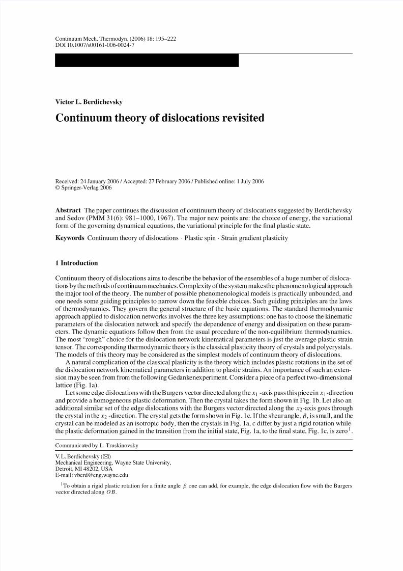
A natural complication of the classical plasticity is the theory which includes plastic rotations in the set of the dislocation network kinematical parameters in addition to plastic strains. An importance of such an exten-sion may be seen from from the following Gedankenexperiment. Consider a piece of a perfect two-dimensionallattice (Fig. 1a).
Let some edge dislocations with the Burgers vector directed along the x 1 -axis pass this piecein x 1-direction
and provide a homogeneous plastic deformation. Then the crystal takes the form shown in Fig. 1b. Let also anadditional similar set of the edge dislocations with the Burgers vector directed along the x 2-axis goes throughthe crystal in the x 2 -direction. The crystal gets the form shown in Fig. 1c. If the shear angle, β, is small, and thecrystal can be modeled as an isotropic body, then the crystals in Fig. 1a, c differ by just a rigid rotation whilethe plastic deformation gained in the transition from the initial state, Fig. 1a, to the final state, Fig. 1c, is zero1.
Communicated by L. Truskinovsky
V. L. Berdichevsky (B)Mechanical Engineering, Wayne State University,Detroit, MI 48202, USAE-mail: [email protected]
1To obtain a rigid plastic rotation for a finite angle β one can add, for example, the edge dislocation flow with the Burgersvector directed along O B.
From the perspective of the classical plasticity theory which takes into account only plastic deformations, suchrigid plastic rotation is unnoticeable and does not affect any relation of the theory. In reality, the initial and
the final states of the crystal are different: the dislocations passing through the crystal heat the crystal, and thetemperature must be higher in the final state. We see that the plastic rotation must be taken into account toobtain the adequate energy balance.
We can draw another important conclusion from this Gedankenexperiment. The dislocations passingthrough the crystal do not change the orientation of the crystal lattice in space. The material coordinatesystem rotates, however. Therefore, the tensors determining the crystal anisotropy rotate with respect to thematerial frame. Such rotation is caused by the plastic flow. As a result, the internal energy density becomesan explicit function of the plastic distortion. The two effects mentioned do not depend on the size of the bodyand should be taken into account for microcsopic, mesoscopic and macroscopic bodies. It is apparent that theaveraged plastic rotations should be a part of the kinematic description of the dislocation networks, and thecorresponding plasticity theory must be modified accordingly (this is discussed in Sects. 2 and 5; see especiallyformula (93)).
To simplify the treatment in the introduction to this paper, we constraint it with geometrically linear theory
(i.e. a theory with linear kinematics); the nonlinear theory will be considered further in the body of the paper.All tensors in the linear theory are referred to a Cartesian frame with the coordinates x i , small Latin indicesi, j, k , l run through the values 1, 2, 3; summation over the repeated indices is implied.
Plastic rotations appear in the kinematical description of individual dislocations, and penetrate further nat-urally into the macroscopic continuum description of the dislocation networks. Each dislocation may be char-acterized by the tensor of plastic distortion, Ai j . Its deviation from the identity transformation, βi j ≡ Ai j −δi j ,δi j being the Kronecker delta, is defined as follows: let ui be the displacement vector field from the perfect
lattice to the defected one, and bi = [ui ] ≡ u+i − u−
i the jump of the displacements on the slip surface (± signs mark the limit values of the displacements on the two sides of the slip surface). Then, by definition,
where n j are the components of the unit normal vector directed from the side − of the surface to the side+, δ() the δ-function of the surface
δ() =
δ( x − x )d A
δ( x ) the usual three-dimensional δ-function, d A the area element on . The definition (1) does not dependon the way one marks the sides of the slip surface: denoting the side − by + yields the simultaneous changeof the signs of the Burgers vector and the normal vector leaving the product in (1) invariant 2. For brevity, wecall the tensor βi j the tensor of plastic distortion as well.
Plastic strains, ε( p)
i j , and plastic rotations, ωi j , are the symmetric and antisymmetric parts of the plastic
distortion:
ε( p)
i j = 1
2(βi j + β ji ) ≡ β(i j ), ωi j = 1
2(βi j − β ji ) ≡ β[i j], βi j = ε
( p)
i j + ωi j . (2)
Round and square brackets in indices denote symmetrization and skew-symmetrization, respectively.Nye [2] introduced an important characteristic of dislocations, the dislocation density tensor,
αi j = e jk l ∂k βil (3)
Here e jk l the Levi–Civita symbol, ∂k ≡ ∂/∂ x k , partial derivatives will be also denoted by the comma inindices: ∂k βil ≡ βil ,k . There is an identity (see Kunin [3,4])
e jk l ∂k (nl δ()) = τ j δ() (4)
being the dislocation line, the boundary of the slip surface , τ j the tangent vector to , δ() the delta-function of the line ,
δ() =
δ( x − x s )ds,
ds the arc length along . Therefore, for an individual dislocation we have
αi j = bi τ j δ(). (5)
The first problem which arises here is to find the stress field for a given set of dislocations. If bi = constalong the slip surfaces, the stress field depends only on the positions of the dislocation lines; the shapes of the slip surfaces do not affect the stress field. A general solution of the problem was given by Kröner [5]. Anelegant treatment in terms of the generalized functions was suggested by Kunin [3,4].
A nonlinear generalization of the theory is based on the idea by Kondo [6,7] and Bilby (see [8–10]) to con-sider the unloaded space as a manifold with an affine connection. The dislocation field is characterized by themetric tensor of the manifold (that is equivalent to plastic strains), the curvature tensor and the torsion tensor.Bilby argued that for crystal lattices the curvature tensor must vanish; then the only kinematic characteristicsare the metric tensor and the torsion tensor, the latter being equivalent to the dislocation density tensor. Thisset of kinematic characteristics is equivalent to just plastic distortions: In the linear case the plastic strains
and the dislocation density tensor can be found from (2) and (3); the inverse statement is also true: the plasticdistortion can be found if the plastic strains and the dislocation density tensor are known (Le and Stumpf [11]).Kondo considered a more general case when the curvature tensor is not zero. Then the torsion (dislocationdensity tensor) cannot be expressed in terms of plastic distortion and becomes an independent field. This lineof thought seems not being pursued further though it has some merits. In what follows we assume the zerocurvature of the unloaded space. Thus, plasticity kinematics is characterized by the plastic distortion only, andthe dislocation density tensor is determined by the plastic distortion from Eq. (3).
2 Note that usually one defines the Burgers vector in a different way: on the same slip plane, for a fixed choice of the normalvector, one takes the orientation of the boundary of , the dislocation line, to be seen in the counter clock-wise direction fromthe top of the normal vector; then the sign of the Burgers vector is chosen in such a way that the triad {normal vector, tangentvector to the dislocation line, Burgers vector} be right oriented. Though the signs of the Burgers vector for the definition givenin the text and the usual definition can be different, the plastic distortions are the same, and this is the only what matters in ourtreatment.
As soon as the kinematics is fixed one can apply the methods of non-equilibrium thermodynamics to obtainthe governing equations. This was done by Sedov and Berdichevsky [1]3. The equations of continuum theoryof dislocations were derived in [1] using the variational approach [13]. They will be rederived here from thestandard thermodynamic reasoning in a simplified setting.
In thermodynamic and variational approaches the model is specified by choosing the expressions for energyand dissipation. The example model considered in [1] has the following energy density per unit volume, U ,and dissipation density, D, which we present here in their linear version and neglect, for simplicity, someinteraction terms:
U = U 0
ε
(e)i j , S
+ U m, (6)
U m = 1
2 E i j kl αi j αkl (7)
D =
K i j kl ε( p)
i j ε( p)
kl + M i j kl αi j αkl
12
(8)
Here ε(e)
i jare the elastic strain tensor components:
ε(e)i j = εi j − ε
( p)
i j , εi j = 1
2(ui, j + u j,i ), (9)
S the entropy density, U 0 the elastic energy, dot denotes the time derivative. The coefficients E i j kl , K i j kl , M i j kl
are some material constants.The relevance of this model to describing the behavior of the dislocation networks was not clear. The major
concern was the smallness of the second term in (6). To estimate its order denote the characteristic value of the constants E i j kl by E (they have the dimension of the shear modulus, µ, times length squared) and by l
the corresponding characteristic length: l =( E /µ)1/2. The order of the dislocation density tensor, α, can be
obtained by noting that αi j can be written in terms of the elastic distortion, β(e)i j = ui, j − βi j :
αi j
= −e jk l ∂k β
(e)
il(10)
Assuming that the elastic distortion is of the same order as the elastic strains, ε(e), we get an estimate of thedislocation density in terms of ε(e) and the characteristic length of the problem, L : α ∼ ε(e)/ L . So, the two
terms in (6) are of the orders µ
ε(e)2
and µl2(ε(e)/ L)2, respectively. If they are of the same order,
µ
ε(e)2
∼ µl2
ε(e)
L
2,
then the characteristic lengths l and L must be also of the same order 4,
l ∼ L .
In a polycrystal, we have at hand a number of material characteristic lengths: the interatomic distance, b, theaverage distance between dislocations, the average dislocation cell size, the average grain size. If one identifiesl with any of these distances, then in a macroscopic problem L l, and the second term in (6) is negligiblein comparison with the first one. Similar conclusion can be made with respect to the second term in (8). Theproblems with mesoscopic and microscopic values of L were not seen at the time, and the theory was notpursued further. Recently an interest to such type of problems has appeared motivated mostly by the experi-mentally observed intrinsic and extrinsic size effects on micro-level. A number of models have been suggested[14–28] 5. The applicability and the meaning of continuum models on small scales are complicated issues
3 The same paper was published also in the conference proceedings [12]. Only one publication will be cited further.4 Unless there is a large coefficient in E i j k l . There are no reasons to assume such a coefficient.5 Gurtin [25] arrived in linear case to the same equations as given in [1]. The models proposed in [14–28] differ too much to be
all physically relevant. Perhaps, the homogenization analysis of the dislocation network dynamics will determine which modelsfrom this variety are physically adequate.
(see the discussion in [29,30]); presumably, a continuum description could make sense for laminar plasticflows. Note that the question on the physical meaning of the characteristic material length still does not have
a convincing answer6.The above-mentioned difficulty seems to have been overcome, at least partially, by a proposition about the
microstructure energy, U m, made in [32]. It was shown that the microstructure energy, U m, which includesthe interaction energy between dislocations and the self-energy of dislocations is, in fact, a function of localcharacteristics of dislocations only, in spite of the long-range character of the dislocation interactions. Themicrostructure energy can be modeled in the following way. The simplest local characteristic of the dislo-cation network is the scalar dislocation density, ρ, the total length of the dislocation lines per unit volume.An advantage of this characteristic is that the state without dislocations corresponds to the zero value of ρ.One may assume that the microstructure energy is a function of ρ. Dislocation density cannot be bigger thansome saturated value, ρs. A rough estimate of ρs is ρs ∼ 1/b2. It corresponds to the material completely filledwith dislocations. In fact, ρs is considerably less: if the dislocation density becomes too high in polycrystals,then the processes set on which are not accounted for in the continuum theory of dislocations and reduce thedislocation density—the new grain boundaries develop and the average grain size drops. In energy terms, thatmeans that, for a fixed average grain size, energy becomes very large if ρ ∼ ρs. On the other hand, for smallρ, energy is linear in ρ at least because the energy of dislocation cores is linear in ρ. A simple model function
which fits to these features of energy is [32]
7
U m = k µ ln1
1 − ρρs
. (11)
Theorderof magnitudeof thematerialconstants k , ρs wasestimatedforAlandNiask ∼ 10−4, ρs ∼ 1014-m−2.The link to the continuum theory of dislocations is provided by the following remark: the total dislocation
density, ρ, is a sum of the dislocation density of the stored dislocations, ρst, and the dislocation density of moving dislocations, denote it by α/b. The parameter α can be modeled in the isotropic case as
α = c1αi j αi j + c2αi j α ji (12)
c1, c2 being some phenomenological constants on the order of unity. Finally, one can put in (11)
ρ = ρst + αb
. (13)
Formulas (6),(11)–(13) determine the dependence of energy on the dislocation density tensor assumingthat the material parameters ρs and ρst are given and do not change in the course of deformation.
Note that the ratio α/bρs ∼ ε(e)/bρs L is small: even for L ∼ 10−4 m assuming ε(e) ∼ 10−4, b ∼ 10−10 m,ρs ∼ 1014 m−2 we have α/bρs ∼ 10−4. If we linearize Eq. (11) and keep only the leading terms, we obtain
U m = k µ
b(ρs − ρst)
c1αi j αi j + c2αi j α ji + k µ ln
1
1 − ρst
ρs
. (14)
Here we assumed that ρs − ρst ∼ ρs. Due to the smallness of α/bρs, the “square root term”8 is much biggerthan the quadratic term,
α
bρs
2 = 1
(bρs)2(c1αi j αi j + c2αi j α ji ).
6 There was an interesting attempt [31] to justify formula for energy (6). It was concluded that the characteristic length has themeaning of the average distance between dislocations. Unfortunately, the derivation contains a flaw which renders an incorrectresult. This will be discussed in detail elsewhere.
7 Though the particular form of the microstructure energy (11) is not essential in the derivation of the governing equations, itis convenient for various estimates. Consider here the following one. An infinite value of the microstructure energy for ρ = ρs is,of course, an approximation which may be valid away from this point. In fact, energy is very large and finite for ρ = ρs. One can
modify(11) as U m = k µ ln[1/(1+ −ρ/ρs)] andseek for thecorresponding valueof thecorrection, . Let ρs ∼ 1/b2. If ρ = ρs,i.e. the dislocations occupy all the body, then the microstructure energy is on the order of the energy of a "melted body" which
can be estimated as λ/b2, λ being the energy of the dislocation core per unit dislocation length. Hence, = exp[−λ/k µb2]. For
the typical values λ ∼ 1−ev/b, µb3 ∼ 5−ev and for k ∼ 10−4, is very small: ∼ exp[−2.5 × 10⁵].8 Energy as a linear function of the square root term appeared for the first time, perhaps, in [33].
Nevertheless, linearization and neglecting the quadratic term is not always justifiable: this changes consid-erably the properties of the model. The model with energy (14) allows the plastic distortion to have discontinu-ities: the total energy remains finite for discontinues plastic distortions. Energy (11) as well as the energy (7)prohibits the discontinuities becoming infinite for the discontinuous plastic distortions. Due to that the model
with energy (11) allows one to capture such features as, for example, the structure of the dislocation pile-upsat the grain walls.Note that the last term in (14) is quite essential. It describes the energy of the stored dislocations. This
energy is huge, and, in fact, may be much bigger than the elastic energy. For example, for ρst = 0.1ρs, thestored dislocation energy is in the order of 10−5µ while the elastic energy for ε(e) = 10−4 is in the orderof 10−8µ. Therefore, even small changes in stored dislocation density has a profound effect on the energybalance, and taking into account the evolution of the stored dislocation density may be much more importantthan the incorporation in the theory the gradients of plastic distortion. Perhaps, the exceptions are an initialstage of plastic flow, an easy glide, when ρst 0, and the development of geometrically necessary dislocations.
In contrast to the two effects illustrated by Fig. 1, the dependence of energy density on αi j is essentialmostly for small bodies (or small characteristic length L). There is, however, a reason why this dependencemay be of importance for macroscopic bodies as well: the leading term in energy, elastic energy, in linearapproximation does not depend on plastic rotations, and the only term containing plastic rotations is U m(αi j ).Therefore, even being small, it becomes the leading one in determination of the plastic rotation field.
Non-equilibrium thermodynamics describes, in particular, the evolution of closed systems to their equi-librium states. According to the Gibbs variational principles, the equilibrium states are the states with themaximum value of entropy (for fixed energy) and/or the states with the minimum value of energy (for fixedentropy). The choice of energy in a theory shapes the structure of the entire non-equilibrium theory becauseit determines the “fixed points” of the dynamic equations. In case of plasticity this has the following implica-tions: if one gives some displacements to the boundary points of a plastic body and keeps these displacementsconstant, then a plastic flow develops which drives the energy to its minimum value and stops when the energytakes this value. Our choice of energy specifies which final states will develop. If the final states are reachedfast enough, one may neglect the transitional process and consider only the final states. They are determinedby minimization of energy. One such problem concerning the development in the body the geometricallynecessary dislocations will be considered in Sect. 3.
In what follows we give a rederivation of the equations of the paper [1] from the reasoning of non-equilib-rium thermodynamics in geometrically linear case (Sect. 2) and geometrically nonlinear case (Sect. 4), considera variational problem for determining the geometrically necessary dislocations in one constrained shear prob-lem (Sect. 3), and suggest an energy expression for finite plastic deformation which depends explicitly onplastic distortion (Sect. 5).
2 Geometrically linear continuum theory of dislocations
2.1 System of equations
By geometrically linear continuum dislocation theory we mean the approximation of small displacements,small plastic distortions and their gradients (i.e. they all can be neglected in comparison with unity or the cor-responding characteristic length or inverse length). In such theory one can disregard the differences between theLagrangian and Eulerian coordinates. The theory to discussion of which we proceed is based on the following
assumption: the energy of the crystal possesses the energy density which is a function of only local character-
istics – elastic strains, ε(e)
i j = εi j − ε( p)
i j , plastic distortions, βi j , dislocation density tensor, αi j = e jk l ∂k βil ,
and entropy per unit mass, S :
U = U
S , ε(e)
i j , βi j , αi j
. (15)
In what follows we denote by U the energy density per unit mass. Entropy S is understood here in a usualsense as the thermodynamic entropy of thermal motion of atoms of the crystal lattice. There might be situationswhen energy depends also on the configurational entropy of the dislocation network (see [30,32]), but suchcases are beyond the scope of this paper.
Let V 0 be a subregion in the initial state of the crystal; it coincides with the corresponding actual positionof this subregion in the deformed state within the framework of the linear theory. The energy of the crystal
Here ρ0 is the mass density in the initial state which coincides with the actual mass density in the deformedstate in a linear theory.
Let the crystal be adiabatically isolated. Besides, we assume for simplicity that the heat conductivity isnegligible, i.e. for any region V 0 there are no heat flux through the boundary ∂ V 0 of the region V 0. Then thefirst law of thermodynamics states that the energy rate is equal to the power of the external forces:
d
dt
V 0
ρ0U
S , ε(e)i j , βi j , αi j
dV = P. (17)
The structure of the power is controlled by the form of the energy. For example, if U depended only on S and
ε(e)
i j = u(i, j ) − β(i j ), and, thus, only the space derivatives of displacements entered the energy density, then
P = ∂ V 0
σ i j n j ui d A,
where dot denotes the time derivative, n j the components of unit normal vector at ∂ V 0, and σ i j , the componentsof the stress tensor, are some functions of space coordinates and time. In general, if U were dependent on thegradients of some parameter, ϕ, then there are some "generalized stresses", σ i , such that
P =
∂ V 0
σ j n j ϕd A.
The origin of such a special structure of the power has the deep roots in the Gibbs variational principles;it is explained also by Sedov’s variational equation [13].
In our case, due to the assumed form of the internal energy, the power should have the form
P =
∂ V 0
σ i j n j ui + σ i jk nk βi j
d A. (18)
We see that some stresses of higher order, σ i jk , enter into the theory as a result of the dependence of energydensity on the gradients of plastic distortion.
Transforming the surface integral in (18) into the volume integral by means of the divergence theorem, weobtain from (16)–(18) the equation:
V 0
ρ0
∂U
∂ S S + ρ0
∂U
∂ε(e)i j
(u(i, j ) − β(i j )) + ρ0∂U
∂βi jβi j + ρ0
∂U
∂αi j
e jk l ∂k βil
−σ i j
˙ui, j
−σ i j, j
˙ui
−σ i jk βi j,k
−σ i jk ,k βi jdV
=0 (19)
Since the region V 0 is arbitrary, this equation may be satisfied only if the integrand is zero identically.Employing the standard notation, T , for the derivative, ∂U /∂ S , which is the absolute temperature,
Here we used that, due to the symmetry of the derivatives, ∂U /∂ε(e)i j ,
ρ0∂U
∂ε(e)i j
u(i, j ) = ρ0∂U
∂ε(e)i j
ui, j , ρ0∂U
∂ε(e)i j
β(i, j ) = ρ0∂U
∂ε(e)i j
βi, j .
For rigid translational motion, entropy, S , and stresses, σ i j , do not change while ui, j and βi j are zero.Therefore, in order the first law of thermodynamics to be fulfilled, the stresses must obey to the equilibriumequations:
σ i j, j = 0. (22)
For rigid rotations, i.e. for arbitrary u[i, j], entropy and stresses do not change as well, while u(i, j ) and βi j
are zero. The first law of thermodynamics can be satisfied only for symmetric stress tensor,
σ i j = σ ji (23)
Let us introduce the following notation:
τ i j = σ i j − ρ0 ∂U ∂ε
(e)
i j
, τ i jk = σ i jk − ρ0 ∂U ∂αim
emk j , (24)
i j = ρ0∂U
∂ε(e)i j
− ρ0∂U
∂βi j
+ σ i jk ,k . (25)
Then, the first law of thermodynamics takes the form:
ρ0T S = τ i j ui, j + i j βi j + τ i jk βi j,k (26)
Equations (24), (26) show that the tensors τ i j , τ i jk are the parts of the stresses σ i j and the higher orderstresses σ i jk which cause heating of the crystal. To emphasize that the stresses contain two parts, the one relatedto energy and irrelevant to heating and the another one which causes heating, we rewrite the Eqs. (24) in theform:
σ i j = ρ0∂U
∂ε(e)
i j
+ τ i j , σ i jk = ρ0∂U
∂αim
emk j + τ i jk . (27)
Tensor τ i j describes heating in a non-uniform flow, and, thus, has the meaning of viscous stresses. It is
symmetric due to symmetry of σ i j and ∂U /∂ε(e)
i j . Tensors i j and τ i jk describe heating which is caused by
homogeneous and inhomogeneous plastic deformation, respectively.A widely used closure of non-equilibrium thermodynamics, which satisfies the Onsager reciprocal rela-
tions in linear case, assumes that the right hand side of Eq. (26), the dissipation, D, is a given function of ui, j , βi j , βi j,k ,
9:
ρ0T S = D ui, j , βi j , βi j,k (28)
andthatthethetensors τ i j , i j , τ i jk controlling the irreversible processes in the crystal are linked toui, j ,βi j , βi j,k
by the relations:
τ i j = λ∂ D
∂ ui, j
, i j = λ∂ D
∂βi j
, τ i jk = λ∂ D
∂βi j,k
(29)
Then the parameter λ is determined from (26), (29):
λ = D
∂ D
∂ui, jui, j + ∂ D
∂βi j
βi j + ∂ D
∂βi j,k
βi j,k
. (30)
9 and, possibly, the arguments of the energy density; the latter are not mentioned explicitely among the arguments of thedissipation function.
Some relaxed versions of the potential relations (29) are also possible [1].It is worthy to emphasize that, in contrast to the Onsager reciprocal relations, the potential law (29) is not a
“law of Nature” (see [34]). However, the potential law seems to cover most of the currently employed modelsof plasticity.
For a given internal energy, U
S , ε(e)
i j , βi j , αi j
, and dissipation, D
ui, j , βi j , βi j,k
, the Eqs. (22), (23),(25), (26 ), (20) along with the constitutive equations (27)–(30 ) and the kinematic formulas (2), (3), (9), forma closed system of equations.
In what follows we ignore the viscous effects; accordingly, dissipation does not depend on the velocitygradients, and viscous stresses vanish
τ i j = 0.
2.2 Dissipation potential
The major physical motivation to use the potential form of the constitutive equations (29) is the Onsagerreciprocal relations of linear thermodynamics. In the nonlinear region one may use other nonlinear equations
which yield the Onsager reciprocal relations in the linear case. As such we will use the assumption on theexistence of the dissipation potential, D, such that
i j = ∂D
∂βi j
, τ i jk =∂D
∂βi j,k
. (31)
The dissipation potential is linked to the dissipation by the formula
∂D
∂βi j
βi j + ∂D
∂βi j,k
βi j,k = D.
For homogeneous dissipation of the order m, i.e. for the function D(βi j , βi j,k ) possessing the property:for any positive number, µ,
D(µβi j , µβi j,k ) = µm
D(βi j , βi j,k ),
the equality holds
∂ D
∂βi j
βi j + ∂ D
∂βi j,k
βi j,k = m D,
thus, the constant λ (30) is equal to 1/m. Hence, the Eqs. (31) and (29) coincide for
D = D
m. (32)
In general, the Eqs. (31) and (29) are different. There are no physical reasons at the moment to prefer (31)or (29). Equations (31) possess, however, one advantage: the constitutive equations can be written in a verycompact and beautiful “variational” form:
δD
δβi j
= σ i j − ρ0δU
δβi j
, σ i j = ρ0∂U
∂ε(e)
i j
. (33)
Here the notation for the variational derivative is used: for any function ϕ(u, u, u,i ),
Equations (33) can be checked by inspection. According to these equations, the inclusion of gradients of βi j in U and gradients of βi j in D yields only one change in the equations: the usual partial derivatives mustbe changed by the variational derivatives.
In (33), the derivatives of U with respect to βi j are computed when the elastic strains are fixed. If the
derivatives of U with respect to βi j for fixed total strains, εi j , are used, δεU /δβi j , then the equations servingto determine βi j take especially simple form:
δD
δβi j
= −ρ0δεU
δβi j
. (34)
Note also that Eqs. (33) retain their form if energy density depends on all the gradients of plastic distortion,not only on their anti-symmetric part, αi j , as we assumed in the derivation.
2.3 Plastic incompressibility
If the plastic distortion obeys some kinematic constraints, the equations change accordingly. The case of plastic
incompressibility,
βii = 0 (35)
is especially interesting.We are going to show that the equations serving to determine βi j for plastic incompressible flows can be
written in the form:
δD
δβ i j
= σ i j − ρ0δU
δβi j
(36)
where prime denotes the deviatoric part of the tensor, e.g. σ i j = σ i j − 1/3σ kk δi j .
There are two key points in the derivation of equations (36). The first one is the meaning of the derivatives
∂U /∂ε
(e)
i j , ∂U /∂βi j in case when ε
(e)
i j and βi j obey to some constraints. Consider first the symmetry constraintfor the strain tensor, ε
(e)
i j , and take an example: U is a quadratic form of a two-dimensional symmetric tensor
ε(e)
i j ,
U = 1
2ε
(e)i j ε
(e)i j = 1
2
ε
(e)11 ε
(e)11 + 2ε
(e)12 ε
(e)12 + ε
(e)22 ε
(e)22
.
If we take the derivatives of this function in the usual sense,
∂U
∂ε(e)11
= ε(e)11 ,
∂U
∂ε(e)12
= 2ε(e)12 ,
∂U
∂ε(e)22
= ε(e)22
they do not form the components of a tensor. To get a tensor, we must take derivatives of function U with
respect to ε(e)i j as if this tensor is not symmetric; such derivatives,
∂U
∂ε(e)11
= ε(e)11 ,
∂U
∂ε(e)12
= ε(e)12 ,
∂U
∂ε(e)21
= ε(e)21 ,
∂U
∂ε(e)22
= ε(e)22
do form a tensor. The similar remark pertains to the other constraints as well, in particular, to the incompress-ibility constraint (35). Energy and dissipation in this case must be defined not only for the incompressibleplastic fields, but for all fields as if these fields could be compressible. Incompressibility implies that βi j entersin U only through the combination,
Computing the derivatives of U and D we admit all fields, not only the incompressible ones. Thus,
∂U
∂βi j
= ∂U
∂β i j
− 1
3
∂U
∂β kl
δkl δi j =
∂U
∂βi j
(37)
and, similarly,
∂ D
∂βi j
= ∂ D
∂β i j
− 1
3
∂ D
∂β kl
δkl δi j =
∂ D
∂β i j
,
∂ D
∂βi j,k
= ∂ D
∂β i j,k
− 1
3
∂ D
∂β ml ,k
δml δi j =
∂ D
∂β i j,k
The equations for βi j (31) are replaced by the equations:
i j =
∂D
∂
˙β
i j
, τ i jk =
∂D
∂
˙β
i j,k
(38)
Therefore, the tensors i j and τ i jk automatically have zero traces:
ii = 0, τ ii k = 0 (39)
According to Eq. (27), the scalar, ii /3, has the meaning of “plastic pressure”, and the assumptions madeyield zero plastic pressure.
Equations (37) and (38) can be further simplified if we accept that energy and dissipation possess theproperty: for any constants λ and λk
U
β i j + λδi j , β
i j,k + λk δi j
= U
βi j , β
i j,k
,
(40)
D
β
i j + λδi j , β i j,k + λk δi j
= D
β
i j , β i j,k
Such a property is not fulfilled automatically (it is enough to consider a linear function, ai j β i j , were tensorai j has a non-zero trace), but it is not physically constraining since it can be achieved by the correspondingredefinition of thearguments of energy and dissipation (inthe above example of a linear function, we replace thetensor ai j by a
i j ; then energy satisfies to the condition (40) and has the same values as before). Differentiating
(40) with respect to λ and λk we obtain the identities
∂U
∂βi j
δi j = 0,∂U
∂βi j,k
δi j = 0,∂D
∂β i j
δi j = 0,∂D
∂β i j,k
δi j = 0
and, hence,
i j = ∂D
∂βi j
, τ i jk =∂D
∂β i j,k
(41)
One can check that the Eqs. (36) follow from (33) and (41).The second point concerning the derivation of (36) is that the rule of computation the derivatives describedabove is not a pure mathematical issue: it has a physical origin. Usually, the constraints have a physical nature:the unconstrained deformation is possible but yields either very large energy or very large dissipation, and,therefore, is not realized. Accepting the plastic incompressibility constraint we ignore the dislocation climb.In order to justify Eqs. (36) one should consider a more complete theory which allows the dislocation climb tooccur. Such theory should include also the additional required fields, concentrations of vacancies and intersti-tial atoms which are responsible for the volume change and accompany the dislocation climb. An asymptoticanalysis of this more complete theory will presumably yield the equations formulated10. Such a derivationseems not have been attempted though11.
10 In particular, in such asymptotic analysis one should presumably obtain that plastic pressure is negligible compared withelastic pressure.
11 A similar problem, the transition from slightly compressible fluid to incompressible fluid, was considered in [35].
For a wide range of plastic flows, the plastic deformation may be viewed as rate independent. That meansthe following. Consider homogeneous plastic deformation, βi j (t ) (βi j,k = 0). Let βi j = Bi j (t ) be a closed
deformation loop in the space of βi j -variables, t 0 ≤ t ≤ t 1, Bi j (t 0) = Bi j (t 1). The total dissipation (thetotal amount of heat generated in the course of deformation along this loop) is equal to
t 1 t 0
D ˙ Bi j (t )
dt . (42)
Forrate independent flow, the total dissipation is the same for all flows βi j = Bi j (θ (t )) with any functionθ (t ), θ(t 0) = t 0, θ (t 1) = t 1. We accept additionally that dissipation does not change if the direction of flowis reversed, D(−βi j ) = D(βi j ). It is easy to see that dissipation must be a first-order homogeneous function
of βi j for the rate independent flows. The dissipation potential, D, and dissipation, D, coincide for the rateindependent flows.
Dislocation motion is governed by usual rate dependent (primary) thermodynamics. Macroscopic crystal
plasticity is an averaged description of dislocation networks, and, thus, is a subject of the next level thermody-namics called secondary in [34]. The mechanism of the development the rate independence in the transitionfrom the primary to the secondary thermodynamics was explained by Puglisi and Truskinovsky [36].
Independence of the integral (42) on the strain rate forany deformation path is a far going three-dimensionalgeneralization of a quite restricted set of one-dimensional experiments. In any case, it is the base of classicalplasticity. Von Mises plasticity theory corresponds to the dissipation
D = D = K
β
(i j )β
(i j )(43)
and the internal energy,
U = U S , ε(e)i j . (44)
In the case of the von Mises dissipation (43) and the internal energy (44) the equations to determine plasticdeformations,(36), take the form:
K β (i j )
β (kl )β
(kl )
= σ i j
The anti-symmetric part of (36) is satisfied automatically.For the general energy density (15) and dissipation (43), Eqs. (36) form a system of nine equations,
and the tree equations which are anti-symmetric with respect to i, j
δU
δβi j
− δU
δβ ji
= 0. (47)
Equations (47) may be considered as equations serving to determine the plastic rotations, βi j −β ji . Plasticrotations remain undetermined in von Mises theory and similar theories of classical plasticity. In continuumtheory of dislocations with energy (6), (7), plastic rotations are determined uniquely. It is worthy to emphasizethat including into the theory the microstructure energy, U m, even (7) which is small compared to the elasticenergy, is essential for determining the plastic rotations: according to the general rules of asymptotic analysisof functionals depending on small parameters [35,37], only those small terms can be neglected for which thebigger ones depending on the same variables can be found. Since the plastic rotations enter only in U m, themicrostructure energy is the leading term depending on plastic rotations and, therefore, cannot be neglected.In terms of equations (47), this means that, though only small terms contribute to these equations, they cannotbe neglected because they all are of the same order.
For β (i j )
= 0, as follows from (45), the stresses must obey the condition:
σ i j − ρ0
δU
δβ(i j )
σ i j − ρ0
δU
δβ(i j )
= K 2
. (48)
This is a cylindrical “yield surface” in the stress space. The term ρ0δU /δβ(i j )
describes translational work
hardening.If
β(i j ) = 0 (49)
then the left hand side of (45) contains an uncertainty of the type 0 /0. In this case, the equation (45) arereplaced by (49).
As was mentioned in Introduction, dissipation must depend on the plastic spin 13, β[kl ]. In the case of rateindependent isotropic plasticity we have
D = K 21 β (i j )β (i j ) + K 22 β[i j]β[i j]. (50)
The Eqs. (46) and (47) are replaced by the equations:
K 21 β (i j )
K 21 β (i j )
β (i j )
+ K 22 β[i j]β[i j]= σ i j − ρ0
δU
δβ(i j )
(51)
K 22 β[i j] K 21 β
(i j )β
(i j )+ K 22 β[i j]β[i j]
= −ρ0δU
δβ[i j](52)
Similarly to the previous case, for β i j = 0, the stresses must lie on the yield surface
1
K 21
σ i j − ρ0
δU
δβ(i j )
σ i j − ρ0
δU
δβ(i j )
+ 1
K 22ρ0
δU
δβ[i j]ρ0
δU
δβ[i j]= 1. (53)
The second term in the left hand side indicates that the dependence of energy on plastic rotations resultsin some decrease of the yield stress.
The experimental values of the constants, K 1 and K 2, seem not known. The Gedankenexperiment describedin Sect. 1 suggests that these constants must be of the same order. If this is indeed the case, then for the plasticflows satisfying the condition ρ0
δU
δβi j
ρ0δU
δβi j
σ i j σ i j
, (54)
13 It was called in [1] the plastic whirl. The term "plastic spin" is commonly accepted nowadays.
the rate of plastic rotations is much smaller than that of plastic strains. If initially β[i j] = 0, then β[i j] ≈ 0 in
the course of deformation14. The inequality (54) is plausible for the macro-samples with energy (7) or (11),(12), but it does not hold for micro-samples. This inequality may be also violated if the Bauschinger effect istaken into account.
If the dissipation is a function like (8) then, for M i j kl = 0, the yield surface becomes a surface in thespace of variables σ i j , τ i jk . The scope of physical mechanisms which are covered by such models has not been
revealed yet.
2.5 Dissipation in rate dependent plasticity
According to the rate independent plasticity the plastic deformation do not develop until stresses reach theyield surface; besides, stresses cannot exceed the yield stress. Both features do not correspond to reality: plasticdeformations may develop at any value of stresses, and, due to the external forces, stresses in the body canbe made much higher then the yield stress. This discrepancy is caused by the approximate nature of the rateindependence hypothesis. In fact, there is a rate dependence which is weak for small stresses but becomes quitepronounced for high stresses. A way to take the rate dependence into account is to modify the dissipation. In
the case of von Mises dissipation (43) we put
D = K
β (i j )β
(i j )
12 (1+ 1
m)
. (55)
Here m is a big number. In the limit m → ∞, dissipation ( 55) tends to von Mises dissipation (43). Function(55 ) is a homogeneous function of 1 + (1/m) order; according to (32), the dissipative potential is
D = D
1 + 1m
= K
1 + 1m
β
(i j )β (i j )
12 (1+ 1
m)
.
The flow rule, (36) becomes:
K β (i j )
β
(i j )β (i j )
121−
1
m =
σ i j
−ρ0
δU
δβi j
. (56)
The antisymmetric part of equations (56) is again (47) while the symmetric one is
K β (i j )
β (i j )
β (i j )
12
1− 1
m
= σ i j − ρ0δU
δβ(i j )
. (57)
To determine an analogue of the yield surface in this model it is worthy to resolve equations (57) withrespect to the strain rate. First, we have from (57):
K 2 β(i j )β
(i j )1/m =
σ i j − ρ0δU
δβ(i j )
σ i j − ρ0
δU
δβ(i j )
.
Hence,
β (i j )β
(i j ) =
1
K 2
σ i j − ρ0
δU
δβ(i j )
σ i j − ρ0
δU
δβ(i j )
m
and
β (i j ) = 1
K
σ i j − ρ0
δU
δβ(i j )
1
K 2
σ kl − ρ0
δU
δβ(kl )
σ kl − ρ0
δU
δβ(kl )
12 (m−1)
.
14 From other reasoning this conclusion was made by Dafalias [38]. It was used by Bassani [22] in constructing a model of strain gradient plasticity. Similar point was made also by Gurtin [25].
The similar modification of the dissipation (50) is
D =
K
2
1+ 1m
1 β(i j )β
(i j ) + K
2
1+ 1m
2 β[i j]β[i j]
12 (1+ 1
m )
.
Then again D = D/(1 + 1m
), and
K
2
1+ 1m
1 β (i j )
K 2
1+ 1m
1 β (i j )
β (i j )
+ K 2
1+ 1m
2 β[i j]β[i j] 1
2 (1−1
m ) =σ i j
−ρ0
δU
δβ(i j )
K
2
1+ 1m
2 β[i j]K
2
1+ 1m
1 β (i j )
β (i j )
+ K
2
1+ 1m
2 β[i j]β[i j]
12 (1− 1
m)
= ρ0δU
δβ[i j]
.
The magnitude of plastic rate is determined by the value of the function
1
K
2
1+ 1m
2
σ i j
−ρ0
δU
δβ(i j )σ i j
−ρ0
δU
δβ(i j )+
1
K
2
1+ 1m
2
ρ0δU
δβ[i j]ρ0δU
δβ[i j] .
The plastic rate becomes finite if this function is equal to unity, and huge if it exceeds unity.Now we proceed to the discussion of the issues which do not depend on the character of dissipation.
3 Plastic deformation and energy minimization
Consider a crystal the boundary displacements of which, u(b)
Functions u(b)i are assumed to be continuous, therefore no dislocations enter into the crystal in the course of
deformation. Accordingly, at the boundary15
βi j = 0. (59)
Equation (59) models, e.g., a situation at a high angle grain boundary when stresses are not large enough topush the dislocations through the boundary.
If we wait long enough, the crystal will arrive at the state with the minimum value of energy, ˇ E . In crystalswith negligible resistance to dislocation motion, like pure copper, such state can be reached very fast.
The minimum value of energy is determined from the variational problem:
ˇ E = minui ∈(58)
βi j ∈(59)
V 0
ρ0U
S , ε(e)i j , βi j , αi j
dV (60)
where minimum is sought with respect to all displacement fields obeying to the boundary conditions (58) andall plastic distortions which are zero at the boundary16. We assume also that energy density does not dependon plastic distortion explicitly,
U = U
S , ε(e)
i j , αi j
,
besides, it is a strictly convex function of ε(e)
i j and αi j , and the minimum value of U (S , ε(e)
i j , αi j ) is achieved
when ε(e)i j and αi j are zero.
The functional to be minimized is convex but not strictly convex functional of displacements and plasticdistortion: its value does not change if one make a “compatible plastic shift”,
ui → ui + u( p)
i , βi j → βi j + ∂u( p)
i
∂ x j(61)
where u( p)
i ( x i ) are arbitrary functions. The minimizing functions in the variational problem (60) are determined
up to an arbitrary compatible plastic shift, u( p)i ( x i ), which satisfies the boundary conditions:
u( p)
i = 0,∂u
( p)
i
∂ x j= 0 at ∂ V 0.
The dynamics of the plastic flow determines the plastic shift uniquely. Usually, it depends on the history of deformation. There are situations, however, when the final state is determined uniquely and independently onthe deformation history due to the additional constraints for the plastic distortion caused by a special orientationof the slip planes. Here we consider one such example.
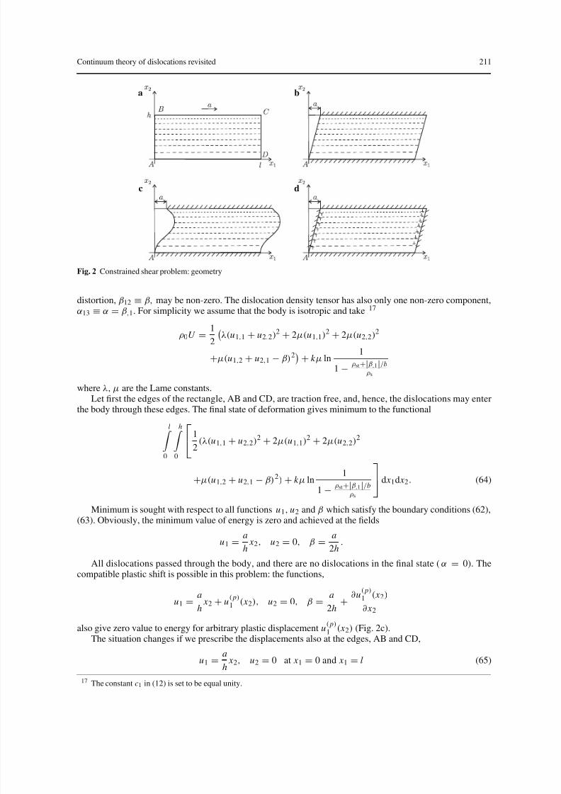
Let the deformation does not depend on the coordinate x 3, and the cross-sections of the body by the planes x 3 =const is a rectangle, 0 ≤ x 1 ≤ l, 0 ≤ x 2 ≤ h. We clamp the bottom side of the rectangle,
u1
=u2
=0 at x 2
=0 (62)
and shift the top side:
u1 = a, u2 = 0 at x 2 = h (63)
(see Fig. 2a). Let the plastic deformation is possible only along the planes x 2 =const (they are shown inFig. 2 by dash lines); at these planes the edge dislocations may appear. So, only one component of the plastic
15 More precisely, the boundary displacements are assumed to be the same both on micro- and macro-levels. The boundarycondition (59) is a consequence of continuity of the microscopic displacement field: due to (1), if a slip plane crosses the bound-ary there is a jump of displacements at the boundary, and βi j = 0 at the boundary. In principle, in a macroscopic theory, themacroscopic displacement field may be continuous even for non-zero βi j at the boundary.
16 Not all boundary conditions (59) may be essential in the minimization problem, i.e. removing some of the constraints (59)may not alter the minimum value. We do not pay attention to this issue here because the functional determines itself whichboundary conditions it must respect.
distortion, β12 ≡ β, may be non-zero. The dislocation density tensor has also only one non-zero component,α13 ≡ α = β,1. For simplicity we assume that the body is isotropic and take 17
ρ0U = 1
2
λ(u1,1 + u2,2)2 + 2µ(u1,1)2 + 2µ(u2,2)2
+µ(u1,2 + u2,1 − β)2+ k µ ln
1
1 − ρst+|β,1|/b
ρs
where λ, µ are the Lame constants.Let first the edges of the rectangle, AB and CD, are traction free, and, hence, the dislocations may enter
the body through these edges. The final state of deformation gives minimum to the functional
l 0
h 0
1
2(λ(u1,1 + u2,2)2 + 2µ(u1,1)2 + 2µ(u2,2)2
+µ(u1,2 + u2,1 − β)2) + k µ ln1
1 − ρst+|β,1|/b
ρs
d x 1d x 2. (64)
Minimum is sought with respect to all functions u1, u2 and β which satisfy the boundary conditions (62),(63). Obviously, the minimum value of energy is zero and achieved at the fields
u1 = a
h x 2, u2 = 0, β = a
2h.
All dislocations passed through the body, and there are no dislocations in the final state ( α = 0). Thecompatible plastic shift is possible in this problem: the functions,
u1 = a
h x 2 + u
( p)
1 ( x 2), u2 = 0, β = a
2h+ ∂u
( p)
1 ( x 2)
∂ x 2
also give zero value to energy for arbitrary plastic displacement u( p)
1 ( x 2) (Fig. 2c).The situation changes if we prescribe the displacements also at the edges, AB and CD,
u1 = a
h x 2, u2 = 0 at x 1 = 0 and x 1 = l (65)
17 The constant c1 in (12) is set to be equal unity.
Dislocations cannot enter the body through the boundary. We have to set
β = 0 at x 1 = 0 and x 1 = l (66)
Dislocations may be nucleated only inside the body (in neutral pairs) so that the total Burgers vector at
each slip plane is zero due to the boundary conditions (66):
l 0
αd x 1 =l
0
∂β
∂ x 1d x 1 = 0
Now the minimum of the functional (64) must be sought under the additional constraints, (65) and (66).
The constraints (65) and (66) eliminate the kernel of energy: if U = 0, and, hence, ε(e)11 = ε
(e)12 = ε
(e)22 = α = 0,
then the required functions, u1, u2, and β are also zero. It follows from the equations
u1,1 = 0, u2,2 = 0, u1,2 + u2,1 − β = 0, β,1 = 0
and the boundary conditions (62), (63), (65), (66). Therefore, the minimizing functions are unique.The problem formulated does not seem to admit an analytical solution. However, qualitatively one may
expect the following behavior: for sufficiently small shear, γ ≡ a/ h, the body deforms purely elastically,and β ≡ 0. If the shear exceeds some critical value, γ ∗, then the dislocations nucleate to reduce the energy,and β becomes non-zero. Dislocations will accumulate near the boundaries (Fig. 2d). Such expectations aresupported by the following approximate solution. Since u1 − ax 2/ h and u2 vanish at the boundary, we mayassume that, approximately, they are equal to zero everywhere in the strip
u1 ≡ ax 2
h, u2 ≡ 0 (67)
while β is a function of only longitudinal coordinate, x 1.On such fields the functional (64) becomes a functionalof β( x 1) only:
ˇ E
=min
β( x 1)∈(66)
hµ
l
01
2
(γ
−β)2
+k ln
1
1 − ρst+β, x 1/b
ρs
d x 1. (68)
It is convenient to make a change of the variables,
β = γ u( x ), x 1 = ax , a ≡ γ
b(ρs − ρst).
The new independent dimensionless variable, x , changes on the segment [0, L], L = l/a. The variationalproblem takes the form:
ˇ E = hµlk ln1
1 − ρst
ρs
+ hµaγ 2(m), m ≡ k
γ 2
(m) = minu( x ):
u(0)=u( L)=0
I (u),
I (u) = L
0
1
2(1 − u( x ))2 + m ln
1
1 −u, x
d x . (69)
Consider first the linearized version of the microstructure energy:
I (u) = L
0
1
2(1 − u( x ))2 + mu, x
d x (70)
The major difference between (69) and (70) is that the minimizing function of the functional (69) mustbe smooth (derivatives, u, x , cannot exceed unity) while the minimizing function of the functional (70) may
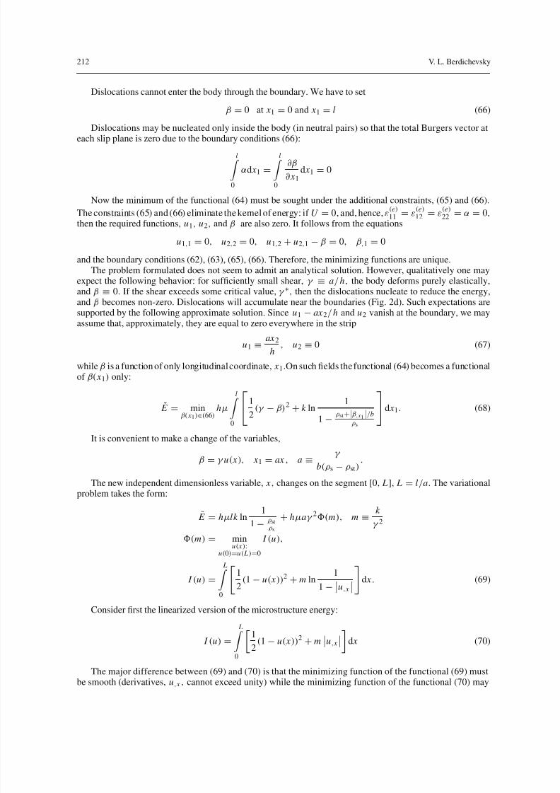
Fig. 3 Dependence of the plastic strain on the total shear strain
have discontinuities, and each discontinuity, [u], gives a contribution to the functional equal to m |[u]| . Theminimizing functions of the functional (70) are piece-wise constant functions. Indeed, if u, x = 0 in a vicinityof some point, then the integrand in (70) is differentiable, and one can write the Euler equation for (70) whichgives u = const: we come to contradiction. Hence, u, x = 0. The functional (70) is strictly convex, therefore ithas the only minimizing function. This function cannot have jumps inside the segment [0, L] : ifit does and hasat some point x ∗ a jump, then moving x ∗ in the direction where (1 − u)2 is bigger, we decrease the functional,and such a function cannot provide the minimum value. So, the jumps may be only at the end points. Denoteby u the constant value of u( x ) inside the segment. The functional is a function of one variable, u :
I (u) = 1
2(1 − u)2 L + 2m |u| .
Its minimum value is
(m) =
2m
1 − m L
if 2m
L≤ 1
L2 if 2m
L≥ 1
.
It is achieved for
u =
1 − 2m L
if 2m L
≤ 1
0 if 2m L
≥ 1
.
This justifies the statement made: the dislocations do not appear (u = 0) until shear exceeds some criticalvalue. For the critical value we have
2m
L =2ka
γ ∗2l =2k
γ ∗bl(ρs − ρst) =1
thus,
γ ∗ = 2k
bl(ρs − ρst).
The dependence of plastic deformation, β, on the external shear, γ , is shown in Fig. 3.This simple model describes geometrical hardening, kind of Hall–Petch effect: the shorter the strip the
larger shear must be to initiate the plastic deformation. After overcoming the threshold there is no work hardening in the course of deformation: the growth of the plastic shear strain,
Such a behavior is caused by linearization of the problem. In case of the original functional (69) one wouldobserve the work hardening as well.
The role of the logarithmic term in (69) is that it prohibits the jumps, and transforms the jumps into theboundary layers. We consider here the boundary layer near x = 0. To this end it is enough to put in (69) L = ∞ and drop the boundary condition u( L) = 0. We obtain the variational problem,
minu( x ):
u(0)=0
∞ 0
1
2(1 − u( x ))2 + m ln
1
1 −u, x
d x (71)
The minimizing function increases from zero to unity, therefore u, x > 0, and the sign of the absolute valuein (71) can be dropped. Denote by p( x ) the function
p( x ) = d
du, x
m ln1
1 − u, x
= m
1 − u, x .
The minimizing function satisfies the boundary value problem:
d p
d x = u − 1,
du
d x = 1 − m
p, u(0) = 0, u(∞) = 1. (72)
Function p( x ) is a decreasing function of x . Since du/d x → 0 at infinity, p(∞) = m.The system (72) admits the first integral,
1
2 (1 − u( x ))2
+ m ln p − p = const.
The value of the constant can be found from the conditions at infinity:
1
2(1 − u( x ))2 + m ln p − p = m ln m − m.
Hence,
1 − u( x ) =
2m
p( x )
m− 1 − ln
p( x )
m
. (73)
The expression under the square root is positive because p( x ) ≥ m and x ≥ ln x + 1 for x ≥ 1. Finally, forthe function q( x ) = p( x )/m − 1, we have the initial value problem
dq
d x = −
2
m(q − ln(1 + q)), q(0) = q0
where, according to (73), q0 is the solution of the equation
q0 − ln(1 + q0) = 1
2m.
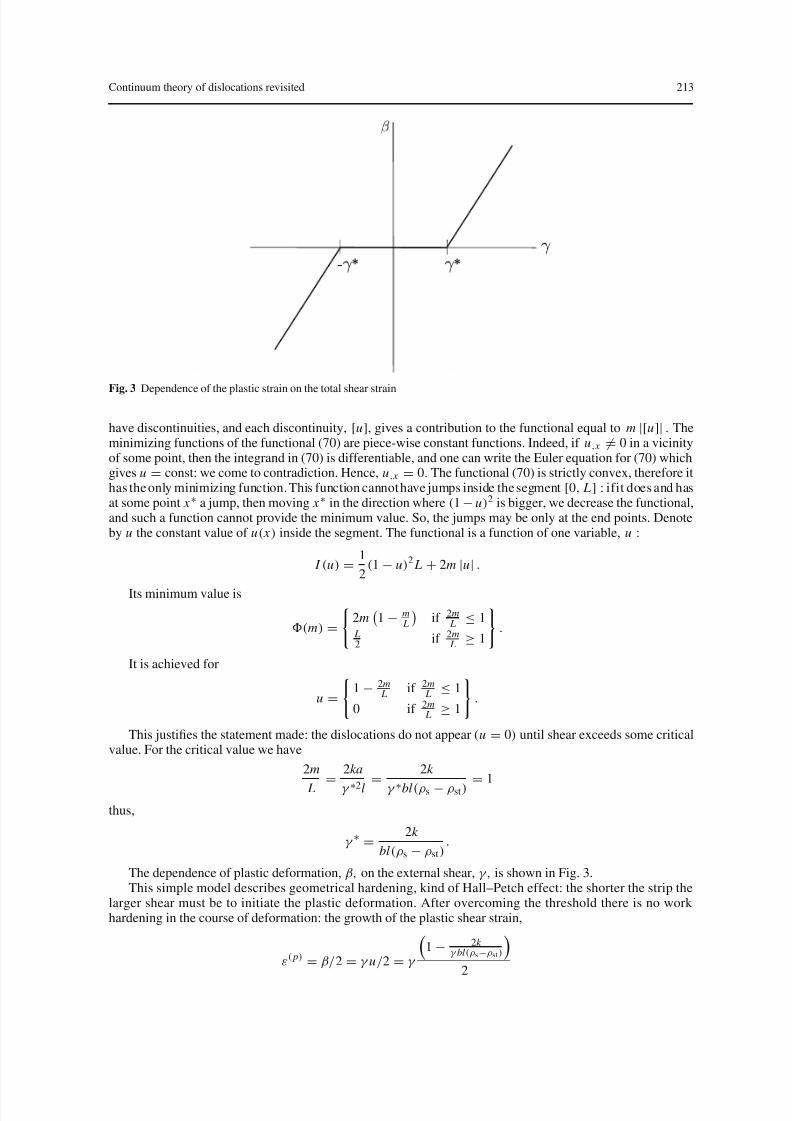
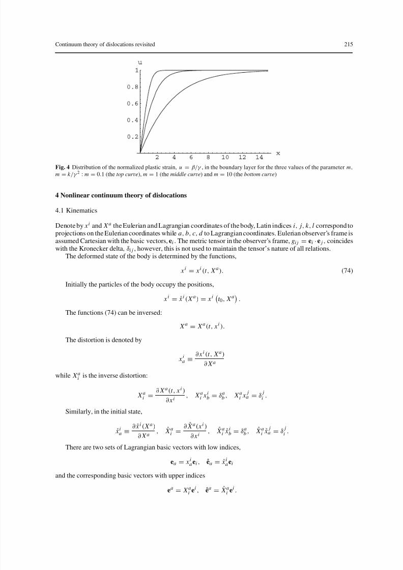
The dependence of the normalized plastic distortion, u( x ) = β/γ, is shown in Fig. 4 for the three valuesof m = k /γ 2.
Fig. 4 Distribution of the normalized plastic strain, u = β/γ , in the boundary layer for the three values of the parameter m,
m = k /γ 2 : m = 0.1 (the top curve), m = 1 (the middle curve) and m = 10 (the bottom curve)
4 Nonlinear continuum theory of dislocations
4.1 Kinematics
Denote by x i and X a the Eulerian and Lagrangian coordinates of the body, Latin indices i, j, k , l correspond toprojections on the Eulerian coordinates while a, b, c, d to Lagrangian coordinates. Eulerian observer’s frame isassumed Cartesian with the basic vectors, ei . The metric tensor in the observer’s frame, gi j = ei ·e j , coincideswith the Kronecker delta, δi j , however, this is not used to maintain the tensor’s nature of all relations.
The deformed state of the body is determined by the functions,
x i = x i (t , X a ). (74)
Initially the particles of the body occupy the positions,
x i
= ˚ x i
( X a
) = x i
t 0, X a
.
The functions (74) can be inversed:
X a = X a (t , x i ).
The distortion is denoted by
x ia ≡ ∂ x i (t , X a )
∂ X a
while X ai is the inverse distortion:
X a
i =∂ X a (t , x i )
∂ x i, X a
ix i
b =δa
b, X a
ix
j
a =δ
j
i.
Similarly, in the initial state,
˚ x ia ≡ ∂ ˚ x i ( X a )
∂ X a, ˚ X ai = ∂ ˚ X a( x i )
∂ x i, ˚ X ai ˚ x ib = δa
b , ˚ X ai ˚ x j
a = δ ji .
There are two sets of Lagrangian basic vectors with low indices,
ea = x ia ei , ea = ˚ x ia ei
and the corresponding basic vectors with upper indices
For a plastically deformed body, one introduces one more set of vectors, e∗a (t , X a ), which is the result of
the following thought procedure: one cuts off a small piece of material in the vicinity of the point X a andunload it; then vectors ea (t , X a ) transform into vectors e∗
a (t , X a ). The components of the vectors e∗a (t , X a)
are denoted by Aia ,
e∗a = Ai
a (t , X a)ei
These nine fields, Aia (t , X a ), describe the kinematics of plastic deformation. The inverse tensor is denoted
by Bai ,
ei = Bai e∗
a , e∗a = Bai ei , Ai
a Ba j = δi
j , Aia Bb
i = δba
The Eulerian indices are moved by means of the metric tensor gi j .There are three metric tensors in the Lagrangian frame,
gab = gi j x ia x j
b , g∗ab = gi j Ai
a A jb, gab = gi j ˚ x ia ˚ x
jb
and, accordingly, the three measures of strains: total strains,
εab = 1
2
gab − gab
(75)
elastic strains,
ε(e)ab = 1
2
gab − g∗
ab
(76)
and plastic strains,
ε( p)
ab = 1
2
g∗
ab − gab
. (77)
Total strain is the sum of elastic and plastic strains,
εab = ε(e)ab + ε
( p)ab . (78)
To measure strains as the differences, (75)–(77), is feasible if the strains are small, otherwise metric tensorsare the adequate measures of deformations themselves. In crystal plasticity, the elastic strains are small whilethe plastic strains can be large. This corresponds to smallness of the difference, ea− e∗
a = ( x ia − Aia )ei .
Incompatibility of the plastic deformation is measured by the tensor, Ai[a,b]. To have all its components in
one coordinate system, we put
αab = Bai εbcd Ai
d ,c. (79)
Here εbcd are the contravariant components of the Levi–Civita tensor in the Lagrangian frame:εbcd = ebcd /
√ g, ebcd the Levi–Civita symbols, g being the determinant of the matrix ||gab|| .
Three comments concerning the motivation for the notation chosen are in order to conclude this subsection.
1. The continuum mechanics equations are invariant with respect to the two groups of transformations: trans-formations of the observer’s frames,
x i = x i ( x j ) (80)
and transformations of the Lagrangian frames,
X a = X a ( X b). (81)
The group (80) causes the transformation of Eulerian indices, i, j, k , l, while the objects with the Lagrang-ian indices, a, b, c, d , are not affected by this group and behave as scalars. Similarly, the group (81) yieldsthe transformations of the objects with the Lagrangian indices leaving the objects with the Eulerian indicesunchanged. This is why one needs to distinguish these two types of indices in the notation.
2. An alternative would be to use the direct tensor notation when, for example, for a vector, one writes v,implying that v =vi ei . Unfortunately, the attractive simplicity of the direct notation is accomponied bysome shortcomings. Dealing with the components of a vector we do not know the vector. This is empha-sized by the formula v =vi ei : to prescribe a vector one needs to specify both the components, vi , and
the frame, ei . For the same components of, say, the elastic strain tensor (75), one can define three differenttensors
ε1 = ε(e)
ab ea eb, ε2 = ε(e)
ab ea eb, ε3 = ε(e)
ab e∗a e∗b.
We are interested in the dependence of energy on the components of the strain tensor, not on the entiretensor itself: it does not matter whether the strain tensor is the tensor ε1, ε2 or ε3. If we, nevertheless, writeU = U (ε1), we introduce into energy the extra arguments, the basic vectors, on which energy, in fact, doesnot depend. Mathematically, nothing is wrong: function may be independent on some of the arguments, butphysically, this complication does not seem reasonable. Another shortcoming with the formula U = U (ε1)is that one has to list all other arguments of energy, and the form of the arguments not mentioned may affectthe function U (ε1).For example, in the case of an isotropic media the additional argument is just a tensorof the second order formed from the metric tensor. We have, however, a number of possibilities:
g1 = gab ea eb, g2 = gab ea eb, g3 = g∗ab eaeb, g4 = gab ea eb
not to mention a few more. The models with energies, say, U = U (ε1, g1) and U = U (ε1, g2) are different.For example, in the case of the linear dependence of energy on the elastic strains,
U (ε1, g1) = const gab ε(e)
ab , U (ε1, g2) = const gab ε(e)
ab
These are two different functions. Without specifying the additional arguments in energy the model remainsundetermined. These issues are not essential in a linear theory but becomes important in nonlinear ones. Of course, after all necessary specializations, the direct notation makes sense; however, such specializationsare needed only because we introduced the artificial argument into energy, the basic vectors. This is whythe author prefers the index notation which avoids any ambiguities.
3. One can introduce the elastic distortion, the transition from the vectors e∗a
to the vectors ea
, and the plasticdistortion, the transition from vectors ea to vectors e∗
a , by the formulas
ea = F (e)ba e∗
b, e∗a = F
( p)ba eb.
These distortions are linked to the distortions used, x ia and Aia , by the relations:
x ia = F (e)ba Ai
b, Aia = F
( p)ba ˚ x ib.
The elastic and plastic distortions, F (e)b
a and F ( p)b
a , can be expressed in terms of distortions x ia and Aia :
F (e)ba = Bb
i x ia , F ( p)b
a = ˚ X bi Aia.
The total distortion is a multiplication of elastic and plastic distortions,
x ia = F (e)ba F
( p)cb ˚ x ic. (82)
The measure of elastic strains, ε(e)ab , can be expressed in terms of elastic distortions as:
ε(e)ab = 1
2
gi j F (e)c
a Aic F
(e)d b A
jd − g∗
ab
= 1
2g∗
cd
F (e)c
a F (e)d
b − δcaδd
b
(83)
The decomposition of the total distortion, x ia, into the product of elastic and plastic distortions was firstintroduced by Bilby, et al. [39] and further discussed by Kröner [40] and Lee [41]. The distortions used here, x ia and Ai
a , seem more convenient in the development of the general relationships.
Now we repeat the derivation of the basic equations of the Sect. 2 in the nonlinear setting. The energy densityis assumed to be a function of entropy density, total and plastic distortions and the dislocation density tensor:
U = U
S , x ia , Aia , αab
. (84)
There are additional arguments of energy which do not depend on time and, thus, are not listed among thearguments. These are the components of some tensors L
a1a2...as
1 , ..., which describe the physical propertiesof the media. It is essential that the components of all tensors are taken in Lagrangian coordinates. One canuse the Eulerian components of the tensors as well, but in this case, the physical characteristics of the body,
Li1i2 ...is
1 = x i1a1
x i2a2 ... x
isas
La1a2 ...as
1 , ..., are dependent on the deformation, and the form of the equations becomes
unnecessary complicated. Energy may depend on the initial distortion, ˚ x ia , which also does not change in time.So, for total energy of body we have
E = V 0
ρ0U
S , x ia , Ai
a , αab
dV
where dV =
gd X 1d X 2d X 3, g being the determinant of the initial metric, g = detgab
. The power of theexternal forces acting at the boundary of the body is
P =
∂ V 0
(σ j
i n j vi + σ a ji n j
˙ Aia )d A.
Here vi is the particle velocity,
vi ≡ ∂ x i (t , X a )
∂t
In the same way as in Sect. 2 one obtains the equilibrium equations (22), the symmetry of the stress tensor(23), the constitutive equations (further equations are given under the assumption that the viscous stresses arezero),
σ j
i = ρ0∂U
∂ x ia x
jb − ∂U
∂α cd αcd δ
ji (85)
ai = −ρ0
∂U
∂ Aia
+ ρ0∂U
∂αcd αad Bc
i + σ a ji, j (86)
σ aj
i = ρ0∂U
∂α cd Bc
i εdba x j
b + τ a ji (87)
and the equation for entropy,
ρ0T S =
a
i ˙ A
i
a + τ
a j
i ˙ A
i
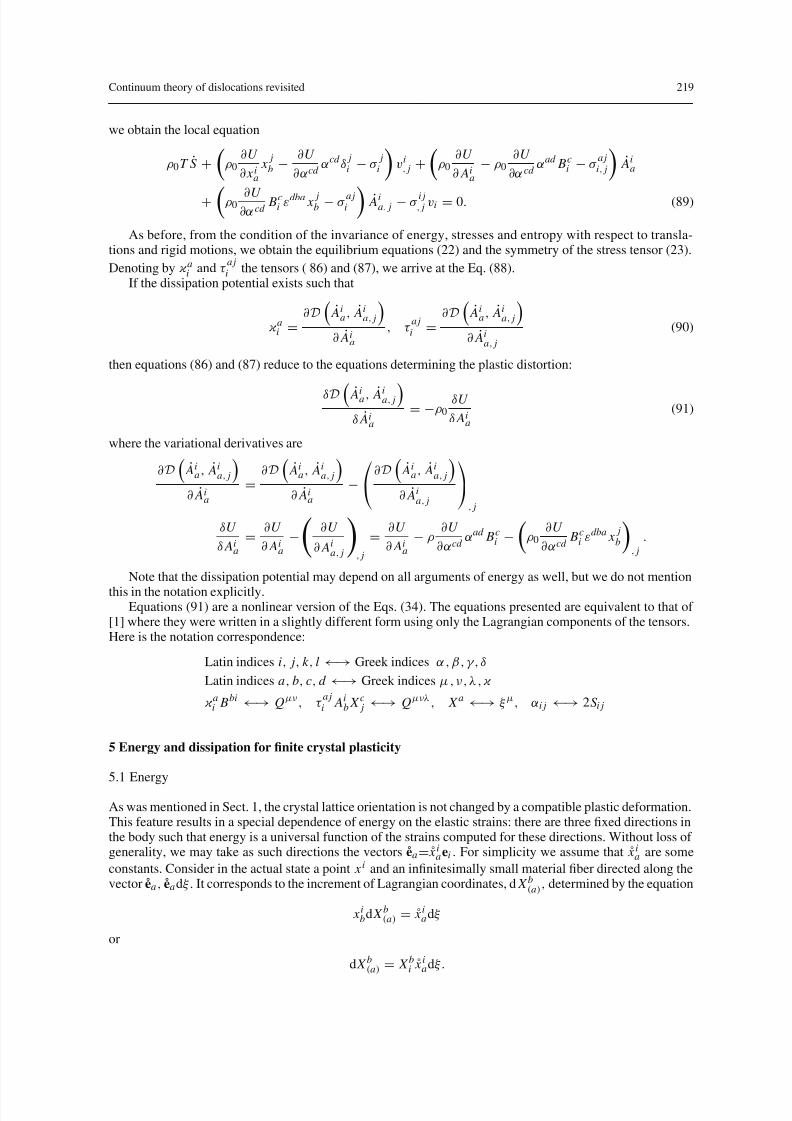
a, j . (88)
The derivation proceeds as follows. First, note the kinematical relations for the time derivatives:
As before, from the condition of the invariance of energy, stresses and entropy with respect to transla-tions and rigid motions, we obtain the equilibrium equations (22) and the symmetry of the stress tensor (23).
Denoting by ai and τ
a ji the tensors ( 86) and (87), we arrive at the Eq. (88).
If the dissipation potential exists such that
ai =
∂D
˙ Aia , ˙ Ai
a, j
∂ ˙ Ai
a
, τ a ji =
∂D
˙ Aia , ˙ Ai
a, j
∂ ˙ Ai
a, j
(90)
then equations (86) and (87) reduce to the equations determining the plastic distortion:
δD ˙ Aia , ˙ Aia, j
δ ˙ Aia
= −ρ0δU
δ Aia
(91)
where the variational derivatives are
∂D
˙ Aia , ˙ Ai
a, j
∂ ˙ Ai
a
=∂D
˙ Aia , ˙ Ai
a, j
∂ ˙ Ai
a
−∂D
˙ Aia , ˙ Ai
a, j
∂ ˙ Ai
a, j
, j
δU
δ Aia
= ∂U
∂ Aia
−
∂U
∂ Aia, j
, j
= ∂U
∂ Aia
− ρ∂U
∂αcd αad Bc
i −
ρ0∂U
∂αcd Bc
i εdba x j
b
, j
.
Note that the dissipation potential may depend on all arguments of energy as well, but we do not mention
this in the notation explicitly.Equations (91) are a nonlinear version of the Eqs. (34). The equations presented are equivalent to that of
[1] where they were written in a slightly different form using only the Lagrangian components of the tensors.Here is the notation correspondence:
Latin indices i, j, k , l ←→ Greek indices α , β , γ , δ
Latin indices a, b, c, d ←→ Greek indices µ, ν , λ ,
ai Bbi ←→ Qµν , τ
a ji Ai
b X c j ←→ Qµνλ , X a ←→ ξ µ, αi j ←→ 2S i j
5 Energy and dissipation for finite crystal plasticity
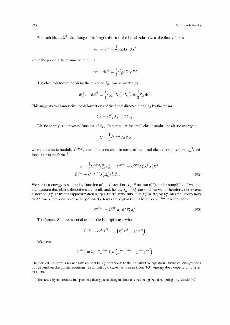
5.1 Energy
As was mentioned in Sect. 1, the crystal lattice orientation is not changed by a compatible plastic deformation.This feature results in a special dependence of energy on the elastic strains: there are three fixed directions inthe body such that energy is a universal function of the strains computed for these directions. Without loss of generality, we may take as such directions the vectors ea= ˚ x ia ei . For simplicity we assume that ˚ x ia are some
constants. Consider in the actual state a point x i and an infinitesimally small material fiber directed along thevector ea , ea dξ. It corresponds to the increment of Lagrangian coordinates, d X b
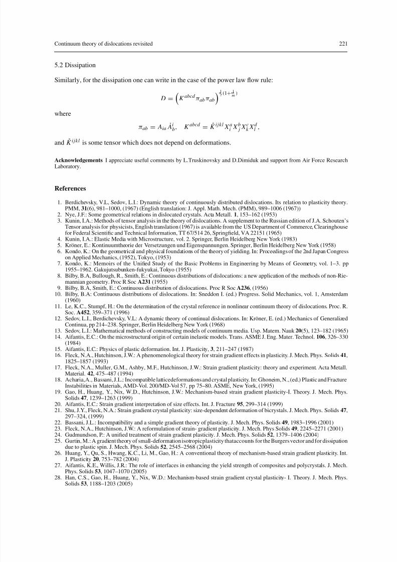
Similarly, for the dissipation one can write in the case of the power law flow rule:
D = K abcd πab πab 12 (1
+1m
)
where
πab = Aia˙ Ai
b, K abcd = K i j kl X ai X b j X ck X d l ,
and K i j kl is some tensor which does not depend on deformations.
Acknowledgements I appreciate useful comments by L.Truskinovsky and D.Dimiduk and support from Air Force ResearchLaboratory.
References
1. Berdichevsky, V.L, Sedov, L.I.: Dynamic theory of continuously distributed dislocations. Its relation to plasticity theory.PMM, 31(6), 981–1000, (1967) (English translation: J. Appl. Math. Mech. (PMM), 989–1006 (1967))
2. Nye, J.F.: Some geometrical relations in dislocated crystals. Acta Metall. 1, 153–162 (1953)3. Kunin, I.A.: Methods of tensor analysis in the theory of dislocations. A supplement to the Russian edition of J.A. Schouten’s
Tensor analysis for physicists, English translation (1967) is available from the US Department of Commerce, Clearinghousefor Federal Scientific and Technical Information, TT 67/514 26, Springfield, VA 22151 (1965)
4. Kunin, I.A.: Elastic Media with Microstructure, vol. 2. Springer, Berlin Heidelberg New York (1983)5. Kröner, E.: Kontinuumtheorie der Versetzungen und Eigenspannungen. Springer, Berlin Heidelberg New York (1958)6. Kondo, K.: On the geometrical and physical foundations of the theory of yielding. In: Proceedings of the 2nd Japan Congress
on Applied Mechanics, (1952), Tokyo, (1953)7. Kondo, K.: Memoirs of the Unified Study of the Basic Problems in Engineering by Means of Geometry, vol. 1–3. pp
1955–1962. Gakujutsubunken-fukyukai, Tokyo (1955)8. Bilby, B.A, Bullough, R., Smith, E.: Continuous distributions of dislocations: a new application of the methods of non-Rie-
mannian geometry. Proc R Soc A231 (1955)9. Bilby, B.A, Smith, E.: Continuous distribution of dislocations. Proc R Soc A236, (1956)
10. Bilby, B.A: Continuous distributions of dislocations. In: Sneddon I. (ed.) Progress. Solid Mechanics, vol. 1, Amsterdam(1960)11. Le, K.C., Stumpf, H.: On the determination of the crystal reference in nonlinear continuum theory of dislocations. Proc. R.
Soc. A452, 359–371 (1996)12. Sedov, L.I., Berdichevsky, V.L: A dynamic theory of continual dislocations. In: Kröner, E. (ed.) Mechanics of Generalized
Continua, pp 214–238. Springer, Berlin Heidelberg New York (1968)13. Sedov, L.I.: Mathematical methods of constructing models of continuum media. Usp. Matem. Nauk 20(5), 123–182 (1965)14. Aifantis, E.C.: On the microstructural origin of certain inelastic models. Trans. ASME J. Eng. Mater. Technol. 106, 326–330
(1984)15. Aifantis, E.C.: Physics of plastic deformation. Int. J. Plasticity, 3, 211–247 (1987)16. Fleck, N.A., Hutchinson, J.W.: A phenomenological theory for strain gradient effects in plasticity. J. Mech. Phys. Solids 41,
1825–1857 (1993)17. Fleck, N.A., Muller, G.M., Ashby, M.F., Hutchinson, J.W.: Strain gradient plasticity: theory and experiment. Acta Metall.
Material. 42, 475–487 (1994)18. Acharia,A., Bassani, J.L.: Incompatible latticedeformations and crystal plasticity. In: Ghoneim, N., (ed.) Plastic and Fracture
Instabilities in Materials, AMD-Vol. 200/MD-Vol 57, pp 75–80. ASME, New York, (1995)
297–324, (1999)22. Bassani, J.L.: Incompatibility and a simple gradient theory of plasticity. J. Mech. Phys. Solids 49, 1983–1996 (2001)23. Fleck, N.A., Hutchinson, J.W.: A reformulation of strain- gradient plasticity. J. Mech. Phys Solids 49, 2245–2271 (2001)24. Gudmundson, P.: A unified treatment of strain gradient plasticity. J. Mech. Phys. Solids 52, 1379–1406 (2004)25. Gurtin, M.: A gradient theory of small-deformation isotropicplasticity thataccounts for the Burgers vector and for dissipation
due to plastic spin. J. Mech. Phys. Solids 52, 2545–2568 (2004)26. Huang, Y., Qu, S., Hwang, K.C., Li, M., Gao, H.: A conventional theory of mechanism-based strain gradient plasticity. Int.
J. Plasticity 20, 753–782 (2004)27. Aifantis, K.E., Willis, J.R.: The role of interfaces in enhancing the yield strength of composites and polycrystals. J. Mech.
29. Berdichevsky, V., Dimiduk, D.: On failure of continuum plasticity theories on small scales. Scripta Material. 52, 1017–1019(2005)
30. Berdichevsky, V.: Homogenization in micro-plasticity. J. Mech. Phys. Solids 53, 2457–2469 (2005)31. Popov, V.L., Kröner, E.: Theory of elastoplastic media with mesostructure. Theor Appl Fracture Mech. 37, 299–310 (2001)32. Berdichevsky, V.: On thermodynamics of crystal plasticity. Scripta Material. 54, 711–716 (2006)
33. Ortiz, M., Repetto, E.A.: Nonconvex energy minimization and dislocation structures in ductile single crystals. J. Mech. Phys.Solids 47, 397–462 (1999)34. Berdichevsky, V.L.: Structure of equations of macrophysics. Phys. Rev. E 68:066126 (2003)35. Berdichevsky, V.L.: Variational principles of continuum mechanics. Nauka, Mascow, (1983)36. Puglisi, G., Truskinovsky, L.: Thermodynamics of rate independent plasticity. J. Mech. Phys. Solids 53, 655–679 (2005)37. Berdichevsky, V.L.:Variational-asymptotic method of constructing shell theory. J. Appl. Math. Mech. (PMM) 44(4), 664–687
(1979)38. Dafalias, Y.F.: The plastic spin. J. Appl. Mech. 52, 865–871 (1985)39. Bilby, B.A., Gardner, L.R.T., Stroh, A.N.: Extraitdes Actes du IX Congrès Internationalde Mechanique Appliqueè, Bruxelles,