GEOSTATISTIC MAPPING OF ARSENIC, MANGANESE AND IRON CONTAMINATION RISK IN THE PORT OF SANTANA, AMAPA, BRAZIL Joaquim Carlos Barbosa Queiroz, Universidade Estadual Paulista, Brazil, José Ricardo Sturaro, Universidade Estadual Paulista, Brazil, and Paulina Setti Riedel, Universidade Estadual Paulista, Brazil ABSTRACT For over 4 decades intense industrial activity, brought on by manganese exploration and commercialization in Amapá, Brazil, produced profound changes in the region, both socially and environmentally. There are strong indications that a series of environmental problems caused by this activity, including surface and underground water contamination, mainly due to residue deposits produced at manganese pellet/sinter plant, in the industrial area of Santana, on the banks of the Amazon River, where the manganese is loaded on ships. From preliminary studies of surfac e and underground water samples, which showed concentrations of manganese, arsenic and iron above normal levels established for human health, an evaluation of the contamined water was done using geostatistic tools and stochastic simulation. Variografic models were used to describe the spatial continuity pattern for metal concentrations in the study. Conditional simulations, including annealing simulation, were done to evaluate the contamination level in unsampled areas, create risk maps showing contamination probabilities in the area and maps indicating established cut-off values. The results represented by pos-processe d maps of simulated values and global uncertainties showed the areas of higher contamination and more need of recovery. Manganese and arsenic demonstrated significantly higher results. The areas with higher levels of arsenic contamination are located in and around the fi ne refuse basin while manganese occupied a much large section, covering almost the entire study area, including a small portion outside the industrial area. INTRODUCTION There are many questions involving the problem of environmental contamination of surface and underground water. Generally , one seeks to find out when the concentration of a specific contaminant exceeds established standards, where the boundary lies between contaminated and uncontaminated areas, what the level of confidence is regarding those boundaries, how much contaminant (total mass) is present, and what needs to be removed. The main objective is to provide additional information beyond simple estimates of contamination in order to reduce the chances of any erroneous decisions. Up until the end of the 1980's, a typical geostatistical study was carried out in three steps: exploratory analysis of the da ta, modelling of the spatial variability (semivariogram), and finally, prediction of the attributes of values in locations where no samples were taken. It is now known, however, that algorithms of interpolation b y least square, such as kriging, tend to smooth out local details of spatial variation of the attribute, typically overestimating smaller values and underestimating larger values. The use of interpolated, smoothed-out maps is inappropriate for applications that are sensitive to the presence of extreme values and their patterns of continuity, such as the evaluation of sources of re-covering in mineral deposits (Journel & Alabert, 1990;
GEOSTATISTIC MAPPING OF ARSENIC, MANGANESE AND IRONCONTAMINATION RISK IN THE PORT OF SANTANA, AMAPA, BRAZIL
Joaquim Carlos Barbosa Queiroz, Universidade Estadual Paulista, Brazil,José Ricardo Sturaro, Universidade Estadual Paulista, Brazil,
and Paulina Setti Riedel, Universidade Estadual Paulista, Brazil
ABSTRACT
For over 4 decades intense industrial activity, brought on by manganeseexploration and commercialization in Amapá, Brazil, produced profound changes in theregion, both socially and environmentally. There are strong indications that a series ofenvironmental problems caused by this activity, including surface and undergroundwater contamination, mainly due to residue deposits produced at manganese
pellet/sinter plant, in the industrial area of Santana, on the banks of the Amazon River,where the manganese is loaded on ships. From preliminary studies of surface and
underground water samples, which showed concentrations of manganese, arsenic andiron above normal levels established for human health, an evaluation of the contaminedwater was done using geostatistic tools and stochastic simulation. Variografic modelswere used to describe the spatial continuity pattern for metal concentrations in the study.Conditional simulations, including annealing simulation, were done to evaluate thecontamination level in unsampled areas, create risk maps showing contamination
probabilities in the area and maps indicating established cut-off values. The resultsrepresented by pos-processed maps of simulated values and global uncertainties showedthe areas of higher contamination and more need of recovery. Manganese and arsenicdemonstrated significantly higher results. The areas with higher levels of arseniccontamination are located in and around the fine refuse basin while manganese occupieda much large section, covering almost the entire study area, including a small portionoutside the industrial area.
INTRODUCTION
There are many questions involving the problem of environmentalcontamination of surface and underground water. Generally, one seeks to find out whenthe concentration of a specific contaminant exceeds established standards, where the
boundary lies between contaminated and uncontaminated areas, what the level ofconfidence is regarding those boundaries, how much contaminant (total mass) is
present, and what needs to be removed. The main objective is to provide additionalinformation beyond simple estimates of contamination in order to reduce the chances ofany erroneous decisions.
Up until the end of the 1980's, a typical geostatistical study was carried out inthree steps: exploratory analysis of the data, modelling of the spatial variability(semivariogram), and finally, prediction of the attributes of values in locations where nosamples were taken. It is now known, however, that algorithms of interpolation by leastsquare, such as kriging, tend to smooth out local details of spatial variation of theattribute, typically overestimating smaller values and underestimating larger values.The use of interpolated, smoothed-out maps is inappropriate for applications that are
sensitive to the presence of extreme values and their patterns of continuity, such as theevaluation of sources of re-covering in mineral deposits (Journel & Alabert, 1990;
Nowak, Srivastava, & Sinclair, 1993), modelling of the flow of fluids in porousmediums (Schafmeister & De Marsily, 1993) or the delineation of contaminated areas(Desbarats, 1996; Goovaerts, 1997a). Stochastic simulation has increasingly becomethe method of choice for estimation due to the ease of generating maps realizations thatreproduce the sample variability, as opposed to interpolation methods that produced
maps estimated for one given criteria of optimization only. A set of realizations thatadjust reasonably well to the same statistics (histograms and semivariograms) is particularly useful to evaluate uncertainty about the spatial distribution of attributes ofvalues and to investigate the performance of various scenarios, such as mineral planningor remediation of pollution (Goovaerts, 1998). Although the principles of geostatisticalsimulation are known in the geostatistics literature, these techniques have not beenwidely applied to problems of contamination of underground water.
The realizations generated with conditional simulation techniques should honorthe data as closely as possible in order to be reliable numerical models for the attributeunder study. The application of optimization methods, such as annealing simulation
(AS), for stochastic simulation has the potential to honor the data more than theconventional geostatistical techniques of simulation. The essential characteristic of thisapproximation is the formulation of a stochastic image as a problem of optimizationwith some specific objective function. The data to be honored by the stochastic imagesare coded like components in an objective global function (Deustch, C. & Cockerham,P., 1994). There are various applications of annealing simulation in hydrogeology. Theapplication of AS to model stochastic aquafiers involves a two-step procedure: first, the
problem of interpolation is re-stated as a problem of optimization. Second, thisoptimization is solved using AS. Dougherty and Marryott (1991) were the first to applythis technique in the context of hydrogeology - the problem of optimization ofmanagement of underground water. In a later article, they deal with remediation ofunderground water in a contaminated area (Marryott, Dougherty, & Stollar, 1993).Deutsch and Journal (1991) applied AS in the stochastic modelling of reservoirs. Zengand Wang (1996) used AS to identify parameters of structure in the modelling ofunderground water (Fang & Wang, 1997).
In this study, we present an approximation using simulations to evaluate thecontamination of underground water with manganese, arsenic, and iron in the port cityof Santana, located in the state of Amapá in northern Brazil. AS was utilized, which is atechnique of flexible heuristic optimization commonly applied to obtain differentrealizations with specific spatial characteristics. The AS approximation requires no a
priori considerations regarding the base structure of the model, is not limited to randomGaussian fields, and does not require any functional form of the variogram (Gupta, et al,1995), making its use possible in situations where the variables have highlyasymmetrical distributions, such as the present study. A visual and quantitative measureof the spatial uncertainty is provided by the generation of numerous realizations(simulations) that adjust reasonably well to the same statistical samples (histogram andvariogram) and given conditions. Each realization is, therefore, consistent with theknown concentrations of contaminants, the sample histogram, and spatial continuitymodels exhibited by the data. Thus, each realization is an equally valid description ofcontamination. Probability summaries are prepared, based on the set of realizations, toobtain maps of risk that show the probability of contamination in the area under study,
to identify the location of boundaries between contaminated and uncontaminated zones,and to generate maps indicating the cut-off values established. Even if additional
significant information is obtained for decision-making regarding the evaluation ofcontaminated locations, this evaluation should always involve attention to the physical
processes responsible for the placement and, potentially, redistribution of thecontaminants.
ANNEALING SIMULATION
Simulated annealing is a generic name for a family of optimization algorithms based on the principle of stochastic relaxation (Geman & Geman, 1984). References forthe application of these techniques include Deutsch & Journel (1992), Deutsch &Cockerham (1994) and Goovaerts (1997). An initial image is gradually perturbed so asto match constraints such as the reproduction of target histogram and covariance whilehonoring data values at their locations. Unlike others simulation algorithms, the creationof a stochastic image is formulated as an optimization problem without reference to arandom function model. Geostastitical simulated annealing requires an objectivefunction that measures the deviation between the target and the current statistics of the
realization at each ith perturbation. Once the objective function has been established, thesimulation (actually an optimization) process amounts to systematically modifying aninitial realization so as to decrease the value of that objective function, getting therealization acceptably close to the target statistics. There are many possibleimplementations of the general simulated annealing paradigm. Variants differ in theway the initial image is generated and then perturbed, in the components that enter theobjective function, and the type of decision rule and convergence criteria that areadopted. In this study the initial image is generated honoring data values at theirlocations. The perturbation mechanism used is the swap the z -values at any two
unsampled locations u and u chosen at random, so becomes and
vice-versa. After each swap the objective function value (1) is updated. Semivariograficmodels were used to describe the spatial continuity pattern for metal concentrations inthe study. So the following objective function is used:
' j
'k )( ')(
)0( jl
u z )( ')()0( k
l u z
S
s s
si si
h
hhO
12
2)()(
)(
)(ˆ)( (1)
where is the prespecified z -semivariogram model and is the
semivariogram value at lag h
)( sh )(ˆ)( si h
s of the realization at the ith perturbation to a specified
number S of lags. The decision rule used to accept unfavorable perturbations accordingto a negative exponential probability distribution is:
Prob {Accept ith pert.} =
)(
)]()1([
1
it
iOiO
e
(2)
if
otherwise
iOiO )1()(
The larger the parameter t (i) of the probability distribution, called temperature, thegreater the probability that an unfavorable perturbation will be accepted at the ith
iteration. The temperature is lowered by multiplying the initial temperature t 0 by areduction factor whenever enough perturbations have been accepted or too many have
been tried. The maximum number of accepted ( K accept ) or attempted ( K max) perturbations is chosen as a multiple of the number N of grid nodes. Deutsch & Journel(1992) suggest to use on the order of 100 and 10 times the number of nodes to K max and
K accept , respectively. The convergence criteria for stopping the optimization process wasdefined when the objective function reaches a sufficiently small value (Omin) or themaximum number of perturbations attempted at the same temperature exceeded acertain number of times (S).
LOCATION OF THE AREA AND CHARACTERIZATION OF THE PROBLEM
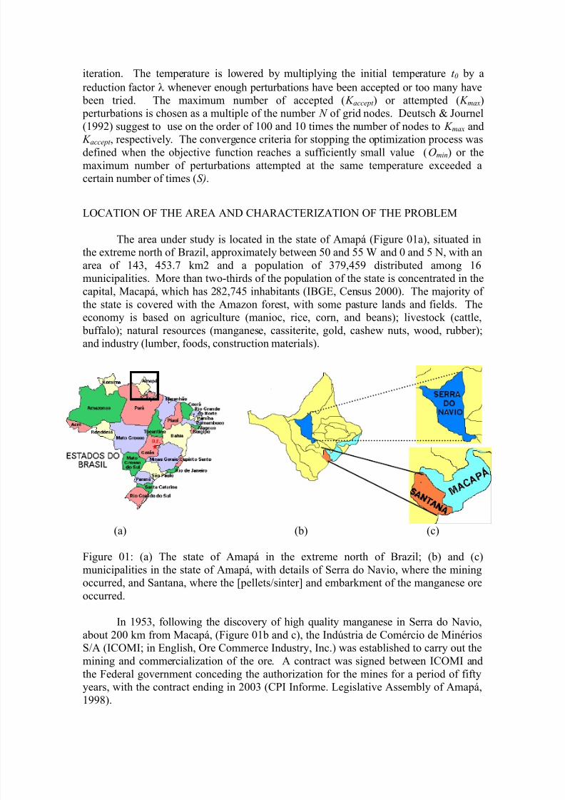
The area under study is located in the state of Amapá (Figure 01a), situated inthe extreme north of Brazil, approximately between 50 and 55 W and 0 and 5 N, with anarea of 143, 453.7 km2 and a population of 379,459 distributed among 16
municipalities. More than two-thirds of the population of the state is concentrated in thecapital, Macapá, which has 282,745 inhabitants (IBGE, Census 2000). The majority ofthe state is covered with the Amazon forest, with some pasture lands and fields. Theeconomy is based on agriculture (manioc, rice, corn, and beans); livestock (cattle,
buffalo); natural resources (manganese, cassiterite, gold, cashew nuts, wood, rubber);and industry (lumber, foods, construction materials).
(a) (b) (c)
Figure 01: (a) The state of Amapá in the extreme north of Brazil; (b) and (c)municipalities in the state of Amapá, with details of Serra do Navio, where the miningoccurred, and Santana, where the [pellets/sinter] and embarkment of the manganese oreoccurred.
In 1953, following the discovery of high quality manganese in Serra do Navio,about 200 km from Macapá, (Figure 01b and c), the Indústria de Comércio de MinériosS/A (ICOMI; in English, Ore Commerce Industry, Inc.) was established to carry out themining and commercialization of the ore. A contract was signed between ICOMI andthe Federal government conceding the authorization for the mines for a period of fiftyyears, with the contract ending in 2003 (CPI Informe. Legislative Assembly of Amapá,
In order to carry out the mining, ICOMI constructed, in addition to the industrialinstallation, a residential community near the manganese mines in Serra do Navio withcomplete infrastructure including sanitation, leisure, schools, a supermarket, hospital,and housing for the company’s employees and their families. A railroad was also builtwhich linked the village of Serra do Navio to an industrial area on the banks of the north
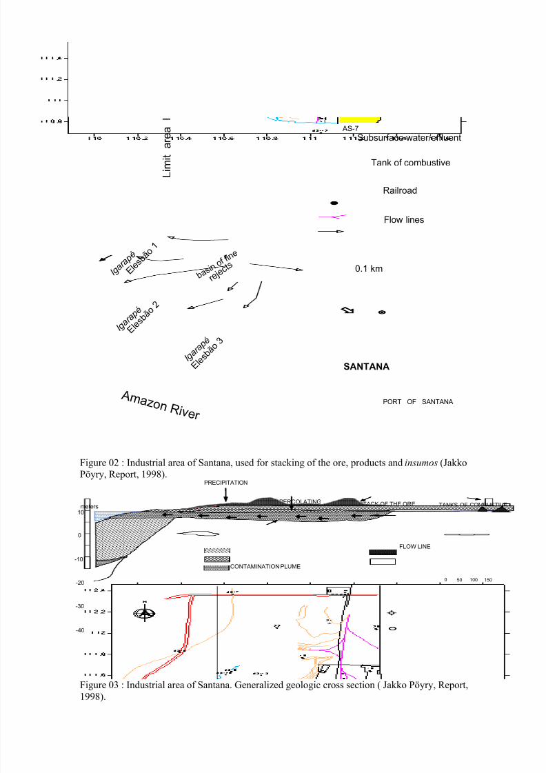
canal of the Amazon River, in the municipality of Santana (Figure 01b and c), about 30km from Macapá, from where the sold manganese was shipped. This approximately129 hectare area (Figure 02), characterized as being strictly for industrial use, was used
basically to stock the ore (manganese and iron), products (pellets/sinter and alloys) andraw materials (fuel, coke, etc.) that arrived and departed via this ICOMI port and railterminal (JAAKKO POYRY ENGENHARIA, 1998 report). The manganese andcromite ore were thus transported by railroad from the mines in Serra do Navio to theICOMI industrial area in the Port of Santana, a distance of approximately 200 km.
Figure 03 presents a schematic geological section of the eastern sector of theICOMI area where various units and stockpiles are concentrated. It was observed that
the geological profile at the banks of the Amazon River present the following sequencefrom the top to the base: alluviums (silty organic clay) extending approximately 150mand measuring up to 40m in thickness; horizon of clay silts (superior/upper horizon)with a continuous thickness around 6 to 8m and a horizon of hard clays (inferior/lowerhorizon). The area of interest, which extrapolates the perimeter of ICOMI, sits atopsediments of the Barriers Formation, constituted of silty organic clays, clay silts, andhard clay with scarce intercalations of fine and coarse sand. The water level (WL) thatseparates the non-saturated horizon (above the WL) from the saturated (below the WL)varies in depth, ranging from a few centimeters near the riverbank up to a maximumvalue around 9.0m in the northern portion. These depths oscillate throughout the yeardue to the seasonal variations in the potenciometric surface of the underground water.The potenciometric surfaces, measured in the wells that were installed, condition themovement of the water underground (subterranean flow). Thus, for the informationobtained in June and August, 1997, it was observed that the subterranean flow developsfrom the center of the area, the region between wells 16 and 21, flowing radially indirection of the Amazon River and other neighboring areas (JAAKKO POYRYENGENHARIA, 1998 report).
After extracting 60 of the estimated 65 million tons of manganese ore reserve inSerra do Navio, ICOMI presented, in November of 1997, a report to demonstrate theexhaustion of the deposit. There are strong indications of a series of environmental
problems caused by the mining of the manganese deposits in Amapá. A ParliamentaryCommission of Inquiry established in April, 1999, to investigate the dismantling process of ICOMI presented documents (JAAKKO POYRY ENGENHARIA, 1998report) about the environmental situation in the industrial area of Santana, denouncingthat the quality of the surface and underground water had been affected, mainly due tothe residue deposits generated in the manganese ore pellets/sinter plant in the area.Regarding the potential for contamination, Arsenic and Manganese were found to be
present in levels exceeding standards established by the brazilian law in the surface andunderground water linked to the fine residues stocked in the Refuse Basin and vicinity.The standards are established in accordance with the World Health Organization(WHO), which considers water containing more than 0.05 ppm of arsenic inappropriate
for human consumption. However, the Environmental Protection Agency (EPA) isconcluding regulations to reduce the risks to public health of arsenic in drinking water.
The EPA is establishing a new standard of 10 parts per billion (ppb) for arsenic indrinking water to protect consumers against long term effects of chronic exposure toarsenic in drinking water. Such effects include cancer and other health problemsincluding cardiovascular disturbances, diabetes, as well as neurological effects (EPA,2001).
To represent the area under study, fifty locations were selected corresponding to37 monitoring wells and 13 samples of sub-surface/effluent water (Figure 02) whereanalysis of the contaminants (manganese, arsenic, and iron) was carried out. The
physical-chemical analyses of soil and water samples and the characterization ofresidues were conducted by the S.G.S. laboratories of Brazil and CEIMIC AvaliaçãoAmbientais S/C Ltda.(in English, Environmental Evaluation, Ltd.), selected based ontheir technical qualifications, equipment used, and recognition of their services(JAAKKO POYRY ENGENHARIA, 1998 report).
RESULTS AND DISCUSSION
Data and Statistical Description
Table 01 and Figure 04 (frequency distribution, right column), show that thearsenic, manganese and iron variables have highly asymmetric distributions, indicatingthe presence of a few large concentrations. The metal concentrations are expressed in
parts per million (ppm). The manganese concentration showed the highest asymmetry(6,71), probably due to the occurrence of a single high value concentration (216 ppm).In Figure 04 (cumulative frequency distributions, right column), the vertical dashedlines indicate, for each metal, the tolerable maxima for water, as defined by the
brazilian law; see Table 01 for exact values. The percentage of data exceeding thesecritical thresholds is given at the top of each graphic. These proportions are larger formanganese (58%) followed by iron (34%) and arsenic(22%). The gray scale maps inFig. 04 (left column) provide a preliminary description of the extension of thecontamination by the metals in study. The highest arsenic and manganeseaccumulations are located in the central and southern region. The highest ironaccumulations are located in the southeast region of the study area. Contour maps would
be prepared from these data to characterize the site . The boundaries betweencontaminated and uncontaminated zones would be identified by the location of thesecontours.
Table 02 gives the correlation coefficients among the variables. The correlationcoefficient of Pearson, , provides a measure only of linear relation between twovariables and is complemented by rank correlation coefficient, rank , which considersthe ranks of the data. Unlike the traditional correlation coefficient, the rank correlationcoefficient is not strongly influenced by extreme pairs. Large differences between thetwo reflects either a nonlinear relation between the two variables or the presence of
pairs of extreme values. The results show a significant relationship between arsenic andmanganese concentrations. Larger manganese concentrations tend to be associated withlarger concentrations of arsenic. Both measures, and rank , are similar, as arsenic vs.manganese as manganese vs. iron, which indicates that extreme values do not greatlyaffect the linear correlation coefficients. The sample does not show any sign of an
association between arsenic and iron concentrations.
Table 02. Correlation coefficient of Pearson ( ) and Rank correlation coefficient ( rank )Variables prob t rank prob t
Arsenic vs Iron
Arsenic vs Manganese
Iron vs Manganese
0,028
0,434
0,274
0,847 ns
0,002 ***
0,054 ns
-0,104
0,455
0,235
0,4709 ns
0,0009 ***
0,1001 ns
ns : not significant*** 1% significant
Sample semivariograms and spatial continuity model
Sample semivariograms were computed using the semivariogram estimator presented in Deustch & Journel, 1992. Because the sample size was small, it was not possible to calculate informative directional sample semivariograms. For this reason, thecorrelation structure of the variables was considered isotropic, and "omnidirectional"sample semivariograms were computed (Isaaks e Srivastava, 1989). To the variablesstudied, spherical semivariograms models were fit defined by:
ahif c
ahif a
h
a
h
ch
,5.05.1.)(
3
(3)
where h is the separation distance, c is the sample variance and a is the range orcorrelation length. The sample semivariograms and models to each variable are shownin Figure 5 and in the Table 03 the model parameters are presented. The iron presentedthe best spatial correlation, indicated by smaller nugget effect and arsenic showed thelargest spatial continuity, due to having the largest range.
Table 03. Summary of fitted semivariogram model parametersVariable Nugget, C 0 Sill, C Range, a (km)ArsenicManganeseIron
0.250.270.04
0.850.750.92
0.320.180.20
Simulations
We used the programs from the GSLIB library (Deustch & Journel, 1992). Fiftyconditional simulations of the contaminant concentrations were generated on a regular35 x 50 grid using the simulated annealing algorithm (Sasim). Figure 06 shows for allvariables, the first realization and fitted semivariograms for the five initial realizations.Edge effects may occur by annealing simulation when the univariate distribution ishighly skewed. These effects can be avoided by weighting the border pairs (Deustch &Cockerham, 1994) or, alternatively, by a combination of reducing the number of lagvectors used in the objective function, positioning the lag vectors according to
anisotropy of the spatial variability model, and supplying a more advanced, realisticinitial configuration (Carle, 1997). The edge effects were noticeable in the manganesevariable that presented the largest asymmetry. In this case, we used the alternative
procedure of reducing the number of lags vectors (4 lags) of the objective function andrealistic initial configuration. One can observe a decreasing of the border effects and inthe quality of fitted semivariograms (Figure 06, middle graphics). However, the fittedsemivariograms of the studied variables can be considered acceptable. Probabilisticsummaries of the simulations were obtained using the computer program Postsim. Amap is presented of the expected value estimates (E-type) that were obtained byaveraging the 50 simulated values for each realization. E-type estimate maps andrespective histograms of each variable are presented in Figure 07. The areas withhigher levels of arsenic contamination are located in and around the fine refuse basin,while manganese occupied a much larger section, covering almost the entire study area,including a small portion outside the industrial area. Iron concentrations are higher in asoutheast portion of industrial areas. Maps showing the probability of exceeding a
particular threshold were computed from the set of simulations by counting the numberof corresponding pixels across the set of sthocastic images that exceed the statedthreshold, converting the sum to a proportion, and presenting the spatially empirical
probability in map form. Figure 08 ( on the left)shows the probability maps of eachvariable considering as cutoff the tolerable maxima of 0.05, 0.1 and 0.3 ppm to arsenic,manganese and iron, respectively. These maps confirmed that manganese is responsible
for the largest contamination in the study area. Iron and arsenic occur at largercontamination levels located in small areas. Figure 8 (on the right) shows the estimatesof the contamination in the area for the several probability levels, related to the tolerablemaxima allowed for each variable. The portion of the area classified as contaminated isrelatively insensitive to the choice of a probability cutoff until it reaches about 0.5 foriron and manganese and 0.2 for arsenic.
CONCLUSIONS
In this paper the annealing simulation was used to carry out a probabilistic
evaluation of arsenic, manganese and iron contamination in the port of Santana, Amapa,Brazil. The probabilistic approach explicitly recognizes the uncertainty in contaminant
concentrations at unsampled locations. Therefore, the area and boundaries ofcontaminated zones are uncertain. Specific values of these quantities can be obtainedthrough the specification of a target probability or level of risk. The site is discretizedinto an array of blocks with known size and shape, and a simulated value ofcontaminant concentration obtained for each block. Fifty realizations were generated of
the contaminant concentrations where all matched reasonably to the same statistics(histogram, semivariogram) allowing the assessment of the uncertainty about thespatial distribution of the contaminants. The choice of the probability cutoff wasdetermined by tolerable maxima established by the government agency, however othercriteria can be used as the established by searchers, regulatory agencies, etc. Thesimulated maps can be used as input into transfer functions, as health and remediationcosts.
REFERENCES
Carle, S.F., 1997, Implementation schemes for avoiding artifact discontinuities insimulated annealing: Mathematical Geology, v. 29, n. 2, p. 231-244
CPI - Comissão Parlamentar de Inquérito Informe, maio/98, Assembléia Legislativa doEstado do Amapá. no.01, Macapá-AP, Brazil.
Deustch, C. and Cockerham, P., 1994, Practical considerations in the application ofsimulated annealing to stochastic simulation: Mathematical Geology, Vol. 26, n0. 1, p.67-82
Deustch, C. and Journel, A. G., 1991, The application of simulated annealing to
stacastic reservoir modeling: Soc. Petroleum Engineering, SPE Paper 23565, 30 p.
Deustch, C. V., and Journel, A. G., 1992, GSLIB: Geostastical Software Library anduser's guide: Oxford Univ. Press, New York, 340 p.
Dougherty, D. E., and Marryott, R. A., 1991, Optimal Groundwater Management, 1.Simulated annealing: Water Resources Research, vol. 27, n0. 10, p. 2491-2508.
Environmental Protection Agency, January 2001, Drinking water standard for arsenic :Office of Water, 4606, www.epa.gov/water .
Fang, J. H. and Wang, P. P., 1997, Random field generation using simulated annealingvs. fractal-based stochastic interpolation: Mathemati-cal Geology, v. 29, n. 6, p. 849-858
Geman, S., and Geman, D., 1984, Stochastic relaxation, Gibbs distributions. And theBayesian restoration of images: IEEE Trans Pattern Anal. Machine Intell. PAM1. V.6no. 6, p.721-741
Goovaerts, P., 1977a, Kriging vs. stochastic simulation in soil contamination in Soares,A., Gómez-Hernadez, J., and Froidevaux, R., eds. GeoENV I-Geostatistics forenvironmental applications: Kluwer Acadaemic Publ. Dordrecht, p. 247-258
Goovaerts, P., 1997, Geostatistics for Natural Resources Evaluation. Oxford Univ.Press, New York, 483 p.
Goovaerts, P., 1998, Accounting for estimation optimality oriteria in simulatedannealing: Mathematical Geology, Vol. 3, n0. 5, p. 511-534
Gupta-Datta, A., Larry, W.L. and Pope, G.A., 1995, Characterizing hetero-geneuos permeable media with spatial statistics and tracer data using se-quencial simulatedannealing: Mathematical Geology, v. 27, n. 6, p. 763-787
IBGE - Instituto Brasileiro de Geografia e Estatística, Brazil, Censo 2000.
Isaaks, E. H., and Srivastava, R. M., 1989, Applied Geostatistics. Oxford UniversityPress, New Yprk, NY, 561 pp.
Journel, A. G., and Alabert, F., 1990, New method for reservoir mapping: Jour. of
Petroleum Technology, p. 212-218
Marryott, R., Dougherty, D. E., and Stollar, R. L., 1993, Optimal Ground-waterManagement, 2. Applications of simulated annealing to a field-scale contamination site:Water Resources Research, vol. 29, n0. 4, p. 847-860.
Relatório JAAKKO PÖYRY ENGENHARIA, Maio/98, Disposição final dos resÍduosda usina de pelotizacao/sinterizacão estocados na área industrial da ICOMI/Santana,AP. Santana, Amapá, Brazil, 66 p.
Zheng, C. and Wang, P. P., 1996, Parameter structure identification using tabu searchand simulated annealing: Adv. Water Res., v. 19, no. 4, p. 215-224
Figure 04. Data locations, histograms and cumulative distribuitions of metal concentrations,
arsênic (top), manganese ( middle ) and iron ( bottom ). The proportions of data that exceed thetolerable maxima is represented by the vertical dashed lines.
Figure 05. Experimental omnidirectional semivariograms for Arsenic (top), Manganese(middle) and Iron (bottom). The solid line represents the fitted model.
Figure 06. Conditional Annealing realizations of arsenic (top), manganese (middle) and Iron
(bottom) concentrations in ppm (left column). Experimental semivariograms (black lines) forthe five initial realizations and the model semivariogram (blue lines) are show on right column.
Figure 07. "E-type" estimate maps of arsenic (top), manganese (middle) and Iron (bottom)concentrations in ppm (left column) derived from postprocessing 50 simulations and respectivehistograms (right column).


![Geophysical Contribution for the Mapping the Contaminant ...[14,15,16,17,18,19], and [20]. Moreover, the uncertainty of geophysical interpretation can be notably reduced when several](https://static.documents.pub/doc/80x56/606b6f293136ad1de72f87b1/geophysical-contribution-for-the-mapping-the-contaminant-141516171819.jpg)


![Air Contaminant _54.12_ [Preamb]](https://static.documents.pub/doc/80x56/5695cf481a28ab9b028d6988/air-contaminant-5412-preamb.jpg)


