WATER RESOURCES RESEARCH, VOL. 25, NO.6, PAGES 1141-1148, JUNE 1989

~,0Contaminant Transport and Biodegradation

A Numerical Model for Reactive Transport in Porous Media

MICHAEL A. CELIA

,

Department of Civil Engineering, Massachusetts Institute of Technology, Cambridge

,

J. SCOTT KINDRED

Golder

Associates Inc., Redmond, Washington

ISMAEL HERRERA

lnstituto de Geofisica, National Autonomous University of Mexico, Mexico City

A new numerical solution procedure is presented for simulation of reactive transport in porousmedia. The new procedure, which is referred to as an optimal test function (OTF) method, isformulated so that it systematically adapts to the changing character of the governing partialdifferential equation. Relative importance of diffusion, advection, and reaction are directly incorpo-rated into the numerical approximation by judicious choice of the test, or weight, function that appearsin the weak form of the equation. Specific algorithms are presented to solve a general class ofnonlinear, multispecies transport equations. This includes a variety of models of subsurface contam-inant transport with biodegradation.

The recent work of Herrera [1984, 1985a, b], Herrera etal. [1985], and Celia et al. [1989a] provides a systematicframework in which numerical solutions to general second-order equations can be obtained. The procedure leads tonumerical approximations that automatically change as thegoverning partial differential equation changes. This isachieved by choosing test functions, which are present in aweak form of the original governing equation, to satisfyspecific, rigorously derived criteria. No arbitrary parametersare involved. It is the purpose of this paper to develop asolution algorithm, based on this procedure, for systems ofadvective-ditIusive-reactive transport equations. In a com-panion paper [Kindred and Celia, this issue] the methodol-ogy is applied to a specific model of transport in biologicallyreactive porous media.

The presentation in this paper begins by exposing theunderlying numerical algorithm for the case of a singleadvective-ditIusive-reactive transport equation with con-stant coefficients. This allows the salient features of themethod to be explained in a simple mathematical setting.The procedure is then extended to the case of spatiallyvariable coefficients, and finally to the case of multipleequations that are coupled through nonlinear reaction terms.Example calculations are presented to demonstrate thenumerical procedure and to provide a direct link to thebiodegradation model that is developed in the companionpaper [Kindred and Celia, this issue].

1. INTRODUCTION

A proper description of contaminant transport is impor-tant in many aqueous systems. For subsurface flows, de-scription of the flow physics must often be augmented bychemical and/or biological considerations. This generallyleads to advective-di1Iusive-reactive transport equations.When multiple species are present in the aqueous phase, thegoverning equations form a set of partial differential equa-tions that are coupled through reaction terms. These equa-tions generally need to be solved numerically.

The transport equation is one for which numerical solutionprocedures continue to exhibit significant limitations forcertain problems of physical interest. The most widely citedexample is the case of advection domination. In this case,one is usually forced to choose between nonphysical oscil-lations or excessive (numerical) diffusion. While a variety ofmethods have been developed specifically for advection-dominated flows [Leonard, 1979; Hughes and Brooks, 1982;Tezduyar and Ganjoo, 1986; Baptista, 1987], only partialsuccess can be reported to date.

A key to providing reliable numerical simulations is rec-ognition of the changing nature of the governing equation.Diffusion domination implies behavior analogous to thatpredicted by model parabolic partial differential equations;advection domination implies behavior analogous to first-order hyperbolic partial differential equations; and reactiondomination implies first-order ordinary differential equation(in time) behavior. A numerical procedure that fails toaccommodate these disparate behaviors cannot be expectedto produce reliable numerical solutions.

f

NUMERICAL ALGORITHM-SINGLE SPECIES

TRANSPORT WITH CONSTANT COEFFICIENTSCopyright 1989 by the American Geophysical Union.

Paper number 89WRO0271.0043-1397/89/89WR-00271 $05 .00

The numerical development begins by examining a singlespecies, advective-difIusive-reactive transport equation

1141

1142 CELIA ETAL.: CONTAMINANT TRANSPORT AND BIODEGRADATION, 1

The first key to the numerical procedure is application ofintegration by parts twice to each term of the summation in(4). For each element integration, the first integration byparts produces

R au/at + v au/ax -D a2u/ax2 + Ku = f(x, t) (1)

O~x~L t>O

i~j+I(:£xU)W(X) dx

= (Xj+ I

JXj

a2u au )D -;;::z -V --Ku w dx =ax ax

auD-w- Vuw

ax

r

au dw dw )-D--+ Vu--Kuw dxaxdx dx

+ (XI + I I

JX} \ /

Application of an additional integration by parts then yields

L X}+I [ au dw (:£ u)w dx = D -w -Du --Vuw

x ax dx

x) -

+ (Xj+ I

JXj

dw

dx -KW)UdX

d2wDp+V

u(O, t) = go t > 0

au/ax(L, t) = gL t > 0

u(x, 0) = uo(x) 0 ~ x ~ L

defined over the finite spatial domain n = [0, L]. Anyboundary conditions can be accommodated in the numericalalgorithm; the conditions given above provide a typicalexample. Nomenclature is such that R is a retardationcoefficient (dimensionless); V is fluid velocity (L/1); D is adiffusion coefficient (L 2/1); K is a first-order reaction coeffi-cient (1/1); f is a given forcing function; and u(x, t) is thedependent scalar of interest, which in this case is a measureof concentration of a dissolved substance. The forcingfunction f(x, t) is a source/sink term that may includereaction terms that are not dependent on the unknownfunction u. To begin the numerical development, let thecoefficients R, V, D, and K be assumed constant. Thenumerical procedure that is to be applied to (1) consists ofapplication of the algebraic theory of Herrera [1984, 1985a,b] in space, thereby producing a semidiscrete system ofordinary differential equations in time. This resulting set ofordinary differential equations is then integrated in timeusing standard methods.

Let (1) be rewritten in the form

:£xu = D a2u/ax2 -V au/ax -Ku = R au/at -f(x, t) (2)

where the operator :£x incorporates both the spatial deriva-tives and the reaction term. The weak form of (2) is thenformed by multiplying the equation by a weight, or test,function, w(x), and integrating over the domain [0, L]

-L

(D a2u/ax2 -V au/ax -Ku)w(x) dx

[ au dw ]XJ+l LXJ+' = D a; w -Du ~ -Vuw + (:;E~w)u dx (5)

XJ Xl

where :;Ex is the original spatial operator and :;E': is its formaladjoint.

The second key to the numerical procedure is to recognizethat the original integral (on the left side) of (5) can bereplaced by nodal evaluations by choosing w(x) such that:;E*xw = 0 within each [xi' xi+I]' That is to say, proper choiceof the test function w(x) effectively concentrates informationat node points and eliminates interior element integrations.In addition, the concentration of information at node pointsis accomplished in the absence of any trial function definition(as would be the case in a standard finite element formula-tion). Both the special choice of test function and the lack ofa trial function distinguish this numerical formulation fromstandard finite element or Petrov-Galerkin methods.

Consider a choice of w(x) that satisfies :;E*xw = 0 withineach [xi' xi+I],j=O, 1, ..., £-1. Furthermore, allow w(x) theability to exhibit discontinuities at node points. Given such adefinition ofw(x), (4) and (5) can be combined and restated interms of known coefficients and unknown nodal values of thedependent variable. In light of (5) and the fact that :;E*xw = 0,(4) can be rewritten as

Eil (Xj'j = 0 J x)

(:£xu)w dx

= iL(R au/at -f)w(x) dx (3)

Next, let the spatial domain [0, L] be subdivided into Esubintervals {[XO, XI]' [XI' X2]' ..., [XE-I' XE]}' with Xo = 0,XE = L. These subintervals, or elements, are separated bythe E + 1 node points {XO, XI' ..., XE}' If the solution u isassumed to be at least (:;1 continuous, u E (:;1[0, L](that is, uand au/ax are continuous functions over Os X s L), and w(x)is at least (:;-1 continuous, wE (:;-1 [0, L] (that is, J~ w(x')dx' is a continuous function over 0 ~ X ~ L), then theintegral on the left side of (3) can be written equivalently as

iL(D a2u/axZ -V au/ax -Ku)w(x) dx

E-)

= Lj= )

auUJ" -[[Dw ]1-;- j

} uX

dwD ~ + Vw

£-1

= j~O i:j+l(D iJ2U/iJx2 -V iJu/iJx -Ku)w(x) dx (4)

+[(-D~

) au ]L -Vw u + Dw -(6)

ax 0

In (6), the double bracket denotes a jump operator, which isdefined by [[o]]x = lim.,--.o [(o)x+e-(o)x-e]. Since D, V, and

J J J

The equality (4), which introduces elementwise integration,is permissible due to the continuity constraints on u and w.The case of lower continuity on u has been treated byHerrera [1984, 1985a, b]; for the present development, u E1[1 will suffice. Also, let any discontinuities that occur in w(x)be restricted to node points. Within each [Xp Xj+I]' it isassumed that w(x) E 1[2.

1143CELIA ET AL.: CONTAMINANT TRANSPORT AND BIODEGRADATION, 1

ware are all known, the only unknowns in (6) are the 2£ +2 nodal values {Uj, (iJu/iJx)j}.f~o' These nodal values corre-spond to the function U and its spatial derivative. Thesevalues are unique at each node by the continuity assumptionU E C1[O, L]. Equation (6) can be written more succinctly asa simple linear combination of known coefficients and un-known nodal values

boundary conditions, 2E+2linear algebraic equations resultfor the 2E+2 nodal unknowns. Solution of this set ofequations produces exact nodal values, since no approxima-tion has been introduced, and the set of test functions is Tcomplete [see Herrera, 1984]. Detailed algorithms for thecase of constant coefficient, ordinary differential equationsare presented by Herrera et al. [1985].

When au/at e~ 0, the time dimension must be included.Examination of (3) indicates that a spatial integral of theproduct of (au/at)(x,t) and w(x) must be evaluated. Toperform this integration, au/at is approximated using apolynomial expansion that involves the nodal values appear-ing in the expression on the right side of (6). The naturalchoice for the approximation developed above is a piecewisecubic Hermite polynomial interpolation in space, since thisinvolves nodal values of u and au/ax, namely,

i L E au(:£xu)w dx = 2: Ajuj + Bj a;j (6')

0 j=O

For the operator :£x of (2), the formal adjoint operator is,,ccording to (5),

:£1 = Dd2/dx2 + Vd/dx K (7)

The homogeneous solutions corresponding to :£; are givenby E

iJu/iJt = iJu/iJt = L {Vj(t)c/Joj(x) + (iJ V/iJx)J{t) <P\j (x)} (10)j=O

In (10), {Vi' (iJV/iJx)i}f~o are time-dependent nodal values offunction and spatial derivative, and <Poi, <P1j are standardcubic Hermite polynomials (see, for example, Carey andaden [1983, pp. 63-65]). Substitution of expansion (10) intothe integral of interest yields

'l'\(x) = exp [(a + /3)x] (8a)

'l'2(X) = exp [(a -/3)x] (8b)

where a = -VIW and /3 = (1/2D) (V2 + 4KD)I/2. Equations(8a) and (8b) represent the two fundamental solutions of thehomogeneous adjoint equation. Any linear combination ofthese solutions also satisfies the homogeneous adjoint equa-tion. The computational procedure proposed herein uses astest fullctions two nonzero solutions to ':£:W = 0 defined in

each element and formed as linear combinations of solutions(8a) and (8b). These functions are defined such that they arenonzero only within the element of interest, and zero in allother elements. As such, each w(x) E (:-1[0, L]. For anyelement e, defined by [xi' Xj+1]' the test functions are definedby

d [ iJUj ] (L }+ di -;;:;- (1) Jo cf>ij(X)w(X) dx (11)

Given that cPoj{X), cPv{x), and w(x) are each well defined andknown functions, the integrals can be evaluated directly and(11) can be written, with inclusion of the coefficient R, as

w1(x) = C11 exp [(a + f3)x) + C12 exp [(a -f3)x) (9a)

Xi<X<Xi+

R (II'wj(x) = 0 x < Xj X> Xj +

wz(X) = C21 exp [(a + f3)x] + C22 exp [(a -f3)x]

~)ax

(9b) Thus the resulting approximation that derives from (11), (6),and (3) is

X'<X<Xj+

J

E { d d ( aUo) dUo}" ao-(U)+ ,B °- -1 -AoUo-Bo-1L., :I dt J :/ dt ax :I J J axj=O

w~(x)=O X<Xj x>Xj+1

The constants CII, C12' C21' and C22, are chosen, forconvenience, to satisfy the conditions w~(x) = 1, W~(Xj+J =0, W2(X) = 0, and W2(Xj+J = 1. Therefore CII = -exp[-(a+ f3)xj-2f3(llx)]/{1-exp [-2f3(llx)]}, C 12 = exp[-(a-f3)xj]/{l-exp [-2f3(llx)]}, C21 = -exp[-(a-f3)xj+I-2f3x)/{1-exp [2f3(llx)]}, and C22 = exp[-(a-f3)xj+J/{l-exp [2f3(1lx)]), with Ilx = Xj+I-Xj' Anyother linear combination of the fundamental solutions (8)would be equally acceptable. Since there are E elements, 2Eequations are produced corresponding to the 2E linearlyindependent test functions, {w~(x), W2(X)}:=I' The undeter-mined nodal values that appear in (5) are the function u andthe spatial derivative au/ax, forming the set of 2E+2 un-knowns {Uj, (au/ax)j}f~o' Two boundary conditions providethe two additional equations needed to close the system.

For steady state conditions, au/at = 0 and (1) reduces to anordinary differential equation. After evaluation of the rightside forcing term I~x)w(x) dx and imposition of the two

=iL.f(x, t)w(x) dx (12)

An equation of the form of(12) is written for each of the 2£choices of w(x) given in (9). The two boundary conditionsrequired for the second-order equation (I) provide twoadditional equations, so that 2£+2 equations result for the2£+2 nodal values. This provides the semidiscrete system ofequations

P .dU/dt -Q .U = F (13)

where matrix P contains the ap f3j coefficients of (11), Qcontains the coefficients Aj, Bj of (6), and the vector Ucontains nodal values of U and au/ax. The structure of thecoefficient matrices P and Q is exactly analogous to that ofstandard cubic Hermite collocation. This structure is illus-

1144 CELIA ET AL.: CONTAMINANT TRANSPORT AND BIODEGRADATION, I

p=

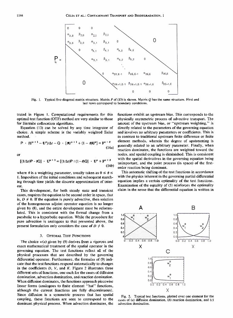
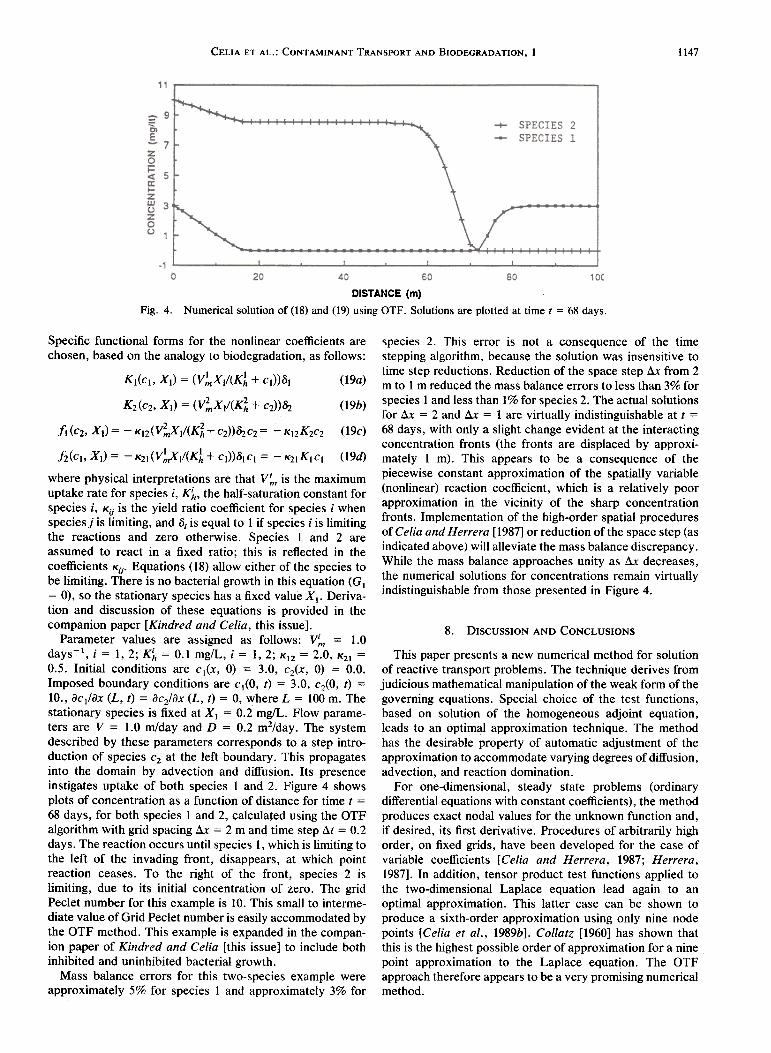
Fig.

1. Typical five-diagonal matrix structure. Matrix P of (13) is shown. Matrix Q has the same structure. First andlast rows correspond to boundary conditions.

trated in Figure 1. Computational requirements for thisoptimal test function (OTF) method are very similar to thosefor Hermite collocation algorithms.

Equation (13) can be solved by any time integrator ofchoice. A simple scheme is the variably weighted Eulermethod.

p. (un+l-un)/llt-Q. [8Un+l+(1-8)un]=Fn+6(14a)

= [(II Ilt)P+(l- 8)Q] .Un + Fn + 6

(14b)

or[(l/~t)P-IJQ] .Un + I

where 8 is a weighting parameter, usually taken as 0 :5 8 :5I. Imposition of the initial conditions and subsequent march-ing through time yields the discrete approximation of inter-est.

This development, for both steady state and transientcases, requires the equation to be second order in space, thatis, D # O. If the equation is purely advective, then solutionof the homogeneous adjoint operator equation is no longergiven by (8), and the entire deyelopment must be reformu-lated. This is consistent with the formal change from aparabolic to a hyperbolic equation. While the procedure forpure advection is analogous to that presented above, thepresent formulation only considers the case of D # O.

A"o

r0.6 0.6

0.40.2

nl

e eXW1 w2 J

jJJ

0.4 (J.tS O.a 1.0

X

3. OPTIMAL TEST FUNCTIONS

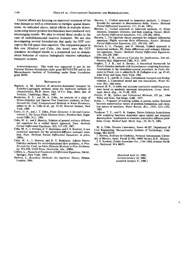
The choice w(x) given by (9) derives from a rigorous andexact mathematical treatment of the spatial operator in thegoverning equation. The test functions reflect all of thephysical processes that are described by the governingdifferential operator. Furthermore, the formulas of (9) indi-cate that the test functions respond automatically to changesin the coefficients D, Y, and K. Figure 2 illustrates threedifferent sets offunctions, one each for the cases of diffusiondomination, advection domination, and reaction domination.When diffusion dominates, the functions approach piecewiselinear forms (analogous to finite element "hat" functions,although the current functions are fully discontinuous).Since diffusion is a symmetric process that has spatialcoupling, these functions are seen to correspond to thedominant physical process. When advection dominates, the

Fig. 2. Typical test functions, plotted over one element for thecases of (a) diffusion domination, (b) reaction domination, and (c)advection domination.

functions exhibit an upstream bias. This corresponds to thephysically asymmetric process of advective transport. Theamount of the upstream bias, or "upstream weighting," isdirectly related to the parameters of the governing equationand involves no arbitrary parameters or coefficients. This isin contrast to traditional upstream finite difference or finiteelement methods, wherein the degree of up streaming isgenerally related to an arbitrary parameter. Finally, whenreaction dominates, the functions are weighted toward thenodes, and spatial coupling is diminished. This is consistentwith the spatial derivatives in the governing equation beingunimportant, and the point process (in space) of the first-order reaction being dominant.

This automatic shifting of the test functions in accordancewith the physics inherent in the governing partial differentialequation implies a certain optimality of the test functions.Examination of the equality of (5) reinforces the optimalityclaim in the sense that the differential equation is written in

CELIA ET AL.: CONTAMINANT TRANSPORT AND BIODEGRADATION. I 1145

terms of nodal values in a mathematically precise way.Furthermore, optimal accuracy occurs for steady state equa-tions in both one dimension (exact nodal solutions forequation (1) when R = 0) and two dimensions (see Discus-sion in section 8). The numerical algorithm presented aboveis therefore referred to as an OTF method.

equation of the form of (1), where the coefficients arefunctions of the unknown u, linearization involves evalua-tion of the coefficients using previous (known) values of thesolution. These can be values of previous iterations or valuesat previous time steps. In either case, the linearized govern-ing equation is analogous to a variable coefficient problem.Techniques discussed in the previous section therefore per-tain.

Linearization can take one of several forms. For timemarching problems, nonlinear coefficients can be estimatedfrom solutions at previous time steps, allowing for solutionat the new time level exclusive of iteration. Conversely,progressively improved solutions at the new time level canbe obtained through iterative solution procedures. Theseiterative procedures include simple (Picard) iteration, New-ton-Raphson iteration, and various modifications of each.The linearization that is chosen herein for the case ofnonlinear reactive transport uses a noniterative time march-ing algorithm coupled with a second-order projection tech-nique for estimating the nonlinear coefficients. Estimates ofnonlinear coefficients are based on solutions at the previoustwo time levels. For a time weighting parameter 8, as used in(14), the appropriate projected value is given by

un+8=(1+8)un-8un-l (15)

This is a second-order (in time) estimate for Un+B. This verysimple linearization was chosen because of the relativelymild nonlinearities and the very good numerical results thatwere subsequently produced. As stated previously, applica-tion of the optimal test function method is indifferent to thelinearization chosen; OTF is applicable to any linearizationprocedure.

4. TREATMENT OF NONCONSTANT COEFFICIENTS

When the coefficients in (1) exhibit spatial variability, it isgenerally not possible to exactly satisfy the homogeneousadjoint equation, ~:w = O. In this case, an approximation

procedure is required to provide good estimates to w, so that~:w = O.

Two approaches have been developed to treat the variablecoefficient case. The first, which is used herein, involvesreplacement of the coefficients in (1) with piecewise La-grange polynomials. The approximate coefficients have dif-ferent polynomial definitions in each element and are gener-ally discontinuous across element boundaries. The basicidea is that with these approximate coefficients, the adjointequation is simply an ordinary differential equation withpolynomial coefficients. As such, two independent seriessolutions can be developed for the homogeneous adjointequation using standard techniques (see, for example, Hilde-brand [1976]). Celia and Herrera [1987] have shown thatthrough judicious choice of interpolation points within eachelement, piecewise nth degree Lagrange interpolants canprovide O«l1xfn+2) accuracy in the numerical solution. Thearguments used to develop this theory are analogous to thoseused to choose collocation point locations in the collocationfinite element method (see, for example, Prenter [1975]). Theinterpolation points in the OTF method, and the collocationpoints in the collocation finite element method, both turn outto be the Gauss-Legendre integration points within eachelement [Celia and Herrera, 1987]. An alternative approachfor developing test functions uses a local (elementwise)collocation solution for the homogeneous adjoint equation.This again yields two independent solutions for w(x) withineach element. Details of this local collocation procedure areprovided by Herrera [1987].

For the current treatment, consider approximation of thecoefficients by piecewise constants. That is, the coefficientsare constant within each element and can change from oneelement to the next. Since ~:w = 0 within each element

separately, the adjoint equation in any element involvesconstant coefficients. Therefore si~ple analytical solutionscan be obtained for the test functions. By the error estimatecited above, this provides O«l1xf) accuracy in the approxi-mation. If D(x), V(x), and K(x) are replaced by D(x), V(x),and R(x), with overbarred quantities referring to piecewiseconstant approximations, then the test functions remain asdefined in (9) with D, V, and K, interpreted to be the valueswithin the element of interest.

6. SETS OF COUPLED EQUATIONS-REACTIVETRANSPORT OF MULTIPLE SPECIES

Mathematical description of transport of multiple speciesin flowing groundwater involves a set of coupled, advective-diffusive-reactive transport equations. Depending on thenature of both the flow system and the chemical or biologicalreactions, different forms of equations pertain. Rubin [1983]provided a detailed overview of various types of chemicalreactions and their concomitant mathematical descriptions.Kindred and Celia [this issue], in a companion to this paper,discuss biologically reactive media and its related mathemat-ical description.

The set of transport equations chosen for the currentpresentation has the following form:

2iJc) iJc) iJ c)at + V) ~ -D) -a?" + K)(c), ..., cN, XI, ...,XM)c)

= !i(CI, , CN,X\,

2aC2 aC2 a C2-+ V 2 --D 2 ~ + K2(cI ...C N X Iat ax ax- ..,. ., XM)Cz

=fic ...,CN'Xi,...,XM) (16a)

~

2OCN OCN 0 CN-+ VN--DN-;:-T+ KN(Ct,'ot ox or

" CN, XI, ..., XM)CN

5. TREATMENT OF NONLINEAR EQUATIONS

When the governing partial differential equation is nonlin-ear, some linearization technique must be applied to allowfor tractable numerical solution. This is true of any numer-ical approximation, including the optimal test functionmethod. The linearization mayor may not involve iteration,depending on the severity of the nonlinearity and the pref-erence of the analyst.

For the optimal test function method, a linearization isperformed prior to derivation of the adjoint operator. For an = fN<c\, , CN,X\, ,XM)

1146 CELIA ET AL.: CONTAMINANT TRANSPORT AND BIODEGRADATION,

iJX\

iJt

+

G\(c\, , CN,X"

XM)X1

=F,(c" , CN,X\, ,XM)

(16b)

~ + GM(c\,at CN,X\, XM)XM

= FM(c CN,X1, ,XM)

0 10 20 30 40 50 60 70 80 90 100

Distance

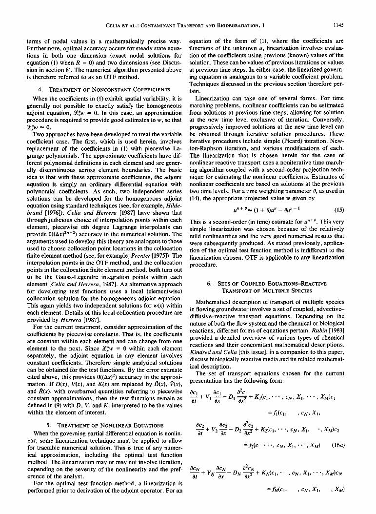
Fig. 3. Comparison of numerical solutions to analytical solu-tions. Solid curves indicate OTF numerical solutions; symbolsindicate analytical solution values.

transport systems. A variety of problems related specifically tobiodegradation are solved in the companion paper [Kindredand Celia, this issue] using the techniques developed herein.Additional test problems for the specific case of advectiondominated, nonreactive transport are reported by Celia et al.[1989a]. Bouloutas and Celia [1988] provide an in-depth nu-merical analysis of a related OTF algorithm for nonreactivetransport of a single species.

In (16), Cl' CZ' ..., CN are measures of aqueous concentrationsof N dissolved species, each of which is hydrodynamicallytransported and has the ability to react with other constituents.The variables Xl, Xz, ..., XM are concentration measures ofreactive species that are stationary. This set of equations istaken to generally correspond to various models of biodegra-dation discussed by Kindred and Celia [this issue]. The presentobjective is to describe the overall numerical algorithm pro-posed to solve the set (16). Kindred and Celia [this issue]provide derivation and physical motivation for the equationforms as well as additional computational details.

The solution procedure adopted herein utilizes the optimaltest function concepts developed in the earlier sections of thispaper. To proceed from one time step to the next, a simple,noniterative linearization is employed. Equation (15) is used toprovide required estimates of the solution for evaluation of thenonlinear reaction coefficients and forcing functions. The pro-jection is applied to each Ci' i= 1,2, ..., N, as well as each Xi,i= 1, 2, ..., M. Let the projected values be denoted with anasterisk. The linearized version of (16) is thus written

7.1. Comparison to Analytical Solutions

Equation (1), with constant coefficients, is solved forseveral different combinations of the coefficients. Threecases are considered: (1) R = I, K = 0; (2) R = 1, K = 0.01;and (3) R = 2, K = 0.01. Each case uses V = 1.0, D = 0.2,f(x,t) = 0.0, and 6x = 2.0, implying a grid Peclet number of10. Initial conditions are fixed as uo(x) = 0, and boundaryconditions are go = 10, gL = o. Figure 3 shows numericalresults for each case, as well as the respective analyticalsolutions. Agreement is excellent in each case. Numericalmass balance errors are less than 1% for the first twosolutions and approximately 1.5% for the third solution.

, c~,xf,

xXt)Ci

= Ji(cf, cN,Xf,

(17a)

XXI)

ax/at + Gj(cf, CN,Xj,

XM)Xi

=Fj(cf,"',CN,Xf,"',XXI) (17b)

These equations are used to moye from the level n to n + 1.Given known values c;*, XJ', each Kj, Gj,fj, and Fj are knownfunctions of space. These spatially variable coefficients arenext approximated by piecewise constants, with each coef-ficient taken as constant within any element. Given thesepiecewise constant values, the adjoint operator is obtainedfor each element. Homogeneous solutions of the adjointequation are subsequently obtained and used as test functionin the optimal test function algorithm. Each transport equa-tion has its own set of test functions, and each equation issolved separately.

The equations for X,{X, t) have no spatial derivatives, imply-ing no coupling in space. As such, these equations are solvedfor each node in space, with no coupling between nodes.Linearization is again based on the projection technique of(15).Use of constant values of Gj and Fj over a time step, based onthe values c;, X;, allows (17b) to be solved analytically.

7.2.

Two-Species Transport

A second example is presented that involves transport oftwo species, coupled through the reaction terms. One sta-tionary component is included, but it is assumed to betemporally static. One physical analogy for this system istransport of two substrates in the presence of a stationarybiological population. Dissolved species might be an organiccontaminant and dissolved oxygen, leading to an aerobicbiodegradation transport problem. Simulations that includetemporal dynamics of the stationary species are included inthe work by Kindred and Celia [this issue].

Governing equations for this system take the form

iJc)/iJt + V iJc)/iJx -D iJZclliJxZ + K)(c), XJc) = h(cz, Xu

iJc7/iJt +ViJc7/iJx -D iJzc7/iJxz + Kz(cz, XJcz =!z(c\, XJ7. EXAMPLE CALCULATIONS

Several example calculations are presented to demonstratethe viability of OTF methods for advective-diffusive-reactive

CELIA ET AL.: CONTAMINANT TRANSPORT AND BIODEGRADATION, I

1147

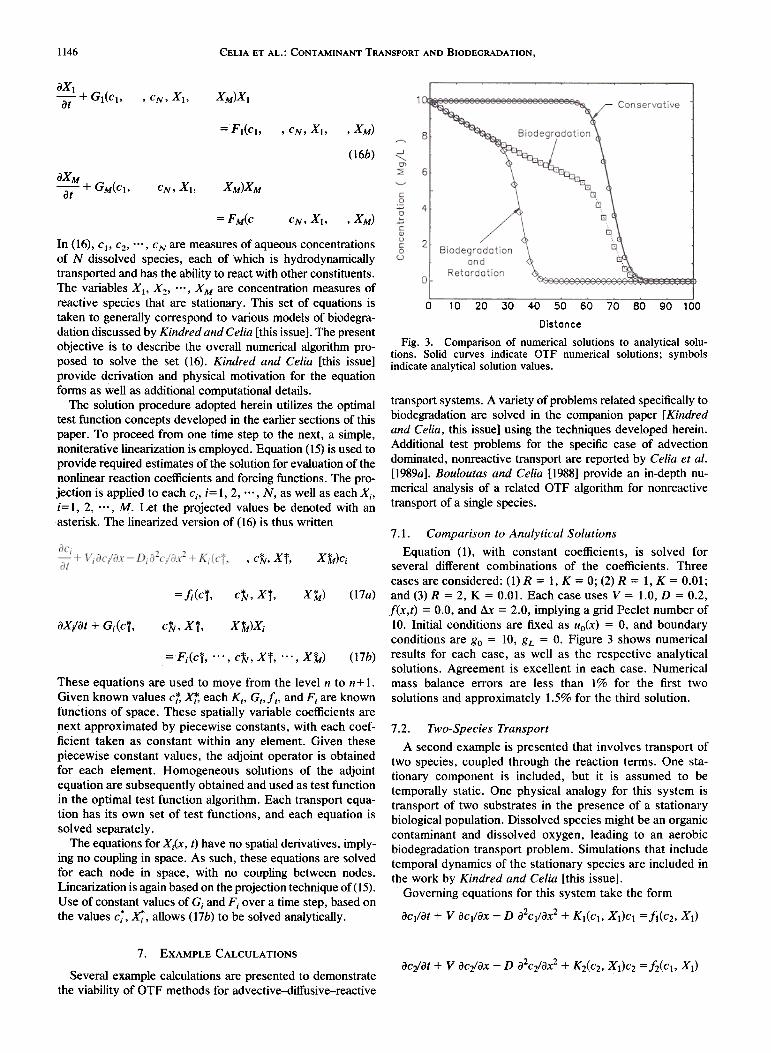
Fig. 4.DISTANCE (m)

Numerical solution of (18) and (19) using OTF. Solutions are plotted at time t = 68 days.

species 2. This error is not a consequence of the timestepping algorithm, because the solution was insensitive totime step reductions. Reduction of the space step Ax from 2m to I m reduced the mass balance errors to less than 3% forspecies I and less than 1 % for species 2. The actual solutionsfor Ax = 2 and Ax = 1 are virtually indistinguishable at t =68 days, with only a slight change evident at the interactingconcentration fronts (the fronts are displaced by approxi-mately 1 m). This appears to be a consequence of thepiecewise constant approximation of the spatially variable(nonlinear) reaction coefficient, which is a relatively poorapproximation in the vicinity of the sharp concentrationfronts. Implementation of the high-order spatial proceduresof Celia and Herrera [1987] or reduction of the space step (asindicated above) will alleviate the mass balance discrepancy.While the mass balance approaches unity as Ax decreases,the numerical solutions for concentrations remain virtuallyindistinguishable from those presented in Figure 4.

8.

DISCUSSION AND CONCLUSIONS

This paper presents a new numerical method for solutionof reactive transport problems. The technique derives fromjudicious

mathematical manipulation of the weak form of thegoverning equations. Special choice of the test functions,based on solution of the homogeneous adjoint equation,leads to an optimal approximation technique. The methodhas the desirable property of automatic adjustment of theapproximation to accommodate varying degrees of diffusion,advection, and reaction domination.

For one-dimensional, steady state problems (ordinarydifferential equations with constant coefficients), the methodproduces exact nodal values for the unknown function and,if desired, its first derivative. Procedures of arbitrarily highorder, on fixed grids, have been developed for the case ofvariable coefficients [Celia and Herrera, 1987; Herrera,1987]. In addition, tensor product test functions applied tothe two-dimensional Laplace equation lead again to anoptimal approximation. This latter case can be shown toproduce a sixth"order approximation using only nine nodepoints [Celia et al., 1989b]. Collatz [1960] has shown thatthis is the highest possible order of approximation for a ninepoint approximation to the Laplace equation. The OTFapproach therefore appears to be a very promising numericalmethod.

Specific functional forms for the nonlinear coefficients arechosen, based on the analogy to biodegradation, as follows:

K1(CI, XJ = (V~xl/(Kl + cJ)81 (19a)

Kz(cz, XJ = (V~XI/(K~ + cz))az (19b)

II (cz, XJ = -KIZ(V;"xI/(K~+ cz))azcz = -KIZKzcz (19c)

h(cl,XJ= -KZI(V:nXI/(Kl + cJ)8lcl = -KZIK1cl (19d)

where physical interpretations are that V:" is the maximumuptake rate for species i, K~, the half-saturation constant forspecies i, Kij is the yield ratio coefficient for species i whenspeciesj is limiting, and 8j is equal to 1 if species i is limitingthe reactions and zero otherwise. Species 1 and 2 areassumed to react in a fixed ratio; this is reflected in thecoefficients Kij. Equations (18) allow either of the species tobe limiting. There is no bacterial growth in this equation (GI= 0), so the stationary species has a fixed value X I. Deriva-

tion and discussion of these equations is provided in thecompanion paper [Kindred and Celia, this issue].

Parameter values are assigned as follows: V:" = 1.0days-I, i = 1, 2; K~ = 0.1 mg/L, i = 1,2; KI2 = 2.0, K21 =0.5. Initial conditions are Cj(X, 0) = 3.0, C2(X, 0) = 0.0.Imposed boundary conditions are CI(O, t) = 3.0, C2(0, t) =10., iJCj/iJx (L, t) = iJC2/iJX (L, t) = 0, where L = 100 m. Thestationary species is fixed at XI = 0.2 mgiL. Flow parame-ters are V = 1.0 rn/day and D = 0.2 m2/day. The system

described by these parameters corresponds to a step intro-duction of species C2 at the left boundary. This propagatesinto the domain by advection and diffusion. Its presenceinstigates uptake of both species 1 and 2. Figure 4 showsplots of concentration as a function of distance for time t =

68 days, for both species 1 and 2, calculated using the OTFalgorithm with grid spacing f).x = 2 m and time step ilt = 0.2

days. The reaction occurs until species I, which is limiting tothe left of the invading front, disappears, at which pointreaction ceases. To the right of the front, species 2 islimiting, due to its initial concentration of zero. The gridPeclet number for this example is 10. This small to interme-diate value of Grid Peclet number is easily accommodated bythe OTF method. This example is expanded in the compan-ion paper of Kindred and Celia [this issue] to include bothinhibited and uninhibited bacterial growth.

Mass balance errors for this two-species example wereapproximately 5% for species 1 and approximately 3% for

1148 CELIA ET AL.: CONTAMINANT TRANSPORT AND BIODEGRADATION,

Current efforts are focusing on improved treatment of thetime domain as well as extensions to multiple spatial dimen-sions. As indi~ated above, initial efforts in multiple dimen-sions using tensor product test functions have produced veryencouraging results. We plan to extend these results to thecase of multidimensional reactive transport. We are alsoinvestigating several formulations that apply the OTF con-cept to the full space-time equation. The companion paper tothis one [Kindred and Celia, this issue] uses the OTFsimulator developed herein as a numerical tool to demon-strate behavior of various biologically reactive subsurfacetransport systems.

Acknowledgments. This work was supported in part by theNational Science Foundation under grant 8657419-CES and by theMassachusetts Institute of Technology under Sloan Foundationgrant 26950.

Herrera, I., Unified approach to numerical methods, I, Green'sformula for operators in discontinuous fields, Numer. MethodsPartial Differential Equations, 1(1), 25-44, 1985a.

Herrera, I., Unified approach to numerical methods, II, Finiteelements, boundary elements, and their coupling, Numer. Meth-ods Partial Differential Equations, 1(3), 159-186, 1985b.

Herrer~, I., The algebraic theory approach for ordinary differentialequations: Highly accurate finite differences, Numer. MethodsPartial Differential Equations, 3(3), 199-218, 1987.

Herrera, I., L. Chargoy, and G. Alducin, Unified approach tonumerical methods, III, Finite differences and ordinary differen-tial equations, Numer. Methods Partial Differential Equations,1(4), 241-258, 1985.

Hildebrand, F. B., Advanced Calculus for Applications, 2nd ed.,Prentice-Hall, Englewood Cliffs, N.J., 1976.

Hughes, T. J. R., and A. Brooks, A theoretical framework forPetrov-Gaierkin methods with discontinuous weighting functions:Applications to the streamlin~-upwind procedure, in Finite Ele-ments in Fluids, vol. 4, edited by R. H. Gallagheretal., pp. 47-65,John Wiley and Sons, New York, 1982.

Kindred, J. S., and M. A. Celia, Contaminant transport and biodeg-radation, 2, Conceptual model and test simulations, Water Re-sour. Res., this issue.

Leonard, B. P., A stable and accurate convective modelling proce-dure based on quadratic upstream interpolation, Compo Meth.Appl. Mech. Eng., 19, 55-98, 1979.

Prenter, P. M., Splines and Variational Methods, 323 pp., JohnWiley and Sons, San Diego, Calif., 1975.

Rubin, J., Transport of reacting solutes in porous media: Relationbetween mathematical nature of problem formulation and chem-ical nature of reactions, Water Resour. Res., 19(5), 1231-1252,1983.

Tezduyar, T. E., and D. K. Ganjoo, Petrov-Gaierkin formulationswith weighting functions dependent upon spatial and temporaldiscretization: Application to transient convective-diffusion prob-lems, Compo Method Appl. Mech. Eng., 59, 49-71, 1986.

M. A. Celia, Parsons Laboratory, Room 48-207, Department ofCivil Engineering, Massachusetts Institute of Technology, Cam-bridge, MA 02139.

I. Herrera, Instituto de Geofisica, National Autonomous Univer-sity of Mexico, Apdo. Postal 22-582, 14000 Mexico D.F., Mexico.

J. S. Kindred, Golder Associates Inc., 4104 148th Avenue North-east, Redmond, W A 98052.

(Received April 21, 1988;revised January 16, 1989;

accepted January 31, 1989.)

REFERENCESBaptista, A. M., Solution of advection-dominated transport by

Eulerian-Lagrangian methods using the backward methods ofcharacteristics, Ph.D. thesis, Dep. of Civ. Eng., Mass. Inst. ofTechnol., Cambridge, Mass., 1987.

Bouloutas, E. T., and M. A. Celia, An analysis of a class ofPetrov-Galerkin and Optimal Test Functions methods, in Proc.Seventh Int. Coni Computational Methods in Water Resources,edited by M. A. Celia et al., pp. 15-20, Elsevier Science, NewYork, 1988.

Carey, G. F., and J. T. Oden, Finite Elements: A Second Course,volume 2, The Texas Finite Element Series, Prentice-Hall, Engle-wood Cliffs, N.J., 1983.

Celia, M. A., and I. Herrera, Solution of general ordinary differen-tial equations by a unified theory approach, Num. MethodsPartial Differential Equations, 3(2), 117-129, 1987.

Celia, M. A., I. Herrera, E. T. Bouloutas, and J. S. Kindred, A newnumerical approach for the advective-diffusive transport equa-tion, Num. Methods Partial Differential Equations, in press,1989a.

Celia.. M. A., I. Herrera, and E. T. Bouloutas, Adjoint Petrov-Galerkin methods for multi-dimensional flow problems, in Proc.Seventh Int. Coni on Finite Element Methods in Flow Problems,pp. 953-958, UAH Press, Huntsville, Ala., 1989b.

Collatz, L., Numerical Treatment of Differential Equations, 3rd ed.,Springer, New York, 1960.

Herrera, I., Boundary Methods: An Algebraic Theory, Pitman,London, 1984.

,