213
Complex Dynamics and Renormalization by Curtis T. McMullen

Complex Dynamics andRenormalization
by
Curtis T. McMullen

Contents
1 Introduction 11.1 Complex dynamics . . . . . . . . . . . . . . . . . . . . 11.2 Central conjectures . . . . . . . . . . . . . . . . . . . . 31.3 Summary of contents . . . . . . . . . . . . . . . . . . . 6
2 Background in conformal geometry 92.1 The modulus of an annulus . . . . . . . . . . . . . . . 102.2 The hyperbolic metric . . . . . . . . . . . . . . . . . . 112.3 Metric aspects of annuli . . . . . . . . . . . . . . . . . 132.4 Univalent maps . . . . . . . . . . . . . . . . . . . . . . 152.5 Normal families . . . . . . . . . . . . . . . . . . . . . . 172.6 Quasiconformal maps . . . . . . . . . . . . . . . . . . 182.7 Measurable sets . . . . . . . . . . . . . . . . . . . . . . 192.8 Absolute area zero . . . . . . . . . . . . . . . . . . . . 202.9 The collar theorem . . . . . . . . . . . . . . . . . . . . 222.10 The complex shortest interval argument . . . . . . . . 272.11 Controlling holomorphic contraction . . . . . . . . . . 30
3 Dynamics of rational maps 353.1 The Julia and Fatou sets . . . . . . . . . . . . . . . . . 363.2 Expansion . . . . . . . . . . . . . . . . . . . . . . . . . 383.3 Ergodicity . . . . . . . . . . . . . . . . . . . . . . . . . 423.4 Hyperbolicity . . . . . . . . . . . . . . . . . . . . . . . 443.5 Invariant line fields and complex tori . . . . . . . . . . 47
4 Holomorphic motions and the Mandelbrot set 534.1 Stability of rational maps . . . . . . . . . . . . . . . . 534.2 The Mandelbrot set . . . . . . . . . . . . . . . . . . . 59
i

5 Compactness in holomorphic dynamics 65
5.1 Convergence of Riemann mappings . . . . . . . . . . . 66
5.2 Proper maps . . . . . . . . . . . . . . . . . . . . . . . 67
5.3 Polynomial-like maps . . . . . . . . . . . . . . . . . . . 71
5.4 Intersecting polynomial-like maps . . . . . . . . . . . . 74
5.5 Polynomial-like maps inside proper maps . . . . . . . 75
5.6 Univalent line fields . . . . . . . . . . . . . . . . . . . 78
6 Polynomials and external rays 83
6.1 Accessibility . . . . . . . . . . . . . . . . . . . . . . . . 83
6.2 Polynomials . . . . . . . . . . . . . . . . . . . . . . . . 87
6.3 Eventual surjectivity . . . . . . . . . . . . . . . . . . . 89
6.4 Laminations . . . . . . . . . . . . . . . . . . . . . . . . 91
7 Renormalization 97
7.1 Quadratic polynomials . . . . . . . . . . . . . . . . . . 97
7.2 Small Julia sets meeting at periodic points . . . . . . . 102
7.3 Simple renormalization . . . . . . . . . . . . . . . . . . 109
7.4 Examples . . . . . . . . . . . . . . . . . . . . . . . . . 113
8 Puzzles and infinite renormalization 117
8.1 Infinite renormalization . . . . . . . . . . . . . . . . . 117
8.2 The Yoccoz jigsaw puzzle . . . . . . . . . . . . . . . . 119
8.3 Infinite simple renormalization . . . . . . . . . . . . . 122
8.4 Measure and local connectivity . . . . . . . . . . . . . 123
8.5 Laminations and tableaux . . . . . . . . . . . . . . . . 125
9 Robustness 129
9.1 Simple loops around the postcritical set . . . . . . . . 129
9.2 Area of the postcritical set . . . . . . . . . . . . . . . . 132
10 Limits of renormalization 135
10.1 Unbranched renormalization . . . . . . . . . . . . . . . 137
10.2 Polynomial-like limits of renormalization . . . . . . . . 140
10.3 Proper limits of renormalization . . . . . . . . . . . . . 145
10.4 Extracting a univalent line field . . . . . . . . . . . . . 150
ii

11 Real quadratic polynomials 16111.1 Intervals and gaps . . . . . . . . . . . . . . . . . . . . 16111.2 Real robustness . . . . . . . . . . . . . . . . . . . . . . 16511.3 Corollaries and generalizations . . . . . . . . . . . . . 168
A Orbifolds 171A.1 Smooth and complex orbifolds . . . . . . . . . . . . . 171A.2 Coverings and uniformization . . . . . . . . . . . . . . 173A.3 The orbifold of a rational map . . . . . . . . . . . . . 177
B A closing lemma for rational maps 181B.1 Quotients of branched coverings . . . . . . . . . . . . . 181B.2 Critically finite rational maps . . . . . . . . . . . . . . 184B.3 Siegel disks, Herman rings and curve systems . . . . . 186B.4 Rational quotients . . . . . . . . . . . . . . . . . . . . 192B.5 Quotients and renormalization . . . . . . . . . . . . . 194
Bibliography 201
Index 207
iii

iv

Chapter 1
Introduction
1.1 Complex dynamics
This work presents a study of renormalization of quadratic polyno-mials and a rapid introduction to techniques in complex dynamics.
Around 1920 Fatou and Julia initiated the theory of iterated ra-tional maps
f : C → C
on the Riemann sphere. More recently methods of geometric func-tion theory, quasiconformal mappings and hyperbolic geometry havecontributed to the depth and scope of research in the field. The in-tricate structure of the family of quadratic polynomials was revealedby work of Douady and Hubbard [DH1], [Dou1]; analogies betweenrational maps and Kleinian groups surfaced with Sullivan’s proof ofthe no wandering domains theorem [Sul3] and continue to informboth subjects [Mc2].
It can be a subtle problem to understand a high iterate of arational map f of degree d > 1. There is tension between expandingfeatures of f — such as the fact that its degree tends to infinity underiteration — and contracting features, such as the presence of criticalpoints. The best understood maps are those for which the criticalpoints tend to attracting cycles. For such a map, the tension isresolved by the concentration of expansion in the Julia set or chaoticlocus of the map, and the presence of contraction on the rest of thesphere.
1

2 Chapter 1. Introduction
The central goal of this work is to understand a high iterate ofa quadratic polynomial. The special case we consider is that of aninfinitely renormalizable polynomial f(z) = z2 + c.
For such a polynomial, the expanding and contracting propertieslie in a delicate balance; for example, the critical point z = 0 belongsto the Julia set and its forward orbit is recurrent. Moreover highiterates of f can be renormalized or rescaled to yield new dynamicalsystems of the same general shape as the original map f .
This repetition of form at infinitely many scales provides the ba-sic framework for our study. Under additional geometric hypotheses,we will show that the renormalized dynamical systems range in acompact family. Compactness is established by combining univer-sal estimates for the hyperbolic geometry of surfaces with distortiontheorems for holomorphic maps.
With this information in hand, we establish quasiconformal rigid-ity of the original polynomial f . Rigidity of f supports conjecturesabout the behavior of a generic complex dynamical system, as de-scribed in the next section.
The course of the main argument entails many facets of com-plex dynamics. Thus the sequel includes a brief exposition of topicsincluding:
• The Poincare metric, the modulus of an annulus, and distortiontheorems for univalent maps (§2);
• The collar theorem and related aspects of hyperbolic surfaces(§2.9 and §2.10);
• Dynamics of rational maps and hyperbolicity (§3.1 and §3.4);
• Ergodic theory of rational maps, and the role of the postcriticalset as a measure-theoretic attractor (§3);
• Invariant line fields, holomorphic motions and stability in fam-ilies of rational maps (§3 and §4);
• The Mandelbrot set (§4);
• Polynomial-like maps and proper maps (§5);
• Riemann mappings and external rays (§5 and §6);

1.2. Central conjectures 3
• Renormalization (§7);
• The Yoccoz puzzle (§8);
• Real methods and Sullivan’s a priori bounds (§11);
• Orbifolds (Appendix A); and
• Thurston’s characterization of critically finite rational maps(Appendix B).
1.2 Central conjectures
We now summarize the main problems which motivate our work.Let f : C → C be a rational map of the Riemann sphere to itself
of degree d > 1. The map f is hyperbolic if its critical points tend toattracting periodic cycles under iteration. Within all rational maps,the hyperbolic ones are among the best behaved; for example, whenf is hyperbolic there is a finite set A ⊂ C which attracts all pointsin an open, full-measure subset of the sphere (see §3.4).
One of the central problems in conformal dynamics is the follow-ing:
Conjecture 1.1 (Density of hyperbolicity) The set of hyperbolicrational maps is open and dense in the space Ratd of all rational mapsof degree d.
Openness of hyperbolic maps is known, but density is not. Insome form this conjecture goes back to Fatou (see §4.1).
Much study has been devoted to special families of rational maps,particularly quadratic polynomials. Every quadratic polynomial f isconjugate to one of the form fc(z) = z2 + c for a unique c ∈ C.Even this simple family of rational maps exhibits a full spectrum ofdynamical behavior, reflecting many of the difficulties of the generalcase. Still unresolved is:
Conjecture 1.2 The set of c for which z2 + c is hyperbolic formsan open dense subset of the complex plane.

4 Chapter 1. Introduction
The Mandelbrot set M is the set of c such that under iteration,fnc (0) does not tend to infinity; here z = 0 is the unique critical pointof fc in C. A component U of the interior of M is hyperbolic if fcis hyperbolic for some c in U . It is known that the maps fc enjoy atype of structural stability as c varies in any component of C− ∂M ;in particular, if U is hyperbolic, fc is hyperbolic for every c in U (see§4). It is clear that fc is hyperbolic when c is not in M , becausethe critical point tends to the superattracting fixed point at infinity.Thus an equivalent formulation of Conjecture 1.2 is:
Conjecture 1.3 Every component of the interior of the Mandelbrotset is hyperbolic.
An approach to these conjectures is developed in [MSS] and[McS], using quasiconformal mappings. This approach has the ad-vantage of shifting the focus from a family of maps to the dynamicsof a single map, and leads to the following:
Conjecture 1.4 (No invariant line fields) A rational map f car-ries no invariant line field on its Julia set, except when f is doublecovered by an integral torus endomorphism.
Conjecture 1.4 implies all the preceding conjectures [McS]. Thisconjecture is explained in more detail in §3.5; see also [Mc3].
The rational maps which are covered by integral torus endomor-phisms form a small set of exceptional cases. For quadratic polyno-mials, Conjecture 1.4 specializes to:
Conjecture 1.5 A quadratic polynomial carries no invariant linefield on its Julia set.
The Julia set J of a polynomial f is the boundary of the set ofpoints which tend to infinity under iteration. A line field on J is theassignment of a real line through the origin in the tangent space toz for each z in a positive measure subset E of J , so that the slope isa measurable function of z. A line field is invariant if f−1(E) = E,and if f ′ transforms the line at z to the line at f(z).
Conjecture 1.5 is equivalent to Conjectures 1.2 and 1.3 (see §4).Recent progress towards these conjectures includes:

1.2. Central conjectures 5
Theorem 1.6 (Yoccoz) A quadratic polynomial which carries aninvariant line field on its Julia set is infinitely renormalizable.
See §8. Here a quadratic polynomial is infinitely renormalizable ifthere are infinitely many n > 1 such that fn restricts to a quadratic-like map with connected Julia set; see §7. For instance, the much-studied Feigenbaum example is an infinitely renormalizable polyno-mial (see §7.4).
This work addresses the infinitely renormalizable case. Our mainresult is:
Theorem 1.7 (Robust rigidity) A robust infinitely renormalizablequadratic polynomial f carries no invariant line field on its Julia set.
See §10. Roughly speaking, a quadratic polynomial is robust if itadmits infinitely many renormalizations with definite space aroundthe small postcritical sets (see §9).
To establish this result, we will show that suitable renormaliza-tions of a robust quadratic polynomial range through a compact setof proper mappings. One may compare our proof of the absence ofinvariant line fields to a fundamental result of Sullivan, which statesthat the limit set of a finitely generated Kleinian group carries no in-variant line field [Sul1]. The compactness of renormalizations plays arole something like the finite-dimensionality of the ambient Lie groupfor a Kleinian group.
It can be shown that every infinitely renormalizable real quadraticpolynomial is robust (§11). When combined with the result of Yoc-coz, we obtain:
Corollary 1.8 The Julia set of a real quadratic polynomial carriesno invariant line field.
From the λ-lemma of [MSS], one obtains:
Corollary 1.9 Every component of the interior of the Mandelbrotset meeting the real axis is hyperbolic.
These corollaries are deduced in §11.

6 Chapter 1. Introduction
1.3 Summary of contents
We begin in §2 with a resume of results from hyperbolic geometry,geometric function theory and measure theory. Then we introducethe theory of iterated rational maps, and study their measurabledynamics in §3.
Here one may see the first instance of a general philosophy:
Expanding dynamics promotes a measurable line field toa holomorphic line field.
This philosophy has precursors in [Sul1] and classical arguments inergodic theory.
In §4 we discuss holomorphic motions and structural stability ingeneral families of rational maps. Then we specialize to the Mandel-brot set, and explain the equivalence of Conjectures 1.2 and 1.5.
In §5, we develop compactness results to apply the expansionphilosophy in the context of renormalization. We also introduce thepolynomial-like maps of Douady and Hubbard, which play a funda-mental role in renormalization.
In §6, we turn to polynomials and describe the use of externalrays in the study of their combinatorics.
With this background in place, the theory of renormalization isdeveloped in §7. New types of renormalization, unrelated to “tun-ing”, were discovered in the course of this development; examples arepresented in §7.4.
§8 describes infinitely renormalizable quadratic polynomials. In-cluded is an exposition of the Yoccoz puzzle, a Markov partition forthe dynamics of a quadratic polynomial. Theorem 1.6 is discussedalong with work of Lyubich and Shishikura.
In §9 we define robust quadratic polynomials, and prove theirpostcritical sets have measure zero. This assertion is essential forapplying the expansion philosophy, because we only obtain expansionin the complement of the postcritical set.
§10 gives the proof of Theorem 1.7(Robust rigidity). The proof isbroken down into two cases. In the first case, the postcritical set fallsinto far-separated blocks at infinitely many levels of renormalization.Using this separation, we extract a polynomial-like map g as a limitof infinitely many renormalizations of a quadratic polynomial f . If

1.3. Summary of contents 7
f carries a measurable invariant line field, the expansion philosophyleads to a well-behaved holomorphic invariant line field for g, whichcan easily be shown not to exist.
In the second case, the blocks of the postcritical set are not well-separated. Then we carry out a parallel argument without attemptingto produce a polynomial-like limit of renormalization. More flexiblelimits of renormalization still suffice to give rigidity of the originalquadratic map. The limit constructed in this case is a proper mapof degree two g : X → Y , between disks X and Y , with the criticalpoint of g inX∩Y . (We do not requireX ⊂ Y .) The dynamics of g issufficiently nonlinear to again rule out the existence of a measurableline field for the original map f .
A useful tool in our study of complex renormalization is the fol-lowing result from hyperbolic geometry. Let X be a surface of finitearea with one cusp and geodesic boundary. Suppose each bound-ary component has length at least L. Then two boundary compo-nents are within distance D(L) of each other (Theorem 2.24). In thecomplex setting, this result will substitute for the “shortest intervalargument” in one dimensional real dynamics.
In §11 we recapitulate and extend arguments of Sullivan to showthat an infinitely renormalizable real quadratic polynomial z2 + c isrobust. This gives Corollaries 1.8 and 1.9 above.
Appendix A provides background on orbifolds, including the uni-formization theorem.
Appendix B further develops the foundations of renormalization,by introducing the notion of a quotient map between two branchedcovers of the sphere. We prove any critically finite quotient of arational map is again rational. This result can be thought of as a‘closing lemma’ for rational maps, although we do not show thatthe critically finite quotient map is near to the original one. Withthis result one may construct an infinite sequence gn of quadraticpolynomials canonically associated to an infinitely renormalizablequadratic polynomial. Conjecturally, gn → f ; this conjecture alsoimplies the density of hyperbolic dynamics in the quadratic family.
Related literature. Basic material on iterated rational maps canbe found in [Fatou1], [Fatou2], [Fatou3], [Julia], [Bro], [Dou1], [McS],[Bl], [Mil2], [EL] [Bea2] and [CG]. A survey of the conjectures in
8 Chapter 1. Introduction
conformal dynamics which motivate this work appears in [Mc3].Renormalization is a broad topic, many aspects of which we do
not touch on here. An exposition of results of Branner, Hubbardand Yoccoz and their relation to complex renormalization appears in[Mil3]. See [Cvi] for a collection of papers on the discovery and de-velopment of renormalization. Fundamental results on compactnessand convergence of renormalization for real quadratic maps appear in[Sul4]; see also [MeSt] for a treatment of Sullivan’s results. Anotherapproach to convergence of renormalization, via rigidity of towers,appears in [Mc2] and [Mc4]. The relation of renormalization to self-similarity in the Mandelbrot set is studied in [Mil1].
The conjectures that we study here are a field of active research;in particular, Lyubich and Swiatek have independently made deepcontributions towards the density of expanding dynamics in the qua-dratic family [Lyu3], [Sw].
A preliminary version of this manuscript was written in summerof 1992. This research was partially supported by the NSF, IHESand the Sloan Foundation.

Chapter 2
Background in conformal
geometry
This chapter begins with standard results in geometric function the-ory, quasiconformal mappings, hyperbolic geometry and measuretheory that will be used in the sequel. These results describe theapproximate geometry of annuli, univalent maps, measurable setsand hyperbolic surfaces. The reader may wish to concentrate on thestatements rather than the proofs, which are sometimes technical.
We also include geometric theorems needed in the sequel that canbe stated without reference to dynamics: a measure zero criterion(§2.8), the collar theorem (§2.9), a complex version of the shortestinterval argument (§2.10) and bounds on holomorphic contraction(§2.11).
Notation. The Riemann sphere and the punctured plane will bedenoted by:
C = C ∪ ∞ and
C∗ = C− 0;
the upper halfplane, unit disk and punctured disk by:
H = z : Im(z) > 0,∆ = z : |z| < 1 and
∆∗ = ∆− 0;
9

10 Chapter 2. Background in conformal geometry
and a family of annuli centered at zero by
A(R) = z : 1 < |z| < R.
The disk of radius r will be denoted by
∆(r) = z : |z| < r,
and the unit circle by
S1 = z : |z| = 1.
A map of pairs f : (A,A′) → (B,B′) means a map f : A → Bsuch that f(A′) ⊂ B′. The restriction of a mapping f to a subset Uwith f(U) ⊂ V will be denoted simply by f : U → V .
O(x) denotes a quantity whose absolute value is bounded by Cxfor some unspecified universal constant C; q ≍ xmeans cx < q < Cx,again for unspecified c, C > 0.
Bounds of the form A < C(B) mean A is bounded by a quantitywhich depends only on B. Different occurrences of C(B) are meantto be independent.
2.1 The modulus of an annulus
Any Riemann surface A with π1(A) ∼= Z is isomorphic to C∗, ∆∗
or the standard annulus A(R) for some R ∈ (1,∞). In case A isisomorphic to A(R), the modulus of A is defined by
mod(A) =logR
2π.
ThusA is conformally isomorphic to a right cylinder of circumferenceone and height mod(A). By convention mod(A) = ∞ in the othertwo cases.
An annulus B ⊂ C is round if it is bounded by concentric Eu-clidean circles (so B has the form z : r < |z − c| < s).
Theorem 2.1 (Round annulus) Any annulus A ⊂ C of sufficientlylarge modulus contains an essential round annulus B with mod(A) =mod(B) +O(1).

2.2. The hyperbolic metric 11
Here essential means π1(B) injects into π1(A), i.e. B separatesthe boundary components of A.
Proof. We may assume C − A consists of two components C andD, where 0 ∈ C and ∞ ∈ D. Let z1 ∈ C maximize |z| over C, andlet z2 ∈ D minimize |z| over D. By Teichmuller’s module theorem[LV, §II.1.3],
mod(A) ≤ 1
πµ
(√|z1|
|z1|+ |z2|
)
where µ(r) is a positive decreasing function of r.1 Thus |z1| < |z2| ifmod(A) is sufficiently large, in which case A contains a round annulusB = z : |z1| < |z| < |z2|. Moreover, once |z1| < |z2| we have
mod(A) ≤ 1
πµ
(√|z1|2|z2|
)
≤ mod(B) +5 log 2
2π
by the inequality µ(r) < log(4/r) [LV, eq. (2.10) in §II.2.3].
An alternative proof can be based on the following fact: anysequence of univalent maps fn : z : 1/Rn < |z| < Rn → C∗, withfn(1) = 1 and with the image of f separating 0 from ∞, convergesto the identity as Rn → ∞.
2.2 The hyperbolic metric
A Riemann surface is hyperbolic if its universal cover is isomorphicto the upper halfplane H. The hyperbolic metric or Poincare metricon such a Riemann surface is the unique complete conformal metricof constant curvature −1.
By the Schwarz lemma [Ah2, §1-2] one knows:
Theorem 2.2 A holomorphic map f : X → Y between hyperbolicRiemann surfaces does not increase the Poincare metric, and f is alocal isometry if and only if f is a covering map.
1In [LV] the modulus of A(R) is defined to be log(R) rather than log(R)/2π.

12 Chapter 2. Background in conformal geometry
The Poincare metric is defined on any region U ⊂ C provided|C − U | > 2. If U is not connected, we define its Poincare metriccomponent by component.
The hyperbolic metric on the upper halfplane H is given by:
ρ =|dz|Im(z)
;
on the unit disk ∆, by:
ρ =2|dz|
1− |z|2 ;
on the punctured disk ∆∗, by:
ρ =|dz|
|z| log(1/|z|) ;
and on the annulus A(R) by:
ρ =π/ logR
sin(π log |z|/ logR)
|dz||z| .
The last two formulas can be verified using the covering maps z +→exp(iz) from H to ∆∗ and z +→ zlogR/πi from H to A(R).
The core curve γ of an annulus X of finite modulus is its uniqueclosed geodesic. The hyperbolic length of γ is related to the modulusby
length(γ) =π
mod(X),
as can be checked by considering the circle |z| =√R that forms the
core curve of A(R).It is useful to keep in mind an approximate picture for the Poincare
metric on an arbitrary region U in the plane. Such a picture is pro-vided by a theorem of Beardon and Pommerenke [BP, Theorem 1],which we formulate as follows.
Let d(z, ∂U) be the Euclidean distance from z to the boundaryof U . Let mod(z, U) denote the maximum modulus of an essentialround annulus in U whose core curve passes through z. If no suchannulus exists, set mod(z, U) = 0.

2.3. Metric aspects of annuli 13
Theorem 2.3 (Poincare metric on a plane region) For any hy-perbolic region U in the plane, the Poincare metric ρ is comparableto
ρ′ =|dz|
d(z, ∂U)(1 + mod(z, U)).
That is, 1/C < (ρ/ρ′) < C for some universal constant C > 0.
This theorem can also be derived from the thick-thin decompo-sition for hyperbolic manifolds and Theorem 2.1 above.
2.3 Metric aspects of annuli
Let V be a Riemann surface which is topologically a disk, and letE ⊂ V have compact closure. It is convenient to have a measurementof the amount of space around E in V . For this purpose we define
mod(E,V ) = sup mod(A) : A ⊂ V is an annulus enclosing E.
(This means E should lie in the compact component of V −A.) Notethat mod(E,V ) = ∞ if V is isomorphic to C or if E is a single point.
Now suppose V is hyperbolic, and let diam(E) denote diameterof E in the hyperbolic metric on V .
Theorem 2.4 The hyperbolic diameter and modulus of E are in-versely related:
diam(E) → 0 ⇐⇒ mod(E,V ) → ∞
anddiam(E) → ∞ ⇐⇒ mod(E,V ) → 0.
More precisely,
diam(E) ≍ exp(−2πmod(E,V ))
when either side is small, while
C1
diam(E)≥ mod(E,V ) ≥ C2 exp(− diam(E))
when the diameter is large.

14 Chapter 2. Background in conformal geometry
Proof. The first estimate follows from existence of a round annulusas guaranteed by Theorem 2.1. The second follows using estimatesfor the Grotzsch modulus [LV, §II.2].
The relation of modulus to hyperbolic diameter is necessarilyimprecise when the diameter is large. For example, for r < 1 thesets E1 = [−r, r] and E2 = ∆(r) have the same hyperbolic diam-eter d in the unit disk, but for r near 1, mod(E1,∆) ≍ 1/d whilemod(E2,∆) ≍ e−d.
The next result controls the Euclidean geometry of an annulus ofdefinite modulus.
A D γ
Figure 2.1. Core geodesic of an annulus.
Theorem 2.5 Let A ⊂ C be an annulus with core curve γ and withmodulus mod(A) > m > 0. Let D the bounded component of C−A.Then in the Euclidean metric,
d(D, γ) > C(m) diam(γ)
where C(m) > 0.
See Figure 2.1.
Proof. Since A contains an annulus of modulus m with the samecore curve, it suffices to prove the theorem when mod(A) = m.

2.4. Univalent maps 15
Let x be a point in D. We may normalize coordinates on C sothat x = 0 and diam(γ) = 1. Let R = exp(2πm). Then A doesnot contain the circle |z| = R, because otherwise mod(A) > m.By further normalizing with a rotation we can assume A ⊂ C −0, R,∞. The hyperbolic length of γ on A is π/m (see §2.2), soby the Schwarz lemma its length is less than π/m in the Poincaremetric on C − 0, R,∞. Since the Euclidean diameter of γ is oneand the hyperbolic metric on C − 0, R,∞ is complete, we haved(γ, 0) > C(m) > 0. Equivalently, d(x, γ) > C(m) diam(γ). Since xwas an arbitrary point in D, the theorem follows.
2.4 Univalent maps
A univalent map f is an injective holomorphic map. The Koebedistortion theorems make precise the fact that a univalent map hasbounded geometry; we summarize this principle as follows:
Theorem 2.6 (Koebe distortion) The space of univalent maps
f : ∆ → C
is compact up to post-composition with automorphisms of C.
This means any sequence of univalent maps contains a subse-quence fn : ∆ → C such that Mn fn converges to a univalent mapf , uniformly on compact subsets of ∆, for some sequence of Mobiustransformations Mn : C → C.
An equivalent and more classical formulation is the following (cf.[Ah2]):
Theorem 2.7 The space S of univalent functions
f : ∆ → C,
normalized by f(0) = 0 and f ′(0) = 1, is compact in the topology ofuniform convergence on compact sets. In particular, for r < 1 andx, y in ∆(r) we have
1
C(r)≤ |f(x)− f(y)|
|x− y| ≤ C(r)
16 Chapter 2. Background in conformal geometry
and1
C(r)≤ |f ′(x)| ≤ C(r)
for all f in S, where C(r) → 1 as r → 0.
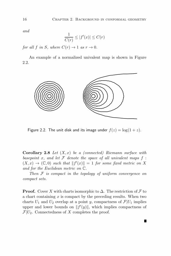
An example of a normalized univalent map is shown in Figure2.2.
Figure 2.2. The unit disk and its image under f(z) = log(1 + z).
Corollary 2.8 Let (X,x) be a (connected) Riemann surface withbasepoint x, and let F denote the space of all univalent maps f :(X,x) → (C, 0) such that ∥f ′(x)∥ = 1 for some fixed metric on Xand for the Euclidean metric on C.
Then F is compact in the topology of uniform convergence oncompact sets.
Proof. CoverX with charts isomorphic to∆. The restriction of F toa chart containing x is compact by the preceding results. When twocharts U1 and U2 overlap at a point y, compactness of F|U1 impliesupper and lower bounds on ∥f ′(y)∥, which implies compactness ofF|U2. Connectedness of X completes the proof.

2.5. Normal families 17
The Koebe principle also controls univalent maps defined on diskswhich are not round. In this case one obtains bounded geometry afterdiscarding an annulus of definite modulus.
Theorem 2.9 Let D ⊂ U ⊂ C be disks with mod(D,U) > m > 0.Let f : U → C be a univalent map. Then there is a constant C(m)such that for any x, y and z in D,
1
C(m)|f ′(x)| ≤ |f(y)− f(z)|
|y − z| ≤ C(m)|f ′(x)|.
Proof. If U = C then f is an affine map and the theorem is immedi-ate with C(m) = 1. Otherwise, let g : (∆, 0) → (U, x) be a Riemannmapping. Then mod(g−1(D),∆) = mod(D,U) > m > 0, so thereis an r(m) < 1 such that g−1(D) ⊂ ∆(r(m)) by Theorem 2.4. Nowapply the Koebe theorem for univalent maps on the unit disk to gand f g.
2.5 Normal families
Definition. Let X be a complex manifold, and let F be a family ofholomorphic maps f : X → C. Then F is a normal family if everysequence fn in F has a subsequence which converges uniformly oncompact subsets of X. The limit f∞ is again a holomorphic map toC.
Theorem 2.10 (Montel) For any complex manifold, the set of allholomorphic maps into C− 0, 1,∞ is a normal family.
The proof is based on the Schwarz Lemma and the fact that thetriply-punctured sphere is covered by the unit disk.
Montel’s theorem is one of the basic tools used in the classicaltheory of iterated rational maps developed by Fatou and Julia. It iseasy to see that any three distinct points on the Riemann sphere canreplace the triple 0, 1,∞ in the statement of the theorem. Moregenerally, we have:

18 Chapter 2. Background in conformal geometry
Corollary 2.11 Let si : X → C, i = 1, 2, 3 be three holomorphicmaps whose graphs are disjoint. Then the set F of all holomor-phic maps f : X → C whose graphs are disjoint from the graphs ofs1, s2, s3 is a normal family.
Proof. There is a holomorphically varying Mobius transforma-tion A(x) mapping s1(x), s2(x), s3(x) to 0, 1,∞. A sequencefn in F determines a sequence gn(x) = A(x)(fn(x)) mapping Xinto the sphere and omitting the values 0, 1 and ∞. Thus gn hasa convergent subsequence gnk
, so fn has a convergent subsequencefnk
(x) = A(x)−1(gnk(x)).
See [Bea2, §3.3], [Mon].
2.6 Quasiconformal maps
We will have occasional need for the theory of quasiconformal maps;basic references for the facts summarized below are [AB], [Ah1] and[LV].
Definition. A homeomorphism f : X → Y between Riemann sur-faces X and Y is K-quasiconformal, K ≥ 1 if for all annuli A ⊂ X,
1
Kmod(A) ≤ mod(f(A)) ≤ Kmod(A).
This is equivalent to the following analytic definition: f is K-quasiconformal if locally f has distributional derivatives in L2, andif the complex dilatation µ, given locally by
µ(z)dz
dz=
∂zf
∂zf=
∂f/∂z
∂f/∂z
dz
dz,
satisfies |µ| ≤ (K− 1)/(K+1) almost everywhere. Note that µ is anL∞ Beltrami differential, that is a form of type (−1, 1).
A mapping f is 1-quasiconformal if and only if f is conformal inthe usual sense.
The great flexibility of quasiconformal maps comes from the factthat any µ with ∥µ∥∞ < 1 is realized by a quasiconformal map. Thisis the “measurable Riemann mapping theorem”:
2.7. Measurable sets 19
Theorem 2.12 (Ahlfors-Bers) For any L∞ Beltrami differentialµ on the plane with ∥µ∥∞ < 1, there is a unique quasiconformal mapφ : C → C such that φ fixes 0 and 1 and the complex dilatation of φis µ.
Moreover, for any µ with ∥µ∥∞ ≤ 1, we may construct a familyof quasiconformal maps φt : C → C, |t| < 1, satisfying
∂zφt∂zφt
= tµ
and normalized as above. Then φt(z) is a holomorphic function oft ∈ ∆ for each z ∈ C.
Amapping preserving the measurable complex structure specifiedby µ can be viewed as holomorphic after a quasiconformal change ofcoordinates. Here is an application to rational maps that we will usein §4.2:
Theorem 2.13 Let f : C → C be a rational map, and let µ be aBeltrami differential on the sphere such that f∗µ = µ and ∥µ∥∞ <1. Then g = φ f φ−1 is also a rational map, where φ is anyquasiconformal map with complex dilatation µ.
Proof. Using the chain rule one may check that g is 1-conformal,hence holomorphic, away from its branch points. The latter areremovable singularities.
This principle forms the basis for the no wandering domains the-orem and for the Teichmuller theory of rational maps [Sul3], [McS].
2.7 Measurable sets
The small scale geometry of a measurable set is controlled by:
Theorem 2.14 (Lebesgue density) Let E ⊂ C be a measurableset of positive area. Then
limr→0
area(E ∩B(x, r))
areaB(x, r)= 1
for almost every x in E.

20 Chapter 2. Background in conformal geometry
See, e.g. [Stein, §I.1]. Here B(x, r) is a ball about x of radiusr in the spherical metric, and area denotes spherical area. Any twosmooth metrics in the same conformal class result in the same limitabove.
Corollary 2.15 Let f : C → Rn be a measurable function. Thenfor all ϵ > 0 and almost every x in C,
limr→0
area(y ∈ B(x, r) : |f(y)− f(x)| < ϵ)areaB(x, r)
= 1.
When the limit above is equal to one for every ϵ > 0, we say f isalmost continuous at x.
2.8 Absolute area zero
It is sometimes useful to study a compact set F ⊂ C in terms of theRiemann surface X = C − F . In this section we give a criterion forF to be a set of area zero, using the conformal geometry of X.
Definitions. The set F is of absolute area zero if the area of C−f(X)is zero for any injective holomorphic map f : X → C. In terms of theclassification of Riemann surfaces, this is equivalent to the conditionthat X is in OAD [SN, p.3].
Since our area criterion will depend only on the conformal geom-etry of X, it will also show F is of absolute area zero.
A set A is nested inside an annulus B ⊂ C if A lies in the boundedcomponent of C−B.
Theorem 2.16 Suppose E1, E2, . . . is a sequence of disjoint opensets in the plane, such that
1. En is a finite union of disjoint unnested annuli of finite moduli;
2. any component A of En+1 is nested inside some component Bof En; and
3. for any sequence of nested annuli An, where An is a componentof En, we have
∑mod(An) = ∞.

2.8. Absolute area zero 21
Let Fn be the union of the bounded components of C − En, and letF =
⋂Fn. Then F is a totally disconnected set of absolute area zero.
The set F consists of those points which are nested inside in-finitely many components of
⋃En.
Lemma 2.17 Let U ⊂ C be a disk of finite area, let K ⊂ U be aconnected compact set, and let A be the annulus U −K. Then
area(K) ≤ area(U)
1 + 4πmod(A).
Proof. Let Γ be the collection of simple closed curves in A whichrepresent the generator of π1(A). By the method of extremal length,the modulus of A satisfies
mod(A) ≤∫A ρ
2(z)|dz|
infγ∈Γ(∫
γ ρ(z)|dz|)2
for any finite area conformal metric ρ(z)|dz| on A [Ah1, p.13]. Takingρ to be the Euclidean metric, the numerator above becomes area(A),while the isoperimetric inequality gives (
∫γ |dz|)2 ≥ 4π area(K) for
every γ in Γ. Since area(A) = area(U)− area(K), we have
mod(A) ≤ area(U)− area(K)
4π area(K),
and the proof is completed by algebra.
Proof of Theorem 2.16. Form a tree (or forest) whose vertices arethe components of
⋃En and whose edges join A ⊂ En to B ⊂ En+1
if B is nested inside A. If we weight each vertex A by mod(A), thenthe sum of the weights along any branch leading to infinity is infinite.Since the tree has finite degree, it follows that Mn → ∞, where
Mn = infAn
n∑
1
mod(Ai)

22 Chapter 2. Background in conformal geometry
and An denotes the collection of all sequences of nested annuli A1,. . . , An such that Ai is a component of Ei.
Using the area-modulus estimate above, one may prove by induc-tion that
area(Fn) ≤ area(F1) supAn
n∏
1
1
1 + 4πmod(Ai),
which tends to zero because Mn tends to infinity. Thus area(F ) = 0.If f : C − F → C is a univalent map, then we may apply the
same argument to f(Ei) to show the complement of the image of falso has area zero. Therefore F has absolute area zero.
Since any component K of F lies in a descending nest of an-nuli with
∑mod(An) = ∞, K is a point and therefore F is totally
disconnected.
Remark. We first formulated this criterion for application to cubicpolynomials in [BH, §5.4]; compare [Mil3]. Lyubich applies the samecriterion to quadratic polynomials in [Lyu4]. A related result appearsin [SN, §I.1.D].
2.9 The collar theorem
Let S(x) be the function
S(x) = sinh−1(1/ sinh(x/2)).
For a simple geodesic α on a hyperbolic surface, the collar about αis given by
C(α) = x : d(x,α) < S(ℓ(α))
where d(·) denotes the hyperbolic metric.The following result is due to Buser [Bus1].
Theorem 2.18 (Collars for simple geodesics) The collar C(α)about a simple geodesic on a hyperbolic surface is an embedded an-nulus.
If α and β are disjoint simple geodesics, then C(α) and C(β) aredisjoint.

2.9. The collar theorem 23
γ
β
δ
α
A
B
Figure 2.3. Distance between simple geodesics.
Proof. For the first part, pass to the universal cover H of X, let αbe a lift of α, and let g ∈ π1(X) be a hyperbolic isometry generatingthe stabilizer of α. If the collar C(α) is not embedded, then there isa point x ∈ α and an h ∈ π1(X) such that d(x, hx) < 2S(x) and hdoes not lie in the cyclic group generated by g. By a trigonometryargument,
sinh(d(x, gx)/2) sinh(d(x, hx)/2) ≥ 1,
[Bea1, Theorem 8.3.1], which is impossible because
sinh(ℓ(α)/2) sinh(S(ℓ(α))) = 1.
Now let α and β be disjoint simple closed curves; to verify thesecond part we will show d(α,β) ≥ S(ℓ(α)) + S(ℓ(β)).
Let γ be a geodesic segment of minimal length joining α to β. Wemay replace X by the covering space Y corresponding to π1(α∪β∪γ),which is a pair of pants. Two ends of Y correspond to α and β; sinceinclusions are contracting, it suffices to prove the inequality when thethird end is a cusp. Let δ be the simple geodesic starting and endingin the cusp. Then δ cuts γ into two segments of length A and B (seeFigure 2.3). We can construct a quadrilateral with three right angles

24 Chapter 2. Background in conformal geometry
and one ideal vertex, whose side lengths are (ℓ(α/2), A,∞,∞). Forsuch a quadrilateral,
sinh(ℓ(α)/2) sinh(A) = 1
[Bea1, Theorem 7.17.1]. Thus A = S(ℓ(α)). A similar argumentgives B = S(ℓ(β)), and A+B = ℓ(γ) = d(α,β).
Theorem 2.19 The modulus of the collar satisfies
modC(α) = M(ℓ(α)) > 0,
where M(x) decreases continuously from infinity to zero as x in-creases from zero to infinity.
Proof. Since the width of C(α) decreases as the length of α in-creases, the modulus M(x) is a decreasing function. Its limitingbehavior follows from the behavior of S(x).
Definition. A cusp is a finite volume end of a (noncompact) hyper-bolic surface.
A cusp is like a neighborhood of a simple geodesic whose lengthhas shrunk to zero. As the length of a geodesic γ tends to zero,each boundary component of the collar C(γ) tends to a horocycle oflength 2. A limiting version of the Collar Theorem 2.18 yields:
Theorem 2.20 (Collars for cusps) Every cusp κ of a hyperbolicsurface X has a collar neighborhood C(κ) ⊂ X isometric to the quo-tient of the region
z : Im(z) > 1 ⊂ H
by the translation z +→ z + 2.The collars about different cusps are disjoint, and C(κ) is disjoint
from the collar C(γ) about any simple geodesic γ on X.

2.9. The collar theorem 25
Definition. The injectivity radius r(x) at a point in a hyperbolicsurface X is the radius of the largest embedded hyperbolic ball cen-tered at x. Equivalently, 2r(x) is the length of the shortest essentialloop on X passing through x.
Theorem 2.21 (Thick-thin decomposition) Let X be a hyper-bolic surface. There is a universal ϵ0 > 0 such that all simplegeodesics of length less than ϵ0 are disjoint, and every point x withinjectivity radius less than ϵ0/2 belongs to the collar neighborhood ofa unique cusp or short geodesic.
Proof. As the length ℓ(γ) of a geodesic γ tends to zero the distancebetween the boundary components of its collar C(γ) tends to infinity,so all sufficiently short geodesics are disjoint. Through any pointx ∈ X there is a simple essential loop of length 2r(x), isotopic to aunique cusp or geodesic on X. Since the injectivity radius is boundedbelow near the boundary of the collar about a short geodesic or cusp,x itself belongs to the interior of the corresponding collar when r(x)is sufficiently small.
For more details see [Bus2, Ch.4, §4.4], [BGS], and [Yam].
Corollary 2.22 There is a universal C > 0 such that for any twopoints x and y on a hyperbolic surface X, the injectivity radius sat-isfies
| log r(x)− log r(y)| ≤ Cd(x, y).
In other words, the log of the injectivity radius is uniformly Lipschitz.
Proof. It is obvious that r(x) is Lipschitz with constant 1, so log r(x)is Lipschitz if r(x) is not too small. But when r(x) is small, x belongsto a standard collar by the thick-thin decomposition, and there theLipschitz property can be verified directly.

26 Chapter 2. Background in conformal geometry
We conclude this section with an estimate of the distance of asmooth loop from its geodesic representative.
Theorem 2.23 Let X be a hyperbolic surface, and let x be a pointon a loop δ ⊂ X which is homotopic to a geodesic γ. Then:
cosh2(d(x, γ)) ≤ cosh2(ℓ(δ)/2) − 1
cosh2(ℓ(γ)/2) − 1.
In particular, a lower bound on ℓ(γ) and an upper bound on ℓ(δ)gives an upper bound on the distance from x to γ.
gx′x′
θ
y gyA
B
D
C
Figure 2.4. Distance to a geodesic.
Proof. Let X = H/π1(X) present X as a quotient of the hyperbolicplane by a discrete group of isometries. Choose a lift of γ to ageodesic γ′ in H, and a compatible lift of x to a point x′ (using thehomotopy from δ to γ). Then there is a g ∈ π1(X) stabilizing γ′ andtranslating it distance ℓ(γ) , and d(x′, gx′) ≤ ℓ(δ) because x′ and gx′
are connected by a lift of δ.Let y and gy be the points nearest to x′ and gx′ on γ′ ⊂ H. Taking
the perpendicular bisector of the geodesic segment from y to gy, wecan form a quadrilateral with three right angles, three sides of lengthA = ℓ(γ)/2, B = d(x′, gx′)/2 ≤ ℓ(δ)/2, and D = d(x′, γ) = d(x, γ),and angle θ between sides B and D (see Figure 2.4). By hyperbolic

2.10. The complex shortest interval argument 27
trigonometry [Bea1, §7.17], we have the relations
sin θ = coshA/ coshB
sin θ = coshC/ coshD
cos θ = sinhC sinhB;
squaring and solving for cosh2(D) gives the theorem.
2.10 The complex shortest interval argument
Any finite collection of disjoint intervals on the real line contains ashortest member I. In real dynamics one may capitalize on the factthat I is shorter than its neighboring intervals; for example, this factwill be used in §11, and it appears in many other one-dimensionalarguments.
In this section we establish a result about hyperbolic surfacesinspired by this shortest interval argument.
Theorem 2.24 (Complex shortest interval) Let X be a finitelyconnected planar hyperbolic surface with one cusp, whose remainingends are cut off by geodesics γ1, . . . γn, n > 1. Suppose the length ofevery γi is greater than L > 0. Then there are two distinct geodesicssuch that
d(γj , γk) ≤ D(L).
Proof. Let X ′ be the complete surface with geodesic boundary ob-tained as the closure of the finite volume component of X−
⋃γi. By
the Gauss-Bonnet theorem, the hyperbolic area of X ′ is −2πχ(X ′) =2π(n − 1). We will construct disjoint neighborhoods Ei of γi whosearea can be estimated.
LetD be the minimum distance between any two geodesics among⟨γi⟩. By the thick-thin decomposition (Theorem 2.21) there is anϵ0 > 0 such that any loop of length less than ϵ0 on a hyperbolic sur-face lies in a collar neighborhood of a unique simple geodesic or cusp.
28 Chapter 2. Background in conformal geometry
Let ϵ = min(ϵ0, L, S−1(D/2)), where S(x) is the function which ap-pears in the collar lemma (see §2.9). Let Σ be the union of the simplegeodesics of length less than ϵ.
The Ei are constructed as follows.
(a) If there is a component of X ′−Σ containing a uniquecurve γi, set Ei equal to this component.
(b) Otherwise, let Ei = Ci(D/2) where
Ci(r) = x ∈ X ′ : d(x, γi) < r.
In case (a), Ei is a complete hyperbolic surface with geodesicboundary, so area(Ei) ≥ 2π.
In case (b), note that for 0 < r < D/2, the length of ∂0Ci(r) =∂Ci(r) − γi is greater than ϵ. For otherwise every component of∂0Ci(r) is homotopic to a short geodesic or the unique cusp of X ′,and we are in case (a). Since
d area(Ci(r))
dr= length(∂0Ci(r)),
we have area(Ei) ≥ ϵD/2 in case (b).
The regions Ei obtained in this way are disjoint. Indeed, it isclear that two regions of type (a) cannot meet, nor can two regionsof type (b), since d(γi, γj) ≥ D. Finally a region of type (b) cannotmeet one of type (a), because every curve in Σ is distance at leastD/2 from every γi. This follows from the Collar Theorem 2.18 andthe fact S(ϵ) ≥ D/2.
Therefore∑n
1 area(Ei) ≤ area(X ′) = 2π(n− 1). Consequently atleast one Ei is of type (b), with 2π ≥ area(Ei) ≥ Dϵ/2, so D ≤ 4π/ϵ.Since ϵ only depends on L, the theorem follows.

2.10. The complex shortest interval argument 29
Figure 2.5. All boundary components are far apart.
Remarks.
1. The importance of the preceding result is that the bound ond(γi, γj) is independent of n.
2. This result is related to the real shortest interval argument asfollows. Suppose X = C −
⋃n1 Ii, where Ii are disjoint closed
intervals on the real axis. Then the geodesics γj and γk en-closing the shortest interval and one of its neighbors will be abounded distance apart whenever we have a lower bound onℓ(γi).
3. An alternate approach to the result above is to realize X as thecomplement of a finite set of round disks D1, . . . Dn in C (anyfinitely connected planar surface with one cusp can be so real-ized — see [Bie, p.221]). Then γj and γk can be chosen as thegeodesics enclosing Dj and Dk, the disk of smallest diameterand its nearest neighbor.
4. The result fails if X is allowed to have two or more cusps (seeFigure 2.5).

30 Chapter 2. Background in conformal geometry
2.11 Controlling holomorphic contraction
Definitions. Let f : X → Y be a holomorphic map between hyper-bolic Riemann surfaces. Let ∥f ′∥ denote the norm of the derivativewith respect to the hyperbolic metrics on domain and range, anddefine the real log derivative of f by
Df(x) = log ∥f ′(x)∥.
By the Schwarz Lemma, ∥f ′(x)∥ ≤ 1 so Df(x) ≤ 0. The functionDf is an additive cocycle in the sense that
D(f g)(x) = Dg(x) +Df(g(x)).
If f ′(x) = 0 we set Df(x) = −∞.In this section we bound the variation of ∥f ′(x)∥ (or equivalently
Df(x)) as the point x varies. To this end it is useful to introducethe 1-form
Nf(x) = d(Df(x)),
the real nonlinearity of f , which measures the infinitesimal variationof ∥f ′∥. Then for any x1 and x2 in X, we have
|Df(x1)−Df(x2)| ≤∣∣∣∣
∫
γNf(z)|dz|
∣∣∣∣ ≤ d(x1, x2) supγ
∥Nf∥,
where γ is a minimal geodesic joining x1 to x2 and ∥Nf∥ denotesthe norm of the real nonlinearity measured in the hyperbolic metricon X.
Example. Let f : ∆ → ∆ be a holomorphic map with f(0) = 0.Then an easy calculation shows:
Df(0) = log |f ′(0)| and ∥Nf(0)∥ =
∣∣∣∣f ′′(0)
2f ′(0)
∣∣∣∣ .
For our applications the most important case is that of an inclu-sion f : X → Y . We begin by showing ∥f ′(x)∥ is small if x is closeto the boundary of X in Y .

2.11. Controlling holomorphic contraction 31
Theorem 2.25 Let f : X ⊂ Y be an inclusion of one hyperbolicRiemann surface into another, and let s = d(x, Y −X) in the hyper-bolic metric on Y . Then if s < 1/2 we have
∥f ′(x)∥ = O(|s log s|).
In particular ∥f ′(x)∥ → 0 as s → 0.
Proof. By the Schwarz lemma we can reduce to the extremal caseY = ∆, X = ∆∗, x > 0 and s = d(0, x) in the hyperbolic metric on∆. As s → 0 we have x ∼ s/2 and
∥f ′(x)∥ = ρ∆(x)/ρ∆∗(x) =2|x log x|1− x2
∼ |s log s|,
where ρ∆ and ρ∆∗ are the hyperbolic metrics on the disk and punc-tured disk.
Now we turn to the variation of ∥f ′(x)∥.
Theorem 2.26 Let f : X → Y be a holomorphic map between hy-perbolic Riemann surfaces such that f ′ is nowhere vanishing. Then
∥Nf(x)∥ = O(|Df(x)|).
Proof. Passing to the universal covers of domain and range, itsuffices to treat the case where X = Y = ∆, x = 0 and f : ∆ → ∆ isa holomorphic map without critical points such that f(0) = 0. SinceDf(x) = log |f ′(0)| and ∥Nf(x)∥ = |f ′′(0)|/(2|f ′(0)|), we are seekinga bound of the form
|f ′′(0)| ≤ C|f ′(0) log |f ′(0)||.
We treat two cases, depending on whether or not |f ′(0)| is closeto one.
First we write f(z) = zg(z), where g : ∆ → ∆ is also holo-morphic, g(0) = f ′(0) and f ′′(0) = 2g′(0). By the Schwarz lemmaapplied to g, we obtain
|f ′′(0)| = |2g′(0)| ≤ 2(1 − |g(0)|2) = 2(1− |f ′(0)|2).

32 Chapter 2. Background in conformal geometry
For 1/2 ≤ x ≤ 1 we have 1− x2 = O(|x log(x)|), so this bound is ofthe required form when |f ′(0)| ≥ 1/2.
Now we treat the case when |f ′(0)| is small; here we will use thefact that f ′ is nonvanishing.
By the Schwarz lemma applied to f , we have
|f ′(z)| ≤ 1− |f(z)|2
1− |z|2≤ 4
3
for z ∈ ∆(1/2), the disk of radius 1/2 centered at the origin. Sincef ′ is nonvanishing, it restricts to a map f ′ : ∆(1/2) → ∆(4/3)− 0.Thus we obtain a holomorphic map h : ∆ → ∆∗ by setting h(z) =(3/4)f ′(z/2). Since the hyperbolic metric on the punctured disk ∆∗
is given by |dz|/|z log |z||, the Schwarz lemma applied to h yields
|h′(0)| =3
8|f ′′(0)| ≤ 2|h(0) log |h(0)|| =
3
2
∣∣∣∣f′(0) log
3
4|f ′(0)|
∣∣∣∣ .
For 0 < x < 1/2 we have | log(3x/4)| = O(| log x|), so this bound isof the desired form when |f ′(0)| < 1/2. Combining these two caseswe obtain the theorem.
Integrating this bound, we obtain:
Corollary 2.27 (Variation of contraction) For any two pointsx1, x2 ∈ X,
∥f ′(x1)∥1/α ≥ ∥f ′(x2)∥ ≥ ∥f ′(x1)∥α
where α = exp(Cd(x1, x2)) for a universal constant C > 0, and d(·)denotes the hyperbolic metric on X.
Proof. By the preceding theorem, the norm of the one-form
Nf(x)
Df(x)= d log |Df(x)|
is bounded by a universal constant with respect to the hyperbolicmetric on X. Thus
| log |Df(x1)|− log |Df(x2)|| ≤ Cd(x1, x2),
which is equivalent to the Corollary.

2.11. Controlling holomorphic contraction 33
We can summarize these bounds by saying that for any holomor-phic immersion f : X → Y between hyperbolic Riemann surfaces,
log log(
1
∥f ′(x)∥
)
is a Lipschitz function on X with uniform Lipschitz constant. Inparticular, if f is only moderately contracting at x ∈ X, then f isnot very contracting within a bounded distance of x.
A prototypical example is provided by the inclusion f : ∆∗ → ∆;as z tends to zero along a hyperbolic geodesic in∆∗, log log(1/∥f ′(z)∥)grows approximately linearly with respect to distance along the geo-desic, so the bounds above are the right order of magnitude.
Next we will show for an arbitrary inclusion f : X → Y , thebounds above can be improved on the thick part of X. In otherwords, the rapid variation of f ′ for the map ∆∗ → ∆ is accountedfor by the small injectivity radius near the cusp.
Theorem 2.28 Let f : X → Y be an inclusion between hyperbolicRiemann surfaces. Then
∥Nf(x)∥ = O(
1
min(1, r(x))
),
where r(x) is the injectivity radius of X at x. In particular, a lowerbound on r(x) gives an upper bound on ∥Nf(x)∥.
Proof. As before we pass to universal covers of domain and rangeand normalize so x = f(x) = 0; then we obtain a map f : ∆ → ∆such that f is injective on the hyperbolic ball B of radius r(x) aboutthe origin. We have B = ∆(s) where s ≍ r(x) when r < 1. Themap h : ∆ → ∆ given by h(z) = f(sz) is univalent. By Koebecompactness of univalent maps, |h′′(0)/h′(0)| < C for a universalconstant C. Since h′′(0)/h′(0) = sf ′′(0)/f ′(0), we obtain ∥Nf(x)∥ ≤C/s = O(1/r(x)) when r(x) < 1.
When r(x) > 1 the same argument gives ∥Nf(x)∥ = O(1).

34 Chapter 2. Background in conformal geometry
For our applications the qualitative version below is easiest to ap-ply. Note that this Corollary improves Corollary 2.27 when ∥f ′(x1)∥is small.
Corollary 2.29 Let f : X → Y be an inclusion between hyperbolicsurfaces. Then for any x1 and x2 in X,
1
C(r, d)≤ ∥f ′(x1)∥
∥f ′(x2)∥≤ C(r, d)
where C(r, d) > 0 is a continuous function depending only on theinjectivity radius r = r(x1) and the distance d = d(x1, x2) betweenx1 and x2.
Proof. Let γ be a path of length d(x1, x2) joining x1 to x2. ByCorollary 2.22, the injectivity radius r(x) is bounded below along γin terms of d(x1, x2) and r(x1). By the preceding result, we obtain anupper bound on ∥Nf(x)∥ along γ. The integral of this bound controls|Df(x1)−Df(x2)|, and thereby the ratio ∥f ′(x1)∥/∥f ′(x2)∥.

Chapter 3
Dynamics of rational
maps
This chapter reviews well-known features of the topological dynam-ics of rational maps, and develops general principles to study theirmeasurable dynamics as well.
We first recall some basic results in rational dynamics (§3.1). Arational map f of degree greater than one determines a partition ofthe Riemann sphere into a pair of totally invariant sets, the Juliaset J(f) and the Fatou set Ω(f). The behavior of f on the Fatouset is well understood: every component eventually cycles, and thecyclic components are the basins of attracting or parabolic cycles, orrotation domains (Siegel disks or Herman rings).
The dynamics on the Julia set is more mysterious in general. Forexample, we do not know if f is ergodic whenever the Julia set isequal to the whole Riemann sphere. We will see, however, that animportant role is played by the postcritical set P (f), defined as theclosure of the forward orbits of the critical points.
In §3.2, we use the hyperbolic metric on C − P (f) to establishexpanding properties of f outside of the postcritical set. In §3.3 thisexpansion leads to the following dichotomy: a rational map eitheracts ergodically on the sphere, or its postcritical set behaves as ameasure-theoretic attractor. The main idea of §3.3 appears in [Lyu1].
Hyperbolic rational maps are introduced in §3.4, and we use theresults just developed to show their Julia sets have measure zero.
35

36 Chapter 3. Dynamics of rational maps
In §3.5 we turn to an analysis of invariant measurable line fieldssupported on the Julia set. We first present the known examples ofrational maps admitting invariant line fields, namely those which arecovered by integral torus endomorphisms. (Examples of this typeare due to Lattes [Lat].) Then we show for any other example, thepostcritical set must act a measure-theoretic attractor for points inthe support of the line field.
This conclusion will later form the first step in our proof that arobust quadratic polynomial is rigid.
3.1 The Julia and Fatou sets
Let f : C → C be a rational map of degree greater than one.
Definitions. A point z such that fp(z) = z for some p ≥ 1 is aperiodic point for f . The least such p is the period of z. If f i(z) =f j(z) for some i > j > 0 we say z is preperiodic.
A periodic cycle A ⊂ C is a finite set such that f |A is a transitivepermutation. The forward orbit of a periodic point is a periodiccycle.
The multiplier of a point z of period p is the derivative (fp)′(z) ofthe first return map. The multiplier provides a first approximationto the local dynamics of fp. Accordingly, we say z is
repelling if |(fp)′(z)| > 1;indifferent if |(fp)′(z)| = 1;attracting if |(fp)′(z)| < 1; andsuperattracting if (fp)′(z) = 0.
An indifferent point is parabolic if (fp)′(z) is a root of unity.
Remark. By the definition above, attracting includes superattract-ing as a special case. This convention is not uniformly adopted inthe literature on rational maps, but it is convenient for our purposes.
The Fatou set Ω(f) ⊂ C is the largest open set such that theiterates fn|Ω : n ≥ 1 form a normal family.
The Julia set J(f) is the complement of the Fatou set.The Julia and Fatou sets are each totally invariant under f ; that
is, f−1(J(f)) = J(f) and f−1(Ω(f)) = Ω(f); so the partition C =J(f) 4 Ω(f) is preserved by the dynamics.

3.1. The Julia and Fatou sets 37
The Julia set is the locus of expanding and chaotic behavior; forexample:
Theorem 3.1 The Julia set is equal to the closure of the set of re-pelling periodic points. It is also characterized as the minimal closedsubset of the sphere satisfying |J | > 2 and f−1(J) = J .
On the other hand, a normal family is precompact, so one mightimagine that the forward orbit of a point in the Fatou set behavespredictably. Note that f maps each component of the Fatou set toanother component. The possible behaviors are summarized in thefollowing fundamental result.
Theorem 3.2 (Classification of Fatou components) Every com-ponent U of the Fatou set is preperiodic; that is, f i(U) = f j(U) forsome i > j > 0. The number of periodic components is finite.
A periodic component U , with fp(U) = U , is of exactly one thefollowing types:
1. An attracting basin: there is an attracting periodic point w inU , and fnp(z) → w for all z in U as n → ∞.
2. A parabolic basin: there is a parabolic periodic point w ∈ ∂Uand fnp(z) → w for all z in U .
3. A Siegel disk: the component U is a disk on which fp acts byan irrational rotation.
4. A Herman ring: the component U is an annulus, and again fp
acts as an irrational rotation.
Remarks. The classification of periodic components of the Fatouset is contained in the work of Fatou and Julia. The existence ofrotation domains was only established later by work of Siegel andHerman, while the proof that every component of the Fatou set ispreperiodic was obtained by Sullivan [Sul3].
For details and proofs of the results above, see [McS], [CG] or[Bea2].

38 Chapter 3. Dynamics of rational maps
Polynomials. Let f : C → C be a polynomial map of degree d > 1.Then infinity is a superattracting fixed point for f , so the Julia setis a compact subset of the complex plane.
Definition. The filled Julia set K(f) is the complement of the basinof attraction of infinity. That is, K(f) consists of those z ∈ C suchthat the forward orbit fn(z) is bounded.
The Julia set J(f) is equal to the boundary of K(f). By themaximum principle, C−K(f) is connected.
By the Riemann mapping theorem, one may also establish:
Theorem 3.3 Let f(z) be a polynomial of degree d > 1 with con-nected filled Julia set K(f). Then there is a conformal map
φ : (C−∆) → (C−K(f))
such that φ(zd) = f(φ(z)). Any other such map is given by φ(ωz)where ωd−1 = 1.
In particular, φ is unique when d = 2.
3.2 Expansion
The postcritical set P (f) is the closure of the strict forward orbits ofthe critical points C(f):
P (f) =⋃
c∈C(f), n>0
fn(c).
Note that f(P ) ⊂ P and P (fn) = P (f). The postcritical set is alsothe smallest closed set containing the critical values of fn for everyn > 0.
A rational map is critically finite if P (f) is a finite set.A fundamental idea, used repeatedly in the sequel, is that f ex-
pands the hyperbolic metric on C − P (f). This idea is not veryuseful if P (f) is too big: for example, there exist rational maps withP (f) = C (see [Rees1], [Rees2]), and even among the quadratic poly-nomials fc(z) = z2 + c we have P (fc) = J(fc) for a dense Gδ of c’sin the boundary of the Mandelbrot set.

3.2. Expansion 39
On the other hand, there are interesting circumstances when thepostcritical set is controlled; for example, P (fc) is confined to thereal axis when c is real, and we will see that P (fc) is a Cantor set ofmeasure zero when fc is robust (§9).
For the hyperbolic metric on C−P (f) to be defined, it is necessarythat the postcritical set contain at least three points. The exceptionalcases are handled by the following observation:
Theorem 3.4 If f is a rational map of degree greater than one and|P (f)| < 3, then f is conjugate to zn for some n and its Julia set isa round circle.
In particular the Julia set has area zero when |P (f)| < 3.
Theorem 3.5 Let f be a rational map with |P (f)| ≥ 3. If x ∈ C
and f(x) does not lie in the postcritical set of f , then
∥f ′(x)∥ ≥ 1
with respect to the hyperbolic metric on C− P (f).
Proof. Let Q(f) = f−1(P (f)). Then
f : (C −Q(f)) → (C− P (f))
is a proper local homeomorphism, hence a covering map, and there-fore f is an isometry between the hyperbolic metrics on domain andrange. On the other hand, P (f) ⊂ Q(f) so there is an inclusionι : (C−Q(f)) → (C− P (f)). By the Schwarz lemma, inclusions arecontracting, so f is expanding.
It can happen that ∥f ′(x)∥ = 1 at some points, for example whenf has a Siegel disk.
Theorem 3.6 (Julia expansion) For every point x in J(f) whoseforward orbit does not land in the postcritical set P (f),
∥(fn)′(x)∥ → ∞
with respect to the hyperbolic metric on C− P (f).

40 Chapter 3. Dynamics of rational maps
Proof. Let Qn = f−n(P (f)) be the increasing sequence of compactsets obtained as preimages of P (f). The map
fn : (C−Qn) → (C− P (f))
is a proper local homeomorphism, hence a covering map, so fn is alocal isometry from the Poincare metric on C −Qn to the Poincaremetric on C−P (f). Since we are assuming |P (f)| > 2, Theorem 3.1implies the Julia set is contained in the closure of the union of theQn. Thus the spherical distance d(Qn, x) → 0 as n → ∞. Then thedistance rn from x to Qn in the Poincare metric on C− P (f) tendsto zero as well. By Theorem 2.25, the inclusion
ιn : (C−Qn) → (C− P (f))
satisfies ∥ι′n(x)∥ ≤ C|rn log rn| → 0, where the norm of the derivativeof ιn is measured using the Poincare metrics on its domain and range.It follows that fn ι−1
n expands the Poincare on C− P (f) at x by afactor greater than 1/(C|rn log rn|) → ∞ as n → ∞.
The postcritical set is closely tied to the attracting and indifferentdynamics of f , as demonstrated by the following Corollary (whichgoes back to Fatou; compare [CG, p.82]).
Corollary 3.7 The postcritical set P (f) contains the attracting cy-cles of f , the indifferent cycles which lie in the Julia set, and theboundary of every Siegel disk and Herman ring.
Proof. The Corollary is immediate for f(z) = zn, so we may assume|P (f)| > 2.
Let x be a fixed point of fp. If x is attracting then x ∈ P (f) byTheorem 3.5. If x is indifferent and x ∈ J(f), then x ∈ P (f) by thepreceding result. (Note this case includes all parabolic cycles).
LetK be a component of the boundary of a Siegel disk or Hermanring U of period p. The postcritical set meets U in a finite collectionof fp-invariant smooth circles (possibly including the center of theSiegel disk as a degenerate case). There is a unique component U0 ofU − P (f) such that K ⊂ U0. Let V0 be the component of C− P (f)

3.2. Expansion 41
containing U0. Since fp|U0 is a rotation, the hyperbolic metric onV0 is not expanded and thus fp(V0) = V0 and V0 is contained in theFatou set. Therefore U0 = V0 and K ⊂ ∂V0 ⊂ P (f).
The results of §2.11 allow one to control the variation of ∥f ′∥ aswell. Here is a result in that direction which we will use in §10.
Theorem 3.8 (Variation of expansion) Let f : C → C be a ra-tional map with |P (f)| ≥ 3. Let γ be a path joining two pointsx1, x2 ∈ C, such that f(γ) is disjoint from the postcritical set, andlet d be the parameterized length of f(γ) in the hyperbolic metric onC− P (f). Then:
∥f ′(x1)∥α ≥ ∥f ′(x2)∥ ≥ ∥f ′(x1)∥1/α,
where α = exp(Cd) for a universal C > 0; and
1
C(r, d)≤ ∥f ′(x1)∥
∥f ′(x2)∥≤ C(r, d),
where r denotes the injectivity radius of C− P (f) at f(x1).
Proof. Let Q(f) = f−1(P (f)); then
f : (C −Q(f)) → (C− P (f))
is a covering map, hence a local isometry for the respective hyperbolicmetrics, while the inclusion
ι : (C −Q(f)) → (C− P (f))
is a contraction. Thus whenever f(x) ∈ P (f) we have
∥f ′(x)∥ =1
∥ι′(x)∥ ,
where the latter norm is measured from the hyperbolic metric on thecomplement of Q(f) to that on the complement of P (f).

42 Chapter 3. Dynamics of rational maps
Since f is a local isometry, the length of γ in the hyperbolic metricon C−Q(f) is equal to d; in particular, d bounds the distance betweenx1 and x2. By Corollary 2.27,
∥f ′(x2)∥ =1
∥ι′(x2)∥≤ 1
∥ι′(x1)∥α= ∥f ′(x1)∥α,
where α = exp(Cd) for a universal constant C. Interchanging theroles of x1 and x2, we obtain the first bound. The second boundfollows similarly from Corollary 2.29.
It is also natural to think of this result as controlling ∥(f−1)′(y)∥as y varies on C− P (f); the control is then in terms of the distancey moves and the injectivity radius at y.
3.3 Ergodicity
Definition. A rational map is ergodic if any measurable set A sat-isfying f−1(A) = A has zero or full measure in the sphere. In thissection we prove:
Theorem 3.9 (Ergodic or attracting) If f is a rational map ofdegree greater than one, then
• the Julia set is equal to the whole Riemann sphere and theaction of f on C is ergodic, or
• the spherical distance d(fnx, P (f)) → 0 for almost every x inJ(f) as n → ∞.
As a sample application, we have:
Corollary 3.10 If f is critically finite, then either J(f) = C andf is ergodic, or f has a superattracting cycle and J(f) has measurezero.

3.3. Ergodicity 43
Proof. Since the postcritical set is finite, every periodic cycle of f iseither repelling or superattracting (see Theorem A.6). In particular,the periodic cycles in P (f) ∩ J(f) are repelling, so
lim sup d(fnx, P (f)) > 0
for all x ∈ J(f) outside the grand orbit of P (f) (a countable set).Thus the postcritical set does not attract a set of positive measurein the Julia set.
If f has no superattracting cycle, then J(f) = C (Theorem A.6),so the first alternative of the theorem above must hold. OtherwiseJ(f) = C, so the second alternative must hold vacuously, by J(f)having measure zero.
Remark. It appears to be difficult to construct a Julia set of positivemeasure which is not equal to the whole sphere; see however [NvS].
Lemma 3.11 Let V ⊂ C−P (f) be a connected open set, and let Ube a component of f−n(V ). Then fn : U → V is a covering map.
In particular, if V is simply-connected, there is a univalent branchof f−n mapping V to U .
Proof. The critical values of fn lie in P (f), so fn : U → V is aproper local homeomorphism, hence a covering map.
Lemma 3.12 Let U ⊂ J(f) be a nonempty open subset of the Juliaset. Then there is an n > 0 such that fn(U) = J(f).
See [Mil2, Cor. 11.2], or [EL, Theorem 2.4].
Proof of Theorem 3.9(Ergodic or attracting). We may as-sume |P (f)| ≥ 3, for otherwise the Julia set is a circle and its areais zero.
Suppose there is a set E of positive measure in the Julia set forwhich
lim sup d(fnx, P (f)) > ϵ > 0.

44 Chapter 3. Dynamics of rational maps
Consider any f -invariant set F ⊂ J(f) such that E ∩ F has positivemeasure. We will show that F = C, so f is ergodic.
Let K = z : d(z, P (f)) > ϵ, and let x be a point of Lebesguedensity of E ∩ F . By assumption, there are nk tending to infinitysuch that yk = fnk(x) ∈ K.
Consider the spherical balls of definite size Bk = B(yk, ϵ/2). ByLemma 3.11 above, there is a univalent branch gk of f−nk definedon Bk and mapping yk back to x. Moreover gk can be extendedto a univalent function on the larger ball B(yk, ϵ), so by the Koebeprinciple gk has bounded nonlinearity on Bk. In particular the areaof Ck = gk(Bk) is comparable to the square of its diameter.
By Theorem 3.6, ∥(fnk)′x∥ → ∞ with respect to the Poincaremetric on C − P (f). Since K is compact, the same is true withrespect to the spherical metric. Therefore the spherical diameter ofCk tends to zero. Since x is a point of density,
area(F ∩ Ck)
area(Ck)→ 1.
But F is f -invariant, so by Koebe distortion the density
area(F ∩Bk)
area(Bk)
of F in Bk tends to one as well.By compactness of the sphere we may pass to a subsequence such
that the balls Bk converge to a limiting ball B in which the densityof F is equal to one. Therefore B ⊂ F (a.e.) and by Lemma 3.12above, fn(B) = C for some n > 0. Since F is f -invariant, we findF = J(f) = C a.e. and therefore f is ergodic.
3.4 Hyperbolicity
In this section we give several equivalent definitions of hyperbolicrational maps, displaying some of the properties that make thesedynamical systems especially well-behaved. Then we apply Theorem3.9(Ergodic or attracting) to show the Julia set of a hyperbolic maphas measure zero.

3.4. Hyperbolicity 45
Theorem 3.13 (Characterizations of hyperbolicity) Let f bea rational map of degree greater than one. Then the following condi-tions are equivalent.
1. The postcritical set P (f) is disjoint from the Julia set J(f).
2. There are no critical points or parabolic cycles in the Julia set.
3. Every critical point of f tends to an attracting cycle under for-ward iteration.
4. There is a smooth conformal metric ρ defined on a neighborhoodof the Julia set such that ∥f ′(z)∥ρ > C > 1 for all z ∈ J(f).
5. There is an integer n > 0 such that fn strictly expands thespherical metric on the Julia set.
Definition. The map f is hyperbolic if any of the equivalent condi-tions above are satisfied. A hyperbolic rational map is also sometimessaid to be expanding, or to satisfy Smale’s Axiom A.
Proof of Theorem 3.13 (Characterizations of hyperbolicity).If |P (f)| = 2 then f is conjugate to zn and it is trivial to verify thatall conditions above are satisfied. So suppose |P (f)| > 2.
If P (f) ∩ J(f) = ∅, then there are no critical points or parabolicpoints in the Julia set (since every parabolic point attracts a criti-cal point.) By Theorem 3.2 and Corollary 3.7, if there are no criticalpoints or parabolic points in the Julia set, then there are no parabolicbasins, Siegel disks or Herman rings, and consequently under itera-tion every critical point tends to an attracting cycle. Clearly this lastcondition implies P (f) ∩ J(f) = ∅. Thus 1 =⇒ 2 =⇒ 3 =⇒ 1.
Assuming case 3, we certainly have P (f)∩J(f) = ∅, and moreoverP (f) and Q(f) = f−1(P (f)) are countable sets with only finitelymany limit points. Thus C−P (f) and C−Q(f) are connected, and
f : (C −Q(f)) → (C− P (f))
is a covering map, hence an isometry for the respective hyperbolicmetrics. Since |P (f)| > 2, Q(f) − P (f) is nonempty and so theinclusion
ι : (C −Q(f)) → (C− P (f))

46 Chapter 3. Dynamics of rational maps
is a contraction (∥ι′(z)∥ < 1 for all z in C−Q(f)). Thus f expandsthe hyperbolic metric on C − P (f), and the expansion is strict onthe Julia set because J(f) is a compact subset of C − P (f). Thus3 =⇒ 4.
Any two conformal metrics defined near the Julia set are quasi-isometric, and the expansion factor of fn overcomes the quasi-isometryconstant when n is large enough. Thus 4 =⇒ 5.
Finally, if fn expands a conformal metric on the Julia set, thenJ(f) contains no critical points or parabolic cycles; thus 5 =⇒ 2and we have shown 1− 5 are equivalent.
Theorem 3.14 The Julia set of a hyperbolic rational map has mea-sure zero.
Proof. Since the Julia set of a hyperbolic rational map contains nocritical points, it is not equal to the Riemann sphere. If J(f) wereto have positive measure, then by Theorem 3.9, almost every pointin J(f) would be attracted to the postcritical set. But then P (f)would meet J(f), contrary to the assumption of hyperbolicity.
Remark. In fact, the Hausdorff dimension δ of the Julia set of ahyperbolic rational map satisfies 0 < δ < 2 and the δ-dimensionalmeasure of J(f) is finite and positive; see [Sul2].
From Theorem 3.2 one may immediately deduce:
Corollary 3.15 The attractor A of a hyperbolic rational map con-sists of a finite set of cycles which can be located by iterating thecritical points of f .
More precisely, if A denotes the set of limit points of the forwardorbits of the critical points of f , then A is a set equal to the set ofattracting periodic points of f , and d(fn(z), A) → 0 for almost everyz in C.

3.5. Invariant line fields and complex tori 47
3.5 Invariant line fields and complex tori
The measurable dynamics of a rational map can be extended byconsidering the action of f on various bundles over the sphere. Forthe theory of quasiconformal rigidity, the action of f on the space ofunoriented tangent lines plays an essential role. For example, we willlater see that hyperbolic dynamics is dense in the quadratic familyif and only if there is no quadratic polynomial with an invariant linefield on its Julia set (Corollary 4.10).
All known examples of rational maps supporting invariant linefields on their Julia sets come from a simple construction using com-plex tori. In this section we will show P (f) must attract the supportof the line field in any other type of example. This theorem repre-sents an initial step towards proving such additional examples do notexist.
Definition. A line field supported on a subset E of a Riemannsurface X is the choice of a real line through the origin in the tangentspace TeX at each point of E.
A line field is the same as a Beltrami differential µ = µ(z)dz/dzsupported on E with |µ| = 1. A Beltrami differential determines afunction on the tangent space, homogeneous of degree zero, by
µ(v) = µ(z)a(z)
a(z),
where v = a(z)∂/∂z is a tangent vector. The corresponding line fieldconsists of those tangent vectors for which µ(v) = 1 (union the zerovector). Conversely, the real line through a∂/∂z corresponds to theBeltrami differential (a/a)dz/dz.
A line field is holomorphic (meromorphic) if locally
µ = φ/|φ|,
where φ = φ(z)dz2 is a holomorphic (meromorphic) quadratic differ-ential. In this case we say µ is dual to φ. Note that φ is unique upto a positive real multiple.
A line field is measurable if µ(z) is a measurable function.Let f be a rational map. We say f admits an invariant line field if
there is a measurable Beltrami differential µ on the sphere such that

48 Chapter 3. Dynamics of rational maps
f∗µ = µ a.e., |µ| = 1 on a set of positive measure and µ vanisheselsewhere. We are mostly interested in line fields which are carriedon the Julia set, meaning µ = 0 outside J(f).
Examples.1. The radial line field in the plane is invariant under f(z) = zn.
This line field is dual to the quadratic differential dz2/z2, so it isholomorphic outside of zero and infinity.
2. Let X = C/Λ be a complex torus, and let α be a complexnumber with |α| > 1 such that αΛ ⊂ Λ. Then multiplication by αinduces an endomorphism F : X → X.
Let ℘ : X → C be an even function (℘(−z) = ℘(z)) presenting Xas a twofold branched covering of the Riemann sphere; an exampleof such a ℘ is the Weierstrass function. Since α(−z) = −αz, thereis an induced rational map f of degree |α|2 on the sphere such thatthe diagram
C/Λz '→αz−−−→ C/Λ
℘3 ℘
3
Cf−−−→ C
commutes. (Compare [Lat].)In this case we say f is double covered by an endomorphism of a
torus. Since F has a dense set of repelling periodic points, the Juliaset of f is the whole sphere.
Now suppose α = n > 1 is an integer. Then the postcritical setP (f) coincides with the set of critical values of ℘. Since the criticalpoints of ℘ are the points of order two on the torus X, |P (f)| = 4.
Multiplication by n preserves any family of parallel lines in C,so F admits an invariant line field on X. This line field descendsto an f -invariant line field on C dual to a meromorphic quadraticdifferential φ with simple poles on the postcritical set P (f) and nozeros. Explicitly,
φ =dz2
(z − p1)(z − p2)(z − p3)(z − p4)
where P (f) = p1, p2, p3, p4.A rational map arising in this way is said to be covered by an
integral torus endomorphism.

3.5. Invariant line fields and complex tori 49
In the introduction we formulated the following:
Conjecture 1.4 (No invariant line fields) A rational map f car-ries no invariant line field on its Julia set, except when f is doublecovered by an integral torus endomorphism.
We will adapt the arguments of the preceding section to give aresult supporting this conjecture.
Lemma 3.16 Let µ be an f -invariant line field which is holomorphicon a nonempty open set contained in the Julia set. Then f is doublecovered by an integral torus endomorphism.
Proof. Note that the hypotheses imply the Julia set of f is thewhole sphere.
Let µ be dual to a holomorphic quadratic differential φ on anopen set U ⊂ J(f), and let z be a point in the Riemann sphere.Then fn(u) = z for some u in U and n > 0 (by Lemma 3.12).
If (fn)′(u) = 0, then there is a univalent map g : V → U definedon a neighborhood V of z such that fn g = id. Then µ is dual tog∗φ on V by f -invariance.
If (fn)′(u) = 0, one can similarly define a meromorphic differen-tial ψ near z to which µ is dual. To construct ψ, choose a neighbor-hood V of z such that a component V ′ of f−n(V ) is contained in U ,and let ψ be the pushforward (fn)∗φ of φ from V ′ to V . Since µ isdual to φ on each sheet of V ′, it is dual to ψ on V .
Therefore µ is meromorphic on the sphere. Since the sphere issimply-connected, there is a globally defined meromorphic differen-tial φ dual to µ. Invariance of µ implies that f∗φ = (deg f)φ, sinceµ determines φ up to a positive real multiple.
We claim that φ has simple poles and no zeros. Indeed, if φ(z) = 0then φ also vanishes at all preimages of z under f , which is impossiblebecause the zeros of φ are discrete. Similarly, if φ were to have a poleof order two or more at z, then it would have poles at all preimagesof z.
For any meromorphic quadratic differential on the sphere, thenumber of poles exceeds the number of zeros by four. Therefore φhas four simple poles and no zeros.

50 Chapter 3. Dynamics of rational maps
It is easy to see that the poles of φ coincide with the postcriticalset P (f). Indeed, if φ fails to have a pole at a critical value of f , thenit has a zero at the corresponding critical point, which has alreadybeen ruled out. Propagating this pole forward, we have poles atall points of P (f). There can be no other poles, because a pole atz ∈ P (f) entails poles along the entire backward orbit of z.
The proof is completed using the orbifold associated to f (see§A.3, Theorem A.5). One can check that f is a critically finite mapwhose orbifold Of has signature (2, 2, 2, 2). Then f lifts to an en-domorphism z +→ αz of the complex torus X = C/Λ obtained as atwofold cover of C branched over P (f). The endomorphism is in-tegral because µ lifts to an invariant holomorphic line field on X,which in turn lifts to a family of parallel lines on the universal coverC of X, invariant under multiplication by α.
The main result of this section is:
Theorem 3.17 (Toral or attracting) Let f be a rational map withan invariant line field on its Julia set J(f). Either
1. f is double covered by an integral torus endomorphism, or
2. d(fnx, P (f)) → 0 for almost every x in J(f).
Ckgk
Bk
Ak
Figure 3.1. Blowups of an invariant line field.

3.5. Invariant line fields and complex tori 51
Proof. Assume there is a set E ⊂ J(f) of positive measure for which
lim sup d(fnx, P (f)) > ϵ > 0.
Then J(f) = C and f is ergodic, so its invariant line field µ issupported on the full Julia set. We can find a point x in E such that|µ(x)| = 1 and µ is almost continuous at x (Corollary 2.15). Thismeans the line field is nearly parallel on small balls centered at x.
Following the proof of Theorem 3.9, we will use the dynamics toexpand the nearly parallel line field up to definite size and therebymake it holomorphic.
As before we first take branches of f−nk to obtain univalent maps
gk : Bk = B(yk, ϵ/2) → Ck
such that gk(yk) = x, diam(Ck) → 0, the area of Ck is comparableto its diameter squared and g∗k(µ) = µ.
For convenience, choose coordinates on the sphere so that x = 0and Ck ⊂ C. Next construct linear dilations Ak(z) = αkz, αk → ∞,such that the composition
hk = Ak gk : Bk → C
satisfies hk(yk) = 0 and ∥h′k(yk)∥ = 1 (where the norm is measuredfrom the spherical to the Euclidean metric). Adjusting Ak by arotation we can also assume that µ(x) = (A∗
kν)(x), where ν = dz/dzis the horizontal line field on the plane (see Figure 3.1).
Since x is a point of almost continuity, µ is nearly equal to νk =A∗
k(ν) throughout Ck. More precisely, for any δ > 0 the density inCk of the set where the angle between νk and µ exceeds δ tends tozero as k → ∞.
We now appeal to compactness to show that µ is holomorphicon some ball B∞ of radius ϵ/2. First, pass to a subsequence sothat Bk tends to a limiting ball B∞. The maps hk are univalentfunctions, so by the Koebe principle there is a further subsequencefor which hk converges uniformly on compact sets to a univalent maph∞ : B∞ → C.
We claim that µ = h∗∞(ν) on B∞. Indeed, for large k, µ andA∗
k(ν) are nearly aligned outside a set of small density in Ck. Bythe Koebe distortion theorem, µ and h∗k(ν) are also nearly aligned

52 Chapter 3. Dynamics of rational maps
outside a set of small density in Bk. But h∗k(ν) is uniformly close toh∗∞(ν), so in the limit h∗∞(ν) = µ almost everywhere.
Thus µ is holomorphic on B∞; indeed µ is dual to h∗∞(dz2). Theproof is completed by the preceding lemma.
By the same reasoning used to deduce Corollary 3.10, we have:
Corollary 3.18 If f is critically finite, then J(f) carries no invari-ant line field, except when f is double covered by an integral torusendomorphism.
This corollary also follows from the uniqueness part of Thurston’scharacterization of critically finite rational maps (Theorem B.2.)
More on the motivation for the no invariant line fields conjecturecan be found in the expository article [Mc3]. The relation of thisconjecture to the Teichmuller theory of a rational map is explainedin [McS].

Chapter 4
Holomorphic motions and
the Mandelbrot set
This chapter presents results about the Mandelbrot set and generalholomorphic families of rational maps. In particular we explain theequivalence of the density of hyperbolic dynamics in the quadraticfamily and the absence of invariant line fields.
The idea of relating structural stability of rational maps to holo-morphic motions of the Julia set is due to Mane, Sad and Sullivan[MSS]; their methods form the basis of this chapter.
4.1 Stability of rational maps
Definitions. Let X be a connected complex manifold. A holomor-phic family of rational maps, parameterized by X, is a holomorphicmap f : X × C → C. We denote this map by fλ(z), where λ ∈ Xand z ∈ C; then fλ : C → C is a rational map.
Let x be a basepoint in X. A holomorphic motion of a set E ⊂ C
parameterized by (X,x) is a family of injections
φλ : E → C,
one for each λ in X, such that φλ(e) is a holomorphic function of λfor each fixed e, and φx = id.
A basic fact about holomorphic motions is:
53

54 Chapter 4. Holomorphic motions and the Mandelbrot set
Theorem 4.1 (The λ-Lemma) A holomorphic motion of E hasa unique extension to a holomorphic motion of E. The extendedmotion gives a continuous map φ : X×E → C. For each λ, the mapφλ : E → C extends to a quasiconformal map of the sphere to itself.
See [MSS], [BR] and [ST] for details and further results.Given a holomorphic family of rational maps fλ, we say the cor-
responding Julia sets Jλ ⊂ C move holomorphically if there is aholomorphic motion
φλ : Jx → C
such that φλ(Jx) = Jλ and
φλ fx(z) = fλ φλ(z)
for all z in Jx. Thus φλ provides a conjugacy between fx and fλ ontheir respective Julia sets. The motion φλ is unique if it exists, bydensity of periodic cycles in Jx.
The Julia sets move holomorphically at x if they move holomor-phically on some neighborhood U of x in X.
A periodic point z of fx of period n is persistently indifferent ifthere is a neighborhood U of x and a holomorphic map w : U → C
such that w(x) = z, fnλ (w(λ)) = w(λ), and |(fn
λ )′(w(λ))| = 1 for all
λ in U . (Here (fnλ )
′(z) = dfnλ /dz.)
Theorem 4.2 (Characterizations of stability) Let fλ be a holo-morphic family of rational maps parameterized by X, and let x be apoint in X. Then the following conditions are equivalent:
1. The number of attracting cycles of fλ is locally constant at x.
2. The maximum period of an attracting cycle of fλ is locallybounded at x.
3. The Julia set moves holomorphically at x.
4. For all y sufficiently close to x, every periodic point of fy isattracting, repelling or persistently indifferent.
5. The Julia set Jλ depends continuously on λ (in the Hausdorfftopology) on a neighborhood of x.

4.1. Stability of rational maps 55
Suppose in addition that ci : X → C, are holomorphic mapsparameterizing the critical points of fλ. Then the followingconditions are also equivalent to those above:
6. For each i, the functions λ +→ fnλ (ci(λ)), n = 0, 1, 2, . . . form a
normal family at x.
7. There is a neighborhood U of x such that for all λ in U , ci(λ) ∈Jλ if and only if ci(x) ∈ Jx.
Definition. The open set Xstable ⊂ X where any of the above equiv-alent conditions are satisfied is called the set of J-stable parametersof the family fλ.
Proof. An attracting periodic cycle of fx remains attracting, andof the same period, under a small change in x. Thus 1 =⇒ 2.
We now show 2 =⇒ 3. Assume the period of every attractingcycle is bounded by N on a polydisk neighborhood U of x. Then therepelling periodic points of period greater than N remain repellingthroughout U ; in particular, a repelling point cannot become indif-ferent because it must then become attracting nearby. But whenevertwo periodic points collide, the result is a multiple root of fM
λ (z) = z,which is necessarily an indifferent periodic point (because the graphof z′ = fM
λ (z) is tangent to the diagonal z′ = z). Thus the repellingperiodic points of sufficiently high period move holomorphically andwithout collision as λ varies in U . Since the repelling points of pe-riod greater than N are dense in the Julia set, the Julia set movesholomorphically by the λ-lemma.
To see 3 =⇒ 4, note that if the Julia set moves holomorphi-cally at x, then it moves holomorphically at y for all y sufficientlyclose to x. So it suffices to show that when the Julia set moves holo-morphically at y, say by a motion φ : U × Jy → C defined on aneighborhood U of y, then any indifferent periodic point z of periodn for fy is persistently indifferent.
If z lies outside the Julia set Jy, then it is not a parabolic point;in particular, (fn
x )′(z) = 1 so we can locally parameterize this peri-
odic point by an analytic function w(λ), using the implicit functiontheorem. (In this case the graph of z′ = fn
x (z) is transverse to the di-agonal z′ = z.) Since the Julia set moves continuously, w(λ) remains
56 Chapter 4. Holomorphic motions and the Mandelbrot set
outside Jλ for λ near y. Thus |(fnλ )
′(w(λ))| ≤ 1, so the derivativeis constant and z is persistently indifferent. On the other hand, if zlies in Jy, then we may take w(λ) = φλ(z) ∈ Jλ. Now w(λ) ∈ Jλ, so|(fn
λ )′(w(λ))| ≥ 1, and thus the derivative is again constant and z is
persistently indifferent in this case as well.
Next we show 4 =⇒ 1. Suppose there is a neighborhood U ofx such that for every y in U , every indifferent periodic point of fy ispersistently indifferent. Then a periodic point cannot change fromattracting to repelling over U (since it would have to pass througha non-persistent indifferent cycle). Thus the number of attractingcycles is locally constant at x. This shows 4 =⇒ 1, and thus 1–4are equivalent.
By the λ-lemma, 3 =⇒ 5; to establish the equivalence of 5 with1–4, it suffices to show 5 =⇒ 1. So suppose Jλ varies continuouslyin the Hausdorff topology on a connected neighborhood U of x. BySiegel’s theorem [Sie], [Bea2, Theorem 6.6.4], there is a dense subsetE ⊂ S1 such that any periodic cycle whose multiplier lies in E isthe center of a Siegel disk. Since the center of a Siegel disk of fλ liesa definite distance from Jλ, its multiplier cannot become repellingunder a small perturbation; thus any cycle whose multiplier lies in Eis persistently indifferent. Therefore the multiplier of an attractingor repelling cycle of fλ cannot cross the unit circle as λ varies, andhence the number of attracting cycles of fλ is constant on U .
To conclude, we treat the cases where the critical points of fλ areparameterized by functions < ci(λ) : i = 1, . . . , 2d− 2 >.
We will first show 6 =⇒ 2. Suppose the forward orbits of thecritical points form normal families in λ on a polydisk neighborhoodU of x. Let gi : U → C be a holomorphic function obtained as thelimit of a subsequence of fn
λ (ci(λ)) as n → ∞. Suppose fy has anattracting cycle of period N for some y in U . Since an attractingcycle attracts a critical point, the cycle includes a point of the formgi(y), and thus
fNλ (gi(λ)) = gi(λ)
when λ = y. This cycle remains attracting under a small changein λ, so the relation above holds on a neighborhood of y and thusfor all λ in U . Therefore an attracting cycle which attracts the ithcritical point has period at most N . Since there are only a finite

4.1. Stability of rational maps 57
number of critical points, we obtain an upper bound on the periodsof attracting cycles which holds throughout U . Thus 6 =⇒ 2.
Similarly, 7 =⇒ 2. To see this, suppose there is a polydiskneighborhood U of x such that ci(λ) ∈ Jλ if and only if ci(x) ∈ Jλ.Shrinking U if necessary, we can find three holomorphically varyingpoints zj(λ), j = 1, 2, 3 such that zj(λ) ∈ Jλ for all λ in U ; forexample, zj(λ) can be chosen as a repelling periodic point for fλ.Now suppose y ∈ U and fy has an attracting cycle that attractsci(y). Then ci(y) ∈ Jy, so ci(λ) lies outside the Julia set Jλ for allλ in U . In particular the graphs of fn
λ (ci(λ)) and zj(λ) are disjointover U , so by Montel’s theorem (§2.5) the forward orbit of the ithcritical point forms a normal family. Reasoning as above, we obtaina bound on the period of any attracting cycle that attracts ci(λ).Since there are only finitely many critical points, 7 =⇒ 2.
Finally we show 3 =⇒ 6 and 7. Suppose the Julia set moves bya holomorphic motion φ : U × Jx → C defined on a neighborhoodof x. Note that a point z in Jλ is a critical point of multiplicity mfor fλ if and only if the map fλ : Jλ → Jλ is locally (m + 1)-to-1at z. (Here we use the fact that the Julia set is perfect and totallyinvariant).
Since φλ : Jx → Jλ preserves the topological dynamics, it pre-serves the critical points, their multiplicities and their forward orbits.Thus ci(y) ∈ Jy for some y in U implies ci(λ) ∈ Jλ for all λ in U ,and φλ(ci(x)) = ci(λ). Therefore 3 =⇒ 7.
Now pick three points z1, z2 and z3 in Jx which are disjoint fromthe forward orbits of the critical points of fx. Then φλ(zj) is disjointfrom the forward orbits of the critical points of fλ for all λ in U .By Montel’s theorem, the forward orbits of the critical points formnormal families on U , so 3 =⇒ 6.
Theorem 4.3 ([MSS]) The set Xstable of J-stable parameters is anopen dense subset of X.
Proof. Let N(λ) denote the number of attracting periodic cycles offλ. Then N(λ) is bounded above by 2d − 2, where d is the degreeof the rational maps in the family. Since attracting cycles persist

58 Chapter 4. Holomorphic motions and the Mandelbrot set
under small changes in λ, we have N(λ) ≤ lim supN(λn) wheneverλn → λ. Thus the set of local maxima of N(λ) is open and dense,and these maxima coincide with the set of J-stable parameters, byTheorem 4.2, case 1.
Definition. The λ ∈ X such that fλ is hyperbolic form the hyper-bolic parameters Xhype.
Theorem 4.4 In any holomorphic family of rational maps, the hy-perbolic parameters form an open and closed subset of the J-stableparameters.
Proof. The condition that all critical points tend to attracting cyclesis clearly open, and it implies structural stability by Theorem 4.2,case 7. Thus the hyperbolic parameters are an open subset of Xstable.On the other hand, if fλ is structurally stable, any critical point orparabolic cycle in J(fλ) persists under small changes in λ; thus thenon-hyperbolic structurally stable parameters also form an open set.
Definition. A rational map f of degree d is J-structurally stable ifit is J-stable in the family of all rational maps of degree d.
By Theorems 4.3 and 4.4, the density of hyperbolic dynamicswithin the space of all rational maps of degree d (Conjecture 1.1) isequivalent to:
Conjecture 4.5 A J-structurally stable rational map of degree d ishyperbolic.
What did Fatou conjecture? In his second memoir, Fatou toucheson this circle of ideas. In his notation, R is a rational map, F = J(R)and Ec + E′
c = P (f) (the forward orbit of the critical points uniontheir limit points). Speaking of hyperbolicity, he writes [Fatou2,p.73]:

4.2. The Mandelbrot set 59
Il est probable, mais je n’ai pas approfondi la question,que cette propriete appartient a toutes les substitutionsgenerales, c’est-a-dire celles dont les coefficients ne ver-ifient aucune relation particuliere. Je signale, dans cememe ordre d’idees, l’interet qu’il y aurait a rechercher lesconditions necessaires et suffisantes pour que l’ensembleF varie d’une maniere continue, tant au point de vue de laposition de ses points qu’au point de vue de la connexiondes domains dans lesquels il divise le plan, lorsqu’on faitvarier les coefficients de R(z). Il paraıt bien et l’on peutle constater sur des exemples que la discontinuite a lieupour les valeurs des coefficients, telles que F contiennedes points de Ec + E′
c.
Thus for Fatou hyperbolic dynamics is probably dense, althoughhis first sentence may mean that the non-hyperbolic rational mapsshould be contained in a countable union of proper subvarieties.(This is false, by an elementary argument [Lyu2, Proposition 3.4];in fact, the non-hyperbolic rational maps of any given degree havepositive measure [Rees2].) Fatou also states that the Julia set J(f)appears to vary discontinuously exactly at the parameters where itmeets P (f). Since the former condition is equivalent to failure ofJ-structural stability, and the latter is equivalent to failure of hy-perbolicity, in hindsight we can interpret Fatou’s observation as aversion of Conjecture 4.5.1
4.2 The Mandelbrot set
We now specialize to the family of quadratic polynomials fc(z) =z2 + c for c ∈ X = C.
pics/M.ps not found
Figure 4.1. The boundary of the Mandelbrot set.
1This reference and its discussion were contributed by Eremenko, Lyubich andMilnor.

60 Chapter 4. Holomorphic motions and the Mandelbrot set
The Mandelbrot set is defined by
M = c : fnc (0) does not tend to ∞ as n → ∞.
Theorem 4.6 The boundary of the Mandelbrot set is the same asthe set of c such that the functions < c +→ fn
c (0) : n = 1, 2, 3, . . . >do not form a normal family near c. Thus Xstable = C− ∂M , whereXstable denotes the set of J-stable parameters of the family fc.
Proof. There exists an R such that once the forward orbit of thecritical point leaves the ball of radius R about the origin, it tends toinfinity. (In fact one may take R = 2.) Thus the forward orbit of thecritical point z = 0 is bounded by R for all c in the interior of M .Outside of M the critical point tends to infinity locally uniformly,so in either case < fn
c (0) > forms a normal family. For c on theboundary of M , fn
c (0) is bounded by R while fnc′(0) → ∞ for nearby
values c′, so < fnc (0) > is not normal on at any point of ∂M . Thus
C − ∂M is exactly the domain of normality of the forward orbit ofthe critical point. By Theorem 4.2, this set coincides with the setof J-stable parameters. (The critical point at infinity is fixed so itsiterates form a normal family for all values of c).
Theorem 4.7 For c in the Mandelbrot set, fc(z) = z2 + c is hyper-bolic if and only if fc has an attracting cycle in C.
Proof. If fc is hyperbolic and c ∈ M , then the critical point z = 0tends to an attracting cycle, which must lie in C since the forwardorbit of the critical point is bounded.
Conversely, if fc has a finite attracting cycle, this cycle mustattract the critical point z = 0, so c ∈ M ; and fc is hyperbolicbecause its other critical point z = ∞ is already a superattractingfixed point.

4.2. The Mandelbrot set 61
Definition. A component U of the interior of the Mandelbrot setM is hyperbolic if fc is hyperbolic for some c in U . By Theorem 4.4,if U is hyperbolic, then fc is hyperbolic for all c in U .
Theorem 4.8 If fc has an indifferent cycle, then c lies in the bound-ary of the Mandelbrot set.
Proof. By Theorem 4.2, if fc has an indifferent periodic point for cin Xstable = C− ∂M , then this point is persistently indifferent. Butthen fc has an indifferent cycle for every c, contrary to the fact thatf0(z) = z2 has no such cycle.
Theorem 4.9 (Line fields and hyperbolicity) A point c belongsto a non-hyperbolic component U of the interior of the Mandelbrotset if and only if the Julia set J(fc) has positive measure and carriesan invariant line field.
Proof. Suppose c belongs to a non-hyperbolic component U of theinterior of M . Then fc has no attracting or indifferent cycles. Apolynomial has no Herman rings, so by the classification of periodiccomponents, the Fatou set of fc consists solely of the basin of attrac-tion of z = ∞. Consequently the Julia set J(fc) is full (it does notdisconnect the plane.)
For λ ∈ U , let
φλ : (C −K(fc)) → (C−K(fλ))
be the unique holomorphic conjugacy between fc and fλ on theirbasins of infinity. (Compare Theorem 3.3.) The map φλ(z) variesholomorphically in both λ and z; indeed
φλ(z) = lim f−nλ fn
c (z)
for appropriate branches of the inverse. Thus φλ defines a holomor-phic motion of C− J(fc).
By the λ-lemma (Theorem 4.1), this motion extends to a motionof the closure of the basin of infinity, which is equal to C because

62 Chapter 4. Holomorphic motions and the Mandelbrot set
J(fc) is full. Let φλ : C → C be this extended motion; for each fixedλ it is a quasiconformal map, which is conformal outside of J(fc).
If φλ is conformal on the whole sphere, then fc and fλ are con-formally conjugate, which is impossible unless c = λ. Thus for λ = cin U the complex dilatation
µλ =∂zφλ∂zφz
is supported on a subset of J(fc) of positive measure. Moreoverf∗c (µλ) = µλ because φλ is a conjugacy between fc and fλ. Thusµ = µλ/|µλ| defines an invariant line field for fc.
Conversely, suppose J(fc) supports an invariant line field µ. Bythe “measurable Riemann mapping theorem” (§2.6) there is a holo-morphic family of quasiconformal maps φt : C → C with complexdilatation
∂zφt∂zφt
= tµ
for all t in the unit disk ∆. By invariance of µ under fc, the map
gt(z) = φt fc φ−1t (z)
is a quadratic polynomial depending holomorphic on t (cf. Theorem2.13). With suitable normalizations we can assume φ′t(∞) = 1 andgt(z) = z2 + c(t).
We claim c(t) is an injective function of t. Indeed, if c(t1) =c(t2), then the Julia sets of gt1 and gt2 are the same. Since φt isconformal outside the Julia set and normalized at infinity, it followsthat φt1 = φt2 on C − K(fc). By continuity these maps agree onthe Julia set J(fc), and therefore on the whole plane. Thus theircomplex dilatations are the same, i.e. t1µ = t2µ. Since µ is not zero,t1 = t2.
Next observe that z2 + c(t) is topologically conjugate to z2 +c(0); since c = c(0) lies in the Mandelbrot set, so does c(t). Byinjectivity, the image of the unit disk under c(t) gives an open subsetof M containing c. Thus c lies in a component U of the interior ofthe Mandelbrot set. Since the Julia set has positive measure, fc isnot hyperbolic, so neither is the corresponding component U of theinterior of M .

4.2. The Mandelbrot set 63
Corollary 4.10 Hyperbolic dynamics is dense in the quadratic fam-ily if and only if there is no quadratic polynomial with an invariantline field on its Julia set.
Proof. Clearly fc is hyperbolic for c outside the Mandelbrot set,since the critical point z = 0 is attracted to the superattracting fixedpoint at infinity. Points c in the Mandelbrot set are handled by thepreceding theorem.
This shows Conjectures 1.2 and 1.5 are equivalent. A strongerform of Conjecture 1.2 is:
Conjecture 4.11 The boundary of the Mandelbrot set is locally con-nected.
It has been shown by Douady and Hubbard that Conjecture 4.11implies Conjecture 1.2 [DH1, Expose XXII]. The methods of Yoccozalso yield results about local connectivity of M ; see [Mil3], [Yoc],and §8.

64

Chapter 5
Compactness in
holomorphic dynamics
Let f be a rational map with an invariant line field µ on its Julia set.In §3 we analyzed what happens when a point x of almost continuityof µ does not tend to the postcritical set under iteration. Using thedynamics, we found one can expand small neighborhoods of x andpass to a limit to obtain a holomorphic invariant line field defined ona ball of definite size.
In the sequel we will consider what happens if the point of almostcontinuity does tend to the postcritical set. In this case, the expan-sion in the Poincare metric on C−P (f) guaranteed by Theorem 3.6allows us to at least obtain a nearly holomorphic line field defined ona Poincare ball of definite size. Unfortunately, the spherical diameterof such a ball may tend to zero.
If the mapping is renormalizable, there is still a chance of rescal-ing high iterates of f near the postcritical set to obtain a limitingdynamical system with a holomorphic invariant line field. The pres-ence of a critical point makes this impossible (Theorem 5.13). Thiscontradiction rules out the presence of an invariant line field for theoriginal dynamical system f .
To obtain a limit of the rescaled dynamical systems, we need togo beyond the setting of iterated rational maps. For our purposes, itwill suffice to construct a limiting proper map; under good conditions,the limit will also be polynomial-like in the sense of Douady and
65

66 Chapter 5. Compactness in holomorphic dynamics
Hubbard.In this chapter we develop compactness results for line fields and
dynamical systems to carry through the argument above.
5.1 Convergence of Riemann mappings
Definitions. A disk is an open simply-connected region in C, pos-sibly equal to C itself.
Consider the set D of pointed disks (U, u). The Caratheodorytopology on D is defined as follows: (Un, un) → (U, u) if and only if
(i) un → u;
(ii) for any compact K ⊂ U , K ⊂ Un for all n sufficientlylarge; and
(iii) for any open connected N containing u, if N ⊂ Un
for infinitely many n, then N ⊂ U .
Equivalently, convergence means un → u, and for any subse-quence such that (C−Un) → K in the Hausdorff topology on compactsets of the sphere, U is equal to the component of C−K containingu.
Note that pieces of Un can “pinch off” and disappear in the limit;for example, if Un is the union of a unit disk centered at zero andanother centered at 1 + 1/n, then (Un, 0) converges to (∆, 0).
Let E ⊂ D denote the subspace of disks not equal to C.Let F be the space of univalent maps f : ∆ → C such that
f ′(0) > 0, equipped with the topology of uniform convergence oncompact sets. There is a natural bijection E → F which associatesto each (U, u) the unique Riemann mapping f : (∆, 0) → (U, u) suchthat f ′(0) > 0.
Theorem 5.1 The natural map E → F from disks to Riemann map-pings is a homeomorphism.
See [Oes, §4], [Car1, §119-123].The following facts are easily verified:
Theorem 5.2 The set of disks (U, 0) containing B(0, r) for somer > 0 is compact in D.

5.2. Proper maps 67
Theorem 5.3 If (Un, un) → (U, u) in E, and the distance d(un, wn) <D in the hyperbolic metric on Un, then there is a further subsequencesuch that (Un, wn) → (U,w).
Caratheodory topology on functions. Let H be the set ofall holomorphic functions f : (U, u) → C defined on pointed disks(U, u) ∈ D.
We define the Caratheodory topology on H as follows.Let fn : (Un, un) → C be a sequence in H. Then fn converges to
f : (U, u) → C if:
(i) (Un, un) → (U, u) in D, and
(ii) for all n sufficiently large, fn converges to f uniformlyon compact subsets of U .
Any compact set K ⊂ U is eventually contained in Un, so fn isdefined on K for all n sufficiently large.
For example, one may easily check:
Theorem 5.4 If (Un, un) → (U, u) in E, then f−1n → f−1, where fn
and f are the corresponding Riemann maps in F .
In the sequel, convergence of holomorphic functions will alwaysbe meant to take place in this topology.
5.2 Proper maps
Definitions. Let U , V be a pair of disks. A proper map betweendisks f : U → V is a holomorphic map such that f−1(K) is compactfor every compact set K ⊂ V . Then f−1(x) is finite for all x inV , and the cardinality of the inverse image of a point (counted withmultiplicity) is the degree of f . The critical points of f are denotedC(f).
To employ the Caratheodory topology, it is useful to add base-points to the disks U and V . The notation f : (U, u) → (V, v) meansu ∈ U , v ∈ V and f(u) = v.
Lemma 5.5 Let f : U → V be a proper map of degree d with criticalvalues lying in a compact set K ⊂ V , and let K ′ = f−1(K). Then:
68 Chapter 5. Compactness in holomorphic dynamics
1. mod(f−1(A)) = mod(A)/d for any annulus A ⊂ V enclosingK.
2. mod(K ′, U) ≥ mod(K,V )/d.
3. If U = C, then diam(K ′) ≤ D(mod(K,V )) in the hyperbolicmetric on U , where D(m) → 0 as m → ∞.
Proof. Since a proper local homeomorphism is a covering map,f−1(A) is an annulus covering A by degree d; this gives the firstclaim. An annulus separating K from ∂V has a preimage separatingK ′ from ∂U , so the second claim follows from the first. The thirdclaim follows from Theorem 2.4.
Theorem 5.6 (Limits of proper maps) Let (Un, un) and (Vn, vn)be a sequence of disks converging to (U, u) and (V, v) respectively. Letfn : (Un, un) → (Vn, vn) be a sequence of proper maps of degree d.Then after passing to a subsequence, either
1. U = C and fn converges to the constant map f(z) = v; or
2. V = C and fn(x) → ∞ for every x ∈ U with at most d excep-tions; or
3. fn converges to f : (U, u) → (V, v), a proper map of degree lessthan or equal to d.
In the last case, if there is a compact K such that the critical pointsC(fn) ⊂ K ⊂ U for all n sufficiently large, then the limit f hasdegree d.
A more precise statement of case 2 is the following: there is a setE ⊂ U with |E| ≤ d such that for all x ∈ U and for all n sufficientlylarge, x ∈ Un (by the definition of Caratheodory convergence) andfn(x) → ∞.
Proof. The proof will be broken into 3 cases: (I) V = C, (II) V = C
but U = C, and (III) neither U nor V = C.

5.2. Proper maps 69
I. V = C. Since fn has at most d critical values, we can chooseR > 0 and pass to a subsequence such that every critical value offn either lies in the Euclidean ball B(v,R) or tends to infinity asn → ∞.
Suppose case 2 of the Theorem does not hold. Then (after passingto a subsequence and possibly increasing R) we can assume there isa set E ⊂ U with |E| = d+ 1 and fn(E) ⊂ B(v,R) for all n.
Consider the annulus A(S) = B(v, S) − B(v,R) for S > R. Forall n sufficiently large, fn has no critical values in A(S), so f−1
n (A(S))consists of at most d annuli each mapping to A(S) by a covering mapof degree at most d. The union of these annuli separate E from ∞,so there is a component Bn(S) of f−1
n (A(S)) which separates a twopoint set e1, e2 ⊂ E from ∞ (using the fact that |E| = d + 1).After passing to a further subsequence, we can assume the same twopoints e1, e2 work for all n.
Since Bn(S) is a covering of An(S) with degree at most d, we havemodBn(S) ≥ modAn(S)/d. By Theorem 2.1, when S is large Bn(S)contains a round annulus Rn(S) of modulus at least mod(A(S))/d−O(1). Since Rn(S) encloses the set e1, e2, its outer boundary isa circle of diameter at least C|S|1/d for some C depending only on|e1−e2| and d. Therefore U = C, and there is a constant C ′ such thatfor any compact set L ⊂ C, |fn(z)| ≤ C ′(1 + |z|d) for z in L and alln sufficiently large. By this estimate, after passing to a subsequence,fn converges to a polynomial f of degree at most d. If f is constant,then case 1 holds, otherwise we are in case 3.
To finish, we check the last statement of the theorem. That is,suppose we are in case 3 and the critical points C(fn) lie in a compactset K for all n. Then f ′
n(z) has d − 1 zeros in K for all n, so thelimiting polynomial f is also of degree d.
II. V = C but U = C. Then the Schwarz lemma shows fn convergesto the constant function v.
III. Neither U nor V is equal to C. Then for n large enough,Un and Vn are also different from C. Let αn : (∆, 0) → (Un, un) andβn : (∆, 0) → (Vn, vn) be the unique Riemann mappings with positivederivatives at the origin. By Theorem 5.1, these maps converge toRiemann mappings α : (∆, 0) → (U, u) and β : (∆, 0) → (V, v)respectively.

70 Chapter 5. Compactness in holomorphic dynamics
There is a unique proper map Fn of degree d such that the dia-gram
(∆, 0)Fn−−−→ (∆, 0)
αn
3 βn
3
(Un, un)fn−−−→ (Vn, vn)
commutes. Then Fn can be written as a Blaschke product
Fn(z) = eiθnzd−1∏
1
z − ai(n)
1− ai(n)z,
where 0 and ai(n) ∈ ∆ are the preimages of 0. After passing to asubsequence, we can assume θn and ai(n) converge, so Fn convergesto a proper map F of degree between 1 and d. (The degree is lessthan d if and only if |ai(n)| → 1 for some i.) It follows that fnconverges to f = β F α−1, so we are in case 3.
Finally we verify the last statement of the theorem in this caseas well. If the critical values of fn lie in a compact set K ⊂ V , thenthe critical values of Fn lie within a compact set L, 0 ∈ L ⊂ ∆, forall n sufficiently large. By Lemma 5.5, L′ = F−1
n (L) has boundedhyperbolic diameter, and contains 0 as well as a1(n), . . . , ad−1(n).Thus for each i, ai(n) tends to a limit in the open unit disk, the limitF has degree d and therefore f has degree d.
Example. Let fn : C → C be a sequence of polynomials of degreed with fn(0) = 0. If the coefficients of fn are bounded, then thereis a subsequence converging to a polynomial of degree at most d. Ifthe coefficients are unbounded, we can write fn = αngn for scalarsαn → ∞ and polynomials gn with bounded coefficients, at least oneof which has modulus one. Passing to a subsequence we have gn → g,where g is a nonconstant polynomial of degree at most d. (The limitis nonconstant because fn(0) = 0 implies the constant coefficient ofgn is zero). Then fn(z) → ∞ for all z which are not among thezeros of g. The zeros of g determine the exceptional set in case 2 ofTheorem 5.6.

5.3. Polynomial-like maps 71
5.3 Polynomial-like maps
A rational map may have a restriction which behaves like a polyno-mial, sometimes of much lower degree. The simplest example comesfrom an attracting or repelling fixed point, near which the map be-haves like a polynomial of degree one. To capture behavior of higherdegrees, Douady and Hubbard introduced the idea of a polynomial-like map [DH2].
First consider a polynomial f : C → C of degree d > 1. When |z|is large, the behavior of f is dominated by its leading coefficient, so|f(z)| ≍ |z|d. Thus for any sufficiently large disk V = z : |z| < R,the preimage U = f−1(V ) is a smaller disk with compact closure inV . By definition, the filled Julia set K(f) is the set of all z for whichfn(z) remains bounded as n → ∞; therefore K(f) =
⋃n>0 f
−n(V ).We now turn to the notion of a polynomial-like map, which ab-
stracts the properties of the restriction of a polynomial to a largedisk.
Definitions. A polynomial-like map f : U → V is a proper mapbetween disks such that U is a compact subset of V . (It follows thatneither U nor V is equal to C).
The filled Julia set K(f) is defined by
K(f) =∞⋂
1
f−n(V ).
It is easy to see that K(f) is full (it does not disconnect the plane).The Julia set J(f) is equal to the boundary of K(f) in C. The
postcritical set P (f) ⊂ V is defined as the closure of the forwardorbits of the critical points of f .
Two polynomial-like maps f and g are hybrid equivalent if there isa quasiconformal conjugacy φ between f and g, defined on a neigh-borhood of their respective filled Julia sets, such that ∂φ = 0 onK(f) (see [DH2, p.296]).
Theorem 5.7 Every polynomial-like map f is hybrid equivalent to(a suitable restriction of) a polynomial g of the same degree. WhenK(f) is connected, the polynomial g is unique up to affine conjuga-tion.

72 Chapter 5. Compactness in holomorphic dynamics
See [DH2, Theorem 1]. It follows, for example, that repellingperiodic points are dense in the Julia set of f , and:
K(f) is connected if and only if it contains every criticalpoint of f .
So when K(f) is connected, P (f) ⊂ K(f).The Douady-Hubbard definition of a polynomial-like map does
not include polynomials as a special case. It is often useful to adjoinpolynomials to the maps under consideration, as in the compactnessresult below.
Definitions. Let P≀†d denote the space of polynomial-like mapsf : (U, u) → (V, v) and polynomials f : (C, u) → (C, v) of degree d,with connected Julia sets and basepoints u ∈ K(f). We give P≀†dthe Caratheodory topology.
The space P≀†d(m) ⊂ P≀†d consists of all polynomials of degreed and all polynomial-like maps with mod(U, V ) ≥ m > 0.
Theorem 5.8 The space P≀†d(m) is compact up to affine conjuga-tion.
More precisely, any sequence fn : (Un, un) → (Vn, vn) in P≀†d(m),normalized so un = 0 and so the Euclidean diameter of K(fn) is equalto 1, has a convergent subsequence.
Proof. Assume fn : (Un, 0) → (Vn, vn) in P≀†d(m) is normalizedso diam(K(fn)) = 1. Then |vn| ≤ 1 since 0 and fn(0) = vn are inK(fn). By assumption mod(Un, Vn) ≥ m, so mod(Vn −K(fn)) > mand mod(Un −K(fn)) > m/d, since the second annulus is a degreed cover of the first. By Theorem 2.5, the Euclidean distance from0 to ∂Un and from vn to ∂Vn is greater than C(m) > 0. Thus byTheorem 5.2, we can pass to a subsequence such that (Un, 0) → (U, 0)and (Vn, vn) → (V, v).
Suppose U = C; then V = C since U ⊂ V . Since fn maps itsfilled Julia set of diameter one to itself, there is no subsequence suchthat fn converges to a constant map, nor can fn tend to infinityon U − E where E is a finite set. So by Theorem 5.6 (Limits ofproper maps), there is a further subsequence such that fn → f , apolynomial of degree between 1 and d. But the critical points of fn

5.3. Polynomial-like maps 73
all lie in K(fn), and therefore within distance one of the origin, sothe same theorem shows the limit is a polynomial of degree d. Thusf ∈ P≀†d(m).
Now suppose U = C. Then mod(Un − K(fn)) < M for all n,so mod(Vn − K(fn)) < dM . It follows that V = C as well. ByTheorem 5.6(Limits of proper maps), there is a further subsequencesuch that fn → f : (U, 0) → (V, v). The limiting map f is properwith 1 ≤ deg(f) ≤ d.
The lower bound mod(Un − K(fn)) > m/d provides an upperbound on the diameter of K(fn) in the hyperbolic metric on Un, byTheorem 2.4. By Theorem 5.3, any sequence kn ∈ K(fn) eventuallylies in a compact subset of U . It follows that C(fn) ⊂ K ⊂ U fora compact set K and all n sufficiently large, so f has degree d. Bysimilar reasoning, the critical points do not escape from U underiteration, nor does the basepoint 0.
To check mod(U, V ) ≥ m, let hn : A(2π exp(m)) → Vn −Un be aunivalent map of a standard annulus of modulus m into the annularregion between Un and Vn. Then one can extract a limiting injectioninto V − U , using Corollary 2.8.
In particular, U is a compact subset of V . Thus f is a polynomial-like map. Since the critical points of f do not escape under iteration,K(f) is connected. Therefore f ∈ P≀†d(m).
Theorem 5.9 The function f +→ diam(K(f)) is continuous on P≀†d.
Proof. Suppose fn → f in P≀†d. One can form a restrictedpolynomial-like f : U ′ → V ′ with V ′ arbitrarily close to K(f). Thenfn : f−1
n (V ′) → V ′ is polynomial-like of degree d for all n sufficientlylarge, so K(fn) is eventually contained in a small neighborhood V ′
of K(f). Thus lim sup diam(K(fn)) ≤ diam(K(f)).On the other hand, there are repelling periodic points x1, x2
in J(f) with d(x1, x2) arbitrarily close to diam(K(f)). These per-sist under small perturbations, establishing the opposite inequalitylim inf diam(K(fn)) ≥ diam(K(f)).

74 Chapter 5. Compactness in holomorphic dynamics
Corollary 5.10 If f ∈ P≀†d(m) has no attracting fixed point in C,then
diamK(f) ≤ C(d,m) diamP (f)
in the Euclidean metric.
Proof. If not, we can find a sequence fn ∈ P≀†d(m) such that
diam(P (fn))
diam(K(fn))→ 0.
By the compactness result above, after rescaling and passing to asubsequence we can assume fn converges to a polynomial-like mapf : (U, u) → (V, v) of degree d. Since diam(K(fn)) → diam(K(f)),we have diam(P (fn)) → 0. It follows that |P (f)| = 1, so f hasa superattracting fixed point. But then fn has an attracting fixedpoint for all n sufficiently large.
Another approach to the compactness of P≀†d(m) is via the the-ory of quasiconformal maps. Given a polynomial-like map f : U →V , one can find a quasiconformal map φ : C → C establishing aconjugacy between f and a polynomial near their respective filledJulia sets. A lower bound on mod(U, V ) gives control on both theneighborhood of K(f) where the conjugacy is defined, and on thedilatation K(φ). Then one can appeal to compactness results in thefinite-dimensional space of polynomials, and compactness of quasi-conformal maps with bounded dilatation.
5.4 Intersecting polynomial-like maps
The intersection of two polynomial-like maps is again polynomial-like, at least on each component of the intersection of the domainswhich maps over itself. This observation will prove useful in thesequel to establish coherence between various renormalizations of aniterated quadratic polynomial; it is made precise below.

5.5. Polynomial-like maps inside proper maps 75
Theorem 5.11 Let fi : Ui → Vi be polynomial-like maps of degreedi, for i = 1, 2. Assume f1 = f2 = f on U = U1 ∩ U2. Let U ′ be acomponent of U with U ′ ⊂ f(U ′) = V ′. Then
f : U ′ → V ′
is polynomial-like of degree d ≤ max(d1, d2), and
K(f) = K(f1) ∩K(f2) ∩ U ′.
If d = di, then K(f) = K(fi).
Proof. Let V = V1 ∩ V2. We first remark that f : U → V is proper:this is immediate from the fact that
f−1(E) = f−11 (E) ∩ f−1
2 (E)
is compact if E is compact. Therefore f : U ′ → V ′ is proper andV ′ is a component of V . It is clear that U ′ and V ′ are disks sincethey are components of intersections of disks in C. Finally U ′ is acompact subset of V ′ because U is a compact subset of V .
Thus f is polynomial-like. Its filled Julia set is given by
K(f) =⋂
f−n(V ′) =⋂
(f−n1 (V1) ∩ f−n
2 (V2) ∩ U ′)
= K(f1) ∩K(f2) ∩ U ′.
A point in K(fi) has di preimages (counted with multiplicity) underfi, and d under f ; since the graph of f is contained in that of fi, wehave d ≤ di.
If d = di, then f−1(x) = f−1i (x) for any x ∈ K(f). The backward
orbit of a point in the Julia set is dense in the Julia set, so J(f) =∂K(f) = J(fi) = ∂K(fi), and therefore K(f) = K(fi).
5.5 Polynomial-like maps inside proper maps
Let f : U → V be a proper map between disks.

76 Chapter 5. Compactness in holomorphic dynamics
We do not assume that U ⊂ V .
We will state a criterion allowing one to extract a polynomial-likemap f : U ′ → V ′.
Definitions. The proper map f is critically compact if its criticalpoints remain in U under forward iteration and the postcritical set
P (f) =⋃
n>0,c∈C(f)
fn(c)
is a compact subset of U (and therefore of V ).
Theorem 5.12 Let f : U → V be a critically compact proper map ofdegree d > 1. There is a constant Md such that when mod(P (f), V ) >Md, either
1. f has an attracting fixed point in U , or
2. there is a restriction f : U ′ → V ′ which is a polynomial-likemap of degree d with connected Julia set.
Here P (f) ⊂ U ′ ⊂ U , and U ′ can be chosen so that
mod(U ′, V ′) > md(mod(P (f), V )) > 0
where md(x) → ∞ as x → ∞.
The two possibilities above are not exclusive.
Proof. Let fn : (Un, 0) → (Vn, vn) be a sequence of critically com-pact proper maps of degree d, with no attracting fixed points andwith Mn = mod(P (fn), Vn) → ∞. Here we have normalized so that0 is a critical point of fn. It suffices to show that after passing toa subsequence fn is polynomial-like of degree d for all n sufficientlylarge, and that the polynomial-like restriction fn : U ′
n → V ′n can be
taken with mod(U ′n, V
′n) → ∞.
LetQ(fn) = f−1n (P (fn)) ⊃ P (fn). Then 0 ∈ Q(fn) and |Q(fn)| >
1, for otherwise Q(fn) would consist of a single superattracting fixedpoint for fn. Further normalizing by scaling, we can assume thatdiam(Q(fn)) = 1 in the Euclidean metric. Then |vn| ≤ 1, so passingto a subsequence we can assume vn converges to a point v in C.

5.5. Polynomial-like maps inside proper maps 77
By Lemma 5.5, mod(Q(fn), Un) ≥ Mn/d → ∞. Thus (Un, 0) →(C, 0) in the Caratheodory topology. Since fn has no attracting fixedpoint, the Schwarz lemma implies (Vn, vn) → (C, v).
We claim that for a further subsequence, fn : (Un, 0) → (Vn, vn)converges to a polynomial g : C → C of degree d. To see this we applyTheorem 5.6 (Limits of proper maps), which provides a subsequencewith one of three possible types of behavior.
First, it might be the case that fn converges to a constant. Butthis would imply that fn has an attracting fixed point for all n suf-ficiently large, contrary to assumption.
Second, it might be the case that fn(z) converges to infinity forall but finitely many z. But for any R > 0 the Euclidean annulus
A(R) = z : 1 < |z| < R
is contained in Vn and encloses P (fn). By Theorem 2.1, f−1n (A(R))
contains a round annulus Bn enclosing Q(fn) with
mod(Bn) =mod(A(R))
d−O(1).
Since diamQ(fn) = 1, by choosing R sufficiently large we can assurethe outer boundary of Bn is at distance at least 1 from 0. Thus|fn(z)| < R when |z| < 1, so this second possibility is also ruled out.
The remaining possibility is that fn converges to a polynomial gof degree between 1 and d. But the critical points of fn are containedin the ball B(0, 1) for all n, so the limit g has degree exactly d.
Since fn converges to the polynomial g, for all sufficiently largen there exist polynomial-like restrictions fn : U ′
n → V ′n of degree d
with mod(U ′n, V
′n) → ∞ and P (fn) ⊂ B(0, 1) ⊂ U ′
n. The Julia sets ofthese polynomial-like maps are connected because the critical pointsdo not escape from U ′
n.
Using the Koebe distortion theorem and allied results, the abovetheorem can be made quantitative (for example one can takemd(x) =(1− 1/d)x−O(1).) We will only need the qualitative version above.

78 Chapter 5. Compactness in holomorphic dynamics
5.6 Univalent line fields
This section develops a particularly well-behaved class of holomor-phic line fields, namely those which are univalent.
Definitions. A line field µ on a disk V ⊂ C is univalent if µ is thepullback of the horizontal line field in the plane under a univalentmap h : V → C; that is, if µ = h∗(dz/dz).
A holomorphic line field µ has a zero at z if φ(z) = 0 where φ isa quadratic differential dual to µ near z. Since h∗(dz/dz) is dual toh∗(dz2) and h′ = 0, a univalent line field has no zeros.
Here is a fairly general notion of an invariant line field. Letf : U → V be a nonconstant holomorphic map, and let µ be a linefield on V . Then we say µ is f -invariant if f∗µ = µ on U ∩ V .
Theorem 5.13 Let f : U → V admit a univalent invariant linefield. Then f has no critical points in U ∩ V .
Proof. If f ′(z) = 0 and z ∈ U ∩ V , then by invariance µ has a zeroat z.
Figure 5.1. Meromorphic invariant line field for f(z) = z2 − 2.

5.6. Univalent line fields 79
We will see that suitable expansions of a measurable line fieldabout a point of almost continuity tend to a univalent line field inthe limit. This theorem is a more precise application of the expansionphilosophy, already used in the proof of Theorem 3.17 to obtain ameromorphic line field.
For our applications, the more precise version is needed becausea dynamical system which arises as a limit of renormalization mightadmit an invariant meromorphic line field. For example, the polyno-mial f(z) = z2−2 (with Julia set equal to the interval [−2, 2]) leavesinvariant the line field dual to the meromorphic quadratic differentialφ = dz2/(z2 − 4). See Figure 5.1.
However, this line field is not univalent near J(f). Indeed, thepreceding result shows that no restriction f : U → V of f to aneighborhood of its Julia set J(f) can admit a univalent invariantline field, since the critical point z = 0 lies in J(f).
This incompatibility between critical points and univalent linefields is a central theme in our approach to rigidity.
Definition. Let (Vn, vn) → (V, v) in the space of disks D, and let µn
and µ be measurable line fields defined on Vn and V . (The supportof each may be smaller.) We say µn converges to µ in measure if forall compact K ⊂ V and all ϵ > 0,
area(z ∈ K : |µ(z)− µn(z)| > ϵ) → 0
as n → ∞.
Theorem 5.14 Let fn : (Un, un) → (Vn, vn) be a sequence of holo-morphic maps between disks, converging to a non-constant map f :(U, u) → (V, v) in the Caratheodory topology. Suppose µn is a se-quence of fn-invariant line fields on Vn converging in measure to µon V . Then µ is f -invariant.
Proof. Let z ∈ U ∩ V be any point such that f ′(z) = 0 and µ isalmost continuous at z and f(z). Since almost every point in U ∩ Vsatisfies these conditions, it suffices to verify f -invariance at z.
By almost continuity, there is a small ball B centered at z soµ is nearly constant on most of B and on most of f(B), and f ′ isnearly constant on B. By convergence in measure, when n is large,

80 Chapter 5. Compactness in holomorphic dynamics
µn is nearly equal to µ(z) on most of B and to µ(f(z)) on most off(B). By fn-invariance, µn|f(B) is close to µn|B rotated by f ′
n(z).Since f ′
n(z) → f ′(z), µ(f(z)) is equal to µ(z) rotated by f ′(z), andtherefore µ is f -invariant.
Theorem 5.15 If µn is a univalent line field on (Vn, vn) → (V, v),then there is a subsequence such that µn converges in measure to aunivalent line field µ on V .
Proof. Write µn = h∗n(dz/dz) where hn is univalent. Since thehorizontal line field is invariant under translations and real dilations,we can arrange that hn(vn) = 0 and |h′n(vn)| = 1. By the Koebeprinciple, after passing to a subsequence, hn converges to a univalentmap h : V → C, so µn → µ = h∗(dz/dz) in measure.
Theorem 5.16 (Univalent promotion) Let µ be a measurable linefield on C, and let x be a point of almost continuity of µ with |µ(x)| =1. Suppose (Vn, vn) → (V, v) is a convergent sequence of disks, andhn : Vn → C is a sequence of univalent maps with h′n(vn) → 0 and
sup|x− hn(vn)||h′n(vn)|
< ∞.
Then there exists a subsequence such that h∗n(µ) converges in mea-sure to a univalent line field on V .
Remark. If hn(vn) = x, we need only require that h′n(vn) → 0.In general we do not even require that the image of hn contains x.Rather, the sup condition above guarantees that hn carries Vn closeenough to x that the line field µ is nearly parallel on most of theimage.
Proof. After a preliminary rotation of the plane, we may assumethat µ(x) = dz/dz. Let νn = h∗n(dz/dz); this line field is univalent,

5.6. Univalent line fields 81
so after passing to a subsequence νn converges to a univalent linefield ν on V . By assumption the Euclidean distance
d(x, hn(vn)) < λ|h′n(vn)|
for a constant λ independent of n.We claim h∗n(µ) converges to ν in measure. It suffices to show
convergence on any closed ball B ⊂ V .There is a connected open set V ′ containing v and B such that
V ′ ⊂ Vn for all n sufficiently large. The univalent maps hn|V ′ form aprecompact family when suitably normalized, by the Koebe theorem.Thus for all n sufficiently large,
d(hn(vn), hn(B)) < C(B)|h′n(vn)|,diam(hn(B)) < C(B)|h′n(vn)| and
c(B)|h′n(vn)|2 < area(hn(B)),
for constants C(B) and c(B) > 0 depending on B but independent ofn. It follows that we may choose rn → 0 such that hn(B) is containedin a ball of radius rn about x, and the area of hn(B) is greater thanαr2n, for a constant α independent of n. (More precisely, we may takern = (C(B) + λ)|h′n(vn)| → 0, and α = c(B)/(C(B) + λ)2.)
Since x is a point of almost continuity, the density of points inhn(B) where µ deviates from the horizontal line field by more thanϵ tends to zero as n → ∞. By Koebe again, the density of points inB where |h∗n(µ) − νn| > ϵ tends to zero as well. Thus h∗n(µ) and νnconverge in measure to the same limit ν.

82

Chapter 6
Polynomials and external
rays
In this chapter we discuss polynomials and the combinatorial topol-ogy of the Julia set. This material is in preparation for §7, where wewill use renormalization to break the Julia set of a quadratic polyno-mial into many connected pieces. These pieces can potentially touchat periodic cycles, so here we study the way in which the Julia set isconnected at its periodic points.
6.1 Accessibility
Definitions. Let K be a full nondegenerate continuum in the com-plex plane. This means K is a compact connected set of cardinalitygreater than one and C−K is connected.
By the Riemann mapping theorem, there is a unique conformalisomorphism
φ : (C−∆) → (C−K)
such that φ(z)/z → λ > 0 as z → ∞.For each angle t ∈ R/Z, the external ray Rt ⊂ C is defined by
Rt = φ(r exp(2πit) : 1 < r < ∞.
An external ray Rt lands at a point x ∈ ∂K if
limr→1+
φ(r exp(2πit)) = x.
83

84 Chapter 6. Polynomials and external rays
We call x a landing point and t a landing angle; t is an external anglefor x. Traditionally x is called the radial limit of φ at exp(2πit).
Theorem 6.1 The set of landing angles has full measure in R/Z.
Proof. Let A = z : 1 < |z| < 2. By the Cauchy-Schwarzinequality,
(∫
A|φ′(z)||dz|2
)2
≤(∫
A1|dz|2
)(∫
A|φ′(z)|2|dz|2
)
= area(A) · area(φ(A)) < ∞.
Therefore∫ 21 |φ′(r exp(2πit))|dr is finite for almost every t. It follows
that the tail of Rt has finite length, and hence converges, for almostevery t.
The following result is classical (see, e.g. [Car2, §313], [Garn, Cor4.2]):
Theorem 6.2 (F. and M. Riesz) For any set E ⊂ R/Z of posi-tive measure, there are two landing angles in E with different landingpoints.
In other words, the radial limits of φ are nonconstant on any setof positive measure.
Definition. A point x ∈ ∂K is accessible if there is a path γ inC−K converging to x.
Lindelof’s theorem shows a point is accessible if and only if itis accessible by a hyperbolic geodesic. Thus geodesics always followa reasonably efficient route to the boundary, and do not becomesidetracked in blind alleys.
Theorem 6.3 (Lindelof) Suppose φ(z) → x as z → exp(2πit)along a path δ in C−∆. Then the ray Rt also lands at x.
See e.g. [Ah2, Theorem 3-5].Combining these results, we have:

6.1. Accessibility 85
Corollary 6.4 A point in ∂K is accessible if and only if it is thelanding point of some ray.
More precisely, if δ is a path in C − K converging to x ∈ ∂K,then γ = φ−1 δ converges to a point exp(2πit) ∈ S1 and the ray Rt
lands at x.
Proof. Clearly a landing point is accessible.Now suppose x ∈ ∂K is accessible, and δ : [0, 1) → C − K
is path such that δ(s) → x as s → 1. Consider the lifted pathγ(s) = φ−1 δ(s). Then γ accumulates on some connected subset Cof the circle, and therefore Rt converges to x for almost every pointexp(2πit) ∈ C. By the Theorem of F. and M. Riesz, C must reduceto a single point, say C = exp(2πit) (this also follows from theSchwarz reflection principle).
Therefore γ(s) → exp(2πit) and φ(γ(s)) → x. By Lindelof’stheorem, the ray Rt also converges to x.
Corollary 6.5 The set of landing points is dense in K.
Proof. It is easy to see the set of accessible points is dense, byconsidering for each x in C−K the nearest point to x in K.
Theorem 6.6 Suppose x is a point in ∂K such that K − x hasat least n > 1 connected components. Then at least n external raysland at x.
Corollary 6.7 (Rays count components) If n external rays landat x, where 1 ≤ n < ∞, then K − x has n components.
Proof. The n rays separate K−x into n pieces, which is the mostpossible by the preceding Theorem.

86 Chapter 6. Polynomials and external rays
γ
A
B
x
F
Figure 6.1. Accessibility of a cut point.
Proof of the Theorem. First suppose n = 2. Then we can writeK− x = A∪B, where A and B are disjoint sets closed in C− x.By the Tietze extension theorem, there is a continuous function α :C− x → [0, 1] such that α−1(0) = A and α−1(1) = B (see [Roy]).A routine differential topology argument shows we can assume α isactually smooth. Let F = α−1(r) for a regular value r in (0, 1); thenF is an embedded 1-dimensional submanifold of C− x.
Let γ1 be an arc whose interior lies in C−K and whose endpointslie in A and B. Then γ1 cuts C−K into two components U and V ,where U is bounded in C. If all components of F ∩ U are compact,then we can join A to B by a path avoiding F , which contradicts theintermediate value theorem. Thus there is a submanifold F1 ⊂ F ∩Uwhich is diffeomorphic to [0,∞). Since F1 is embedded in C − xand U is bounded, we must have F1 − F1 = x. Then F1 providesa path tending to x in C−K. (See Figure 6.1.)
This shows x is accessible and so at least one external ray, Rt1 ,lands at x. To show two rays land, repeat the argument using an arcγ2 joining A to B through C−K without crossing Rt1 . (Such an arcexists because Rt1 does not disconnect the plane). We obtain a pathF2 crossing γ2 and tending to x. Let Rt2 be the corresponding ray

6.2. Polynomials 87
landing at x as guaranteed by Lindelof’s theorem. Then Rt2 crossesγ2, so these two rays are distinct.
The case of general n > 1 is similar. If k < n rays land at x, thenthese rays divide K into k pieces K1, . . . ,Kk, and Ki − x must bedisconnected for some i. We may then repeat the argument, writingKi − x as the union of disjoint closed sets A and B, and using anarc γk+1 which passes through none of the k rays located so far. Thisproduces a new path Fk+1 to x, and hence a new ray, until we havefound n of them.
Remarks. The behavior of external rays is part of the generaltheory of prime ends; see [CL]. The theorems of F. and M. Rieszand of Lindelof hold for more general classes of functions than thosewhich arise as Riemann mappings.
6.2 Polynomials
Let f : C → C be a monic polynomial of degree d > 1. Recallthe filled Julia set K(f) is the set of all z for which fn(z) remainsbounded as n → ∞ (§3.1).
In this section we assume that K(f) is connected (equivalently,J(f) is connected).
To understand the combinatorics of the Julia set, it is often usefulto imagine that J(f) is a topological quotient of the unit circle S1,in such a way that the dynamics of z +→ zd goes over to the dynamicsof f . This image is not quite correct in general, because J(f) neednot be locally connected. Nevertheless many consequences of thisheuristic are true.
Since the Julia set is connected, K(f) is a full, nondegeneratecontinuum. As in the preceding section, we consider the Riemannmapping
φ : (C −∆) → (C −K(f))
normalized so φ(z)/z → λ > 0 as z → ∞. In fact, since f is monic,λ = 1, and this map is a conjugacy between zd and f ; that is,
φ(zd) = f(φ(z)).
88 Chapter 6. Polynomials and external rays
For any external ray Rt, its image f(Rt) = Rdt is again an exter-nal ray. An external ray is periodic if fn(Rt) = Rt, or equivalentlydnt = t, for some n > 0. The least such n is the period of Rt.
The following result is assembled from contributions of Douady,Hubbard, Sullivan and Yoccoz; see [DH1], [Dou1, §6], [Mil2, §18] and[Hub].
Theorem 6.8 Every periodic external ray lands on a repelling orparabolic point for f . Conversely, let x be a repelling or parabolicperiodic point for f . Then x is a landing point, and every ray landingat x is periodic with the same period.
By Corollary 6.7 we have:
Corollary 6.9 If x is a repelling or parabolic periodic point, thenK(f)− x has a finite number of components, equal to the numberof rays landing at x.
Remark. We do not know if an external ray can land at an irra-tionally indifferent periodic point x in the Julia set (a Cremer point).If it does, then K(f)− x has infinitely many components.
Quadratic polynomials. Now suppose f(z) = z2+c is a quadraticpolynomial with connected Julia set. By tradition (see [DH1]), thelanding point of R0 is a repelling or parabolic fixed point of f calledβ, or the zero angle fixed point. The other fixed point of f is calledα. When f(z) = z2+1/4 (the only case with a multiple fixed point),we set α = β = 1/2.
Theorem 6.10 The β fixed point of a quadratic polynomial does notdisconnect the filled Julia set.
Proof. By Theorem 6.8, any ray Rt landing at β has the sameperiod as R0, namely one. But zero is the only fixed point of t +→ 2ton Z/R, so only the zero ray lands at β. Then K(f)−β is connectedby Theorem 6.6.
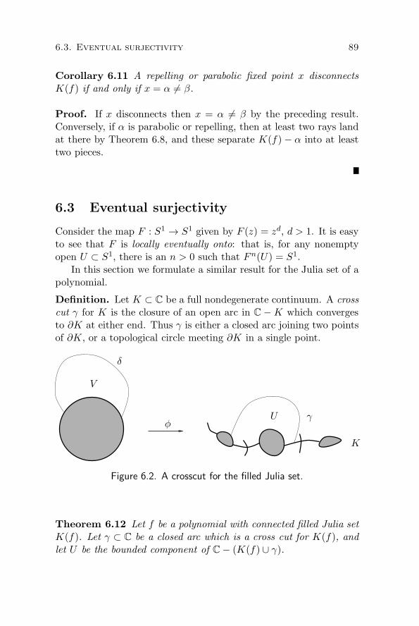
6.3. Eventual surjectivity 89
Corollary 6.11 A repelling or parabolic fixed point x disconnectsK(f) if and only if x = α = β.
Proof. If x disconnects then x = α = β by the preceding result.Conversely, if α is parabolic or repelling, then at least two rays landat there by Theorem 6.8, and these separate K(f)− α into at leasttwo pieces.
6.3 Eventual surjectivity
Consider the map F : S1 → S1 given by F (z) = zd, d > 1. It is easyto see that F is locally eventually onto: that is, for any nonemptyopen U ⊂ S1, there is an n > 0 such that Fn(U) = S1.
In this section we formulate a similar result for the Julia set of apolynomial.
Definition. Let K ⊂ C be a full nondegenerate continuum. A crosscut γ for K is the closure of an open arc in C −K which convergesto ∂K at either end. Thus γ is either a closed arc joining two pointsof ∂K, or a topological circle meeting ∂K in a single point.
φγU
K
δ
V
Figure 6.2. A crosscut for the filled Julia set.
Theorem 6.12 Let f be a polynomial with connected filled Julia setK(f). Let γ ⊂ C be a closed arc which is a cross cut for K(f), andlet U be the bounded component of C− (K(f) ∪ γ).

90 Chapter 6. Polynomials and external rays
Then there exists an integer n > 0 such that the Julia set of f iscontained in the bounded component of C− fn(U).
Proof. Let φ : (C − ∆) → (C − K(f)) be the Riemann mappingnormalized as before.
Suppose γ joins z1 and z2, two distinct points in ∂K. Let δ =φ−1(γ) and let V = φ−1(U). By Corollary 6.4, the ends of δ convergeto points t1 and t2 on S1, and the corresponding external rays landat z1 and z2; thus t1 = t2. Consequently V contains an open intervalon S1. (See Figure 6.2.)
Therefore S1 ⊂ Fn(V ) for some n > 0, where F (z) = zd. SinceFn(V ) is open, it contains a simple closed curve separating S1 frominfinity, so fn(U) disconnects the Julia set from infinity.
Here is an application that will be used repeatedly in our studyof the combinatorics of renormalization (§7).
Theorem 6.13 (Connectedness principle) Let f : C → C be apolynomial with connected filled Julia set K(f). Let fn : U → V bea polynomial-like map of degree d > 1 with connected filled Julia setKn. Then:
1. The Julia set of fn : U → V is contained in the Julia set of f .
2. For any closed connected set L ⊂ K(f), L ∩ Kn is also con-nected.
Proof. The first claim is immediate from the fact that repellingperiodic points of fn are dense in the Julia set of fn : U → V . Thisfollows from the fact that fn is hybrid equivalent to a polynomial(Theorem 5.7).
For the second, suppose L∩Kn is not connected. Then there is abounded component W of C−(L∪Kn) such that L∩∂W is a propersubset of ∂W (see Figure 6.3). Therefore we can construct an arc γin W forming a cross cut for Kn. This cross cut can be chosen to liearbitrarily close to Kn.

6.4. Laminations 91
Kn
L
W
Figure 6.3. Proof of connectedness.
By Theorem 5.7, fn is topologically conjugate to a polynomial ofdegree d near Kn. Using Theorem 6.12, we conclude that the regionU between γ and Kn eventually maps onto an open set separatingKn from infinity. Since U ⊂ W ⊂ K(f) and the filled Julia set K(f)is full, we conclude that Kn lies in the interior of K(f). But this isimpossible, since ∂Kn ⊂ ∂K(f). Thus L ∩Kn is connected.
6.4 Laminations
A point in the Julia set of a polynomial can be the landing pointof more than one external ray. Knowledge of the coincidence ofexternal rays goes a long way towards determining the combinatoricsof the polynomial. These coincidences are conveniently encoded bya lamination.
In this section we define the rational lamination of a polynomialwith connected Julia set, and give a topological criterion for rationalrays to land at the same point. This criterion will be used in theAppendix on quotient maps.
The theory of laminations is implicit in work of Douady and Hub-bard and explicitly developed in [Th2]. Some authors use a different

92 Chapter 6. Polynomials and external rays
but closely related definition of lamination, emphasizing chords ofthe circle rather than equivalence classes.
Let S1 = R/Z, and identify S1 with the boundary of the unitdisk ∆ via the map t +→ exp(2πit).
Definitions. A lamination λ ⊂ S1 × S1 is an equivalence relationon circle such that the convex hulls of distinct equivalence classesare disjoint. One may form the convex hull of an equivalence classusing either the Euclidean or hyperbolic metric on ∆; the results arehomeomorphic. Indeed, the former corresponds to the Klein modelfor the hyperbolic plane.
The support of a lamination is the union of its nontrivial equiv-alence classes (those classes consisting of more than one point). Alamination is finite if its support is a finite set.
Let f be a monic polynomial with connected Julia set. The ra-tional lamination λQ(f) is defined by t ∼ t′ if t = t′, or if t and t′
are rational and the external rays Rt and Rt′ land at the same pointin the Julia set J(f). It is easy to verify that λQ(f) is a lamination,using the fact that two simple closed curves on the sphere cannotcross at just one point.
Now let λ be a finite lamination with support Θ. We will give acondition which implies λ ⊂ λQ(f).
Letφ : (C−∆) → (C−K(f))
denote the Riemann mapping with φ(z)/z → 1 as in §6.2. For t ∈R/Z, let St = [1,∞) exp(2πit).
A λ-ray system is a continuous map
σ :⋃
t∈Θ
St → (C − P (f))
such that:
1. there is an R such that σ(z) = φ(z) when |z| > R, and
2. σ(z) = σ(z′) if and only if z = z′ or |z| = |z′| = 1 and thecorresponding angles t and t′ are equivalent under λ.
Thus σ gives an embedding of the quotient of⋃
Θ St by the equiv-alence relation λ determines on the endpoints of the St’s.

6.4. Laminations 93
Two λ-ray systems σ0 and σ1 are homotopic if there is a contin-uous family of λ-ray systems σs, s ∈ [0, 1] connecting them, and anR independent of s with σs(z) = φ(z) for |z| > R.
A λ-ray system σ0 is invariant if there is a λ-ray system σ1 ho-motopic to σ0 such that
σ0(zd) = f(σ1(z)).
The map σ1 can be viewed as a lifting of σ0(zd). Since f : (C −f−1P (f)) → (C − P (f)) is a covering map, invariance depends onlyon the homotopy class of σ0.
σ
RtSt
x
Figure 6.4. An invariant ray system.
Example. Let x be a fixed point of f lying outside the postcriticalset P (f), and supposeRt lands at x for all t ∈ Θ ⊂ R/Z, |Θ| > 1. Letλ be the equivalence relation with the single nontrivial equivalenceclass Θ. Define σ on
⋃Θ St by σ(z) = φ(z) for |z| > 1 and σ(z) = x
when |z| = 1. Then σ is an f -invariant λ-ray system; see Figure 6.4.
Theorem 6.14 If f admits an invariant λ-ray system, then λ is asubset of the rational lamination of f .
We will need:
Theorem 6.15 Let f be a polynomial of degree d > 1. Then exactlyone of the following holds:
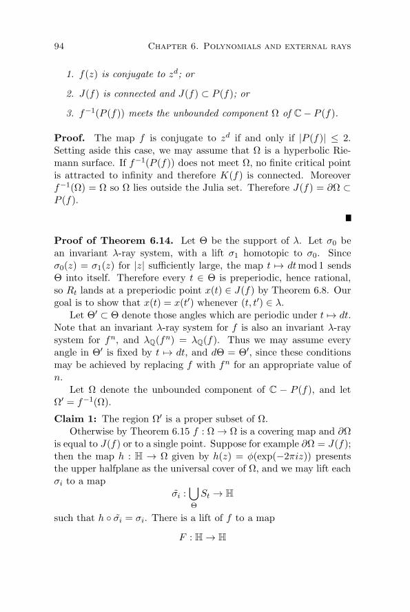
94 Chapter 6. Polynomials and external rays
1. f(z) is conjugate to zd; or
2. J(f) is connected and J(f) ⊂ P (f); or
3. f−1(P (f)) meets the unbounded component Ω of C− P (f).
Proof. The map f is conjugate to zd if and only if |P (f)| ≤ 2.Setting aside this case, we may assume that Ω is a hyperbolic Rie-mann surface. If f−1(P (f)) does not meet Ω, no finite critical pointis attracted to infinity and therefore K(f) is connected. Moreoverf−1(Ω) = Ω so Ω lies outside the Julia set. Therefore J(f) = ∂Ω ⊂P (f).
Proof of Theorem 6.14. Let Θ be the support of λ. Let σ0 bean invariant λ-ray system, with a lift σ1 homotopic to σ0. Sinceσ0(z) = σ1(z) for |z| sufficiently large, the map t +→ dtmod1 sendsΘ into itself. Therefore every t ∈ Θ is preperiodic, hence rational,so Rt lands at a preperiodic point x(t) ∈ J(f) by Theorem 6.8. Ourgoal is to show that x(t) = x(t′) whenever (t, t′) ∈ λ.
Let Θ′ ⊂ Θ denote those angles which are periodic under t +→ dt.Note that an invariant λ-ray system for f is also an invariant λ-raysystem for fn, and λQ(fn) = λQ(f). Thus we may assume everyangle in Θ′ is fixed by t +→ dt, and dΘ = Θ′, since these conditionsmay be achieved by replacing f with fn for an appropriate value ofn.
Let Ω denote the unbounded component of C − P (f), and letΩ′ = f−1(Ω).
Claim 1: The region Ω′ is a proper subset of Ω.Otherwise by Theorem 6.15 f : Ω → Ω is a covering map and ∂Ω
is equal to J(f) or to a single point. Suppose for example ∂Ω = J(f);then the map h : H → Ω given by h(z) = φ(exp(−2πiz)) presentsthe upper halfplane as the universal cover of Ω, and we may lift eachσi to a map
σi :⋃
Θ
St → H
such that h σi = σi. There is a lift of f to a map
F : H → H

6.4. Laminations 95
of the form F (z) = dz + k for some integer k, for which
σ0(zd) = F (σ1(z)).
But for |z| sufficiently large the mappings σi coincide and send eachSt to a vertical line in the upper halfplane. Since only one vertical lineis invariant under F while |Θ| > 1, we obtain a contradiction. Theargument when f(z) is conjugate to zd is similar. This establishesClaim 1.
Now by invariance we may construct a sequence of λ-ray systemsσn such that σn(zd) = f(σn+1(z)). Assume σ0(z) = φ(z) for |z| >R > 1; then σn(z) = φ(z) when |z| > Rn = R1/dn → 1 as n → ∞.In other words, for n large σn carries most of St onto most of theexternal ray Rt.
For t ∈ Θ, let
Fn,t = St ∩ z : |z| ≤ Rn.
Let En,t denote the Euclidean diameter of σn(Fn,t).
Claim 2: As n → ∞, En,t → 0.To establish this claim, first assume t ∈ Θ′, so dt = t. Let ρ(z)|dz|
denote the hyperbolic metric on Ω, and let
Hn,t =∫
Fn,t
ρ(σn(z))|σ′n(z)||dz|
denote the parameterized hyperbolic length of the image of Fn,t.Since f : Ω′ → Ω is a covering map, and σn+1 is a lift of σn, thelength of image of Fn+1,t relative to the hyperbolic metric on Ω′ isequal to Hn,t. Since Ω′ is a proper subset of Ω and inclusions arecontracting, we have Hn+1,t ≤ Hn,t. Moreover the contraction of theinclusion Ω′ → Ω is uniform on any compact subset of Ω′, so eitherHn,t → 0 or σn(Fn,t) eventually leaves every compact subset of Ω.In the former case the Euclidean diameter En,t → 0 because thehyperbolic length bounds the Euclidean length. In the latter caseσn(Fn,t) tends to the boundary of Ω, so its Euclidean diameter tendsto zero because the ratio of the hyperbolic to Euclidean metric tendsto infinity (cf. Theorem 2.3).
This establishes Claim 2 when t ∈ Θ′. Now for any t ∈ Θ,
f(σn+1(Fn+1,t)) = σn(Fn,dt),

96 Chapter 6. Polynomials and external rays
and dt ∈ Θ′, so the Euclidean diameter of the image of Fn,t tends tozero in this case as well (because Fn+t,t is connected).
Finally we show Claim 2 implies the theorem. Indeed,
σn(Rn exp(2πit)) = φ(Rn exp(2πit)) → x(t)
as n → ∞. On the other hand, whenever (t, t′) ∈ λ,
σn(Fn,t) ∪ σn(Fn,t′)
is a connected set of Euclidean diameter at most
En,t + En,t′ → 0
containing σn(Rn exp(2πit)) to σn(Rn exp(2πit′)). Thus x(t) = x(t′)as desired.

Chapter 7
Renormalization
Renormalization is a tool for the study of nonlinear systems whoseessential form is repeated at infinitely many scales.
For a quadratic polynomial f(z) = z2 + c, this repetition of formtakes place when a high iterate fn sends a small neighborhood ofthe critical point z = 0 over itself by degree two. Then a suitablerestriction of fn is quadratic-like, and we can hope to reduce theanalysis of f to that of its iterate fn. This reduction works bestwhen the quadratic-like map has connected Julia set (so the criticalpoint does not escape). The passage from the quadratic map f tothe quadratic-like map fn is an instance of renormalization.
This chapter develops the combinatorics of renormalization forquadratic polynomials. We begin by showing that when it exists,a renormalization of fn is essentially unique. Then we study then small Julia sets associated to fn, and how they fit together as nvaries. Using this combinatorics we define simple renormalization,which will be our main focus in the sequel. The chapter concludeswith some examples of renormalizable quadratic polynomials.
7.1 Quadratic polynomials
Definitions. Let f(z) = z2 + c be a quadratic polynomial withconnected Julia set. A quadratic-like map is a polynomial-like mapof degree two.
The map fn is renormalizable if there are open disks U and V in
97

98 Chapter 7. Renormalization
C such that the critical point 0 ∈ U and
fn : U → V
is a quadratic-like map with connected Julia set. (Equivalently,fnk(0) ∈ U for all k ≥ 0.) 1
The choice of a pair (U, V ) as above is a renormalization of fn.Let
R(f) = n ≥ 1 : fn is renormalizable.
The integers n which appear inR(f) are the levels of renormalization.
Theorem 7.1 (Uniqueness of renormalization) Any two renor-malizations of fn have the same filled Julia set.
Proof. Let fn : U1 → V 1 and fn : U2 → V 2 be two renormal-izations of fn, with filled Julia sets K1 and K2. By Theorem 6.13,L = K1 ∩ K2 is connected, and clearly fn(L) = L. Let U be thecomponent of U1∩U2 containing L, and let V = fn(U). By Theorem5.11, fn : U → V is polynomial-like with filled Julia set equal to L,and of degree two because the critical point z = 0 lies in L. Sincethe degrees of all three maps are the same, we have L = K1 = K2.
Next we collect together notation that will be used in the sequel.Suppose for each n in R(f) we have chosen a renormalization
fn : Un → Vn.
Then:
• Pn, Jn and Kn denote the postcritical set, Julia set and filledJulia set of the quadratic-like map fn : Un → Vn. By assump-tion Jn and Kn are connected, so Pn ⊂ Kn.
1Milnor has suggested the following notation. Let f be a polynomial witha distinguished critical point ω. Then f is n-renormalizable about ω if thereare open disks U and V containing ω such that fn : U → V is polynomial-likewith connected Julia set, and ω is the only critical point of f in U . Thus ourterminology “fn is renormalizable” is shorthand for “fn is 1-renormalizable aboutω = 0.”

7.1. Quadratic polynomials 99
• Kn(i) = f i(Kn) for i = 1, . . . , n. These small filled Julia setsare cyclically permuted by f . Note that Kn(n) = Kn.
• Pn(i) = Kn(i) ∩ P (f) is the ith small postcritical set. We haveP (f) = ∞ ∪
⋃ni=1 Pn(i).
• Jn(i) = ∂Kn(i) is the ith small Julia set.
• Kn = Kn(1) ∪ . . . ∪ Kn(n) is the union of the small filledJulia sets at level n. We have f(Kn) = Kn.
• Jn = Jn(1) ∪ . . . ∪ Jn(n).
• Vn(i) = f i(Un) for i = 1, . . . , n. Then the quadratic-like mapfn is factored as
Unf−→ Vn(1)
f−→ . . .f−→ Vn(n) = Vn,
where the first map Un → Vn(1) is proper of degree two andthe remaining maps are univalent.
• Un(i) is the component of f i−n(Un) contained in Vn(i). We willsee that fn : U(i) → V (i) is quadratic-like (Theorem 7.2).
• P ′n(i), J
′n(i) and K ′
n(i) are defined by P ′n(i) = −Pn(i), and so
on. Each primed object has the same image under f as itsunprimed companion, and for i = n the primed and unprimedobjects are disjoint.
By Theorem 7.1, the filled Julia set Kn of a renormalization iscanonical, even though the choice of Un and Vn may not be. As aconsequence, Kn(i), Jn(i), Pn(i) and their primed companions arealso canonical.
Next we investigate the deployment of the small filled Julia setsKn(1), . . . Kn(n).
Theorem 7.2 Let fn be renormalizable. Then for i = 1, . . . , n,
fn : Un(i) → Vn(i)
is quadratic-like with filled Julia set Kn(i). Similarly,
(−fn) : U ′n(i) → V ′
n(i)

100 Chapter 7. Renormalization
is quadratic-like with filled Julia set K ′n(i). Both maps are holomor-
phically conjugate to fn : Un → Vn.
Proof. The map fn−i : Vn(i) → Vn(n) is univalent, and it conju-gates fn : Un(i) → Vn(i) to fn : Un → Vn, which is quadratic-like.Therefore fn : Un(i) → Vn(i) is quadratic-like, and its filled Julia setisKn(i) because fn−i(Kn(i)) = Kn. Similarly, (−fn−i) : U ′
n(i) → Un
conjugates fn to (−fn) because f(−z) = f(z).
Kn(j)Kn(i)
E
Figure 7.1. The small Julia sets are almost disjoint.
Theorem 7.3 (Almost disjoint Julia sets) Suppose two distinctsmall filled Julia sets Kn(i) and Kn(j) have a nonempty intersection.Then Kn(i) ∩Kn(j) = x, where x is a repelling fixed point of fn.
Proof. Let E = Kn(i)∩Kn(j). Then fn(E) ⊂ E and E is connectedby Theorem 6.13.
LetW be the component of Un(i)∩Un(j) containing E (see Figure7.1), and let W ′ = fn(W ). By Theorem 5.11, fn : W → W ′ ispolynomial-like, and of degree one because Kn(i) = Kn(j). By theSchwarz lemma, E consists of a single repelling fixed point for fn.

7.1. Quadratic polynomials 101
Theorem 7.4 Suppose fn is renormalizable. Then any attracting orindifferent periodic point and any periodic component of the interiorof K(f) is contained in Kn(i) for a unique i. Its period is divisibleby n.
Corollary 7.5 Every periodic point of f with period less than n isrepelling.
Proof. Let x be an attracting periodic point, or an indifferent peri-odic point lying in the Julia set. Then x lies in P (f) by basic factsin rational dynamics (Corollary 3.7). Therefore x ∈ Kn(i) for somei. The small filled Julia sets meet only at repelling points, if at all(Theorem 7.3), so this i is unique. By uniqueness, if fp(x) = x thenfp(Kn(i)) = Kn(i), and therefore the period p is a multiple of n.
If D is a component of the interior of K(f) of period p, then D isan attracting or parabolic basin, or a Siegel disk. In the attractingor parabolic case, D is contained in the unique Kn(i) containing thecorresponding attracting or parabolic periodic point. If D is a Siegeldisk, then ∂D ⊂ P (f), and thus Pn(i) ∩ ∂D is open and nonemptyin ∂D for some i. Since Pn(i) is invariant under fnp and fnp|Dis an irrational rotation, it is easy to see that ∂D ⊂ Pn(i). ThenD ⊂ Kn(i) because Kn(i) is full, and this i is unique because theinteriors of the small filled Julia sets are disjoint. Uniqueness againimplies n|p.
An indifferent periodic point in the interior of K(f) is the centerof a unique Siegel disk, so this case is also covered.
Theorem 7.6 (Least common renormalization) If fa and f b arerenormalizable, then so is f c, where c is the least common multipleof a and b. The corresponding filled Julia sets satisfy Kc = Ka ∩Kb.
Proof. Define U∗a by
U∗a = z ∈ Ua : faj(z) ∈ Ua for j = 1, . . . c/a − 1;
then f c : U∗a → Va is polynomial-like of degree 2c/a. Define U∗
b in thesame way, with b in place of a.

102 Chapter 7. Renormalization
By Theorem 6.13, the set L = Ka ∩Kb is connected. Let Uc bethe component of U∗
a ∩ U∗b containing L, and let Vc = f c(Uc). By
Theorem 5.11, the map f c : Uc → Vc is polynomial-like, with filledJulia set L.
The critical point z = 0 lies in f i(L) = f i(Ka) ∩ f i(Kb) if andonly if a|i and b|i; that is, i must be a multiple of c. Therefore f c hasa single critical point in L, and since L is connected, f c : Uc → Vc
is polynomial-like of degree 2. Therefore c ∈ R(f) and Kc = L =Ka ∩Kb.
Corollary 7.7 If fa and f b are renormalizable, and a divides b, thenKa ⊃ Kb.
7.2 Small Julia sets meeting at periodic points
The combinatorics of renormalization is simplest when the small Ju-lia sets are actually disjoint. We have seen, however, that the smallJulia sets can touch at repelling periodic points. In this section wewill show that the periods of these touching points tend to infinityas the level of renormalization tends to infinity.
Theorem 7.8 (High periods) Given a period p, there are onlyfinitely many n in R(f) such that the small filled Julia set Kn con-tains a periodic point of f of period p.
Theorem 7.8 is often a good substitute for disjointness. The mainpoint in the proof is to show that for n ∈ R(f) sufficiently large, Kn
does not contain either fixed point of f .To begin an analysis of fixed points, let f(z) = z2 + c be a
quadratic polynomial with connected Julia set such that both fixedpoints α and β of f are repelling.
Theorem 7.9 The external rays landing at α are permuted transi-tively by f . The external rays landing at −α separate β from thecritical point of f .

7.2. Small Julia sets meeting at periodic points 103
Proof. By Theorem 6.8, a finite number q of external rays landat the α fixed point of f . If a ray Rt lands at α, then so doesf(Rt) = R2t; since f is locally injective at α, it is clear that fpermutes the rays landing there. We will show this permutation istransitive.
The rays landing at α are forward invariant, and they divide thecomplex plane into q open components P1, . . . , Pq; we may assume Pq
contains the critical point and −α. The preimages of these rays landat α and −α, dividing the plane into 2q − 1 pieces Q1, Q2, . . . Q2q−1.Since only the piece Pq is subdivided by the rays landing at −α, wemay label these new pieces so Qi = Pi for 1 ≤ i < q and Qq ⊂ Pq
contains the critical point. (See Figure 7.2.)Assume i < q, so Pi = Qi does not contain the critical point.
Then f maps Pi univalently to another piece f(Pi) = Pj . The an-gle between the rays bounding f(Pi) is twice the angle between therays bounding Pi. Since the angle cannot increase without bound,eventually Pi maps onto Pq. Therefore the rays landing at α arepermuted transitively.
Since β is fixed by f while f(Pi) is disjoint from Pi when i < q, itfollows that β is contained in Pq. Similarly β is not contained in Qq,since f(Qq) = Pi for some i < q (containing the critical value). Thusβ is contained in Qj for some j > q, and therefore the rays landingat −α separate β from the critical point in Qq.
Remark. The preceding argument contains the beginnings of theYoccoz puzzle, discussed more fully in §8.2.
We now consider f(z) = z2+ c such that fn is renormalizable forsome n > 1. Then the Julia set of f is connected, and by Corollary7.5 f has two repelling fixed points α and β. (In other words, the c’sfor which a proper iterate of z2 + c is renormalizable lie outside themain cardioid of the Mandelbrot set.)
Theorem 7.10 If fn is renormalizable and n > 1, then the smallfilled Julia set Kn does not contain the β fixed point of f .
Proof. Suppose to the contrary that Kn contains β. Then f(Kn) =Kn(1) also contains β, since f(β) = β. By Theorem 7.3, the small

104 Chapter 7. Renormalization
−β
−αα
f
α −α
β
β
Figure 7.2. Rays landing at α and β.

7.2. Small Julia sets meeting at periodic points 105
filled Julia sets meet in at most one point, so Kn does not contain α.Consequently Kn does not contain −α either. Thus Kn is disjointfrom the rays landing at −α. But these rays separate the criticalpoint from β, which is impossible because Kn is connected and con-tains both these points.
Theorem 7.11 Suppose fn is renormalizable for n > 1, and α ∈Kn. Let ρ be the number of components of Kn − α. Then
nρ ≤ q,
where q is the number of external rays landing at α.
Combining the last two results, we obtain:
Corollary 7.12 For n ∈ R(f), n > q, the small filled Julia set Kn
does not contain any fixed point of f .
The idea of the proof of the Theorem 7.11 is straightforward: theset Kn is separated into nρ components by α, and these componentsare locally cyclically permuted by f . So starting with a single exter-nal ray landing at α, we obtain nρ such rays by applying f to it. Wewill use Riemann mappings and Lindelof’s theorem to formalize thisargument.
Proof of Theorem 7.11. Let
Θ = t1, . . . tq ⊂ R/Z
denote the external angles of the rays landing at the α fixed pointof f . By Theorem 7.9, f permutes these rays transitively; in otherwords, the map t +→ 2tmod 1 gives a cyclic permutation of Θ. LetF : Θ → Θ denote the inverse of this permutation.
The map F can be described geometrically as follows: startingwith a ray Rt landing at α, form the set f−1(Rt); this consists ofone ray Rs landing at α, and another Rs+1/2 landing at −α. ThenF (t) = s.

106 Chapter 7. Renormalization
Recall Kn =⋃n
i=1Kn(i) is the union of the small Julia sets atlevel n. Let Ln = f−1(Kn).
Both Kn and Ln are full continua. Indeed, Kn is a fan of n copiesof Kn joined at α, and
Ln = Kn ∪ −Kn(1) ∪ . . . ∪ −Kn(n− 1)
is obtained from Kn by attaching n− 1 copies of Kn to it at −α.For appropriate Riemann mappings πL and πK we obtain a com-
mutative diagram of conformal coverings maps:
C−∆z2−−−→ C−∆
πL
3 πK
3
C− Lnf−−−→ C−Kn.
We will denote external rays for the Riemann mapping πK by R′t;
thus
R′t = πK((1,∞) exp(2πit)).
Since α separates Kn into ρ components, it also separates eachKn(i) into ρ pieces; thus Kn − α has exactly nρ components. ByTheorem 6.6, there are exactly nρ external rays of the form R′
t land-ing at α under the Riemann mapping πK; denote their external anglesby Θ′ ⊂ R/Z.
Define a map F ′ : Θ′ → Θ′ as follows. Given an external ray R′t
landing at α under the Riemann mapping πK, consider its inverseimage f−1(R′
t). This set consists of two paths γ and −γ landing atα and −α respectively. The path γ lies outside Ln and hence outsideKn. By Lindelof’s theorem (that is, Corollary 6.4), π−1
K (γ) convergesto a point z = exp(2πis) on the unit circle and the external ray R′
s
lands at α. Set F ′(t) = s.Finally, define h : Θ → Θ′ by a similar construction: given an
external ray Rt in the complement of the filled Julia set K(f), leth(t) = t′ where π−1
K (Rt) terminates at exp(2πit′).The conclusion of the argument amounts to verifying:
(1) h gives a semiconjugacy between F and F ′; that is,

7.2. Small Julia sets meeting at periodic points 107
the diagram
ΘF−−−→ Θ
h
3 h
3
Θ′ F ′
−−−→ Θ′
is commutative; and
(2) F ′ is a cyclic permutation of Θ′.
Indeed, (1) and (2) imply h is surjective, so |Θ| ≥ |Θ′| which sayssimply that q ≥ nρ.
Proof of (1). Let t ∈ Θ. Then Rt and R′h(t) both land at α. In
addition, the preimages of Rt and R′h(t) under πK land at the same
point on the unit circle — namely exp(2πih(t)).The external ray RF (t) is the unique component of the preimage
of Rt under f which terminates at α. Similarly, there is a uniquecomponent γ of the preimage of R′
h(t) which also terminates at α.
Since f πL(z) = πK(z2), we can construct RF (t) by first liftingRt via πK, then choosing the appropriate component of its preimageunder z2, and then projecting by πL. Note that the other componentof the preimage projects by πL to a ray landing at −α.
The same considerations apply to the construction of γ fromR′
h(t). Since γ and RF (t) both terminate at α (rather than −α), andtheir lifts by πK land at the same point on S1, the correct furtherpreimages under z2 also land at the same point on S1. Equivalently,π−1L (γ) and π−1
L (RF (t)) land at the same point w ∈ S1. See Figure7.3, which depicts an example in which n = ρ = 2.
Now let i : (C − Ln) → (C − Kn) denote the inclusion mapping,and let i denote its lift to the uniformizations of the domain andrange by πL and πK respectively. The image of i is C − (∆ ∪ E),where E = π−1
K (Ln).Since Ln − Kn is cut off from Kn by finitely many rays landing
at −α, while γ and RF (t) land at α, we have i(w) ∈ E. By Schwarz
reflection, i extends continuously to a neighborhood of w. Thus theimages of γ and RF (t) under i π−1
L land at the same point on thecircle.
Equivalently, the preimages of RF (t) and of γ under πK terminateat the same place. By definition, the form preimage terminates at

108 Chapter 7. Renormalization
h(F (t)), while the latter terminates at F ′(h(t)). Thus F ′(h(t)) =h(F (t)).
w
πK πL πK
γ
RF (t)
α −αα α
E
f
z2
i
i
RtR′h(t)RF (t)
γ
C−KnC−Kn C− Ln
Figure 7.3. Factoring Riemann mappings.
Proof of (2). The rays R′t for t ∈ Θ′ divide the set Kn−α into its
nρ components, P1, . . . , Pnρ. We may assume the critical point liesin P1. Arguing as in Theorem 7.9, one may show that for each i > 1,f(Pi) = Pj for some j, and if f(Pi) lies in the sector bounded byrays R′
s and R′t, then Pi lies in the sector bounded by rays R′
F (s) and
R′F (t). This reduces the proof to checking that each Pi eventually
maps onto P1.We know P1 ⊂ Kn and each Pi ⊂ Kn(j) for some j, 1 ≤ j ≤ n.
Thus fn−j(Pi) ⊂ Kn, so it suffices to verify the claim when Pi ⊂Kn. Consider the polynomial g which is hybrid equivalent to thepolynomial-like map fn : Un → Vn. If α corresponds to the β fixedpoint of g, then Kn − α has only one component so we are done.Otherwise the α fixed point of f corresponds to the α fixed point ofg. Then the desired result follows from the assertion that g cyclicallypermutes the rays landing at its α fixed point (Theorem 7.9).

7.3. Simple renormalization 109
Proof of Theorem 7.8 (High periods). Let w be a point of periodp for f . We will show w ∈ Kn for only finitely many n ∈ R(f).
Suppose there is an a in R(f) with a > p and w ∈ Ka; thenfp(w) = w ∈ Ka(p). By Theorem 7.3, w = Ka(p) ∩ Ka and wis a repelling fixed point of fa. Let g be the quadratic polynomialto which fa : Ua → Va is hybrid equivalent. Then w corresponds toeither the α or β fixed point of g.
First suppose w corresponds to β. We claim w ∈ Kb for all b > ain R(f). Indeed, Theorem 7.6 guarantees that f c is renormalizableand Kc = Kb ∩ Ka where c = lcm(a, b). The renormalization off c provides a renormalization of gc/a whose filled Julia set does notcontain the β fixed point of g, by Theorem 7.10. It follows that Kc,and therefore Kb, fails to contain w.
Now suppose w corresponds to the α fixed point of g. Let q bethe number of external rays for g landing at its α fixed pont. ByCorollary 7.12, α is disjoint from the filled Julia set of any renormal-ization of g of level greater that q. So the same reasoning shows Kb
fails to contain w for any b > qa.Thus the set of n ∈ R(f) such that w ∈ Kn is finite. Since
there are only finitely many periodic points of period p, the theoremfollows.
7.3 Simple renormalization
In this section we introduce some terminology and numerical invari-ants for renormalization. In particular we define simple renormaliza-tion, which plays a fundamental role in the sequel.
Definitions. Let f(z) = z2 + c be a quadratic polynomial, andlet n belong to R(f). For 1 ≤ i ≤ n, fn : Un(i) → Vn(i) is apolynomial-like map, hybrid equivalent to a quadratic polynomialg with connected Julia set. The fixed points of g may be labeledα and β in accordance with §6.2. Let αn(i) and βn(i) denote thecorresponding fixed points in Kn(i).

110 Chapter 7. Renormalization
By Theorem 7.3 if two small Julia sets meet, say Kn(i)∩Kn(j) =p for i = j, then p = αn(i) or p = βn(i) (but not both – since p isa repelling fixed point of fn, αn(i) = βn(i)).
Theorem 7.13 (Same type) All intersections of small Julia setsat a given level n occur at the same type of fixed point (α or β).
A more precise statement of Theorem 7.13 is the following: it isnever the case that Kn(i)∩Kn(j) = αn(i) while Kn(i′)∩Kn(j′) =βn(i′).
Proof. First note that f(αn(i)) = αn(i+1) and f(βn(i)) = βn(i+1)(where n+1 is interpreted as 1). For i < n this is immediate from thefact the f gives a conformal conjugacy between fn : Un(i) → Vn(i)and fn : Un(i + 1) → Vn(i + 1). For i = n it follows from the factthat fn fixes αn(n) and βn(n).
Now suppose two small Julia sets meet at αn(j) while two othersmeet at βn(k); we will find a contradiction. Since f cyclically per-mutes the collections Kn(i), αn(i) and βn(i), every point of the formαn(i) or βn(i) belongs to at least two small Julia sets. Thus |F | ≤ nwhere
F =n⋃
i=1
αn(i),βn(i).
Form a graph with one vertex for each point of F and edges e(i)joining αn(i) to βn(i) for i = 1, . . . , n. This graph has no more ver-tices than edges, so it includes at least one cycle < e(i1), . . . , e(ik) >.Since αn(i1) = βn(i1), we have k > 1. Then L = Kn(i2)∪. . .∪Kn(ik)is connected since adjacent sets in the union meet. By Theorem 6.13,L ∩Kn(i1) is also connected. But L ∩Kn(i1) = αn(i1),βn(i1), acontradiction.
Types of renormalization. A renormalization of fn is of:
α-type, if some pair of small Julia sets meet at their αfixed points;
β-type, if some pair meet at their β fixed points; and of
disjoint type, if the small Julia sets are disjoint.

7.3. Simple renormalization 111
By Theorem 7.13, every renormalization is of exactly one of thesetypes.
A renormalization is simple if it is of β-type or disjoint type.Equivalently, whenever two small Julia sets meet, they do so at theirβ fixed points.
A renormalization is crossed if it is not simple. Crossed is syn-onymous with α-type. The terminology is meant to suggest that thesmall Julia sets cross at their α fixed points.
Let
SR(f) = n ∈ R(f) : the renormalization of fn is simple.
Theorem 7.14 If a ∈ R(f) and b ∈ SR(f), then a divides b or bdivides a.
Proof. Let d be the greatest common divisor of a and b. If d =min(a, b) then a|b or b|a and we are done.
Otherwise, d is less than both a and b, so Ka = Ka(d) andKb = Kb(d). Note that Ka meets Kb because they both containthe critical point z = 0. Therefore f i(Ka) meets f i(Kb) for anyi > 0. In particular, Ka(d) meets Kb(d).
The sequences of sets f i(Ka) and f i(Kb) are periodic with periodsa and b respectively. Some multiple of b is congruent to dmod a, andvice-versa, so Kb meets Ka(d) and Ka meets Kb(d).
Thus L = Kb ∪ Ka(d) ∪ Kb(d) is connected. By Theorem 6.13,L∩Ka is also connected. Since Ka(d)∩Ka is at most a single point,we conclude (Kb ∪Kb(d)) ∩Ka is connected. As both Kb and Kb(d)meet Ka, connectedness implies Kb ∩Kb(d) ∩Ka is nonempty. Butb ∈ SR(f), so Kb and Kb(d) meet at their β fixed points. Thus theβ fixed point of f b : Ub → Vb lies in Ka ∩Kb.
Let c be the least common multiple of a and b. By Theorem7.6, f c is renormalizable, and Kc = Ka ∩Kb. But then the polyno-mial g to which f b : Ub → Vb is hybrid equivalent admits a properrenormalization whose Julia set contains the β fixed point of g. Thiscontradicts Theorem 7.10.

112 Chapter 7. Renormalization
Corollary 7.15 The set SR(f) is totally ordered with respect to di-vision.
By Corollary 7.7, we have:
Corollary 7.16 The sets Kn form a nested decreasing sequence as nincreases through values in SR(f). Consequently, for any pair a < bin SR(f), each small Julia set at level b is contained in some smallJulia at level a, and the same is true for the small postcritical sets.
The following result will be useful for constructing simple renor-malizations in §8.
Theorem 7.17 Let fa be simply renormalizable, and let g be thequadratic polynomial to which fa : Ua → Va is hybrid equivalent.Suppose gb is simply renormalizable. Then f c is simply renormaliz-able, for c = ab.
Proof. To say g is hybrid equivalent to fa means there is a quasi-conformal map ψ : Wf → Wg conjugating fa to g, where Wf andWg are neighborhoods of Ka and K(g).
Suppose gb : Ub → Vb provides a simple renormalization of g.Replacing Ub and Vb by their preimages under a higher iterate ofgb if necessary, we can assume Ub ⊂ Vb ⊂ Wg. Then (Uc, Vc) =(ψ−1(Ub),ψ−1(Vb)) provides a renormalization of f c, where c = ab.
We must verify that the renormalization of f c is simple; we mayassume b > 1. By Corollary 7.7, Kc ⊂ Ka (this is also clear from theconstruction.) Thus every Kc(i) is contained in some Ka(i′).
Now suppose Kc(i) ∩ Kc(j) = x. We have Kc(i) ⊂ Ka(i′)and Kc(j) ⊂ Ka(j′) for some i′ and j′. If i′ = j′, then x mustbe the β fixed point of Ka(i′) because the renormalization of fa
was simple. But then Kc(i) also contains β, contrary to Theorem7.10. Therefore i′ = j′, and fa : Ka(i′) → Ka(i′) is topologicallyconjugate to g : K(g) → K(g). It follows that Kc(i) − Kc(j) isconnected because the renormalization of gb is simple. Therefore therenormalization of f c is also simple.

7.4. Examples 113
Multiplicity and ramification. If fn is renormalizable, its multi-plicity µn is the number of small filled Julia sets meeting Kn, includ-ing Kn itself. The multiplicity is one if and only if the renormaliza-tion is of disjoint type. It is the same as the number of small filledJulia sets in any component of Kn.
The ramification ρn is the number of components of the set Kn−⋃i =nKn(i). This is the same as the number of components ofKn(j)−⋃i =j Kn(i) for any j.The ramification is one if and only if the renormalization is sim-
ple. In fact, Kn ∩⋃
i =nKn(i) is equal to αn(n), βn(n) or ∅according to whether the renormalization is of α-type, β-type of dis-joint type. For a crossed renormalization, αn(n) is repelling andρn > 1 is the number of components of Kn − αn(n) (which is finiteby Corollary 6.9).
7.4 Examples
To illustrate these results, we present (without proofs) several exam-ples of renormalizable quadratic polynomials.
pics/J3.ps not found
pics/J3R.ps not found
Figure 7.4. The small Julia sets are disjoint.
I. Let f(z) = z2 − 1.772892 . . . satisfy f6(0) = 0. For this map, f3
is renormalizable and its quadratic-like restriction f3 : U3 → V3 ishybrid equivalent to z2 − 1. Its Julia set is depicted in Figure 7.4,with K3(1)∪K3(2)∪K3(3) drawn below. In this case the small Juliasets are disjoint.
II. Let f(z) = z2 − 1.401155 . . . be the Feigenbaum polynomial,illustrated in Figure 7.5; then f2 is renormalizable, and again K2(1)∩K2(2) = x where x is a fixed point of f .
The Feigenbaum polynomial has many special properties withrespect to renormalization; for example, f2n is renormalizable for

114 Chapter 7. Renormalization
pics/J2.ps not found
pics/J2R.ps not found
Figure 7.5. The Feigenbaum map: the small Julia sets touch.
any n > 0, and all such renormalizations are hybrid equivalent tof itself. This map can be described as the limit of the “cascade ofperiod doublings” for z2+c as c decreases along the real axis, startingat zero.
It turns out that the point x shared by K2(1) and K2(2) doesnot belong to P (f); indeed the finite postcritical set is a Cantor seton which f acts injectively without periodic cycles. This absence ofperiodic cycles in P (f) (other than infinity) is a general feature ofinfinitely renormalizable maps, as we will see below.
pics/J1.ps not found pics/J1R.ps not found
Figure 7.6. The small postcritical sets touch.
III. Let f(z) = z2 − 1.54368 . . . satisfy f3(0) = f4(0); then f2 isrenormalizable and hybrid equivalent to z2 − 2.
The Julia set of f appears in Figure 7.6; drawn below it is K2(1)∪K2(2), a pair of intervals meeting at x = f3(0), a fixed point of fwhich is also in the postcritical set. So not only do the small Juliasets meet in this example, the small postcritical sets P2(1) and P2(2)also meet.
IV. A perhaps surprising example is given by f(z) = z2+0.389007 . . .+0.215851i . . . ; for this map, the critical point has periodic six, andf2, f3 and f6 are all renormalizable. This shows the set of n forwhich fn is renormalizable does not have to be totally ordered withrespect to division. (The set of simple renormalizations, however, isso ordered.)

7.4. Examples 115
pics/Per6.full.ps not found
pics/Per6.half.ps not found
pics/Per6.third.ps not found
Figure 7.7. Here f2, f3 and f6 are all renormalizable.
pics/J5.ps not found
Figure 7.8. The small Julia set of f2 is an quasiarc.
The filled Julia set of f is rendered at the top of Figure 7.7. LetB be the closure of the immediate basin of attraction of z = 0; thenthe pictures at the bottom depict
⋃f−2n(B) and
⋃f−3n(B). The
closure of the connected component in black containing zero is K2
at the left, and K3 at the right. The map f2 is hybrid equivalentto the “rabbit” z2 − 0.122561 . . . + 0.744861 . . . , while f3 is hybridequivalent to z2 − 1.
V. Let f(z) = z2 + 0.419643 . . . + 0.606291i . . . ; for this map, f2 isrenormalizable and hybrid equivalent to z2−2, but no higher iterateof f is renormalizable. The Julia set of f appears in Figure 7.8. Thesmall Julia sets J2(1) and J2(2) are a pair of quasiarcs (quasicon-formal images of intervals), running horizontally and vertically andcrossing at the α fixed of f .
These example are classified as follows.
I: R(f) = 1, 3, 6. The renormalization f3 is of disjointtype, while that of f6 is of β-type.
II: R(f) = 1, 2, 4, . . . , 2n, . . . . Each renormalizationf2n is of β-type with multiplicity µ2n = 2.
III: R(f) = 1, 2. The renormalization f2 is of β-typewith multiplicity two.

116 Chapter 7. Renormalization
IV: R(f) = 1, 2, 3, 6. The renormalization f2 is of α-type with multiplicity two and ramification three. Simi-larly f3 is of α-type with µ3 = 2, ρ3 = 2. Finally f6 is ofβ-type with µ6 = 6.
V: R(f) = 1, 2; the renormalization f2 is of α-typewith µ2 = ρ2 = 2.
The renormalizations of f2 and f3 in example IV, and of f2 inexample V, are crossed. The others are simple.
Example V shows that a quadratic polynomial need not admitany simple renormalizations (other than f itself), even when fn isrenormalizable for some n > 1.
Tuning. The “tuning” construction of Douady and Hubbard (un-published) provides many more examples of renormalizable polyno-mials.
Quite informally, the idea of tuning is the following. Start with apolynomial g(z) = z2+c such that the critical point z = 0 is periodicof period p. There is a unique Riemann mapping from the immediatebasin of attraction U of z = 0 to the unit disk ∆ which conjugatesgp(z) to z2. This mapping provides “internal angles” for points inthe boundary of U .
Let h(z) = z2 + c′ be a second polynomial with connected Ju-lia set. Replace U with a copy of K(h), identifying points in ∂Uand points in ∂K(h) whose internal and external angles correspond.Carry out a similar surgery on each component of the interior of thefilled Julia set K(g). The result is a new polynomial f(z) = z2 + c′′,the “tuning” of g by h.
As long as h is not z2 + 1/4, fp is simply renormalizable andfp : Up → Vp is hybrid equivalent to h.
For more details, see [Dou1], [Dou2], [Mil1].It would be interesting to have a parallel systematic construction
of polynomials admitting crossed renormalizations.

Chapter 8
Puzzles and infinite
renormalization
This chapter presents basic facts concerning infinitely renormalizablequadratic polynomials.
The set of parameters c for which z2+c is infinitely renormalizableseems to be quite thin. Nevertheless, these mappings are of centralinterest, both for their internal symmetries and because they are yetto be well-understood. For example, these are the only quadraticpolynomials for which the no invariant line fields conjecture is stillopen.
We begin with properties of such polynomials which follow fromthe material already developed. Then we describe the “Yoccoz puz-zle”, a Markov partition for the Julia set, and use it to show thatan infinitely renormalizable map admits infinitely many simple renor-malizations. Next we summarize fundamental results of Yoccoz, Lyu-bich and Shishikura, showing that a quadratic polynomial which isonly finitely renormalizable carries no invariant line field on its Juliaset. Finally we give a lamination criterion for renormalizability.
8.1 Infinite renormalization
Definition. A quadratic polynomial is infinitely renormalizable iffn is renormalizable for infinitely many positive integers n.
117

118 Chapter 8. Puzzles and infinite renormalization
Theorem 8.1 Let f be infinitely renormalizable. Then:
1. All periodic cycles of f are repelling.
2. The filled Julia set of f has no interior.
3. The intersection⋂
R(f) Jn contains no periodic points.
4. The finite postcritical set P (f)∩C contains no periodic points.
5. For any n ∈ R(f), Pn(i) and Jn(j) are disjoint when i = j.
Proof. Corollary 7.5 states that all cycles of period less than n ∈R(f) are repelling. Since f is infinitely renormalizable, every periodiccycle is repelling. Thus K(f) = J(f) because a nonempty open setin the filled Julia set entails an attracting, parabolic or indifferentcycle.
Let x be a periodic point of f . By Theorem 7.8, the forward orbitof x meets Jn for only finitely many n ∈ R(f). Thus x is disjointfrom Jn for all n sufficiently large, and therefore
⋂Jn contains no
periodic points.Since P (f) ∩ C ⊂
⋂Jn, the postcritical set also contains no pe-
riodic points.For i = j, Jn(i) and Jn(j) can only meet at a periodic point by
Theorem 7.3. Therefore Pn(i) ⊂ Jn(i) is disjoint from Jn(j).
Since the Julia set and filled Julia set are equal in the infinitelyrenormalizable case, we have K(f) = J(f), Kn(i) = Jn(i) and Kn =Jn for all n in R(f). For simplicity we will use only the J notationwhen we consider infinitely renormalizable polynomials.
Theorem 8.2 (Small Julia sets attract) Let f be infinitely renor-malizable. Then for any n in R(f), and for almost every x in theJulia set of f , the forward orbit of x lands in Jn.
Remark. Since Jn =⋃n
1 Jn(i) is forward invariant, once an iterateof x lands there it remains in Jn for all future iterations.

8.2. The Yoccoz jigsaw puzzle 119
Proof. The Julia set of f is not the whole sphere, so d(fk(x), P (f)) →0 as i → ∞ for almost every x in J(f) (by Theorem 3.9). The post-critical set is partitioned into disjoint compact pieces Pn(1), . . . Pn(n) =Pn which are permuted by f . Therefore the forward orbit of x accu-mulates on Pn (as well as every other block of the partition).
For all k sufficiently large, when fk(x) is closer to Pn than to therest of P (f), then so is fk+n(x). Thus there is an iterate fk(x) suchthat d(fk+nj(x), Pn) → 0 as j → ∞. Since Pn is a compact subset ofUn, for j large enough y = fk+nj(x) does not escape from Un underiteration of fn. Therefore y ∈ Jn ⊂ Jn.
8.2 The Yoccoz jigsaw puzzle
In this section we describe a Markov partition for the dynamics ofa quadratic polynomial, introduced by Yoccoz. We will use the lan-guage of tableau, developed earlier by Branner and Hubbard in theirclosely related work on cubic polynomials [BH]. For more details thereader is referred to [Mil3], [BH], [Hub] and [Yoc].
Definitions. Let f(z) = z2 + c be a quadratic polynomial withconnected Julia set and both fixed points repelling. For simplicity,we also assume that the forward orbit of the critical point is disjointfrom the α fixed point of f .
Let φ be the Riemann mapping from C − ∆ to C − K(f), nor-malized so φ′(∞) = 1 as in §6.2. Consider the disk D bounded bythe image of the circle |z| = 2 under φ. This disk encloses K(f)and is cut into q > 1 pieces by the external rays landing at the αfixed point of f (compare §6).
pics/Puz.1.3.ps not found
Figure 8.1. Puzzle pieces for f(z) = z2 − 1.
Following [Mil3], we denote these pieces by P0(c0), . . . , P0(cq−1),where ci = f i(0) and ci lies in P0(ci). They form the “puzzle pieces”

120 Chapter 8. Puzzles and infinite renormalization
of depth zero. Each piece is a closed disk, whose boundary consistsof the α fixed point, segments of external two rays and part of ∂D.
The puzzle pieces at depth d + 1 are defined inductively as thecomponents of f−1(P ), where P ranges over all puzzle pieces at depthd.
The puzzle pieces at depth d have disjoint interiors and cover theJulia set. As the depth increases, the puzzles become successivelyfiner: a piece at depth d+ 1 is contained in a unique piece at depthd.
Example. The first few pieces in the puzzle for f(z) = z2 − 1 aredepicted in Figure 8.1.
Every point z in K(f) which does not lie in the grand orbit ofα is contained in a unique puzzle piece Pd(z) at depth d. ClearlyPd(f(z)) = f(Pd+1(z)). The tableau for z is the array of piecesPd(fk(z)) for d, k ≥ 0; it records the symbolic dynamics of z relativeto the puzzle partitions. (Usually one adds more information to thetableau that will not be needed here.)
The renormalization period. The pieces Pd(fk(0)) = Pd(ck) formthe critical tableau; it is periodic if for some n > 1, Pd(cn) = Pd(0)for all depths d. The least such n is the period of the critical tableau.Since the pieces P0(0), . . . P0(cq−1) are always distinct, the periodmust be greater than one.
Similarly, we define the renormalization period of f to be the leastn > 1 such that fn is simply renormalizable.
By convention, if the tableau is aperiodic or if f has no propersimple renormalizations, we define the corresponding period to be∞.
Theorem 8.3 Let f be a quadratic polynomial with connected Juliaset and both fixed points repelling, such that the forward orbit of thecritical point avoids the α fixed point of f .
Then the period of the critical tableau Pd(ck) is equal to the renor-malization period of f .
Proof. Let n > 1 be the period of the critical tableau, assumed tobe finite. We will first show that fn is simply renormalizable, so nis greater than or equal to the renormalization period of f .

8.2. The Yoccoz jigsaw puzzle 121
Since the period is exactly n, for d large enough the pieces Pd(c1),. . . , Pd(cn−1) have interiors disjoint from Pd(0). Therefore fn :Pd+n(0) → Pd(0) is a proper map of degree two.
Now by slightly thickening these pieces, one obtains a quadratic-like map with connected Julia set (see [Mil3, Lemma 2] for details).
We must check that the renormalization is simple. The smallfilled Julia set Kn is contained in Pd+n(c0), so Kn(i) is containedin Pd+n−i(ci). By our choice of d these puzzle pieces have disjointinteriors for i = 1, . . . , n. Two puzzle pieces whose interiors aredisjoint can only meet at a point in the grand orbit of α. On theother hand, Kn(i) and Kn(j) can only meet at a repelling fixed pointof fn. Thus Kn(i) and Kn(j) can only touch at α. If they do, thensince f(α) = α, all the small filled Julia sets meet at α and n = q,the number of external rays landing at α.
By Theorem 7.11, nρn ≤ q, where ρn is the ramification of fn
(which in this case is equal to the number of components ofKn−α).Since n = q, the ramification ρn = 1 and therefore fn is simplyrenormalizable.
Now suppose fn is simply renormalizable, for n > 1. To completethe proof, we will show that the period of the critical tableau is lessthan or equal to n.
First note that Kn is contained in P0(0). This is clear if Kn doesnot contain α. If Kn meets α, then so does Kn(1), and thus α isthe β fixed point of Kn (by our assumption of simplicity). ThereforeKn − α is connected, so it lies in single component of K(f) − α,and consequently Kn ⊂ P0(0).
Next we claim Kn ⊂ Pd(0) for all depths d. Indeed, Kn is con-nected, so for any k > 0 the set f−kn(Kn) has a unique componentcontaining Kn. Thus Kn is contained in a unique puzzle piece atdepth kn, which must coincide with Pkn(0) because 0 ∈ Kn. For anyd we can choose k so kn > d, from which it follows that Kn ⊂ Pd(0).
On the other hand, cn = fn(0) ∈ Kn as well, so Pd(cn) = Pd(0)for all d. Therefore the critical tableau has period less than or equalto n.
Remark. When the critical tableau has period n, one has Pd(ci+n) =Pd(ci) for all i and d; see [Mil3, Lemma 2]).
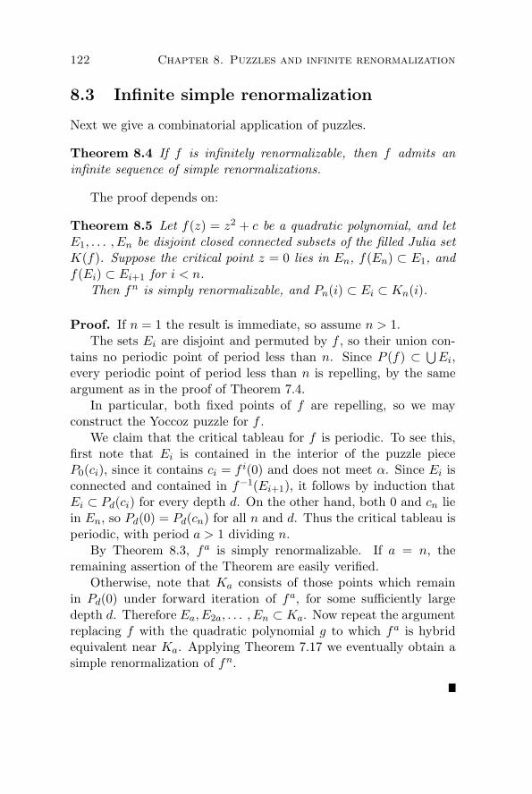
122 Chapter 8. Puzzles and infinite renormalization
8.3 Infinite simple renormalization
Next we give a combinatorial application of puzzles.
Theorem 8.4 If f is infinitely renormalizable, then f admits aninfinite sequence of simple renormalizations.
The proof depends on:
Theorem 8.5 Let f(z) = z2 + c be a quadratic polynomial, and letE1, . . . , En be disjoint closed connected subsets of the filled Julia setK(f). Suppose the critical point z = 0 lies in En, f(En) ⊂ E1, andf(Ei) ⊂ Ei+1 for i < n.
Then fn is simply renormalizable, and Pn(i) ⊂ Ei ⊂ Kn(i).
Proof. If n = 1 the result is immediate, so assume n > 1.The sets Ei are disjoint and permuted by f , so their union con-
tains no periodic point of period less than n. Since P (f) ⊂⋃Ei,
every periodic point of period less than n is repelling, by the sameargument as in the proof of Theorem 7.4.
In particular, both fixed points of f are repelling, so we mayconstruct the Yoccoz puzzle for f .
We claim that the critical tableau for f is periodic. To see this,first note that Ei is contained in the interior of the puzzle pieceP0(ci), since it contains ci = f i(0) and does not meet α. Since Ei isconnected and contained in f−1(Ei+1), it follows by induction thatEi ⊂ Pd(ci) for every depth d. On the other hand, both 0 and cn liein En, so Pd(0) = Pd(cn) for all n and d. Thus the critical tableau isperiodic, with period a > 1 dividing n.
By Theorem 8.3, fa is simply renormalizable. If a = n, theremaining assertion of the Theorem are easily verified.
Otherwise, note that Ka consists of those points which remainin Pd(0) under forward iteration of fa, for some sufficiently largedepth d. Therefore Ea, E2a, . . . , En ⊂ Ka. Now repeat the argumentreplacing f with the quadratic polynomial g to which fa is hybridequivalent near Ka. Applying Theorem 7.17 we eventually obtain asimple renormalization of fn.

8.4. Measure and local connectivity 123
Proof of Theorem 8.4. For each level of renormalization n inR(f),let κn denote the number of components of Kn and let µn denote themultiplicity of the renormalization (the maximal number of filledJulia sets meeting at a single point — see §7.3.) Then n = κnµn.
We claim κn tends to infinity. Indeed, let x be a point where twoor more small filled Julia sets at level n meet; then x is a repellingperiodic point of f , and κn is at least as large as the period of x. ByTheorem 7.8 (High periods), the period of x tends to infinity as ntends to infinity.
Next we show fa is simply renormalizable for a = κn. To thisend, let E1, . . . , Ea denote the components of Kn, ordered so that thecritical point 0 lies in Ea and f(Ei) = Ei+1. Then the hypotheses ofTheorem 8.5 are satisfied, so fa is simply renormalizable. Since κn →∞, the map f admits an infinite sequence of simple renormalizations.
8.4 Measure and local connectivity
In this section we summarize results of Lyubich, Shishikura and Yoc-coz which are proved using the Yoccoz puzzle.
Theorem 8.6 (Yoccoz) Let f(z) = z2+c be a quadratic polynomialsuch that
1. the Julia set J(f) is connected,
2. f has no indifferent cycle, and
3. f is not infinitely renormalizable.
Then J(f) is locally connected.If, in addition, f has no attracting cycle, then c lies in the bound-
ary of the Mandelbrot set M and M is locally connected at c.
See [Yoc]; a detailed proof of local connectivity of J(f) underslightly stronger assumptions can be found in [Mil3].

124 Chapter 8. Puzzles and infinite renormalization
Corollary 8.7 If the Julia set of f(z) = z2 + c carries an invariantline field, then fn is simply renormalizable for infinitely many n.
Proof. By Theorems 4.8 and 4.9, if f admits an invariant linefield, then c lies in a non-hyperbolic component of the interior ofthe Mandelbrot set and every periodic cycle of f is repelling. So byYoccoz’s result, f is infinitely renormalizable, and by Theorem 8.4infinitely many of these renormalizations are simple.
An alternative route to the Corollary above is given by the fol-lowing result:
Theorem 8.8 (Lyubich, Shishikura) If f(z) = z2 + c has no in-different cycles and J(f) has positive measure, then f is infinitelyrenormalizable.
See [Lyu4].Here is the skeleton of Lyubich’s argument. Applying the Yoccoz
puzzle, a new type of polynomial-like mapping, and a version ofTheorem 2.16, Lyubich first proves:
Theorem 8.9 Let f be a quadratic polynomial with both fixed pointsrepelling. Then either the Julia set of f has measure zero, or fn isrenormalizable for some n > 1.
Now suppose f has no indifferent cycles and J(f) has positivemeasure. By the result above, fa is renormalizable for some a > 1.To establish the theorem, one need only show that for any such athere is a c > a such that f c is also simply renormalizable.
By Theorem 5.7, there is a quadratic polynomial g to which fa
is hybrid equivalent. By a generalization of Theorem 8.2, almost ev-ery point in J(f) eventually lands in Ja, so Ja has positive measure.Quasiconformal maps in the plane preserve sets of positive measure[LV, §IV.1.4], so J(g) has positive measure. Since f has no indifferentcycle, both fixed points of g are repelling, and thus gb is renormal-izable for some b > 1. By Theorem 7.17, f c is renormalizable forc = ab.

8.5. Laminations and tableaux 125
Remark. Actually, in the arguments of both Yoccoz and Lyubich,periodicity of the critical tableau is used to construct renormaliza-tions. So these renormalizations are always simple by Theorem 8.3.
8.5 Laminations and tableaux
In this section we show the tableau of a quadratic polynomial isdetermined by the external angles of the inverse images of the α fixedpoint. It follows that renormalizability can be checked by looking atexternal rays; this fact will be used in Appendix B.
Recall from §6.4 that a lamination is an equivalence relation onthe circle such that the convex hulls of distinct equivalence classesare disjoint. As in that section, we will identify the circle S1 = R/Zwith the boundary of the disk via the map t +→ exp(2πit).
Let f(z) = z2+c be a quadratic polynomial with connected Juliaset, whose fixed points are labeled α and β as in §6.2.
Definition. The α-lamination λα(f) ⊂ λQ(f) is the subset of therational lamination corresponding to rays which land in the inverseorbit of α. That is, (t, t′) ∈ λα(f) if and only if t = t′ or t and t′ areboth rational, the external rays Rt and Rt′ land at the same pointz ∈ J(f), and fn(z) = α for some n ≥ 0.
Now suppose both fixed points α and β of f are repelling, andthe forward orbit of the critical point of f is disjoint from α. Thenthe critical tableau Pn(ck) for the Yoccoz puzzle is well-defined.
We will show that the critical tableau can be reconstructed fromthe α-lamination of f . To make this precise, we will construct amodel tableau Gn,k canonically from λα(f).
Let F : S1 → S1 be defined by F (t) = 2t. Since every point inthe inverse image of α is prefixed, there is a natural stratification
λα(f) =∞⋃
0
λdα(f), λ0α(f) ⊂ λ1α(f) ⊂ λ2α(f) ⊂ . . . ,
given by
λ0α(f) = λα(f) ∩ (t, t′) : t = t′ or t and t′ are periodic under F,
andλdα(f) = λα(f) ∩ (t, t′) : (F d(t), F d(t′)) ∈ λ0α(f)

126 Chapter 8. Puzzles and infinite renormalization
for d > 0. The lamination λ0α(f) has a unique nontrivial equivalenceclass, corresponding to the finite set of rays landing at α. Similarlyλdα(f) corresponds to the rays landing in f−d(α).
For each lamination λdα(f), let Λd ⊂ ∆ be the union of the convexhulls of equivalence classes in λdα(f). A gap at depth d is the closureof a component of ∆− Λd. Let Gd be the set of such gaps.
For any gap G at depth d+ 1, there is a unique map G′ at leveld such that F (G ∩ S1) = G′ ∩ S1; we denote this new gap by F (G).
A gap G at depth d > 0 is critical if F is 2-to-1 on the interior ofG ∩ S1. By definition, the unique largest gap at depth d = 0 is alsocritical.
Now let Pd denote the pieces at depth d in the Yoccoz puzzle for f .Since Λd separates the disk in the same pattern as the rays landingat f−d(α) separate the plane, there is a natural depth-preservingbijection
φ : ⨿Pd → ⨿Gd
between the disjoint unions of the pieces and the gaps, such that:
1. an external ray Rt enters P ∈ Pd if and only if exp(2πit) ∈φ(P ) ∈ Gd;
2. the critical point z = 0 belongs to P if and only if φ(P ) is acritical gap; and
3. if P is a puzzle piece at depth d > 0, then φ(f(P )) = F (φ(P )).
The model tableau is constructed by setting Gd,0 equal to the
unique critical gap at depth d, and defining Gd,k = F k(Gd+k,0). Themodel tableau is canonically determined by λα(f).
It is immediate that
φ(Pd(ck)) = φ(Pd(fk(0))) = φ(fk(Pd+k(0))) = F k(Gd+k,0)
= Gd,k,
so we have established:
Theorem 8.10 There is a natural bijection φ between puzzle piecesand gaps which sends the critical piece Pd(ck) to the gap Gd,k.

8.5. Laminations and tableaux 127
Figure 8.2. The α-lamination for z2 + i, to depth four.
pics/Puz.1.6.ps not found
Figure 8.3. The puzzle pieces for z2 + i, to depth four.

128 Chapter 8. Puzzles and infinite renormalization
Example. Let f(z) = z2 + i. The hyperbolic convex hulls of theequivalence classes of λ4α(f) are depicted in Figure 8.2; the puzzlepieces of depth four or less for the same map are shown in Figure8.3.
Definition. The model tableau is periodic if for some n > 0, Gd,0 =Gd,n for all depths d. The least such n is the period of the modeltableau.
By Theorem 8.3 we have:
Corollary 8.11 The period of the model tableau Gd,k is equal to therenormalization period of f .
Theorem 8.12 Let f and g be quadratic polynomials, each with con-nected Julia set, both fixed points repelling, and the forward orbit ofthe critical point disjoint from the α fixed point.
Suppose λα(f) ⊂ λα(g). Then λα(f) = λα(g) and the renormal-ization period of f is equal to that of g.
Proof. Suppose λα(f) ⊂ λα(g). By Theorem 7.9, the external rayslanding at the α fixed point are permuted transitively. In particular,the external angle of one ray landing at α determines the entire set ofrays landing at α. Since λ0α(f) ⊂ λ0α(g), and the former equivalencerelation is nontrivial, we have λ0α(f) = λ0α(g). Since the forwardorbit of the critical point avoids α, the cardinalities of f−d(α) andg−d(α) are the same (2d+1 − 1), and so λdα(f) and λdα(g) have thesame number of nontrivial equivalence classes. Thus λdα(f) ⊂ λdα(g)implies λdα(f) = λdα(g) and therefore λα(f) = λα(g).
Since λα determines the model tableau, the preceding result showsf and g have the same renormalization period.
Remarks. This theorem fails if we do not require both fixed to berepelling. For example, if we set f(z) = z2 − 1 and g(z) = z2 − 3/4,then f2(z) is renormalizable and λα(f) = λα(g), but g2(z) is notrenormalizable because its α fixed point is parabolic.
Also, if we allow the critical point to land on α, then λα(f) ⊂λα(g) does not imply λα(f) = λα(g). An example is provided bytaking f(z) = z2 − 1 and g(z) = z2 − 1.54368..., where g3(0) is theα-fixed point of g. (Here g is the same as Example III of §7.4.)

Chapter 9
Robustness
In this chapter we turn to the geometric aspects of infinitely renor-malizable polynomials. First, we define a canonical set of disjointsimple geodesics on the Riemann surface C−P (f). The disks boundedby these geodesics are like the basic intervals in the construction ofa Cantor set. When these geodesics have length bounded above atinfinitely many levels, we say the polynomial is robust. We showthat the postcritical set of a robust polynomial is a Cantor set ofzero area, and give a topological model for its dynamics.
9.1 Simple loops around the postcritical set
Definitions. Let f be infinitely renormalizable. Then |SR(f)| = ∞by Theorem 8.4. Let SR(f)∗ = SR(f)− 1.
For each level n in SR(f)∗, let γn(i) denote the hyperbolic geodesicon C−P (f) representing a simple closed curve separating Jn(i) fromP (f)− Jn(i). This curve exists because Pn(j) is disjoint from Jn(i)for any i = j (Theorem 8.1), its homotopy class is unique becauseJn(i) is connected, and it is represented by a geodesic because n > 1.
Let γn = γn(n) denote the loop encircling the critical point of f .
The terminology “simple renormalization” is motivated by thefollowing:
129

130 Chapter 9. Robustness
Theorem 9.1 (Simple curves) The geodesics
Γ = γn(i) : n ∈ SR(f)∗ and 1 ≤ i ≤ n
are simple and disjoint.
Proof. A hyperbolic geodesic is simple if there is a simple represen-tative in its homotopy class, and two distinct geodesics are disjointif they are homotopic to disjoint curves. Thus γn(i) is simple bydefinition.
Now consider two geodesics γa(i) and γb(j). We can find repre-sentatives of these curves in C − P (f) which are arbitrarily close toJa(i) and Jb(j). If these small Julia sets are disjoint, then so areγa(i) and γb(j).
Otherwise Ja(i) meets Jb(j). If a = b, then Ja(i)∩Jb(j) is a singlepoint x, a periodic point of f which does not belong to the postcriticalset. Since the renormalization is simple, x does not disconnect Ja(i)or Ja(j). Thus we can represent γa(i) and γb(j) by homotopic curveswhich are disjoint, so the geodesic representatives are also disjoint.
Finally suppose a < b. Then Jb(j) ⊂ Ja(k) for some k. It isobvious that γb(j) can be represented by a curve nested inside γa(k)in this case. Since the geodesics at level a bound disjoint disks, weneed only rule out the possibility that k = i and γa(i) = γb(j). Butthere is a portion P ′ of the postcritical set lying in Ja(i) − Jb(j), soγa(i) and γb(j) lie in different homotopy classes on C − P (f), andthus they are distinct and disjoint.
Theorem 9.2 (Invariant curve system) Let n belong to SR(f)∗.For i = 1, f−1(γn(i)) has a component α which is isotopic to
γn(i − 1) on C − P (f) and covers γn(i) by degree one. The othercomponent β bounds a disk disjoint from the postcritical set.
For i = 1, f−1(γn(1)) = α is a connected curve isotopic to γn(n)and covering γn(1) by degree two.
Proof. The curve γn(i) is isotopic on C−P (f) to a loop separatingJn(i) from P (f) − Jn(i). For i = 1 the critical value does not lie

9.1. Simple loops around the postcritical set 131
in Jn(i), so the preimage of this loop has two components. One ofthem, α, separates Jn(i− 1) from P (f)− Jn(i− 1), and therefore isisotopic to γn(i− 1). The other component β is isotopic to a loop ina small neighborhood of J ′
n(i− 1). Since J ′n(i− 1) does not meet the
postcritical set, β bounds a disk on C− P (f).When i = 1, the critical value lies in Jn(1), so f−1(γn(1)) = α
covers γn(1) by degree two and α is isotopic to a curve enclosingJn(n).
Remark. As a consequence, the set of homotopy classes
Γn = γn(1), . . . , γn(n)
on C− P (f) is an f -invariant curve system; see §B.2.Let ℓ(·) denote length in the hyperbolic metric on C− P (f).
Theorem 9.3 (Comparable lengths) For any n in SR(f)∗, thehyperbolic lengths of the geodesics γn(i) at a given level n are com-parable; in fact
1
2ℓ(γn(n)) ≤ ℓ(γn(1)) ≤ . . . ≤ ℓ(γn(n− 1)) ≤ ℓ(γn(n)).
Proof. Let Q = f−1(P (f)). For 1 < i ≤ n, the preimage f−1(γn(i))has a component α isotopic to γn(i−1) and covering γn(i) by degreeone. Since f : (C−Q) → (C−P ) is a covering, it is an isometry for therespective Poincare metrics, while the inclusion (C−Q) → (C− P )is a contraction, so
ℓ(γn(i− 1)) ≤ ℓ(α) ≤ ℓ(γn(i)).
Finally f−1(γn(1)) = α is isotopic to γn(n) and covers γn(1) bydegree two, which implies ℓ(γn(n)) ≤ 2ℓ(γn(1)).

132 Chapter 9. Robustness
9.2 Area of the postcritical set
Definition. A quadratic polynomial f(z) = z2 + c is robust if f isinfinitely renormalizable, and
lim infSR(f)∗
ℓ(γn) < ∞,
where ℓ(·) denotes hyperbolic length on C− P (f).Note that robustness is a property of the geometry of the postcrit-
ical set. The small Julia sets enter only in a combinatorial fashion,to pick out the simple closed curves γn.
The main result of this section is:
Theorem 9.4 (Postcritical measure zero) Let f be robust. Then:
1. The postcritical set P (f) is a Cantor set of measure zero.
2. As n → ∞ in SR(f),
supi
diamPn(i) → 0.
3. f : P (f) → P (f) is a homeomorphism, which is topologicallyconjugate to the map x +→ x+ 1 acting on the group
proj limn∈SR(f)
Z/n.
The proof is based on the Collar Theorem and the area zerocriterion of §2.8. So we actually obtain the stronger result that P (f)has absolute area zero.
Proof. Let SR(f)∗ = n(1), n(2), n(3), . . . with n(k) < n(k + 1).For each k, and for i = 1, . . . , n(k), let Ak(i) be the standard
collar C(γn(k)(i)) about the geodesic γn(k)(i) on the hyperbolic sur-
face C − P (f), as defined in §2.9. By the Collar Theorem 2.18, thecollection of annuli obtained in this way are disjoint. Note that Ak(i)separates Pn(k)(i) from the rest of the postcritical set.

9.2. Area of the postcritical set 133
Let Ek be the union of the annuli around the small postcriticalsets at level n(k); that is,
Ek =n(k)⋃
i=1
Ak(i).
By Corollary 7.16, any small postcritical set Pn(k+1)(i) is contained inPn(k)(j) for some j; therefore any annulus Ak+1(i) in Ek+1 is nestedinside some annulus Ak(j) in Ek.
We are assuming lim inf ℓ(γn) < ∞. By Theorem 9.3, the geodesicsat a given level n(k) have length bounded above by ℓ(γn(k)). There-fore the sum of the moduli of all annuli nested around an arbitrarypoint x ∈ P (f) diverges, by Theorem 2.19. Applying Theorem 2.16,we conclude that the nested intersection F =
⋂Fk is a totally dis-
connected set of measure zero, where Fk is the union of the boundedcomponents of C − Ek. But each component of Fk meets P (f), soF = P (f) and we have shown that the postcritical set has measurezero.
Note that Fk is a decreasing sequence of compact sets and Pn(k)(i)lies in a single component of Fk for any i. Since F is totally discon-nected, the diameter of the largest component of Fk tends to zero,so supi diam(Pn(k)(i)) tends to zero as well.
For each n ∈ SR(f), there is a natural map P (f) → Z/n sendingPn(i) to imodn. These maps are compatible as n varies, so theydetermine a continuous map
φ : P (f) → proj limn∈SR(f)
Z/n.
We have just seen that the small postcritical sets nest down to points,so this map is injective; and it conjugates f to x +→ x + 1 becausef(Pn(i)) = Pn(i+1). The projectively limit is a Cantor set, so P (f)is also a Cantor set.
Remarks. The theorem also holds under the weaker hypothesis∑
SR(f)∗modC(γn) = ∞,

134 Chapter 9. Robustness
where C(·) denotes the collar about γn.It seems unlikely that every infinitely renormalizable quadratic
polynomial is robust. A natural test case is provided by an example ofDouady and Hubbard, where f(z) = z2+c is infinitely renormalizablebut the Julia set J(f) is not locally connected [Mil3, §3].
We do not know if robustness implies the Julia set is locally con-nected, or has measure zero. Robustness seems to give more controlover the postcritical set than the Julia set. Of course it would alsobe interesting to know if the Mandelbrot set is locally connected atc when z2 + c is robust.

Chapter 10
Limits of renormalization
This chapter is devoted to the proof of our main result, which werestate:
Theorem 1.7 (Robust rigidity) A robust infinitely renormalizablequadratic polynomial f carries no invariant line field on its Julia set.
This theorem is equivalent to the statement that any quadraticpolynomial g which is quasiconformally conjugate to f is conformallyconjugate to f . Because the theorem rules out quasiconformal de-formations, we call it a rigidity result.
Recall that an infinitely renormalizable quadratic polynomial fis robust if
lim infSR(f)∗
ℓ(γn) = L < ∞.
We will divide the proof into two cases, depending on whether or notL = 0.
Both arguments follow the same pattern, which we now brieflysummarize. Suppose f is infinitely renormalizable, robust, and car-ries an invariant line field µ on its Julia set. To deduce a contradic-tion, we pass to a subsequence of n in SR(f) such that after rescaling,fn converges on a neighborhood of the small postcritical Pn. Thelimiting dynamical system f∞ will be a proper map of degree two.Robustness furnishes the compactness required in this step.
Next we use µ to construct a univalent invariant line field for f∞.Pick a point x in the Julia set of f where µ is almost continuous,
135

136 Chapter 10. Limits of renormalization
such that ∥(fk)′x∥ → ∞ with respect to the hyperbolic metric onC−P (f) as k → ∞, and such that fk(x) tends to (but does not landin) P (f) as k → ∞. We would like to push µ forward univalentlyfrom a small neighborhood of x to a definite neighborhood of Pn.
The idea for obtaining a univalent pushforward is summed up inFigure 10.1. The circles labeled 1, 2, . . . , n denote neighborhoods ofthe small postcritical sets Pn(1), Pn(2), . . . , Pn(n). (The exact choiceof neighborhood of Pn(i) varies between the cases L = 0 and L > 0;in the simpler case where L = 0, Vn(i) will do.) For i = 1, . . . , n− 1,region i maps to region i + 1 univalently. Region n contains thecritical point and maps over Pn(1) by degree two (it may or maynot map over region 1). Each region other than 1 has a primedcompanion with the same image.
x
2
3
n 1
1′
2′
i′ i
i+ 1
Figure 10.1. Pattern of the proof: univalent pushforward from x.
Since x is attracted to the postcritical set, it eventually entersthe cycle of regions at level n. Just before it does so, it must enter aprimed region i′. This region is disjoint from the postcritical set, so itadmits a univalent pushforward from a neighborhood of x. There issufficient expansion in the hyperbolic metric on C−P (f) to guaranteethat this pushforward of µ is nearly univalent. The map fn−i carriesthis line field around to a neighborhood of Pn. In the limit we obtain

10.1. Unbranched renormalization 137
a univalent invariant line field for f∞. But this is impossible, becausef∞ has a critical point. Thus the original dynamical system f hasno invariant line field either.
When L = 0 (or indeed when L is sufficiently small), the limit-ing dynamical system f∞ can be chosen to be a quadratic-like map(rather than just a proper map). This is the simplest situation toanalyze, and it is treated in §10.1 and §10.2.
When L > 0, we can still construct a limiting proper map ofdegree two, but it may not be quadratic-like. In the course of theconstruction, we also cannot assume that the preimage of region 1is contained in region n. Thus there is an additional possibility toanalyze, when x lands in between. The new features which arise inthis case are dealt with in §10.3 and §10.4.
10.1 Unbranched renormalization
Let f be a quadratic polynomial which admits an infinite sequenceof simple renormalizations.
Definition. A renormalization fn : Un → Vn is unbranched if
Vn ∩ P (f) = Pn.
Theorem 10.1 If fn : Un → Vn is an unbranched renormalization,then V ′
n(i) is disjoint from the postcritical set of f for i = n.
Proof. The small postcritical sets are disjoint and f(Pn(i)) ⊂ Pn(i+1), so when fn : Un → Vn is unbranched we have Vn(i) ∩ P (f) =Pn(i). Since Vn(i) and V ′
n(i) have the same image under f , any pointin V ′
n(i) ∩ P (f) must lie in Pn(i). But Vn(i) and V ′n(i) are disjoint
for i = n.
Therefore f−k can be defined univalently on V ′n(i) for any k > 0.
The existence of univalent inverses is the reason for the terminology“unbranched”.
In the next section, we will establish:

138 Chapter 10. Limits of renormalization
Theorem 10.2 (Polynomial-like rigidity) Let f be a quadraticpolynomial and let m > 0 be a constant. Suppose for infinitely manyn > 1 there is a simple unbranched renormalization fn : Un → Vn
with mod(Un, Vn) > m > 0.Then the Julia set of f carries no invariant line field.
Assuming this theorem for the moment, we can deduce the mainrigidity result in the case where lim inf ℓ(γn) is sufficiently small. Todo this, we must relate the length of γn to the existence of unbranchedrenormalizations.
Theorem 10.3 Suppose f is infinitely renormalizable and fn is sim-ply renormalizable. Then we may choose Un and Vn such that therenormalization fn : Un → Vn is unbranched. When ℓ(γn) is suffi-ciently small, we can also ensure
mod(Un, Vn) > m(ℓ(γn)) > 0,
where m(ℓ) → ∞ as ℓ→ 0.
Proof. We can always choose Vn very close to Jn, by starting withan arbitrary renormalization and replacing Vn with a component off−nd(Vn) for large d. Since P (f)−Kn is closed, this renormalizationis unbranched when Vn is sufficiently close to Kn.
To complete the proof, we will show that when γn is a shortgeodesic on C − P (f), there is an unbranched renormalization withmod(Un, Vn) large.
Let An be the collar C(γn) about γn with respect to the hyper-bolic metric on C − P (f). The modulus of An is large when ℓ(γn)is small (cf. Theorems 2.18 and 2.19.) Let Bn be the componentof f−n(An) which lies in the same homotopy class as γn. Constructopen disks Dn and En by adjoining to An and Bn the bounded com-ponents of their complements; then fn : Dn → En is a proper mapof degree two, and
Dn ∩ P (f) = En ∩ P (f) = Pn
so fn : Dn → En is a critically compact proper map (in the sense of§5.5.)

10.1. Unbranched renormalization 139
Since f is infinitely renormalizable, it has no attracting cycles.By Theorem 5.12, we can find a renormalization fn : Un → Vn
with Un ⊂ Dn and Vn ⊂ En whenever mod(Pn, En) is sufficientlylarge. Moreover, the renormalization can be constructed so thatmod(Un, Vn) is bounded below in terms of mod(Pn, En). Clearly
mod(Pn, En) ≥ mod(An) = mod(C(γn)),
and the modulus of the collar depends only on ℓ(γn) and tends toinfinity as ℓ(γn) tends to zero. Thus mod(Un, Vn) is bounded belowin terms of ℓ(γn), and the theorem follows.
Corollary 10.4 (Thin rigidity) There is a constant L > 0 suchthat if
lim infSR(f)∗
ℓ(γn) < L,
then f carries no invariant line field on its Julia set.
In particular, the theorem holds if lim inf ℓ(γn) = 0. This condi-tion implies the Riemann surface C− P (f) has infinitely many verythin parts.
Proof. By the previous theorem, there exists an L > 0 such thatfn admits an unbranched renormalization with mod(Un, Vn) > 1whenever ℓ(γn) < L. So the corollary follows by Theorem 10.2.
The following corollary is not used in the sequel, but it clari-fies the picture of thin rigidity. It also shows that many infinitelyrenormalizable maps — such as the Feigenbaum polynomial — donot satisfy lim infSR(f)∗ ℓ(γn) = 0. In §10.3 we will prove rigidity forrobust polynomials with lim infSR(f)∗ ℓ(γn) > 0.
Corollary 10.5 There is a constant L′ > 0 such that for any in-finitely renormalizable quadratic polynomial f , and any n ∈ SR(f)∗,ℓ(γn) < L′ implies the renormalization of fn is of disjoint type (thesmall Julia sets at level n do not touch).

140 Chapter 10. Limits of renormalization
Proof. Suppose ℓ(γn) is small. Then the collar lemma provides alarge annulus separating Pn(i) from P (f) − Pn(i) for each i. Thisannulus contains a round annulus of comparable modulus (Theorem2.1), so
diamPn(i) ≪ d(Pn(i), P (f) − Pn(i))
in the Euclidean metric. By Theorem 10.3, the polynomial-like map-pings fn : Un(i) → Vn(i) can be chosen with mod(Un, Vn) large aswell. Since fn is infinitely renormalizable, it has no attracting cycles,so by Corollary 5.10
diam(Kn(i)) = O(diam(Pn(i))).
Combining these two estimates, we conclude the sets Kn(i) are dis-joint when ℓ(γn) is sufficiently small. In fact
d(Kn(i),Kn(j))
diamKn(i)≥ C(ℓ(γn))
where C(ℓ) → ∞ as ℓ→ 0.
10.2 Polynomial-like limits of renormalization
In this section we prove Theorem 10.2 (Polynomial-like rigidity).First we obtain some preliminary information about unbranchedrenormalizations with definite moduli. This will enable us to con-struct a suitable point x from which to push the line field forward.Then we will pass to a limit (using compactness of quadratic-likemaps with mod(U, V ) > m) and obtain a contradiction.
Theorem 10.6 Suppose the renormalization of fn is unbranchedand mod(Un, Vn) > m > 0. Then for i = n, the companion Juliaset satisfies
diam(J ′n(i)) ≤ C(m)
in the hyperbolic metric on C− P (f).
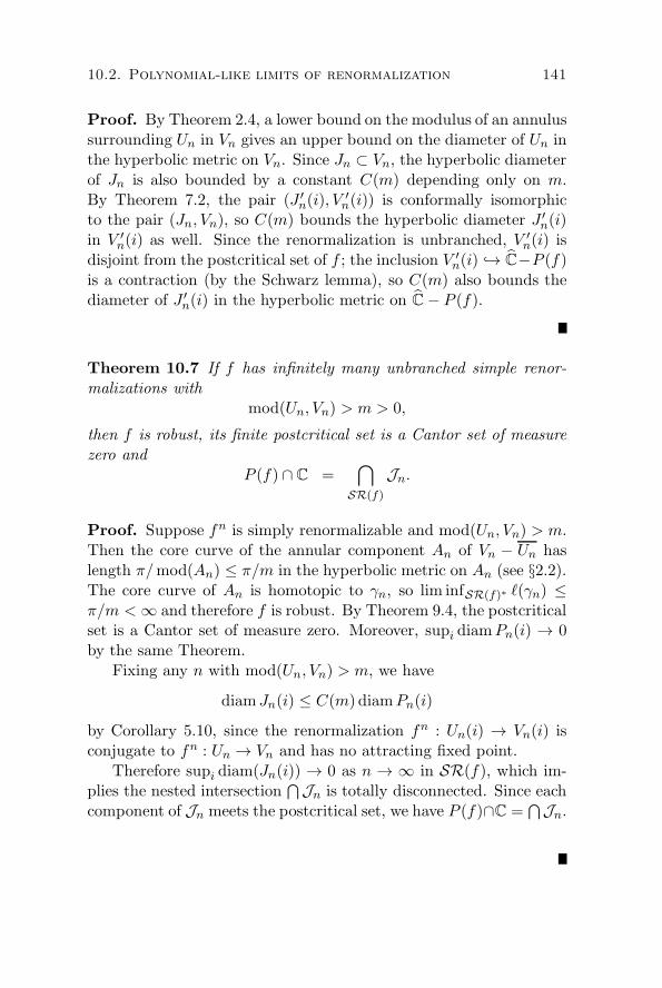
10.2. Polynomial-like limits of renormalization 141
Proof. By Theorem 2.4, a lower bound on the modulus of an annulussurrounding Un in Vn gives an upper bound on the diameter of Un inthe hyperbolic metric on Vn. Since Jn ⊂ Vn, the hyperbolic diameterof Jn is also bounded by a constant C(m) depending only on m.By Theorem 7.2, the pair (J ′
n(i), V′n(i)) is conformally isomorphic
to the pair (Jn, Vn), so C(m) bounds the hyperbolic diameter J ′n(i)
in V ′n(i) as well. Since the renormalization is unbranched, V ′
n(i) isdisjoint from the postcritical set of f ; the inclusion V ′
n(i) → C−P (f)is a contraction (by the Schwarz lemma), so C(m) also bounds thediameter of J ′
n(i) in the hyperbolic metric on C− P (f).
Theorem 10.7 If f has infinitely many unbranched simple renor-malizations with
mod(Un, Vn) > m > 0,
then f is robust, its finite postcritical set is a Cantor set of measurezero and
P (f) ∩ C =⋂
SR(f)
Jn.
Proof. Suppose fn is simply renormalizable and mod(Un, Vn) > m.Then the core curve of the annular component An of Vn − Un haslength π/mod(An) ≤ π/m in the hyperbolic metric on An (see §2.2).The core curve of An is homotopic to γn, so lim infSR(f)∗ ℓ(γn) ≤π/m < ∞ and therefore f is robust. By Theorem 9.4, the postcriticalset is a Cantor set of measure zero. Moreover, supi diamPn(i) → 0by the same Theorem.
Fixing any n with mod(Un, Vn) > m, we have
diam Jn(i) ≤ C(m) diamPn(i)
by Corollary 5.10, since the renormalization fn : Un(i) → Vn(i) isconjugate to fn : Un → Vn and has no attracting fixed point.
Therefore supi diam(Jn(i)) → 0 as n → ∞ in SR(f), which im-plies the nested intersection
⋂Jn is totally disconnected. Since each
component of Jn meets the postcritical set, we have P (f)∩C =⋂Jn.

142 Chapter 10. Limits of renormalization
Corollary 10.8 Under the same hypotheses, almost every point xin J(f) has the following properties:
1. the forward orbit of x does not meet the postcritical set;
2. ∥(fn)′(x)∥ → ∞ in the Poincare metric on C− P (f);
3. for any n ∈ SR(f), there is a k > 0 such that fk(x) ∈ Jn; and
4. for any k > 0, there is an n ∈ SR(f) such that fk(x) does notmeet Jn.
Proof. By the preceding Theorem, P (f) has measure zero; therefore⋃f−n(P (f)) has measure zero, establishing point one. The second
and third points follow by Theorems 3.6 and 8.2.To verify the last property, note that by the preceding The-
orem, area(Jn) = 0 as n → ∞ in SR(f). Fixing k, we havearea(f−k(Jn)) → 0 as well, and therefore
⋂n f
−k(Jn) has measurezero.
Proof of Theorem 10.2 (Polynomial-like rigidity). LetUSR(f,m) be an infinite set of n such that fn : Un → Vn is anunbranched simple renormalization and mod(Un, Vn) > m.
Suppose f admits an invariant line field µ supported on a set Eof positive measure in the Julia set. Let x ∈ E be a point of almostcontinuity of µ which also satisfies the properties guaranteed by theCorollary above. For each n ∈ SR(f), let k(n) ≥ 0 be the leastnon-negative integer such that fk(n)+1(x) ∈ Jn. By our choice of x,k(n) → ∞.
Consider n ∈ USR(f,m) sufficiently large that k(n) > 0. Thenfk(n)+1(x) ∈ Jn but fk(n)(x) is not in Jn. Therefore fk(n)(x) liesin some companion Julia set J ′
n(i(n)) where 0 < i(n) < n. (Notefk(n)+1(x) cannot lie in Jn(1) since that would imply fk(n)(x) ∈Jn(n) ⊂ Jn.)
Since the nth renormalization is unbranched, there is a univalentbranch of f−k(n) defined on V ′
n(i(n)) and carrying fk(n)(x) back to

10.2. Polynomial-like limits of renormalization 143
fn
fk(n)
Vn(i(n))
hn
VnV ′n(i(n))
x
fn−i(n)
J ′n(i(n))
Un
Jn(i(n))
fn−i(n)
Figure 10.2. Expanding a line field into a polynomial-like map.
x. The map fn−i(n) : V ′n(i(n)) → Vn is also univalent. Define a
univalent map hn : Vn → C by the composition
Vnf i(n)−n
−−−−→ V ′n(i(n))
f−k(n)
−−−−→ C
using the branches of the inverse mentioned above. See Figure 10.2.By invariance, µ|Vn = h∗n(µ).
LetJ∗n = hn(Jn) = f−k(n)(J ′
n(i(n)))
be the small copy of the Julia set containing x. Since the diameterof J ′
n(i(n)) in the hyperbolic metric on C − P (f) is bounded above(Theorem 10.6), and ∥(fk(n))′(x)∥ → ∞, we have
diam(J∗n) → 0
in the hyperbolic metric on C − P (f). (To show the derivative atone point controls the size of J∗
n, we may appeal to Theorem 3.8 orto the Koebe distortion theorem.)

144 Chapter 10. Limits of renormalization
Thus the line field µ = h∗n(µ) is invariant under fn and close toa univalent line field on Vn.
Let An(z) = z/diam(Jn), let gn = An fn A−1n , and let yn =
An(h−1n (x)). Then
gn : (An(Un), 0) → (An(Vn), An(fn(0)))
is a quadratic-like map with diam(J(gn)) = 1, satisfying
mod(An(Un), An(Vn)) ≥ m.
Since h−1n (x) ∈ Jn, we have yn ∈ J(gn).
By Theorem 5.8, there is a subsequence of n in USR(f,m) suchthat gn converges in the Caratheodory topology to a quadratic-likemap
g : (U, 0) → (V, g(0))
with mod(U, V ) ≥ m.Let kn = hn A−1
n denote the composition
An(Vn)A−1
n−−→ Vnhn−→ C.
Then kn(yn) = x and νn = k∗n(µ) is a gn-invariant line field onAn(Vn).
Since 1 = diam(J(gn)), while diam(kn(J(gn))) = diam(J∗n) → 0,
we have k′n(yn) → 0 by the Koebe theorem. The fact that yn ∈ J(gn)and the Julia set is surrounded by an annulus of definite modulusin An(Vn) implies for a further subsequence, (An(Vn), yn) → (V, y)by Theorem 5.3. By Theorem 5.16, after passing to a further subse-quence, νn converges to a univalent g-invariant line field ν on V .
As the renormalizations fn have connected Julia sets, so does g;therefore the critical point and critical value of g lie in V . But theng admits no univalent invariant line field (by Theorem 5.13).
Therefore f itself has no measurable invariant line field.
Remark. When lim infSR(f)∗ ℓ(γn) = 0, the proof above takes a par-ticularly simple form. In this case, the polynomial-like maps gn canbe chosen to converge to a quadratic polynomial g : C → C, and theline fields νn to the family ν of horizontal lines in the plane. Clearlyν fails to be g-invariant; indeed the only polynomials preserving νare the linear maps az + b with a ∈ R.

10.3. Proper limits of renormalization 145
10.3 Proper limits of renormalization
In this section and the next we complete the proof of Theorem 1.7(Robust rigidity) by establishing:
Theorem 10.9 (Thick rigidity) Let f(z) = z2 + c be infinitelyrenormalizable, and suppose
0 < lim infSR(f)∗
ℓ(γn) < ∞.
Then f carries no invariant line field on its Julia set.
The proof follows the same outline as the proof in §10.2. There isone important difference: we do not use polynomial-like mappings.Indeed, we do not know if a robust quadratic polynomial admits in-finitely many renormalizations with mod(Un, Vn) > m > 0.1 Becauseof this we have no control over the shape of the small Julia sets.
This makes it more difficult to say when the forward orbit ⟨fk(x)⟩first enters the influence of a given level n of renormalization (whereasbefore we could simply look at the least k such that fk(x) ∈ Jn). Totake care of this, we will show that by the time fk(x) is quite closeto a small postcritical set Pn(i) at level n, it has already passed closeto some companion postcritical set P ′
n(j) at the same level. In thisway we will obtain a nearly univalent invariant line field near P ′
n(j),and from that a contradiction.
To carry out the proof, we will need infinitely many geodesicsγn which are neither too long nor too short, to obtain a kind ofbounded geometry. Thus the arguments in the thick and thin cases,while similar, are really distinct: neither one contains the other.
Definitions. We collect together some additional notation. Foreach n ∈ SR(f)∗:
• δn denotes the unique component of f−n(γn) which is isotopicto γn on C− P (f). This curve exists by Theorem 9.2.
• Xn denotes the disk in C bounded by δn.
1Sullivan has obtained a proof of this property for real quadratics of boundedtype; see [Sul4].

146 Chapter 10. Limits of renormalization
Pn
Yn
fn
Xn
Figure 10.3. Proper map of degree two at level n.
• Yn denotes the disk bounded by γn.
Then fn : Xn → Yn is a proper map of degree two (see Figure10.3).
• Yn(i) = f i(Xn) for i = 1, 2, . . . n. The map fn : Xn → Yn
factors as
Xnf−→ Yn(1)
f−→ . . .f−→ Yn(n) = Yn,
where the first map f : Xn → Yn(1) is proper of degree twoand the remaining maps are univalent. Note that
Yn(i) ∩ P (f) = Pn(i).
• Yn is the union⋃n
1 Yn(i). Then P (f) ⊂ Yn.
• Y ′n(i) = −Yn(i) for i = 1, . . . , n − 1. This disk is disjoint from
Yn(i) (since each maps univalently to Yn(i+1)), and thereforeY ′n(i) is disjoint from the postcritical set P (f).
• Bn denotes the largest Euclidean ball centered at the criticalpoint z = 0 and contained in Xn ∩ Yn.

10.3. Proper limits of renormalization 147
Theorem 10.10 Let f be robust. Then
P (f) ∩ C =⋂
SR(f)
Yn.
Proof. By Theorem 9.4, supi diam(Pn(i)) → 0 as n → ∞ in SR(f).Since Pn(i) ⊂ Yn(i), we just need to check that supi diam(Yn(i)) → 0as well.
Choose λ so that ℓ(γa) < λ for infinitely many a ∈ SR(f)∗.For each such a, the length of ∂Ya(i) is also bounded by λ in thehyperbolic metric on C−P (f). Now if b < a in SR(f)∗, then ∂Ya(i)separates Pb(i) into two pieces (since Pa(i) and Pa(i + b) are bothcontained in Pb(i)). When b is large, the diameter of Pb(i) is small,and so Ya(i) passes close to the postcritical set P (f). Since thehyperbolic length of ∂Ya(i) is bounded, it follows that diam(Ya(i)) isalso small.
Corollary 10.11 Let f be robust. Then almost every point x inJ(f) has the following properties:
1. the orbit of x does not meet the postcritical set;
2. ∥(fn)′(x)∥ → ∞ in the Poincare metric on C− P (f);
3. for any n ∈ SR(f)∗, there is a k > 0 such that fk(x) ∈ Yn;and
4. for any k > 0, there is an n ∈ SR(f)∗ such that fk(x) doesnot meet Yn.
Proof. These properties follow immediately from Theorems 9.4, 3.6,3.9 and 10.10. Compare Corollary 10.8.

148 Chapter 10. Limits of renormalization
Definition. Let
SR(f,λ) = n ∈ SR(f)∗ : 1/λ < ℓ(γn) < λ.
When 0 < lim inf ℓ(γn) < ∞, the set SR(f,λ) is infinite for somefinite value of λ.
Theorem 10.12 If n ∈ SR(f,λ), then in the Euclidean metric,
diam(Xn) ≥ diam(Bn) ≥ C(λ) diam(Xn) anddiam(Yn) ≥ diam(Bn) ≥ C(λ) diam(Yn),
where C(λ) > 0.
Proof. Since Bn ⊂ Xn ∩ Yn, the inequalities on the left are trivial.For the inequalities on the right we use the existence of annuli ofdefinite moduli around γn and δn.
First, ℓ(γn) < λ implies by the Collar Theorem 2.18 there is anannulusA ⊂ C−P (f) with core curve γn and with mod(A) > m(λ) >0. Since the critical point z = 0 belongs to P (f), by Theorem 2.5 wehave
r1 = d(0, γn) ≥ C1 diam(γn)
where C1 > 0 depends only on λ.As for δn, if we let Q = f−n(P (f)) then the map
fn : (C −Q) → (C− P (f))
is a covering map sending δn to γn by degree two. Since coveringmaps are isometries for the hyperbolic metric, the length of δn onC−Q is at most 2λ. So by the same reasoning,
r2 = d(0, δn) ≥ C2 diam(δn)
where C2 > 0 also depends only on λ.Now we use the lower bound ℓ(γn) to show r1 and r2 are com-
parable. Suppose, for example, r1 ≥ r2/C2 ≥ diam(δn). Then theannulus A = z : r2/C2 < |z| < r1 encloses δn and is enclosed byγn, so its core curve is homotopic to γn on C−P (f). By the Schwarzlemma, the length of the core curve of A in the hyperbolic metric on

10.3. Proper limits of renormalization 149
A is bounded below by ℓ(γn) > 1/λ. Using the formulas for modulusand length of the core curve given in §2, we have
λ ≥ mod(A)
π=
log r1 − log r2 + logC2
2π2.
Thus r1 ≤ C3r2 for a constant C3 depending only on λ. A simi-lar argument bounds r2 in terms of r1. Thus the ball Bn = z :|z| < min(r1, r2) has diameter comparable to both diam(Xn) anddiam(Yn).
Theorem 10.13 Suppose |SR(f,λ)| = ∞. Define the affine mapAn by
An(z) =z
diam(Bn).
Then in the Caratheodory topology, there is a subsequence of n ∈SR(f,λ) such that
(An(Xn), 0) → (X, 0),
(An(Yn), fn(0)) → (Y, g(0)) and
A−1n fn An → g,
where g : (X, 0) → (Y, g(0)) is a proper map of degree two, 0 ∈ X∩Yand g′(0) = 0.
Proof. By our choice of An, the unit disk ∆ is contained in bothAn(Xn) and An(Yn). Therefore Theorem 5.2 gives a subsequencesuch that (An(Xn), 0) → (X, 0) and An(Yn, 0) → (Y, 0).
The upper bound on ℓ(γn) provides an annulus of definite mod-ulus between ∂Yn and Pn, by the Collar Theorem 2.18. Thus thediameter of Pn in the hyperbolic metric on Yn is bounded above in-dependent of n; in particular, the hyperbolic distance d(0, fn(0)) isbounded. By Theorem 5.3, after passing to a further subsequence,(An(Yn, fn(0)) → (Y, y).
By Theorem 10.12, the rescalings of Xn and Yn have diameterbounded by C(λ), so the limiting regions X and Y are not equal toC.
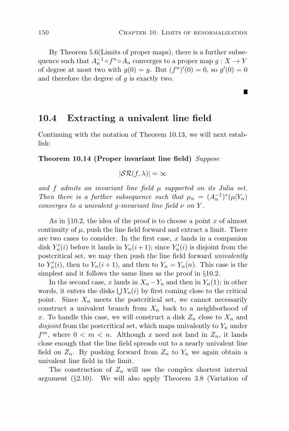
150 Chapter 10. Limits of renormalization
By Theorem 5.6(Limits of proper maps), there is a further subse-quence such that A−1
n fnAn converges to a proper map g : X → Yof degree at most two with g(0) = y. But (fn)′(0) = 0, so g′(0) = 0and therefore the degree of g is exactly two.
10.4 Extracting a univalent line field
Continuing with the notation of Theorem 10.13, we will next estab-lish:
Theorem 10.14 (Proper invariant line field) Suppose
|SR(f,λ)| = ∞
and f admits an invariant line field µ supported on its Julia set.Then there is a further subsequence such that µn = (A−1
n )∗(µ|Yn)converges to a univalent g-invariant line field ν on Y .
As in §10.2, the idea of the proof is to choose a point x of almostcontinuity of µ, push the line field forward and extract a limit. Thereare two cases to consider. In the first case, x lands in a companiondisk Y ′
n(i) before it lands in Yn(i+1); since Y ′n(i) is disjoint from the
postcritical set, we may then push the line field forward univalentlyto Y ′
n(i), then to Yn(i+1), and then to Yn = Yn(n). This case is thesimplest and it follows the same lines as the proof in §10.2.
In the second case, x lands in Xn−Yn and then in Yn(1); in otherwords, it enters the disks
⋃Yn(i) by first coming close to the critical
point. Since Xn meets the postcritical set, we cannot necessarilyconstruct a univalent branch from Xn back to a neighborhood ofx. To handle this case, we will construct a disk Zn close to Xn anddisjoint from the postcritical set, which maps univalently to Yn underfm, where 0 < m < n. Although x need not land in Zn, it landsclose enough that the line field spreads out to a nearly univalent linefield on Zn. By pushing forward from Zn to Yn we again obtain aunivalent line field in the limit.
The construction of Zn will use the complex shortest intervalargument (§2.10). We will also apply Theorem 3.8 (Variation of

10.4. Extracting a univalent line field 151
expansion) to make several geometric bounds. Below, C(λ) denotesa generic constant depending only on λ; different occurrences of C(λ)are not meant to be the same. Distances and lengths, denoted d(·)and ℓ(·), are measured in the hyperbolic metric on C− P (f).
Theorem 10.15 For any n ∈ SR(f)∗,
ℓ(γn) ≤ ℓ(δn) ≤ 2ℓ(γn), andℓ(γn(i)) ≤ ℓ(∂Yn(i)) ≤ ℓ(γn)
in the hyperbolic metric on C− P (f).
Proof. The left inequalities follow from the fact that γn and γn(i)are the geodesic representatives of the isotopy classes δn and ∂Yn(i).
On the other hand, fn maps δn to γn by degree two and fn−i maps∂Yn(i) to γn by degree one, so the inequalities on the right follow fromthe fact that f expands the hyperbolic metric on C− P (f).
Corollary 10.16 For any n ∈ SR(f,λ), δn is contained in a C(λ)-neighborhood of γn and ∂Yn(i) is contained in a C(λ)-neighborhoodof γn(i).
Proof. The curve δn is isotopic to the geodesic γn on C − P (f).By the preceding theorem, the length of δn is bounded above by 2λ,while n ∈ SR(f,λ) implies the length of γn is bounded below by 1/λ.Theorem 2.23 then guarantees every point in δn is within a boundeddistance of γn.
A similar argument applies to ∂Yn(i), using the fact that ℓ(γn(i)) ≥ℓ(γn)/2 > 1/(2λ) by Theorem 9.3.
Theorem 10.17 For any n in SR(f,λ),
∥(fn)′(x)∥ ≤ C(λ) for all x in δn = ∂Xn; and∥(fn−i)′(x)∥ ≤ C(λ) for all x in ∂Yn(i),
with respect to the hyperbolic metric on C− P (f).

152 Chapter 10. Limits of renormalization
Proof. To prove the first inequality, note that fn maps δn to γn bydegree two, so
2ℓ(γn) =∫
δn∥(fn)′(z)∥ ρ(z)|dz|
where ρ(z)|dz| denotes the hyperbolic metric on C − P (f). Sinceℓ(δn) ≥ ℓ(γn), we have ∥(fn)′(x1)∥ ≤ 2 for some x1 in δn.
Any point x2 in δn is joined to x1 by an arc η along δn, suchthat fn(η) is a subarc of γn; in particular, ℓ(fn(η)) ≤ ℓ(γn) < λ. ByTheorem 3.8,
∥(fn)′(x2)∥ ≤ ∥(fn)′(x1)∥α ≤ 2α,
where α depends only on the hyperbolic length of fn(η), and henceis bounded in terms of λ.
Every x in ∂Yn(i) is equal to f i(x′) for some x′ in δn, so the secondinequality follows from the first and the fact that f is an expansion.
Theorem 10.18 For any n ∈ SR(f,λ), there exist i = j such that
d(γn(i), γn(j)) < C(λ)
in the hyperbolic metric on C− P (f).
Proof. Let X ′ be the finite area hyperbolic surface obtained bydeleting from the plane the open disks enclosed by the disjoint simplecurves γn(i). Then X ′ has geodesic boundary
⋃i γn(i) and a single
cusp at infinity. By Theorem 9.3, each boundary component haslength bounded below by L = ℓ(γn)/2 ≥ 1/(2λ). By Theorem 2.24,two boundary components γn(i) and γn(j) are within distance D(L).

10.4. Extracting a univalent line field 153
Theorem 10.19 For n ∈ SR(f,λ), there exists a disk Zn ⊂ C −P (f) and an integer m, 0 < m < n such that
1. fm : Zn → Yn is a univalent map;
2. d(∂Xn, ∂Zn) < C(λ);
3. ℓ(∂Zn) < λ; and
4. area(Zn) > 1/C(λ)
in the hyperbolic metric on C− P (f).
α
f i−1
Yn(j) Yn(i)
Yn(1)
η
W
−Zn−ββ
Zn
f
X
Figure 10.4. Construction of Zn.
Remark. It may be the case Zn meets Xn.
Proof. By the preceding result, there are γn(i) and γn(j) such thatthe hyperbolic distance d(γn(i), γn(j)) bounded in terms of λ. ByCorollary 10.16, Yn(i) is uniformly close to γn(i), so d(Yn(i), Yn(j)) <C(λ) as well. We may assume i < j.
Let α be a geodesic of length less than C(λ) joining ∂Yn(i) and∂Yn(j). (If Yn(i) intersects Yn(j) we take α to be a geodesic of lengthzero.)

154 Chapter 10. Limits of renormalization
The map f i−1 : Yn(1) → Yn(i) is univalent, so it admits a univa-lent inverse
f1−i : Yn(i) → Yn(1).
Since (α ∪ Yn(j)) ∩ P (f) = Pn(j), there is an analytic continuationof this branch of f1−i to a univalent map sending α∪Yn(j) to η∪W ,where η is an arc joining the disk W to Yn(1). Note that W is eitherequal to Yn(j − i+ 1) or it is disjoint from the postcritical set.
Since f(0) lies in Yn(1), the set
W ∪ η ∪ ∂Yn(1)
has a two-fold cover under f equal to
Zn ∪ β ∪ ∂Xn ∪−β ∪−Zn,
where f(Zn) = f(−Zn) = W . (See Figure 10.4.)After possibly replacing Zn by −Zn, we can assume Zn is disjoint
from the postcritical set. (Indeed, if Zn meets P (f), then Zn =Yn(j − i) and −Zn = Y ′
n(j − i) is disjoint from P (f).)Since f i : Zn → Yn(j) and fn−j : Yn(j) → Yn(n) = Yn are
univalent maps, so is fm : Zn → Yn, where m = n+ i− j < n.The map fm is an expansion, so we have
ℓ(∂Zn) ≤ ℓ(γn) < λ.
Similarly, ℓ(β) ≤ ℓ(α), so d(∂Zn, ∂Xn) is bounded in terms of λ.Finally we show there is a lower bound on area(Zn) depending
only on λ. The idea is that fm is not too expanding near ∂Zn, andit maps a neighborhood of ∂Zn to a region of definite area in Yn.
To begin with, let
E1 = z : d(z, γn) < 1 ∩ Yn.
The Collar Theorem 2.18 provides a lower bound (depending on λ)for the injectivity radius of C−P (f) along γn, and therefore a lowerbound on area(E1).
The map fn−j : Yn(j) → Yn is univalent, so there is a regionE2 ⊂ Yn(j) mapping injectively to E1. By Theorems 10.17 and 3.8,we have ∥(fn−j)′(z)∥ < C(λ) in E2, so we obtain a lower bound onarea(E2).

10.4. Extracting a univalent line field 155
Similarly, the map f i : Zn → Yn(j) carries a region E3 ⊂ Zn
injectively to E2. Any point z ∈ E3 can be joined to ∂Xn by anarc η such that ℓ(f i(η)) < C(λ). Indeed, we may arrange that f i(η)consists of a geodesic joining f i(z) to ∂Yn(j), followed by an arcalong ∂Yn(j), followed by β. Thus Theorem 3.8 bounds ∥(f i)′(z)∥in terms of λ and the max of ∥(f i)′∥ along ∂Xn. But the latter isbounded in terms of λ by Theorem 10.17.
Since f i(E3) = E2, we obtain a lower bound on area(E3) in termsof λ, and hence a lower bound on area(Zn).
Proof of Theorem 10.14 (Proper invariant line field). Let x bea point of almost continuity of µ, enjoying the properties guaranteedby Corollary 10.11 for almost every x ∈ J(f).
For each n ∈ SR(f,λ), let k(n) ≥ 0 be the least non-negativeinteger such that fk(n)+1(x) ∈ Yn. Then k(n) → ∞ as n → ∞. Wewill only consider n large enough that k(n) > 0, so fk(n)(x) is not inYn.
Next we construct univalent maps hn : Yn → Tn ⊂ C. We havefk(n)+1(x) ∈ Yn(i(n) + 1) for some i(n) with 0 ≤ i(n) ≤ n − 1.Two cases will be distinguished, depending on whether i(n) > 0 ori(n) = 0.
Case I: i(n) > 0. Then fk(n)(x) ∈ Y ′n(i(n)) (since fk(n)(x) ∈ Yn).
Define hn : Yn → C by the following composition:
Ynf i(n)−n
−−−−→ Y ′n(i(n))
f−k(n)
−−−−→ Tn ⊂ C,
where the univalent branch of f−k(n) is chosen to send fk(n)(x) backto x. This branch is defined on all of Y ′
n(i(n)) because Y ′n(i(n)) is
disjoint from the postcritical set.
Case II: i(n) = 0. Then fk(n)+1(x) ∈ Yn(1) but fk(n)(x) ∈ Yn(n) =Yn. Thus fk(n)(x) ∈ Xn − Yn.
Note that Xn−Yn is disjoint from the postcritical set, since ∂Xn
and ∂Yn are homotopic in C − P (f). By Corollary 10.16, ∂Xn iscontained in a C(λ) neighborhood of ∂Yn, so the same is true of thewhole region Xn − Yn; in particular, the distance from fk(n)(x) to∂Xn is so bounded. By Theorem 10.19, the distance from ∂Xn to

156 Chapter 10. Limits of renormalization
fm
Yn
fk(n)(x)
ζnZn
fk(n)
τn
Tn
Pn
Xn
x
Figure 10.5. Case II: fk(n)(x) ∈ Xn − Yn.
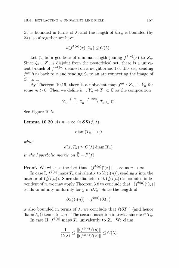
10.4. Extracting a univalent line field 157
Zn is bounded in terms of λ, and the length of ∂Xn is bounded (by2λ), so altogether we have
d(fk(n)(x), Zn) ≤ C(λ).
Let ζn be a geodesic of minimal length joining fk(n)(x) to Zn.Since ζn ∪ Zn is disjoint from the postcritical set, there is a univa-lent branch of f−k(n) defined on a neighborhood of this set, sendingfk(n)(x) back to x and sending ζn to an arc connecting the image ofZn to x.
By Theorem 10.19, there is a univalent map fm : Zn → Yn forsome m > 0. Then we define hn : Yn → Tn ⊂ C as the composition
Ynf−m
−−−→ Znf−k(n)
−−−−→ Tn ⊂ C.
See Figure 10.5.
Lemma 10.20 As n → ∞ in SR(f,λ),
diam(Tn) → 0
whiled(x, Tn) ≤ C(λ) diam(Tn)
in the hyperbolic metric on C− P (f).
Proof. We will use the fact that ∥(fk(n))′(x)∥ → ∞ as n → ∞.In case I, fk(n) maps Tn univalently to Y ′
n(i(n)), sending x into theinterior of Y ′
n(i(n)). Since the diameter of ∂Y ′n(i(n)) is bounded inde-
pendent of n, we may apply Theorem 3.8 to conclude that ∥(fk(n))′(y)∥tends to infinity uniformly for y in ∂Tn. Since the length of
∂Y ′n(i(n)) = fk(n)(∂Tn)
is also bounded in terms of λ, we conclude that ℓ(∂Tn) (and hencediam(Tn)) tends to zero. The second assertion is trivial since x ∈ Tn.
In case II, fk(n) maps Tn univalently to Zn. We claim
1
C(λ)≤ ∥(fk(n))′(y)∥
∥(fk(n))′(x)∥≤ C(λ)

158 Chapter 10. Limits of renormalization
for all y ∈ Tn∪τn. First, the injectivity radius of C−P (f) is boundedbelow (in terms of λ) at fk(n)(x), since this point is within a boundeddistance of the geodesic γn and ℓ(γn) > 1/λ. (Here we use the CollarTheorem 2.18 and the fact that the log of the injectivity radius isLipschitz, by Corollary 2.22.) Secondly, y can be joined to x by anarc η such that
ℓ(fk(n)(η)) ≤ ℓ(ζn) + diam(Zn);
since the latter quantity is bounded in terms of λ, the claim followsfrom the second part of Theorem 3.8.
Since the arc η maps to an arc of bounded length, we have
d(x, y) ≤ C(λ)
∥(fk(n))′(x)∥
for any y in Tn. In particular this shows diam(Tn) → 0 in case II.To check the last condition, we use the fact that the area of Zn is
bounded below in terms of λ (Theorem 10.19). Using the fact thatthe norm of the derivative varies by a bounded factor, we have
1
C(λ)≤ area(Zn) =
∫
Tn
∥(fk(n))′(y)∥2 ρ(y)2|dy|2
≤ C(λ) area(Tn)∥(fk(n))′(x)∥2,
where ρ(y)2|dy|2 denotes the area element of the hyperbolic metricon C − P (f). Now diam(Tn) is bounded in terms of λ, so area(Tn)is bounded by a constant times diam(Tn)2. Thus
1
∥(fk(n))′(x)∥≤ C(λ) diam(Tn).
Combining this the bound d(x, y) ≤ C(λ)/∥(fk(n))′(x)∥ just ob-tained, we conclude that d(x, y) ≤ C(λ) diam(Tn) for any y in Tn.
Lemma 10.21 The map hn extends to a univalent map defined onan annulus of definite modulus about Yn.

10.4. Extracting a univalent line field 159
Proof. By the Collar Theorem 2.18, there is a collar C(γn) of defi-nite modulus with core curve γn, contained in C−P (f). Since C(γn)is disjoint from the postcritical set, any univalent branch of an in-verse iterate of f which is defined on Yn extends to C(γn). The maphn is such an inverse branch.
Completion of the proof of Theorem 10.14 (Proper invariantline field). Consider a sequence of n in SR(f,λ) such that Theorem10.13 holds along this sequence. In particular, (An(Yn), 0) → (Y, 0)in the Caratheodory topology, where An(z) = z/Eucl.diam(Bn) andEucl.diam(·) denotes Euclidean diameter.
Letkn = hn A−1
n : An(Yn) → Tn.
By Theorem 10.12,
1 ≤ Eucl.diam(An(Yn)) ≤ C(λ).
Since kn has a univalent extension to an annulus of definite modulusabout An(Yn), and kn(An(Yn)) = Tn, the Koebe principle implies
1
C(λ)|k′n(0)| ≤ Eucl.diam(Tn) ≤ C(λ)|k′n(0)|.
The Euclidean and hyperbolic metrics are nearly proportional nearx, and the hyperbolic diameter of Tn tends to zero, so |k′n(0)| → 0.Similarly, |x− kn(0)|/|k′n(0)| is bounded in terms of the ratio
d(x, Tn) + diam(Tn)
diam(Tn)
(measured in the hyperbolic metric), and the latter is bounded interms of λ by Lemma 10.20.
Thus Theorem 5.16 implies there is a further subsequence of n inSR(f,λ) such that
νn = k∗n(µ)
converges to a univalent line field ν on (Y, 0) = lim(An(Y ), 0). Buthn is an inverse branch of an iterate of f , so f -invariance of µ impliesνn = (A−1
n )∗µ. Since µ is fn-invariant, the limit ν is g-invariant byTheorem 5.14.

160 Chapter 10. Limits of renormalization
Proof of Theorem 10.9 (Thick rigidity). Suppose
0 < lim infSR(f)∗
ℓ(γn) < ∞.
Then |SR(f,λ)| = ∞ for some λ. If f admits an invariant line fieldµ on its Julia set, then by Theorems 10.13 and 10.14 we obtain aproper map of degree two g : X → Y with g′(0) = 0, 0 ∈ X ∩Y , anda g-invariant univalent line field ν on Y . The presence of a criticalpoint in Y makes this impossible (Theorem 5.13).
Thus f itself admits no measurable invariant line field on its Juliaset.
Proof of Theorem 1.7 (Robust rigidity). If f is robust, thenL = lim inf ℓ(γn) < ∞. If L = 0 then f admits no invariant linefield on its Julia set by Corollary 10.4. The case L > 0 is covered byTheorem 10.9.

Chapter 11
Real quadratic
polynomials
This chapter recapitulates and carries further Sullivan’s a prioribounds for the postcritical set of an infinitely renormalizable realquadratic polynomial [Sul4, §3]. In particular, we show any infinitelyrenormalizable real quadratic polynomial is robust. The main pointis that the order structure of the real line keeps the postcritical setfrom doubling back on itself.
From robustness we deduce the main corollaries stated in theintroduction. We conclude with a generalization to polynomials ofthe form z2n + c.
Remark on bounded type. An infinitely renormalizable quadraticpolynomial with SR(f) = n0 < n1 < n2 < . . . has bounded com-binatorics if supni+1/ni < ∞. For real quadratics with boundedcombinatorics, Sullivan also develops estimates for the quadratic-like renormalizations fn : Un → Vn. These bounds are more difficultand will not be needed here.
11.1 Intervals and gaps
Let f(z) = z2 + c, c ∈ R be a real quadratic polynomial with con-nected Julia set.
161

162 Chapter 11. Real quadratic polynomials
Theorem 11.1 The filled Julia set K(f) meets the real axis in aninterval [−β,β] bounded by the β fixed point of f and its preimage.
Proof. By symmetry with respect to z +→ z and z +→ −z, thefilled Julia set meets the real axis in an interval symmetric about theorigin. The zero ray lies along the positive real axis, so the positiveendpoint of this interval is β.
Theorem 11.2 Every renormalization of a real quadratic polyno-mial f is simple.
Proof. Suppose fn : Un → Vn is a renormalization which is hybridequivalent to g(z) = z2 + c′. One may choose the quasiconformalconjugacy between fn and g to respect the symmetry z +→ z, so c′ isreal and K(g) ∩ R = [−βg,βg], where βg is the β fixed point of g. Itfollows that Kn∩R is bounded by the β fixed point of fn : Kn → Kn
and its preimage. If Kn meets another small Julia set Kn(i), it doesso in a single periodic point x. This x is an endpoint of the intervalKn ∩ R, so x is the β fixed point of Kn and the renormalization issimple.
Definitions. For a bounded subset E ⊂ R we let [E] denote theclosed convex hull of E (the smallest closed interval containing E).For each n ∈ R(f), let
In(i) = [Pn(i)].
Since In(i) lies in the filled Julia set Kn(i), which meets the realaxis in an interval, the interiors of the intervals In(i) at a given levelare disjoint. If f is infinitely renormalizable, the closed intervalsare disjoint as well, since the postcritical set contains no periodicpoints (Theorem 8.1). For i < n, f maps In(i) homeomorphically toIn(i+ 1), while f(In(n)) ⊂ In(1).
The critical interval at level n is In(n), also denoted In. This isthe interval containing the critical point.

11.1. Intervals and gaps 163
Lemma 11.3 Let L(s) ⊃ In(s) be an open interval not contain-ing In(i) for any i < s. Then for t = 1, . . . s there is an intervalL(t) ⊃ I(t) and a branch of f t−s such that f t−s : L(s) → L(t) is ahomeomorphism.
This branch extends to a univalent map f t−s : B(s) → C, whereB(s) is the open Euclidean ball with diameter L(s).
Remark. We emphasize that L(s) can meet In(i) for some i < s.For example, if L(s) is the interior of the convex hull of the intervalsadjacent to In(s), then it satisfies the hypotheses of the lemma.
Proof. We will construct open intervals L(t) ⊃ I(t) for t = 1, . . . s,such that
(i) f maps L(t) homeomorphically to L(t+1) (for t < s);and
(ii) L(t) does not contain In(i) for any i < t.
By assumption L(s) satisfies (ii).Now suppose L(t) has been constructed and t > 1. The critical
value c of f(z) = z2+ c is the most negative point in the postcriticalset (since f(R) = [c,∞)). Therefore (ii) implies c does not lie inL(t) (if it did, In(1) would be contained in L(t).) Thus f−1 has twobranches on L(t), one of which maps L(t) to an interval L(t − 1)containing In(t − 1). Property (ii) for L(t − 1) follows from (ii) forL(t) and the fact that f(In(i)) ⊂ In(i + 1) for any i. Thus we maycontinue the induction until t = 1.
The postcritical set of f lies in R ∪ ∞, so any inverse branchdefined on L(s) can be extended to a univalent map on the upperand lower halfplanes. In particular, we may obtain a univalent mapf s−t : B(s) → C extending the branch f s−t : L(s) → L(t).
Theorem 11.4 (Sullivan) Suppose fn is renormalizable, and letIn(j) denote the interval closest to the critical interval In. Thenthere is a universal λ > 1 such that
|[In(j) ∪ In]| > λ|In|.

164 Chapter 11. Real quadratic polynomials
f
0
In(s)In(j)InIn(1)
cL(s)
f
In(j + 1) −In(j)
Figure 11.1. A definite gap to one side of the critical interval.
The proof is an application of the ubiquitous “shortest intervalargument”.
Proof of Theorem 11.4. Let In(s) be the interval whose Euclideanlength is the shortest among the intervals at level n. Let L(s) be theopen interval symmetric about In(s) and of length |L(s)| = 3|In(s)|.Since In(s) is the shortest interval, L(s) does not contain any otherintervals among the In(i). Thus we may apply Lemma 11.3 to obtaina univalent branch of f1−s defined on B(s) and mapping L(s) toL(1) ⊃ In(1).
The Koebe distortion theorem implies |L(1)| > κ|In(1)| for someuniversal κ > 1. Since L(s) contains no In(i) other than In(s), theinterval L(1) only contains In(1). Therefore the convex hull H ofIn(1) and In(j + 1) satisfies
|H| > κ|In(1)|.
The interval H ′ = f−1(H) is the convex hull of In(j) and −In(j)(see Figure 11.1). Since f−1 is simply a square-root about c, we have
|H ′| >√κ|In|.
The theorem follows, with λ = (1 +√κ)/2.
For a more pictorial proof, see [Sul4, Figures 3 and 4].
Definition. A gap for In(i) is an interval J , disjoint from In(i), suchthat [J ∪ In(i)] is disjoint from In(j) for every j = i. A definite gapis one satisfying |J | > α|In(i)| for a universal constant α > 0.

11.2. Real robustness 165
In what follows, the implicit constant α for one theorem maydepend on that from a preceding result, but since the bounds arederived in order, they are all universal.
Corollary 11.5 If fn is renormalizable, then every interval In(i)has a definite gap to one side.
Proof. The interval −In(j) is disjoint from the postcritical set, sothe critical interval In has a definite gap to one side (see Figure11.1). Let L(n) ⊃ In = In(n) be the interior of [In(j) ∪ −In(j)].Then we may apply Lemma 11.3 to construct intervals L(i) ⊃ In(i)for i = 1, . . . n − 1, and univalently branches of f i−n defined on theball with diameter L(n) and sending L(n) to L(i). Since
⋃ni=1 In(i)
is forward invariant, the preimage of a gap is a gap. By the Koebetheorem, the image under f i−n of the definite gap to one side of thecritical interval gives a definite gap to one side of In(i) for every i.
11.2 Real robustness
To obtain robustness, we need to have definite gaps on both sides ofthe critical interval. In general, however, such gaps are not present atevery level of renormalization. For example, when one tunes f1(z) =z2−1 by an infinitely renormalizable real mapping f2(z) = z2+c withc close to −2, the resulting polynomial f has only a small gap betweenI2(1) and I2(2). This small gap results because the attracting basinsof f1 meet at the α fixed point. The construction cannot be iterated,however, because f2 does not share this property. By this informalreasoning, one expects definite gaps on both sides to appear at leastat every other level of renormalization.
More precisely, we have:
Theorem 11.6 For every n ∈ R(f), either the critical interval Inhas a definite gap on both sides, or j = n/2 ∈ R(f) and Ij has adefinite gap on both sides.

166 Chapter 11. Real quadratic polynomials
Proof. As before, let In(j) denote the interval closest to In. Con-sider the branch of f1−j defined on L(n) = [In(j) ∪ −In(j)] thatmaps the critical interval In to In(n− j+1). Under this branch, theinterval In(j) either maps to a gap, or it maps to In(1), the intervalcontaining the critical value.
In the first case, by applying the Koebe theorem to f1−j, weobtain definite gaps on both sides of In(n − j + 1), since In(j) and−In(j) each have definite length compared to In. Similarly, the ap-propriate branch of fn−j sends the definite gaps for In(n− j +1) todefinite gaps on both sides of In(1); pulling back by one more iterateof f , we obtain definite gaps on both sides of In. This establishesthe theorem in the first case.
In the second case, we have that In(1) and In(n − j + 1) areadjacent intervals among
⋃In(i). Since f maps In to In(1), it maps
In(j) to the interval adjacent to In(1), and thus j + 1 = n − j + 1and j = n/2.
Let Ei = [In(i) ∪ In(i + n/2)] for i = 1, 2, . . . n/2. It is not hardto check that these paired intervals are disjoint, so the sets Ei satisfythe hypotheses of Theorem 8.5, and therefore fn/2 is renormalizable.Moreover Ei = In/2(i).
To conclude, we must show that there is a definite gap on bothsides of In or on both sides of In/2 = [In(n/2)∪ In]. This is not hardto see: if In(n/2) and In are too close together, then there must bedefinite space around In/2.
InG −GIn(n/2)
−In(n/2)In(n/2)K In
Figure 11.2. Definite gaps on both sides.
The argument is explained in Figure 11.2. Let G denote the in-terval between In and In(n/2). By Theorem 11.4, |G| + |In(n/2)|has definite size compared to |In|. If G is large enough, then G and−G provide definite gaps on both sids of In and we are done. Oth-

11.2. Real robustness 167
erwise |G| is much smaller than |In|. In this case |In(n/2)| musthave definite size compared to |In|, so |G| is also much smaller than|In(n/2)|. But then G is too small to serve as the definite gap forIn(n/2) guaranteed by Corollary 11.5. Thus there must be a defi-nite gap K on the other side of In(n/2). Since K has definite sizecompared to In(n/2), and In(n/2) has definite size compared to In,the intervals K and −In(n/2) provide definite gaps on both sides ofIn/2 = [In(n/2) ∪ In].
For the record, here are the constants. By Theorem 11.4,
|G|+ |In(n/2)| = |G|+ |In(j)| > η|In|,
for a universal constant η = λ− 1 > 0. By Corollary 11.5, there is agap of length α|In(n/2)| to one side of In(n/2) for a universal α > 0.
Suppose |G| ≥ α|In(n/2)|. Then we may eliminate |In(n/2)| fromthe inequality above to obtain
|G| > η
1 + 1/α|In|,
so G and −G provide definite gaps on both sides of In.Now suppose |G| < α|In(n/2)|. Then G is too small to serve as
the definite gap for In(n/2), so there is a gap K on the other sideof In(n/2) with |K| > α|In(n/2)|. Moreover the length of In/2 isbounded above in terms of the length of In(n/2):
|In/2| = |In(n/2)|+ |G| + |In| < (1 + 1/η)(|In(n/2)| + |G|)< (1 + 1/η)(1 + α)|In(n/2)|.
If we let ζ = (1 + 1/η)(1 + α), then |In(n/2)| > ζ|In/2| and |K| >αζ|In/2|, so K and −In(n/2) provide definite gaps on both sides ofIn/2.
Corollary 11.7 (Real robustness) If f is an infinitely renormal-izable real quadratic polynomial, then f is robust.
Proof. By Theorem 11.2, all renormalizations of f are simple,so |SR(f)| = ∞. Suppose fn is renormalizable. The hyperbolic

168 Chapter 11. Real quadratic polynomials
geodesic γn in C − P (f) is symmetric about the real axis and sepa-rates the critical interval In from the remaining intervals at level n.A definite gap on both sides of the critical interval gives an upperbound for the hyperbolic length ℓ(γn), by Theorem 2.3. (Alterna-tively, a definite gap gives an annulus of definite modulus in thehomotopy class of γn; then ℓ(γn) is bounded above by the length ofthe core curve of this annulus.)
By Theorem 11.6, once |SR(f)| = ∞ there are infinitely many nin SR(f) such that In has a definite gap on both sides. Thereforelim infSR(f) ℓ(γn) < ∞, so f is robust.
11.3 Corollaries and generalizations
We may now deduce the two main corollaries stated in the introduc-tion:
Corollary 1.8 The Julia set of a real quadratic polynomial carriesno invariant line field.
Corollary 1.9 Every component of the interior of the Mandelbrotset meeting the real axis is hyperbolic.
Proof of Corollaries 1.8 and 1.9. Let f(z) = z2 + c be a realquadratic polynomial.
If f is infinitely renormalizable, then f is robust by Corollary11.7, so by Theorem 1.7 (Robust rigidity) f carries no invariant linefield on its Julia set. On the other hand, a map which is only finitelyrenormalizable carries no invariant line field by Corollary 8.7. Thisproves Corollary 1.8.
Now let U be a component of the interior of the Mandelbrotset meeting the real axis. By the preceding, fc admits no invariantline field on its Julia set for c in U ∩ R. So by Theorem 4.9, U ishyperbolic.
11.3. Corollaries and generalizations 169
Although we have presented our rigidity argument for quadraticpolynomials, many aspects generalize without effort to higher evenexponents; for example one may establish:
Theorem 11.8 If f(z) = z2n + c, n > 1 is an infinitely renormal-izable real polynomial, then f carries no invariant line field on itsJulia set.
However, at present one lacks a rigidity theory for finitely renor-malizable mappings of higher degree (analogous to Theorem 1.6 forquadratic polynomials). It would also be natural to consider poly-nomials with several distinct critical points.

170

Appendix A
Orbifolds
This appendix provides a brief introduction to orbifolds. We beginwith foundational material, including the uniformization theorem forRiemann orbifolds (Theorem A.4). Then we describe the orbifold Of
of a rational map f , and use it to discuss certain critically finite maps.
A.1 Smooth and complex orbifolds
An orbifold is a space which is locally modeled on the quotient ofan open subset of Rn by the action of a finite group. For a generaldevelopment see [Th1, §13]. We will need only the theory of smoothtwo dimensional orbifolds, and their complex analogues which gen-eralize Riemann surfaces. Our definitions will take advantage of thesimplifications possible in this case.
Definition. A smooth n-dimensional orbifold O is a Hausdorff topo-logical space X together with an atlas < Uα, Vα,Γα,φα >, where
1. < Uα > is an open covering of X, providing a base for thetopology on X;
2. < Vα > is a collection of open subsets in Rn;
3. Γα is a finite group of diffeomorphisms of Vα; and
4. φα : Vα → Uα is a continuous map whose fibers are the orbitsof Γα.
171

172 Appendix A. Orbifolds
This atlas is required to satisfy the following compatibility con-dition. Whenever Uα ⊂ Uβ, there exists an injective homomorphismHαβ : Γα → Γβ and a smooth embedding φαβ : Vα → Vβ such that:
1. for all γ ∈ Γα and z ∈ Vα, we have φαβ(γz) = Hαβ(γ)φαβ(z);and
2. for all z ∈ Vα, φβ(φαβ(z)) = φα(z).
The space X is called the underlying space of the orbifold O.A complex n-orbifold is defined by requiring that the charts Vα lie
in Cn, the transition functions φαβ are holomorphic and the groupsΓα act biholomorphically.
Recall that a Riemann surface is a connected complex 1-manifold.Similar, we define a Riemann orbifold to be a connected one-dimen-sional complex orbifold.
Two atlases define the same orbifold structure if their union liesin a third atlas (satisfying the compatibility condition).
The sets Vα form the charts for the orbifold. Just as for a mani-fold, one studies local properties on an orbifold by passing to charts.
Specifying complex 1-orbifolds. A one-dimensional complexorbifold is conveniently specified by a pair (X,N) of a complex 1-manifold X and a multiplicity map
N : X → N,
such thatx ∈ X : N(x) > 1
is discrete. To construct an orbifold from this data, consider thecollection of all conformal isomorphisms ψα : ∆ → Uα ⊂ X suchthat N(ψα(z)) = 1 for all z in ∆ except possibly z = 0. Set Vα = ∆and define φα(z) = ψα(zn), where n = N(ψα(0)). We then take Γα
to be the group generated by z +→ exp(2πi/n)z acting on the disk,and the transition functions are determined in a straightforward way.
Every complex 1-orbifold O is specified in this manner. Indeed,a complex 1-orbifold O determines a complex manifold structure onthe underlying surface X, because the quotients Vα/Γα carry naturalcomplex structures. The orbifold also determines a map N : X → N
as follows: for x ∈ Uα, choose y in Vα such that φα(y) = x, and

A.2. Coverings and uniformization 173
set N(x) equal to the cardinality of the stabilizer of y in Γα. It iseasy to verify that N(x) is well-defined, and that the original orbifoldstructure is equivalent to the one determined by the pair (X,N).
Similarly, every orientable 2-dimensional orbifold is specified bya pair (X,N) where X is a smooth surface and N : X → N assumesvalues greater than one only on a discrete set. (Here orientable meansthere is an atlas such that the group actions and transition functionspreserve orientation.)
A useful convention is to allow N(x) to assume the value ∞ at adiscrete set of points; these points are then omitted from the orbifold,so (X,N) = (Y,N |Y ) where Y = x : N(x) < ∞.
Definitions. Let O = (X,N) be a complex 1-orbifold. The singularpoints of O are those x ∈ X with N(x) > 1. The multiplicity of asingular point x is N(x). The signature of an orbifold is the list ofvalues that N assumes at the singular points; a given value n is re-peated as many times as the number of singular points of multiplicityn.
Traditional complex 1-manifolds will be regarded as orbifoldswith N(x) = 1 everywhere.
A.2 Coverings and uniformization
In this section we treat holomorphic maps and covering maps betweencomplex 1-orbifolds, and discuss the uniformization theorem.
Definitions. Let f : X → X ′ be a holomorphic map betweencomplex 1-manifolds. The local degree deg(f, x) is equal to one morethan the order to which f ′ vanishes at x. Thus deg(zn, 0) = n. (Byconvention the local degree is zero if f is locally constant at x.)
Let O = (X,N) and O′ = (X ′, N ′) be complex 1-orbifolds. Aholomorphic map from O to O′ is a holomorphic map f : X → X ′
between the underlying complex manifolds such that:
N(f(x)) divides deg(f, x)N(x) for each x in X.
This condition is equivalent to the following local lifting property.Whenever x′ = f(x), there exist:
1. neighborhoods Uα and U ′α of x and x′;

174 Appendix A. Orbifolds
2. charts φα : Vα → Uα and φ′α : V ′α → U ′
α; and
3. a holomorphic map g : Vα → V ′α; such that
4. f(φα(z)) = φ′α(g(z)) for all z in Vα.
A holomorphic map f : O → O′ is a covering map if N(f(x)) =deg(f, x)N(x) for all x, and for every neighborhood U ′
α of x′, everycomponent of f−1(U ′
α) maps surjectively to U ′α. Equivalently, the
local lifting property can be verified using the same U ′α for every x
with f(x) = x′, and g : Vα → V ′α can be chosen to be an embedding.
Now suppose O = (X,N) is connected. The Euler characteristicof O is given by
χ(O) = χ(X)−∑
X
(1− 1
N(x)
).
For an orbifold χ(O) is a rational number which may or may not bean integer. Intuitively, each point with N(x) > 1 contributes only1/N(x) to the number of 0-cells inX. The Euler characteristic is −∞if π1(X) is infinitely generated or if X has infinitely many singularpoints.
The Euler characteristic satisfies χ(O) = deg(f)χ(O′) for anyfinite degree covering map between orbifolds.
Theorem A.1 Let Y be a Riemann surface, and let Γ ⊂ Aut(Y )be a group of automorphisms acting properly discontinuously. ThenX = Y/Γ carries a natural orbifold structure such that the projectionY → O = (X,N) is a covering map.
Proof. By proper discontinuity and removability of isolated singu-larities, X = Y/Γ carries a Riemann surface structure such that theprojection π : Y → X is holomorphic. Set N(x) equal to the cardi-nality of the stabilizer of y, where π(y) = x. Since N(x) = deg(π, y),the projection to O = (X,N) is a covering map of orbifolds.

A.2. Coverings and uniformization 175
Theorem A.2 (Uniformization) Let O be a Riemann orbifold.Then exactly one of the following holds:
1. O is covered by C. Equivalently, O is isomorphic to C orto a sphere with signature (n, n), (2, 2, n), (2, 3, 3), (2, 3, 4) or(2, 3, 5), where 1 < n < ∞.
2. O is covered by C. Equivalently, O is isomorphic to C, C∗,a complex torus, or a sphere with signature (n,∞), (2, 2,∞),(2, 3, 6), (2, 4, 4), (3, 3, 3) or (2, 2, 2, 2).
3. O is covered by H. Equivalently, χ(O) < 0 or O is isomorphicto an annulus of finite modulus, the unit disk, the puncturedunit disk, a unit disk with signature (n), n > 1, or a unit diskwith signature (2, 2).
4. O is not covered by any Riemann surface. Equivalently, Ois isomorphic to a sphere with signature (n) or (n,m) where1 < n < m < ∞.
Proof. The universal covering orbifold U of O = (X,N) is con-structed in [Th1, Theorem 13.2.4] by taking an inverse limit of fiberproducts of covering spaces of O; it is unique up to isomorphism overO. If U has no singular points, it is isomorphic to C, C, or H by theclassification of simply-connected Riemann surfaces. On the otherhand, if U does have singular points then O is not covered by anyRiemann surface.
This shows exactly one of cases 1-4 holds. We now verify theequivalent formulations of these cases.
Singular case. The universal cover fails to be a Riemann surface ifand only if O is a sphere with signature (n) or (n,m), 1 < n < m <∞. Indeed, if O is noncompact, then for any x in the singular locusa peripheral loop around x represents a nontrivial homology class inH1(X − x,R), so there is a finite regular covering orbifold of Owhere all the preimages of x are nonsingular. It follows that U hasno singular points.
When O is compact, it has a finite covering which is a Riemannsurface, apart from the examples enumerated in case 4. This ob-servation goes back to Bundgaard, Nielsen and Fox; compare [Nam,

176 Appendix A. Orbifolds
Theorem 1.2.15]. Thus the universal cover of O is also a Riemannsurface.
It is easy to see directly that the examples in case 4 are notcovered by any Riemann surface.
Elliptic case. Suppose the universal covering is given by π : C → O.The group of deck transformations Γ ⊂ Aut(C) consists of thoseautomorphisms such that π γ = π; since C is compact, Γ has finiteorder. Up to conjugacy, Γ is a cyclic group, a dihedral group, or thegroup of symmetries of a regular tetrahedron, cube or dodecahedron.These groups give orbifolds with signatures (n, n), (2, 2, n), (2, 3, 3),(2, 3, 4) and (2, 3, 5) respectively. Conversely, any orbifold with thesemultiplicities is covered by C, because any two triples of points on C
are equivalent by a Mobius transformation.
Parabolic case. Suppose O is covered by C. The group of decktransformations Γ ⊂ Aut(C) acts properly discontinuously on C, soits subgroup Γ′ of translations is normal and of finite index in Γ.Thus O admits a finite regular covering by Z = C/Γ′, where Z isisomorphic to C, C∗ or a complex torus.
If Z = C then Γ is generated by a single rotation and X = C
with at most one singular point.
If Z = C∗, then X = C∗ with no singular points or X is isomor-phic to the quotient of Z by z +→ 1/z, which gives C with singularpoints of multiplicities (2, 2).
If Z = C/Γ′ is a torus, then typically the only non-translationautomorphism of Z is conjugate to z +→ −z; this gives X = C withmultiplicities (2, 2, 2, 2). One exception arises when Γ′ is isomorphicto Z⊕Zi; then the quotient by z +→ iz gives X = C with multiplicities(2, 4, 4). Two others arise when Γ′ is isomorphic to Z⊕Zω, where ωis a primitive sixth root of unity; then the quotient by z +→ ωz givesmultiplicities (2, 3, 6), and the quotient by z +→ ω2z gives (3, 3, 3).
The above discussion shows each of these orbifolds is indeed cov-ered by C, using the fact that any two triples of points on C areequivalent and any two-fold cover of C branched over four points isa torus.
Hyperbolic case. All Riemann orbifolds appearing in the precedingdiscussion have non-negative Euler characteristic. Thus all orbifolds

A.3. The orbifold of a rational map 177
with negative Euler characteristic, and all remaining Riemann orb-ifolds with non-positive Euler characteristic must be covered by H.These remaining orbifolds are enumerated in case 3.
Metrics on complex 1-orbifolds. A smooth Riemannian metric ρon a complex 1-orbifold O = (X,N) is specified by a smooth metricρα on each chart Vα, invariant under the action of Γα and compatibleacross charts. A smooth metric on O determines a singular metric onthe complex manifold X. This metric has a singularity of the type
ρ =|dz|
|z|1−1/n
near a singular point z = 0 of multiplicity n on X.
Definitions. A Riemann orbifold is elliptic, parabolic or hyperbolicif it is covered by C, C or H respectively.
Such an orbifold inherits a spherical, Euclidean or hyperbolicmetric from its universal cover. In the spherical and hyperbolic cases,this metric is uniquely determined by normalizing the curvature to±1. In the Euclidean case, the metric is well-defined up to a positivescalar multiple.
The Schwarz Lemma immediately generalizes to:
Theorem A.3 Let f : O → O′ be a holomorphic map between hy-perbolic orbifolds. Then f does not increase the hyperbolic metric,and f is an infinitesimal isometry if and only if f is a covering map.
A.3 The orbifold of a rational map
In §3 we introduced the hyperbolic metric on C − P (f) as a fun-damental tool for studying the dynamics of a rational map f . Forexample, letting Q(f) = f−1(P (f)), we observed that the restriction
f : (C −Q(f)) → (C− P (f))
is a covering map, hence an isometry for the hyperbolic metric, while
(C −Q(f)) → (C− P (f))

178 Appendix A. Orbifolds
is holomorphic, hence a contraction. Putting these facts together,we saw that f expands the hyperbolic metric on C− P (f).
Orbifolds provide a refinement of this tool that is especially suitedto rational maps with preperiodic critical points in the Julia set. Wewill construct orbifolds Of and Qf such that f : Qf → Of is acovering, and the inclusion Qf → Of is holomorphic. This methodappears in [DH1, §III.7] and is developed systemically for criticallyfinite maps in [Th2].
Definition. Let f : C → C be a rational map of degree d > 1 withpostcritical set P (f). The orbifold Of = (Xf , Nf ) of f is a complex1-orbifold constructed as follows. First, Xf is obtained by deleting
from C every non-isolated point of P (f). Then, for each x in Xf , wedefine Nf (x) to be the least common multiple of the local degrees
deg(fn, y) for all n > 0 and all y ∈ C such that fn(y) = x. Byconvention Nf (x) = ∞ if these local degrees are unbounded; thishappens if and only if x belongs to a periodic cycle containing acritical point.
Note thatC− P (f) ⊂ Xf
and Nf (x) = 1 for every x outside P (f), so this inclusion is a holo-morphic map of orbifolds.
Example. Let f(z) = z2 + i; then Xf = C, Nf (∞) = ∞, Nf (i) =Nf (−1 + i) = Nf (−i) = 2, and Nf = 1 at all other points.
Now let Qf = (Yf , N ′f ) where Yf = f−1(Xf ) and N ′
f (y) is theinteger Nf (f(y))/deg(f, y). It is easy to see
f : Qf → Of
is a covering map, while the inclusion
Qf → Of
is holomorphic as a map of orbifolds. This easily implies:
Theorem A.4 Exactly one of the following holds:
1. The orbifold Of is connected and parabolic, f : Of → Of is acovering map, and ∥f∥ = C > 1 in the Euclidean metric onOf .

A.3. The orbifold of a rational map 179
2. Every component of Of is hyperbolic, and ∥f ′(x)∥ ≥ 1 withrespect to the hyperbolic metric on Of when x and f(x) bothlie in Of .
Proof. Suppose Of is connected. Then
χ(Of ) ≥ χ(Qf ) = deg(f)χ(Of ),
so χ(Of ) ≤ 0. If χ(Of ) = 0, then Of is parabolic and the equalitymust hold above, which implies Qf = Of and f : Of → Of is acovering map. The map f lifts to z +→ αz on the universal cover C ofOf , where C = |α| > 1 because the degree of f is greater than one.Thus f expands the Euclidean metric on Of by the constant C.
If χ(Of ) < 0 or Of is disconnected, then every component of Of
is hyperbolic and ∥f ′∥ ≥ 1 by the Schwarz Lemma.
Rational maps with parabolic orbifolds are classified in [Th2] and[DH3]. A rich class of such examples are associated to the torusendomorphisms studied in §3.5, by the following result:
Theorem A.5 If Of is a sphere with signature (2, 2, 2, 2), then f isdouble covered by a torus endomorphism.
Proof. The orbifold Of has a canonical two-fold covering space Twhich is a complex torus. (The torus T is just the two-fold branchedcovering of C branched along P (f). It can also be defined as thequotient of the universal cover C of Of by those deck transformationswhich act as translations.)
Since f : Of → Of is a covering map, it lifts to an endomorphismof T .
Example. Let f(z) = (z2 +1+√2)/(z2 − 1−
√2). Then Of is the
sphere with singular points of multiplicity two at 1, −1, 1 +√2 and
−1 −√2. The map f is covered by the endomorphism z +→ 2iz on
the torus T = C/(Z⊕ Z√2i).
This example shows f need not be covered by an integral torusendomorphism.

180 Appendix A. Orbifolds
Theorem A.6 Let f be a critically finite rational map. Then eachperiodic cycle of f is repelling or superattracting. If f has no super-attracting cycles then J(f) = C.
Proof. The hypotheses imply Of is a connected orbifold of finite Eu-ler characteristic, uniformized by the Euclidean or hyperbolic plane.If Of is parabolic, then ∥f ′∥ = C > 1 with respect to the Euclideanmetric on Of . If Of is hyperbolic, then
χ(Qf ) = deg(f)χ(Of ) < χ(Of ) < 0,
so the inclusion Qf → Of is not a covering map; by the SchwarzLemma, we have ∥f ′∥ > 1 pointwise with respect to the hyperbolicmetric on Of .
In either case there is a Riemannian metric on Of which is ex-panded by f , so each periodic cycle in Of is repelling. Any periodiccycle which does not lie in Of must contain a critical point, so it issuperattracting.
In the absence of superattracting cycles, Of is a compact orbifold(whose underlying space is the sphere), so we have uniform expansionin the orbifold metric. Thus the iterates of f cannot form a normalfamily at any point and the Julia set of f is C.
Compare [Th2, §13].The preceding two theorems were used in §3.

Appendix B
A closing lemma for
rational maps
In this appendix we develop the idea of a quotient of a rational map.A quotient is obtained by collapsing pieces of the postcritical set tosingle points, to yield a simpler branched covering of the sphere. Wewill show that when the postcritical set of the quotient is finite, thequotient branched covering can also be realized as a rational map.
Another way to look at our main result is that it provides aclosing lemma for rational maps — that is, a method for findinga new dynamical system where a recurrent critical orbit becomesperiodic. Our result will not guarantee that the closed dynamicalsystem is near the original one, however.
For quadratic polynomials, there is a close relationship betweenquotients and renormalization. For example, we will associate to anyinfinitely renormalizable quadratic polynomial f an infinite sequencegn of critically finite quotients. Conjecturally, these quotients gnconverge to the original map f . This conjecture implies the densityof hyperbolic dynamics in the quadratic family.
B.1 Quotients of branched coverings
Definitions. To discuss the closing lemma, we introduce a cate-gory whose objects are branched coverings of the sphere and whosemorphisms are combinatorial quotient maps.
181

182 Appendix B. A closing lemma for rational maps
Spheres with marked points. Let (S2, A) denote the sphere witha distinguished closed subset A. A quotient map
φ : (S2, A) → (S2, B)
is a continuous, degree one map such that φ(A) = B, φ−1(b) isconnected for all b in B, and φ−1(x) is a single point for all x inS2 − B. This means A is contained in a set obtained by “blowingup” points of B to (nonseparating) continua.
Two quotient maps φ0 and φ1 are homotopic if there is a contin-uous family φt of quotient maps connecting them, such that φt|A =φ0|A = φ1|A.
A combinatorial quotient map is a homotopy class of quotientmappings. We obtain the category of spheres with marked points bytaking the pairs (S2, A) as objects and combinatorial quotient mapsas morphisms.
It is well-known that if |A| = |B| < ∞, then any combinatorialquotient map φ : (S2, A) → (S2, B) is represented by a homeomor-phism, so these two objects are isomorphic. Similarly, the groupof automorphisms of (S2, A) is equal to the mapping class group ofS2 −A if |A| is finite.
We will use φ to denote both a combinatorial quotient map and atypical representative of its homotopy class, so long as the discussionis independent of the choice of representative.
Branched coverings. Let f : S2 → S2 be a branched covering ofthe sphere; this means that f is a smooth map whose behavior islocally modeled on that of z +→ zd for some d ≥ 1. The integer d isthe local degree of f at x, denoted deg(f, x).
A rational map on the Riemann sphere is a special case of abranched covering.
The set of points with local degree greater than one form the crit-ical points C(f). The postcritical set P (f) is closure of the forwardorbits of the critical points:
P (f) =⋃
c∈C(f), n>0
fn(c).
Note that the critical points need not belong to the postcritical set.We will be concerned exclusively with branched coverings f of degreetwo or more, in which case |P (f)| ≥ 2.

B.1. Quotients of branched coverings 183
A branched covering is critically finite if the |P (f)| < ∞.
Quotients and equivalence of branched coverings. Let f and gbe two branched coverings on the sphere, and let φ be a combinatorialquotient map
φ : (S2, P (f)) → (S2, P (g)).
Suppose there are maps φ0 and φ1 in the homotopy class φ makingthe diagram
S2 φ1−−−→ S2
f
3 g3
S2 φ0−−−→ S2
commutative. In this case we say that g is a quotient of f , and write
φ : f → g.
We can then form the category of branched coverings of the spherewhose objects are branched coverings f and whose morphisms arecombinatorial quotient maps as above.
The map g is a proper quotient of f if |φ−1(x) ∩ P (f)| > 1 forsome x in P (g). This means at least two points of P (f) are collapsedto form a single point of P (g).
Combinatorial equivalence. Thurston defined two critically finitebranched coverings f and g to be combinatorially equivalent if thereare homeomorphisms φi : (S2, P (f)) → (S2, P (g)), i = 0, 1, such thatthe diagram above commutes, and φ0 is isotopic to φ1 rel (P (f), P (g))[Th2], [DH3]. Alternatively, f and g are combinatorially equivalentif after deforming f by isotopy rel P (f), it becomes topologicallyconjugate to g. Using techniques from the mapping class groups ofsurfaces, it can be shown that Thurston’s notion of combinatorialequivalence agrees with isomorphism in the category of branchedcoverings introduced above.
Thus we will use the term combinatorial equivalence to denoteisomorphism in this category.
We can now formulate our main result.
Theorem B.1 (Rational quotients) Let g be a critically finite quo-tient of a rational map f . Then g is combinatorially equivalent to arational map.

184 Appendix B. A closing lemma for rational maps
B.2 Critically finite rational maps
The proof of Theorem B.1 is an application of Thurston’s charac-terization of critically finite rational maps. To state this characteri-zation, we introduce the orbifold associated to a branched coveringand the eigenvalue of an invariant curve system.
The orbifold of a branched cover. Let f : S2 → S2 be acritically finite branched covering. As we did for rational maps in§A.3, we will define a smooth orbifold canonically associated to f .
For each x ∈ S2 define Nf (x) (which may be ∞) as the leastcommon multiple of the local degrees deg(fn, y) for all n > 0 and ally in S2 such that fn(y) = x. (Note that Nf (x) = 1 if x is not in thepostcritical set P (f).) Then Of = (S2, Nf ) is orbifold of f .
The eigenvalue of a curve system. A simple closed curve γ onS2 − P (f) is essential if it does not bound a disk in S2 − P (f). Acurve is peripheral if it encloses a single point of P (f). Two simplecurves γ and δ are parallel if they are isotopic in S2 − P (f).
A curve system Γ = γi on S2 − P (f) is a finite nonemptycollection of disjoint simple closed curves, each essential and nonpe-ripheral, and no two parallel. A curve system determines a transitionmatrix A(Γ) : RΓ → RΓ by the formula
Aγδ =∑
α
1
deg(f : α→ δ)
where the sum is taken over components α of f−1(δ) which are iso-topic to γ.
Let λ(Γ) ≥ 0 denote the spectral radius of A(γ). Since A(Γ) ≥ 0,the Perron-Frobenius theorem guarantees that λ(Γ) is an eigenvaluefor A(Γ) with a non-negative eigenvector [Gant, §XIII].
A curve system is f -invariant if for each γ in Γ, each componentα of f−1(γ) is either inessential, peripheral or parallel to a curve inΓ.
Theorem B.2 (Thurston) Let f : S2 → S2 be a critically finitebranched covering. Then f is combinatorially equivalent to a rationalmap g if and only if:
(Torus case) Of has signature (2, 2, 2, 2) and g is double coveredby a torus endomorphism; or

B.2. Critically finite rational maps 185
(General case) Of does not have signature (2, 2, 2, 2) and
λ(Γ) < 1
for every f -invariant curve system Γ on S2 − P (f).In the second case, g is unique up to conformal conjugation.
For a proof, see [Th2], [DH3].
Remark. In the torus case, f lifts to a covering map f : X → Xwhere X is a torus double covering Of . (Compare Theorem A.5.)Then f is equivalent to a rational map if and only if the inducedlinear map
f∗ : H1(X,R) → H1(X,R)
is conformal with respect some metric on H1(X,R) ∼= R2. Equiv-alently, if we represent f∗ by a 2 × 2 integer matrix
(a bc d
), then f
is combinatorially a rational map if and only if the correspondingMobius transformation z +→ (az + b)/(cz + d) has a fixed point inthe upper halfplane. Thus we have a combinatorial criterion for ra-tionality in the torus case as well as in the general case.
In the torus case, H is the Teichmuller space of conformal struc-tures on Of , pullback of structures by f determines a map of Te-ichmuller space to itself, and f is combinatorially rational if andonly if this map has a fixed point. The general case is analyzed bya similar method, using the Teichmuller space of the sphere with|P (f)| marked points.
To show that a critically finite quotient g of a rational map f isitself rational (Theorem B.1), the basic idea is to check that g inheritsthe property λ(Γ) < 1 from f and apply Thurston’s criterion. Thereare two important details to take care of:
1. The rational map f might admit an invariant curve systemwith λ(Γ) = 1.
2. The orbifold Og of the branched covering g might have signa-ture (2, 2, 2, 2).
These details are addressed in the next two sections to completethe proof of Theorem B.1 (Rational quotients).

186 Appendix B. A closing lemma for rational maps
B.3 Siegel disks, Herman rings and curve sys-
tems
In this section we consider a rational map f whose postcritical setmay be infinite, and classify all the examples which admit a curvesystem Γ with λ(Γ) = 1.
We will not require that Γ is f -invariant. Although Thurston’stheorem makes reference only to invariant curve systems, it is tech-nically convenient to forgo this assumption.
Theorem B.3 Let f(z) be a rational map, and let Γ be a curvesystem on C− P (f). Then λ(Γ) ≤ 1.
Theorem B.4 (Classification of λ(Γ) = 1) Let Γ be a curve sys-tem for a rational map f . If λ(Γ) = 1, then either:
1. f is critically finite, Of is the (2, 2, 2, 2) orbifold and f is doublecovered by an integral torus endomorphism; or
2. |P (f)| = ∞, and Γ includes the essential curves in a finitesystem of annuli permuted by f . These annuli lie in Siegeldisks or Herman rings for f , and each annulus is a connectedcomponent of C− P (f).
Definitions. Disjoint annuli A1, . . . An on the sphere are nested ifthere are two points which are separated by every Ai. The join ofa nested sequence, denoted join(A1, . . . , An), is the smallest annuluscontaining every Ai as an essential subannulus. Its boundary consistsof a one component from the boundary of the “innermost” annulusand another from the “outermost” annulus.
Theorem B.5 If B = join(A1, . . . , An) is the join of a set of nestedannuli of finite moduli, then
mod(B) ≥∑
mod(Ai).
Equality holds if and only if in a conformal coordinate where B =z : 1 < |z| < R, each Ai has the form
Ai = z : ri < |z| < si,
and the Ai fill all of B except for a finite number of circles.
B.3. Siegel disks, Herman rings and curve systems 187
This proposition is a sharp form of superadditivity of the modulus[LV, §I.6.6].
Now let Γ be a curve system with transition matrix Aγδ . We sayΓ is irreducible if for any (γ, δ) there is an n > 0 such that An
γδ > 0.The Perron-Frobenius theory easily implies [Gant, §XIII.4]:
Theorem B.6 Any curve system with λ(Γ) > 0 contains an irre-ducible curve system Γ′ with λ(Γ) = λ(Γ′).
Thus in the proofs of Theorems B.3 and B.4 we will assume thatΓ is irreducible.1
Both proofs involve the study of systems of disjoint simple annuliCγ representing the isotopy classes Γ on C−P (f). From any systemof annuli Cγ , γ ∈ Γ, we can construct a new system of pullback annuliC ′γ by setting
C ′γ = join(D1, . . . ,Dn),
where Di enumerates the set of components of f−1(⋃
δ∈Γ Cδ) which
are isotopic to γ in C−P (f). (This set is nonempty by irreducibility).We denote this pullback operation by
C ′ = f∗C.
Theorem B.7 The moduli of the pullback annuli satisfy
mod(C ′γ) ≥
∑
γ
Aγδ mod(Cδ).
Proof. If an annulus A′ covers an annulus A with degree d, thenmod(A′) = mod(A)/d; the proposition follows from this fact, super-additivity of the modulus and the definition of the transition matrix.
1The property of f -invariance may be lost in passing to Γ′, which is one reasonwe do not require invariance.

188 Appendix B. A closing lemma for rational maps
Proof of Theorem B.3. The proof follows the same lines as partof Thurston’s result (Theorem B.2). There are constants Mγ suchthat
mod(Cγ) ≤ Mγ
for any annulus system representing Γ; for example, if X is the com-ponent of C − P (f) containing γ, we may choose Mγ equal to themodulus of the covering space of X determined by the cyclic sub-group ⟨γ⟩ ⊂ π1(X). Starting with any annulus system C0, defineinductively Cn+1 = f∗Cn. Since the modulus of Cn
γ is boundedabove, the iterates of A applied to the positive vector [mod(C0
γ)] arebounded as well, so λ(Γ) ≤ 1.
Now assume λ(Γ) = 1. To analyze this case, it is useful to choosethe annuli Cγ as large as possible, using:
Theorem B.8 (Strebel) Let Γ be a nonempty set of disjoint sim-ple geodesics on a (connected) hyperbolic Riemann surface X withassigned weights mγ > 0. Then there exists a unique collection of dis-joint open annuli Cγ representing the isotopy classes Γ and maximiz-ing
∑mod(Cγ), subject to the condition that the moduli [mod(Cγ)]
are proportional to [mγ ].
From uniqueness one may easily show:
Corollary B.9 If C ′γ is another system of disjoint annuli represent-
ing Γ, such that mod(C ′γ) ≥ mod(Cγ) for all γ, then C ′
γ = Cγ .
See [Str, Theorems 20.6 and 21.7].Now let mγ > 0 be a positive solution to the eigenvalue equa-
tion Am = m; such a solution exists by irreducibility. ApplyingStrebel’s theorem, we will construct a canonical system of annuli Cγ
representing the curves Γ, and with [mod(Cγ)] proportional to [mγ ].More precisely, we define Cγ as the unique system of annuli such
that
(a)∑
mod(Cγ) is maximized, subject to the condition:
(b) mod(Cγ)/mod(Cδ) = mγ/mδ whenever γ and δ lie
in the same component of C− P (f).

B.3. Siegel disks, Herman rings and curve systems 189
Although we have only applied Strebel’s result component by com-ponent, we have:
Theorem B.10 Assuming Γ is irreducible, there is a constant c > 0such that mod(Cγ) = cmγ for all γ.
Proof. Write mod(Cγ) = cmγ + vγ , where c > 0, vγ ≥ 0 and vα = 0
for some particular curve α lying in a component X of C − P (f).Then by construction, mod(Cγ) = cmγ for every γ lying in X.
We will show v = 0. If not, we can choose n such that (Anv)α > 0by irreducibility. Then C ′ = (fn)∗(C) satisfies mod(C ′
α) > mod(Cα)and mod(C ′
γ) ≥ mod(Cγ) for all γ lying inX, contradicting CorollaryB.9.
Corollary B.11 The maximal annuli are invariant under pullback:if C ′ = f∗C, then C ′
γ = Cγ for all γ ∈ Γ.
Proof. Since Am = m, the moduli of the pullback annuli satisfymod(C ′
γ) ≥ mod(Cγ); thus the two systems of annuli are equal bythe uniqueness part of Strebel’s theorem (Corollary B.9).
Definition. Let D = f−1(⋃
ΓCγ). An amalgam A is an annulus in
C such that A = join(D1, . . . ,Dn), and mod(A) =∑
mod(Di), forsome collection D1, . . . ,Dn of nested components of D. It followsthat adjacent Di are separated by real analytic circles as in TheoremB.5. Note that the Di’s may represent distinct homotopy classes onC− P (f).
Since mod(Cγ) =∑
Aγδ mod(Cδ) =∑
mod(Di), where the lastsum is over the components of D homotopic to γ, we have:
Theorem B.12 Every annulus Cγ is an amalgam.
Theorem B.13 Let A be an amalgam which does not meet the crit-ical points C(f). Then f(A) is an amalgam and the map A → f(A)is a covering map.

190 Appendix B. A closing lemma for rational maps
C2
C1
D2
D1
f
Figure B.1. An unbranched image of an amalgam is an amalgam.
Proof. Let A be an amalgam of D1, . . . Dk. Then f maps each Di
by a covering map to Ci, one of the original annuli Cγ . If there areno critical points on the circles separating adjacent Di’s, then theCi’s are disjoint and nested, so A maps to f(A) by a covering map(see Figure B.1). Then mod(f(A)) =
∑mod(Ci), and since each Ci
is an amalgam, so is f(A).
Theorem B.14 Let A be an amalgam which meets the critical pointsC(f), and let B1, B2 denote the components of ∂A. Then there areamalgams A1, A2 in A, disjoint from C(f), such that ∂f(Ai) =f(Bi) 4 Ii where I1, I2 are real analytic intervals, and the endpointsof Ii lie in the postcritical set P (f).
Proof. Let A = join(D1, . . . Dn); since each Di maps by a coveringmap, the critical points of f must be contained in the circles sepa-rating adjacent Di’s. Let Ai be the maximal amalgam in A disjointfrom C(f) and containing Bi as one of its boundary components.(This Ai is the join of one or more adjacent Di’s lying near one endof A.)
Consider the circle Si forming the other boundary componentof Ai; it necessarily meets the critical points of f . The circle Si is

B.3. Siegel disks, Herman rings and curve systems 191
I1
C2
C1
S1
D2
D1
f
Figure B.2. A branched image of an amalgam, bounded by an interval.
a component of f−1(C −⋃Cγ), so it is a branched cover of f(Si).
Therefore f(Si) = Ii, an interval whose endpoints are critical values(see Figure B.2). By the preceding result, Ai → f(Ai) is a finitecovering map, hence proper, so
∂f(Ai) = f(∂Ai) = f(Bi) 4 f(Si).
Proof of Theorem B.4 (Classification of λ(Γ) = 1). Supposethere exists an annulus Cγ whose iterates An = fn(Cγ) are disjointfrom the critical points of f for all n ≥ 0. Then each An is anamalgam, f carries An to An+1 by a covering map, and mod(An+1) ≥mod(An). There are only finitely many possible amalgams, so An =Am for some n > m > 0 and fn−m maps An to itself by degree one.Since An is the join of annuli from among the Cγ , some annulus Cα
is mapped to itself by degree one by an iterate of f . Therefore Cα iscontained in a Siegel disk or Herman ring.
For any Herman ring or Siegel disk U , ∂U ⊂ P (f) and P (f)∩Uis invariant under rotation of U . Thus the assertions of case 2 of theTheorem are easily verified.
Now assume the forward orbit of any annulus Cγ eventually en-counters a critical point. Then there is an annulus Cα with oneboundary component equal to an interval I. Consider the least n ≥ 0

192 Appendix B. A closing lemma for rational maps
such that A = fn(Cα) contains a critical point of f . Then A isan amalgam and one boundary component B1 of A is an interval.By Theorem B.14, there is an amalgam A1 ⊂ A − C(f) such that∂(f(A1)) = f(B1)∪ I1 = J1 ∪ I1 is a pair of intervals. It follows thatC = A′ ∪ I1 ∪ J1, where A′ is the amalgam f(A1).
To complete the proof, one may check that the postcritical set off is equal to the set of endpoints of I1 and J1, and Of is the (2, 2, 2, 2)orbifold. Then f is covered by a map F (z) = αz on a complex torus.Since f admits an invariant curve system, α is an integer.
(Alternatively, one can consider the canonical quadratic differen-tial φ which comes along with Strebel’s result [Str, Theorem 21.7].It can be shown that φ extends to a meromorphic differential on C
satisfying f∗φ = deg(f)φ, which also implies case 1 of the Theoremby Lemma 3.16.)
The proof also yields:
Corollary B.15 Let f be a rational map, and let γ ⊂ C − P (f) bean essential nonperipheral simple closed curve.
Suppose f maps δ to γ by degree one, where δ is a componentof f−1(γ) isotopic to γ. Then γ lies in an annular component ofC− P (f), contained in a Siegel disk or Herman ring for f .
B.4 Rational quotients
Definition. Let φ : f → g be a quotient map. A point x ∈ P (g)is blown-up by φ if |φ−1(x) ∩ P (f)| > 1. These are the postcriticalpoints which are properly modified by φ to obtain f .
Theorem B.16 For any quotient map φ : f → g between branchedcoverings of the sphere, the set B ⊂ P (g) of blown-up postcriticalpoints is forward invariant (g(B) ⊂ B).

B.4. Rational quotients 193
Proof. We will show the points which are not blown-up are back-ward invariant. Suppose x ∈ P (g) is not blown-up, and g(y) = x,where y is also in P (g). Choose a disk U meeting P (g) only in x, andlet V be the component of g−1(U) such that V ∩ P (g) = y. Thenφ−1(U) meets P (f) in at most a single point, so the same is true ofeach component of f−1φ−1(U), one of which is φ−1(V ). Therefore yis not blown-up by φ.
Theorem B.17 Let g be a critically finite branched covering whichis a quotient of a rational map f , and let B ⊂ P (g) denote theblown-up postcritical points. Then every periodic cycle of B containsa critical point.
Note that when B is nonempty it always has periodic cycles, sinceg(B) ⊂ B.
Proof. If |P (g)| = 2, then g is combinatorially equivalent to zn andthe conclusion is immediate.
Now assume |P (g)| > 2 and B contains a periodic cycle withouta critical point; we will deduce a contradiction.
Replacing f and g by appropriate iterates, we may assume Bcontains a fixed point x which is not a critical point. Let γ be aperipheral curve around x; then g−1(γ) contains a peripheral curveδ around x mapping to γ by degree one. Applying Corollary B.15 toγ′ = φ−1(γ), we find that γ′ lies in an annular component X of C−P (f). But φ maps X homeomorphically to C− P (g), contradictingthe assumption that |P (g)| > 2.
Corollary B.18 If Og is the Euclidean (2, 2, 2, 2) orbifold, then thebranched covering g is not a proper quotient of any rational map f .
Proof. The map g has no periodic critical points, so no points inP (g) are blown-up.

194 Appendix B. A closing lemma for rational maps
Proof of Theorem B.1 (Rational quotients). Let φ : f → gbe a quotient map between a rational map f and a critically finitebranched cover g. We may assume that g is a proper quotient of f .
If |P (g)| ≤ 3 then g is rational (by Thurston’s characterization,or more simply by uniqueness of the conformal structure on a spherewith three or fewer marked points).
If |P (g)| ≥ 4, then |P (f)| ≥ 5 and by the corollary above, thesignature of Og is not (2, 2, 2, 2). So to prove g is rational, it sufficesto show λ(Γ) < 1 for every g-invariant curve system.
Let Γ be a g-invariant curve system. Then Γ′ = φ−1(Γ) is a curvesystem for f and λ(Γ′) = λ(Γ).2
By Theorem B.4 and the fact that |P (f)| > 4, we see eitherλ(Γ′) < 1 or Γ′ includes a curve lying in an annular component X ofC − P (f). But in the latter case X is homeomorphic to C − P (g),which is impossible (as before) because |P (g)| > 2.
B.5 Quotients and renormalization
To conclude, we will show that for quadratic polynomials there is aclose relationship between quotients and renormalization.
Theorem B.19 Let g be a critically finite quotient of a quadraticpolynomial f . Then the Julia set of f is connected, and g is combi-natorially equivalent to a unique quadratic polynomial z2 + c′.
If the quotient is proper, then the critical points of g are periodicand z2 + c′ is hyperbolic.
Proof. Let φ : f → g be a quotient map. By Theorem B.1, upto combinatorial equivalence we may replace g by a rational map.Since f−1(∞) = ∞, g leaves the point φ(∞) totally invariant, andthus we may normalize by a Mobius transformation so that g(z) =z2 + c′. Because g is critically finite, its Julia set is connected, andφ−1(P (g) − ∞) is a compact subset of C containing the forward
2The curve system Γ′ may not be f -invariant, because φ−1 of a peripheralcurve need not be peripheral.

B.5. Quotients and renormalization 195
orbit of the critical value z = 0 of f , so the Julia set of f is alsoconnected.
If g is a proper quotient of f , the set B ⊂ P (g) of blown-uppostcritical points is nonempty; since φ−1(∞) = ∞, we have B ⊂ C.By Theorem B.16 and Theorem B.17, the set B contains a periodiccritical point of g, which must be z = 0. Therefore both criticalpoints of g are periodic and g is hyperbolic.
Theorem B.20 (Renormalizable implies divisible) Let f(z) =z2 + c, and suppose fn is simply renormalizable, with disjoint smallpostcritical sets Pn(1), . . . Pn(n). Then there exists a natural quotientmap φ : f → g, where g(z) = z2 + c′ is a quadratic polynomial witha superattracting cycle of period n.
Proof. By Theorem 9.2, there is a system of n disjoint simple closedcurves Γn = γn(1), . . . , γn(n) in C− P (f), with γn(i) bounding adisk Di such that Di ∩ P (f) = Pn(i). Moreover f−1(Γn) contains ncurves αn(1), . . . ,αn(n) with αn(i) isotopic to γn(i) on C− P (f).Thus there is an isotopy
ht : (C, P (f)) → (C, P (f))
such that h0 = id and h1(αn(i)) = γn(i).Let P (g) = p1, . . . , pn, q ⊂ S2 be a set of n+1 distinct points,
and letψ : (C, P (f)) → (S2, P (g))
be a continuous map such that ψ−1(pi) = Di, ψ is injective outside⋃Di, and ψ(∞) = q. Then ψ is a quotient map.Let
φt = ψ ht : (C, P (f)) → (S2, P (g)).
We claim there is a branched covering g making the diagram
(C, P (f))φ1−−−→ (S2, P (g))
f
3 g3
(C, P (f))φ0−−−→ (S2, P (g))

196 Appendix B. A closing lemma for rational maps
commute. Indeed, g can be defined by g(x) = ψf h−11 ψ−1(x). To
see this definition is unambiguous, suppose x = pi. Then ψ−1(x) =Di; h
−11 (Di) is bounded by αn(i), and maps to Di+1 under f ; and ψ
collapses Di+1 to pi+1.It is easy to verify that P (g) is the postcritical set of g. Since
φt provides a homotopy between φ0 and φ1, we have determined aquotient map φ : f → g. By the preceding result, up to combinatorialequivalence we may replace g by a quadratic polynomial z2+ c′ witha superattracting cycle of period n.
Corollary B.21 If f(z) = z2 + c is an infinitely renormalizablequadratic polynomial, then f admits infinitely many distinct criti-cally finite quotients gn(z) = z2 + cn.
Proof. By Theorem 8.4, fn is simply renormalizable for infinitelymany n, so by the preceding result there are critically finite quotientsgn with |P (gn)| → ∞.
We can now formulate:
Conjecture B.22 For any infinitely renormalizable f , the criticallyfinite quotients gn converge to f .
Theorem B.23 Conjecture B.22 implies the density of hyperbolicdynamics in the quadratic family z2 + c.
Proof. Suppose hyperbolic dynamics is not dense. Then, by Corol-lary 4.10, there is a quadratic polynomial f(z) = z2+ c which carriesa measurable invariant line field on its Julia set. By Corollary 8.7, fis infinitely renormalizable. The conjecture implies f is a limit of thehyperbolic polynomials gn; but this contradicts Theorem 4.9, whichasserts that c belongs to a non-hyperbolic component of the interiorof the Mandelbrot set.

B.5. Quotients and renormalization 197
Examples. Every quadratic polynomial with connected Julia setadmits z2 as a quotient.
Some quotients associated to the renormalizable examples of §7.4are as follows.
I. The map f(z) = z2 − 1.772892 . . . has a quotient g3(z) = z2 −1.754878 . . . , where g3 is the unique real quadratic polynomial witha critical point of period three.
II. The Feigenbaum polynomial admits quotients g2(z) = z2 − 1,g4(z) = z2 − 1.310702 . . . , g2n , . . . of periods 2, 4, 8, . . . .
III. For f(z) = z2−1.54368 . . . , the map f2 is simply renormalizable,but since the small postcritical sets P2(1) and P2(2) meet, it does notadmit a quotient of period two.
IV, V. These maps do not admit quotients (other than z2 and them-selves), because their nontrivial renormalizations are crossed (non-simple).
Remarks. The language of quotient maps should help formalizeseveral points in the theory of rational maps. For example, a hy-perbolic rational map f with connected Julia set always admits acritically finite quotient, where the attracting cycles are replaced bysuperattracting cycles. This critically finite map is constructed in[Mc1] and provides a “center” for the component of the space of hy-perbolic rational maps containing f . Another potential applicationis to the “tuning” construction of Douady and Hubbard (see [Dou1],[Dou2], [Mil1] and §7.4). That is, one would like to reconstruct a sim-ply renormalizable mapping f from its quotient g of period n andfrom the polynomial h to which fn : Un → Vn is hybrid equivalent.(If this can be done, one says f is the tuning of g by h.)
From quotients to renormalization. We will now give a converseto Theorem B.20.
Theorem B.24 (Divisible implies renormalizable) If the mapf(z) = z2+ c admits a proper critically finite quotient g(z) = z2+ c′,where c′ = 0, then fn is simply renormalizable, where 1 < n < ∞ isthe renormalization period of g.
Recall that the renormalization period of g is the least n > 1 suchthat gn is simply renormalizable (§8.2). The proof will be based on

198 Appendix B. A closing lemma for rational maps
the lamination criterion for renormalization developed in §8.5. Toapply that criterion, we will show that J(f) inherits many of thecombinatorial identifications present in the Julia set of g.
It is likely that when J(f) is locally connected, there is a semi-conjugacy J(g) → J(f), but we will establish somewhat less thanthis.
For f(z) = z2 + c a quadratic polynomial with connected Juliaset, let
ρf : (C−∆) → (C −K(f))
denote the Riemann mapping normalized so that ρf (z)/z → 1 asz → ∞ (compare §6.2). We let Rt(f) denote the external ray withangle t ∈ R/Z; thus Rt(f) = ρf (exp(2πit)(1,∞)).
Theorem B.25 Let φ : f → g be a quotient map between quadraticpolynomials, where g is critically finite. Let s, t ∈ Q/Z be a pair ofrational external angles such that the external rays Rs(g) and Rt(g)land at a common point in the Julia set of g.
Then the rays Rs(f) and Rt(f) also land at a common point inthe Julia set of f .
In the lamination terminology of §6.4, λQ(g) ⊂ λQ(f).
Proof. If g is not a proper quotient of f , then f and g are combi-natorially equivalent, and by Theorem B.2 f and g are conformallyconjugate. So the theorem is immediate in this case. Also, if g(z)is conjugate to z2, no rays are identified for g and the theorem isimmediate.
Now assume g is a proper quotient of f , and |P (g)| > 2. Thenthe combinatorial quotient map φ sends infinity to infinity, since thiscritical point is distinguished by total invariance. By Theorem B.19,the critical points of g are periodic, so P (g) ∩ J(g) = ∅.
The combinatorial quotient map φ is represented by a map φ0such that
φ0(z) = ρg(ρ−1f (z))
in a neighborhood of infinity (since this condition can always bearranged by isotopy). Equivalently, we may assume φ0 provides aconformal conjugacy between f and g near infinity. By the definition
B.5. Quotients and renormalization 199
of quotients of branched coverings, there is a lift φ1 of φ0 such thatthe diagram
(C, P (f))φ1−−−→ (C, P (g))
f
3 g3
(C, P (g))φ0−−−→ (C, P (g))
commutes, and φ1 is homotopic to φ0. Thus φ1 also provides aconformal conjugacy between f and g near infinity. Such a conjugacyis unique, so φ1(z) = φ0(z) for z large. The homotopy between φ0and φ1 may be chosen so that φt(z) is constant for z large.
Now suppose Rs(g) and Rt(g) land at a common point x in theJulia set of g for distinct rational angles s and t. Since the anglesare rational, the forward orbit E of x is finite. At least two rays landat x, and there are no critical points in the Julia set of g, so at leasttwo rays land at every point in E.
Let λ be the finite lamination corresponding to the rays landingin E, and let Θ be the support of λ. Then (in the notation of §6.4)there is an invariant λ-ray system
σ :⋃
Θ
St → C− P (g)
such that σ(z) = ρg(z) for |z| > 1.To lift σ to a λ-ray system for f , define
σt(z) = φ−1t σ(z).
This map is well-defined because φ−1t is injective outside of the post-
critical set P (g). Then σt is a λ-ray system for f , and
f(σ1(z)) = f(φ−11 (σ(z))) = φ−1
0 (g(σ(z)) = φ−10 (σ(z2)) = σ0(z
2),
so σ1 is a lift of σ0. The family σt provides an isotopy between σ0and σ1, so σ0 is an f -invariant λ-ray system.
By Theorem 6.14, λ is a subset of the rational lamination of f .In particular, the external rays Rs(f) and Rt(f) land at the samepoint in the Julia set of f .

200 Appendix B. A closing lemma for rational maps
Proof of Theorem B.24 (Divisible implies renormalizable).Since c′ = 0, the critical point z = 0 of g is periodic with periodm > 1.
Let φ : f → g be a quotient map. The sets
Pk = P (f) ∩ φ−1(gk(0)), k = 1, . . . ,m
partition P (f) ∩ C into m disjoint pieces which are cyclically per-muted by f . Thus the α fixed point of f is repelling (since otherwiseα belongs to every Pk). Moreover, the forward orbit of the criticalpoint is disjoint from the α fixed point of f , since m > 1.
By the preceding result, the α-lamination of g is contained in theα-lamination of f . It is easy to see gm is renormalizable, since g isexpanding on the boundary of the immediate basin of attraction ofz = 0. Thus the renormalization period n of g is finite (1 < n ≤ m).By Theorem 8.12, fn is also simply renormalizable.
Remarks. The Yoccoz puzzle can be generalized to a version builtfrom the rays landing at an arbitrary repelling cycle rather than theα fixed point. Using this version, one may establish the allied resultthat fn is simply renormalizable where n is the period of z = 0 forg.
The construction of the renormalization fn : Un → Vn via theYoccoz puzzle is rather ineffective, because it depends on a lineariza-tion of the α-fixed point to create enlarged puzzle pieces and to obtaina definite annulus between Un and Vn. It would be very useful tohave a more effective construction depending just on the geometryof the postcritical set P (f).

Bibliography
[Ah1] L. Ahlfors. Lectures on Quasiconformal Mappings. VanNostrand, 1966.
[Ah2] L. Ahlfors. Conformal Invariants: Topics in GeometricFunction Theory. McGraw-Hill Book Co., 1973.
[AB] L. Ahlfors and L. Bers. Riemann’s mapping theorem forvariable metrics. Annals of Math. 72(1960), 385–404.
[BGS] W. Ballman, M. Gromov, and V. Schroeder. Manifolds ofNonpositive Curvature. Birkhauser, 1985.
[Bea1] A. Beardon. The Geometry of Discrete Groups. Springer-Verlag, 1983.
[Bea2] A. Beardon. Iteration of Rational Functions. Springer-Verlag, 1991.
[BP] A. Beardon and C. Pommerenke. The Poincare metric ofplane domains. J. Lond. Math. Soc. 18(1978), 475–483.
[BR] L. Bers and H. L. Royden. Holomorphic families of injec-tions. Acta Math. 157(1986), 259–286.
[Bie] L. Bieberbach. Conformal Mapping. Chelsea, 1953.
[Bl] P. Blanchard. Complex analytic dynamics on the Riemannsphere. Bull. AMS 11(1984), 85–141.
[BH] B. Branner and J. H. Hubbard. The iteration of cubic poly-nomials, Part II: Patterns and parapatterns. Acta Mathe-matica 169(1992), 229–325.
201

202 Bibliography
[Bro] H. Brolin. Invariant sets under iteration of rational func-tions. Ark. Math. 6(1965), 103–144.
[Bus1] P. Buser. The collar theorem and examples. ManuscriptaMath. 25(1978), 349–357.
[Bus2] P. Buser. Geometry and Spectra of Compact Riemann Sur-faces. Birkhauser Boston, 1992.
[Car1] C. Caratheodory. Conformal Representation. CambridgeUniversity Press, 1952.
[Car2] C. Caratheodory. Theory of Functions of a Complex Vari-able, volume II. Chelsea, 1954.
[CG] L. Carleson and T. Gamelin. Complex Dynamics. Springer-Verlag, 1993.
[CL] E. F. Collingwood and A. J. Lohwater. The Theory of Clus-ter Sets. Cambridge University Press, 1966.
[Cvi] P. Cvitanovic. Universality in Chaos. Adam Hilger Ltd,1984.
[Dou1] A. Douady. Systemes dynamiques holomorphes. Asterisque105-106(1983), 39–64.
[Dou2] A. Douady. Chirurgie sur les applications holomorphes.In Proceedings of the International Congress of Mathemati-cians, pages 724–738. American Math. Soc., 1986.
[DH1] A. Douady and J. Hubbard. Etude dynamique despolynomes complexes. Pub. Math. d’Orsay, 1984.
[DH2] A. Douady and J. Hubbard. On the dynamics ofpolynomial-like mappings. Ann. Sci. Ec. Norm. Sup.18(1985), 287–344.
[DH3] A. Douady and J. Hubbard. A proof of Thurston’s topo-logical characterization of rational maps. Acta Math.171(1993), 263–297.

Bibliography 203
[EL] E. L. Eremenko and M. Lyubich. The dynamics of analytictransformations. Leningrad Math. J. 1(1990), 563–634.
[Fatou1] P. Fatou. Sur les equations fonctionnelles; (Premiermemoire). Bull. Sci. Math. France 47(1919), 161–271.
[Fatou2] P. Fatou. Sur les equations fonctionnelles; (Deuxiemememoire). Bull. Sci. Math. France 48(1920), 33–94.
[Fatou3] P. Fatou. Sur les equations fonctionnelles; (Troisiemememoire). Bull. Sci. Math. France 48(1920), 208–314.
[Gant] F. R. Gantmacher. The Theory of Matrices, volume II.Chelsea, 1959.
[Garn] J. B. Garnett. Bounded Analytic Functions. AcademicPress, 1981.
[Hub] J. H. Hubbard. Local connectivity of Julia sets and bifurca-tion loci: three theorems of J.-C. Yoccoz. In L. R. Goldbergand A. V. Phillips, editors, Topological Methods in ModernMathematics, pages 467–511. Publish or Perish, Inc., 1993.
[Julia] G. Julia. Memoire sur l’iteration des applications fonction-nelles. J. Math. Pures et Appl. 8(1918), 47–245.
[Lat] S. Lattes. Sur l’iteration des substitutions rationelles et lesfonctions de Poincare. C. R. Acad. Sci. Paris 166(1918),26–28.
[LV] O. Lehto and K. J. Virtanen. Quasiconformal Mappings inthe Plane. Springer-Verlag, 1973.
[Lyu1] M. Lyubich. On typical behavior of the trajectories of a ra-tional mapping of the sphere. Soviet Math. Dokl. 27(1983),22–25.
[Lyu2] M. Lyubich. An analysis of the stability of the dynamics ofrational functions. Selecta Math. Sov. 9(1990), 69–90.
[Lyu3] M. Lyubich. Geometry of quadratic polynomials: Moduli,rigidity, and local connectivity. Stony Brook IMS Preprint1993/9.

204 Bibliography
[Lyu4] M. Lyubich. On the Lebesgue measure of the Julia set of aquadratic polynomial. Stony Brook IMS Preprint 1991/10.
[MSS] R. Mane, P. Sad, and D. Sullivan. On the dynamics ofrational maps. Ann. Sci. Ec. Norm. Sup. 16(1983), 193–217.
[Mc1] C. McMullen. Automorphisms of rational maps. In Holo-morphic Functions and Moduli I, pages 31–60. Springer-Verlag, 1988.
[Mc2] C. McMullen. Rational maps and Kleinian groups. In Pro-ceedings of the International Congress of MathematiciansKyoto 1990, pages 889–900. Springer-Verlag, 1991.
[Mc3] C. McMullen. Frontiers in complex dynamics. Bull. AMS31(1994), 155–172.
[Mc4] C. McMullen. Renormalization and 3-manifolds which fiberover the circle. Preprint.
[McS] C. McMullen and D. Sullivan. Quasiconformal homeomor-phisms and dynamics III: The Teichmuller space of a holo-morphic dynamical system. Preprint.
[MeSt] W. de Melo and S. van Strien. One-Dimensional Dynamics.Springer-Verlag, 1993.
[Mil1] J. Milnor. Self-similarity and hairiness in the Mandelbrotset. In M. C. Tangora, editor, Computers in Geometry andTopology. Lect. Notes Pure Appl. Math., Dekker, 1989.
[Mil2] J. Milnor. Dynamics in one complex variable: Introductorylectures. Stony Brook IMS Preprint 1990/5.
[Mil3] J. Milnor. Local connectivity of Julia sets: Expository lec-tures. Stony Brook IMS Preprint 1992/11.
[Mon] P. Montel. Familles Normales. Gauthiers-Villars, 1927.
[Nam] M. Namba. Branched Coverings and Algebraic Functions.Longman Scientific and Technical, 1987.

Bibliography 205
[NvS] T. Nowicki and S. van Strien. Polynomial maps with aJulia set of positive Lebesgue measure: Fibonacci maps.Preprint, 1993.
[Oes] J. Oesterle. Demonstration de la conjecture de Bieberbach.Asterisque 133-134(1986), 319–334.
[Rees1] M. Rees. Ergodic rational maps with dense critical pointforward orbit. Ergod. Th. & Dynam. Sys. 4(1984), 311–322.
[Rees2] M. Rees. Positive measure sets of ergodic rational maps.Ann. scient. Ec. Norm. Sup. 19(1986), 383–407.
[Roy] H. L. Royden. Real Analysis. The Macmillan Co., 1963.
[SN] L. Sario and M. Nakai. Classification Theory of RiemannSurfaces. Springer-Verlag, 1970.
[Sie] C. L. Siegel. Iteration of analytic functions. Annals of Math.43(1942), 607–612.
[Stein] E. M. Stein. Singular Integrals and Differentiability Prop-erties of Functions. Princeton Univeristy Press, 1970.
[Str] K. Strebel. Quadratic Differentials. Springer-Verlag, 1984.
[Sul1] D. Sullivan. On the ergodic theory at infinity of an arbitrarydiscrete group of hyperbolic motions. In Riemann Surfacesand Related Topics: Proceedings of the 1978 Stony BrookConference. Annals of Math. Studies 97, Princeton, 1981.
[Sul2] D. Sullivan. Conformal dynamical systems. In GeometricDynamics, pages 725–752. Springer-Verlag Lecture NotesNo. 1007, 1983.
[Sul3] D. Sullivan. Quasiconformal homeomorphisms and dynam-ics I: Solution of the Fatou-Julia problem on wandering do-mains. Annals of Math. 122(1985), 401–418.
[Sul4] D. Sullivan. Bounds, quadratic differentials and renormal-ization conjectures. In F. Browder, editor, Mathematicsinto the Twenty-first Century: 1988 Centennial Sympo-sium, August 8-12, pages 417–466. Amer. Math. Soc., 1992.
206 Bibliography
[ST] D. Sullivan and W. P. Thurston. Extending holomorphicmotions. Acta Math. 157(1986), 243–258.
[Sw] G. Swiatek. Hyperbolicity is dense in the real quadraticfamily. Stony Brook IMS Preprint 1992/10.
[Th1] W. P. Thurston. Geometry and Topology of Three-Manifolds. Princeton lecture notes, 1979.
[Th2] W. P. Thurston. On the combinatorics and dynamics ofiterated rational maps. Preprint.
[Yam] A. Yamada. On Marden’s universal constant of Fuchsiangroups. Kodai Math. J. 4(1981), 266–277.
[Yoc] J.-C. Yoccoz. Sur la connexite locale des ensembles de Juliaet du lieu de connexite des polynomes. In preparation.

Index
α fixed point 88α-lamination 130attracting 36β fixed point 88Caratheodory topology 66C(f) 67collar 22critically finite 38crossed renormalization 111curve system 190cusp 24cycle 36disk 66ergodic 42essential 11Euler characteristic χ(O) 180external ray 84Fatou set 36Feigenbaum polynomial 114filled Julia set 38full continuum 83γn(i) 135hyperbolic metric 11hyperbolic rational map 45indifferent 36infinitely renormalizable 121J(f) 36Julia set 36K(f), polynomial-like 71K(f) 38
Koebe principle 15lamination 92Lebesgue density 20line field 47local connectivity 128Mandelbrot set 59mod(A) 10mod(E,V ) 13modulus of an annulus 10Montel’s theorem 17multiplicity 113normal family 17orbifold 178parabolic 36periodic point 36P (f) 38polynomial-like map 71postcritical set 38preperiodic 36proper map 67puzzle pieces 123quadratic-like map 97quasiconformal 18quotient map 188ramification 113rational lamination 92renormalization period 125renormalization 98repelling 36robust 138
207
208 Index
simple renormalization 111SR(f) 111SR(f)∗ 135superattracting 36tableau 125torus endomorphism 48tuning 118unbranched renormalization 143univalent line field 78univalent map 15


![people.math.harvard.edupeople.math.harvard.edu/~safari/papers/milnor-poincare.pdf · [JI—SL.] . S N zn N GL(n, Z) 70(T'n) [Charlap] L, [Thurston, 1997) [Milnor, 1976a] .[Hopfl 1+41](https://static.documents.pub/doc/80x56/5f02c3b57e708231d405e58c/safaripapersmilnor-poincarepdf-jiasl-s-n-zn-n-gln-z-70tn-charlap.jpg)
![people.math.harvard.edupeople.math.harvard.edu/~agg_a/Triangle Six-Vertex.pdf · arXiv:1812.03847v3 [math.PR] 24 Nov 2019 ARCTIC BOUNDARIES OF THE ICE MODEL ON THREE-BUNDLE DOMAINS](https://static.documents.pub/doc/80x56/5ebda47f2397f647465cf7d8/aggatriangle-six-vertexpdf-arxiv181203847v3-mathpr-24-nov-2019-arctic.jpg)


