Contents 3 Machine and 16 -...

EE 560 – Electric Machines and Drives. Autumn 2014 Final Project

Page 1 of 53Prof. N. Nagel

December 8, 2014 Brian Howard

Contents

Introduction 2

Induction Motor Simulation 3

Current Regulated Induction Machine with Indirect FOC 4

Motor Speed Controller Utilizing Indirect FOC 12

Motor, Gearbox and Tire System Optimization 16 Preliminary Results 17

Model Tuning 18

Summary 22

Conclusion 22

Appendix A – Current Regulator Block Diagram Derivation 23 Transient tuning 23

Steady state tuning 25

Appendix B – Speed Regulator Block Diagram Derivation 26

Appendix C – Slip Calculations 28

Appendix D – PLECS Model 30

Appendix E – Park Transform 35

Appendix F – Clarke Transform 36

Appendix G ‐ Mathematica Code 37

References 53

Final Project Page 2 of 53

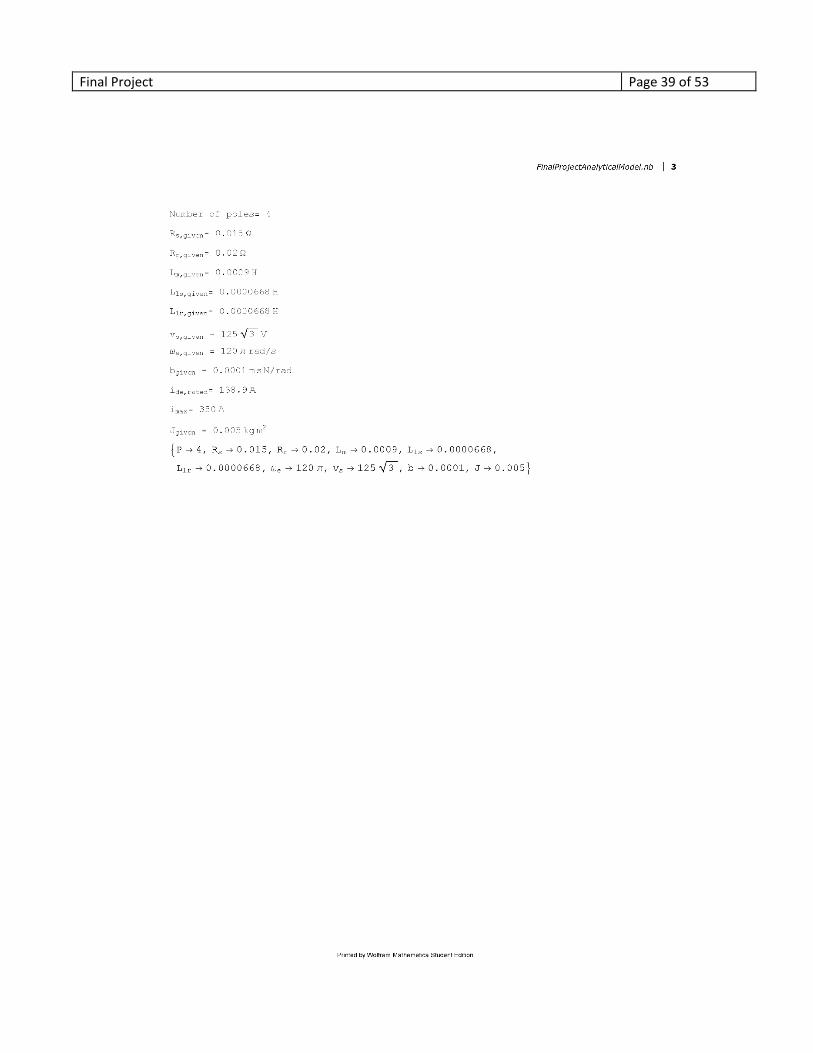
Introduction Tesla Motors, Inc. designs, builds, and sells electric vehicles [1]. The power trains of the Tesla cars use an induction motor to convert electrical energy in the battery to mechanical power at the wheels. Table 1 below shows the estimated motor parameters for the induction motor and Table 2 shows the rated motor values: Table 1 ‐ Summary of Induction Motor Parameters

4 0.015Ω 0.020 Ω 0.9mH

0.0668mH 0.0668mH

0.9668

0.9668

0.005 1.0 10

Table 2 ‐ Motor rated values

100 0.125Wb 138.9 375

350

The project scope will include the following items: 1) Simulate the TESLA induction machine using PLECS. Use notation consistent with the notation from the

class notes. 2) Simulate the current regulated induction machine with indirect field oriented control. Assume an ideal

inverter and perfectly estimated parameters. a. Implement a synchronous reference frame current regulator. b. Tune the q and d axis regulators for bandwidths of 1 kHz assuming that the parameter estimates

are accurate. c. Simulate a locked rotor step response for a rated torque command with d‐axis current held

constant at its rated value. d. Simulate a locked rotor 10 Hz, 100 Hz, and 1000 Hz sine wave response for a rated torque

command with d‐axis current held constant at its rated value. (A frequency response sweep is also acceptable).

3) Close a speed loop around the torque loop and demonstrate speed control of the motor. a. Tune the speed loop for a bandwidth of 50 Hz b. Simulate sine wave speed commands of 5 Hz and 50 Hz with a 10 rad/sec amplitude.

4) Connect the motor to a typical Tesla S gearbox and wheels and optimize for track conditions a. Optimize the system to achieve the best 0‐60 mph time. b. Optimize the system to achieve the best 0‐60‐0 mph time using regenerative braking. c. Optimize the system to achieve the best 0‐60‐0 mph time with the minimal use of power

(battery life).


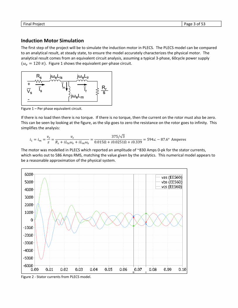
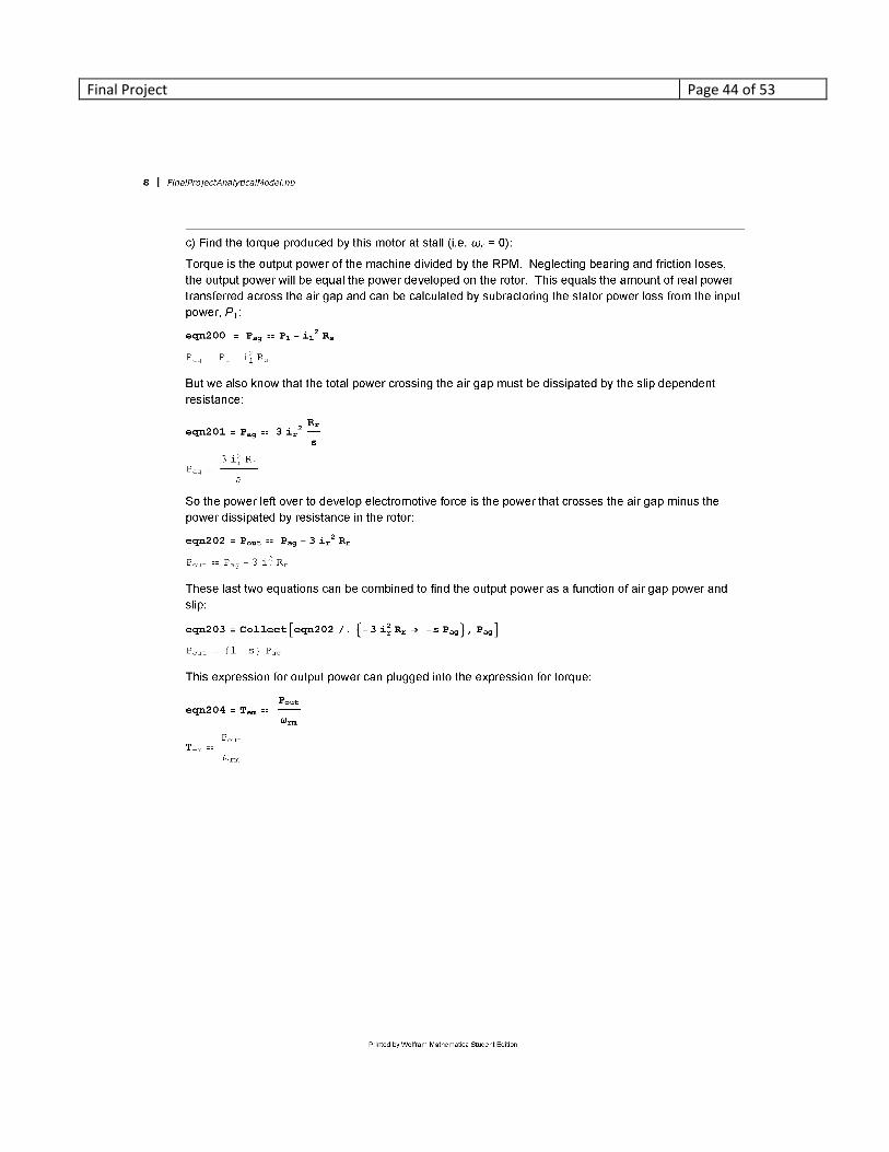
Induction Motor Simulation The first step of the project will be to simulate the induction motor in PLECS. The PLECS model can be compared to an analytical result, at steady state, to ensure the model accurately characterizes the physical motor. The analytical result comes from an equivalent circuit analysis, assuming a typical 3‐phase, 60cycle power supply

120 . Figure 1 shows the equivalent per‐phase circuit.

Figure 1 – Per phase equivalent circuit.

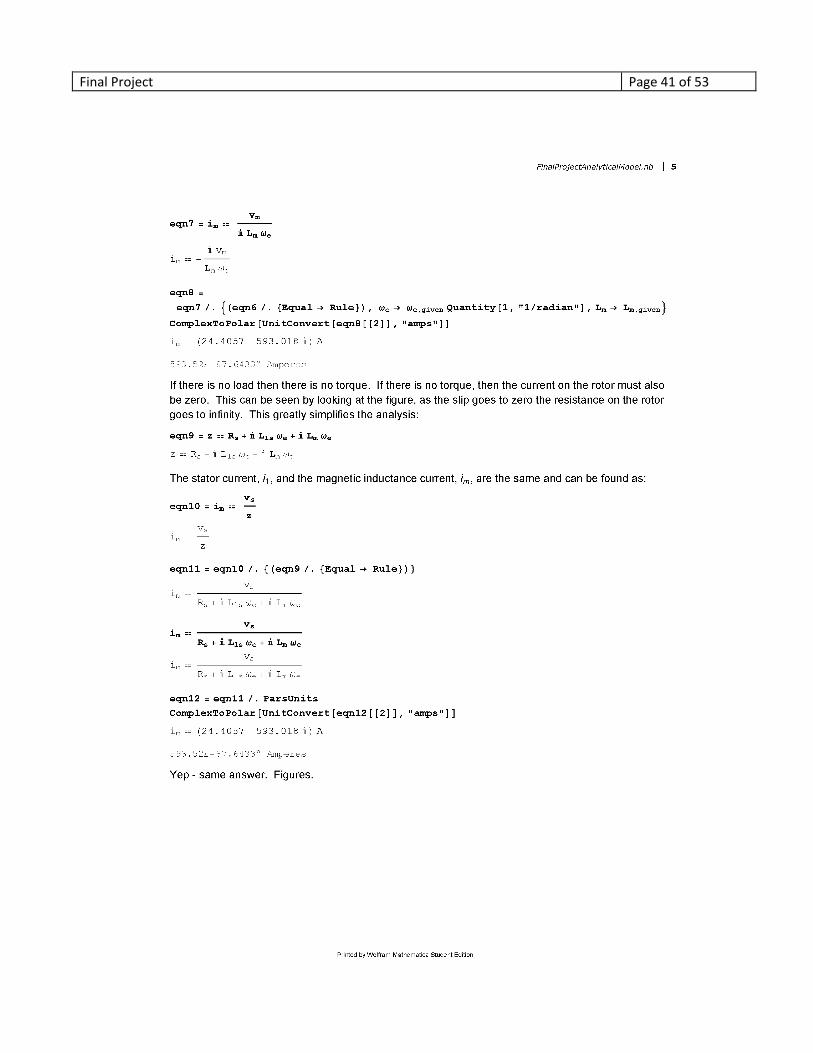
If there is no load then there is no torque. If there is no torque, then the current on the rotor must also be zero. This can be seen by looking at the figure, as the slip goes to zero the resistance on the rotor goes to infinity. This simplifies the analysis:

375/√3

0.015Ω 0.0251Ω 0.339594∠ 87.6°Amperes

The motor was modelled in PLECS which reported an amplitude of ~830 Amps 0‐pk for the stator currents, which works out to 586 Amps RMS, matching the value given by the analytics. This numerical model appears to be a reasonable approximation of the physical system.

Figure 2 ‐ Stator currents from PLECS model.


Current Regulated Induction Machine with Indirect FOC The modeling begins by tuning the current regulators to have a bandwidth of 1000 Hz. The full transient relationship for the stator current and voltages have cross‐coupling and back EMF components that make it difficult to design the current regulator. Figure 3 shows the synchronous frame current regulator in block diagram form.

Figure 3 ‐ Synchronous reference frame current regulator.

For the motor parameters of this problem and to achieve a bandwidth of 1000 hertz (Appendix A has the details), the gains for the proportional‐integral (PI) controller can be found as:

203Ω/

0.810Ω


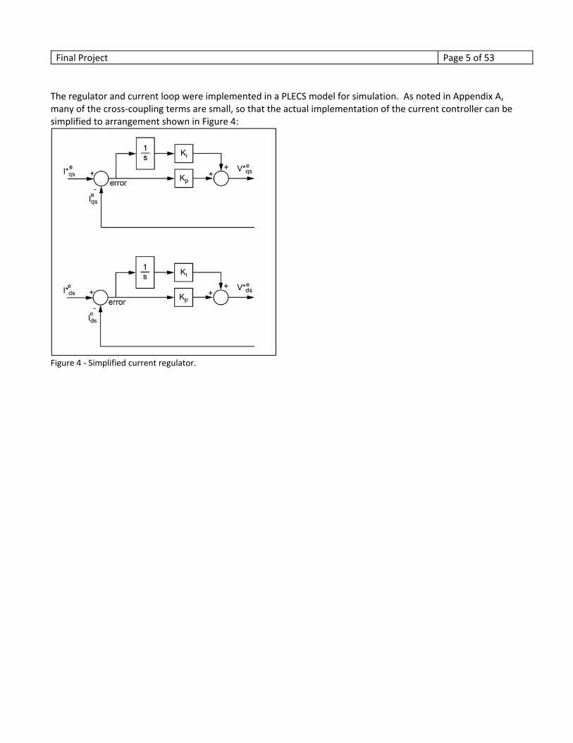
The regulator and current loop were implemented in a PLECS model for simulation. As noted in Appendix A, many of the cross‐coupling terms are small, so that the actual implementation of the current controller can be simplified to arrangement shown in Figure 4:

Figure 4 ‐ Simplified current regulator.


Without the cross‐coupling terms, there will be some effect on the current output, but it should be small. The current regulator can now be combined with the physical plant, as shown in the control diagram in Figure 5. The ‐axis regulator, ‐axis regulator, Park transform, Clarke transform, and the slip (frequency) calculator are all

explained in more detail in the appendices. Although there are additional transforms, this control loop can be reduced down to a current regulation problem much like that of a DC motor.

Figure 5 – Rotor flux field oriented induction machine control. Redrawn from [3, page 11].


Figure 4 shows command tracking for both the ‐axis and ‐axis currents. In response to the step function, the current settles out at the desired value in about 0.001 seconds, just about what is desired for a bandwidth of 1000 hertz. There are some cross‐coupling artifacts in both signals since there was no decoupling within the current regulator. The artifacts appear small and seem to be acceptable; however, if time allows it would be fun to add the decoupling and see if the artifacts disappear.

Figure 6 ‐ Current command tracking response to step function.


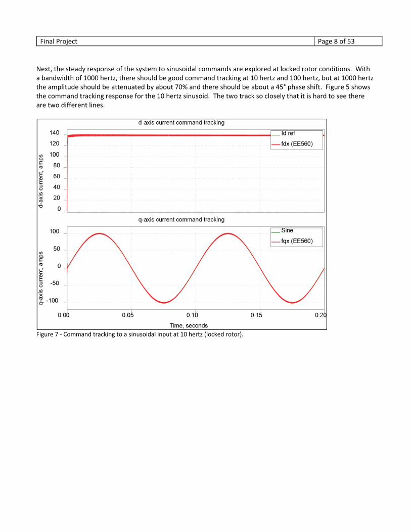
Next, the steady response of the system to sinusoidal commands are explored at locked rotor conditions. With a bandwidth of 1000 hertz, there should be good command tracking at 10 hertz and 100 hertz, but at 1000 hertz the amplitude should be attenuated by about 70% and there should be about a 45° phase shift. Figure 5 shows the command tracking response for the 10 hertz sinusoid. The two track so closely that it is hard to see there are two different lines.

Figure 7 ‐ Command tracking to a sinusoidal input at 10 hertz (locked rotor).


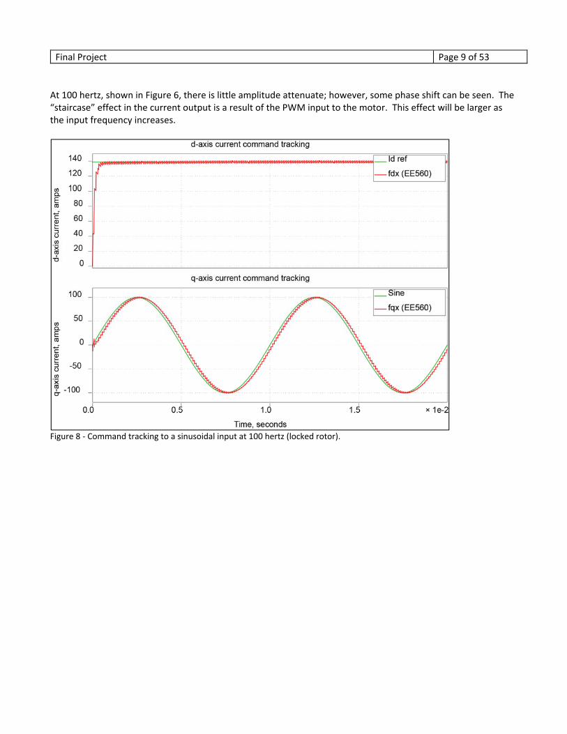
At 100 hertz, shown in Figure 6, there is little amplitude attenuate; however, some phase shift can be seen. The “staircase” effect in the current output is a result of the PWM input to the motor. This effect will be larger as the input frequency increases.



The response at 1000 hertz, shown in Figure 7, does have about the expected phase shift (45°), but the amplitude attenuation is not as much as expected. The stair case effect is much more pronounced and each switching cycle can clearly be seen. This suggests that the continuous‐time estimate is no longer a good approximation for the discrete‐time PWM. If the switching frequency is increased from 10kHz to 100kHz, there should be better agreement between the continuous‐time predication and the discrete‐time response.



Figure 8 shows the response at the higher switching frequency. The response is attenuated by about 70% and has the 45° degree phase shift. With the good agreement between the predicted response and the actual response it appears that the controller is working as expected, if the PWM switching frequency can be raised to 100 kHz. If the switching losses are too high at this frequency, then the bandwidth will have to be lowered to ensure the controller performs as desired.

Figure 10 ‐ Command tracking to a sinusoidal input at 1000 hertz and PWM switching frequency increased to 100 kHz (locked rotor).


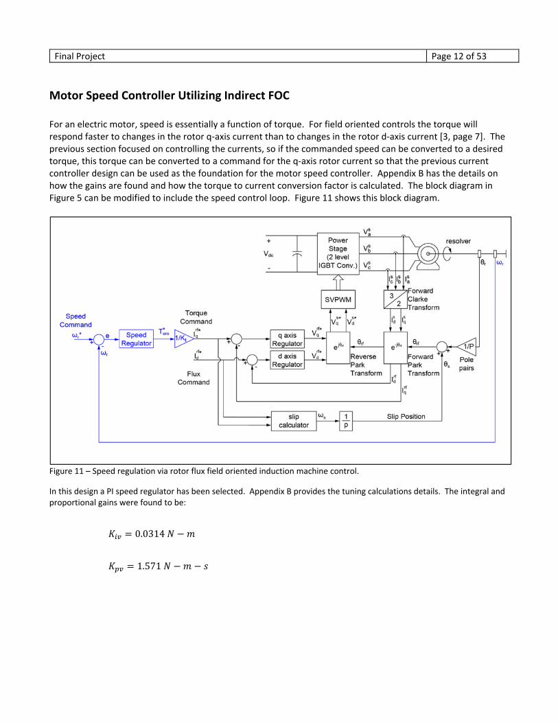
Motor Speed Controller Utilizing Indirect FOC For an electric motor, speed is essentially a function of torque. For field oriented controls the torque will respond faster to changes in the rotor q‐axis current than to changes in the rotor d‐axis current [3, page 7]. The previous section focused on controlling the currents, so if the commanded speed can be converted to a desired torque, this torque can be converted to a command for the q‐axis rotor current so that the previous current controller design can be used as the foundation for the motor speed controller. Appendix B has the details on how the gains are found and how the torque to current conversion factor is calculated. The block diagram in Figure 5 can be modified to include the speed control loop. Figure 11 shows this block diagram.

Figure 11 – Speed regulation via rotor flux field oriented induction machine control.

In this design a PI speed regulator has been selected. Appendix B provides the tuning calculations details. The integral and proportional gains were found to be:

0.0314

1.571


With these gains, validation of the tuner can begin. Starting with a command frequency of 100 RPM at 0.5 hertz, there should be good agreement between the commanded speed and measured speed, once the transients settle out. Figure 12 shows this data for the first 3 seconds of operation. There is very good agreement between the two values, once the transients settle out.

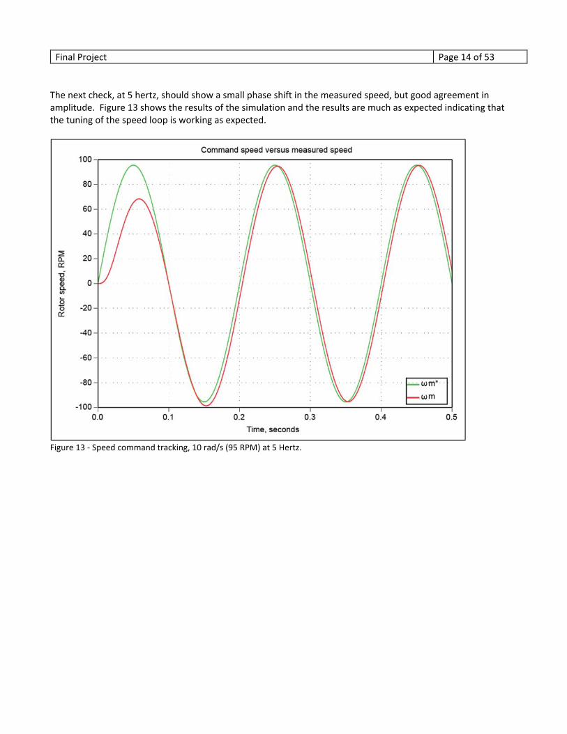
Figure 12 ‐ Speed command tracking, 10 rad/s (95 RPM) at 0.5 Hertz.


The next check, at 5 hertz, should show a small phase shift in the measured speed, but good agreement in amplitude. Figure 13 shows the results of the simulation and the results are much as expected indicating that the tuning of the speed loop is working as expected.

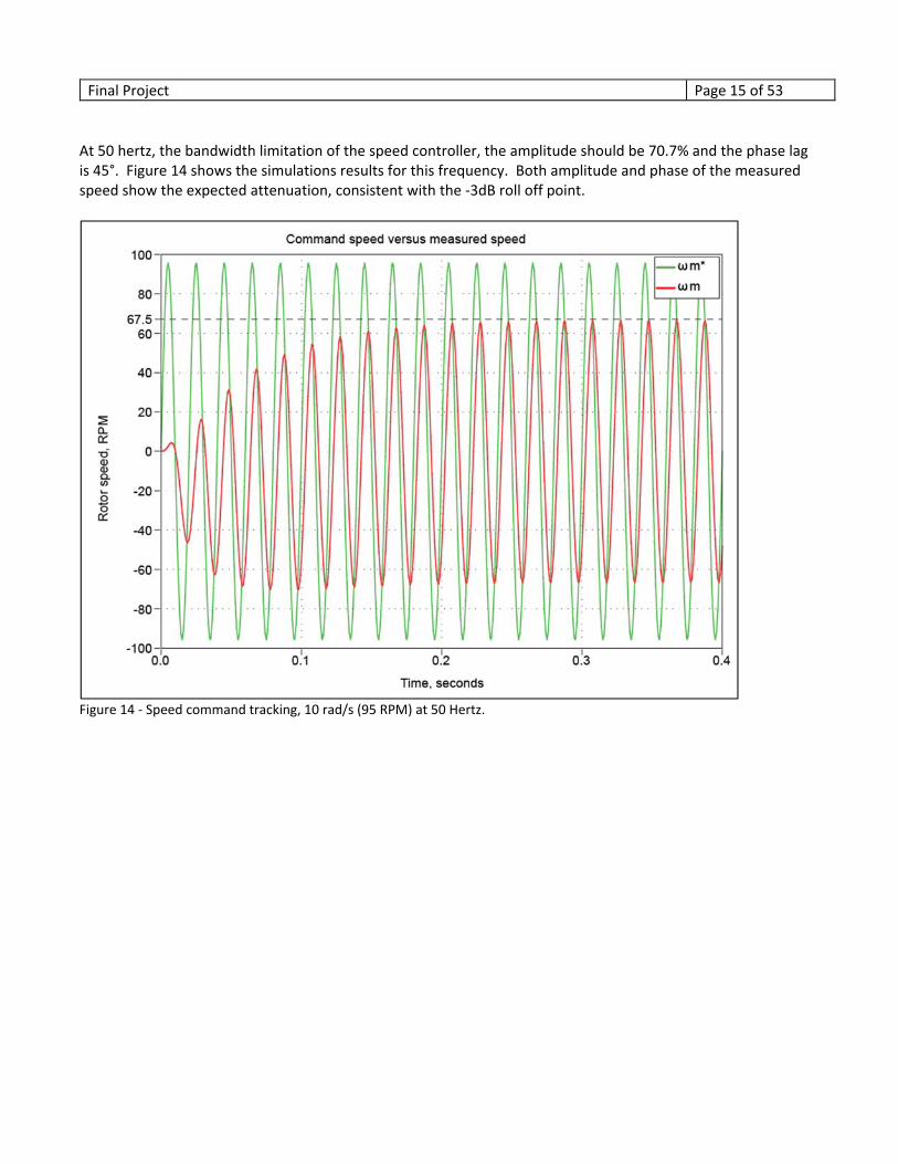
Figure 13 ‐ Speed command tracking, 10 rad/s (95 RPM) at 5 Hertz.


At 50 hertz, the bandwidth limitation of the speed controller, the amplitude should be 70.7% and the phase lag is 45°. Figure 14 shows the simulations results for this frequency. Both amplitude and phase of the measured speed show the expected attenuation, consistent with the ‐3dB roll off point.

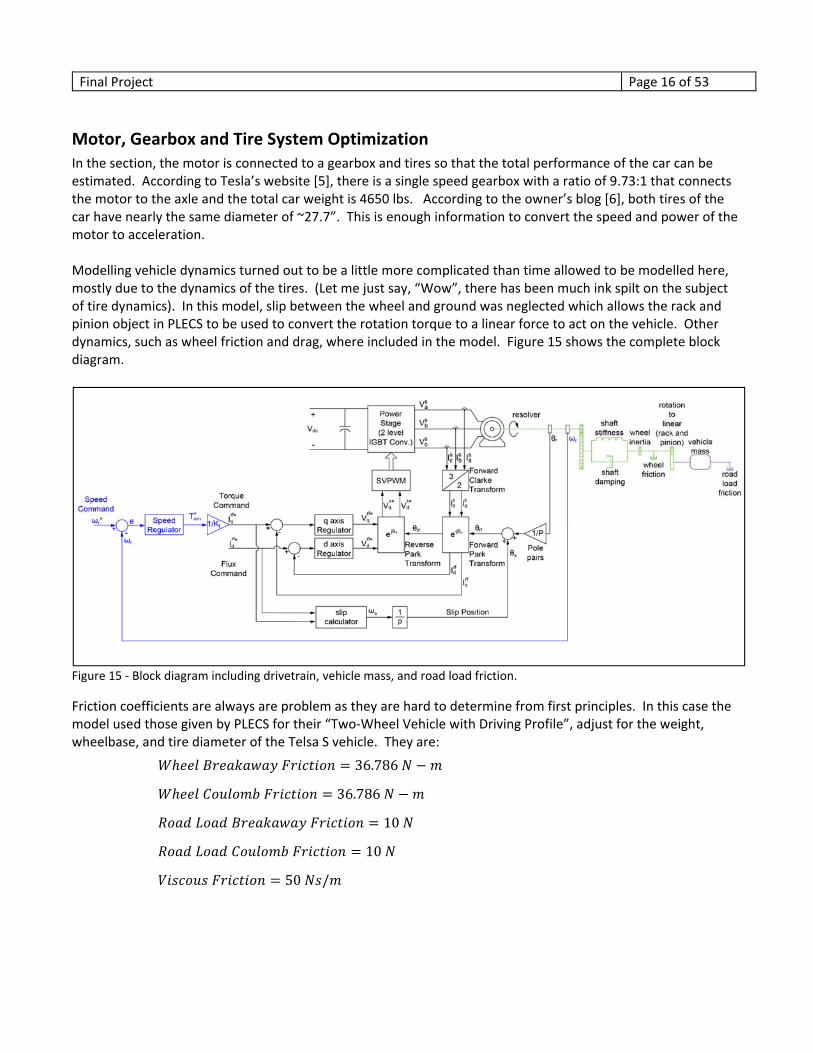
Figure 14 ‐ Speed command tracking, 10 rad/s (95 RPM) at 50 Hertz.


Motor, Gearbox and Tire System Optimization In the section, the motor is connected to a gearbox and tires so that the total performance of the car can be estimated. According to Tesla’s website [5], there is a single speed gearbox with a ratio of 9.73:1 that connects the motor to the axle and the total car weight is 4650 lbs. According to the owner’s blog [6], both tires of the car have nearly the same diameter of ~27.7”. This is enough information to convert the speed and power of the motor to acceleration. Modelling vehicle dynamics turned out to be a little more complicated than time allowed to be modelled here, mostly due to the dynamics of the tires. (Let me just say, “Wow”, there has been much ink spilt on the subject of tire dynamics). In this model, slip between the wheel and ground was neglected which allows the rack and pinion object in PLECS to be used to convert the rotation torque to a linear force to act on the vehicle. Other dynamics, such as wheel friction and drag, where included in the model. Figure 15 shows the complete block diagram.

Figure 15 ‐ Block diagram including drivetrain, vehicle mass, and road load friction.

Friction coefficients are always are problem as they are hard to determine from first principles. In this case the model used those given by PLECS for their “Two‐Wheel Vehicle with Driving Profile”, adjust for the weight, wheelbase, and tire diameter of the Telsa S vehicle. They are:

36.786

36.786

10

10

50 /


Preliminary Results

Given the somewhat primitive implementation and guesses about the friction, how did the model perform? Figure 16 shows the model response to step in command speed to 100 rad/s (4774 RPM). The model reached 0‐60 at 3.8 seconds, which is faster than the actual Tesla S car.

Figure 16 – Vehicle speed versus time, 0‐60 MPH.

The trend plot for the motor indicated that the motor reached 147 rad/s (1408 RPM), which is too low. After working through the model, two conversion errors were found that resulted in this curve. At 60 MPH, with a 9.73 gear ratio and 27.7” tires, the motor should be turning at about 7,084 RPM. This the point at which the owner’s blog [6] say field weakening begins in the Tesla.


Model Tuning

Figure 17 shows the resulting vehicle speed and motor speed plot after correcting the conversion errors. The Tesla Motors club blog [6] suggests that the Tesla S should be able to do this in something between 4.2 and 5.5 seconds, depending on the model. The PLECS model reaches 60 mph in 4.6 seconds, right about in the middle of the range. This time the step command was to 8,000 RPM.

Figure 17 ‐ Vehicle speed and motor speed versus time, 0‐60 MPH.


Digging a little bit more into the data, however, showed that the motor controller was not running well. As shown in Figure 18, current command tracking was awful. In addition, the controller was commanding much more that the rated current.

Figure 18 ‐ Current command tracking, 0‐60 (step input).


The current command tracking could be improved somewhat by using a ramp input instead of step input. Figure 19 shows the current command tracking for this case. There is much better agreement between the command and actual current; however it is still above the rated current.

Figure 19 ‐ Current command tracking, 0‐60 (ramp input).


As would be expected, adding the saturation limits to the current made the car run slower. With these limits no combination of inputs were found that would allow the car to run 0‐60 MPH in less than 6 seconds. Figure 20 shows the results for the best run.

Figure 20 ‐ Vehicle speed and motor speed versus time, 0‐60 MPH with ramp input and saturation limits on the current.


Summary

Getting the model to 60 MPH turned out to be more difficult than expected. It seems that there is quite a bit of tuning and adjustment that will be needed to be added to the model. Despite the addition work needed, it does seem like it would be possible to build a complete vehicle model for the Tesla drive train and simulate it in PLECS.

Conclusion In this project both the current loop and speed loop were successfully tuned to the specifications of the project. In addition, the model was revised to include a representation of the mechanical components of the Tesla S drive train. Unfortunately, this model was not able to match the actual car performance closely. Even with this difficulty, the opportunity to tune and apply field orientated control in vehicle was fun. It really showcases how important and pervasive these types of control systems have become in our lives.


Appendix A – Current Regulator Block Diagram Derivation

Transient tuning

Form reference [2] the stator voltage can be related to the stator current and flux, in the Laplace domain, as:

̅ ω ̅ ̅ Eq. A.1

Where

1

τ

Equation A.1 can be separated into real and imaginary parts:

Eq. A.2a

Eq. A.2b

If the rotor flux is positioned so that it is aligned with the d‐axis (no q‐axis rotor flux), then the equations simplify further:

Eq. A.3a

Eq. A.3b


These equations can be drawing in block diagram form as:

Figure A1 – Block diagram relating current to voltage and rotor flux.

This is a little complicated for tuning so some assumptions will be made: ‐ Lock the rotor to eliminate terms related to rotor speed. ‐ The cross coupling factor, , is less than 1, the stator inductance, , is much less than 1 so that

multiplying these factors times electrical frequency and current does not result in a large number. So the cross coupling terms can be neglected.

‐ The rotor resistance is close to zero and the direct rotor flux is close to unity (at steady state conditions and ~10 , ~10 ) so those terms will be neglected.


That takes care of the coupling so that each current loop can be tuned independently. It also simplifies the analysis of the simplified closed‐loop system, shown in Figure A2:

Figure A2 ‐ Simplified current control loop.

This is essentially the same structure as the DC motor current control loop in which it was shown that the gains, at locked rotor conditions, can be calculated as [3, page 17]:

2 Ω/s

2 Ω

For the motor parameters of this problem, the gains work out to:

2

1

1000 0.0323 Ω

1203 Ω/

2

1

1000 0.133414

1

0.0009668 Ω sec

10.810 Ω

Steady state tuning

Equations A.3b can be simplified some by considering the steady state case. At steady state conditions, the ‐axis flux is proportional to ‐axis current [4, page 2], [3, pages 2‐3]:

This, along with the expression for , can be substituted into Equation A.3b to find:

Eq. A.3b

This changes the integral gain, , as:

, 2 Ω

s

2

1

1000 0.015 Ω

194.2 Ω/


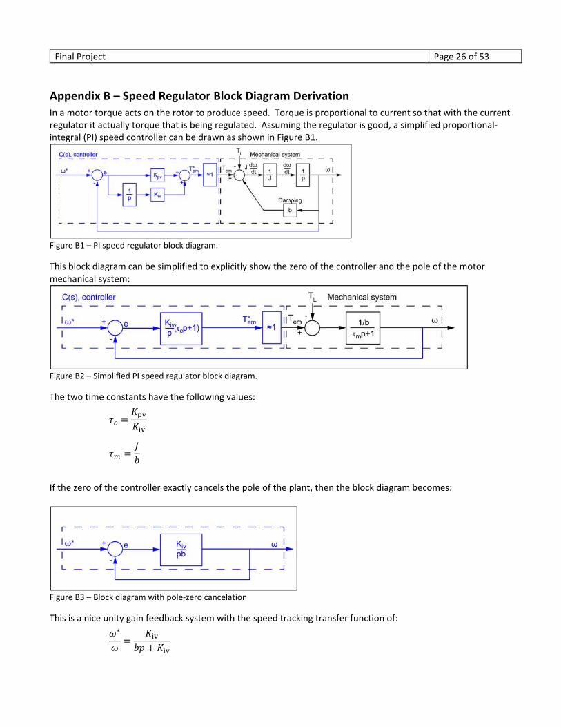
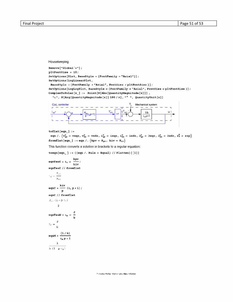
Appendix B – Speed Regulator Block Diagram Derivation In a motor torque acts on the rotor to produce speed. Torque is proportional to current so that with the current regulator it actually torque that is being regulated. Assuming the regulator is good, a simplified proportional‐integral (PI) speed controller can be drawn as shown in Figure B1.

Figure B1 – PI speed regulator block diagram.

This block diagram can be simplified to explicitly show the zero of the controller and the pole of the motor mechanical system:

Figure B2 – Simplified PI speed regulator block diagram.

The two time constants have the following values:

If the zero of the controller exactly cancels the pole of the plant, then the block diagram becomes:

Figure B3 – Block diagram with pole‐zero cancelation

This is a nice unity gain feedback system with the speed tracking transfer function of:

∗


The magnitude of the transfer function should be ‐3dB at the desired frequency response (where ):

∗

⇒

1

√2⇒ 2

From the definition of the time constants and the desire to make them equal for pole‐zero cancellation, the value for the proportional gain can be found as:

⇒ 2 2

Using the values for this motor

2

1

50 0.0001 N m

/0.0314

2

1

50 0.005 kg m

1

100

0.005 N m sec

11.571

The controller provides the commanded torque value and this must be converted to current. One way to express the torque for an induction motor is to write it as a function of the cross‐product of the rotor and stator flux:

3

2 2Im ̅ ̅

In field oriented control, the rotor flux is aligned with the d‐axis so that the quadrature component of the rotor flux, , will be zero [4, page 12]:

3

2 2

This can be re‐arranged to find quadrature current as a function of torque:

4

3 Eq. B‐1

If the flux command (d‐axis current) is constant, then Equation B‐1 can be written as:

1

Eq. B‐2

Where:

3

4

In this form it can be seen that the expression for torque is similar to that of a DC motor.


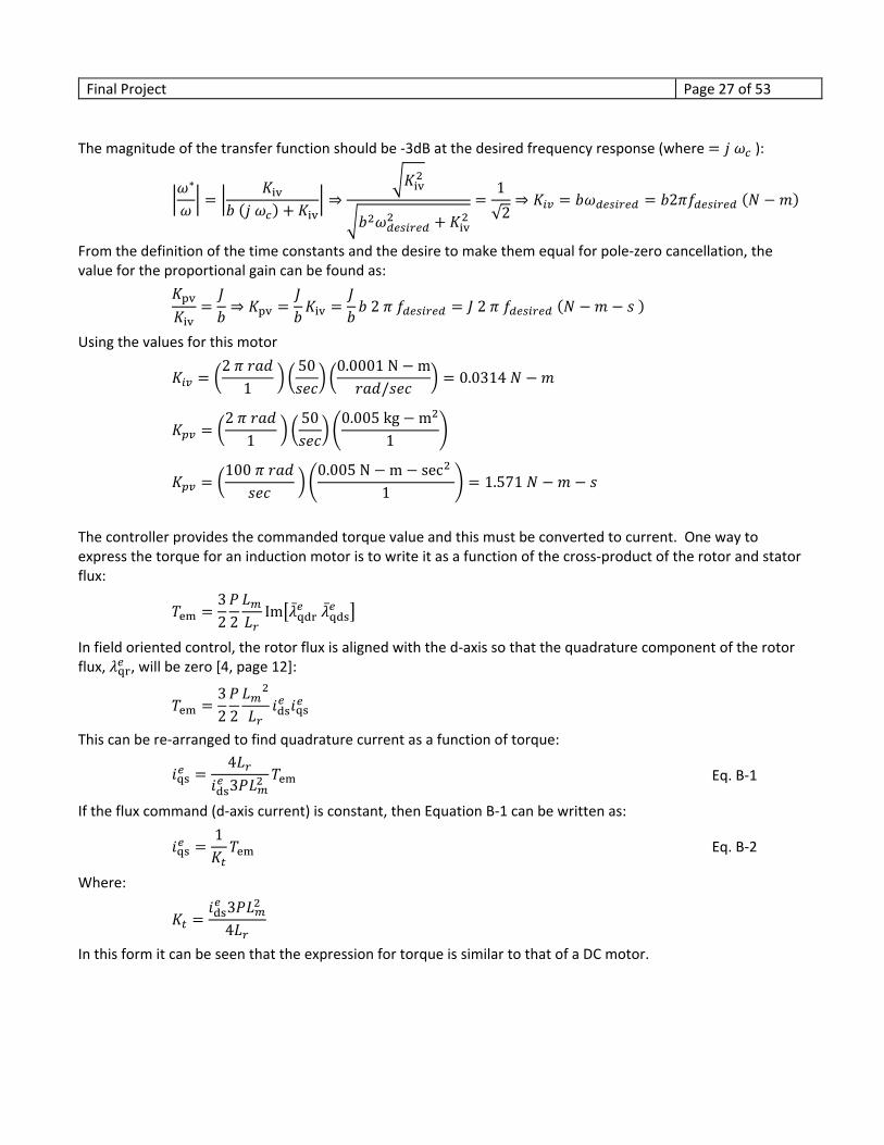
Appendix C – Slip Calculations Since the rotor of an induction motor turns at a frequency slightly less then electrical frequency, the control laws must include a compensator to correct the mechanical rotor angle to the electrical angle. In the rotor flux, or synchronous, reference frame the block diagram can be drawn as:

Figure C1 ‐ Slip frequency calculation. (redrawn from [3, page 8]).

This figure can be simplified a bit though block diagram reduction and drawn as:

Figure C2 – Slip frequency calculation (simplified).


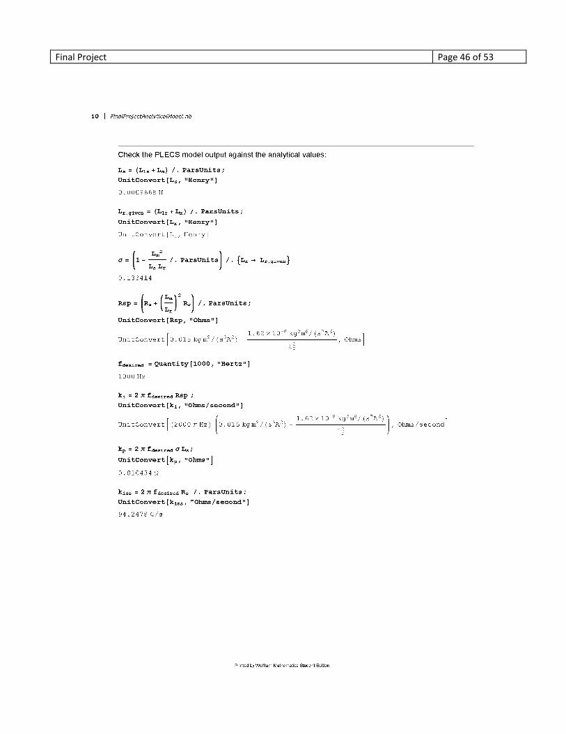
In Figure C2, the two mutual inductances cancel out and the / term is equal to [3, page 6] so that the calculator can be further simplified as shown in Figure C3. It was this form that was implemented within PLECS.

Figure C3 ‐ Slip frequency calculation, as implemented in PLECS.


Appendix D – PLECS Model

Figure D1 ‐ Overall PLECS Model.

Figure D2 – Speed controller.


Figure D3 ‐ Motor Controller.

Figure D4 ‐ Current Controller.


Figure D5 ‐ Current regulator.

Figure D6 ‐ Motor overall view.


Figure D7 ‐ Motor currents calculation.


Figure D8 ‐ Motor flux linkage calculation.

Figure D9 ‐ Tesla drive train model.


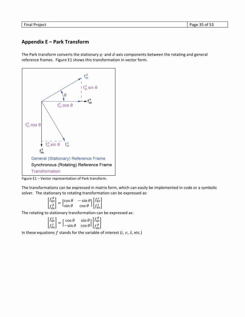
Appendix E – Park Transform The Park transform converts the stationary ‐ and ‐axis components between the rotating and general reference frames. Figure E1 shows this transformation in vector form.

Figure E1 – Vector representation of Park transform.

The transformations can be expressed in matrix form, which can easily be implemented in code or a symbolic solver. The stationary to rotating transformation can be expressed as:

cos sinsin cos

The rotating to stationary transformation can be expressed as:

cos sinsin cos

In these equations stands for the variable of interest ( , , , etc.)


Appendix F – Clarke Transform The Clarke transform converts the 3 vectors into 2 orthogonal vectors. Figure F1 shows the transform in vector form. The 3‐phase components are projected onto the quadrature ‐ axis.

Figure 21 – Vector representation of the Clarke transform.

Much like the Park transform, the Clarke transform can be represented as matrix operations. The transformation from 3‐Phase to ‐ (forward transformation) can be written as:

2

3

11

2

1

2

0√3

2

√3

21

2

1

2

1

2

The rotating to stationary transformation can be expressed as:

1 0 1

1

2

√3

21

1

2

√3

21

In these equations stands for the variable of interest ( , , , etc.)


Appendix G ‐ Mathematica Code

















References

1. "Tesla Motors." Wikipedia. Wikimedia Foundation, 25 Nov. 2014. Web. 25 Nov. 2014.

2. Nagel, N. J. "EE 560 – Electric Machines and Drives." Lecture 8. University of Washington, 24

Nov. 2014.

3. Nagel, N. J. "EE 560 – Electric Machines and Drives." Lecture 7. University of Washington, 17

Nov. 2014.

4. Nagel, N. J. "EE 560 – Electric Machines and Drives." Lecture 9. University of Washington, 1 Dec.

2014.

5. Tesla Motors Inc. "Specs." Model S. N.p., n.d. Web. 06 Dec. 2014.

6. "Thread: The Real Top Speed of the Model S." Tesla Motors Club Enthusiasts Owners Forum RSS.

N.p., n.d. Web. 06 Dec. 2014. <http://www.teslamotorsclub.com/showthread.php/17256‐The‐

real‐top‐speed‐of‐the‐Model‐S/page4?p=354969&viewfull=1#post354969>.

Date post:	06-Jul-2018
Category:	Documents
Upload:	buingoc
View:	215 times
Download:	0 times

Contents 3 Machine and 16 -...

Documents