Contents Contents i List of Tables ii List of Figures iii 5 Noninteracting Quantum Systems 1 5.1 References .............................................. 1 5.2 Statistical Mechanics of Noninteracting Quantum Systems .................. 2 5.2.1 Bose and Fermi systems in the grand canonical ensemble .............. 2 5.2.2 Quantum statistics and the Maxwell-Boltzmann limit ................ 3 5.2.3 Single particle density of states ............................. 5 5.3 Quantum Ideal Gases : Low Density Expansions ........................ 6 5.3.1 Expansion in powers of the fugacity .......................... 6 5.3.2 Virial expansion of the equation of state ........................ 7 5.3.3 Ballistic dispersion .................................... 9 5.4 Entropy and Counting States ................................... 9 5.5 Photon Statistics .......................................... 11 5.5.1 Thermodynamics of the photon gas ........................... 11 5.5.2 Classical arguments for the photon gas ......................... 13 5.5.3 Surface temperature of the earth ............................. 14 5.5.4 Distribution of blackbody radiation ........................... 15 i
5.17 Mean field phase diagram of the Hubbard model, including paramagnetic (P), ferromag-netic (F), and antiferromagnetic (A) phases. Left panel: results using a semicircular den-sity of states function of half-bandwidth W . Right panel: results using a two-dimensionalsquare lattice density of states with nearest neighbor hopping t, from J. E. Hirsch, Phys.Rev. B 31, 4403 (1985). The phase boundary between F and A phases is first order. . . . . . 60
– F. Reif, Fundamentals of Statistical and Thermal Physics (McGraw-Hill, 1987)This has been perhaps the most popular undergraduate text since it first appeared in 1967, andwith good reason.
– A. H. Carter, Classical and Statistical Thermodynamics(Benjamin Cummings, 2000)A very relaxed treatment appropriate for undergraduate physics majors.
– D. V. Schroeder, An Introduction to Thermal Physics (Addison-Wesley, 2000)This is the best undergraduate thermodynamics book I’ve come across, but only 40% of the booktreats statistical mechanics.
– C. Kittel, Elementary Statistical Physics (Dover, 2004)Remarkably crisp, though dated, this text is organized as a series of brief discussions of key con-cepts and examples. Published by Dover, so you can’t beat the price.
– R. K. Pathria, Statistical Mechanics (2nd edition, Butterworth-Heinemann, 1996)This popular graduate level text contains many detailed derivations which are helpful for thestudent.
– M. Plischke and B. Bergersen, Equilibrium Statistical Physics (3rd edition, World Scientific, 2006)An excellent graduate level text. Less insightful than Kardar but still a good modern treatment ofthe subject. Good discussion of mean field theory.
– E. M. Lifshitz and L. P. Pitaevskii, Statistical Physics (part I, 3rd edition, Pergamon, 1980)This is volume 5 in the famous Landau and Lifshitz Course of Theoretical Physics . Though dated,it still contains a wealth of information and physical insight.
1
2 CHAPTER 5. NONINTERACTING QUANTUM SYSTEMS
5.2 Statistical Mechanics of Noninteracting Quantum Systems
5.2.1 Bose and Fermi systems in the grand canonical ensemble
A noninteracting many-particle quantum Hamiltonian may be written as1
H =∑α
εα nα , (5.1)
where nα is the number of particles in the quantum state α with energy εα. This form is called thesecond quantized representation of the Hamiltonian. The number eigenbasis is therefore also an energyeigenbasis. Any eigenstate of H may be labeled by the integer eigenvalues of the nα number operators,and written as
∣∣n1 , n2 , . . .⟩
. We then have
nα∣∣~n ⟩ = nα
∣∣~n ⟩ (5.2)
andH∣∣~n ⟩ =
∑α
nα εα∣∣~n ⟩ . (5.3)
The eigenvalues nα take on different possible values depending on whether the constituent particles arebosons or fermions, viz.
bosons : nα ∈
0 , 1 , 2 , 3 , . . .
fermions : nα ∈
0 , 1.
(5.4)
In other words, for bosons, the occupation numbers are nonnegative integers. For fermions, the occupa-tion numbers are either 0 or 1 due to the Pauli principle, which says that at most one fermion can occupyany single particle quantum state. There is no Pauli principle for bosons.
The N -particle partition function ZN is then
ZN =∑nα
e−β∑α nαεα δN ,
∑α nα
, (5.5)
where the sum is over all allowed values of the set nα, which depends on the statistics of the particles.Bosons satisfy Bose-Einstein (BE) statistics, in which nα ∈ 0 , 1 , 2 , . . .. Fermions satisfy Fermi-Dirac(FD) statistics, in which nα ∈ 0 , 1.
The OCE partition sum is difficult to perform, owing to the constraint∑
α nα = N on the total numberof particles. This constraint is relaxed in the GCE, where
Ξ =∑N
eβµN ZN
=∑nα
e−β∑α nαεα eβµ
∑α nα
=∏α
(∑nα
e−β(εα−µ)nα
).
(5.6)
1For a review of the formalism of second quantization, see the appendix in §5.9.
5.2. STATISTICAL MECHANICS OF NONINTERACTING QUANTUM SYSTEMS 3
Note that the grand partition function Ξ takes the form of a product over contributions from the indi-vidual single particle states.
We now perform the single particle sums:
∞∑n=0
e−β(ε−µ)n =1
1− e−β(ε−µ)(bosons) (5.7)
1∑n=0
e−β(ε−µ)n = 1 + e−β(ε−µ) (fermions) . (5.8)
Therefore we have
ΞBE =∏α
1
1− e−(εα−µ)/kBT
ΩBE = kBT∑α
ln(
1− e−(εα−µ)/kBT) (5.9)
and
ΞFD =∏α
(1 + e−(εα−µ)/kBT
)ΩFD = −kBT
∑α
ln(
1 + e−(εα−µ)/kBT).
(5.10)
We can combine these expressions into one, writing
Ω(T, V, µ) = ±kBT∑α
ln(
1∓ e−(εα−µ)/kBT), (5.11)
where we take the upper sign for Bose-Einstein statistics and the lower sign for Fermi-Dirac statistics.Note that the average occupancy of single particle state α is
〈nα〉 =∂Ω
∂εα=
1
e(εα−µ)/kBT ∓ 1, (5.12)
and the total particle number is then
N(T, V, µ) =∑α
1
e(εα−µ)/kBT ∓ 1. (5.13)
We will henceforth write nα(µ, T ) = 〈nα〉 for the thermodynamic average of this occupancy.
5.2.2 Quantum statistics and the Maxwell-Boltzmann limit
Consider a system composed of N noninteracting particles. The Hamiltonian is
H =
N∑j=1
hj . (5.14)
4 CHAPTER 5. NONINTERACTING QUANTUM SYSTEMS
The single particle Hamiltonian h has eigenstates |α〉 with corresponding energy eigenvalues εα. Whatis the partition function? Is it
Z?=∑α1
· · ·∑αN
e−β(εα1
+ εα2
+ ... + εαN
)= ζN , (5.15)
where ζ is the single particle partition function,
ζ =∑α
e−βεα . (5.16)
For systems where the individual particles are distinguishable, such as spins on a lattice which have fixedpositions, this is indeed correct. But for particles free to move in a gas, this equation is wrong. Thereason is that for indistinguishable particles the many particle quantum mechanical states are specified bya collection of occupation numbers nα, which tell us how many particles are in the single-particle state|α 〉. The energy is
E =∑α
nα εα (5.17)
and the total number of particles isN =
∑α
nα . (5.18)
That is, each collection of occupation numbers nα labels a unique many particle state∣∣ nα ⟩. In the
product ζN , the collection nα occurs many times. We have therefore overcounted the contribution toZN due to this state. By what factor have we overcounted? It is easy to see that the overcounting factoris
degree of overcounting =N !∏α nα!
,
which is the number of ways we can rearrange the labels αj to arrive at the same collection nα. Thisfollows from the multinomial theorem,(
K∑α=1
xα
)N=∑n1
∑n2
· · ·∑nK
N !
n1!n2! · · ·nK !xn11 x
n22 · · ·x
nKK δN,n1 + ...+nK
. (5.19)
Thus, the correct expression for ZN is
ZN =∑nα
e−β∑α nαεα δN,
∑α nα
=∑α1
∑α2
· · ·∑αN
(∏α nα!
N !
)e−β(εα1
+ εα2+ ... + εα
N).
(5.20)
In the high temperature limit, almost all the nα are either 0 or 1, hence
ZN ≈ζN
N !. (5.21)
5.2. STATISTICAL MECHANICS OF NONINTERACTING QUANTUM SYSTEMS 5
This is the classical Maxwell-Boltzmann limit of quantum statistical mechanics. We now see the origin ofthe 1/N ! term which is so important in the thermodynamics of entropy of mixing.
Finally, starting with the expressions for the grand partition function for Bose-Einstein or Fermi-Diracparticles, and working in the low density limit where nα(µ, T ) 1 , we have εα − µ kBT , andconsequently
ΩBE/FD
= ±kBT∑α
ln(
1∓ e−(εα−µ)/kBT)
−→ −kBT∑α
e−(εα−µ)/kBT ≡ ΩMB .(5.22)
This is the Maxwell-Boltzmann limit of quantum statistical mechanics. The occupation number averagein the Maxwell-Boltzmann limit is then
〈nα〉 = e−(εα−µ)/kBT . (5.23)
5.2.3 Single particle density of states
The single particle density of states per unit volume g(ε) is defined as
g(ε) =1
V
∑α
δ(ε− εα) . (5.24)
We can then write
Ω(T, V, µ) = ±V kBT
∞∫−∞
dε g(ε) ln(
1∓ e−(ε−µ)/kBT). (5.25)
For particles with a dispersion ε(k), with p = ~k, we have
g(ε) = g
∫ddk
(2π)dδ(ε− ε(k)
)=
gΩd(2π)d
kd−1
dε/dk.
(5.26)
where g = 2S+1 is the spin degeneracy, and where we assume that ε(k) is both isotropic and a mono-tonically increasing function of k. Thus, we have
g(ε) =gΩd(2π)d
kd−1
dε/dk=
gπdkdε d = 1
g2π k
dkdε d = 2
g2π2 k
2 dkdε d = 3 .
(5.27)
In order to obtain g(ε) as a function of the energy ε one must invert the dispersion relation ε = ε(k) toobtain k = k(ε).
6 CHAPTER 5. NONINTERACTING QUANTUM SYSTEMS
Note that we can equivalently write
g(ε) dε = gddk
(2π)d=
gΩd(2π)d
kd−1 dk (5.28)
to derive g(ε).
For a spin-S particle with ballistic dispersion ε(k) = ~2k2/2m, we have
g(ε) =2S+1
Γ(d/2)
(m
2π~2
)d/2εd2−1 Θ(ε) , (5.29)
where Θ(ε) is the step function, which takes the value 0 for ε < 0 and 1 for ε ≥ 0. The appearanceof Θ(ε) simply says that all the single particle energy eigenvalues are nonnegative. Note that we areassuming a box of volume V but we are ignoring the quantization of kinetic energy, and assuming thatthe difference between successive quantized single particle energy eigenvalues is negligible so that g(ε)can be replaced by the average in the above expression. Note that
n(ε, T, µ) =1
e(ε−µ)/kBT ∓ 1. (5.30)
This result holds true independent of the form of g(ε). The average total number of particles is then
N(T, V, µ) = V
∞∫−∞
dε g(ε)1
e(ε−µ)/kBT ∓ 1, (5.31)
which does depend on g(ε).
5.3 Quantum Ideal Gases : Low Density Expansions
5.3.1 Expansion in powers of the fugacity
From eqn. 5.31, we have that the number density n = N/V is
n(T, z) =
∞∫−∞
dεg(ε)
z−1 eε/kBT ∓ 1
=∞∑j=1
(±1)j−1Cj(T ) zj ,
(5.32)
where z = exp(µ/kBT ) is the fugacity and
Cj(T ) =
∞∫−∞
dε g(ε) e−jε/kBT . (5.33)
5.3. QUANTUM IDEAL GASES : LOW DENSITY EXPANSIONS 7
From Ω = −pV and our expression above for Ω(T, V, µ), we have
p(T, z) = ∓ kBT
∞∫−∞
dε g(ε) ln(
1∓ z e−ε/kBT)
= kBT
∞∑j=1
(±1)j−1 j−1Cj(T ) zj .
(5.34)
5.3.2 Virial expansion of the equation of state
Eqns. 5.32 and 5.34 express n(T, z) and p(T, z) as power series in the fugacity z, with T -dependentcoefficients. In principal, we can eliminate z using eqn. 5.32, writing z = z(T, n) as a power series inthe number density n, and substitute this into eqn. 5.34 to obtain an equation of state p = p(T, n) of theform
p(T, n) = nkBT(
1 +B2(T )n+B3(T )n2 + . . .). (5.35)
Note that the low density limit n→ 0 yields the ideal gas law independent of the density of states g(ε).This follows from expanding n(T, z) and p(T, z) to lowest order in z, yielding n = C1 z + O(z2) andp = kBT C1 z + O(z2). Dividing the second of these equations by the first yields p = nkBT + O(n2),which is the ideal gas law. Note that z = n/C1 +O(n2) can formally be written as a power series in n.
Unfortunately, there is no general analytic expression for the virial coefficients Bj(T ) in terms of theexpansion coefficients nj(T ). The only way is to grind things out order by order in our expansions.Let’s roll up our sleeves and see how this is done. We start by formally writing z(T, n) as a power seriesin the density n with T -dependent coefficients Aj(T ):
z = A1 n+A2 n2 +A3 n
3 + . . . . (5.36)
We then insert this into the series for n(T, z):
n = C1 z ± C2 z2 + C3z
3 + . . .
= C1
(A1 n+A2 n
2 +A3 n3 + . . .
)± C2
(A1 n+A2 n
2 +A3 n3 + . . .
)2+ C3
(A1 n+A2 n
2 +A3 n3 + . . .
)3+ . . . .
(5.37)
Let’s expand the RHS to order n3. Collecting terms, we have
n = C1A1 n+(C1A2 ± C2A
21
)n2 +
(C1A3 ± 2C2A1A2 + C3A
31
)n3 + . . . . (5.38)
In order for this equation to be true we require that the coefficient of n on the RHS be unity, and that thecoefficients of nj for all j > 1 must vanish. Thus,
C1A1 = 1
C1A2 ± C2A21 = 0
C1A3 ± 2C2A1A2 + C3A31 = 0 .
(5.39)
8 CHAPTER 5. NONINTERACTING QUANTUM SYSTEMS
The first of these yields A1:
A1 =1
C1
. (5.40)
We now insert this into the second equation to obtain A2:
A2 = ∓C2
C31
. (5.41)
Next, insert the expressions for A1 and A2 into the third equation to obtain A3:
A3 =2C2
2
C51
− C3
C41
. (5.42)
This procedure rapidly gets tedious!
And we’re only half way done. We still must express p in terms of n:
p
kBT= C1
(A1 n+A2 n
2 +A3 n3 + . . .
)± 1
2C2
(A1 n+A2 n
2 +A3 n3 + . . .
)2+ 1
3C3
(A1 n+A2 n
2 +A3 n3 + . . .
)3+ . . .
= C1A1 n+(C1A2 ± 1
2C2A21
)n2 +
(C1A3 ± C2A1A2 + 1
3 C3A31
)n3 + . . .
= n+B2 n2 +B3 n
3 + . . .
(5.43)
We can now write
B2 = C1A2 ± 12C2A
21 = ∓ C2
2C21
B3 = C1A3 ± C2A1A2 + 13 C3A
31 =
C22
C41
− 2C3
3C31
.
(5.44)
It is easy to derive the general result that BFj = (−1)j−1BB
j , where the superscripts denote Fermi (F) orBose (B) statistics.
We remark that the equation of state for classical (and quantum) interacting systems also can be expandedin terms of virial coefficients. Consider, for example, the van der Waals equation of state,(
p+aN2
V 2
)(V −Nb) = NkBT . (5.45)
This may be recast as
p =nkBT
1− bn− an2
= nkBT +(b kBT − a
)n2 + kBT b
2n3 + kBT b3n4 + . . . ,
(5.46)
where n = N/V . Thus, for the van der Waals system, we have B2 = (b kBT − a) and Bk = kBT bk−1 for
all k ≥ 3.
5.4. ENTROPY AND COUNTING STATES 9
5.3.3 Ballistic dispersion
For the ballistic dispersion ε(p) = p2/2m we computed the density of states in eqn. 5.29. One finds
Cj(T ) =gS λ
−dT
Γ(d/2)
∞∫0
dt td2−1 e−jt = gS λ
−dT j−d/2 . (5.47)
We then have
B2(T ) = ∓ 2−( d2+1) · g−1S λdT
B3(T ) =(
2−(d+1) − 3−( d2+1))· 2 g−2
S λ2dT .
(5.48)
Note thatB2(T ) is negative for bosons and positive for fermions. This is because bosons have a tendencyto bunch and under certain circumstances may exhibit a phenomenon known as Bose-Einstein conden-sation (BEC). Fermions, on the other hand, obey the Pauli principle, which results in an extra positivecorrection to the pressure in the low density limit.
We may also writen(T, z) = ±gS λ
−dT Li d
2
(±z) (5.49)
andp(T, z) = ±gS kBT λ
−dT Li d
2+1
(±z) , (5.50)
where
Liq(z) ≡∞∑n=1
zn
nq(5.51)
is the polylogarithm function2. Note that Liq(z) obeys a recursion relation in its index, viz.
z∂
∂zLiq(z) = Liq−1(z) , (5.52)
and that
Liq(1) =∞∑n=1
1
nq= ζ(q) . (5.53)
5.4 Entropy and Counting States
Suppose we are to partition N particles among J possible distinct single particle states. How manyways Ω are there of accomplishing this task? The answer depends on the statistics of the particles. If theparticles are fermions, the answer is easy: ΩFD =
(JN
). For bosons, the number of possible partitions can
be evaluated via the following argument. Imagine that we line up all the N particles in a row, and we
2Several texts, such as Pathria and Reichl, write gq(z) for Liq(z). I adopt the latter notation since we are already using thesymbol g for the density of states function g(ε) and for the internal degeneracy g.
10 CHAPTER 5. NONINTERACTING QUANTUM SYSTEMS
place J−1 barriers among the particles, as shown below in Fig. 5.1. The number of partitions is then thetotal number of ways of placing the N particles among these N + J − 1 objects (particles plus barriers),hence we have ΩBE =
(N+J−1
N
). For Maxwell-Boltzmann statistics, we take ΩMB = JN/N ! Note that
ΩMB is not necessarily an integer, so Maxwell-Boltzmann statistics does not represent any actual statecounting. Rather, it manifests itself as a common limit of the Bose and Fermi distributions, as we haveseen and shall see again shortly.
Figure 5.1: Partitioning N bosons into J possible states (N = 14 and J = 5 shown). The N black dotsrepresent bosons, while the J − 1 white dots represent markers separating the different single particlepopulations. Here n1 = 3, n2 = 1, n3 = 4, n4 = 2, and n5 = 4.
The entropy in each case is simply S = kB ln Ω. We assume N 1 and J 1, with n ≡ N/J finite.Then using Stirling’s approximation, ln(K!) = K lnK −K +O(lnK), we have
SMB = −JkB n lnn
SBE = −JkB
[n lnn− (1 + n) ln(1 + n)
]SFD = −JkB
[n lnn+ (1− n) ln(1− n)
].
(5.54)
In the Maxwell-Boltzmann limit, n 1, and all three expressions agree. Note thatR(∂SMB
∂N
)J
= −kB
(1 + lnn
)(∂SBE
∂N
)J
= kB ln(n−1 + 1
)(∂SFD
∂N
)J
= kB ln(n−1 − 1
).
(5.55)
Now let’s imagine grouping the single particle spectrum into intervals of J consecutive energy states.If J is finite and the spectrum is continuous and we are in the thermodynamic limit, then these stateswill all be degenerate. Therefore, using α as a label for the energies, we have that the grand potentialΩ = E − TS − µN is given in each case by
Now - lo and behold! - treating Ω as a function of the distribution nα and extremizing in each case,subject to the constraint of total particle number N = J
∑α nα, one obtains the Maxwell-Boltzmann,
5.5. PHOTON STATISTICS 11
Bose-Einstein, and Fermi-Dirac distributions, respectively:
δ
δnα
(Ω − λJ
∑α′
nα′)
= 0 ⇒
nMBα = e(µ−εα)/kBT
nBEα =
[e(εα−µ)/kBT − 1
]−1
nFDα =
[e(εα−µ)/kBT + 1
]−1.
(5.57)
As long as J is finite, so the states in each block all remain at the same energy, the results are independentof J .
5.5 Photon Statistics
5.5.1 Thermodynamics of the photon gas
There exists a certain class of particles, including photons and certain elementary excitations in solidssuch as phonons (i.e. lattice vibrations) and magnons (i.e. spin waves) which obey bosonic statisticsbut with zero chemical potential. This is because their overall number is not conserved (under typicalconditions) – photons can be emitted and absorbed by the atoms in the wall of a container, phonon andmagnon number is also not conserved due to various processes, etc. In such cases, the free energy attainsits minimum value with respect to particle number when
µ =
(∂F
∂N
)T.V
= 0 . (5.58)
The number distribution, from eqn. 5.12, is then
n(ε) =1
eβε − 1. (5.59)
The grand partition function for a system of particles with µ = 0 is
Ω(T, V ) = V kBT
∞∫−∞
dε g(ε) ln(1− e−ε/kBT
), (5.60)
where g(ε) is the density of states per unit volume.
Suppose the particle dispersion is ε(p) = A|p|σ. We can compute the density of states g(ε):
g(ε) = g
∫ddp
hdδ(ε−A|p|σ
)=
gΩdhd
∞∫0
dp pd−1 δ(ε−Apσ)
=gΩdσhd
A− dσ
∞∫0
dx xdσ−1 δ(ε− x) =
2 g
σ Γ(d/2)
( √π
hA1/σ
)dεdσ−1
Θ(ε) ,
(5.61)
12 CHAPTER 5. NONINTERACTING QUANTUM SYSTEMS
where g is the internal degeneracy, due, for example, to different polarization states of the photon. Wehave used the result Ωd = 2πd/2
/Γ(d/2) for the solid angle in d dimensions. The step function Θ(ε) is
perhaps overly formal, but it reminds us that the energy spectrum is bounded from below by ε = 0, i.e.there are no negative energy states.
For the photon, we have ε(p) = cp, hence σ = 1 and
g(ε) =2gπd/2
Γ(d/2)
εd−1
(hc)dΘ(ε) . (5.62)
In d = 3 dimensions the degeneracy is g = 2, the number of independent polarization states. Thepressure p(T ) is then obtained using Ω = −pV . We have
p(T ) = −kBT
∞∫−∞
dε g(ε) ln(1− e−ε/kBT
)
= −2 gπd/2
Γ(d/2)(hc)−d kBT
∞∫0
dε εd−1 ln(1− e−ε/kBT
)
= −2 gπd/2
Γ(d/2)
(kBT )d+1
(hc)d
∞∫0
dt td−1 ln(1− e−t
).
(5.63)
We can make some progress with the dimensionless integral:
Id ≡ −∞∫
0
dt td−1 ln(1− e−t
)
=
∞∑n=1
1
n
∞∫0
dt td−1 e−nt
= Γ(d)∞∑n=1
1
nd+1= Γ(d) ζ(d+ 1) .
(5.64)
Finally, we invoke a result from the mathematics of the gamma function known as the doubling formula,
Γ(z) =2z−1
√π
Γ(z2
)Γ(z+1
2
). (5.65)
Putting it all together, we find
p(T ) = gπ− 1
2(d+1)
Γ(d+1
2
)ζ(d+ 1)
(kBT )d+1
(~c)d. (5.66)
The number density is found to be
n(T ) =
∞∫−∞
dεg(ε)
eε/kBT − 1
= gπ− 1
2(d+1)
Γ(d+1
2
)ζ(d)
(kBT
~c
)d.
(5.67)
5.5. PHOTON STATISTICS 13
For photons in d = 3 dimensions, we have g = 2 and thus
where s is the entropy per particle and v = n−1 is the volume per particle. We then find
s(T ) = (d+1)ζ(d+1)
ζ(d)kB . (5.71)
The entropy per particle is constant. The internal energy is
E = −∂ lnΞ
∂β= − ∂
∂β
(βpV ) = d · p V , (5.72)
and hence the energy per particle is
ε =E
N= d · pv =
d · ζ(d+1)
ζ(d)kBT . (5.73)
5.5.2 Classical arguments for the photon gas
A number of thermodynamic properties of the photon gas can be determined from purely classicalarguments. Here we recapitulate a few important ones.
1. Suppose our photon gas is confined to a rectangular box of dimensions Lx×Ly×Lz . Suppose fur-ther that the dimensions are all expanded by a factor λ1/3, i.e. the volume is isotropically expandedby a factor of λ. The cavity modes of the electromagnetic radiation have quantized wavevectors,even within classical electromagnetic theory, given by
k =
(2πnxLx
,2πnyLy
,2πnzLz
). (5.74)
Since the energy for a given mode is ε(k) = ~c|k|, we see that the energy changes by a factor λ−1/3
under an adiabatic volume expansion V → λV , where the distribution of different electromagneticmode occupancies remains fixed. Thus,
V
(∂E
∂V
)S
= λ
(∂E
∂λ
)S
= −13E . (5.75)
14 CHAPTER 5. NONINTERACTING QUANTUM SYSTEMS
Thus,
p = −(∂E
∂V
)S
=E
3V, (5.76)
as we found in eqn. 5.72. Since E = E(T, V ) is extensive, we must have p = p(T ) alone.
2. Since p = p(T ) alone, we have (∂E
∂V
)T
=
(∂E
∂V
)p
= 3p
= T
(∂p
∂T
)V
− p ,(5.77)
where the second line follows the Maxwell relation(∂S∂V
)p
=( ∂p∂T
)V
, after invoking the First LawdE = TdS − p dV . Thus,
Tdp
dT= 4p =⇒ p(T ) = AT 4 , (5.78)
where A is a constant. Thus, we recover the temperature dependence found microscopically ineqn. 5.66.
3. Given an energy density E/V , the differential energy flux emitted in a direction θ relative to asurface normal is
djε = c · EV· cos θ · dΩ
4π, (5.79)
where dΩ is the differential solid angle. Thus, the power emitted per unit area is
dP
dA=
cE
4πV
π/2∫0
dθ
2π∫0
dφ sin θ · cos θ =cE
4V= 3
4 c p(T ) ≡ σ T 4 , (5.80)
where σ = 34cA, with p(T ) = AT 4 as we found above. From quantum statistical mechanical
considerations, we have
σ =π2k4
B
60 c2 ~3= 5.67× 10⁻⁸ W
m2 K4(5.81)
is Stefan’s constant.
5.5.3 Surface temperature of the earth
We derived the result P = σT 4 · A where σ = 5.67 × 10⁻⁸ W/m2 K4 for the power emitted by anelectromagnetic ‘black body’. Let’s apply this result to the earth-sun system. We’ll need three lengths:the radius of the sun R = 6.96× 10⁸ m, the radius of the earth Re = 6.38× 10⁶ m, and the radius of theearth’s orbit ae = 1.50 × 10¹¹ m. Let’s assume that the earth has achieved a steady state temperature ofTe. We balance the total power incident upon the earth with the power radiated by the earth. The powerincident upon the earth is
Pincident =πR2
e
4πa2e
· σT 4 · 4πR2
=R2
e R2
a2e
· πσT 4 . (5.82)
5.5. PHOTON STATISTICS 15
Figure 5.2: Spectral density ρε(ν, T ) for blackbody radiation at three temperatures.
The power radiated by the earth isPradiated = σT 4
e · 4πR2e . (5.83)
Setting Pincident = Pradiated, we obtain
Te =
(R2 ae
)1/2
T . (5.84)
Thus, we find Te = 0.04817T, and with T = 5780 K, we obtain Te = 278.4 K. The mean surfacetemperature of the earth is Te = 287 K, which is only about 10 K higher. The difference is due to the factthat the earth is not a perfect blackbody, i.e. an object which absorbs all incident radiation upon it andemits radiation according to Stefan’s law. As you know, the earth’s atmosphere retraps a fraction of theemitted radiation – a phenomenon known as the greenhouse effect.
5.5.4 Distribution of blackbody radiation
Recall that the frequency of an electromagnetic wave of wavevector k is ν = c/λ = ck/2π. Therefore thenumber of photons NT (ν, T ) per unit frequency in thermodynamic equilibrium is (recall there are twopolarization states)
N (ν, T ) dν =2V
8π3· d3k
e~ck/kBT − 1=V
π2· k2 dk
e~ck/kBT − 1. (5.85)
We therefore have
N (ν, T ) =8πV
c3· ν2
ehν/kBT − 1. (5.86)
Since a photon of frequency ν carries energy hν, the energy per unit frequency E(ν) is
E(ν, T ) =8πhV
c3· ν3
ehν/kBT − 1. (5.87)
16 CHAPTER 5. NONINTERACTING QUANTUM SYSTEMS
Note what happens if Planck’s constant h vanishes, as it does in the classical limit. The denominator canthen be written
ehν/kBT − 1 =hν
kBT+O(h2) (5.88)
andECL(ν, T ) = lim
h→0E(ν) = V · 8πkBT
c3ν2 . (5.89)
In classical electromagnetic theory, then, the total energy integrated over all frequencies diverges. Thisis known as the ultraviolet catastrophe, since the divergence comes from the large ν part of the integral,which in the optical spectrum is the ultraviolet portion. With quantization, the Bose-Einstein factorimposes an effective ultraviolet cutoff kBT/h on the frequency integral, and the total energy, as wefound above, is finite:
E(T ) =
∞∫0
dν E(ν) = 3pV = V · π2
15
(kBT )4
(~c)3. (5.90)
We can define the spectral density ρε(ν) of the radiation as
ρε(ν, T ) ≡ E(ν, T )
E(T )=
15
π4
h
kBT
(hν/kBT )3
ehν/kBT − 1(5.91)
so that ρε(ν, T ) dν is the fraction of the electromagnetic energy, under equilibrium conditions, between
frequencies ν and ν + dν, i.e.∞∫0
dν ρε(ν, T ) = 1. In fig. 5.2 we plot this in fig. 5.2 for three different
temperatures. The maximum occurs when s ≡ hν/kBT satisfies
d
ds
(s3
es − 1
)= 0 =⇒ s
1− e−s= 3 =⇒ s = 2.82144 . (5.92)
5.5.5 What if the sun emitted ferromagnetic spin waves?
We saw in eqn. 5.79 that the power emitted per unit surface area by a blackbody is σT 4. The power lawhere follows from the ultrarelativistic dispersion ε = ~ck of the photons. Suppose that we replace thisdispersion with the general form ε = ε(k). Now consider a large box in equilibrium at temperature T .The energy current incident on a differential area dA of surface normal to z is
dP = dA ·∫
d3k
(2π)3Θ(cos θ) · ε(k) · 1
~∂ε(k)
∂kz· 1
eε(k)/kBT − 1. (5.93)
Let us assume an isotropic power law dispersion of the form ε(k) = Ckα. Then after a straightforwardcalculation we obtain
dP
dA= σ T 2+ 2
α , (5.94)
where
σ = ζ(2 + 2
α
)Γ(2 + 2
α
)·g k
2+ 2α
B C−2α
8π2~. (5.95)
One can check that for g = 2, C = ~c, and α = 1 that this result reduces to that of eqn. 5.81.
5.6. LATTICE VIBRATIONS : EINSTEIN AND DEBYE MODELS 17
5.6 Lattice Vibrations : Einstein and Debye Models
Crystalline solids support propagating waves called phonons, which are quantized vibrations of thelattice. Recall that the quantum mechanical Hamiltonian for a single harmonic oscillator, H = p2
2m +12mω
20q
2, may be written as H = ~ω0(a†a+ 12), where a and a† are ‘ladder operators’ satisfying commu-
tation relations[a , a†
]= 1.
5.6.1 One-dimensional chain
Consider the linear chain of masses and springs depicted in fig. 5.3. We assume that our system consistsof N mass points on a large ring of circumference L. In equilibrium, the masses are spaced evenly by adistance b = L/N . That is, x0
n = nb is the equilibrium position of particle n. We define un = xn − x0n to
be the difference between the position of mass n and The Hamiltonian is then
H =∑n
[p2n
2m+ 1
2κ (xn+1 − xn − a)2
]=∑n
[p2n
2m+ 1
2κ (un+1 − un)2
]+ 1
2Nκ(b− a)2 ,
(5.96)
where a is the unstretched length of each spring,m is the mass of each mass point, κ is the force constantof each spring, and N is the total number of mass points. If b 6= a the springs are under tension inequilibrium, but as we see this only leads to an additive constant in the Hamiltonian, and hence doesnot enter the equations of motion.
The classical equations of motion are
un =∂H
∂pn=pnm
pn = − ∂H∂un
= κ(un+1 + un−1 − 2un
).
(5.97)
Taking the time derivative of the first equation and substituting into the second yields
un =κ
m
(un+1 + un−1 − 2un
). (5.98)
We now writeun =
1√N
∑k
uk eikna , (5.99)
where periodicity uN+n = un requires that the k values are quantized so that eikNa = 1, i.e. k = 2πj/Nawhere j ∈ 0, 1, . . . , N−1. The inverse of this discrete Fourier transform is
uk =1√N
∑n
un e−ikna . (5.100)
18 CHAPTER 5. NONINTERACTING QUANTUM SYSTEMS
Figure 5.3: A linear chain of masses and springs. The black circles represent the equilibrium positionsof the masses. The displacement of mass n relative to its equilibrium value is un.
Note that uk is in general complex, but that u∗k = u−k. In terms of the uk, the equations of motion takethe form
¨uk = −2κ
m
(1− cos(ka)
)uk ≡ −ω2
k uk . (5.101)
Thus, each uk is a normal mode, and the normal mode frequencies are
ωk = 2
√κ
m
∣∣sin (12ka)∣∣ . (5.102)
The density of states for this band of phonon excitations is
g(ε) =
π/a∫−π/a
dk
2πδ(ε− ~ωk)
=2
πa
(J2 − ε2
)−1/2Θ(ε) Θ(J − ε) ,
(5.103)
where J = 2~√κ/m is the phonon bandwidth. The step functions require 0 ≤ ε ≤ J ; outside this range
there are no phonon energy levels and the density of states accordingly vanishes.
The entire theory can be quantized, taking[pn , un′
]= −i~δnn′ . We then define
pn =1√N
∑k
pk eikna , pk =
1√N
∑n
pn e−ikna , (5.104)
in which case[pk , uk′
]= −i~δkk′ . Note that u†k = u−k and p†k = p−k. We then define the ladder operator
ak =
(1
2m~ωk
)1/2
pk − i(mωk2~
)1/2
uk (5.105)
and its Hermitean conjugate a†k, in terms of which the Hamiltonian is
H =∑k
~ωk(a†kak + 1
2
), (5.106)
which is a sum over independent harmonic oscillator modes. Note that the sum over k is restricted toan interval of width 2π, e.g. k ∈
[− πa ,
πa
], which is the first Brillouin zone for the one-dimensional chain
structure. The state at wavevector k + 2πa is identical to that at k, as we see from eqn. 5.100.
5.6. LATTICE VIBRATIONS : EINSTEIN AND DEBYE MODELS 19
Figure 5.4: A crystal structure with an underlying square Bravais lattice and a three element basis.
5.6.2 General theory of lattice vibrations
The most general model of a harmonic solid is described by a Hamiltonian of the form
H =∑R,i
p2i (R)
2Mi
+1
2
∑i,j
∑α,β
∑R,R′
uαi (R) Φαβij (R−R′)uβj (R′) , (5.107)
where the dynamical matrix is
Φαβij (R−R′) =
∂2U
∂uαi (R) ∂uβj (R′), (5.108)
where U is the potential energy of interaction among all the atoms. Here we have simply expanded thepotential to second order in the local displacements uαi (R). The lattice sites R are elements of a Bravaislattice. The indices i and j specify basis elements with respect to this lattice, and the indices α and β rangeover 1, . . . , d, the number of possible directions in space. The subject of crystallography is beyond thescope of these notes, but, very briefly, a Bravais lattice in d dimensions is specified by a set of d linearlyindependent primitive direct lattice vectors al, such that any point in the Bravais lattice may be written asa sum over the primitive vectors with integer coefficients: R =
∑dl=1 nl al. The set of all such vectors
R is called the direct lattice. The direct lattice is closed under the operation of vector addition: ifR andR′ are points in a Bravais lattice, then so isR+R′.
A crystal is a periodic arrangement of lattice sites. The fundamental repeating unit is called the unit cell.Not every crystal is a Bravais lattice, however. Indeed, Bravais lattices are special crystals in which thereis only one atom per unit cell. Consider, for example, the structure in fig. 5.4. The blue dots form a square
20 CHAPTER 5. NONINTERACTING QUANTUM SYSTEMS
Bravais lattice with primitive direct lattice vectors a1 = a x and a2 = a y, where a is the lattice constant,which is the distance between any neighboring pair of blue dots. The red squares and green triangles,along with the blue dots, form a basis for the crystal structure which label each sublattice. Our crystal infig. 5.4 is formally classified as a square Bravais lattice with a three element basis. To specify an arbitrary sitein the crystal, we must specify both a direct lattice vector R as well as a basis index j ∈ 1, . . . , r, sothat the location is R + ηj . The vectors ηj are the basis vectors for our crystal structure. We see that ageneral crystal structure consists of a repeating unit, known as a unit cell. The centers (or corners, if oneprefers) of the unit cells form a Bravais lattice. Within a given unit cell, the individual sublattice sites arelocated at positions ηj with respect to the unit cell positionR.
Upon diagonalization, the Hamiltonian of eqn. 5.107 takes the form
H =∑k,a
~ωa(k)(A†a(k)Aa(k) + 1
2
), (5.109)
where [Aa(k) , A†b(k
′)]
= δab δkk′ . (5.110)
The eigenfrequencies are solutions to the eigenvalue equation∑j,β
Φαβij (k) e
(a)jβ (k) = Mi ω
2a(k) e
(a)iα (k) , (5.111)
whereΦαβij (k) =
∑R
Φαβij (R) e−ik·R . (5.112)
Here, k lies within the first Brillouin zone, which is the unit cell of the reciprocal lattice of points G satis-fying eiG·R = 1 for all G and R. The reciprocal lattice is also a Bravais lattice, with primitive reciprocallattice vectors bl, such that any point on the reciprocal lattice may be written G =
∑dl=1ml bl. One also
has that al ·bl′ = 2πδll′ . The index a ranges from 1 to d ·r and labels the mode of oscillation at wavevectork. The vector e
(a)iα (k) is the polarization vector for the ath phonon branch. In solids of high symmetry,
phonon modes can be classified as longitudinal or transverse excitations.
For a crystalline lattice with an r-element basis, there are then d · r phonon modes for each wavevector klying in the first Brillouin zone. If we impose periodic boundary conditions, then the k points within thefirst Brillouin zone are themselves quantized, as in the d = 1 case where we found k = 2πn/N . Thereare N distinct k points in the first Brillouin zone – one for every direct lattice site. The total numberof modes is than d · r · N , which is the total number of translational degrees of freedom in our system:rN total atoms (N unit cells each with an r atom basis) each free to vibrate in d dimensions. Of the d · rbranches of phonon excitations, d of them will be acoustic modes whose frequency vanishes as k→ 0. Theremaining d(r − 1) branches are optical modes and oscillate at finite frequencies. Basically, in an acousticmode, for k close to the (Brillouin) zone center k = 0, all the atoms in each unit cell move together in thesame direction at any moment of time. In an optical mode, the different basis atoms move in differentdirections.
There is no number conservation law for phonons – they may be freely created or destroyed in anhar-monic processes, where two photons with wavevectors k and q can combine into a single phonon with
5.6. LATTICE VIBRATIONS : EINSTEIN AND DEBYE MODELS 21
wavevector k + q, and vice versa. Therefore the chemical potential for phonons is µ = 0. We define thedensity of states ga(ω) for the ath phonon mode as
ga(ω) =1
N
∑k
δ(ω − ωa(k)
)= V0
∫BZ
ddk
(2π)dδ(ω − ωa(k)
), (5.113)
where N is the number of unit cells, V0 is the unit cell volume of the direct lattice, and the k sumand integral are over the first Brillouin zone only. Note that ω here has dimensions of frequency. Thefunctions ga(ω) is normalized to unity:
∞∫0
dω ga(ω) = 1 . (5.114)
The total phonon density of states per unit cell is given by3
g(ω) =
dr∑a=1
ga(ω) . (5.115)
The grand potential for the phonon gas is
Ω(T, V ) = −kBT ln∏k,a
∞∑na(k)=0
e−β~ωa(k)(na(k)+ 1
2
)
= kBT∑k,a
ln
[2 sinh
(~ωa(k)
2kBT
)]
= NkBT
∞∫0
dω g(ω) ln
[2 sinh
(~ω
2kBT
)].
(5.116)
Note that V = NV0 since there are N unit cells, each of volume V0. The entropy is given by S = −(∂Ω∂T
)V
and thus the heat capacity is
CV = −T ∂2Ω
∂T 2= NkB
∞∫0
dω g(ω)
(~ω
2kBT
)2
csch2
(~ω
2kBT
)(5.117)
Note that as T →∞we have csch( ~ω
2kBT
)→ 2kBT
~ω , and therefore
limT→∞
CV (T ) = NkB
∞∫0
dω g(ω) = rdNkB . (5.118)
This is the classical Dulong-Petit limit of 12kB per quadratic degree of freedom; there are rN atoms
moving in d dimensions, hence d · rN positions and an equal number of momenta, resulting in a hightemperature limit of CV = rdNkB.
3Note the dimensions of g(ω) are (frequency)−1. By contrast, the dimensions of g(ε) in eqn. 5.29 are (energy)−1 ·(volume)−1.The difference lies in the a factor of V0 · ~, where V0 is the unit cell volume.
22 CHAPTER 5. NONINTERACTING QUANTUM SYSTEMS
Figure 5.5: Upper panel: phonon spectrum in elemental rhodium (Rh) at T = 297 K measured by highprecision inelastic neutron scattering (INS) by A. Eichler et al., Phys. Rev. B 57, 324 (1998). Note the threeacoustic branches and no optical branches, corresponding to d = 3 and r = 1. Lower panel: phononspectrum in gallium arsenide (GaAs) at T = 12 K, comparing theoretical lattice-dynamical calculationswith INS results of D. Strauch and B. Dorner, J. Phys.: Condens. Matter 2, 1457 (1990). Note the threeacoustic branches and three optical branches, corresponding to d = 3 and r = 2. The Greek letters alongthe x-axis indicate points of high symmetry in the Brillouin zone.
5.6.3 Einstein and Debye models
HIstorically, two models of lattice vibrations have received wide attention. First is the so-called Einsteinmodel, in which there is no dispersion to the individual phonon modes. We approximate ga(ω) ≈ δ(ω −ωa), in which case
CV (T ) = NkB
∑a
(~ωa
2kBT
)2
csch2
(~ωa
2kBT
). (5.119)
At low temperatures, the contribution from each branch vanishes exponentially, since csch2( ~ωa
2kBT
)'
4 e−~ωa/kBT → 0. Real solids don’t behave this way.
A more realistic model. due to Debye, accounts for the low-lying acoustic phonon branches. Since the
5.6. LATTICE VIBRATIONS : EINSTEIN AND DEBYE MODELS 23
acoustic phonon dispersion vanishes linearly with |k| as k → 0, there is no temperature at which theacoustic phonons ‘freeze out’ exponentially, as in the case of Einstein phonons. Indeed, the Einsteinmodel is appropriate in describing the d (r−1) optical phonon branches, though it fails miserably for theacoustic branches.
In the vicinity of the zone center k = 0 (also called Γ in crystallographic notation) the d acoustic modesobey a linear dispersion, with ωa(k) = ca(k) k. This results in an acoustic phonon density of states ind = 3 dimensions of
g(ω) =V0 ω
2
2π2
∑a
∫dk
4π
1
c3a(k)
Θ(ωD − ω)
=3V0
2π2c3ω2 Θ(ωD − ω) ,
(5.120)
where c is an average acoustic phonon velocity (i.e. speed of sound) defined by
3
c3=∑a
∫dk
4π
1
c3a(k)
(5.121)
and ωD is a cutoff known as the Debye frequency. The cutoff is necessary because the phonon branch doesnot extend forever, but only to the boundaries of the Brillouin zone. Thus, ωD should roughly be equal tothe energy of a zone boundary phonon. Alternatively, we can define ωD by the normalization condition
∞∫0
dω g(ω) = 3 =⇒ ωD = (6π2/V0)1/3 c . (5.122)
This allows us to write g(ω) =(9ω2/ω3
D
)Θ(ωD − ω).
The specific heat due to the acoustic phonons is then
CV (T ) =9NkB
ω3D
ωD∫0
dω ω2
(~ω
2kBT
)2
csch2
(~ω
2kBT
)
= 9NkB
(2T
ΘD
)3
φ(ΘD/2T
),
(5.123)
where ΘD = ~ωD/kB is the Debye temperature and
φ(x) =
x∫0
dt t4 csch2t =
13x
3 x→ 0
π4
30 x→∞ .
(5.124)
Therefore,
CV (T ) =
12π4
5 NkB
(TΘD
)3T ΘD
3NkB T ΘD .
(5.125)
24 CHAPTER 5. NONINTERACTING QUANTUM SYSTEMS
Element Ag Al Au C Cd Cr Cu Fe MnΘD (K) 227 433 162 2250 210 606 347 477 409Tmelt (K) 962 660 1064 3500 321 1857 1083 1535 1245Element Ni Pb Pt Si Sn Ta Ti W ZnΘD (K) 477 105 237 645 199 246 420 383 329Tmelt (K) 1453 327 1772 1410 232 2996 1660 3410 420
Table 5.1: Debye temperatures (at T = 0) and melting points for some common elements (carbon isassumed to be diamond and not graphite). (Source: the internet!)
Thus, the heat capacity due to acoustic phonons obeys the Dulong-Petit rule in that CV (T → ∞) =3NkB, corresponding to the three acoustic degrees of freedom per unit cell. The remaining contributionof 3(r − 1)NkB to the high temperature heat capacity comes from the optical modes not considered inthe Debye model. The low temperature T 3 behavior of the heat capacity of crystalline solids is a genericfeature, and its detailed description is a triumph of the Debye model.
5.6.4 Melting and the Lindemann criterion
Atomic fluctuations in a crystal
For the one-dimensional chain, eqn. 5.105 gives
uk = i
(~
2mωk
)1/2(ak − a
†−k). (5.126)
Therefore the RMS fluctuations at each site are given by
〈u2n〉 =
1
N
∑k
〈uk u−k〉
=1
N
∑k
~mωk
(n(k) + 1
2
),
(5.127)
where n(k, T ) =[
exp(~ωk/kBT )− 1]−1 is the Bose occupancy function.
Let us now generalize this expression to the case of a d-dimensional solid. The appropriate expressionfor the RMS position fluctuations of the ith basis atom in each unit cell is
〈u2i (R)〉 =
1
N
∑k
dr∑a=1
~Mia(k)ωa(k)
(na(k) + 1
2
). (5.128)
Here we sum over all wavevectors k in the first Brilliouin zone, and over all normal modes a. There aredr normal modes per unit cell i.e. d branches of the phonon dispersion ωa(k). (For the one-dimensional
5.6. LATTICE VIBRATIONS : EINSTEIN AND DEBYE MODELS 25
chain with d = 1 and r = 1 there was only one such branch to consider). Note also the quantity Mia(k),which has units of mass and is defined in terms of the polarization vectors e(a)
iα (k) as
1
Mia(k)=
d∑µ=1
∣∣e(a)iµ (k)
∣∣2 . (5.129)
The dimensions of the polarization vector are [mass]−1/2, since the generalized orthonormality conditionon the normal modes is ∑
i,µ
Mi e(a)iµ
∗(k) e
(b)iµ (k) = δab , (5.130)
where Mi is the mass of the atom of species i within the unit cell (i ∈ 1, . . . , r). For our purposes wecan replace Mia(k) by an appropriately averaged quantity which we call Mi ; this ‘effective mass’ is thenindependent of the mode index a as well as the wavevector k. We may then write
〈u2i 〉 ≈
∞∫0
dω g(ω)~
Mi ω·
1
e~ω/kBT − 1+
1
2
, (5.131)
where we have dropped the site label R since translational invariance guarantees that the fluctua-tions are the same from one unit cell to the next. Note that the fluctuations 〈u2
i 〉 can be divided intoa temperature-dependent part 〈u2
i 〉th and a temperature-independent quantum contribution 〈u2i 〉qu ,
where
〈u2i 〉th =
~Mi
∞∫0
dωg(ω)
ω· 1
e~ω/kBT − 1
〈u2i 〉qu =
~2Mi
∞∫0
dωg(ω)
ω.
(5.132)
Let’s evaluate these contributions within the Debye model, where we replace g(ω) by
g(ω) =d2 ωd−1
ωdDΘ(ωD − ω) . (5.133)
We then find
〈u2i 〉th =
d2~Mi ωD
(kBT
~ωD
)d−1
Fd(~ωD/kBT )
〈u2i 〉qu =
d2
d− 1· ~
2Mi ωD
,
(5.134)
where
Fd(x) =
x∫0
dssd−2
es − 1=
xd−2
d−2 x→ 0
ζ(d− 1) x→∞. (5.135)
We can now extract from these expressions several important conclusions:
26 CHAPTER 5. NONINTERACTING QUANTUM SYSTEMS
1) The T = 0 contribution to the the fluctuations, 〈u2i 〉qu, diverges in d = 1 dimensions. Therefore
there are no one-dimensional quantum solids.
2) The thermal contribution to the fluctuations, 〈u2i 〉th, diverges for any T > 0 whenever d ≤ 2.
This is because the integrand of Fd(x) goes as sd−3 as s → 0. Therefore, there are no two-dimensionalclassical solids.
3) Both the above conclusions are valid in the thermodynamic limit. Finite size imposes a cutoffon the frequency integrals, because there is a smallest wavevector kmin ∼ 2π/L, where L is the(finite) linear dimension of the system. This leads to a low frequency cutoff ωmin = 2πc/L, wherec is the appropriately averaged acoustic phonon velocity from eqn. 5.121, which mitigates anydivergences.
Lindemann melting criterion
An old phenomenological theory of melting due to Lindemann says that a crystalline solid melts whenthe RMS fluctuations in the atomic positions exceeds a certain fraction η of the lattice constant a. Wetherefore define the ratios
x2i,th ≡
〈u2i 〉tha2
= d2 ·(
~2
Mi a2 kB
)· T
d−1
ΘdD· F (ΘD/T )
x2i,qu ≡
〈u2i 〉qu
a2=
d2
2(d− 1)·(
~2
Mi a2 kB
)· 1
ΘD
,
(5.136)
with xi =√x2i,th + x2
i,qu =√〈u2
i 〉/a.
Let’s now work through an example of a three-dimensional solid. We’ll assume a single element basis(r = 1). We have that
9~2/4kB
1 amu A2 = 109 K . (5.137)
According to table 5.1, the melting temperature always exceeds the Debye temperature, and often by agreat amount. We therefore assume T ΘD, which puts us in the small x limit of Fd(x). We then find
x2qu =
Θ?
ΘD
, x2th =
Θ?
ΘD
· 4T
ΘD
, x =
√(1 +
4T
ΘD
)Θ?
ΘD
. (5.138)
whereΘ∗ =
109 K
M [amu] ·(a[A]
)2 . (5.139)
The total position fluctuation is of course the sum x2 = x2i,th + x2
i,qu. Consider for example the case ofcopper, with M = 56 amu and a = 2.87 A. The Debye temperature is ΘD = 347 K. From this we findxqu = 0.026, which says that at T = 0 the RMS fluctuations of the atomic positions are not quite threepercent of the lattice spacing (i.e. the distance between neighboring copper atoms). At room temperature,T = 293 K, one finds xth = 0.048, which is about twice as large as the quantum contribution. How big
5.6. LATTICE VIBRATIONS : EINSTEIN AND DEBYE MODELS 27
are the atomic position fluctuations at the melting point? According to our table, Tmelt = 1083 K forcopper, and from our formulae we obtain xmelt = 0.096. The Lindemann criterion says that solids meltwhen x(T ) ≈ 0.1.
We were very lucky to hit the magic number xmelt = 0.1 with copper. Let’s try another example. Leadhas M = 208 amu and a = 4.95 A. The Debye temperature is ΘD = 105 K (‘soft phonons’), and themelting point is Tmelt = 327 K. From these data we obtain x(T = 0) = 0.014, x(293 K) = 0.050 andx(T = 327 K) = 0.053. Same ballpark.
We can turn the analysis around and predict a melting temperature based on the Lindemann criterionx(Tmelt) = η, where η ≈ 0.1. We obtain
TL =
(η2ΘD
Θ?− 1
)· ΘD
4. (5.140)
We call TL the Lindemann temperature. Most treatments of the Lindemann criterion ignore the quantumcorrection, which gives the−1 contribution inside the above parentheses. But if we are more careful andinclude it, we see that it may be possible to have TL < 0. This occurs for any crystal where ΘD < Θ?/η2.
Consider for example the case of 4He, which at atmospheric pressure condenses into a liquid at Tc =4.2 K and remains in the liquid state down to absolute zero. At p = 1 atm, it never solidifies! Why? Thenumber density of liquid 4He at p = 1 atm and T = 0 K is 2.2 × 1022 cm−3. Let’s say the Helium atomswant to form a crystalline lattice. We don’t know a priori what the lattice structure will be, so let’s for thesake of simplicity assume a simple cubic lattice. From the number density we obtain a lattice spacingof a = 3.57 A. OK now what do we take for the Debye temperature? Theoretically this should dependon the microscopic force constants which enter the small oscillations problem (i.e. the spring constantsbetween pairs of helium atoms in equilibrium). We’ll use the expression we derived for the Debyefrequency, ωD = (6π2/V0)1/3c, where V0 is the unit cell volume. We’ll take c = 238 m/s, which is thespeed of sound in liquid helium at T = 0. This gives ΘD = 19.8 K. We find Θ? = 2.13 K, and if we takeη = 0.1 this gives Θ?/η2 = 213 K, which significantly exceeds ΘD. Thus, the solid should melt becausethe RMS fluctuations in the atomic positions at absolute zero are huge: xqu = (Θ?/ΘD)1/2 = 0.33. Byapplying pressure, one can get 4He to crystallize above pc = 25 atm (at absolute zero). Under pressure,the unit cell volume V0 decreases and the phonon velocity c increases, so the Debye temperature itselfincreases.
It is important to recognize that the Lindemann criterion does not provide us with a theory of meltingper se. Rather it provides us with a heuristic which allows us to predict roughly when a solid shouldmelt.
5.6.5 Goldstone bosons
The vanishing of the acoustic phonon dispersion at k = 0 is a consequence of Goldstone’s theorem whichsays that associated with every broken generator of a continuous symmetry there is an associated bosonicgapless excitation (i.e. one whose frequency ω vanishes in the long wavelength limit). In the case ofphonons, the ‘broken generators’ are the symmetries under spatial translation in the x, y, and z direc-tions. The crystal selects a particular location for its center-of-mass, which breaks this symmetry. Thereare, accordingly, three gapless acoustic phonons.
28 CHAPTER 5. NONINTERACTING QUANTUM SYSTEMS
Magnetic materials support another branch of elementary excitations known as spin waves, or magnons.In isotropic magnets, there is a global symmetry associated with rotations in internal spin space, de-scribed by the group SU(2). If the system spontaneously magnetizes, meaning there is long-ranged fer-romagnetic order (↑↑↑ · · · ), or long-ranged antiferromagnetic order (↑↓↑↓ · · · ), then global spin rotationsymmetry is broken. Typically a particular direction is chosen for the magnetic moment (or staggeredmoment, in the case of an antiferromagnet). Symmetry under rotations about this axis is then pre-served, but rotations which do not preserve the selected axis are ‘broken’. In the most straightforwardcase, that of the antiferromagnet, there are two such rotations for SU(2), and concomitantly two gaplessmagnon branches, with linearly vanishing dispersions ωa(k). The situation is more subtle in the caseof ferromagnets, because the total magnetization is conserved by the dynamics (unlike the total stag-gered magnetization in the case of antiferromagnets). Another wrinkle arises if there are long-rangedinteractions present.
For our purposes, we can safely ignore the deep physical reasons underlying the gaplessness of Gold-stone bosons and simply posit a gapless dispersion relation of the form ω(k) = A |k|σ. The density ofstates for this excitation branch is then
g(ω) = C ωdσ−1
Θ(ωc − ω) , (5.141)
where C is a constant and ωc is the cutoff, which is the bandwidth for this excitation branch.4 Normaliz-ing the density of states for this branch results in the identification ωc = (d/σC)σ/d.
The heat capacity is then found to be
CV = NkB Cωc∫
0
dω ωdσ−1(
~ωkBT
)2
csch2
(~ω
2kBT
)
=d
σNkB
(2T
Θ
)d/σφ(Θ/2T
),
(5.142)
where Θ = ~ωc/kB and
φ(x) =
x∫0
dt tdσ
+1csch2t =
σd x
d/σ x→ 0
2−d/σ Γ(2 + d
σ
)ζ(2 + d
σ
)x→∞ ,
(5.143)
which is a generalization of our earlier results. Once again, we recover Dulong-Petit for kBT ~ωc,with CV (T ~ωc/kB) = NkB.
In an isotropic ferromagnet, i.e.a ferromagnetic material where there is full SU(2) symmetry in internal‘spin’ space, the magnons have a k2 dispersion. Thus, a bulk three-dimensional isotropic ferromagnetwill exhibit a heat capacity due to spin waves which behaves as T 3/2 at low temperatures. For suffi-ciently low temperatures this will overwhelm the phonon contribution, which behaves as T 3.
4If ω(k) = Akσ , then C = 21−d π− d
2 σ−1A− dσ g/
Γ(d/2) .
5.7. THE IDEAL BOSE GAS 29
5.7 The Ideal Bose Gas
5.7.1 General formulation for noninteracting systems
Recall that the grand partition function for noninteracting bosons is given by
Ξ =∏α
( ∞∑nα=0
eβ(µ−εα)nα
)=∏α
(1− eβ(µ−εα)
)−1, (5.144)
In order for the sum to converge to the RHS above, we must have µ < εα for all single-particle states|α〉. The density of particles is then
n(T, µ) = − 1
V
(∂Ω
∂µ
)T,V
=1
V
∑α
1
eβ(εα−µ) − 1=
∞∫ε0
dεg(ε)
eβ(ε−µ) − 1, (5.145)
where g(ε) = 1V
∑α δ(ε − εα) is the density of single particle states per unit volume. We assume that
g(ε) = 0 for ε < ε0 ; typically ε0 = 0, as is the case for any dispersion of the form ε(k) = A|k|r, forexample. However, in the presence of a magnetic field, we could have ε(k, σ) = A|k|r − gµ0Hσ, inwhich case ε0 = −gµ0|H|.
Clearly n(T, µ) is an increasing function of both T and µ. At fixed T , the maximum possible value forn(T, µ), called the critical density nc(T ), is achieved for µ = ε0 , i.e.
nc(T ) =
∞∫ε0
dεg(ε)
eβ(ε−ε0) − 1. (5.146)
The above integral converges provided g(ε0) = 0, assuming g(ε) is continuous5. If g(ε0) > 0, the integraldiverges, and nc(T ) = ∞. In this latter case, one can always invert the equation for n(T, µ) to obtainthe chemical potential µ(T, n). In the former case, where the nc(T ) is finite, we have a problem – whathappens if n > nc(T ) ?
In the former case, where nc(T ) is finite, we can equivalently restate the problem in terms of a criticaltemperature Tc(n), defined by the equation nc(Tc) = n. For T < Tc , we apparently can no longer invert toobtain µ(T, n), so clearly something has gone wrong. The remedy is to recognize that the single particleenergy levels are discrete, and separate out the contribution from the lowest energy state ε0. I.e. we write
n(T, µ) =
n0︷ ︸︸ ︷1
V
g0
eβ(ε0−µ) − 1+
n′︷ ︸︸ ︷∞∫ε0
dεg(ε)
eβ(ε−µ) − 1, (5.147)
where g0 is the degeneracy of the single particle state with energy ε0. We assume that n0 is finite, whichmeans that N0 = V n0 is extensive. We say that the particles have condensed into the state with energy ε0.
5OK, that isn’t quite true. For example, if g(ε) ∼ 1/ ln ε, then the integral has a very weak ln ln(1/η) divergence, where η isthe lower cutoff. But for any power law density of states g(ε) ∝ εr with r > 0, the integral converges.
30 CHAPTER 5. NONINTERACTING QUANTUM SYSTEMS
The quantity n0 is the condensate density. The remaining particles, with density n′, are said to comprisethe overcondensate. With the total density n fixed, we have n = n0 + n′. Note that n0 finite means that µis infinitesimally close to ε0:
µ = ε0 − kBT ln
(1 +
g0
V n0
)≈ ε0 −
g0kBT
V n0
. (5.148)
Note also that if ε0 − µ is finite, then n0 ∝ V −1 is infinitesimal.
Thus, for T < Tc(n), we have µ = ε0 with n0 > 0, and
n(T, n0) = n0 +
∞∫ε0
dεg(ε)
e(ε−ε0)/kBT − 1. (5.149)
For T > Tc(n), we have n0 = 0 and
n(T, µ) =
∞∫ε0
dεg(ε)
e(ε−µ)/kBT − 1. (5.150)
The equation for Tc(n) is
n =
∞∫ε0
dεg(ε)
e(ε−ε0)/kBTc − 1. (5.151)
For another take on ideal Bose gas condensation see the appendix in §5.10.
5.7.2 Ballistic dispersion
We already derived, in §5.3.3, expressions for n(T, z) and p(T, z) for the ideal Bose gas (IBG) with ballisticdispersion ε(p) = p2/2m, We found
n(T, z) = gλ−dT Li d2
(z)
p(T, z) = g kBT λ−dT Li d
2+1
(z),(5.152)
where g is the internal (e.g. spin) degeneracy of each single particle energy level. Here z = eµ/kBT is thefugacity and
Lis(z) =
∞∑m=1
zm
ms (5.153)
is the polylogarithm function. For bosons with a spectrum bounded below by ε0 = 0, the fugacity takesvalues on the interval z ∈ [0, 1]6.
6It is easy to see that the chemical potential for noninteracting bosons can never exceed the minimum value ε0 of the singleparticle dispersion.
5.7. THE IDEAL BOSE GAS 31
Figure 5.6: The polylogarithm function Lis(z) versus z for s = 12 , s = 3
2 , and s = 52 . Note that Lis(1) =
ζ(s) diverges for s ≤ 1.
Clearly n(T, z) = gλ−dT Li d2
(z) is an increasing function of z for fixed T . In fig. 5.6 we plot the function
Lis(z) versus z for three different values of s. We note that the maximum value Lis(z = 1) is finite if s > 1.Thus, for d > 2, there is a maximum density nmax(T ) = gLi d
2
(z)λ−dT which is an increasing function of
temperature T . Put another way, if we fix the density n, then there is a critical temperature Tc below whichthere is no solution to the equation n = n(T, z). The critical temperature Tc(n) is then determined by therelation
n = g ζ(d2
)(mkBTc
2π~2
)d/2=⇒ kBTc =
2π~2
m
(n
g ζ(d2
))2/d
. (5.154)
What happens for T < Tc ?
As shown above in §5.7, we must separate out the contribution from the lowest energy single particlemode, which for ballistic dispersion lies at ε0 = 0. Thus writing
n =1
V
1
z−1 − 1+
1
V
∑α
(εα>0)
1
z−1 eεα/kBT − 1, (5.155)
where we have taken g = 1. Now V −1 is of course very small, since V is thermodynamically large, but ifµ→ 0 then z−1− 1 is also very small and their ratio can be finite, as we have seen. Indeed, if the densityof k = 0 bosons n0 is finite, then their total number N0 satisfies
N0 = V n0 =1
z−1 − 1=⇒ z =
1
1 +N−10
. (5.156)
The chemical potential is then
µ = kBT ln z = −kBT ln(1 +N−1
0
)≈ −kBT
N0
→ 0− . (5.157)
In other words, the chemical potential is infinitesimally negative, because N0 is assumed to be thermo-dynamically large.
32 CHAPTER 5. NONINTERACTING QUANTUM SYSTEMS
According to eqn. 5.11, the contribution to the pressure from the k = 0 states is
p0 = −kBT
Vln(1− z) =
kBT
Vln(1 +N0)→ 0+ . (5.158)
So the k = 0 bosons, which we identify as the condensate, contribute nothing to the pressure.
Having separated out the k = 0 mode, we can now replace the remaining sum over α by the usualintegral over k. We then have
T < Tc : n = n0 + g ζ(d2
)λ−dT
p = g ζ(d2 +1
)kBT λ
−dT
(5.159)
and
T > Tc : n = gLi d2
(z)λ−dT
p = gLi d2
+1(z) kBT λ
−dT .
(5.160)
The condensate fraction n0/n is unity at T = 0, when all particles are in the condensate with k = 0, anddecreases with increasing T until T = Tc, at which point it vanishes identically. Explicitly, we have
n0(T )
n= 1−
g ζ(d2
)nλdT
= 1−(
T
Tc(n)
)d/2. (5.161)
Let us compute the internal energy E for the ideal Bose gas. We have
∂
∂β(βΩ) = Ω + β
∂Ω
∂β= Ω − T ∂Ω
∂T= Ω + TS (5.162)
and therefore
E = Ω + TS + µN = µN +∂
∂β(βΩ)
= V(µn− ∂
∂β(βp)
)= 1
2d gV kBT λ−dT Li d
2+1
(z) .
(5.163)
This expression is valid at all temperatures, both above and below Tc. Note that the condensate particlesdo not contribute to E, because the k = 0 condensate particles carry no energy.
We now investigate the heat capacity CV,N =(∂E∂T
)V,N
. Since we have been working in the GCE, it isvery important to note that N is held constant when computing CV,N . We’ll also restrict our attention tothe case d = 3 since the ideal Bose gas does not condense at finite T for d ≤ 2 and d > 3 is unphysical.While we’re at it, we’ll also set g = 1.
5.7. THE IDEAL BOSE GAS 33
Figure 5.7: Molar heat capacity of the ideal Bose gas (units of R). Note the cusp at T = Tc.
The number of particles is
N =
N0 + ζ
(32
)V λ−3
T (T < Tc)
V λ−3T Li3/2(z) (T > Tc) ,
(5.164)
and the energy is
E = 32 kBT
V
λ3T
Li5/2(z) . (5.165)
For T < Tc, we have z = 1 and
CV,N =
(∂E
∂T
)V,N
= 154 ζ(
52
)kB
V
λ3T
. (5.166)
The molar heat capacity is therefore
cV,N (T, n) = NA ·CV,NN
= 154 ζ(
52
)R ·(nλ3
T
)−1. (5.167)
For T > Tc, we have
dE∣∣V
= 154 kBT Li5/2(z)
V
λ3T
· dTT
+ 32 kBT Li3/2(z)
V
λ3T
· dzz, (5.168)
where we have invoked eqn. 5.52. Taking the differential of N , we have
dN∣∣V
= 32 Li3/2(z)
V
λ3T
· dTT
+ Li1/2(z)V
λ3T
· dzz. (5.169)
We set dN = 0, which fixes dz in terms of dT , resulting in
cV,N (T, z) = 32R ·
[52 Li5/2(z)
Li3/2(z)−
32 Li3/2(z)
Li1/2(z)
]. (5.170)
34 CHAPTER 5. NONINTERACTING QUANTUM SYSTEMS
To obtain cV,N (T, n), we must invert the relation
n(T, z) = λ−3T Li3/2(z) (5.171)
in order to obtain z(T, n), and then insert this into eqn. 5.170. The results are shown in fig. 5.7. Thereare several noteworthy features of this plot. First of all, by dimensional analysis the function cV,N (T, n)
is R times a function of the dimensionless ratio T/Tc(n) ∝ T n−2/3. Second, the high temperature limitis 3
2R, which is the classical value. Finally, there is a cusp at T = Tc(n).
For another example, see §5.11.
5.7.3 Isotherms for the ideal Bose gas
Let a be some length scale and define
va = a3 , pa =2π~2
ma5, Ta =
2π~2
ma2kB
(5.172)
Then we have
vav
=
(T
Ta
)3/2
Li3/2(z) + va n0 (5.173)
p
pa=
(T
Ta
)5/2
Li5/2(z) , (5.174)
where v = V/N is the volume per particle7 and n0 is the condensate number density; n0 vanishes forT ≥ Tc, where z = 1. One identifies a critical volume vc(T ) by setting z = 1 and n0 = 0, leading tovc(T ) = va (T/Ta)
3/2. For v < vc(T ), we set z = 1 in eqn. 5.173 to find a relation between v, T , and n0.For v > vc(T ), we set n0 = 0 in eqn. 5.173 to relate v, T , and z. Note that the pressure is independentof volume for T < Tc. The isotherms in the (p, v) plane are then flat for v < vc. This resembles thecoexistence region familiar from our study of the thermodynamics of the liquid-gas transition. Thesituation is depicted in Fig. 5.8. In the (T, p) plane, we identify pc(T ) = pa(T/Ta)
5/2 as the criticaltemperature at which condensation starts to occur.
Recall the Gibbs-Duhem equation,dµ = −s dT + v dp . (5.175)
Along a coexistence curve, we have the Clausius-Clapeyron relation,(dp
dT
)coex
=s2 − s1
v2 − v1
=`
T ∆v, (5.176)
where ` = T (s2− s1) is the latent heat per mole, and ∆v = v2− v1. For ideal gas Bose condensation, thecoexistence curve resembles the red curve in the right hand panel of fig. 5.8. There is no meaning to the
7Note that in the thermodynamics chapter we used v to denote the molar volume, NA V/N .
5.7. THE IDEAL BOSE GAS 35
Figure 5.8: Phase diagrams for the ideal Bose gas. Left panel: (p, v) plane. The solid blue curves areisotherms, and the green hatched region denotes v < vc(T ), where the system is partially condensed.Right panel: (p, T ) plane. The solid red curve is the coexistence curve pc(T ), along which Bose conden-sation occurs. No distinct thermodynamic phase exists in the yellow hatched region above p = pc(T ).
shaded region where p > pc(T ). Nevertheless, it is tempting to associate the curve p = pc(T ) with thecoexistence of the k = 0 condensate and the remaining uncondensed (k 6= 0) bosons8.
The entropy in the coexistence region is given by
s = − 1
N
(∂Ω
∂T
)V
= 52 ζ(
52
)kB v λ
−3T =
52 ζ(
52
)ζ(
32
) kB
(1− n0
n
). (5.177)
All the entropy is thus carried by the uncondensed bosons, and the condensate carries zero entropy.The Clausius-Clapeyron relation can then be interpreted as describing a phase equilibrium between thecondensate, for which s0 = v0 = 0, and the uncondensed bosons, for which s′ = s(T ) and v′ = vc(T ).So this identification forces us to conclude that the specific volume of the condensate is zero. This iscertainly false in an interacting Bose gas!
While one can identify, by analogy, a ‘latent heat’ ` = T ∆s = Ts in the Clapeyron equation, it isimportant to understand that there is no distinct thermodynamic phase associated with the region p >pc(T ). Ideal Bose gas condensation is a second order transition, and not a first order transition.
5.7.4 The λ-transition in Liquid 4He
Helium has two stable isotopes. 4He is a boson, consisting of two protons, two neutrons, and twoelectrons (hence an even number of fermions). 3He is a fermion, with one less neutron than 4He. Each4He atom can be regarded as a tiny hard sphere of mass m = 6.65× 10⁻²⁴ g and diameter a = 2.65 A. A
8The k 6= 0 particles are sometimes called the overcondensate.
36 CHAPTER 5. NONINTERACTING QUANTUM SYSTEMS
Figure 5.9: Phase diagram of 4He. All phase boundaries are first order transition lines, with the excep-tion of the normal liquid-superfluid transition, which is second order. (Source: University of Helsinki)
sketch of the phase diagram is shown in fig. 5.9. At atmospheric pressure, Helium liquefies at Tl = 4.2 K.The gas-liquid transition is first order, as usual. However, as one continues to cool, a second transitionsets in at T = Tλ = 2.17 K (at p = 1 atm). The λ-transition, so named for the λ-shaped anomaly in thespecific heat in the vicinity of the transition, as shown in fig. 5.10, is continuous (i.e. second order).
If we pretend that 4He is a noninteracting Bose gas, then from the density of the liquid n = 2.2 ×1022 cm−3, we obtain a Bose-Einstein condensation temperature Tc = 2π~2
m
(n/ζ(3
2))2/3
= 3.16 K, whichis in the right ballpark. The specific heat Cp(T ) is found to be singular at T = Tλ, with
Cp(T ) = A∣∣T − Tλ(p)
∣∣−α . (5.178)
α is an example of a critical exponent. We shall study the physics of critical phenomena later on in thiscourse. For now, note that a cusp singularity of the type found in fig. 5.7 corresponds to α = −1. Thebehavior of Cp(T ) in 4He is very nearly logarithmic in |T − Tλ|. In fact, both theory (renormalizationgroup on the O(2) model) and experiment concur that α is almost zero but in fact slightly negative, withα = −0.0127 ± 0.0003 in the best experiments (Lipa et al., 2003). The λ transition is most definitely notan ideal Bose gas condensation. Theoretically, in the parlance of critical phenomena, IBG condensationand the λ-transition in 4He lie in different universality classes9. Unlike the IBG, the condensed phase in4He is a distinct thermodynamic phase, known as a superfluid.
Note that Cp(T < Tc) for the IBG is not even defined, since for T < Tc we have p = p(T ) and thereforedp = 0 requires dT = 0.
9IBG condensation is in the universality class of the spherical model. The λ-transition is in the universality class of the XYmodel.
5.7. THE IDEAL BOSE GAS 37
Figure 5.10: Specific heat of liquid 4He in the vicinity of the λ-transition. Data from M. J. Buckinghamand W. M. Fairbank, in Progress in Low Temperature Physics, C. J. Gortner, ed. (North-Holland, 1961).Inset at upper right: more recent data of J. A. Lipa et al., Phys. Rev. B 68, 174518 (2003) performed inzero gravity earth orbit, to within ∆T = 2 nK of the transition.
5.7.5 Fountain effect in superfluid 4He
At temperatures T < Tλ, liquid 4He has a superfluid component which is a type of Bose condensate.In fact, there is an important difference between condensate fraction Nk=0/N and superfluid density,which is denoted by the symbol ρs. In 4He, for example, at T = 0 the condensate fraction is only about8%, while the superfluid fraction ρs/ρ = 1. The distinction between N0 and ρs is very interesting but liesbeyond the scope of this course.
One aspect of the superfluid state is its complete absence of viscosity. For this reason, superfluids canflow through tiny cracks called microleaks that will not pass normal fluid. Consider then a porous plugwhich permits the passage of superfluid but not of normal fluid. The key feature of the superfluidcomponent is that it has zero energy density. Therefore even though there is a transfer of particlesacross the plug, there is no energy exchange, and therefore a temperature gradient across the plug canbe maintained10.
The elementary excitations in the superfluid state are sound waves called phonons. They are compres-
10Recall that two bodies in thermal equilibrium will have identical temperatures if they are free to exchange energy.
38 CHAPTER 5. NONINTERACTING QUANTUM SYSTEMS
Figure 5.11: The fountain effect. In each case, a temperature gradient is maintained across a porousplug through which only superfluid can flow. This results in a pressure gradient which can result in afountain or an elevated column in a U-tube.
sional waves, just like longitudinal phonons in a solid, but here in a liquid. Their dispersion is acoustic,given by ω(k) = ck where c = 238 m/s.11 The have no internal degrees of freedom, hence g = 1. Likephonons in a solid, the phonons in liquid helium are not conserved. Hence their chemical potential van-ishes and these excitations are described by photon statistics. We can now compute the height difference∆h in a U-tube experiment.
Clearly ∆h = ∆p/ρg. so we must find p(T ) for the helium. In the grand canonical ensemble, we have
p = −Ω/V = −kBT
∫d3k
(2π)3ln(1− e−~ck/kBT
)= −(kBT )4
(~c)3
4π
8π3
∞∫0
duu2 ln(1− e−u) =π2
90
(kBT )4
(~c)3.
(5.179)
Let’s assume T = 1 K. We’ll need the density of liquid helium, ρ = 148 kg/m3.
dh
dT=
2π2
45
(kBT
~c
)3 kB
ρg
=2π2
45
((1.38× 10⁻²³ J/K)(1 K)
(1.055× 10⁻³⁴ J · s)(238 m/s)
)3
× (1.38× 10−23 J/K)
(148 kg/m3)(9.8 m/s2)' 32 cm/K ,
(5.180)
a very noticeable effect!
5.7.6 Bose condensation in optical traps
The 2001 Nobel Prize in Physics was awarded to Weiman, Cornell, and Ketterle for the experimentalobservation of Bose condensation in dilute atomic gases. The experimental techniques required to trap
11The phonon velocity c is slightly temperature dependent.
5.7. THE IDEAL BOSE GAS 39
and cool such systems are a true tour de force, and we shall not enter into a discussion of the detailshere12.
The optical trapping of neutral bosonic atoms, such as 87Rb, results in a confining potential V (r) whichis quadratic in the atomic positions. Thus, the single particle Hamiltonian for a given atom is written
H = − ~2
2m∇2 + 1
2m(ω2
1 x2 + ω2
2 y2 + ω2
3 z2), (5.181)
where ω1,2,3 are the angular frequencies of the trap. This is an anisotropic three-dimensional harmonicoscillator, the solution of which is separable into a product of one-dimensional harmonic oscillator wave-functions. The eigenspectrum is then given by a sum of one-dimensional spectra, viz.
En1,n2,n3=(n1 + 1
2) ~ω1 +(n2 + 1
2) ~ω2 +(n3 + 1
2) ~ω3 . (5.182)
According to eqn. 5.13, the number of particles in the system is
N =
∞∑n1=0
∞∑n2=0
∞∑n3=0
[y−1 en1~ω1/kBT en2~ω2/kBT en3~ω3/kBT − 1
]−1
=
∞∑k=1
yk(
1
1− e−k~ω1/kBT
)(1
1− e−k~ω2/kBT
)(1
1− e−k~ω3/kBT
),
(5.183)
where we’ve definedy ≡ eµ/kBT e−~ω1/2kBT e−~ω2/2kBT e−~ω3/2kBT . (5.184)
Note that y ∈ [0, 1].
Let’s assume that the trap is approximately anisotropic, which entails that the frequency ratios ω1/ω2
etc. are all numbers on the order of one. Let us further assume that kBT ~ω1,2,3. Then
1
1− e−k~ωj/kBT≈
kBTk~ωj
k <∼ k∗(T )
1 k > k∗(T )
(5.185)
where k∗(T ) = kBT/~ω 1, with
ω =(ω1 ω2 ω3
)1/3. (5.186)
We then have
N(T, y) ≈ yk∗+1
1− y+
(kBT
~ω
)3 k∗∑k=1
yk
k3, (5.187)
where the first term on the RHS is due to k > k∗ and the second term from k ≤ k∗ in the previous sum.Since k∗ 1 and since the sum of inverse cubes is convergent, we may safely extend the limit on the
12Many reliable descriptions may be found on the web. Check Wikipedia, for example.
40 CHAPTER 5. NONINTERACTING QUANTUM SYSTEMS
above sum to infinity. To help make more sense of the first term, write N0 =(y−1− 1
)−1 for the numberof particles in the (n1, n2, n3) = (0, 0, 0) state. Then
y =N0
N0 + 1. (5.188)
This is true always. The issue vis-a-vis Bose-Einstein condensation is whether N0 1. At any rate, wenow see that we can write
N ≈ N0
(1 +N−1
0
)−k∗+
(kBT
~ω
)3
Li3(y) . (5.189)
As for the first term, we have
N0
(1 +N−1
0
)−k∗=
0 N0 k∗
N0 N0 k∗(5.190)
Thus, as in the case of IBG condensation of ballistic particles, we identify the critical temperature by thecondition y = N0/(N0 + 1) ≈ 1, and we have
Tc =~ωkB
(N
ζ(3)
)1/3
= 4.5
(ν
100 Hz
)N1/3 [ nK ] , (5.191)
where ν = ω/2π. We see that kBTc ~ω if the number of particles in the trap is large: N 1. In thisregime, we have
T < Tc : N = N0 + ζ(3)
(kBT
~ω
)3
T > Tc : N =
(kBT
~ω
)3
Li3(y) .]
(5.192)
It is interesting to note that BEC can also occur in two-dimensional traps, which is to say traps which arevery anisotropic, with oblate equipotential surfaces V (r) = V0. This happens when ~ω3 kBT ω1,2.We then have
T (d=2)c =
~ωkB
·(
6N
π2
)1/2
(5.193)
with ω =(ω1 ω2
)1/2. The particle number then obeys a set of equations like those in eqns. 5.192, mutatismutandis13.
For extremely prolate traps, with ω3 ω1,2, the situation is different because Li1(y) diverges for y = 1.We then have
N = N0 +kBT
~ω3
ln(1 +N0
). (5.194)
Here we have simply replaced y by the equivalent expression N0/(N0 + 1). If our criterion for conden-sation is that N0 = αN , where α is some fractional value, then we have
Tc(α) = (1− α)~ω3
kB
· N
lnN. (5.195)
13Explicitly, one replaces ζ(3) with ζ(2) = π2
6, Li3(y) with Li2(y), and
(kBT/~ω
)3 with(kBT/~ω
)2.
5.8. THE IDEAL FERMI GAS 41
5.8 The Ideal Fermi Gas
5.8.1 Grand potential and particle number
The grand potential of the ideal Fermi gas is, per eqn. 5.11,
Ω(T, V, µ) = −V kBT∑α
ln(
1 + eµ/kBT e−εα/kBT)
= −V kBT
∞∫−∞
dε g(ε) ln(
1 + e(µ−ε)/kBT).
(5.196)
The average number of particles in a state with energy ε is
n(ε) =1
e(ε−µ)/kBT + 1, (5.197)
hence the total number of particles is
N = V
∞∫−∞
dε g(ε)1
e(ε−µ)/kBT + 1. (5.198)
5.8.2 The Fermi distribution
We define the functionf(ε) ≡ 1
eε/kBT + 1, (5.199)
known as the Fermi distribution. In the T → ∞ limit, f(ε) → 12 for all finite values of ε. As T → 0, f(ε)
approaches a step function Θ(−ε). The average number of particles in a state of energy ε in a system attemperature T and chemical potential µ is n(ε) = f(ε−µ). In fig. 5.12 we plot f(ε−µ) versus ε for threerepresentative temperatures.
5.8.3 T = 0 and the Fermi surface
At T = 0, we therefore have n(ε) = Θ(µ− ε), which says that all single particle energy states up to ε = µare filled, and all energy states above ε = µ are empty. We call µ(T = 0) the Fermi energy: εF = µ(T = 0).If the single particle dispersion ε(k) depends only on the wavevector k, then the locus of points in k-space for which ε(k) = εF is called the Fermi surface. For isotropic systems, ε(k) = ε(k) is a functiononly of the magnitude k = |k|, and the Fermi surface is a sphere in d = 3 or a circle in d = 2. The radiusof this circle is the Fermi wavevector, kF. When there is internal (e.g. spin) degree of freedom, there is aFermi surface and Fermi wavevector (for isotropic systems) for each polarization state of the internaldegree of freedom.
42 CHAPTER 5. NONINTERACTING QUANTUM SYSTEMS
Figure 5.12: The Fermi distribution, f(ε) =[
exp(ε/kBT ) + 1]−1. Here we have set kB = 1 and taken
µ = 2, with T = 120 (blue), T = 3
4 (green), and T = 2 (red). In the T → 0 limit, f(ε) approaches a stepfunction Θ(−ε).
Let’s compute the Fermi wavevector kF and Fermi energy εF for the IFG with a ballistic dispersionε(k) = ~2k2/2m. The number density is
n = g
∫ddk Θ(kF − k) =
gΩd(2π)d
·kdFd
=
g kF/π (d = 1)
g k2F/4π (d = 2)
g k3F/6π
2 (d = 3) ,
(5.200)
where Ωd = 2πd/2/Γ(d/2) is the area of the unit sphere in d space dimensions. Note that the form ofn(kF) is independent of the dispersion relation, so long as it remains isotropic. Inverting the aboveexpressions, we obtain kF(n):
kF = 2π
(dn
gΩd
)1/d
=
πn/g (d = 1)
(4πn/g)1/2 (d = 2)
(6π2n/g)1/3 (d = 3) .
(5.201)
The Fermi energy in each case, for ballistic dispersion, is therefore
εF =~2k2
F
2m=
2π2~2
m
(dn
gΩd
)2/d
=
π2~2n2
2g2m(d = 1)
2π~2 ngm (d = 2)
~22m
(6π2ng
)2/3(d = 3) .
(5.202)
5.8. THE IDEAL FERMI GAS 43
Another useful result for the ballistic dispersion, which follows from the above, is that the density ofstates at the Fermi level is given by
g(εF) =gΩd(2π)d
· mkd−2F
~2=d
2· nεF
. (5.203)
For the electron gas, we have g = 2. In a metal, one typically has kF ∼ 0.5 A−1 to 2 A
−1, and εF ∼1 eV − 10 eV. Due to the effects of the crystalline lattice, electrons in a solid behave as if they had aneffective mass m∗ which is typically on the order of the electron mass but very often about an order ofmagnitude smaller, particularly in semiconductors.
Nonisotropic dispersions ε(k) are more interesting in that they give rise to non-spherical Fermi surfaces.The simplest example is that of a two-dimensional ‘tight-binding’ model of electrons hopping on asquare lattice, as may be appropriate in certain layered materials. The dispersion relation is then
ε(kx, ky) = −2t cos(kxa)− 2t cos(kya) , (5.204)
where kx and ky are confined to the interval[− π
a ,πa
]. The quantity t has dimensions of energy and is
known as the hopping integral. The Fermi surface is the set of points (kx, ky) which satisfies ε(kx, ky) = εF.When εF achieves its minimum value of εmin
F = −4t, the Fermi surface collapses to a point at (kx, ky) =(0, 0). For energies just above this minimum value, we can expand the dispersion in a power series,writing
ε(kx, ky) = −4t+ ta2(k2x + k2
y
)− 1
12 ta4(k4x + k4
y
)+ . . . . (5.205)
If we only work to quadratic order in kx and ky, the dispersion is isotropic, and the Fermi surface is acircle, with k2
F = (εF +4t)/ta2. As the energy increases further, the continuous O(2) rotational invarianceis broken down to the discrete group of rotations of the square, C4v. The Fermi surfaces distort andeventually, at εF = 0, the Fermi surface is itself a square. As εF increases further, the square turns backinto a circle, but centered about the point
(πa ,
πa
). Note that everything is periodic in kx and ky modulo
2πa . The Fermi surfaces for this model are depicted in the upper right panel of fig. 5.13.
Fermi surfaces in three dimensions can be very interesting indeed, and of great importance in under-standing the electronic properties of solids. Two examples are shown in the bottom panels of fig. 5.13.The electronic configuration of cesium (Cs) is [Xe] 6s1. The 6s electrons ‘hop’ from site to site on abody centered cubic (BCC) lattice, a generalization of the simple two-dimensional square lattice hop-ping model discussed above. The elementary unit cell in k space, known as the first Brillouin zone, turnsout to be a dodecahedron. In yttrium, the electronic structure is [Kr] 5s2 4d1, and there are two electronicenergy bands at the Fermi level, meaning two Fermi surfaces. Yttrium forms a hexagonal close packed(HCP) crystal structure, and its first Brillouin zone is shaped like a hexagonal pillbox.
Spin-split Fermi surfaces
Consider an electron gas in an external magnetic field H . The single particle Hamiltonian is then
H =p2
2m+ µBH σ , (5.206)
44 CHAPTER 5. NONINTERACTING QUANTUM SYSTEMS
Figure 5.13: Fermi surfaces for two and three-dimensional structures. Upper left: free particles in twodimensions. Upper right: ‘tight binding’ electrons on a square lattice. Lower left: Fermi surface forcesium, which is predominantly composed of electrons in the 6s orbital shell. Lower right: the Fermisurface of yttrium has two parts. One part (yellow) is predominantly due to 5s electrons, while the other(pink) is due to 4d electrons. (Source: www.phys.ufl.edu/fermisurface/)
where µB is the Bohr magneton,
µB =e~
2mc= 5.788× 10⁻⁹ eV/G
µB/kB = 6.717× 10⁻⁵ K/G ,(5.207)
where m is the electron mass. What happens at T = 0 to a noninteracting electron gas in a magneticfield?
Electrons of each spin polarization form their own Fermi surfaces. That is, there is an up spin Fermisurface, with Fermi wavevector kF↑, and a down spin Fermi surface, with Fermi wavevector kF↓. Theindividual Fermi energies, on the other hand, must be equal, hence
~2k2F↑
2m+ µBH =
~2k2F↓
2m− µBH , (5.208)
which says
k2F↓ − k2
F↑ =2eH
~c. (5.209)
The total density is
n =k3
F↑6π2
+k3
F↓6π2
=⇒ k3F↑ + k3
F↓ = 6π2n . (5.210)
5.8. THE IDEAL FERMI GAS 45
Clearly the down spin Fermi surface grows and the up spin Fermi surface shrinks with increasing H .Eventually, the minority spin Fermi surface vanishes altogether. This happens for the up spins whenkF↑ = 0. Solving for the critical field, we obtain
Hc =~c2e·(6π2n
)1/3. (5.211)
In real magnetic solids, like cobalt and nickel, the spin-split Fermi surfaces are not spheres, just like thecase of the (spin degenerate) Fermi surfaces for Cs and Y shown in fig. 5.13.
5.8.4 The Sommerfeld expansion
In dealing with the ideal Fermi gas, we will repeatedly encounter integrals of the form
I(T, µ) ≡∞∫−∞
dε f(ε− µ)φ(ε) . (5.212)
The Sommerfeld expansion provides a systematic way of expanding these expressions in powers of Tand is an important analytical tool in analyzing the low temperature properties of the ideal Fermi gas(IFG).
We start by defining
Φ(ε) ≡ε∫
−∞
dε′ φ(ε′) (5.213)
so that φ(ε) = Φ′(ε). We then have
I =
∞∫−∞
dε f(ε− µ)dΦ
dε
= −∞∫−∞
dε f ′(ε) Φ(µ+ ε) ,
(5.214)
where we assume Φ(−∞) = 0. Next, we invoke Taylor’s theorem, to write
Φ(µ+ ε) =∞∑n=0
εn
n !
dnΦ
dµn
= exp
(εd
dµ
)Φ(µ) .
(5.215)
This last expression involving the exponential of a differential operator may appear overly formal but itproves extremely useful. Since
f ′(ε) = − 1
kBT
eε/kBT(eε/kBT + 1
)2 , (5.216)
46 CHAPTER 5. NONINTERACTING QUANTUM SYSTEMS
Figure 5.14: Deformation of the complex integration contour in eqn. 5.219.
we can write
I =
∞∫−∞
dvevD
(ev + 1)(e−v + 1)Φ(µ) , (5.217)
with v = ε/kBT , where
D = kBTd
dµ(5.218)
is a dimensionless differential operator. The integral can now be done using the methods of complexintegration:14
∞∫−∞
dvevD
(ev + 1)(e−v + 1)= 2πi
∞∑n=1
Res
[evD
(ev + 1)(e−v + 1)
]v=(2n+1)iπ
= −2πi∞∑n=0
De(2n+1)iπD
= −2πiD eiπD
1− e2πiD= πD cscπD .
(5.219)
Thus,I(T, µ) = πD csc(πD)Φ(µ) , (5.220)
which is to be understood as the differential operator πD csc(πD) = πD/ sin(πD) acting on the functionΦ(µ). Appealing once more to Taylor’s theorem, we have
πD csc(πD) = 1 +π2
6(kBT )2 d2
dµ2+
7π4
360(kBT )4 d4
dµ4+ . . . . (5.221)
14Note that writing v = (2n+ 1) iπ+ ε we have e±v = −1∓ ε− 12ε2 + . . . , so (ev + 1)(e−v + 1) = −ε2 + . . . We then expand
evD = e(2n+1)iπD(1 + εD + . . .) to find the residue: Res = −D e(2n+1)iπD .
5.8. THE IDEAL FERMI GAS 47
Thus,
I(T, µ) =
∞∫−∞
dε f(ε− µ)φ(ε)
=
µ∫−∞
dε φ(ε) +π2
6(kBT )2 φ′(µ) +
7π4
360(kBT )4 φ′′′(µ) + . . . .
(5.222)
If φ(ε) is a polynomial function of its argument, then each derivative effectively reduces the order of thepolynomial by one degree, and the dimensionless parameter of the expansion is (T/µ)2. This procedureis known as the Sommerfeld expansion.
Chemical potential shift
As our first application of the Sommerfeld expansion formalism, let us compute µ(n, T ) for the idealFermi gas. The number density n(T, µ) is
n =
∞∫−∞
dε g(ε) f(ε− µ)
=
µ∫−∞
dε g(ε) +π2
6(kBT )2 g′(µ) + . . . .
(5.223)
Let us write µ = εF + δµ, where εF = µ(T = 0, n) is the Fermi energy, which is the chemical potential atT = 0. We then have
n =
εF+δµ∫−∞
dε g(ε) +π2
6(kBT )2 g′(εF + δµ) + . . .
=
εF∫−∞
dε g(ε) + g(εF) δµ+π2
6(kBT )2 g′(εF) + . . . ,
(5.224)
from which we derive
δµ = −π2
6(kBT )2 g
′(εF)
g(εF)+O(T 4) . (5.225)
Note that g′/g = (ln g)′. For a ballistic dispersion, assuming g = 2,
g(ε) = 2
∫d3k
(2π)3δ
(ε− ~2k2
2m
)=mk(ε)
π2~2
∣∣∣∣k(ε)= 1
~√
2mε
(5.226)
Thus, g(ε) ∝ ε1/2 and (ln g)′ = 12 ε−1, so
µ(n, T ) = εF −π2
12
(kBT )2
εF
+ . . . , (5.227)
where εF(n) = ~22m(3π2n)2/3.
48 CHAPTER 5. NONINTERACTING QUANTUM SYSTEMS
Specific heat
The energy of the electron gas is
E
V=
∞∫−∞
dε g(ε) ε f(ε− µ)
=
µ∫−∞
dε g(ε) ε+π2
6(kBT )2 d
dµ
(µ g(µ)
)+ . . .
=
εF∫−∞
dε g(ε) ε+ g(εF) εF δµ+π2
6(kBT )2 εF g
′(εF) +π2
6(kBT )2 g(εF) + . . .
= ε0 +π2
6(kBT )2 g(εF) + . . . ,
(5.228)
where ε0 =εF∫−∞dε g(ε) ε . is the ground state energy density (i.e. ground state energy per unit volume).
Thus, to order T 2,
CV,N =
(∂E
∂T
)V,N
=π2
3V k2
B T g(εF) ≡ V γ T , (5.229)
where γ(n) = π2
3 k2B g(εF(n)
). Note that the molar heat capacity is
cV =NA
N· CV =
π2
3R ·
kBT g(εF)
n=π2
2
(kBT
εF
)R , (5.230)
where in the last expression on the RHS we have assumed a ballistic dispersion, for which
g(εF)
n=
gmkF
2π2~2· 6π2
g k3F
=3
2 εF
. (5.231)
The molar heat capacity in eqn. 5.230 is to be compared with the classical ideal gas value of 32R. Relative
to the classical ideal gas, the IFG value is reduced by a fraction of (π2/3)×(kBT/εF), which in most metalsis very small and even at room temperature is only on the order of 10−2. Most of the heat capacity ofmetals at room temperature is due to the energy stored in lattice vibrations.
A niftier way to derive the heat capacity15: Starting with eqn. 5.225 for µ(T ) − εF ≡ δµ(T ) , note thatg(εF) = dn/dεF , so we may write δµ = −π2
6 (kBT )2(dg/dn) + O(T 4) . Next, use the Maxwell relation(∂S/∂N)T,V = −(∂µ/∂T )N,V to arrive at(
∂s
∂n
)T
=π2
3k2BT
∂g(εF)
∂n+O(T 3) , (5.232)
where s = S/V is the entropy per unit volume. Now use S(T = 0) = 0 and integrate with respect to thedensity n to arrive at S(T, V,N) = V γT , where γ(n) is defined above.
15I thank my colleague Tarun Grover for this observation.
5.8. THE IDEAL FERMI GAS 49
5.8.5 Magnetic susceptibility
Pauli paramagnetism
Magnetism has two origins: (i) orbital currents of charged particles, and (ii) intrinsic magnetic moment.The intrinsic magnetic momentm of a particle is related to its quantum mechanical spin via
m = gµ0S/~ , µ0 =q~
2mc= magneton , (5.233)
where g is the particle’s g-factor, µ0 its magnetic moment, and S is the vector of quantum mechanicalspin operators satisfying
[Sα , Sβ
]= i~εαβγ Sγ , i.e. SU(2) commutation relations. The Hamiltonian for
a single particle is then
H =1
2m∗
(p− q
cA)2−H ·m
=1
2m∗
(p+
e
cA)2
+g
2µBH σ ,
(5.234)
where in the last line we’ve restricted our attention to the electron, for which q = −e. The g-factor for anelectron is g = 2 at tree level, and when radiative corrections are accounted for using quantum electro-dynamics (QED) one finds g = 2.0023193043617(15). For our purposes we can take g = 2, although wecan always absorb the small difference into the definition of µB, writing µB → µB = ge~/4mc. We’ve cho-sen the z-axis in spin space to point in the direction of the magnetic field, and we wrote the eigenvaluesof Sz as 1
2~σ, where σ = ±1. The quantity m∗ is the effective mass of the electron, which we mentionedearlier. An important distinction is that it is m∗ which enters into the kinetic energy term p2/2m∗, but itis the electron mass m itself (m = 511 keV) which enters into the definition of the Bohr magneton. Weshall discuss the consequences of this further below.
In the absence of orbital magnetic coupling, the single particle dispersion is
εσ(k) =~2k2
2m∗+ µBH σ . (5.235)
At T = 0, we have the results of §5.8.3. At finite T , we once again use the Sommerfeld expansion. Wethen have
n =
∞∫−∞
dε g↑(ε) f(ε− µ) +
∞∫−∞
dε g↓(ε) f(ε− µ)
= 12
∞∫−∞
dεg(ε− µBH) + g(ε+ µBH)
f(ε− µ)
=
∞∫−∞
dεg(ε) + (µBH)2 g′′(ε) + . . .
f(ε− µ) .
(5.236)
50 CHAPTER 5. NONINTERACTING QUANTUM SYSTEMS
Figure 5.15: Fermi distributions in the presence of an external Zeeman-coupled magnetic field.
We now invoke the Sommerfeld expension to find the temperature dependence:
n =
µ∫−∞
dε g(ε) +π2
6(kBT )2 g′(µ) + (µBH)2 g′(µ) + . . .
=
εF∫−∞
dε g(ε) + g(εF) δµ+π2
6(kBT )2 g′(εF) + (µBH)2 g′(εF) + . . . .
(5.237)
Note that the density of states for spin species σ is
gσ(ε) = 12 g(ε− µBHσ) , (5.238)
where g(ε) is the total density of states per unit volume, for both spin species, in the absence of a mag-netic field. We conclude that the chemical potential shift in an external field is
δµ(T, n,H) = −π2
6(kBT )2 + (µBH)2
g′(εF)
g(εF)+ . . . . (5.239)
We next compute the difference n↑ − n↓ in the densities of up and down spin electrons:
n↑ − n↓ =
∞∫−∞
dεg↑(ε)− g↓(ε)
f(ε− µ)
= 12
∞∫−∞
dεg(ε− µBH)− g(ε+ µBH)
f(ε− µ)
= −µBH · πD csc(πD) g(µ) +O(H3) .
(5.240)
5.8. THE IDEAL FERMI GAS 51
We needn’t go beyond the trivial lowest order term in the Sommerfeld expansion, because H is alreadyassumed to be small. Thus, the magnetization density is
M = −µB(n↑ − n↓) = µ2B g(εF)H . (5.241)
in which the magnetic susceptibility is
χ =
(∂M
∂H
)T,N
= µ2B g(εF) . (5.242)
This is called the Pauli paramagnetic susceptibility.
Landau diamagnetism
When orbital effects are included, the single particle energy levels are given by
ε(n, kz, σ) = (n+ 12)~ωc +
~2k2z
2m∗+ µBH σ . (5.243)
Here n is a Landau level index, and ωc = eH/m∗c is the cyclotron frequency. Note that
µBH
~ωc
=ge~H4mc
· m∗c
~eH=g
4· m∗
m. (5.244)
Accordingly, we define the ratio r ≡ (g/2)× (m∗/m). We can then write
ε(n, kz, σ) =(n+ 1
2 + 12rσ
)~ωc +
~2k2z
2m∗. (5.245)
The grand potential is then given by
Ω = −HAφ0
· Lz · kBT
∞∫−∞
dkz2π
∞∑n=0
∑σ=±1
ln[1 + eµ/kBT e−(n+ 1
2+ 1
2rσ)~ωc/kBT e−~
2k2z/2m∗kBT
]. (5.246)
A few words are in order here regarding the prefactor. In the presence of a uniform magnetic field, theenergy levels of a two-dimensional ballistic charged particle collapse into Landau levels. The numberof states per Landau level scales with the area of the system, and is equal to the number of flux quantathrough the system: Nφ = HA/φ0, where φ0 = hc/e is the Dirac flux quantum. Note that
HA
φ0
· Lz · kBT = ~ωc ·V
λ3T
, (5.247)
hence we can write
Ω(T, V, µ,H) = ~ωc
∞∑n=0
∑σ=±1
Q((n+ 1
2 + 12rσ)~ωc − µ
), (5.248)
where
Q(ε) = − V
λ2T
∞∫−∞
dkz2π
ln[1 + e−ε/kBT e−~
2k2z/2m∗kBT
]. (5.249)
52 CHAPTER 5. NONINTERACTING QUANTUM SYSTEMS
We now invoke the Euler-MacLaurin formula,
∞∑n=0
F (n) =
∞∫0
dx F (x) + 12 F (0)− 1
12 F′(0) + . . . , (5.250)
resulting in
Ω =∑σ=±1
∞∫12
(1+rσ)~ωc
dε Q(ε− µ) + 12 ~ωcQ
(12(1 + rσ)~ωc − µ
)
− 112 (~ωc)
2Q′(
12(1 + rσ)~ωc − µ
)+ . . .
(5.251)
We next expand in powers of the magnetic field H to obtain
Ω(T, V, µ,H) = 2
∞∫0
dε Q(ε− µ) +(
14r
2 − 112
)(~ωc)
2Q′(−µ) + . . . . (5.252)
Thus, the magnetic susceptibility is
χ = − 1
V
∂2Ω
∂H2=(r2 − 1
3
)· µ2
B ·(m/m∗
)2 · (− 2
VQ′(−µ)
)=
(g2
4− m2
3m∗2
)· µ2
B · n2κT ,
(5.253)
where κT is the isothermal compressibility16. In most metals we havem∗ ≈ m and the term in brackets ispositive (recall g ≈ 2). In semiconductors, however, we can havem∗ m; for example in GaAs we havem∗ = 0.067m . Thus, semiconductors can have a diamagnetic response. If we take g = 2 and m∗ = m, wesee that the orbital currents give rise to a diamagnetic contribution to the magnetic susceptibility whichis exactly −1
3 times as large as the contribution arising from Zeeman coupling. The net result is thenparamagnetic (χ > 0) and 2
3 as large as the Pauli susceptibility. The orbital currents can be understoodwithin the context of Lenz’s law.
Exercise : Show that − 2V Q
′(−µ) = n2κT .
5.8.6 Moment formation in interacting itinerant electron systems
The Hubbard model
A noninteracting electron gas exhibits paramagnetism or diamagnetism, depending on the sign of χ,but never develops a spontaneous magnetic moment: M(H = 0) = 0. What gives rise to magnetism
16We’ve used − 2VQ′(µ) = − 1
V∂2Ω∂µ2 = n2κT .
5.8. THE IDEAL FERMI GAS 53
in solids? Overwhelmingly, the answer is that Coulomb repulsion between electrons is responsible formagnetism, in those instances in which magnetism arises. At first thought this might seem odd, sincethe Coulomb interaction is spin-independent. How then can it lead to a spontaneous magnetic moment?
To understand how Coulomb repulsion leads to magnetism, it is useful to consider a model interactingsystem, described by the Hamiltonian
H = −t∑ij,σ
(c†iσcjσ + c†jσciσ
)+ U
∑i
ni↑ ni↓ + µBH ·∑i,α,β
c†iα σαβ ciβ . (5.254)
This is none other than the famous Hubbard model, which has served as a kind of Rosetta stone for in-teracting electron systems. The first term describes hopping of electrons along the links of some regularlattice (the symbol ij denotes a link between sites i and j). The second term describes the local (on-site)repulsion of electrons. This is a single orbital model, so the repulsion exists when one tries to put twoelectrons in the orbital, with opposite spin polarization. Typically the Hubbard U parameter is on theorder of electron volts. The last term is the Zeeman interaction of the electron spins with an externalmagnetic field. Orbital effects can be modeled by associating a phase exp(iAij) to the hopping matrixelement t between sites i and j, where the directed sum of Aij around a plaquette yields the total mag-netic flux through the plaquette in units of φ0 = hc/e. We will ignore orbital effects here. Note that theinteraction term is short-ranged, whereas the Coulomb interaction falls off as 1/|Ri−Rj |. The Hubbardmodel is thus unrealistic, although screening effects in metals do effectively render the interaction to beshort-ranged.
Within the Hubbard model, the interaction term is local and written as Un↑n↓ on any given site. Thisterm favors a local moment. This is because the chemical potential will fix the mean value of the totaloccupancy n↑ + n↓, in which case it always pays to maximize the difference |n↑ − n↓|.
Stoner mean field theory
There are no general methods available to solve for even the ground state of an interacting many-bodyHamiltonian. We’ll solve this problem using a mean field theory due to Stoner. The idea is to write theoccupancy niσ as a sum of average and fluctuating terms:
niσ = 〈niσ〉+ δniσ . (5.255)
Here, 〈niσ〉 is the thermodynamic average; the above equation may then be taken as a definition of thefluctuating piece, δniσ. We assume that the average is site-independent. This is a significant assump-tion, for while we understand why each site should favor developing a moment, it is not clear that allthese local moments should want to line up parallel to each other. Indeed, on a bipartite lattice, it ispossible that the individual local moments on neighboring sites will be antiparallel, corresponding toan antiferromagnetic order of the pins. Our mean field theory will be one for ferromagnetic states.
54 CHAPTER 5. NONINTERACTING QUANTUM SYSTEMS
We now write the interaction term as
ni↑ni↓ = 〈n↑〉 〈n↓〉+ 〈n↑〉 δni↓ + 〈n↓〉 δni↑+
(flucts)2︷ ︸︸ ︷δni↑ δni↓
= −〈n↑〉 〈n↓〉+ 〈n↑〉ni↓ + 〈n↓〉ni↑ +O((δn)2
)= 1
4(m2 − n2) + 12n (ni↑ + ni↓) + 1
2m (ni↑ − ni↓) +O((δn)2
),
(5.256)
where n and m are the average occupancy per spin and average spin polarization, each per unit cell:
n = 〈n↓〉+ 〈n↑〉
m = 〈n↓〉 − 〈n↑〉 ,(5.257)
i.e. 〈nσ〉 = 12(n− σm). The mean field grand canonical Hamiltonian K = H − µN , may then be written
as
KMF = −12
∑i,j,σ
tij
(c†iσcjσ + c†jσciσ
)−(µ− 1
2Un)∑iσ
c†iσciσ
+(µBH + 1
2Um)∑iσ
σ c†iσciσ + 14Nsites U(m2 − n2) ,
(5.258)
where we’ve quantized spins along the direction of H , defined as z. You should take note of twothings here. First, the chemical potential is shifted downward (or the electron energies shifted upward) byan amount 1
2Un, corresponding to the average energy of repulsion with the background. Second, theeffective magnetic field has been shifted by an amount 1
2Um/µB, so the effective field is
Heff = H +Um
2µB
. (5.259)
The bare single particle dispersions are given by εσ(k) = −t(k) + σµBH , where
t(k) =∑R
t(R) e−ik·R , (5.260)
and tij = t(Ri−Rj). For nearest neighbor hopping on a d-dimensional cubic lattice, t(k) = −t∑d
µ=1 cos(kµa),where a is the lattice constant. Including the mean field effects, the effective single particle dispersionsbecome
εσ(k) = −t(k)− 12Un+
(µBH + 1
2Um)σ . (5.261)
We now solve the mean field theory, by obtaining the free energy per site, ϕ(n, T,H). First, note thatϕ = ω + µn, where ω = Ω/Nsites is the Landau, or grand canonical, free energy per site. This followsfrom the general relation Ω = F − µN ; note that the total electron number is N = nNsites, since n is theelectron number per unit cell (including both spin species). If g(ε) is the density of states per unit cell(rather than per unit volume), then we have17
ϕ = 14U(m2 + n2) + µn− 1
2kBT
∞∫−∞
dε g(ε)
ln(
1 + e(µ−ε−∆)/kBT)
+ ln(
1 + e(µ−ε+∆)/kBT)
(5.262)
17Note that we have written µn = µn+ 12Un2, which explains the sign of the coefficient of n2.
5.8. THE IDEAL FERMI GAS 55
where µ ≡ µ− 12Un and∆ ≡ µBH+ 1
2Um. From this free energy we derive two self-consistent equationsfor µ and m. The first comes from demanding that ϕ be a function of n and not of µ, i.e. ∂ϕ/∂µ = 0,which leads to
n = 12
∞∫−∞
dε g(ε)f(ε−∆− µ) + f(ε+∆− µ)
, (5.263)
where f(y) =[
exp(y/kBT ) + 1]−1 is the Fermi function. The second equation comes from minimizing
f with respect to average moment m:
m = 12
∞∫−∞
dε g(ε)f(ε−∆− µ)− f(ε+∆− µ)
. (5.264)
Here, we will solve the first equation, eq. 5.263, and use the results to generate a Landau expansion ofthe free energy ϕ in powers of m2. We assume that ∆ is small, in which case we may write
n =
∞∫−∞
dε g(ε)f(ε− µ) + 1
2∆2 f ′′(ε− µ) + 1
24 ∆4 f ′′′′(ε− µ) + . . .
. (5.265)
We write µ(∆) = µ0 + δµ and expand in δµ. Since n is fixed in our (canonical) ensemble, we have
n =
∞∫−∞
dε g(ε) f(ε− µ0
), (5.266)
which defines µ0(n, T ).18 The remaining terms in the δµ expansion of eqn. 5.265 must sum to zero. Thisyields
D(µ0) δµ+ 12∆
2D′(µ0) + 12(δµ)2D′(µ0) + 1
2D′′(µ0)∆2 δµ+ 1
24 D′′′(µ0)∆4 +O(∆6) = 0 , (5.267)
where
D(µ) = −∞∫−∞
dε g(ε) f ′(ε− µ) (5.268)
is the thermally averaged bare density of states at energy µ. Note that the kth derivative is
D(k)(µ) = −∞∫−∞
dε g(k)(ε) f ′(ε− µ) . (5.269)
Solving for δµ, we obtain
δµ = −12a1∆
2 − 124
(3a3
1 − 6a1a2 + a3
)∆4 +O(∆6) , (5.270)
18The Gibbs-Duhem relation guarantees that such an equation of state exists, relating any three intensive thermodynamicquantities.
56 CHAPTER 5. NONINTERACTING QUANTUM SYSTEMS
where
ak ≡D(k)(µ0)
D(µ0). (5.271)
After integrating by parts and inserting this result for δµ into our expression for the free energy f , weobtain the expansion
ϕ(n, T,m) = ϕ0(n, T ) + 14Um
2 − 12D(µ0)∆2 + 1
8
([D′(µ0)
]2D(µ0)
− 13 D′′(µ0)
)∆4 + . . . , (5.272)
where prime denotes differentiation with respect to argument, at m = 0, and
ϕ0(n, T ) = 14Un
2 + nµ0 −∞∫−∞
dεN (ε) f(ε− µ0
), (5.273)
where g(ε) = N ′(ε), so N (ε) is the integrated bare density of states per unit cell in the absence of anymagnetic field (including both spin species).
We assume that H and m are small, in which case
ϕ = ϕ0 + 12am
2 + 14bm
4 − 12χ
0H2 − Uχ0
2µB
Hm+ . . . , (5.274)
where χ0 = µ2BD(µ0) is the Pauli susceptibility, and
a = 12U(1− 1
2UD) , b = 132
((D′)2
D− 1
3 D′′
)U4 , (5.275)
where the argument of each D(k) above is µ0(n, T ). The magnetization density (per unit cell, rather thanper unit volume) is given by
M = − ∂ϕ∂H
= χ0H +
Uχ0
2µB
m . (5.276)
Minimizing with respect to m yields
am+ bm3 − Uχ0
2µB
H = 0 , (5.277)
which gives, for small m,
m =χ
0
µB
H
1− 12UD
. (5.278)
We therefore obtain M = χH withχ =
χ0
1− UUc
, (5.279)
whereUc =
2
D(µ0). (5.280)
5.8. THE IDEAL FERMI GAS 57
Figure 5.16: A graduate student experiences the Stoner enhancement.
The denominator of χ increases the susceptibility above the bare Pauli value χ0, and is referred to as – Ikid you not – the Stoner enhancement (see Fig. 5.16).
It is worth emphasizing that the magnetization per unit cell is given by
M = − 1
Nsites
δH
δH= µBm . (5.281)
This is an operator identity and is valid for any value of m, and not only small m.
When H = 0 we can still get a magnetic moment, provided U > Uc. This is a consequence of the simpleLandau theory we have derived. Solving for m when H = 0 gives m = 0 when U < Uc and
m(U) = ±(
U
2b Uc
)1/2√U − Uc , (5.282)
when U > Uc, and assuming b > 0. Thus we have the usual mean field order parameter exponent ofβ = 1
2 .
Antiferromagnetic solution
In addition to ferromagnetism, there may be other ordered states which solve the mean field theory. Onesuch example is antiferromagnetism. On a bipartite lattice, the antiferromagnetic mean field theory isobtained from
〈niσ〉 = 12n+ 1
2σ eiQ·Rim , (5.283)
58 CHAPTER 5. NONINTERACTING QUANTUM SYSTEMS
where Q = (π/a, π/a, . . . , π/a) is the antiferromagnetic ordering wavevector. The grand canonicalHamiltonian is then
KMF = −12
∑i,j,σ
tij
(c†iσcjσ + c†jσciσ
)−(µ− 1
2Un)∑iσ
c†iσciσ
+ 12Um
∑iσ
eiQ·Ri σ c†iσciσ + 14Nsites U(m2 − n2) (5.284)
= 12
∑kσ
(c†k,σ c†k+Q,σ
)(ε(k)− µ+ 12Un
12σ Um
12σ Um ε(k +Q)− µ+ 1
2Un
)(ck,σck+Q,σ
)+ 1
4Nsites U(m2 − n2) , (5.285)
where ε(k) = −t(k), as before. On a bipartite lattice, with nearest neighbor hopping only, we have ε(k+Q) = −ε(k). The above matrix is diagonalized by a unitary transformation, yielding the eigenvalues
λ± = ±√ε2(k) +∆2 − µ (5.286)
with ∆ = 12Um and µ = µ− 1
2Un as before. The free energy per unit cell is then
ϕ = 14U(m2 + n2) + µn (5.287)
− 12kBT
∞∫−∞
dε g(ε)
ln(
1 + e(µ−√ε2+∆2)/kBT
)+ ln
(1 + e(µ+
√ε2+∆2)/kBT
).
The mean field equations are then
n = 12
∞∫−∞
dε g(ε)f(−√ε2 +∆2 − µ
)+ f
(√ε2 +∆2 − µ
)(5.288)
1
U= 1
2
∞∫−∞
dεg(ε)√ε2 +∆2
f(−√ε2 +∆2 − µ
)− f
(√ε2 +∆2 − µ
). (5.289)
As in the case of the ferromagnet, a paramagnetic solution with m = 0 always exists, in which case thesecond of the above equations is no longer valid.
Mean field phase diagram of the Hubbard model
Let us compare the mean field theories for the ferromagnetic and antiferromagnetic states at T = 0 andH = 0. Due to particle-hole symmetry, we may assume 0 ≤ n ≤ 1 without loss of generality. (Thesolutions repeat themselves under n→ 2− n.) For the paramagnet, we have
n =
µ∫−∞
dε g(ε) (5.290)
ϕ = 14Un
2 +
µ∫−∞
dε g(ε) ε , (5.291)
5.8. THE IDEAL FERMI GAS 59
with µ = µ− 12Un is the ‘renormalized’ Fermi energy and g(ε) is the density of states per unit cell in the
absence of any explicit (H) or implicit (m) symmetry breaking, including both spin polarizations.
For the ferromagnet,
n = 12
µ−∆∫−∞
dε g(ε) + 12
µ+∆∫−∞
dε g(ε) (5.292)
4∆
U=
µ+∆∫µ−∆
dε g(ε) (5.293)
ϕ = 14Un
2 − ∆2
U+
µ−∆∫−∞
dε g(ε) ε +
µ+∆∫−∞
dε g(ε) ε . (5.294)
Here, ∆ = 12Um is nonzero in the ordered phase.
Finally, the antiferromagnetic mean field equations are
nµ<0 =
∞∫ε0
dε g(ε) ; nµ>0 = 2−∞∫ε0
dε g(ε) (5.295)
2
U=
∞∫ε0
dεg(ε)√ε2 +∆2
(5.296)
ϕ = 14Un
2 +∆2
U−∞∫ε0
dε g(ε)√ε2 +∆2 , (5.297)
where ε0 =√µ2 −∆2 and ∆ = 1
2Um as before. Note that |µ| ≥ ∆ for these solutions. Exactly athalf-filling, we have n = 1 and µ = 0. We then set ε0 = 0.
The paramagnet to ferromagnet transition may be first or second order, depending on the details ofg(ε). If second order, it occurs at UF
c = 1/g(µP), where µP(n) is the paramagnetic solution for µ. The
paramagnet to antiferromagnet transition is always second order in this mean field theory, since the
RHS of eqn. (5.296) is a monotonic function of ∆. This transition occurs at UAc = 2
/∞∫µP
dε g(ε) ε−1. Note
that UAc → 0 logarithmically for n→ 1, since µP = 0 at half-filling.
For large U , the ferromagnetic solution always has the lowest energy, and therefore if UAc < UF
c , therewill be a first-order antiferromagnet to ferromagnet transition at some value U∗ > UF
c . In fig. 5.17, Iplot the phase diagram obtained by solving the mean field equations assuming a semicircular densityof states g(ε) = 2
π W−2√W 2 − ε2. Also shown is the phase diagram for the d = 2 square lattice Hubbard
model obtained by J. Hirsch (1985).
How well does Stoner theory describe the physics of the Hubbard model? Quantum Monte Carlo cal-culations by J. Hirsch (1985) found that the actual phase diagram of the d = 2 square lattice Hubbard
60 CHAPTER 5. NONINTERACTING QUANTUM SYSTEMS
Figure 5.17: Mean field phase diagram of the Hubbard model, including paramagnetic (P), ferromag-netic (F), and antiferromagnetic (A) phases. Left panel: results using a semicircular density of statesfunction of half-bandwidth W . Right panel: results using a two-dimensional square lattice density ofstates with nearest neighbor hopping t, from J. E. Hirsch, Phys. Rev. B 31, 4403 (1985). The phaseboundary between F and A phases is first order.
Model exhibits no ferromagnetism for any n up to U = 10. Furthermore, he found the antiferromagneticphase to be entirely confined to the vertical line n = 1. For n 6= 1 and 0 ≤ U ≤ 10, the system is a param-agnet19. These results were state-of-the art at the time, but both computing power as well as numericalalgorithms for interacting quantum systems have advanced considerably since 1985. Yet as of 2018, westill don’t have a clear understanding of the d = 2 Hubbard model’s T = 0 phase diagram! There is anemerging body of numerical evidence20 that in the underdoped (n < 1) regime, there are portions ofthe phase diagram which exhibit a stripe ordering, in which antiferromagnetic order is interrupted by aparallel array of line defects containing excess holes (i.e. the absence of an electron)21. This problem hasturned out to be unexpectedly rich, complex, and numerically difficult to resolve due to the presence ofcompeting ordered states, such as d-wave superconductivity and spiral magnetic phases, which lie nearbyin energy with respect to the putative stripe ground state.
In order to achieve a ferromagnetic solution, it appears necessary to introduce geometric frustration,either by including a next-nearest-neighbor hopping amplitude t′ or by defining the model on non-bipartite lattices. Numerical work by M. Ulmke (1997) showed the existence of a ferromagnetic phase at
19A theorem due to Nagaoka establishes that the ground state is ferromagnetic for the case of a single hole in the U = ∞system on bipartite lattices.
20See J. P. F. LeBlanc et al., Phys. Rev. X 5, 041041 (2015) and B. Zheng et al., Science 358, 1155 (2017).21The best case for stripe order has been made at T = 0, U/t = 8, and hold doping x = 1
8(i.e. n = 7
8).
5.8. THE IDEAL FERMI GAS 61
T = 0 on the FCC lattice Hubbard model for U = 6 and n ∈ [0.15, 0.87] (approximately).
5.8.7 White dwarf stars
There is a nice discussion of this material in R. K. Pathria, Statistical Mechanics . As a model, considera mass M ∼ 1033 g of helium at nuclear densities of ρ ∼ 107 g/cm3 and temperature T ∼ 107 K. Thistemperature is much larger than the ionization energy of 4He, hence we may safely assume that allhelium atoms are ionized. If there are N electrons, then the number of α particles (i.e. 4He nuclei) mustbe 1
2N . The mass of the α particle is mα ≈ 4mp. The total stellar mass M is almost completely due to αparticle cores.
The electron density is then
n =N
V=
2 ·M/4mp
V=
ρ
2mp
≈ 1030 cm−3 , (5.298)
since M = N ·me + 12N · 4mp. From the number density n we find for the electrons
kF = (3π2n)1/3 = 2.14× 1010 cm−1
pF = ~kF = 2.26× 10⁻¹⁷ g cm/s
mc = (9.1× 10⁻²⁸ g)(3× 10¹⁰ m/s) = 2.7× 10⁻¹⁷ g cm/s .
(5.299)
Since pF ∼ mc, we conclude that the electrons are relativistic. The Fermi temperature will then beTF ∼ mc2 ∼ 106 eV ∼ 1012 K. Thus, T Tf which says that the electron gas is degenerate and maybe considered to be at T ∼ 0. So we need to understand the ground state properties of the relativisticelectron gas.
The kinetic energy is given byε(p) =
√p2c2 +m2c4 −mc2 . (5.300)
The velocity is
v =∂ε
∂p=
pc2√p2c2 +m2c4
. (5.301)
The pressure in the ground state is
p0 = 13n〈p · v〉
=1
3π2~3
pF∫0
dp p2 · p2c2√p2c2 +m2c4
=m4c5
3π2~3
θF∫0
dθ sinh4θ
=m4c5
96π2~3
(sinh(4θF)− 8 sinh(2θF) + 12 θF
),
(5.302)
62 CHAPTER 5. NONINTERACTING QUANTUM SYSTEMS
Figure 5.18: Mass-radius relationship for white dwarf stars. (Source: Wikipedia).
where we use the substitution
p = mc sinh θ , v = c tanh θ =⇒ θ = 12 ln
(c+ v
c− v
). (5.303)
Note that pF = ~kF = ~(3π2n)1/3, and that
n =M
2mpV=⇒ 3π2n =
9π
8
M
R3mp
. (5.304)
Now in equilibrium the pressure p is balanced by gravitational pressure. We have
dE0 = −p0 dV = −p0(R) · 4πR2 dR . (5.305)
This must be balanced by gravity:
dEg = γ · GM2
R2dR , (5.306)
where γ depends on the radial mass distribution. Equilibrium then implies
p0(R) =γ
4π
GM2
R4. (5.307)
To find the relation R = R(M), we must solve
γ
4π
gM2
R4=
m4c5
96π2~3
(sinh(4θF)− 8 sinh(2θF) + 12 θF
). (5.308)
5.9. APPENDIX I : SECOND QUANTIZATION 63
Note that
sinh(4θF)− 8 sinh(2θF) + 12θF =
9615 θ
5F θF → 0
12 e
4θF θF →∞ .
(5.309)
Thus, we may write
p0(R) =γ
4π
gM2
R4=
~2
15π2m
(9π8
MR3mp
)5/3θF → 0
~c12π2
(9π8
MR3mp
)4/3θF →∞ .
(5.310)
In the limit θF → 0, we solve for R(M) and find
R = 340γ (9π)2/3 ~2
Gm5/3p mM1/3
∝M−1/3 . (5.311)
In the opposite limit θF →∞, the R factors divide out and we obtain
M = M0 =9
64
(3π
γ3
)1/2(~cG
)3/2 1
m2p
. (5.312)
To find the R dependence, we must go beyond the lowest order expansion of eqn. 5.309, in which casewe find
R =
(9π
8
)1/3( ~mc
)(M
mp
)1/3[
1−(M
M0
)2/3]1/2
. (5.313)
The value M0 is the limiting size for a white dwarf. It is called the Chandrasekhar limit.
5.9 Appendix I : Second Quantization
5.9.1 Basis states and creation/annihilation operators
Second quantization is a convenient scheme to label basis states of a many particle quantum system. Weare ultimately interested in solutions of the many-body Schrodinger equation,
HΨ(x1, . . . ,xN ) = EΨ(x1, . . . ,xN ) (5.314)
where the Hamiltonian is
H = − ~2
2m
N∑i=1
∇2i +
N∑j<k
V (xj − xk) . (5.315)
To the coordinate labels x1, . . .xNwe may also append labels for internal degrees of freedom, such asspin polarization, denoted ζ1, . . . , ζN. Since
[H, σ
]= 0 for all permutations σ ∈ SN , the many-body
64 CHAPTER 5. NONINTERACTING QUANTUM SYSTEMS
wavefunctions may be chosen to transform according to irreducible representations of the symmetricgroup SN . Thus, for any σ ∈ SN ,
Ψ(xσ(1), . . . ,xσ(N)
)=
1
sgn(σ)
Ψ(x1, . . . ,xN ) , (5.316)
where the upper choice is for Bose-Einstein statistics and the lower sign for Fermi-Dirac statistics. Herexj may include not only the spatial coordinates of particle j, but its internal quantum number(s) as well,such as ζj .
A convenient basis for the many body states is obtained from the single-particle eigenstates|α〉
ofsome single-particle Hamiltonian H0 , with 〈x |α 〉 = ϕα(x) and H0 |α〉 = εα |α〉. The basis may be takenas orthonormal, i.e.
⟨α∣∣α′ ⟩ = δαα′ . Now define
Ψα1,...,αN(x1, . . . ,xN ) =
1√N !∏α nα!
∑σ∈SN
1
sgn(σ)
ϕα
σ(1)(x1) · · ·ϕα
σ(N)(xN ) . (5.317)
Here nα is the number of times the index α appears among the set α1, . . . , αN. For BE statistics,nα ∈ 0, 1, 2, . . . , whereas for FD statistics, nα ∈ 0, 1 . Note that the above states are normalized22:
∫ddx1 · · ·
∫ddxN
∣∣Ψα1···αN(x1, . . . ,xN )
∣∣2 =1
N !∏α nα!
∑σ,µ∈SN
1
sgn(σµ)
N∏j=1
∫ddxj ϕ
∗ασ(j)
(xj)ϕαµ(j)
(xj)
=1∏α nα!
∑σ∈SN
N∏j=1
δαj ,ασ(j)= 1 . (5.318)
Note that ∑σ∈SN
ϕασ(1)
(x1) · · ·ϕασ(N)
(xN ) ≡ perϕαi(xj)
∑σ∈SN
sgn(σ) ϕασ(1)
(x1) · · ·ϕασ(N)
(xN ) ≡ detϕαi(xj)
,
(5.319)
which stand for permanent and determinant, respectively. We may now write
Ψα1···αN(x1, . . . ,xN ) =
⟨x1, · · · ,xN
∣∣α1 · · ·αN⟩
, (5.320)
where ∣∣α1 · · · αN⟩
=1√
N !∏α nα!
∑σ∈SN
1
sgn(σ)
∣∣ασ(1)
⟩⊗∣∣ασ(2)
⟩⊗ · · · ⊗
∣∣ασ(N)
⟩. (5.321)
Note that |ασ(1) · · ·ασ(N) 〉 = (±1)σ |α1 · · ·αN 〉 , where by (±1)σ we mean 1 in the case of BE statisticsand sgn (σ) in the case of FD statistics.
22In the normalization integrals, each∫ddx implicitly includes a sum
∑ζ over any internal indices that may be present.
5.9. APPENDIX I : SECOND QUANTIZATION 65
We may express |α1 · · ·αN 〉 as a product of creation operators acting on a vacuum | 0 〉 in Fock space. Forbosons, ∣∣α1 · · · αN
⟩=∏α
(b†α)nα√nα!
∣∣ 0 ⟩ ≡ ∣∣ nα ⟩ , (5.322)
with [bα , bβ
]= 0 ,
[b†α , b
†β
]= 0 ,
[bα , b
†β
]= δαβ , (5.323)
where [ • , • ] is the commutator. For fermions,∣∣α1 · · · αN⟩
= c†α1c†α2· · · c†αN
∣∣ 0 ⟩ ≡ ∣∣ nα ⟩ , (5.324)
with cα , cβ
= 0 ,
c†α , c
†β
= 0 ,
cα , c
†β
= δαβ , (5.325)
where • , • is the anticommutator.
5.9.2 Second quantized operators
Now consider the action of permutation-symmetric first quantized operators such as T = − ~22m
∑Ni=1 ∇
2i
and V =∑N
i<j v(xi − xj). For a one-body operator such as T , we have
⟨α1 · · · αN
∣∣ T ∣∣α′1 · · · α′N ⟩ =
∫ddx1 · · ·
∫ddxN
(∏α
nα!)−1/2(∏
α
n′α!)−1/2
× (5.326)
∑σ∈SN
(±1)σϕ∗ασ(1)
(x1) · · ·ϕ∗ασ(N)
(xN )N∑k=1
Ti ϕα′σ(1)
(x1) · · ·ϕα′σ(N)
=∑σ∈SN
(±1)σ(∏
α
nα!n′α!)−1/2
N∑i=1
∏j
(j 6=i)
δαj ,α′σ(j)
∫ddx1 ϕ
∗αi
(x1) T1 ϕα′σ(i)
(x1) .
One may verify that any permutation-symmetric one-body operator such as T is faithfully representedby the second quantized expression,
T =∑α,β
⟨α∣∣ T ∣∣β ⟩ψ†α ψβ , (5.327)
where ψ†α is b†α or c†α as the application determines, and
⟨α∣∣ T ∣∣β ⟩ =
∫ddx1 ϕ
∗α(x1) T1 ϕβ(x1) . (5.328)
Similarly, two-body operators such as V are represented as
V = 12
∑α,β,γ,δ
⟨αβ∣∣ V ∣∣ γδ ⟩ψ†α ψ†β ψδ ψγ , (5.329)
66 CHAPTER 5. NONINTERACTING QUANTUM SYSTEMS
where ⟨αβ∣∣ V ∣∣ γδ ⟩ =
∫ddx1
∫ddx2 ϕ
∗α(x1)ϕ∗β(x2) v(x1 − x2)ϕδ(x2)ϕγ(x1) . (5.330)
The general form for an n-body operator is then
R =1
n!
∑α1···αnβ1··· βn
⟨α1 · · · αn
∣∣ R ∣∣β1 · · · βn⟩ψ†αn · · ·ψ
†αnψβn· · ·ψβ1 . (5.331)
Finally, if the Hamiltonian is noninteracting, consisting solely of one-body operators H =∑N
i=1 hi, then
H =∑α
εα ψ†α ψα , (5.332)
where εα is the spectrum of each single particle Hamiltonian hi.
5.10 Appendix II : Ideal Bose Gas Condensation
We begin with the grand canonical Hamiltonian K = H − µN for the ideal Bose gas,
K =∑k
(εk − µ) b†kbk −√N∑k
(νk b
†k + νk bk
). (5.333)
Here b†k is the creation operator for a boson in a state of wavevector k, hence[bk , b
†k′]
= δkk′ . Thedispersion relation is given by the function εk, which is the energy of a particle with wavevector k. Wemust have εk − µ ≥ 0 for all k, lest the spectrum of K be unbounded from below. The fields νk, νkbreak a global O(2) symmetry.
Students who have not taken a course in solid state physics can skip the following paragraph, and beaware that N = V/v0 is the total volume of the system in units of a fundamental ”unit cell” volume. Thethermodynamic limit is then N →∞. Note that N is not the boson particle number, which we’ll call Nb.
Solid state physics boilerplate : We presume a setting in which the real space Hamiltonian is definedby some boson hopping model on a Bravais lattice. The wavevectors k are then restricted to the firstBrillouin zone, Ω, and assuming periodic boundary conditions are quantized according to the conditionexp(iNl k · al
)= 1 for all l ∈ 1, . . . , d, where al is the lth fundamental direct lattice vector and Nl is
the size of the system in the al direction; d is the dimension of space. The total number of unit cells isN ≡
∏lNl . Thus, quantization entails k =
∑l(2πnl/Nl) bl , where bl is the lth elementary reciprocal
lattice vector (al ·bl′ = 2πδll′) and nl ranges over Nl distinct integers such that the allowed k points forma discrete approximation to Ω .
To solve, we first shift the boson creation and annihilation operators, writing
K =∑k
(εk − µ)β†kβk −N∑k
|νk|2
εk − µ, (5.334)
5.10. APPENDIX II : IDEAL BOSE GAS CONDENSATION 67
where
βk = bk −√N νk
εk − µ, β†k = b†k −
√N νk
εk − µ. (5.335)
Note that[βk , β
†k′]
= δkk′ so the above transformation is canonical. The Landau free energy Ω =
−kBT lnΞ , where Ξ = Tr e−K/kBT , is given by
Ω = NkBT
∞∫−∞
dε g(ε) ln(1− e(µ−ε)/kbT
)−N
∑k
|νk|2
εk − µ, (5.336)
where g(ε) is the density of energy states per unit cell,
g(ε) =1
N
∑k
δ(ε− εk
)−−−−→N→∞
∫Ω
ddk
(2π)dδ(ε− εk
). (5.337)
Note that
ψk ≡1√N
⟨bk⟩
= − 1
N
∂Ω
∂νk=
νkεk − µ
. (5.338)
In the condensed phase, ψk is nonzero.
The Landau free energy (grand potential) is a function Ω(T,N, µ, ν, ν). We now make a Legendre trans-formation,
Y (T,N, µ, ψ, ψ) = Ω(T,N, µ, ν, ν) +N∑k
(νkψk + νkψk
). (5.339)
Note that∂Y
∂νk=∂Ω
∂νk+Nψk = 0 , (5.340)
by the definition of ψk. Similarly, ∂Y/∂νk = 0. We now have
Y (T,N, µ, ψ, ψ) = NkBT
∞∫−∞
dε g(ε) ln(1− e(µ−ε)/kbT
)+N
∑k
(εk − µ) |ψk|2 . (5.341)
Therefore, the boson particle number per unit cell is given by the dimensionless density,
n =Nb
N= − 1
N
∂Y
∂µ=∑k
|ψk|2 +
∞∫−∞
dεg(ε)
e(ε−µ)/kBT − 1, (5.342)
and the condensate amplitude at wavevector k is
νk =1
N
∂Y
∂ψk= (εk − µ)ψk . (5.343)
Recall that νk acts as an external field. Let the dispersion εk be minimized at k = K . Without loss ofgenerality, we may assume this minimum value is εK = 0 . We see that if νk = 0 then one of two mustbe true:
68 CHAPTER 5. NONINTERACTING QUANTUM SYSTEMS
(i) ψk = 0 for all k
(ii) µ = εK , in which case ψK can be nonzero.
Thus, for ν = ν = 0 and µ > 0, we have the usual equation of state,
n(T, µ) =
∞∫−∞
dεg(ε)
e(ε−µ)/kBT − 1, (5.344)
which relates the intensive variables n, T , and µ. When µ = 0, the equation of state becomes
n(T, µ = 0) =
n0︷ ︸︸ ︷∑K
|ψK |2 +
n>(T )︷ ︸︸ ︷∞∫−∞
dεg(ε)
eε/kBT − 1, (5.345)
where now the sum is over only those K for which εK = 0 . Typically this set has only one member,K = 0, but it is quite possible, due to symmetry reasons, that there are more such K values. This lastequation of state is one which relates the intensive variables n, T , and n0 , where
n0 =∑K
|ψK |2 (5.346)
is the dimensionless condensate density. If the integral n>(T ) in eqn. 5.345 is finite, then for n > n0(T )we must have n0 > 0. Note that, for any T , n>(T ) diverges logarithmically whenever g(0) is finite. Thismeans that eqn. 5.344 can always be inverted to yield a finite µ(n, T ), no matter how large the value ofn, in which case there is no condensation and n0 = 0. If g(ε) ∝ εα with α > 0, the integral converges andn>(T ) is finite and monotonically increasing for all T . Thus, for fixed dimensionless number n, therewill be a critical temperature Tc for which n = n>(Tc). For T < Tc , eqn. 5.344 has no solution for any µand we must appeal to eqn. 5.345. The condensate density, given by n0(n, T ) = n−n>(T ) , is then finitefor T < Tc , and vanishes for T ≥ Tc .
In the condensed phase, the phase of the order parameter ψ inherits its phase from the external field ν,which is taken to zero, in the same way the magnetization in the symmetry-broken phase of an Isingferromagnet inherits its direction from an applied field h which is taken to zero. The important featureis that in both cases the applied field is taken to zero after the approach to the thermodynamic limit.
5.11 Appendix III : Example Bose Condensation Problem
PROBLEM: A three-dimensional gas of noninteracting bosonic particles obeys the dispersion relationε(k) = A
∣∣k∣∣1/2.
(a) Obtain an expression for the density n(T, z) where z = exp(µ/kBT ) is the fugacity. Simplify yourexpression as best you can, adimensionalizing any integral or infinite sum which may appear. You
5.11. APPENDIX III : EXAMPLE BOSE CONDENSATION PROBLEM 69
may find it convenient to define
Liν(z) ≡ 1
Γ(ν)
∞∫0
dttν−1
z−1 et − 1=∞∑k=1
zk
kν. (5.347)
Note Liν(1) = ζ(ν), the Riemann zeta function.
(b) Find the critical temperature for Bose condensation, Tc(n). Your expression should only includethe density n, the constant A, physical constants, and numerical factors (which may be expressedin terms of integrals or infinite sums).
(c) What is the condensate density n0 when T = 12 Tc?
(d) Do you expect the second virial coefficient to be positive or negative? Explain your reasoning.(You don’t have to do any calculation.)
SOLUTION: We work in the grand canonical ensemble, using Bose-Einstein statistics.
(a) The density for Bose-Einstein particles are given by
n(T, z) =
∫d3k
(2π)3
1
z−1 exp(Ak1/2/kBT )− 1
=1
π2
(kBT
A
)6∞∫
0
dss5
z−1 es − 1
=120
π2
(kBT
A
)6
Li6(z) ,
(5.348)
where we have changed integration variables from k to s = Ak1/2/kBT , and we have defined thefunctions Liν(z) as above, in eqn. 5.347. Note Liν(1) = ζ(ν), the Riemann zeta function.
(b) Bose condensation sets in for z = 1, i.e. µ = 0. Thus, the critical temperature Tc and the density nare related by
n =120 ζ(6)
π2
(kBTc
A
)6
, (5.349)
or
Tc(n) =A
kB
(π2 n
120 ζ(6)
)1/6
. (5.350)
(c) For T < Tc, we have
n = n0 +120 ζ(6)
π2
(kBT
A
)6
= n0 +
(T
Tc
)6
n ,
(5.351)
70 CHAPTER 5. NONINTERACTING QUANTUM SYSTEMS
where n0 is the condensate density. Thus, at T = 12 Tc,
n0
(T = 1
2Tc
)= 63
64 n. (5.352)
(d) The virial expansion of the equation of state is
p = nkBT(
1 +B2(T )n+B3(T )n2 + . . .). (5.353)
We expect B2(T ) < 0 for noninteracting bosons, reflecting the tendency of the bosons to condense.(Correspondingly, for noninteracting fermions we expect B2(T ) > 0.)
For the curious, we compute B2(T ) by eliminating the fugacity z from the equations for n(T, z)and p(T, z). First, we find p(T, z):
p(T, z) = −kBT
∫d3k
(2π)3ln(
1− z exp(−Ak1/2/kBT ))
= −kBT
π2
(kBT
A
)6∞∫
0
ds s5 ln(1− z e−s
)=
120 kBT
π2
(kBT
A
)6
Li7(z).
(5.354)
Expanding in powers of the fugacity, we have
n =120
π2
(kBT
A
)6 z +
z2
26+z3
36+ . . .
p
kBT=
120
π2
(kBT
A
)6 z +
z2
27+z3
37+ . . .
.
(5.355)
Solving for z(n) using the first equation, we obtain, to order n2,
z =
(π2A6 n
120 (kBT )6
)− 1
26
(π2A6 n
120 (kBT )6
)2
+O(n3) . (5.356)
Plugging this into the equation for p(T, z), we obtain the first nontrivial term in the virial expan-sion, with
B2(T ) = − π2
15360
(A
kBT
)6
, (5.357)
which is negative, as expected. Note that the ideal gas law is recovered for T →∞, for fixed n.


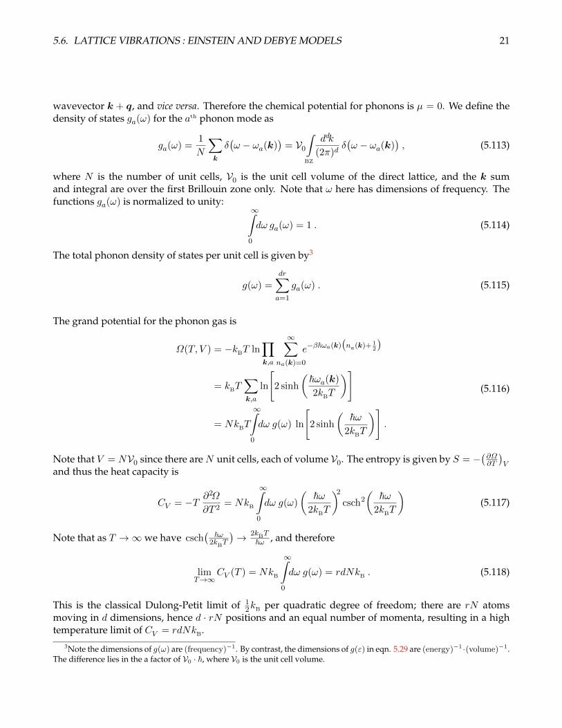


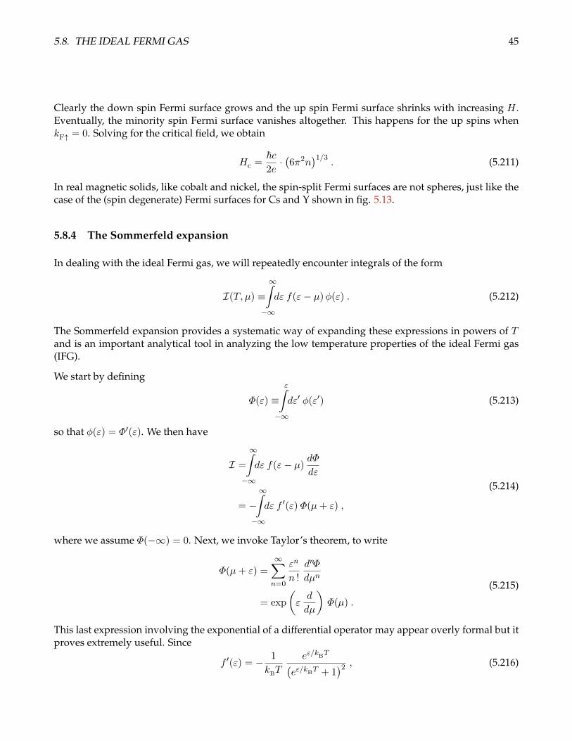


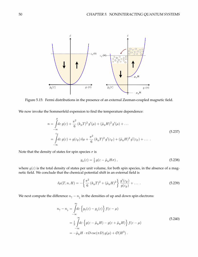


![Rational Canonical Formbuzzard.ups.edu/...spring...canonical-form-present.pdfIntroductionk[x]-modulesMatrix Representation of Cyclic SubmodulesThe Decomposition TheoremRational Canonical](https://static.documents.pub/doc/80x56/6021fbf8c9c62f5c255e87f1/rational-canonical-introductionkx-modulesmatrix-representation-of-cyclic-submodulesthe.jpg)

