Contents Contents i List of Tables iii List of Figures iii 6 Classical Interacting Systems 1 6.1 References .............................................. 1 6.2 Ising Model ............................................. 2 6.2.1 Definition .......................................... 2 6.2.2 Ising model in one dimension .............................. 2 6.2.3 Zero external field ..................................... 3 6.2.4 Chain with free ends ................................... 4 6.2.5 Ising model in two dimensions : Peierls’ argument .................. 5 6.2.6 Two dimensions or one? ................................. 9 6.2.7 High temperature expansion ............................... 10 6.3 Nonideal Classical Gases ..................................... 13 6.3.1 The configuration integral ................................ 13 6.3.2 One-dimensional Tonks gas ............................... 13 6.3.3 Mayer cluster expansion ................................. 15 6.3.4 Lowest order expansion ................................. 19 6.3.5 One-particle irreducible clusters and the virial expansion .............. 21 i
6.23 The polymer chain as a random coil. . . . . . . . . . . . . . . . . . . . . . . . . . . . . . . . 61
6.24 Radius of gyration Rg of polystyrene in a toluene and benzene solvent. . . . . . . . . . . . 66
Chapter 6
Classical Interacting Systems
6.1 References
– M. Kardar, Statistical Physics of Particles (Cambridge, 2007)A superb modern text, with many insightful presentations of key concepts.
– L. E. Reichl, A Modern Course in Statistical Physics (2nd edition, Wiley, 1998)A comprehensive graduate level text with an emphasis on nonequilibrium phenomena.
– M. Plischke and B. Bergersen, Equilibrium Statistical Physics (3rd edition, World Scientific, 2006)An excellent graduate level text. Less insightful than Kardar but still a good modern treatment ofthe subject. Good discussion of mean field theory.
– E. M. Lifshitz and L. P. Pitaevskii, Statistical Physics (part I, 3rd edition, Pergamon, 1980)This is volume 5 in the famous Landau and Lifshitz Course of Theoretical Physics . Though dated,it still contains a wealth of information and physical insight.
– J.-P Hansen and I. R. McDonald, Theory of Simple Liquids (Academic Press, 1990)An advanced, detailed discussion of liquid state physics.
1
2 CHAPTER 6. CLASSICAL INTERACTING SYSTEMS
6.2 Ising Model
6.2.1 Definition
The simplest model of an interacting system consists of a lattice L of sites, each of which contains a spinσi which may be either up (σi = +1) or down (σi = −1). The Hamiltonian is
H = −J∑〈ij〉
σi σj − µ0H∑i
σi . (6.1)
When J > 0, the preferred (i.e. lowest energy) configuration of neighboring spins is that they are aligned,i.e. σi σj = +1. The interaction is then called ferromagnetic. When J < 0 the preference is for anti-alignment, i.e. σi σj = −1, which is antiferromagnetic.
This model is not exactly solvable in general. In one dimension, the solution is quite straightforward.In two dimensions, Onsager’s solution of the model (with H = 0) is among the most celebrated resultsin statistical physics. In higher dimensions the system has been studied by numerical simulations (theMonte Carlo method) and by field theoretic calculations (renormalization group), but no exact solutionsexist.
6.2.2 Ising model in one dimension
Consider a one-dimensional ring of N sites. The ordinary canonical partition function is then
Zring = Tr e−βH
=∑σn
N∏n=1
eβJσnσn+1 eβµ0Hσn
= Tr(RN),
(6.2)
where σN+1 ≡ σ1 owing to periodic (ring) boundary conditions, and where R is a 2× 2 transfer matrix,
are the eigenvalues of R. In the thermodynamic limit, N → ∞, and the λN+ term dominates exponen-tially. We therefore have
F (T,H,N) = −NkBT lnλ+(T,H) . (6.6)
From the free energy, we can compute the magnetization,
M = −(∂F
∂H
)T,N
=Nµ0 sinh(βµ0H)√
sinh2(βµ0H) + e−4βJ(6.7)
and the zero field isothermal susceptibility,
χ(T ) =1
N
∂M
∂H
∣∣∣∣H=0
=µ2
0
kBTe2J/kBT . (6.8)
Note that in the noninteracting limit J → 0 we recover the familiar result for a free spin. The effect of theinteractions at low temperature is to vastly increase the susceptibility. Rather than a set of independentsingle spins, the system effectively behaves as if it were composed of large blocks of spins, where theblock size ξ is the correlation length, to be derived below.
The physical properties of the system are often elucidated by evaluation of various correlation functions.In this case, we define
C(n) ≡⟨σ1 σn+1
⟩=
Tr(σ1Rσ1σ2
· · ·Rσnσn+1σn+1Rσn+1σn+2
· · ·RσNσ1)
Tr(RN)
=Tr(ΣRnΣRN−n
)Tr(RN) ,
(6.9)
where 0 < n < N , and where
Σ =
(1 00 −1
). (6.10)
To compute this ratio, we decompose R in terms of its eigenvectors, writing
R = λ+ |+〉〈+|+ λ− |−〉〈−| . (6.11)
Then
C(n) =λN+ Σ2
++ + λN− Σ2−− +
(λN−n+ λn− + λn+ λ
N−n−
)Σ+−Σ−+
λN+ + λN−, (6.12)
whereΣµµ′ = 〈µ |Σ |µ′ 〉 . (6.13)
6.2.3 Zero external field
Consider the case H = 0, where R = eβJ + e−βJ τx, where τx is the Pauli matrix. Then
| ± 〉 = 1√2
(|↑〉 ± |↓〉
), (6.14)
4 CHAPTER 6. CLASSICAL INTERACTING SYSTEMS
i.e. the eigenvectors of R are
ψ± =1√2
(1±1
), (6.15)
and Σ++ = Σ−− = 0, while Σ± = Σ−+ = 1. The corresponding eigenvalues are
λ+ = 2 cosh(βJ) , λ− = 2 sinh(βJ) . (6.16)
The correlation function is then found to be
C(n) ≡⟨σ1 σn+1
⟩=λN−|n|+ λ
|n|− + λ
|n|+ λ
N−|n|−
λN+ + λN−
=tanh|n|(βJ) + tanhN−|n|(βJ)
1 + tanhN (βJ)
≈ tanh|n|(βJ) (N →∞) .
(6.17)
This result is also valid for n < 0, provided |n| ≤ N . We see that we may write
C(n) = e−|n|/ξ(T ) , (6.18)
where the correlation length is
ξ(T ) =1
ln ctnh(J/kBT ). (6.19)
Note that ξ(T ) grows as T → 0 as ξ ≈ 12 e
2J/kBT .
6.2.4 Chain with free ends
When the chain has free ends, there are (N−1) links, and the partition function is
Zchain =∑σ,σ′
(RN−1
)σσ′
=∑σ,σ′
λN−1
+ ψ+(σ)ψ+(σ′) + λN−1− ψ−(σ)ψ−(σ′)
,
(6.20)
where ψ±(σ) = 〈σ | ± 〉. When H = 0, we make use of eqn. 6.15 to obtain
RN−1 =1
2
(1 11 1
)(2 coshβJ
)N−1+
1
2
(1 −1−1 1
)(2 sinhβJ
)N−1, (6.21)
and thereforeZchain = 2N coshN−1(βJ) . (6.22)
There’s a nifty trick to obtaining the partition function for the Ising chain which amounts to a change ofvariables. We define
νn ≡ σn σn+1 (n = 1 , . . . , N − 1) . (6.23)
6.2. ISING MODEL 5
Thus, ν1 = σ1σ2, ν2 = σ2σ3, etc. Note that each νj takes the values ±1. The Hamiltonian for the chain is
Hchain = −JN−1∑n=1
σn σn+1 = −JN−1∑n=1
νn . (6.24)
The state of the system is defined by the N Ising variables σ1 , ν1 , . . . , νN−1. Note that σ1 doesn’tappear in the Hamiltonian. Thus, the interacting model is recast as N−1 noninteracting Ising spins, andthe partition function is
Zchain = Tr e−βHchain
=∑σ1
∑ν1
· · ·∑νN−1
eβJν1eβJν2 · · · eβJνN−1
=∑σ1
(∑ν
eβJν
)N−1
= 2N coshN−1(βJ) .
(6.25)
6.2.5 Ising model in two dimensions : Peierls’ argument
We have just seen how in one dimension, the Ising model never achieves long-ranged spin order. Thatis, the spin-spin correlation function decays asymptotically as an exponential function of the distancewith a correlation length ξ(T ) which is finite for all > 0. Only for T = 0 does the correlation lengthdiverge. At T = 0, there are two ground states, |↑↑↑↑ · · · ↑ 〉 and |↓↓↓↓ · · · ↓ 〉. To choose between theseground states, we can specify a boundary condition at the ends of our one-dimensional chain, wherewe demand that the spins are up. Equivalently, we can apply a magnetic field H of order 1/N , whichvanishes in the thermodynamic limit, but which at zero temperature will select the ‘all up’ ground state.At finite temperature, there is always a finite probability for any consecutive pair of sites (n, n+1) tobe in a high energy state, i.e. either |↑↓ 〉 or |↓↑ 〉. Such a configuration is called a domain wall, and inone-dimensional systems domain walls live on individual links. Relative to the configurations |↑↑ 〉 and|↓↓ 〉, a domain wall costs energy 2J . For a system with M = xN domain walls, the free energy is
F = 2MJ − kBT ln
(N
M
)= N ·
2Jx+ kBT
[x lnx+ (1− x) ln(1− x)
],
(6.26)
Minimizing the free energy with respect to x, one finds x = 1/(e2J/kBT + 1
), so the equilibrium con-
centration of domain walls is finite, meaning there can be no long-ranged spin order. In one dimension,entropy wins and there is always a thermodynamically large number of domain walls in equilibrium.And since the correlation length for T > 0 is finite, any boundary conditions imposed at spatial infinitywill have no thermodynamic consequences since they will only be ‘felt’ over a finite range.
As we shall discuss in the following chapter, this consideration is true for any system with sufficientlyshort-ranged interactions and a discrete global symmetry. Another example is the q-state Potts model,
H = −J∑〈ij〉
δσi,σj− h
∑i
δσi,1. (6.27)
6 CHAPTER 6. CLASSICAL INTERACTING SYSTEMS
+
−
+ + + + + + + + + + + + + + +
+ + + + + + + + + +
+ + + + + + + + + + +
+ + + + + + + + + + + +
+ + + + + + + + + + + + + +
+ + + + + + + + + + + + +
+ + + + + + + + + +
+ + + + + + + + + + +
+ + + + + + + + + +
+ + + + + + + +
+ + + + + + + + + +
+ + + + + + + + + + + + +
+ + + + + + + + + + + + + +
+ + + + + + + + + +
+ + + + + + + + + + + + + + +
−−
−−−
−−−
−−−
−−−
−−−
−−−
−−
−−
−−
−−
−−
−
−
− −
−
−
−−
−−
−
−
−
−−
−
+
−
+ + + + + + + + + + + + + + +
+ + + + + + + + + +
+ + + + + + + + + + +
+ + + + + + + + + + + +
+ + + + + + + + + + + + + +
+ + + + + + + + + + + + +
+ + + + + + + +
+ + + + + + + + + + +
+ + + + + + + + +
+ + + + + + +
+ + + + + + + + +
+ + + + + + + + + +
+ + + + + + + + + + + + + +
+ + + + + + + + + +
+ + + + + + + + + + + + + + +
−−
−−−
−−−
−−−
−−−
−−−
−−−
−−
−−
−−
−−
−−
−
−
− −
−
−
−−
−−
−
−
−
−−
−
−−
−−
−−−
−
−
−
Figure 6.1: Clusters and boundaries for the square lattice Ising model. Left panel: a configuration Γwhere the central spin is up. Right panel: a configuration Cγ Γ where the interior spins of a new loopγ containing the central spin have been flipped.
Here, the spin variables σi take values in the set 1, 2, . . . , q on each site. The equivalent of an externalmagnetic field in the Ising case is a field h which prefers a particular value of σ (σ = 1 in the aboveHamiltonian). See the appendix in §6.8 for a transfer matrix solution of the one-dimensional Potts model.
What about higher dimensions? A nifty argument due to R. Peierls shows that there will be a finitetemperature phase transition for the Ising model on the square lattice1. Consider the Ising model, inzero magnetic field, on a Nx × Ny square lattice, with Nx,y → ∞ in the thermodynamic limit. Alongthe perimeter of the system we impose the boundary condition σi = +1. Any configuration of the spinsmay then be represented uniquely in the following manner. Start with a configuration in which all spinsare up. Next, draw a set of closed loops on the lattice. By definition, the loops cannot share any linksalong their boundaries, i.e. each link on the lattice is associated with at most one such loop. Now flip allthe spins inside each loop from up to down. Identify each such loop configuration with a label Γ . Thepartition function is
Z = Tr e−βH =∑Γ
e−2βJLΓ , (6.28)
where LΓ is the total perimeter of the loop configuration Γ . The domain walls are now loops, ratherthan individual links, but as in the one-dimensional case, each link of each domain wall contributes anenergy +2J relative to the ground state.
Now we wish to compute the average magnetization of the central site (assume Nx,y are both odd, sothere is a unique central site). This is given by the difference P+(0) − P−(0), where Pµ(0) =
⟨δσ0 , µ
⟩is
the probability that the central spin has spin polarization µ. If P+(0) > P−(0), then the magnetization
1Here we modify slightly the discussion in chapter 5 of the book by L. Peliti.
6.2. ISING MODEL 7
per site m = P+(0)− P−(0) is finite in the thermodynamic limit, and the system is ordered. Clearly
P+(0) =1
Z
∑Γ∈Σ+
e−2βJLΓ , (6.29)
where the restriction on the sum indicates that only those configurations where the central spin is up(σ0 = +1) are to be included. (see fig. 6.1a). Similarly,
P−(0) =1
Z
∑Γ∈Σ−
e−2βJL
Γ , (6.30)
where only configurations in which σ0 = −1 are included in the sum. Here we have defined
Σ± =Γ∣∣ σ0 = ±
. (6.31)
I.e. Σ+(Σ−) is the set of configurations Γ in which the central spin is always up (down). Consider nowthe construction in fig. 6.1b. Any loop configuration Γ ∈ Σ− may be associated with a unique loopconfiguration Γ ∈ Σ+ by reversing all the spins within the loop of Γ which contains the origin. Notethat the map from Γ to Γ is many-to-one. That is, we can write Γ = Cγ Γ , where Cγ overturns thespins within the loop γ, with the conditions that (i) γ contains the origin, and (ii) none of the links in theperimeter of γ coincide with any of the links from the constituent loops of Γ . Let us denote this set ofloops as ΥΓ :
ΥΓ =γ : 0 ∈ int(γ) and γ ∩ Γ = ∅
. (6.32)
Then
m = P+(0)− P−(0) =1
Z
∑Γ∈Σ+
e−2βJLΓ
(1−
∑γ∈ΥΓ
e−2βJLγ
). (6.33)
If we can prove that∑
γ∈ΥΓe−2βJLγ < 1, then we will have established that m > 0. Let us ask: how
many loops γ are there in ΥΓ with perimeter L? We cannot answer this question exactly, but we canderive a rigorous upper bound for this number, which, following Peliti, we call g(L). We claim that
g(L) <2
3L· 3L ·
(L
4
)2
=L
24· 3L . (6.34)
To establish this bound, consider any site on such a loop γ. Initially we have 4 possible directions toproceed to the next site, but thereafter there are only 3 possibilities for each subsequent step, since theloop cannot run into itself. This gives 4 · 3L−1 possibilities. But we are clearly overcounting, since anypoint on the loop could have been chosen as the initial point, and moreover we could have started byproceeding either clockwise or counterclockwise. So we are justified in dividing this by 2L. We arestill overcounting, because we have not accounted for the constraint that γ is a closed loop, nor thatγ ∩ Γ = ∅. We won’t bother trying to improve our estimate to account for these constraints. However,we are clearly undercounting due to the fact that a given loop can be translated in space so long as theorigin remains within it. To account for this, we multiply by the area of a square of side length L/4,which is the maximum area that can be enclosed by a loop of perimeter L. We therefore arrive at eqn.
8 CHAPTER 6. CLASSICAL INTERACTING SYSTEMS
0 -1
-2-3-4-5
-6
-7
1
2 3 4 5
6
7
8
-8 -9
910
-10
11
-11 -12 -13
-14
-15
-16
-17
-18-19-20-21-22-23-24-25
-26
-27
-28
-29
-30
-31
-32 -33 -34 -35
1213
14
15
16
17
18 19 20 21 22 23 24 25
26
27
28
29
30
31
32333435
Figure 6.2: A two-dimensional square lattice mapped onto a one-dimensional chain.
6.34. Finally, we note that the smallest possible value of L is L = 4, corresponding to a square enclosingthe central site alone. Therefore
∑γ∈ΥΓ
e−2βJLγ <1
12
∞∑k=2
k ·(3 e−2βJ
)2k=
x4 (2− x2)
12 (1− x2)2≡ r , (6.35)
where x = 3 e−2βJ . Note that we have accounted for the fact that the perimeter L of each loop γ mustbe an even integer. The sum is smaller than unity provided x < x0 = 0.869756 . . ., hence the system isordered provided
kBT
J<
2
ln(3/x0)= 1.61531 . (6.36)
The exact result is kBTc = 2J/ sinh−1(1) = 2.26918 . . . The Peierls argument has been generalized tohigher dimensional lattices as well2.
With a little more work we can derive a bound for the magnetization. We have shown that
P−(0) =1
Z
∑Γ∈Σ+
e−2βJLΓ∑γ∈ΥΓ
e−2βJLγ < r · 1
Z
∑Γ∈Σ+
e−2βJLΓ = r P+(0) . (6.37)
Thus,1 = P+(0) + P−(0) < (1 + r)P+(0) (6.38)
and thereforem = P+(0)− P−(0) > (1− r)P+(0) >
1− r1 + r
, (6.39)
where r(T ) is given in eqn. 6.35.
2See. e.g. J. L. Lebowitz and A. E. Mazel, J. Stat. Phys. 90, 1051 (1998).
6.2. ISING MODEL 9
6.2.6 Two dimensions or one?
We showed that the one-dimensional Ising model has no finite temperature phase transition, and isdisordered at any finite temperature T , but in two dimensions on the square lattice there is a finitecritical temperature Tc below which there is long-ranged order. Consider now the construction depictedin fig. 6.2, where the sites of a two-dimensional square lattice are mapped onto those of a linear chain3.Clearly we can elicit a one-to-one mapping between the sites of a two-dimensional square lattice andthose of a one-dimensional chain. That is, the two-dimensional square lattice Ising model may be writtenas a one-dimensional Ising model, i.e.
H = −J
squarelattice∑〈ij〉
σi σj = −
linearchain∑n,n′
Jnn′ σn σn′ . (6.40)
How can this be consistent with the results we have just proven?
The fly in the ointment here is that the interaction along the chain Jn,n′ is long-ranged. This is apparentfrom inspecting the site labels in fig. 6.2. Note that site n = 15 is linked to sites n′ = 14 and n′ = 16,but also to sites n′ = −6 and n′ = −28. With each turn of the concentric spirals in the figure, the rangeof the interaction increases. To complicate matters further, the interactions are no longer translationallyinvariant, i.e. Jnn′ 6= J(n − n′). But it is the long-ranged nature of the interactions on our contrivedone-dimensional chain which spoils our previous energy-entropy argument, because now the domainwalls themselves interact via a long-ranged potential. Consider for example the linear chain with Jn,n′ =
J |n− n′|−α, where α > 0. Let us compute the energy of a domain wall configuration where σn = +1 ifn > 0 and σn = −1 if n ≤ 0. The domain wall energy is then
∆ =∞∑m=0
∞∑n=1
2J
|m+ n|α. (6.41)
Here we have written one of the sums in terms of m = −n′. For asymptotically large m and n, we canwriteR = (m,n) and we obtain an integral over the upper right quadrant of the plane:
∞∫1
dR R
π/2∫0
dφ2J
Rα (cosφ+ sinφ)α= 2−α/2
π/4∫−π/4
dφ
cosαφ
∞∫1
dR
Rα−1. (6.42)
The φ integral is convergent, but the R integral diverges for α ≤ 2. For a finite system, the upperbound on the R integral becomes the system size L. For α > 2 the domain wall energy is finite in thethermodynamic limit L → ∞. In this case, entropy again wins. I.e. the entropy associated with a singledomain wall is kB lnL, and therefore F = E − kBT is always lowered by having a finite density ofdomain walls. For α < 2, the energy of a single domain wall scales as L2−α. It was first proven by F. J.Dyson in 1969 that this model has a finite temperature phase transition provided 1 < α < 2. There is notransition for α < 1 or α > 2. The case α = 2 is special, and is discussed as a special case in the beautifulrenormalization group analysis by J. M. Kosterlitz in Phys. Rev. Lett. 37, 1577 (1976).
3A corresponding mapping can be found between a cubic lattice and the linear chain as well.
10 CHAPTER 6. CLASSICAL INTERACTING SYSTEMS
6.2.7 High temperature expansion
Consider once again the ferromagnetic Ising model in zero field (H = 0), but on an arbitrary lattice. Thepartition function is
Z = Tr eβJ∑〈ij〉 σi σj =
(coshβJ
)NL Tr
∏〈ij〉
(1 + xσi σj
), (6.43)
where x = tanhβJ and NL is the number of links. For regular lattices, NL = 12zN , where N is the
number of lattice sites and z is the lattice coordination number, i.e. the number of nearest neighbors foreach site. We have used
eβJσσ′
= coshβJ ·
1 + σσ′ tanhβJ
=
e+βJ if σσ′ = +1
e−βJ if σσ′ = −1 .(6.44)
We expand eqn. 6.43 in powers of x, resulting in a sum of 2NL terms, each of which can be representedgraphically in terms of so-called lattice animals. A lattice animal is a distinct (including reflections androtations) arrangement of adjacent plaquettes on a lattice. In order that the trace not vanish, only suchconfigurations and their compositions are permitted. This is because each σi for every given site i mustoccur an even number of times in order for a given term in the sum not to vanish. For all such terms,the trace is 2N . Let Γ represent a collection of lattice animals, and gΓ the multiplicity of Γ . Then
Z = 2N(coshβJ
)NL∑Γ
gΓ(tanhβJ
)LΓ , (6.45)
where LΓ is the total number of sites in the diagram Γ , and gΓ is the multiplicity of Γ . Since x vanishesas T →∞, this procedure is known as the high temperature expansion (HTE).
For the square lattice, he enumeration of all lattice animals with up to order eight is given in fig. 6.3.For the diagram represented as a single elementary plaquette, there are N possible locations for thelower left vertex. For the 2 × 1 plaquette animal, one has g = 2N , because there are two inequivalentorientations as well as N translations. For two disjoint elementary squares, one has g = 1
2N(N − 5),which arises from subtracting 5N ‘illegal’ configurations involving double lines (remember each linkin the partition sum appears only once!), shown in the figure, and finally dividing by two because theindividual squares are identical. Note that N(N − 5) is always even for any integer value of N . Thus, tolowest interesting order on the square lattice,
Z = 2N(coshβJ
)2N1 +Nx4 + 2Nx6 +
(7− 5
2
)Nx8 + 1
2N2x8 +O(x10)
. (6.46)
The free energy is therefore
F = −kBT ln 2 +NkBT ln(1− x2)−NkBT[x4 + 2x6 + 9
2 x8 +O(x10)
]= NkBT ln 2−NkBT
x2 + 3
2 x4 + 7
3 x6 + 19
4 x8 +O(x10)
,
(6.47)
again with x = tanhβJ . Note that we’ve substituted cosh2βJ = 1/(1 − x2) to write the final result as apower series in x. Notice that theO(N2) factor in Z has cancelled upon taking the logarithm, so the freeenergy is properly extensive.
6.2. ISING MODEL 11
Figure 6.3: HTE diagrams on the square lattice and their multiplicities.
Note that the high temperature expansion for the one-dimensional Ising chain yields
in agreement with the transfer matrix calculations. In higher dimensions, where there is a finite tem-perature phase transition, one typically computes the specific heat c(T ) and tries to extract its singularbehavior in the vicinity of Tc, where c(T ) ∼ A (T −Tc)
−α. Since x(T ) = tanh(J/kBT ) is analytic in T , wehave c(x) ∼ A′ (x− xc)
−α, where xc = x(Tc). One assumes xc is the singularity closest to the origin andcorresponds to the radius of convergence of the high temperature expansion. If we write
c(x) =
∞∑n=0
an xn ∼ A′′
(1− x
xc
)−α, (6.49)
then according to the binomial theorem we should expect
anan−1
=1
xc
[1− 1− α
n
]. (6.50)
Thus, by plotting an/an−1 versus 1/n, one extracts 1/xc as the intercept, and (α− 1)/xc as the slope.
12 CHAPTER 6. CLASSICAL INTERACTING SYSTEMS
Figure 6.4: HTE diagrams for the numerator Ykl of the correlation functionCkl. The blue path connectingsites k and l is the string. The remaining red paths are all closed loops.
High temperature expansion for correlation functions
Can we also derive a high temperature expansion for the spin-spin correlation function Ckl = 〈σk σl〉 ?Yes we can. We have
Ckl =Tr[σk σl e
βJ∑〈ij〉 σi σj
]Tr[eβJ
∑〈ij〉 σi σj
] ≡YklZ
. (6.51)
Recall our analysis of the partition function Z. We concluded that in order for the trace not to vanish,the spin variable σi on each site i must occur an even number of times in the expansion of the product.Similar considerations hold for Ykl, except now due to the presence of σk and σl, those variables nowmust occur an odd number of times when expanding the product. It is clear that the only nonvanishingdiagrams will be those in which there is a finite string connecting sites k and l, in addition to the usualclosed HTE loops. See fig. 6.4 for an instructive sketch. One then expands both Ykl as well as Z inpowers of x = tanhβJ , taking the ratio to obtain the correlator Ckl. At high temperatures (x → 0),both numerator and denominator are dominated by the configurations Γ with the shortest possibletotal perimeter. For Z, this means the trivial path Γ = ∅, while for Ykl this means finding the shortestlength path from k to l. (If there is no straight line path from k to l, there will in general be several suchminimizing paths.) Note, however, that the presence of the string between sites k and l complicatesthe analysis of gΓ for the closed loops, since none of the links of Γ can intersect the string. It is worthstressing that this does not mean that the string and the closed loops cannot intersect at isolated sites,but only that they share no common links; see once again fig. 6.4.
6.3. NONIDEAL CLASSICAL GASES 13
6.3 Nonideal Classical Gases
Let’s switch gears now and return to the study of continuous classical systems described by a Hamilto-nian H
(xi, pi
). In the next chapter, we will see how the critical properties of classical fluids can in
fact be modeled by an appropriate lattice gas Ising model, and we’ll derive methods for describing theliquid-gas phase transition in such a model.
6.3.1 The configuration integral
Consider the ordinary canonical partition function for a nonideal system of identical point particlesinteracting via a central two-body potential u(r). We work in the ordinary canonical ensemble. TheN -particle partition function is
Z(T, V,N) =1
N !
∫ N∏i=1
ddpi ddxi
hde−H/kBT
=λ−NdT
N !
∫ N∏i=1
ddxi exp
(− 1
kBT
∑i<j
u(|xi − xj |
)).
(6.52)
Here, we have assumed a many body Hamiltonian of the form
H =N∑i=1
p2i
2m+∑i<j
u(|xi − xj |
), (6.53)
in which massive nonrelativistic particles interact via a two-body central potential. As before, λT =√2π~2/mkBT is the thermal wavelength. We can now write
Z(T, V,N) = λ−NdT QN (T, V ) , (6.54)
where the configuration integral QN (T, V ) is given by
QN (T, V ) =1
N !
∫ddx1 · · ·
∫ddxN
∏i<j
e−βu(rij) . (6.55)
There are no general methods for evaluating the configurational integral exactly.
6.3.2 One-dimensional Tonks gas
The Tonks gas is a one-dimensional generalization of the hard sphere gas. Consider a one-dimensionalgas of indistinguishable particles of mass m interacting via the potential
u(x− x′) =
∞ if |x− x′| < a
0 if |x− x′| ≥ a .(6.56)
14 CHAPTER 6. CLASSICAL INTERACTING SYSTEMS
Thus, the Tonks gas may be considered to be a gas of hard rods. The above potential guarantees thatthe portion of configuration space in which any rods overlap is forbidden in this model4. Let the gas beplaced in a finite volume L. The hard sphere nature of the particles means that no particle can get withina distance 1
2a of the ends at x = 0 and x = L. That is, there is a one-body potential v(x) acting as well,where
v(x) =
∞ if x < 1
2a
0 if 12a ≤ x ≤ L−
12a
∞ if x > L− 12a .
(6.57)
The configuration integral of the 1D Tonks gas is given by
QN (T, L) =1
N !
L∫0
dx1 · · ·L∫
0
dxN χ(x1, . . . , xN ) , (6.58)
where χ = e−U/kBT is zero if any two ‘rods’ (of length a) overlap, or if any rod overlaps with eitherboundary at x = 0 and x = L, and χ = 1 otherwise. Note that χ does not depend on temperature.Without loss of generality, we can integrate over the subspace where x1 < x2 < · · · < xN and thenmultiply the result by N ! . Clearly xj must lie to the right of xj−1 + a and to the left of Yj ≡ L − (N −j)a− 1
2a. Thus, the configurational integral is
QN (T, L) =
Y1∫a/2
dx1
Y2∫x1+a
dx2 · · ·
YN∫xN−1+a
dxN
=
Y1∫a/2
dx1
Y2∫x1+a
dx2 · · ·
YN−1∫xN−2+a
dxN−1
(YN−1 − xN−1
)
=
Y1∫a/2
dx1
Y2∫x1+a
dx2 · · ·
YN−2∫xN−3+a
dxN−212
(YN−2 − xN−2
)2= · · ·
=1
N !
(X1 − 1
2a)N
=1
N !(L−Na)N .
(6.59)
The partition function is Z(T, L,N) = λ−NT QN (T, L) , and so the free energy is
F = −kBT lnZ = −NkBT
− lnλT + 1 + ln
(L
N− a)
, (6.60)
where we have used Stirling’s rule to write lnN ! ≈ N lnN −N . The pressure is
p = −∂F∂L
=kBTLN − a
=nkBT
1− na, (6.61)
4Not that I personally think there’s anything wrong with that.
6.3. NONIDEAL CLASSICAL GASES 15
where n = N/L is the one-dimensional density. Note that the pressure diverges as n approaches 1/a.The usual one-dimensional ideal gas law, pL = NkBT , is replaced by pLeff = NkBT , where Leff = L−Nais the ‘free’ volume obtained by subtracting the total ”excluded volume”Na from the original volume L.Note the similarity here to the van der Waals equation of state, (p+av−2)(v−b) = RT , where v = NAV/Nis the molar volume. Defining a ≡ a/N2
A and b ≡ b/NA, we have
p+ an2 =nkBT
1− bn, (6.62)
where n = NA/v is the number density. The term involving the constant a is due to the long-rangedattraction of atoms due to their mutual polarizability. The term involving b is an excluded volumeeffect. The Tonks gas models only the latter.
6.3.3 Mayer cluster expansion
Let us return to the general problem of computing the configuration integral. Consider the functione−βuij , where uij ≡ u(|xi − xj |). We assume that at very short distances there is a strong repulsionbetween particles, i.e. uij →∞ as rij = |xi−xj | → 0, and that uij → 0 as rij →∞. Thus, e−βuij vanishesas rij → 0 and approaches unity as rij →∞. For our purposes, it will prove useful to define the function
f(r) = e−βu(r) − 1 , (6.63)
called the Mayer function after Josef Mayer. We may now write
QN (T, V ) =1
N !
∫ddx1 · · ·
∫ddxN
∏i<j
(1 + fij
). (6.64)
A typical potential we might consider is the semi-phenomenological Lennard-Jones potential,
u(r) = 4 ε
(σr
)12−(σr
)6. (6.65)
This accounts for a long-distance attraction due to mutually induced electric dipole fluctuations, anda strong short-ranged repulsion, phenomenologically modelled with a r−12 potential, which mimics ahard core due to overlap of the atomic electron distributions. Setting u′(r) = 0 we obtain r∗ = 21/6 σ ≈1.12246σ at the minimum, where u(r∗) = −ε. In contrast to the Boltzmann weight e−βu(r), the Mayerfunction f(r) vanishes as r → ∞, behaving as f(r) ∼ −βu(r). The Mayer function also depends ontemperature. Sketches of u(r) and f(r) for the Lennard-Jones model are shown in fig. 6.5.
The Lennard-Jones potential5 is realistic for certain simple fluids, but it leads to a configuration integralwhich is in general impossible to evaluate. Indeed, even a potential as simple as that of the hard sphere
5Disambiguation footnote: Take care not to confuse Philipp Lenard (Hungarian-German, cathode ray tubes, Nazi), Alfred-Marie Lienard (French, Lienard-Wiechert potentials, not a Nazi), John Lennard-Jones (British, molecular structure, definitelynot a Nazi), and Lynyrd Skynyrd (American, ”Free Bird”, possibly killed by Nazis in 1977 plane crash). I thank my colleagueOleg Shpyrko for setting me straight on this.
the weak attractive tail and the strong repulsive core. Top panel: Mayer function f(r, T ) = e−u(r)/kBT −1for kBT = 0.8 ε (blue), kBT = 1.5 ε (green), and kBT = 5 ε (red).
gas is intractable in more than one space dimension. We can however make progress by deriving aseries expansion for the equation of state in powers of the particle density. This is known as the virialexpansion. As was the case when we investigated noninteracting quantum statistics, it is convenient towork in the grand canonical ensemble and to derive series expansions for the density n(T, z) and thepressure p(T, z) in terms of the fugacity z, then solve for z(T, n) to obtain p(T, n). These expansions interms of fugacity have a nifty diagrammatic interpretation, due to Mayer.
We begin by expanding the product in eqn. 6.64 as∏i<j
(1 + fij
)= 1 +
∑i<j
fij +∑
i<j , k<l(ij)6=(kl)
fij fkl + . . . . (6.66)
As there are 12N(N − 1) possible pairings, there are 2N(N−1)/2 terms in the expansion of the above
product. Each such term may be represented by a graph, as shown in fig. 6.7. For each such term,we draw a connection between dots representing different particles i and j if the factor fij appears inthe term under consideration. The contribution for any given graph may be written as a product overcontributions from each of its disconnected component clusters. For example, in the case of the term infig. 6.7, the contribution to the configurational integral would be
∆Q =V N−11
N !
∫ddx1 d
dx4 ddx7 d
dx9 f1,4 f4,7 f4,9 f7,9
×∫ddx2 d
dx5 ddx6 f2,5 f2,6 ×
∫ddx3 d
dx10 f3,10 ×∫ddx8 d
dx11 f8,11 .
(6.67)
We will refer to a given product of Mayer functions which arises from this expansion as a term.
6.3. NONIDEAL CLASSICAL GASES 17
Figure 6.6: Left: John Lennard-Jones. Center: Catherine Zeta-Jones. Right: James Earl Jones.
The particular labels we assign to each vertex of a given graph don’t affect the overall value of the graph.Now a given unlabeled graph consists of a certain number of connected subgraphs. For a system withN particles, we may then write
N =∑γ
mγ nγ , (6.68)
where γ ranges over all possible connected subgraphs, and
mγ = number of connected subgraphs of type γ in the unlabeled graph
nγ = number of vertices in the connected subgraph γ .
Note that the single vertex • counts as a connected subgraph, with n• = 1. We now ask: how many waysare there of assigning theN labels to theN vertices of a given unlabeled graph? One might first thing theanswer is simply N !, however this is too big, because different assignments of the labels to the verticesmay not result in a distinct graph. To see this, consider the examples in fig. 6.8. In the first example, anunlabeled graph with four vertices consists of two identical connected subgraphs. Given any assignmentof labels to the vertices, then, we can simply exchange the two subgraphs and get the same term. So weshould divide N ! by the product
∏γmγ ! . But even this is not enough, because within each connected
subgraph γ there may be permutations which leave the integrand unchanged, as shown in the secondand third examples in fig. 6.8. We define the symmetry factor sγ as the number of permutations ofthe labels which leaves a given connected subgraphs γ invariant. Examples of symmetry factors areshown in fig. 6.9. Consider, for example, the third subgraph in the top row. Clearly one can rotate
Figure 6.7: Diagrammatic interpretation of a term involving a product of eight Mayer functions.
18 CHAPTER 6. CLASSICAL INTERACTING SYSTEMS
Figure 6.8: Different assignations of labels to vertices may not result in a distinct term in the expansionof the configuration integral.
the figure about its horizontal symmetry axis to obtain a new labeling which represents the same term.This twofold axis is the only symmetry the diagram possesses, hence sγ = 2. For the first diagram inthe second row, one can rotate either of the triangles about the horizontal symmetry axis. One can alsorotate the figur e in the plane by 180 so as to exchange the two triangles. Thus, there are 2 × 2 × 2 = 8
symmetry operations which result in the same term, and sγ = 8. Finally, the last subgraph in the secondrow consists of five vertices each of which is connected to the other four. Therefore any permutation ofthe labels results in the same term, and sγ = 5! = 120. In addition to dividing by the product
∏γmγ !,
we must then also divide by∏γ s
mγγ .
We can now write the partition function as
Z =λ−NdT
N !
∑mγ
N !∏mγ ! s
mγγ
·∏γ
(∫ddx1 · · · d
dxnγ
γ∏i<j
fij
)mγ· δN ,
∑mγnγ
= λ−NdT
∑mγ
∏γ
(V bγ(T )
)mγmγ !
· δN ,∑mγnγ
(6.69)
where the product∏γi<j fij is over all links in the subgraph γ. The final Kronecker delta enforces the
constraint N =∑
γmγ nγ . We have defined the cluster integrals bγ as
bγ(T ) ≡ 1
sγ· 1
V
∫ddx1 · · · d
dxnγ
γ∏i<j
fij , (6.70)
where we assume the limit V → ∞. Since fij = f(|xi − xj |
), the product
∏γi<j fij is invariant under
simultaneous translation of all the coordinate vectors by any constant vector, and hence the integral over
6.3. NONIDEAL CLASSICAL GASES 19
the nγ position variables contains exactly one factor of the volume, which cancels with the prefactor inthe above definition of bγ . Thus, each cluster integral is intensive6, scaling as V 0.
If we compute the grand partition function, then the fixed N constraint is relaxed, and we can do thesums:
Ξ = e−βΩ =∑mγ
(eβµ λ−dT
)∑mγnγ∏γ
1
mγ !
(V bγ
)mγ=∏γ
∞∑mγ=0
1
mγ !
(eβµ λ−dT
)mγ nγ(V bγ
)mγ= exp
(V∑γ
(eβµ λ−dT
)nγ bγ) .(6.71)
Thus,Ω(T, V, µ) = −V kBT
∑γ
(eβµ λ−dT
)nγ bγ(T ) , (6.72)
and we can write
p = kBT∑γ
(zλ−dT
)nγ bγ(T )
n =∑γ
nγ(zλ−dT
)nγ bγ(T ) ,(6.73)
where z = exp(βµ) is the fugacity, and where b• ≡ 1. As in the case of ideal quantum gas statisticalmechanics, we can systematically invert the relation n = n(z, T ) to obtain z = z(n, T ), and then insertthis into the equation for p(z, T ) to obtain the equation of state p = p(n, T ). This yields the virial expansionof the equation of state,
p = nkBT
1 +B2(T )n+B3(T )n2 + . . .. (6.74)
6.3.4 Lowest order expansion
We have
b−(T ) =1
2V
∫ddx1
∫ddx2 f
(|x1 − x2|
)= 1
2
∫ddr f(r)
(6.75)
and
b∧(T ) =1
2V
∫ddx1
∫ddx2
∫ddx3 f
(|x1 − x2|
)f(|x1 − x3|
)= 1
2
∫ddr
∫ddr′ f(r) f(r′) = 2
(b−)2 (6.76)
6We assume that the long-ranged behavior of f(r) ≈ −βu(r) is integrable.
20 CHAPTER 6. CLASSICAL INTERACTING SYSTEMS
Figure 6.9: The symmetry factor sγ for a connected subgraph γ is the number of permutations of itsindices which leaves the term
∏(ij)∈γ fij invariant.
and
b4(T ) =1
6V
∫ddx1
∫ddx2
∫ddx3 f
(|x1 − x2|
)f(|x1 − x3|
)f(|x2 − x3|
)= 1
6
∫ddr
∫ddr′ f(r) f(r′) f
(|r − r′|
).
(6.77)
We may now write
p = kBTzλ−dT +
(zλ−dT
)2b−(T ) +
(zλ−dT
)3 · (b∧ + b4)
+O(z4)
n = zλ−dT + 2(zλ−dT
)2b−(T ) + 3
(zλ−dT
)3 · (b∧ + b4)
+O(z4)(6.78)
We invert by writingzλ−dT = n+ α2 n
2 + α3 n3 + . . . (6.79)
and substituting into the equation for n(z, T ), yielding
Note that b∧ does not contribute to B2 – only 4 appears. As we shall see, this is because the virialcoefficientsBj involve only cluster integrals bγ for one-particle irreducible clusters, i.e. those clusters whichremain connected if any of the vertices plus all its links are removed.
6.3.5 One-particle irreducible clusters and the virial expansion
We start with eqn. 6.73 for p(T, z) and n(T, z),
p = kBT∑γ
(zλ−dT
)nγ bγ(T )
n =∑γ
nγ(zλ−dT
)nγ bγ(T ) ,(6.85)
where bγ(T ) for the connected cluster γ is given by
bγ(T ) ≡ 1
sγ· 1
V
∫ddx1 · · · d
dxnγ
γ∏i<j
fij . (6.86)
It is convenient to work with dimensionless quantities, using λdT as the unit of volume. To this end,define
ν ≡ nλdT , π ≡ pλdT , cγ(T ) ≡ bγ(T )(λdT)nγ−1
, (6.87)
so that
βπ =∑γ
cγ znγ =
∞∑`=1
d` z` , ν =
∑γ
nγcγ znγ =
∞∑l=1
` d` z` , (6.88)
whered` =
∑γ
cγ δnγ , ` (6.89)
is the sum over all connected clusters with ` vertices. Here and henceforth, the functional dependenceon T is implicit; π and ν are regarded here as explicit functions of z. We can, in principle, invert to obtainz(ν). Let us write this inverse as
z(ν) = ν exp
(−∞∑k=1
βk νk
). (6.90)
Ultimately we need to obtain expressions for the coefficients βk, but let us first assume the above formand use it to write π in terms of ν. We have
βπ =
∞∑`=1
d` z` =
z∫0
dz
∞∑l=1
` d` z`−1 =
ν∫0
dνdz
dν
ν
z=
ν∫0
dνd ln z
d ln ν
=
ν∫0
dν
(1−
∞∑k=1
k βk νk
)= ν −
∞∑k=1
k βkk + 1
νk+1 ≡∞∑k=1
Bk νk ,
(6.91)
22 CHAPTER 6. CLASSICAL INTERACTING SYSTEMS
where Bk = Bk λ−d(k−1)T is the dimensionless kth virial coefficient. Thus, Bk=1 = 1 and
Bk = −k − 1
kβk−1 (6.92)
for k > 1. We may also obtain the cluster integrals d` in terms of the βk . To this end, note that `2d` is thecoefficient of z` in the function z dν/dz , hence
`2d` =
∮dz
2πiz
1
z`
(zdν
dz
)=
∮dν
2πiz−` =
∮dν
2πi
1
ν`
∞∏k=1
e`βkνk
=
∮dν
2πi
1
ν`
∑mk
∞∏k=1
(` βk)mk
mk!νkmk =
∑mk
δ∑k kmk , `−1
∞∏k=1
(` βk)mk
mk!.
(6.93)
Irreducible clusters
The clusters which contribute to d` are all connected, by definition. However, it is useful to make afurther distinction based on the topology of connected clusters and define a connected cluster γ to beirreducible if, upon removing any site in γ and all the links connected to that site, the remaining sites ofthe cluster are still connected. The situation is depicted in Fig. 6.10. For a reducible cluster γ, the integralcγ is proportional to a product of cluster integrals over its irreducible components. Let us define the set
Figure 6.10: Connected versus irreducible clusters. Clusters (a) through (d) are irreducible in that theyremain connected if any component site and its connecting links are removed. Cluster (e) is connected,but is reducible. Its integral cγ may be reduced to a product over its irreducible components, each shownin a unique color.
6.3. NONIDEAL CLASSICAL GASES 23
Γ` as the set of all irreducible clusters of ` vertices. It turns out that
βk(T ) =1
V λ(k−1)dT
1
k!
∑γ∈Γk+1
∫ddx1 · · ·
∫ddxk
γ∏〈ij〉
fij (6.94)
Thus, the virial coefficients Bj(T ) are obtained by summing a restricted set of cluster integrals, viz.
Bj(T ) = −k − 1
kβk−1(T )λ
(k−1)dT . (6.95)
In the end, it turns out we don’t need the symmetry factors at all!
6.3.6 Cookbook recipe
Just follow these simple steps!
• The pressure and number density are written as an expansion over unlabeled connected clustersγ, viz.
βp =∑γ
(zλ−dT
)nγ bγn =
∑γ
nγ(zλ−dT
)nγ bγ . (6.96)
• For each term in each of these sums, draw the unlabeled connected cluster γ.
• Assign labels 1 , 2 , . . . , nγ to the vertices, where nγ is the total number of vertices in the cluster γ.It doesn’t matter how you assign the labels.
• Write down the product∏γi<j fij . The factor fij appears in the product if there is a link in your
(now labeled) cluster between sites i and j.
• The symmetry factor sγ is the number of elements of the symmetric group Snγ which leave theproduct
∏γi<j fij invariant. The identity permutation leaves the product invariant, so sγ ≥ 1.
• The cluster integral is
bγ(T ) ≡ 1
sγ· 1
V
∫ddx1 · · · d
dxnγ
γ∏i<j
fij . (6.97)
Due to translation invariance, bγ(T ) ∝ V 0. One can therefore set xnγ ≡ 0, eliminate the volumefactor from the denominator, and perform the integral over the remaining nγ−1 coordinates.
• This procedure generates expansions for p(T, z) and n(T, z) in powers of the fugacity z = eβµ. Toobtain something useful like p(T, n), we invert the equation n = n(T, z) to find z = z(T, n), and
24 CHAPTER 6. CLASSICAL INTERACTING SYSTEMS
then substitute into the equation p = p(T, z) to obtain p = p(T, z(T, n)
)= p(T, n). The result is the
virial expansion,p = nkBT
1 +B2(T )n+B3(T )n2 + . . .
, (6.98)
where
Bk(T ) = − 1
k(k − 2)!
∑γ∈Γk
∫ddx1 · · ·
∫ddxk−1
γ∏〈ij〉
fij (6.99)
with Γk the set of all one-particle irreducible j-site clusters.
6.3.7 Hard sphere gas in three dimensions
The hard sphere potential is given by
u(r) =
∞ if r ≤ a0 if r > a .
(6.100)
Here a is the diameter of the spheres. The corresponding Mayer function is then temperature indepen-dent, and given by
f(r) =
−1 if r ≤ a0 if r > a .
(6.101)
We can change variables
b−(T ) = 12
∫d3r f(r) = −2
3πa3 . (6.102)
The calculation of b4 is more challenging. We have
b4 = 16
∫d3ρ
∫d3r f(ρ) f(r) f
(|r − ρ|
). (6.103)
We must first compute the volume of overlap for spheres of radius a (recall a is the diameter of theconstituent hard sphere particles) centered at 0 and at ρ:
V =
∫d3r f(r) f
(|r − ρ|
)= 2
a∫ρ/2
dz π(a2 − z2) = 4π3 a
3 − πa2ρ+ π12 ρ
3 .(6.104)
We then integrate over region |ρ| < a, to obtain
b4 = −16 · 4π
a∫0
dρ ρ2 ·
4π3 a
3 − πa2ρ+ π12 ρ
3
= −5π2
36 a6 . (6.105)
Thus,p = nkBT
1 + 2π
3 a3n+ 5π2
18 a6n2 +O(n3)
. (6.106)
6.3. NONIDEAL CLASSICAL GASES 25
Figure 6.11: The overlap of hard sphere Mayer functions. The shaded volume is V .
6.3.8 Weakly attractive tail
Suppose
u(r) =
∞ if r ≤ a−u0(r) if r > a .
(6.107)
Then the corresponding Mayer function is
f(r) =
−1 if r ≤ aeβu0(r) − 1 if r > a .
(6.108)
Thus,
b−(T ) = 12
∫d3r f(r) = −2π
3 a3 + 2π
∞∫a
dr r2[eβu0(r) − 1
]. (6.109)
Thus, the second virial coefficient is
B2(T ) = −b−(T ) ≈ 2π3 a
3 − 2π
kBT
∞∫a
dr r2 u0(r) , (6.110)
where we have assumed kBT u0(r). We see that the second virial coefficient changes sign at sometemperature T0, from a negative low temperature value to a positive high temperature value.
6.3.9 Spherical potential well
Consider an attractive spherical well potential with an infinitely repulsive core,
u(r) =
∞ if r ≤ a−ε if a < r < R
0 if r > R .
(6.111)
26 CHAPTER 6. CLASSICAL INTERACTING SYSTEMS
Then the corresponding Mayer function is
f(r) =
−1 if r ≤ aeβε − 1 if a < r < R
0 if r > R .
(6.112)
Writing s ≡ R/a, we have
B2(T ) = −b−(T ) = −12
∫d3r f(r)
= −1
2
(−1) · 4π
3 a3 +
(eβε − 1
)· 4π
3 a3(s3 − 1)
= 2π
3 a3
1− (s3 − 1)
(eβε − 1
).
(6.113)
To find the temperature T0 where B2(T ) changes sign, we set B2(T0) = 0 and obtain
kBT0 = ε
/ln
(s3
s3 − 1
). (6.114)
Recall in our study of the thermodynamics of the Joule-Thompson effect in §1.10.6 that the throttlingprocess is isenthalpic. The temperature change, when a gas is pushed (or escapes) through a porous plugfrom a high pressure region to a low pressure one is
∆T =
p2∫p1
dp
(∂T
∂p
)H
, (6.115)
where (∂T
∂p
)H
=1
Cp
[T
(∂V
∂T
)p
− V
]. (6.116)
Appealing to the virial expansion, and working to lowest order in corrections to the ideal gas law, wehave
p =N
VkBT +
N2
V 2kBT B2(T ) + . . . (6.117)
and we compute(∂V∂T
)p
by seting
0 = dp = −NkBT
V 2dV +
NkB
VdT − 2N2
V 3kBT B2(T ) dV +
N2
V 2d(kBT B2(T )
)+ . . . . (6.118)
Dividing by dT , we find
T
(∂V
∂T
)p
− V = N
[T∂B2
∂T−B2
]. (6.119)
6.3. NONIDEAL CLASSICAL GASES 27
Figure 6.12: An attractive spherical well with a repulsive core u(r) and its associated Mayer functionf(r).
The temperature where(∂T∂p
)H
changes sign is called the inversion temperature T ∗. To find the inversionpoint, we set T ∗B′2(T ∗) = B2(T ∗), i.e.
d lnB2
d lnT
∣∣∣∣T ∗
= 1 . (6.120)
If we approximate B2(T ) ≈ A− BT , then the inversion temperature follows simply:
B
T ∗= A− B
T ∗=⇒ T ∗ =
2B
A. (6.121)
6.3.10 Hard spheres with a hard wall
Consider a hard sphere gas in three dimensions in the presence of a hard wall at z = 0. The gas isconfined to the region z > 0. The total potential energy is now
W (x1 , . . . , xN ) =∑i
v(xi) +∑i<j
u(xi − xj) , (6.122)
where
v(r) = v(z) =
∞ if z ≤ 1
2a
0 if z > 12a ,
(6.123)
and u(r) is given in eqn. 6.100. The grand potential is written as a series in the total particle number N ,and is given by
where ξ = z λ−3T , with z = eµ/kBT the fugacity. Taking the logarithm, and invoking the Taylor series
ln(1 + δ) = δ − 12δ
2 + 13δ
3 − . . ., we obtain
− βΩ = ξ
∫z>a
2
d3r + 12ξ
2
∫z>a
2
d3r
∫z′>a
2
d3r′[e−βu(r−r′) − 1
]+ . . . (6.125)
28 CHAPTER 6. CLASSICAL INTERACTING SYSTEMS
Figure 6.13: In the presence of a hard wall, the Mayer sphere is cut off on the side closest to the wall.The resulting density n(z) vanishes for z < 1
2a since the center of each sphere must be at least one radius(1
2a) away from the wall. Between z = 12a and z = 3
2a there is a density enhancement. If the calculationwere carried out to higher order, n(z) would exhibit damped spatial oscillations with wavelength λ ∼ a.
The volume is V =∫z>0
d3r. Dividing by V , we have, in the thermodynamic limit,
−βΩV
= βp = ξ + 12ξ
2 1
V
∫z>a
2
d3r
∫z′>a
2
d3r′[e−βu(r−r′) − 1
]+ . . .
= ξ − 23πa
3 ξ2 +O(ξ3) .
(6.126)
The number density is
n = ξ∂
∂ξ(βp) = ξ − 4
3πa3 ξ2 +O(ξ3) , (6.127)
and inverting to obtain ξ(n) and then substituting into the pressure equation, we obtain the lowest ordervirial expansion for the equation of state,
p = kBTn+ 2
3πa3 n2 + . . .
. (6.128)
As expected, the presence of the wall does not affect a bulk property such as the equation of state.
Next, let us compute the number density n(z), given by
n(z) =⟨ ∑
i
δ(r − ri)⟩. (6.129)
Due to translational invariance in the (x, y) plane, we know that the density must be a function of zalone. The presence of the wall at z = 0 breaks translational symmetry in the z direction. The number
6.3. NONIDEAL CLASSICAL GASES 29
density is
n(z) = Tr
[eβ(µN−H)
N∑i=1
δ(r − ri)]/
Tr eβ(µN−H)
= Ξ−1
ξ e−βv(z) + ξ2 e−βv(z)
∫d3r′ e−βv(z′) e−βu(r−r′) + . . .
= ξ e−βv(z) + ξ2 e−βv(z)
∫d3r′ e−βv(z′)
[e−βu(r−r′) − 1
]+ . . . .
(6.130)
Note that the term in square brackets in the last line is the Mayer function f(r − r′) = e−βu(r−r′) − 1.Consider the function
e−βv(z) e−βv(z′) f(r − r′) =
0 if z < 1
2a or z′ < 12a
0 if |r − r′| > a
−1 if z > 12a and z′ > 1
2a and |r − r′| < a .
(6.131)
Now consider the integral of the above function with respect to r′. Clearly the result depends on thevalue of z. If z > 3
2a, then there is no excluded region in r′ and the integral is (−1) times the full Mayersphere volume, i.e. −4
3πa3. If z < 1
2a the integral vanishes due to the e−βv(z) factor. For z infinitesimallylarger than 1
2a, the integral is (−1) times half the Mayer sphere volume, i.e. −23πa
3. For z ∈[a2 ,
3a2
]the
integral interpolates between −23πa
3 and −43πa
3. Explicitly, one finds by elementary integration,
∫d3r′ e−βv(z) e−βv(z′) f(r − r′) =
0 if z < 1
2a[−1− 3
2
(za −
12
)+ 1
2
(za −
12
)3] · 23πa
3 if 12a < z < 3
2a
−43πa
3 if z > 32a .
(6.132)
After substituting ξ = n+ 43πa
3n2 +O(n3) to relate ξ to the bulk density n = n∞, we obtain the desiredresult:
n(z) =
0 if z < 1
2a
n+[1− 3
2
(za −
12
)+ 1
2
(za −
12
)3] · 23πa
3 n2 if 12a < z < 3
2a
n if z > 32a .
(6.133)
A sketch is provided in the right hand panel of fig. 6.13. Note that the density n(z) vanishes identicallyfor z < 1
2 due to the exclusion of the hard spheres by the wall. For z between 12a and 3
2a, there is a densityenhancement, the origin of which has a simple physical interpretation. Since the wall excludes particlesfrom the region z < 1
2 , there is an empty slab of thickness 12z coating the interior of the wall. There are
then no particles in this region to exclude neighbors to their right, hence the density builds up just onthe other side of this slab. The effect vanishes to the order of the calculation past z = 3
2a, where n(z) = nreturns to its bulk value. Had we calculated to higher order, we’d have found damped oscillations withspatial period λ ∼ a.
30 CHAPTER 6. CLASSICAL INTERACTING SYSTEMS
6.4 Lee-Yang Theory
6.4.1 Analytic properties of the partition function
How can statistical mechanics describe phase transitions? This question was addressed in some beauti-ful mathematical analysis by Lee and Yang7. Consider the grand partition function Ξ ,
Ξ(T, V, z) =∞∑N=0
zN QN (T, V )λ−dNT , (6.134)
where
QN (T, V ) =1
N !
∫ddx1 · · ·
∫ddxN e−U(x1 , ... ,xN )/kBT (6.135)
is the contribution to theN -particle partition function from the potential energyU (assuming no momentum-dependent potentials). For two-body central potentials, we have
U(x1, . . . ,xN ) =∑i<j
v(|xi − xj |
). (6.136)
Suppose further that these classical particles have hard cores. Then for any finite volume, there must besome maximum number NV such that QN (T, V ) vanishes for N > NV . This is because if N > NV atleast two spheres must overlap, in which case the potential energy is infinite. The theoretical maximumpacking density for hard spheres is achieved for a hexagonal close packed (HCP) lattice8, for whichfHCP = π
3√
2= 0.74048. If the spheres have radius r0, then NV = V/4
√2r3
0 is the maximum particlenumber.
Thus, if V itself is finite, then Ξ(T, V, z) is a finite degree polynomial in z, and may be factorized as
Ξ(T, V, z) =
NV∑N=0
zN QN (T, V )λ−dNT =
NV∏k=1
(1− z
zk
), (6.137)
where zk(T, V ) is one of theNV zeros of the grand partition function. Note that theO(z0) term is fixed tobe unity. Note also that since the configuration integrals QN (T, V ) are all positive, Ξ(z) is an increasingfunction along the positive real z axis. In addition, since the coefficients of zN in the polynomial Ξ(z)are all real, then Ξ(z) = 0 implies Ξ(z) = Ξ(z) = 0, so the zeros of Ξ(z) are either real and negative orelse come in complex conjugate pairs.
For finite NV , the situation is roughly as depicted in the left panel of fig. 6.14, with a set of NV zerosarranged in complex conjugate pairs (or negative real values). The zeros aren’t necessarily distributedalong a circle as shown in the figure, though. They could be anywhere, so long as they are symmetricallydistributed about the Re(z) axis, and no zeros occur for z real and nonnegative.
7See C. N. Yang and R. D. Lee, Phys. Rev. 87, 404 (1952) and ibid, p. 4108See e.g. http://en.wikipedia.org/wiki/Close-packing. For randomly close-packed hard spheres, one finds, from nu-
Figure 6.14: In the thermodynamic limit, the grand partition function can develop a singularity atpositive real fugacity z. The set of discrete zeros fuses into a branch cut.
Lee and Yang proved the existence of the limits
p
kBT= lim
V→∞
1
VlnΞ(T, V, z)
n = limV→∞
z∂
∂z
[1
VlnΞ(T, V, z)
],
(6.138)
and notably the result
n = z∂
∂z
(p
kBT
), (6.139)
which amounts to the commutativity of the thermodynamic limit V →∞ with the differential operatorz ∂∂z . In particular, p(T, z) is a smooth function of z in regions free of roots. If the roots do coalesce and
pinch the positive real axis, then then density n can be discontinuous, as in a first order phase transition,or a higher derivative ∂jp/∂nj can be discontinuous or divergent, as in a second order phase transition.
6.4.2 Electrostatic analogy
There is a beautiful analogy to the theory of two-dimensional electrostatics. We write
p
kBT=
1
V
NV∑k=1
ln
(1− z
zk
)
= −NV∑k=1
[φ(z − zk)− φ(0− zk)
],
(6.140)
whereφ(z) = − 1
Vln(z) (6.141)
32 CHAPTER 6. CLASSICAL INTERACTING SYSTEMS
is the complex potential due to a line charge of linear density λ = V −1 located at origin. The numberdensity is then
n = z∂
∂z
(p
kBT
)= −z ∂
∂z
NV∑k=1
φ(z − zk) , (6.142)
to be evaluated for physical values of z, i.e. z ∈ R+. Since φ(z) is analytic,
∂φ
∂z=
1
2
∂φ
∂x+i
2
∂φ
∂y= 0 . (6.143)
If we decompose the complex potential φ = φ1 + iφ2 into real and imaginary parts, the condition ofanalyticity is recast as the Cauchy-Riemann equations,
∂φ1
∂x=∂φ2
∂y,
∂φ1
∂y= −∂φ2
∂x. (6.144)
Thus,
−∂φ∂z
= −1
2
∂φ
∂x+i
2
∂φ
∂y
= −1
2
(∂φ1
∂x+∂φ2
∂y
)+i
2
(∂φ1
∂y− ∂φ2
∂x
)= −∂φ1
∂x+ i
∂φ1
∂y= Ex − iEy ,
(6.145)
where E = −∇φ1 is the electric field. Suppose, then, that as V → ∞ a continuous charge distributiondevelops, which crosses the positive real z axis at a point x ∈ R+. Then
n+ − n−x
= Ex(x+)− Ex(x−) = 4πσ(x) , (6.146)
where σ is the linear charge density (assuming logarithmic two-dimensional potentials), or the two-dimensional charge density (if we extend the distribution along a third axis).
6.4.3 Example
As an example, consider the function
Ξ(z) =(1 + z)M (1− zM )
1− z= (1 + z)M
(1 + z + z2 + . . .+ zM−1
).
(6.147)
The (2M−1) degree polynomial has anM th order zero at z = −1 and (M−1) simple zeros at z = e2πik/M ,where k ∈ 1, . . . ,M−1. Since M serves as the maximum particle number NV , we may assume that
6.4. LEE-YANG THEORY 33
Figure 6.15: Fugacity z and pv0/kBT versus dimensionless specific volume v/v0 for the example problemdiscussed in the text.
V = Mv0, and the V →∞ limit may be taken as M →∞. We then have
p
kBT= lim
V→∞
1
VlnΞ(z)
=1
v0
limM→∞
1
MlnΞ(z)
=1
v0
limM→∞
1
M
[M ln(1 + z) + ln
(1− zM
)− ln(1− z)
].
(6.148)
The limit depends on whether |z| > 1 or |z| < 1, and we obtain
p v0
kBT=
ln(1 + z) if |z| < 1
[ln(1 + z) + ln z
]if |z| > 1 .
(6.149)
Thus,
n = z∂
∂z
(p
kBT
)=
1v0· z
1+z if |z| < 1
1v0·[
z1+z + 1
]if |z| > 1 .
(6.150)
If we solve for z(v), where v = n−1, we find
z =
v0v−v0
if v > 2v0
v0−v2v−v0
if 12v0 < v < 2
3v0 .
(6.151)
34 CHAPTER 6. CLASSICAL INTERACTING SYSTEMS
We then obtain the equation of state,
p v0
kBT=
ln(
vv−v0
)if v > 2v0
ln 2 if 23v0 < v < 2v0
ln(v(v0−v)(2v−v0)2
)if 1
2v0 < v < 23v0 .
(6.152)
6.5 Liquid State Physics
6.5.1 The many-particle distribution function
The virial expansion is typically applied to low-density systems. When the density is high, i.e. whenna3 ∼ 1, where a is a typical molecular or atomic length scale, the virial expansion is impractical. Thereare to many terms to compute, and to make progress one must use sophisticated resummation tech-niques to investigate the high density regime.
To elucidate the physics of liquids, it is useful to consider the properties of various correlation functions.These objects are derived from the general N -body Boltzmann distribution,
f(x1, . . . ,xN ;p1, . . . ,pN ) =
Z−1N ·
1N ! e
−βHN (p,x) OCE
Ξ−1 · 1N ! e
βµN e−βHN (p,x) GCE .
(6.153)
We assume a Hamiltonian of the form
HN =
N∑i=1
p2i
2m+W (x1 , . . . , xN ). (6.154)
The quantity
f(x1, . . . ,xN ;p1, . . . ,pN )ddx1 d
dp1
hd· · ·
ddxN ddpN
hd(6.155)
is the propability of finding N particles in the system, with particle #1 lying within d3x1 of x1 andhaving momentum within ddp1 of p1, etc. If we compute averages of quantities which only depend onthe positions xj and not on the momenta pj, then we may integrate out the momenta to obtain, inthe OCE,
P (x1, . . . ,xN ) = Q−1N ·
1
N !e−βW (x1 , ... ,xN ) , (6.156)
where W is the total potential energy,
W (x1, . . . ,xN ) =∑i
v(xi) +∑i<j
u(xi − xj) +∑i<j<k
w(xi − xj , xj − xk) + . . . , (6.157)
6.5. LIQUID STATE PHYSICS 35
and QN is the configuration integral,
QN (T, V ) =1
N !
∫ddx1 · · ·
∫ddxN e−βW (x1 , ... ,xN ) . (6.158)
We will, for the most part, consider only two-body central potentials as contributing to W , which is tosay we will only retain the middle term on the RHS. Note that P (x1, . . . ,xN ) is invariant under anypermutation of the particle labels.
6.5.2 Averages over the distribution
To compute an average, one integrates over the distribution:
The overall N -particle probability density is normalized according to∫ddxN P (x1, . . . ,xN ) = 1 . (6.160)
The average local density is
n1(r) =⟨∑
i
δ(r − xi)⟩
= N
∫ddx2 · · ·
∫ddxN P (r,x2, . . . ,xN ) .
(6.161)
Note that the local density obeys the sum rule∫ddr n1(r) = N . (6.162)
In a translationally invariant system, n1 = n = NV is a constant independent of position. The bound-
aries of a system will in general break translational invariance, so in order to maintain the notion of atranslationally invariant system of finite total volume, one must impose periodic boundary conditions.
The two-particle density matrix n2(r1, r2) is defined by
n2(r1, r2) =⟨∑i 6=j
δ(r1 − xi) δ(r2 − xj)⟩
= N(N − 1)
∫ddx3 · · ·
∫ddxN P (r1, r2,x3, . . . ,xN ) .
(6.163)
As in the case of the one-particle density matrix, i.e. the local density n1(r), the two-particle densitymatrix satisfies a sum rule: ∫
ddr1
∫ddr2 n2(r1, r2) = N(N − 1) . (6.164)
36 CHAPTER 6. CLASSICAL INTERACTING SYSTEMS
Generalizing further, one defines the k-particle density matrix as
nk(r1, . . . , rk) =⟨∑i1···ik
′δ(r1 − xi1) · · · δ(rk − xik)
⟩=
N !
(N − k)!
∫ddxk+1 · · ·
∫ddxN P (r1, . . . , rk,xk+1, . . . ,xN ) ,
(6.165)
where the prime on the sum indicates that all the indices i1, . . . , ik are distinct. The corresponding sumrule is then ∫
ddr1 · · ·∫ddrk nk(r1, . . . , rk) =
N !
(N − k)!. (6.166)
The average potential energy can be expressed in terms of the distribution functions. Assuming onlytwo-body interactions, we have
〈W 〉 =⟨∑i<j
u(xi − xj)⟩
= 12
∫ddr1
∫ddr2 u(r1 − r2)
⟨∑i 6=j
δ(r1 − xi) δ(r2 − xj)⟩
= 12
∫ddr1
∫ddr2 u(r1 − r2)n2(r1, r2) .
(6.167)
As the separations rij = |ri − rj | get large, we expect the correlations to vanish, in which case
nk(r1, . . . , rk) =⟨∑i1···ik
′δ(r1 − xi1) · · · δ(rk − xik)
⟩−−−−→rij→∞
∑i1···ik
′⟨δ(r1 − xi1)
⟩· · ·⟨δ(rk − xik)
⟩=
N !
(N − k)!· 1
Nkn1(r1) · · ·n1(rk)
=
(1− 1
N
)(1− 2
N
)· · ·(
1− k − 1
N
)n1(r1) · · ·n1(rk) .
(6.168)
The k-particle distribution function is defined as the ratio
gk(r1, . . . , rk) ≡nk(r1, . . . , rk)
n1(r1) · · ·n1(rk). (6.169)
For large separations, then,
gk(r1, . . . , rk) −−−−→rij→∞
k−1∏j=1
(1− j
N
). (6.170)
6.5. LIQUID STATE PHYSICS 37
For isotropic systems, the two-particle distribution function g2(r1, r2) depends only on the magnitude|r1 − r2|. As a function of this scalar separation, the function is known as the radial distribution function:
g(r) ≡ g2(r) =1
n2
⟨∑i 6=j
δ(r − xi) δ(xj)⟩
=1
V n2
⟨∑i 6=j
δ(r − xi + xj)⟩.
(6.171)
The radial distribution function is of great importance in the physics of liquids because
• thermodynamic properties of the system can be related to g(r)
• g(r) is directly measurable by scattering experiments
For example, in an isotropic system the average potential energy is given by
〈W 〉 = 12
∫ddr1
∫ddr2 u(r1 − r2)n2(r1, r2)
= 12n
2
∫ddr1
∫ddr2 u(r1 − r2) g
(|r1 − r2|
)=N2
2V
∫ddr u(r) g(r) .
(6.172)
For a three-dimensional system, the average internal (i.e. potential) energy per particle is
〈W 〉N
= 2πn
∞∫0
dr r2 g(r)u(r) . (6.173)
Intuitively, f(r) dr ≡ 4πr2 n g(r) dr is the average number of particles lying at a radial distance betweenr and r + dr from a given reference particle. The total potential energy of interaction with the referenceparticle is then f(r)u(r) dr. Now integrate over all r and divide by two to avoid double-counting. Thisrecovers eqn. 6.173.
In the OCE, g(r) obeys the sum rule∫ddr g(r) =
V
N2·N(N − 1) = V − V
N, (6.174)
hence
n
∫ddr[g(r)− 1
]= −1 (OCE) . (6.175)
The function h(r) ≡ g(r)− 1 is called the pair correlation function.
38 CHAPTER 6. CLASSICAL INTERACTING SYSTEMS
Figure 6.16: Pair distribution functions for hard spheres of diameter a at filling fraction η = π6a
3n = 0.49(left) and for liquid Argon at T = 85 K (right). Molecular dynamics data for hard spheres (points) iscompared with the result of the Percus-Yevick approximation (see below in §6.5.8). Reproduced (withoutpermission) from J.-P. Hansen and I. R. McDonald, Theory of Simple Liquids, fig 5.5. Experimental dataon liquid argon are from the neutron scattering work of J. L. Yarnell et al., Phys. Rev. A 7, 2130 (1973). Thedata (points) are compared with molecular dynamics calculations by Verlet (1967) for a Lennard-Jonesfluid.
In the grand canonical formulation, we have
n
∫d3r h(r) =
⟨N⟩
V·
[⟨N(N − 1)
⟩〈N〉2
V − V
]
=
⟨N2⟩−⟨N⟩2⟨
N⟩ − 1
= nkBTκT − 1 (GCE) ,
(6.176)
where κT is the isothermal compressibility. Note that in an ideal gas we have h(r) = 0 and κT = κ0T ≡
1/nkBT . Self-condensed systems, such as liquids and solids far from criticality, are nearly incompress-ible, hence 0 < nkBT κT 1, and therefore n
∫d3r h(r) ≈ −1. For incompressible systems, where κT = 0,
this becomes an equality.
As we shall see below in §6.5.4, the function h(r), or rather its Fourier transform h(k), is directly mea-sured in a scattering experiment. The question then arises as to which result applies: the OCE resultfrom eqn. 6.175 or the GCE result from eqn. 6.176. The answer is that under almost all experimentalconditions it is the GCE result which applies. The reason for this is that the scattering experiment typ-ically illuminates only a subset of the entire system. This subsystem is in particle equilibrium with theremainder of the system, hence it is appropriate to use the grand canonical ensemble. The OCE resultswould only apply if the scattering experiment were to measure the entire system.
6.5. LIQUID STATE PHYSICS 39
Figure 6.17: Monte Carlo pair distribution functions for liquid water. From A. K. Soper, Chem Phys.202, 295 (1996).
6.5.3 Virial equation of state
The virial of a mechanical system is defined to be
G =∑i
xi · Fi , (6.177)
where Fi is the total force acting on particle i. If we average G over time, we obtain
〈G〉 = limT→∞
1
T
T∫0
dt∑i
xi · Fi
= − limT→∞
1
T
T∫0
dt∑i
m x2i
= −3NkBT .
(6.178)
Here, we have made use of
xi · Fi = mxi · xi = −m x2i +
d
dt
(mxi · xi
), (6.179)
as well as ergodicity and equipartition of kinetic energy. We have also assumed three space dimensions.In a bounded system, there are two contributions to the force Fi. One contribution is from the surfaces
40 CHAPTER 6. CLASSICAL INTERACTING SYSTEMS
which enclose the system. This is given by9
〈G〉surfaces =⟨∑
i
xi · F(surf)i
⟩= −3pV . (6.180)
The remaining contribution is due to the interparticle forces. Thus,
p
kBT=N
V− 1
3V kBT
⟨∑i
xi ·∇iW⟩. (6.181)
Invoking the definition of g(r), we have
p = nkBT
1− 2πn
3kBT
∞∫0
dr r3 g(r)u′(r)
. (6.182)
As an alternate derivation, consider the First Law of Thermodynamics,
dΩ = −S dT − p dV −N dµ , (6.183)
from which we derive
p = −(∂Ω
∂V
)T,µ
= −(∂F
∂V
)T,N
. (6.184)
Now let V → `3V , where ` is a scale parameter. Then
p = −∂Ω∂V
= − 1
3V
∂
∂`
∣∣∣∣∣`=1
Ω(T, `3V, µ) . (6.185)
Now
Ξ(T, `3V, µ) =
∞∑N=0
1
N !eβµN λ−3N
T
∫`3V
d3x1 · · ·∫`3V
d3xN e−βW (x1 , ... ,xN )
=∞∑N=0
1
N !
(eβµ λ−3
T
)N`3N∫V
d3x1 · · ·∫V
d3xN e−βW (`x1 , ... , `xN )
(6.186)
Thus,
p = − 1
3V
∂Ω(`3V )
∂`
∣∣∣∣∣`=1
=kBT
3V
1
Ξ
∂Ξ(`3V )
∂`
=kBT
3V
1
Ξ
∞∑N=0
1
N !
(zλ−3
T
)N ∫V
d3x1 · · ·∫V
d3xN e−βW (x1 , ... ,xN )
[3N − β
∑i
xi ·∂W
∂xi
]= nkBT −
1
3V
⟨∂W∂`
⟩`=1
.
(6.187)
9To derive this expression, note thatF (surf) is directed inward and vanishes away from the surface. Each Cartesian directionα = (x, y, z) then contributes −F (surf)
α Lα, where Lα is the corresponding linear dimension. But F (surf)α = pAα, where Aα is
the area of the corresponding face and p. is the pressure. Summing over the three possibilities for α, one obtains eqn. 6.180.
6.5. LIQUID STATE PHYSICS 41
Finally, from W =∑
i<j u(`xij) we have
⟨∂W∂`
⟩`=1
=∑i<j
xij ·∇u(xij)
=2πN2
V
∞∫0
dr r3g(r)u′(r) ,
(6.188)
and hence
p = nkBT − 23πn
2
∞∫0
dr r3 g(r)u′(r) . (6.189)
Note that the density n enters the equation of state explicitly on the RHS of the above equation, but alsoimplicitly through the pair distribution function g(r), which has implicit dependence on both n and T .
6.5.4 Correlations and scattering
Consider the scattering of a light or particle beam (i.e. photons or neutrons) from a liquid. We label thestates of the beam particles by their wavevector k and we assume a general dispersion εk. For photons,εk = ~c|k|, while for neutrons εk = ~2k2/2mn. We assume a single scattering process with the liquid,during which the total momentum and energy of the liquid plus beam are conserved. We write
k′ = k + q
εk′ = εk + ~ω ,(6.190)
where k′ is the final state of the scattered beam particle. Thus, the fluid transfers momentum ∆p = ~qand energy ~ω to the beam.
Now consider the scattering process between an initial state | i,k 〉 and a final state | j,k′ 〉, where thesestates describe both the beam and the liquid. According to Fermi’s Golden Rule, the scattering rate is
Γik→jk′ =2π
~∣∣〈 j,k′ | V | i,k 〉∣∣2 δ(Ej − Ei + ~ω) , (6.191)
where V is the scattering potential and Ei is the initial internal energy of the liquid. If r is the positionof the beam particle and xl are the positions of the liquid particles, then
V(r) =N∑l=1
v(r − xl) . (6.192)
The differential scattering cross section (per unit frequency per unit solid angle) is
∂2σ
∂Ω ∂ω=
~4π
g(εk′)
|vk|∑i,j
Pi Γik→jk′ , (6.193)
42 CHAPTER 6. CLASSICAL INTERACTING SYSTEMS
Figure 6.18: In a scattering experiment, a beam of particles interacts with a sample and the beam parti-cles scatter off the sample particles. A momentum ~q and energy ~ω are transferred to the beam particleduring such a collision. If ω = 0, the scattering is said to be elastic. For ω 6= 0, the scattering is inelastic.
where
g(ε) =
∫ddk
(2π)dδ(ε− εk) (6.194)
is the density of states for the beam particle and
Pi =1
Ze−βEi . (6.195)
Consider now the matrix element
⟨j,k′
∣∣V ∣∣ i,k ⟩ =⟨j∣∣ 1
V
N∑l=1
∫ddrei(k−k
′)·r v(r − xl)∣∣ i ⟩
=1
Vv(q)
⟨j∣∣ N∑l=1
e−iq·xl∣∣ i ⟩ , (6.196)
where we have assumed that the incident and scattered beams are plane waves. We then have
∂2σ
∂Ω ∂ω=
~2
g(εk+q)
|∇kεk||v(q)|2
V 2
∑i
Pi∑j
∣∣⟨ j ∣∣ N∑l=1
e−iq·xl∣∣ i ⟩∣∣2 δ(Ej − Ei + ~ω)
=g(εk+q)
4π |∇kεk|N
V 2|v(q)|2 S(q, ω) ,
(6.197)
where S(q, ω) is the dynamic structure factor,
S(q, ω) =2π~N
∑i
Pi∑j
∣∣⟨ j ∣∣ N∑l=1
e−iq·xl∣∣ i ⟩∣∣2 δ(Ej − Ei + ~ω) (6.198)
6.5. LIQUID STATE PHYSICS 43
Note that for an arbitrary operator A,
∑j
∣∣⟨ j ∣∣A ∣∣ i ⟩∣∣2 δ(Ej − Ei + ~ω) =1
2π~∑j
∞∫−∞
dt ei(Ej−Ei+~ω) t/~ ⟨ i ∣∣A† ∣∣ j ⟩ ⟨ j ∣∣A ∣∣ i ⟩
=1
2π~∑j
∞∫−∞
dt eiωt⟨i∣∣A† ∣∣ j ⟩ ⟨ j ∣∣ eiHt/~Ae−iHt/~ ∣∣ i ⟩
=1
2π~
∞∫−∞
dt eiωt⟨i∣∣A†(0)A(t)
∣∣ i ⟩ .(6.199)
Thus,
S(q, ω) =1
N
∞∫−∞
dt eiωt∑i
Pi⟨i∣∣ ∑l,l′
eiq·xl(0) e−iq·xl′ (t)∣∣ i ⟩
=1
N
∞∫−∞
dt eiωt⟨∑l,l′
eiq·xl(0) e−iq·xl′ (t)⟩,
(6.200)
where the angular brackets in the last line denote a thermal expectation value of a quantum mechanicaloperator. If we integrate over all frequencies, we obtain the equal time correlator,
S(q) =
∞∫−∞
dω
2πS(q, ω) =
1
N
∑l,l′
⟨eiq·(xl−xl′ )
⟩= N δq,0 + 1 + n
∫ddr e−iq·r
[g(r)− 1
].
(6.201)
known as the static structure factor10. Note that S(q = 0) = N , since all the phases eiq·(xi−xj) are thenunity. As q → ∞, the phases oscillate rapidly with changes in the distances |xi − xj |, and average outto zero. However, the ‘diagonal’ terms in the sum, i.e. those with i = j, always contribute a total of 1 toS(q). Therefore in the q →∞ limit we have S(q →∞) = 1.
In general, the detectors used in a scattering experiment are sensitive to the energy of the scatteredbeam particles, although there is always a finite experimental resolution, both in q and ω. This meansthat what is measured is actually something like
Smeas(q, ω) =
∫ddq′
∫dω′ F (q − q′)G(ω − ω′)S(q′, ω′) , (6.202)
where F and G are essentially Gaussian functions of their argument, with width given by the experi-mental resolution. If one integrates over all frequencies ω, i.e. if one simply counts scattered particles asa function of q but without any discrimination of their energies, then one measures the static structurefactor S(q). Elastic scattering is determined by S(q, ω = 0, i.e. no energy transfer.
10We may write δq,0 = 1V(2π)d δ(q).
44 CHAPTER 6. CLASSICAL INTERACTING SYSTEMS
Figure 6.19: Comparison of the static structure factor as determined by neutron scattering work of J. L.Yarnell et al., Phys. Rev. A 7, 2130 (1973) with molecular dynamics calculations by Verlet (1967) for aLennard-Jones fluid.
6.5.5 Correlation and response
Suppose an external potential v(x) is also present. Then
P (x1 , . . . , xN ) =1
QN [v]· 1
N !e−βW (x1 , ... ,xN ) e−β
∑i v(xi) , (6.203)
where
QN [v] =1
N !
∫ddx1 · · ·
∫ddxN e
−βW (x1 , ... ,xN ) e−β∑i v(xi) . (6.204)
The Helmholtz free energy is then
F = − 1
βln(λ−dNT QN [v]
). (6.205)
Now consider the functional derivative
δF
δv(r)= − 1
β· 1
QN·δQNδv(r)
. (6.206)
Using ∑i
v(xi) =
∫ddr v(r)
∑i
δ(r − xi) , (6.207)
6.5. LIQUID STATE PHYSICS 45
henceδF
δv(r)=
∫ddx1 · · ·
∫ddxN P (x1 , . . . , xN )
∑i
δ(r − xi)
= n1(r) , (6.208)
which is the local density at r.
Next, consider the response function,
χ(r, r′) ≡ δn1(r)
δv(r′)=
δ2F [v]
δv(r) δv(r′)
=1
β· 1
Q2N
δQNδv(r)
δQNδv(r′)
− 1
β· 1
QN
δ2QNδv(r) δv(r′)
= β n1(r)n1(r′)− β n1(r) δ(r − r′)− β n2(r, r′) .
(6.209)
In an isotropic system, χ(r, r′) = χ(r − r′) is a function of the coordinate separation, and
−kBT χ(r − r′) = −n2 + n δ(r − r′) + n2g(|r − r′|
)= n2 h
(|r − r′|
)+ n δ(r − r′) .
(6.210)
Taking the Fourier transform,
− kBT χ(q) = n+ n2 h(q) = nS(q) . (6.211)
We may also writeκTκ0T
= 1 + n h(0) = −nkBT χ(0) , (6.212)
i.e. κT = −χ(0).
What does this all mean? Suppose we have an isotropic system which is subjected to a weak, spatiallyinhomogeneous potential v(r). We expect that the density n(r) in the presence of the inhomogeneouspotential to itself be inhomogeneous. The first corrections to the v = 0 value n = n0 are linear in v, andgiven by
δn(r) =
∫ddr′ χ(r, r′) v(r′)
= −βn0 v(r)− βn20
∫ddr′ h(r − r) v(r′) .
(6.213)
Note that if v(r) > 0 it becomes energetically more costly for a particle to be at r. Accordingly, thedensity response is negative, and proportional to the ratio v(r)/kBT – this is the first term in the aboveequation. If there were no correlations between the particles, then h = 0 and this would be the entirestory. However, the particles in general are correlated. Consider, for example, the case of hard spheresof diameter a, and let there be a repulsive potential at r = 0. This means that it is less likely for a particleto be centered anywhere within a distance a of the origin. But then it will be more likely to find a particlein the next ‘shell’ of radial thickness a.
46 CHAPTER 6. CLASSICAL INTERACTING SYSTEMS
6.5.6 BBGKY hierarchy
The distribution functions satisfy a hierarchy of integro-differential equations known as the BBGKYhierarchy11. In homogeneous systems, we have
k<i<j means to sum on indices i and j such that i < j and k < i, i.e.
∑k<i<j
u(xij) ≡N−1∑i=k+1
N∑j=i+1
u(xi − xj
)∑i<j≤k
u(rij) ≡k−1∑i=1
k∑j=i+1
u(ri − rj
)∑i≤k<j
u(ri − xj) =
k∑i=1
N∑j=k+1
u(ri − xj) .
Now∂
∂r1
[e−β
∑i<j≤k u(rij) · e−β
∑i≤k<j u(ri−xj)
]=
β
∑1<j≤k
∂u(r1 − rj)∂r1
+∑k<j
∂u(r1 − rj)∂r1
·[e−β
∑i<j≤k u(rij) · e−β
∑i≤k<j u(ri−xj)
],
(6.217)
hence
∂
∂r1
gk(r1 , . . . , rk) = −βk∑j=2
∂u(r1 − rj)∂r1
gk(r1 , . . . , rk)
− β(N − k)
∫ddxk+1
∂u(r1 − xk+1)
∂r1
P (r1 , . . . , rk , xk+1 , . . . , xN )
= −βk∑j=2
∂u(r1 − rj)∂r1
gk(r1 , . . . , rk)
+ n
∫ddxk+1
∂u(r1 − xk+1)
∂r1
gk+1(r1 , . . . , rk , xk+1) .
(6.218)
11So named after Bogoliubov, Born, Green, Kirkwood, and Yvon.
6.5. LIQUID STATE PHYSICS 47
Thus, we obtain the BBGKY hierarchy:
−kBT∂
∂r1
gk(r1 , . . . , rk) =
k∑j=2
∂u(r1 − rj)∂r1
gk(r1 , . . . , rk)
+ n
∫ddr′
∂u(r1 − r′)∂r1
gk+1(r1 , . . . , rk , r′) .
(6.219)
The BBGKY hierarchy is an infinite tower of coupled integro-differential equations, relating gk to gk+1
for all k. If we approximate gk at some level k in terms of equal or lower order distributions, then weobtain a closed set of equations which in principle can be solved, at least numerically. For example, theKirkwood approximation closes the hierarchy at order k = 2 by imposing the condition
This results in the single integro-differential equation
− kBT ∇g(r) = g(r)∇u+ n
∫ddr′ g(r) g(r′) g(r − r′)∇u(r − r′) . (6.221)
This is known as the Born-Green-Yvon (BGY) equation. In practice, the BGY equation, which is solvednumerically, gives adequate results only at low densities.
6.5.7 Ornstein-Zernike theory
The direct correlation function c(r) is defined by the equation
h(r) = c(r) + n
∫d3r′ h(r − r′) c(r′) , (6.222)
where h(r) = g(r) − 1 and we assume an isotropic system. This is called the Ornstein-Zernike equation.The first term, c(r), accounts for local correlations, which are then propagated in the second term toaccount for long-ranged correlations.
The OZ equation is an integral equation, but it becomes a simple algebraic one upon Fourier transform-ing:
h(q) = c(q) + n h(q) c(q) , (6.223)
the solution of which is
h(q) =c(q)
1− n c(q). (6.224)
The static structure factor is then
S(q) = 1 + n h(q) =1
1− n c(q). (6.225)
In the grand canonical ensemble, we can write
κT =1 + n h(0)
nkBT=
1
nkBT· 1
1− n c(0)=⇒ n c(0) = 1−
κ0T
κT, (6.226)
48 CHAPTER 6. CLASSICAL INTERACTING SYSTEMS
where κ0T = 1/nkBT is the ideal gas isothermal compressibility.
At this point, we have merely substituted one unknown function, h(r), for another, namely c(r). Toclose the system, we need to relate c(r) to h(r) again in some way. There are various approximationschemes which do just this.
6.5.8 Percus-Yevick equation
In the Percus-Yevick approximation, we take
c(r) =[1− eβu(r)
]· g(r) . (6.227)
Note that c(r) vanishes whenever the potential u(r) itself vanishes. This results in the following integro-differential equation for the pair distribution function g(r):
g(r) = e−βu(r) + n e−βu(r)
∫d3r′
[g(r − r′)− 1
]·[1− eβu(r′)
]g(r′) . (6.228)
This is the Percus-Yevick equation. Remarkably, the Percus-Yevick (PY) equation can be solved analyticallyfor the case of hard spheres, where u(r) =∞ for r ≤ a and u(r) = 0 for r > a, where a is the hard spherediameter. Define the function y(r) = eβu(r)g(r), in which case
c(r) = y(r) f(r) =
−y(r) , r ≤ a0 , r > a .
(6.229)
Here, f(r) = e−βu(r) − 1 is the Mayer function. We remark that the definition of y(r) may cause someconcern for the hard sphere system, because of the eβu(r) term, which diverges severely for r ≤ a.However, g(r) vanishes in this limit, and their product y(r) is in fact finite! The PY equation may thenbe written for the function y(r) as
y(r) = 1 + n
∫r′<a
d3r′ y(r′)− n∫
r′<a|r−r′|>a
d3r′ y(r′) y(r − r′) . (6.230)
This has been solved using Laplace transform methods by M. S. Wertheim, J. Math. Phys. 5, 643 (1964).The final result for c(r) is
c(r) = −λ1 + 6η λ2
(ra
)+ 1
2η λ1
(ra
)3·Θ(a− r) , (6.231)
where η = 16πa
3n is the packing fraction and
λ1 =(1 + 2η)2
(1− η)4, λ2 = −
(1 + 12η)2
(1− η)4. (6.232)
This leads to the equation of state
p = nkBT ·1 + η + η2
(1− η)3. (6.233)
6.5. LIQUID STATE PHYSICS 49
quantity exact PY HNCB4/B
32 0.28695 0.2969 0.2092
B5/B42 0.1103 0.1211 0.0493
B6/B52 0.0386 0.0281 0.0449
B7/B62 0.0138 0.0156 –
Table 6.1: Comparison of exact (Monte Carlo) results to those of the Percus-Yevick (PY) and hypernettedchains approximation (HCA) for hard spheres in three dimensions. Sources: Hansen and McDonald(1990) and Reichl (1998)
This gets B2 and B3 exactly right. The accuracy of the PY approximation for higher order virial coeffi-cients is shown in table 6.1.
To obtain the equation of state from eqn. 6.231, we invoke the compressibility equation,
nkBT κT =
(∂n
∂p
)T
=1
1− n c(0). (6.234)
We therefore need
c(0) =
∫d3r c(r)
= −4πa3
1∫0
dxx2[λ1 + 6 η λ2 x+ 1
2 η λ1 x3]
= −4πa3[
13 λ1 + 3
2 η λ2 + 112 η λ1
].
(6.235)
With η = 16πa
3n and using the definitions of λ1,2 in eqn. 6.232, one finds
1− n c(0) =1 + 4η + 4η2
(1− η)4. (6.236)
We then have, from the compressibility equation,
6kBT
πa3
∂p
∂η=
1 + 4η + 4η2
(1− η)4. (6.237)
Integrating, we obtain p(η) up to a constant. The constant is set so that p = 0 when n = 0. The result iseqn. 6.233.
Another commonly used scheme is the hypernetted chains (HNC) approximation, for which
c(r) = −βu(r) + h(r)− ln(
1 + h(r)). (6.238)
The rationale behind the HNC and other such approximation schemes is rooted in diagrammatic ap-proaches, which are extensions of the Mayer cluster expansion to the computation of correlation func-tions. For details and references to their application in the literature, see Hansen and McDonald (1990)and Reichl (1998).
50 CHAPTER 6. CLASSICAL INTERACTING SYSTEMS
6.5.9 Ornstein-Zernike approximation at long wavelengths
Let’s expand the direct correlation function c(q) in powers of the wavevector q, viz.
c(q) = c(0) + c2 q2 + c4 q
4 + . . . . (6.239)
Here we have assumed spatial isotropy. Then
1− n c(q) =1
S(q)= 1− n c(0)− n c2 q
2 + . . .
≡ ξ−2R2 + q2R2 +O(q4) ,
(6.240)
where
R2 = −n c2 = 2πn
∞∫0
dr r4 c(r) (6.241)
and
ξ−2 =1− n c(0)
R2=
1− 4πn∫∞
0 dr r2 c(r)
2πn∫∞
0 dr r4 c(r)
. (6.242)
The quantity R(T ) tells us something about the effective range of the interactions, while ξ(T ) is thecorrelation length. As we approach a critical point, the correlation length diverges as a power law:
ξ(T ) ∼ A|T − Tc|−ν . (6.243)
The susceptibility is given by
χ(q) = −nβ S(q) = − nβR−2
ξ−2 + q2 +O(q4)(6.244)
In the Ornstein-Zernike approximation, one drops theO(q4) terms in the denominator and retains only thelong wavelength behavior. in the direct correlation function. Thus,
χOZ(q) = − nβR−2
ξ−2 + q2. (6.245)
We now apply the inverse Fourier transform back to real space to obtain χOZ(r). In d = 1 dimension theresult can be obtained exactly:
χOZd=1(x) = − n
kBTR2
∞∫−∞
dq
2π
eiqx
ξ−2 + q2
= − nξ
2kBTR2e−|x|/ξ .
(6.246)
In higher dimensions d > 1 we can obtain the result asymptotically in two limits:
6.6. COULOMB SYSTEMS : PLASMAS AND THE ELECTRON GAS 51
• Take r →∞with ξ fixed. Then
χOZd (r) ' −Cd n ·
ξ(3−d)/2
kBT R2· e−r/ξ
r(d−1)/2·
1 +O(d− 3
r/ξ
), (6.247)
where the Cd are dimensionless constants.
• Take ξ →∞with r fixed; this is the limit T → Tc at fixed r. In dimensions d > 2 we obtain
χOZd (r) ' −
C ′d n
kBTR2· e−r/ξ
rd−2·
1 +O(d− 3
r/ξ
). (6.248)
In d = 2 dimensions we obtain
χOZd=2(r) ' − C ′2 n
kBTR2· ln(r
ξ
)e−r/ξ ·
1 +O
(1
ln(r/ξ)
), (6.249)
where the C ′d are dimensionless constants.
At criticality, ξ → ∞, and clearly our results in d = 1 and d = 2 dimensions are nonsensical, as they aredivergent. To correct this behavior, M. E. Fisher in 1963 suggested that the OZ correlation functions inthe r ξ limit be replaced by
χ(r) ' −C ′′d n ·ξη
kBTR2· e−r/ξ
rd−2+η, (6.250)
a result known as anomalous scaling. Here, η is the anomalous scaling exponent.
Recall that the isothermal compressibility is given by κT = −χ(0). Near criticality, the integral in χ(0) isdominated by the r ξ part, since ξ →∞. Thus, using Fisher’s anomalous scaling,
κT = −χ(0) = −∫ddr χ(r)
∼ A∫ddr
e−r/ξ
rd−2+η∼ B ξ2−η ∼ C
∣∣T − Tc
∣∣−(2−η)ν,
(6.251)
where A, B, and C are temperature-dependent constants which are nonsingular at T = Tc. Thus, sinceκT ∝ |T − Tc|−γ , we conclude
γ = (2− η) ν , (6.252)
a result known as hyperscaling.
6.6 Coulomb Systems : Plasmas and the Electron Gas
6.6.1 Electrostatic potential
Coulomb systems are particularly interesting in statistical mechanics because of their long-ranged forces,which result in the phenomenon of screening. Long-ranged forces wreak havoc with the Mayer cluster
52 CHAPTER 6. CLASSICAL INTERACTING SYSTEMS
expansion, since the Mayer function is no longer integrable. Thus, the virial expansion fails, and newtechniques need to be applied to reveal the physics of plasmas.
The potential energy of a Coulomb system is
U = 12
∫ddr
∫ddr′ ρ(r)u(r − r′) ρ(r′) , (6.253)
where ρ(r) is the charge density and u(r), which has the dimensions of (energy)/(charge)2, satisfies
∇2u(r − r′) = −4π δ(r − r′) . (6.254)
Thus,
u(r) =
−2π |x− x′| , d = 1
−2 ln |r − r′| , d = 2
|r − r′|−1 , d = 3 .
(6.255)
For discete particles, the charge density ρ(r) is given by
ρ(r) =∑i
qi δ(r − xi) , (6.256)
where qi is the charge of the ith particle. We will assume two types of charges: q = ±e, with e > 0. Theelectric potential is
φ(r) =
∫ddr′ u(r − r′) ρ(r′) =
∑i
qi u(r − xi) . (6.257)
This satisfies the Poisson equation,∇2φ(r) = −4πρ(r) . (6.258)
The total potential energy can be written as
U = 12
∫ddr φ(r) ρ(r) = 1
2
∑i
qi φ(xi) . (6.259)
6.6.2 Debye-Huckel theory
We now write the grand partition function:
Ξ(T, V, µ+, µ−) =∞∑
N+=0
∞∑N−=0
1
N+!eβµ+N+ λ
−N+d+ · 1
N−!eβµ−N−λ
−N−d−
·∫ddr1 · · ·
∫ddrN++N−
e−βU(r1 , ... , rN++N−
).
(6.260)
6.6. COULOMB SYSTEMS : PLASMAS AND THE ELECTRON GAS 53
We now adopt a mean field approach, known as Debye-Huckel theory, writing
ρ(r) = ρav(r) + δρ(r)
φ(r) = φav(r) + δφ(r) .(6.261)
We then have
U = 12
∫ddr[ρav(r) + δρ(r)
]·[φav(r) + δφ(r)
]
=
≡ U0︷ ︸︸ ︷−1
2
∫ddr ρav(r)φav(r) +
∫ddr φav(r) ρ(r)+
ignore fluctuation term︷ ︸︸ ︷12
∫ddr δρ(r) δφ(r) .
(6.262)
We apply the mean field approximation in each region of space, which leads to
Ω(T, V, µ+, µ−) = −kBTλ−d+ z+
∫ddr exp
(− e φav(r)
kBT
)− kBTλ
−d− z−
∫ddr exp
(+e φav(r)
kBT
),
(6.263)
where
λ± =
(2π~2
m±kBT
), z± = exp
(µ±kBT
). (6.264)
The charge density is therefore
ρ(r) =δΩ
δφav(r)= e λ−d+ z+ exp
(− e φ(r)
kBT
)− e λ−d− z− exp
(+e φ(r)
kBT
), (6.265)
where we have now dropped the superscript on φav(r) for convenience. At r → ∞, we assume chargeneutrality and φ(∞) = 0. Thus
λ−d+ z+ = n+(∞) = λ−d− z− = n−(∞) ≡ n∞ , (6.266)
where n∞ is the ionic density of either species at infinity. Therefore,
ρ(r) = −2e n∞ sinh
(e φ(r)
kBT
). (6.267)
We now invoke Poisson’s equation,
∇2φ = 8πen∞ sinh(βeφ)− 4πρext , (6.268)
where ρext is an externally imposed charge density.
If eφ kBT , we can expand the sinh function and obtain
∇2φ = κ2D φ− 4πρext , (6.269)
54 CHAPTER 6. CLASSICAL INTERACTING SYSTEMS
where
κD =
(8πn∞e
2
kBT
)1/2
, λD =
(kBT
8πn∞e2
)1/2
. (6.270)
The quantity λD is known as the Debye screening length. Consider, for example, a point charge Q locatedat the origin. We then solve Poisson’s equation in the weak field limit,
∇2φ = κ2D φ− 4πQδ(r) . (6.271)
Fourier transforming, we obtain
− q2 φ(q) = κ2D φ(q)− 4πQ =⇒ φ(q) =
4πQ
q2 + κ2D
. (6.272)
Transforming back to real space, we obtain, in three dimensions, the Yukawa potential,
φ(r) =
∫d3q
(2π)3
4πQeiq·r
q2 + κ2D
=Q
r· e−κDr . (6.273)
This solution must break down sufficiently close to r = 0, since the assumption eφ(r) kBT is no longervalid there. However, for larger r, the Yukawa form is increasingly accurate.
For another example, consider an electrolyte held between two conducting plates, one at potential φ(x =0) = 0 and the other at potential φ(x = L) = V , where x is normal to the plane of the plates. Againassuming a weak field eφ kBT , we solve∇2φ = κ2
D φ and obtain
φ(x) = AeκDx +B e−κD x . (6.274)
We fix the constants A and B by invoking the boundary conditions, which results in
φ(x) = V · sinh(κDx)
sinh(κDL). (6.275)
Debye-Huckel theory is valid provided n∞ λ3D 1, so that the statistical assumption of many charges
in a screening volume is justified.
6.6.3 The electron gas : Thomas-Fermi screening
Assuming kBT εF, thermal fluctuations are unimportant and we may assume T = 0. In the samespirit as the Debye-Huckel approach, we assume a slowly varying mean electrostatic potential φ(r).Locally, we can write
εF =~2k2
F
2m− eφ(r) . (6.276)
Thus, the Fermi wavevector kF is spatially varying, according to the relation
kF(r) =
[2m
~2
(εF + eφ(r)
)]1/2
. (6.277)
6.6. COULOMB SYSTEMS : PLASMAS AND THE ELECTRON GAS 55
The local electron number density is
n(r) =k3F(r)
3π2= n∞
(1 +
eφ(r)
εF
)3/2
. (6.278)
In the presence of a uniform compensating positive background charge ρ+ = en∞, Poisson’s equationtakes the form
∇2φ = 4πen∞ ·
[(1 +
eφ(r)
εF
)3/2
− 1
]− 4πρext(r) . (6.279)
If eφ εF, we may expand in powers of the ratio, obtaining
∇2φ =6πn∞e
2
εF
φ ≡ κ2TF φ− 4πρext(r) . (6.280)
Here, κTF is the Thomas-Fermi wavevector,
κTF =
(6πn∞e
2
εF
)1/2
. (6.281)
Thomas-Fermi theory is valid provided n∞ λ3TF 1, where λTF = κ−1
TF , so that the statistical assumptionof many electrons in a screening volume is justified.
One important application of Thomas-Fermi screening is to the theory of metals. In a metal, the outer,valence electrons of each atom are stripped away from the positively charged ionic core and enter intoitinerant, plane-wave-like states. These states disperse with some ε(k) function (that is periodic in theBrillouin zone, i.e. under k→ k+G, whereG is a reciprocal lattice vector), and at T = 0 this energy bandis filled up to the Fermi level εF, as Fermi statistics dictates. (In some cases, there may be several bandsat the Fermi level, as we saw in the case of yttrium.) The set of ionic cores then acts as a neutralizingpositive background. In a perfect crystal, the ionic cores are distributed periodically, and the positivebackground is approximately uniform. A charged impurity in a metal, such as a zinc atom in a coppermatrix, has a different nuclear charge and a different valency than the host. The charge of the ionic core,when valence electrons are stripped away, differs from that of the host ions, and therefore the impu-rity acts as a local charge impurity. For example, copper has an electronic configuration of [Ar] 3d10 4s1.The 4s electron forms an energy band which contains the Fermi surface. Zinc has a configuration of[Ar] 3d10 4s2, and in a Cu matrix the Zn gives up its two 4s electrons into the 4s conduction band, leav-ing behind a charge +2 ionic core. The Cu cores have charge +1 since each copper atom contributed onlyone 4s electron to the conduction band. The conduction band electrons neutralize the uniform positivebackground of the Cu ion cores. What is left is an extra Q = +e nuclear charge at the Zn site, and oneextra 4s conduction band electron. The Q = +e impurity is, however, screened by the electrons, and atdistances greater than an atomic radius the potential that a given electron sees due to the Zn core is ofthe Yukawa form,
φ(r) =Q
r· e−κTFr . (6.282)
We should take care, however, that the dispersion ε(k) for the conduction band in a metal is not neces-sarily of the free electron form ε(k) = ~2k2/2m. To linear order in the potential, however, the change inthe local electronic density is
δn(r) = eφ(r) g(εF) , (6.283)
56 CHAPTER 6. CLASSICAL INTERACTING SYSTEMS
where g(εF) is the density of states at the Fermi energy. Thus, in a metal, we should write
∇2φ = (−4π)(−e δn)
= 4πe2g(εF)φ = κ2TF φ ,
(6.284)
whereκTF =
√4πe2 g(εF) . (6.285)
The value of g(εF) will depend on the form of the dispersion. For ballistic bands with an effective massm∗, the formula in eqn. 6.280 still applies.
The Thomas-Fermi atom
Consider an ion formed of a nucleus of charge +Ze and an electron cloud of charge −Ne. The net ioniccharge is then (Z − N)e. Since we will be interested in atomic scales, we can no longer assume a weakfield limit and we must retain the full nonlinear screening theory, for which
∇2φ(r) = 4πe · (2m)3/2
3π2~3
(εF + eφ(r)
)3/2− 4πZe δ(r) . (6.286)
We assume an isotropic solution. It is then convenient to define
εF + eφ(r) =Ze2
r· χ(r/r0) , (6.287)
where r0 is yet to be determined. As r → 0 we expect χ→ 1 since the nuclear charge is then unscreened.We then have
∇2
Ze2
r· χ(r/r0)
=
1
r20
Ze2
rχ′′(r/r0) , (6.288)
thus we arrive at the Thomas-Fermi equation,
χ′′(t) =1√tχ3/2(t) , (6.289)
with r = t r0, provided we take
r0 =~2
2me2
(3π
4√Z
)2/3
= 0.885Z−1/3 aB , (6.290)
where aB = ~2me2
= 0.529 A is the Bohr radius. The TF equation is subject to the following boundaryconditions:
• At short distances, the nucleus is unscreened, i.e.
χ(0) = 1 . (6.291)
6.7. POLYMERS 57
Figure 6.20: The Thomas-Fermi atom consists of a nuclear charge +Ze surrounded by N electronsdistributed in a cloud. The electric potential φ(r) felt by any electron at position r is screened by theelectrons within this radius, resulting in a self-consistent potential φ(r) = φ0 + (Ze2/r)χ(r/r0).
• For positive ions, with N < Z, there is perfect screening at the ionic boundary R = t∗ r0, whereχ(t∗) = 0. This requires
E = −∇φ =
[−Ze
2
R2χ(R/r0) +
Ze2
Rr0
χ′(R/r0)
]r =
(Z −N) e
R2r . (6.292)
This requires
− t∗ χ′(t∗) = 1− N
Z. (6.293)
For an atom, with N = Z, the asymptotic solution to the TF equation is a power law, and by inspectionis found to be χ(t) ∼ C t−3, where C is a constant. The constant follows from the TF equation, whichyields 12C = C3/2, hence C = 144. Thus, a neutral TF atom has a density with a power law tail, withρ ∼ r−6. TF ions with N > Z are unstable.
6.7 Polymers
6.7.1 Basic concepts
Linear chain polymers are repeating structures with the chemical formula (A)x, where A is the formulaunit and x is the degree of polymerization. In many cases (e.g. polystyrene), x>∼ 105 is not uncommon. Fora very readable introduction to the subject, see P. G. de Gennes, Scaling Concepts in Polymer Physics.
Quite often a given polymer solution will contain a distribution of x values; this is known as polydisper-sity. Various preparation techniques, such as chromatography, can mitigate the degree of polydisper-
58 CHAPTER 6. CLASSICAL INTERACTING SYSTEMS
Figure 6.21: Some examples of linear chain polymers.
sity. Another morphological feature of polymers is branching, in which the polymers do not form linearchains.
Polymers exhibit a static flexibility which can be understood as follows. Consider a long chain hydrocar-bon with a −C− C− C− backbone. The angle between successive C− C bonds is fixed at θ ≈ 68, butthe azimuthal angle ϕ can take one of three possible low-energy values, as shown in the right panel offig. 6.22. Thus, the relative probabilities of gauche and trans orientations are
Prob (gauche)
Prob (trans)= 2 e−∆ε/kBT (6.294)
where ∆ε is the energy difference between trans and gauche configurations. This means that the polymerchain is in fact a random coil with a persistence length
`p = `0 e∆ε/kBT (6.295)
where `0 is a microscopic length scale, roughly given by the length of a formula unit, which is approxi-mately a few Angstroms (see fig. 6.23). Let L be the total length of the polymer when it is stretched intoa straight line. If `p > L, the polymer is rigid. If `p L, the polymer is rigid on the length scale `p butflexible on longer scales. We have
`pL
=1
Ne∆ε/kBT , (6.296)
where we now use N (rather than x) for the degree of polymerization.
In the time domain, the polymer exhibits a dynamical flexibility on scales longer than a persistence time.The persistence time τp is the time required for a trans-gauche transition. The rate for such transitions is
6.7. POLYMERS 59
Figure 6.22: Left: trans and gauche orientations in carbon chains. Right: energy as a function of azimuthalangle ϕ. There are three low energy states: trans (ϕ = 0) and gauche (ϕ = ±ϕ0).
set by the energy barrier B separating trans from gauche configurations:
τp = τ0 eB/kBT (6.297)
where τ0 ∼ 10−11 s. On frequency scales ω τ−1p the polymer is dynamically flexible. If ∆ε ∼ kBT B
the polymer is flexible from a static point of view, but dynamically rigid. That is, there are many gaucheorientations of successive carbon bonds which reflect a quenched disorder. The polymer then forms afrozen random coil, like a twisted coat hanger.
6.7.2 Polymers as random walks
A polymer can be modeled by a self-avoiding random walk (SAW). That is, on scales longer than `p, ittwists about randomly in space subject to the constraint that it doesn’t overlap itself. Before we considerthe mathematics of SAWs, let’s first recall some aspects of ordinary random walks which are not self-avoiding.
We’ll simplify matters further by considering random walks on a hypercubic lattice of dimension d.Such a lattice has coordination number 2d, i.e. there are 2d nearest neighbor separation vectors, given byδ = ±a e1 , ±a e2 , . . . , ±a ed , where a is the lattice spacing. Consider now a random walk of N stepsstarting at the origin. After N steps the position is
RN =
N∑j=1
δj (6.298)
where δj takes on one of 2d possible values. Now N is no longer the degree of polymerization, butsomthing approximating L/`p, which is the number of persistence lengths in the chain. We assume each
60 CHAPTER 6. CLASSICAL INTERACTING SYSTEMS
step is independent, hence 〈δαj δβj′〉 = (a2/d) δjj′δ
αβ and⟨R2N
⟩= Na2. The full distribution PN (R) is
given by
PN (R) = (2d)−N∑δ1
· · ·∑δN
δR,∑j δj
= adπ/a∫−π/a
dk1
2π· · ·
π/a∫−π/a
dkd2π
e−ik·R
[1
d
d∑µ=1
cos(kµa)
]N
= ad∫Ω
ddk
(2π)de−ik·R exp
[N ln
(1− 1
2dk2a2 + . . .
)]
≈(a
2d
)d ∫ddk e−Nk
2a2/2d e−ik·R =
(d
2πN
)d/2e−dR
2/2Na2 .
(6.299)
This is a simple Gaussian, with width⟨R2⟩
= d ·(Na2/d) = Na2, as we have already computed. Thequantity R defined here is the end-to-end vector of the chain. The RMS end-to-end distance is then〈R2〉1/2 =
√Na ≡ R0.
A related figure of merit is the radius of gyration, Rg , defined by
R2g =
1
N
⟨ N∑n=1
(Rn −RCM
)2⟩, (6.300)
where RCM = 1N
∑Nj=1Rj is the center of mass position. A brief calculation yields
R2g =
(N + 3− 4N−1
)a2 ∼ Na2
6, (6.301)
in all dimensions.
The total number of random walk configurations with end-to-end vector R is then (2d)NPN (R), so theentropy of a chain at fixed elongation is
S(R, N) = kB ln[(2d)NPN (R)
]= S(0, N)− dkBR
2
2Na2. (6.302)
If we assume that the energy of the chain is conformation independent, then E = E0(N) and
F (R, N) = F (0, N) +dkBTR
2
2Na2. (6.303)
In the presence of an external force Fext, the Gibbs free energy is the Legendre transform
G(Fext, N) = F (R, N)− Fext ·R , (6.304)
and ∂G/∂R = 0 then gives the relation
⟨R(Fext, N)
⟩=
Na2
dkBTFext . (6.305)
6.7. POLYMERS 61
Figure 6.23: The polymer chain as a random coil.
This may be considered an equation of state for the polymer.
Following de Gennes, consider a chain with charges ±e at each end, placed in an external electric fieldof magnitude E = 30, 000 V/cm. Let N = 104, a = 2 A, and d = 3. What is the elongation? From theabove formula, we have
R
R0
=eER0
3kBT= 0.8 , (6.306)
with R0 =√Na as before.
Structure factor
We can also compute the structure factor,
S(k) =1
N
⟨ N∑m=1
N∑n=1
eik·(Rm−Rn)⟩
= 1 +2
N
N∑m=1
m−1∑n=1
⟨eik·(Rm−Rn)
⟩. (6.307)
For averages with respect to a Gaussian distribution,⟨eik·(Rm−Rn)
⟩= exp
− 1
2
⟨(k · (Rm −Rn)
)2⟩. (6.308)
Now for m > n we haveRm −Rn =∑m
j=n+1 δj , and therefore⟨(k · (Rm −Rn)
)2⟩=
m∑j=n+1
⟨(k · δj)2
⟩=
1
d(m− n)k2a2 , (6.309)
since 〈δαj δβj′〉 = (a2/d) δjj′δ
αβ . We then have
S(k) = 1 +2
N
N∑m=1
m−1∑n=1
e−(m−n)k2a2/2d =N (e2µk − 1)− 2 eµk (1− e−Nµk)
N(eµk − 1
)2 , (6.310)
where µk = k2a2/2d. In the limit where N →∞ and a→ 0 with Na2 = R20 constant, the structure factor
has a scaling form, S(k) = Nf(Nµk) = (R0/a) f(k2R20/2d) , where
f(x) =2
x2
(e−x − 1 + x
)= 1− x
3+x2
12+ . . . . (6.311)
62 CHAPTER 6. CLASSICAL INTERACTING SYSTEMS
Rouse model
Consider next a polymer chain subjected to stochastic forcing. We model the chain as a collection ofmass points connected by springs, with a potential energy U = 1
2k∑
n
(xn+1 − xn
)2. This reproducesthe distribution of eqn. 6.299 if we take the spring constant to be k = 3kBT/a
2 and set the equilibriumlength of each spring to zero. The equations of motion are then
M xn + γ xn = −k(2xn − xn−1 − xn+1
)+ fn(t) , (6.312)
where n ∈ 1, . . . , N and fµn (t) a set of Gaussian white noise forcings, each with zero mean, and⟨fµn (t) fνn′(t
′)⟩
= 2γkBT δnn′ δµν δ(t− t′) . (6.313)
We define x0 ≡ x1 and xN+1 ≡ xN so that the end mass points n = 1 and n = N experience a restoringforce from only one neighbor. We assume the chain is overdamped and set M → 0. We then have
The matrix A is real and symmetric. Its eigenfunctions are labeled ψj(n), with j ∈ 0, . . . , N − 1:
ψ0(n) =1√N
ψj(n) =
√2
Ncos
((2n− 1)jπ
2N
), j ∈ 1, . . . , N − 1
(6.316)
The completeness and orthonormality relations are
N−1∑j=0
ψj(n)ψj(n′) = δnn′ ,
N∑n=1
ψj(n)ψj′(n) = δjj′ , (6.317)
with eigenvalues λj = 4 sin2(πj/2N
). Note that λ0 = 0.
We now work in the basis of normal modes ηµj , where
ηµj (t) =N∑n=1
ψj(n)xµn(t) , xµn(t) =
N−1∑j=0
ψj(n) ηµj (t) . (6.318)
6.7. POLYMERS 63
We then havedηjdt
= − 1
τjηj + gj(t) , (6.319)
where the jth relaxation time isτj =
γ
4k sin2(πj/2N
) (6.320)
and
gµj (t) = γ−1N∑n=1
ψj(n) fµn (t) . (6.321)
Note that ⟨gµj (t) gνj′(t
′)⟩
= 2γ−1kBT δjj′ δµν δ(t− t′) . (6.322)
Integrating eqn. 6.319, we have for, j = 0,
η0(t) = η0(0) +
t∫0
dt′ g0(t′) . (6.323)
For the j > 0 modes,
ηj(t) = ηj(0) e−t/τj +
t∫0
dt′ gj(t′) e(t′−t)/τj . (6.324)
Thus, ⟨ηµ0 (t) ην0 (t′)
⟩c
= 2γ−1kBT δµν min(t, t′)⟨
ηµj (t) ηνj (t′)⟩
c= γ−1kBT δ
µν τj
(e−|t−t
′|/τj − e−(t+t′)/τj)
,(6.325)
where the ‘connected average’ is defined to be 〈A(t)B(t′)〉c ≡ 〈A(t)B(t′)〉−〈A(t)〉〈B(t′)〉. Transformingback to the original real space basis, we then have
⟨xµn(t)xνn′(t
′)⟩
c=
2kBT
Nγδµνmin(t, t′) +
kBT
γδµν
N−1∑j=1
τj ψj(n)ψj(n′)(e−|t−t
′|/τj − e−(t+t′)/τj)
. (6.326)
In particular, the ‘connected variance’ of xn(t) is
CVar[xn(t)
]≡⟨[xn(t)
]2⟩c
=6kBT
Nγt+
3kBT
γ
N−1∑j=1
τj[ψj(n)
]2 (1− e−2t/τj
). (6.327)
From this we see that at long times, i.e. when t τ1 , the motion of xn(t) is diffusive, with diffusionconstant D = kBT/Nγ ∝ B−1, which is inversely proportional to the chain length. Recall the Stokesresult γ = 6πηR/M for a sphere of radius R and mass M moving in a fluid of dynamical viscosity η.From D = kBT/γM , shouldn’t we expect the diffusion constant to be D = kBT/6πηR ∝ N−1/2, since
64 CHAPTER 6. CLASSICAL INTERACTING SYSTEMS
the radius of gyration of the polymer is Rg ∝ N1/2 ? This argument smuggles in the assumption thatthe only dissipation is taking place at the outer surface of the polymer, modeled as a ball of radius Rg. Infact, for a Gaussian random walk in three space dimensions, the density for r < Rg is ρ ∝ N−1/2 sincethere are N monomers inside a region of volume
(√N)3. Accounting for Flory swelling due to steric
interactions (see below), the density is ρ ∼ N−4/5, which is even smaller. So as N → ∞, the densitywithin the r = Rg effective sphere gets small, which means water molecules can easily penetrate, inwhich case the entire polymer chain should be considered to be in a dissipative environment, which iswhat the Rouse model says – each monomer executed overdamped motion.
A careful analysis of eqn. 6.327 reveals that there is a subdiffusive regime12 where CVar[xn(t)
]∝ t1/2.
To see this, first take the N 1 limit, in which case we may write τj = N2τ0/j2, where τ0 ≡ γ/π2k and
j ∈ 1, . . . , N − 1. Let s ≡ (n− 12)/N ∈ [0, 1] be the scaled coordinate along the chain. The second term
in eqn. 6.327 is then
S(s, t) ≡ 6kBT
γ· τ1
N
N−1∑j=1
cos2(πjs)
j2
(1− e−2j2t/τ1
). (6.328)
Let σ ≡ (t/τ1)1/2. When t τ1 , i.e. σ 1, we have
S(s, t) ' 6kBT
γ· τ1
Nσ
Nσ∫0
ducos2(πus/σ)
u2
(1− e−2u2
). (6.329)
Since s/σ 1, we may replace the cosine squared term by its average 12 . If we further assume Nσ 1,
which means we are in the regime 1 t/τ0 N2, after performing the integral we obtain the result
S(s, t) =3kBT
γ
√2πτ0t , (6.330)
provided s = O(1) , i.e. the site n is not on either end of the chain. The result in eqn. 6.330 dominates thefirst term on the RHS of eqn. 6.327 since τ0 t τ1. This is the subdiffusive regime.
When t τ1 = N2τ0, the exponential on the RHS of eqn. 6.328 is negligible, and if we again approximatecos2(πjs) ' 1
2 , and we extend the upper limit on the sum to infinity, we find S(t) = (3kBT/γ)(τ1/N)(π2/6) ∝t0, which is dominated by the leading term on the RHS of eqn. 6.327. This is the diffusive regime, withD = kBT/Nγ.
Finally, when t τ0, the factor 1 − exp(−2t/τj) may be expanded to first order in t. One then obtainsCVar
[xn(t)
]= (6kBT/γ) t, which is independent of the force constant k. In this regime, the monomers
don’t have time to respond to the force from their neighbors, hence they each diffuse independently. Onsuch short time scales, however, one should check to make sure that inertial effects can be ignored, i.e.that tM/γ.
One serious defect of the Rouse model is its prediction of the relaxation time of the j = 1 mode, τ1 ∝ N2.The experimentally observed result is τ1 ∝ N3/2. We should stress here that the Rouse model applies toideal chains. In the theory of polymer solutions, a theta solvent is one in which polymer coils act as ideal
12I am grateful to Jonathan Lam and Olga Dudko for explaining this to me.
6.7. POLYMERS 65
chains. An extension of the Rouse model, due to my former UCSD colleague Bruno Zimm, accounts forhydrodynamically-mediated interactions between any pair of ‘beads’ along the chain. Specifically, theZimm model is given by
dxµndt
=∑n′
Hµν(xn − xn′)[k(xνn′+1 + xνn′−1 − 2xνn′
)+ fνn′(t)
], (6.331)
whereHµν(R) =
1
6πηR
(δµν + RµRν
)(6.332)
is known as the Oseen hydrodynamic tensor (1927) and arises when computing the velocity in a fluidat position R when a point force F = f δ(r) is applied at the origin. Typically one replaces H(R) byits average over the equilibrium distribution of polymer configurations. Zimm’s model more correctlyreproduces the behavior of polymers in θ-solvents.
6.7.3 Flory theory of self-avoiding walks
What is missing from the random walk free energy is the effect of steric interactions. An argument dueto Flory takes these interactions into account in a mean field treatment. Suppose we have a chain ofradius R. Then the average monomer density within the chain is c = N/Rd. Assuming short-rangedinteractions, we should then add a term to the free energy which effectively counts the number of nearself-intersections of the chain. This number should be roughly Nc. Thus, we write
F (R, N) = F0 + u(T )N2
Rd+ 1
2dkBTR2
Na2. (6.333)
The effective interaction u(T ) is positive in the case of a so-called ‘good solvent’.
The free energy is minimized when
0 =∂F
∂R= −dvN
2
Rd+1+ dkBT
R
Na2, (6.334)
which yields the result
RF(N) =
(ua2
kBT
)1/(d+2)
N3/(d+2) ∝ Nν . (6.335)
Thus, we obtain ν = 3/(d+ 2). In d = 1 this says ν = 1, which is exactly correct because a SAW in d = 1has no option but to keep going in the same direction. In d = 2, Flory theory predicts ν = 3
4 , which isalso exact. In d = 3, we have νd=3 = 3
5 , which is extremely close to the numerical value ν = 0.5880. Florytheory is again exact at the SAW upper critical dimension, which is d = 4, where ν = 1
2 , correspondingto a Gaussian random walk13. Best. Mean. Field. Theory. Ever.
How well are polymers described as SAWs? Fig. 6.24 shows the radius of gyration Rg versus molecularweight M for polystyrene chains in a toluene and benzene solvent. The slope is ν = d lnRg/d lnM =
13There are logarithmic corrections to the SAW result exactly at d = 4, but for all d > 4 one has ν = 12
.
66 CHAPTER 6. CLASSICAL INTERACTING SYSTEMS
M / (g/mol)
Rg /
nm
105
106
107
108
102
103
101
Figure 6.24: Radius of gyrationRg of polystyrene in a toluene and benzene solvent, plotted as a functionof molecular weight of the polystyrene. The best fit corresponds to a power law Rg ∝ Mν with ν =0.5936. From J. Des Cloizeaux and G. Jannink, Polymers in Solution: Their Modeling and Structure(Oxford, 1990).
0.5936. Experimental results can vary with concentration and temperature, but generally confirm thevalidity of the SAW model.
For a SAW under an external force, we compute the Gibbs partition function,
Y (Fext, N) =
∫ddR PN (R) eFext·R/kBT =
∫ddx f(x) esn·x , (6.336)
where x = R/RF and s = kBT/RFFext and n = Fext. One than has R(Fext) = RF Φ(RF/ξ), whereξ = kBT/Fext and R(Fext) = FextR
2F/kBT . For small values of its argument one has Φ(u) ∝ u. For large
u it can be shown that R(Fext) ∝ (FextRF/kBT )2/3.
On a lattice of coordination number z, the number of N -step random walks starting from the origin isΩN = zN . If we constrain our random walks to be self-avoiding, the number is reduced to
ΩSAWN = CNγ−1 yN , (6.337)
where C and γ are dimension-dependent constants, and we expect y <∼ z − 1, since at the very least aSAW cannot immediately double back on itself. In fact, on the cubic lattice one has z = 6 but y = 4.68,slightly less than z − 1. One finds γd=2 '
43 and γd=3 '
76 . The RMS end-to-end distance of the SAW is
RF = aNν , (6.338)
where a and ν are d-dependent constants,with νd=1 = 1, νd=2 '34 , and νd=3 '
35 . The distribution
PN (R) has a scaling form,
PN (R) =1
RdFf
(R
RF
)(a R Na) . (6.339)
6.7. POLYMERS 67
One finds
f(x) ∼
xg x 1
exp(−xδ) x 1 ,(6.340)
with g = (γ − 1)/ν and δ = 1/(1− ν).
6.7.4 Polymers and solvents
Consider a solution of monodisperse polymers of length N in a solvent. Let φ be the dimensionlessmonomer concentration, so φ/N is the dimensionless polymer concentration and φs = 1 − φ is thedimensionless solvent concentration. (Dimensionless concentrations are obtained by dividing the corre-sponding dimensionful concentration by the overall density.) The entropy of mixing for such a systemis given by eqn. 2.352. We have
Smix = −V kB
v0
·
1
Nφ lnφ+ (1− φ) ln(1− φ)
, (6.341)
where v0 ∝ a3 is the volume per monomer. Accounting for an interaction between the monomer andthe solvent, we have that the free energy of mixing is
v0 Fmix
V kBT=
1
Nφ lnφ+ (1− φ) ln(1− φ) + χφ(1− φ) . (6.342)
where χ is the dimensionless polymer-solvent interaction, called the Flory parameter. This provides amean field theory of the polymer-solvent system.
The osmotic pressure Π is defined by
Π = −∂Fmix
∂V
∣∣∣∣Np
, (6.343)
which is the variation of the free energy of mixing with respect to volume holding the number of polymersconstant. The monomer concentration is φ = NNpv0/V , so
∂
∂V
∣∣∣∣Np
= − φ2
NNp v0
∂
∂φ
∣∣∣∣Np
. (6.344)
Now we have
Fmix = NNp kBT
1
Nlnφ+ (φ−1 − 1) ln(1− φ) + χ (1− φ)
, (6.345)
and thereforeΠ =
kBT
v0
[(N−1 − 1)φ− ln(1− φ)− χφ2
]. (6.346)
In the limit of vanishing monomer concentration φ→ 0, we recover
Π =φkBT
Nv0
, (6.347)
68 CHAPTER 6. CLASSICAL INTERACTING SYSTEMS
which is the ideal gas law for polymers.
For N−1 φ 1, we expand the logarithm and obtain
v0Π
kBT=
1
Nφ+ 1
2(1− 2χ)φ2 +O(φ3)
≈ 12(1− 2χ)φ2 .
(6.348)
Note that Π > 0 only if χ < 12 , which is the condition for a ’good solvent’.
In fact, eqn. 6.348 is only qualitatively correct. In the limit where χ 12 , Flory showed that the indi-
vidual polymer coils behave much as hard spheres of radius RF. The osmotic pressure then satisfiessomething analogous to a virial equation of state:
Π
kBT=
φ
Nv0
+A
(φ
Nv0
)2
R3F + . . .
=φ
Nv0
h(φ/φ∗) .
(6.349)
This is generalized to a scaling form in the second line, where h(x) is a scaling function, and φ∗ =Nv0/R
3F ∝ N−4/5, assuming d = 3 and ν = 3
5 from Flory theory. As x = φ/φ∗ → 0, we must recover theideal gas law, so h(x) = 1 +O(x) in this limit. For x→∞, we require that the result be independent ofthe degree of polymerization N . This means h(x) ∝ xp with 4
5p = 1, i.e. p = 54 . The result is known as
the des Cloiseaux law:v0Π
kBT= C φ9/4 , (6.350)
where C is a constant. This is valid for what is known as semi-dilute solutions, where φ∗ φ 1.In the dense limit φ ∼ 1, the results do not exhibit this universality, and we must appeal to liquid statetheory, which is no fun at all.
6.8 Appendix I : Potts Model in One Dimension
6.8.1 Definition
The Potts model is defined by the Hamiltonian
H = −J∑〈ij〉
δσi,σj− h
∑i
δσi,1. (6.351)
Here, the spin variables σi take values in the set 1, 2, . . . , q on each site. The equivalent of an ex-ternal magnetic field in the Ising case is a field h which prefers a particular value of σ (σ = 1 in theabove Hamiltonian). Once again, it is not possible to compute the partition function on general lattices,however in one dimension we may once again find Z using the transfer matrix method.
6.8. APPENDIX I : POTTS MODEL IN ONE DIMENSION 69
6.8.2 Transfer matrix
On a ring of N sites, we have
Z = Tr e−βH
=∑σn
eβhδσ1,1 e
βJδσ1,σ2 · · · eβhδσN ,1 eβJδσN ,σ1
= Tr(RN),
(6.352)
where the q × q transfer matrix R is given by
Rσσ′ = eβJδσσ′ e12βhδσ,1 e
12βhδσ′,1 =
eβ(J+h) if σ = σ′ = 1
eβJ if σ = σ′ 6= 1
eβh/2 if σ = 1 and σ′ 6= 1
eβh/2 if σ 6= 1 and σ′ = 1
1 if σ 6= 1 and σ′ 6= 1 and σ 6= σ′ .
(6.353)
In matrix form,
R =
eβ(J+h) eβh/2 eβh/2 · · · eβh/2
eβh/2 eβJ 1 · · · 1
eβh/2 1 eβJ · · · 1...
......
. . ....
eβh/2 1 1 · · · eβJ 1
eβh/2 1 1 · · · 1 eβJ
(6.354)
The matrix R has q eigenvalues λj , with j = 1, . . . , q. The partition function for the Potts chain is then
Z =
q∑j=1
λNj . (6.355)
We can actually find the eigenvalues of R analytically. To this end, consider the vectors
φ =
10...0
, ψ =(q − 1 + eβh
)−1/2
eβh/2
1...1
. (6.356)
Then R may be written as
R =(eβJ − 1
)I +
(q − 1 + eβh
)|ψ 〉〈ψ |+
(eβJ − 1
)(eβh − 1
)|φ 〉〈φ | , (6.357)
where I is the q × q identity matrix. When h = 0, we have a simpler form,
R =(eβJ − 1
)I + q |ψ 〉〈ψ | . (6.358)
70 CHAPTER 6. CLASSICAL INTERACTING SYSTEMS
From this we can read off the eigenvalues:
λ1 = eβJ + q − 1
λj = eβJ − 1 , j ∈ 2, . . . , q ,(6.359)
since |ψ 〉 is an eigenvector with eigenvalue λ = eβJ + q − 1, and any vector orthogonal to |ψ 〉 haseigenvalue λ = eβJ − 1. The partition function is then
Z =(eβJ + q − 1
)N+ (q − 1)
(eβJ − 1
)N. (6.360)
In the thermodynamic limit N →∞, only the λ1 eigenvalue contributes, and we have
F (T,N, h = 0) = −NkBT ln(eJ/kBT + q − 1
)for N →∞ . (6.361)
When h is nonzero, the calculation becomes somewhat more tedious, but still relatively easy. The prob-lem is that |ψ 〉 and |φ 〉 are not orthogonal, so we define
|χ 〉 =|φ 〉 − |ψ 〉〈ψ |φ 〉√
1− 〈φ |ψ 〉2, (6.362)
where
x ≡ 〈φ |ψ 〉 =
(eβh
q − 1 + eβh
)1/2
. (6.363)
Now we have 〈χ |ψ 〉 = 0, with 〈χ |χ 〉 = 1 and 〈ψ |ψ 〉 = 1, with
|φ 〉 =√
1− x2 |χ 〉+ x |ψ 〉 . (6.364)
and the transfer matrix is then
R =(eβJ − 1
)I +
(q − 1 + eβh
)|ψ 〉〈ψ |
+(eβJ − 1
)(eβh − 1
) [(1− x2) |χ 〉〈χ |+ x2 |ψ 〉〈ψ |+ x
√1− x2
(|χ 〉〈ψ |+ |ψ 〉〈χ |
)]=(eβJ − 1
)I +
[(q − 1 + eβh
)+(eβJ − 1
)(eβh − 1
)( eβh
q − 1 + eβh
)]|ψ 〉〈ψ | (6.365)
+(eβJ − 1
)(eβh − 1
)( q − 1
q − 1 + eβh
)|χ 〉〈χ |
+(eβJ − 1
)(eβh − 1
)( (q − 1) eβh
q − 1 + eβh
)1/2 (|χ 〉〈ψ |+ |ψ 〉〈χ |
),
which in the two-dimensional subspace spanned by |χ 〉 and |ψ 〉 is of the form
R =
(a cc b
). (6.366)
6.8. APPENDIX I : POTTS MODEL IN ONE DIMENSION 71
Recall that for any 2× 2 Hermitian matrix,
M = a0 I + a · τ
=
(a0 + a3 a1 − ia2
a1 + ia2 a0 − a3
),
(6.367)
the characteristic polynomial is
P (λ) = det(λ I−M
)= (λ− a0)2 − a2
1 − a22 − a2
3 , (6.368)
and hence the eigenvalues are
λ± = a0 ±√a2
1 + a22 + a2
3 . (6.369)
For the transfer matrix of eqn. 6.365, we obtain, after a little work,
λ1,2 = eβJ − 1 + 12
[q − 1 + eβh +
(eβJ − 1
)(eβh − 1
)](6.370)
± 12
√[q − 1 + eβh +
(eβJ − 1
)(eβh − 1
)]2− 4(q − 1)
(eβJ − 1
)(eβh − 1
).
There are q−2 other eigenvalues, however, associated with the (q−2)-dimensional subspace orthogonalto |χ 〉 and |ψ 〉. Clearly all these eigenvalues are given by
λj = eβJ − 1 , j ∈ 3 , . . . , q . (6.371)
The partition function is thenZ = λN1 + λN2 + (q − 2)λN3 , (6.372)
and in the thermodynamic limit N →∞ the maximum eigenvalue λ1 dominates. Note that we recoverthe correct limit as h→ 0.


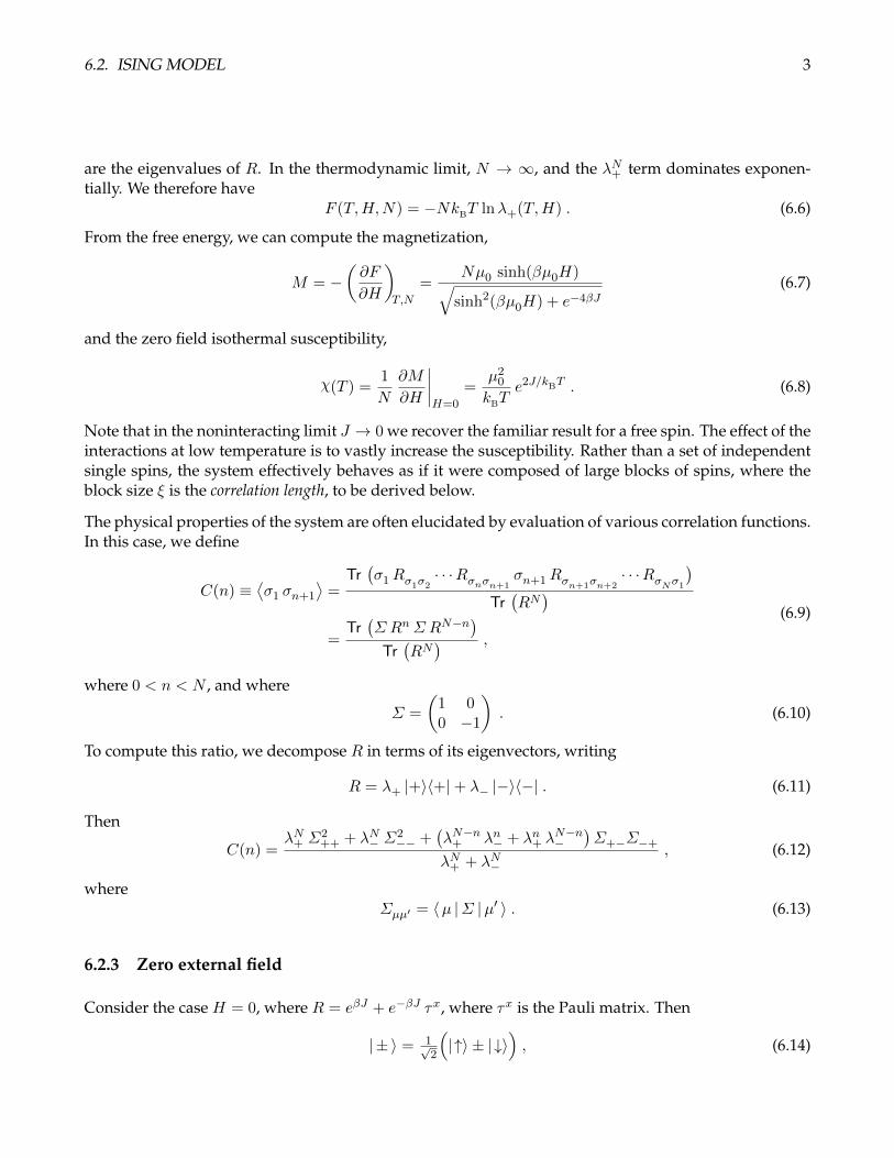
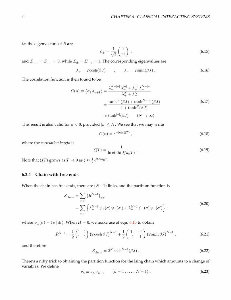

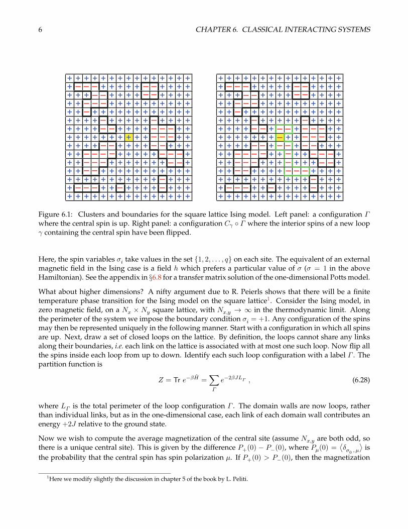
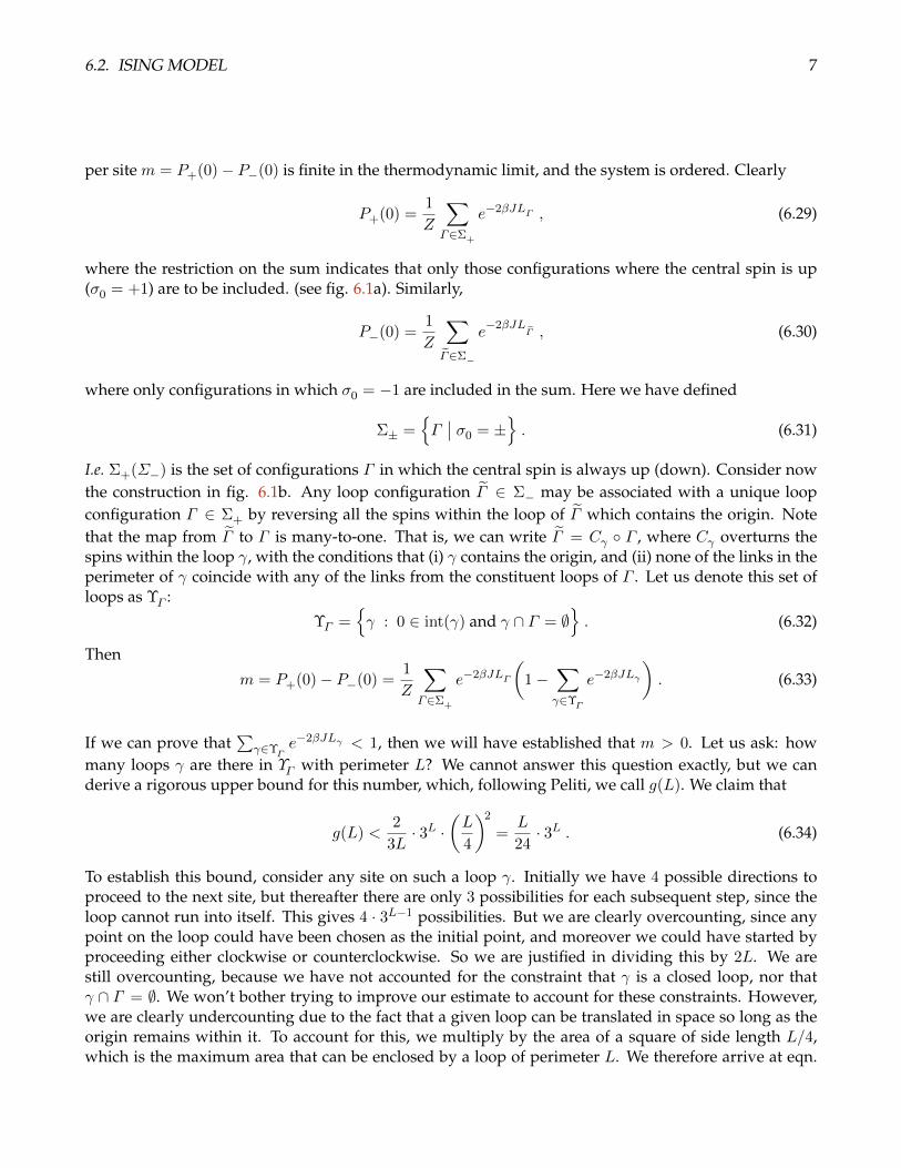


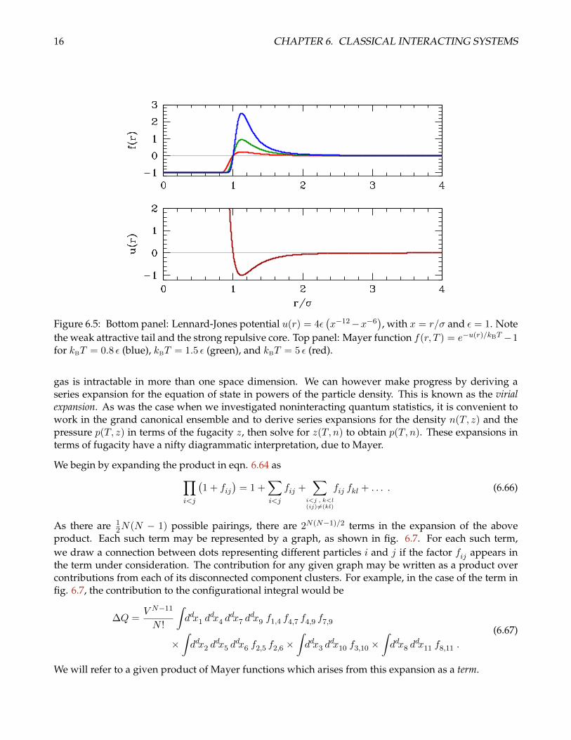
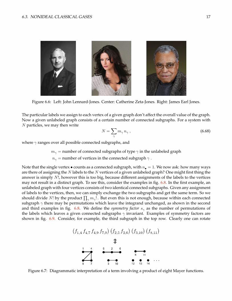


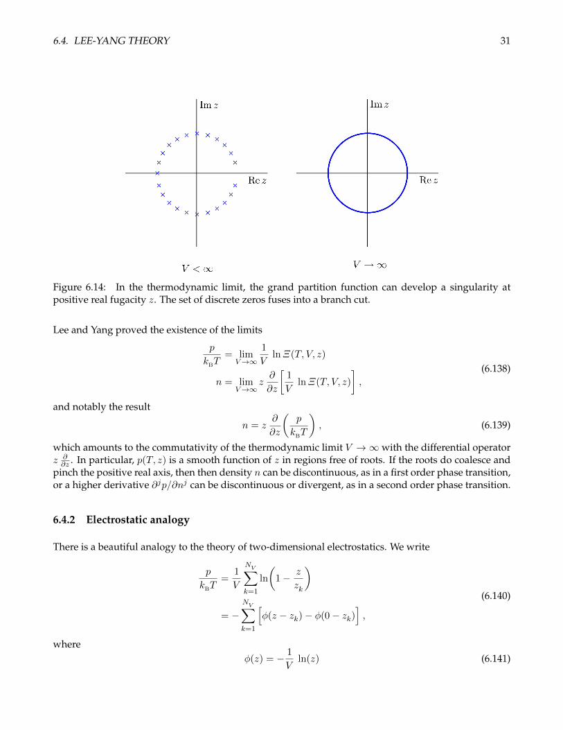


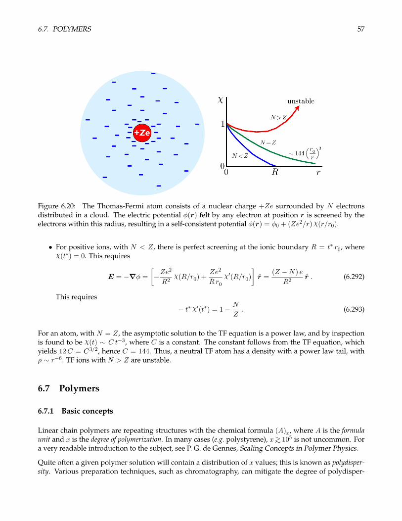

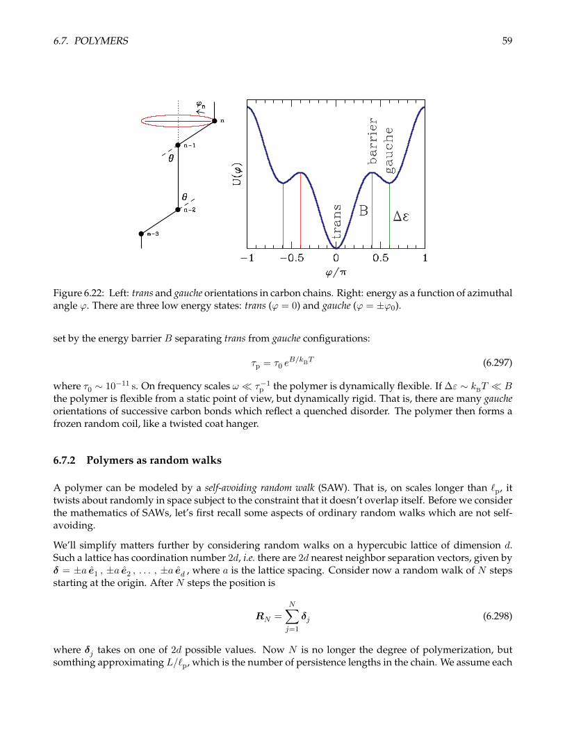
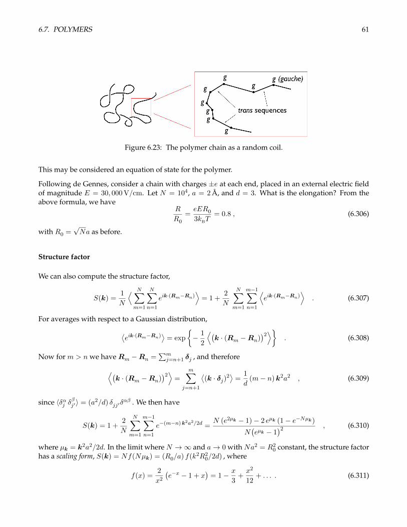


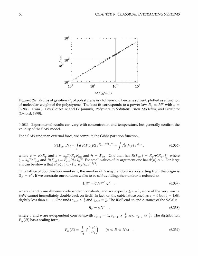


![The threshold criterion of the Gross-Pitaevskii equation with ......Gross-Pitaevskii equation for trapped dipolar quantum gases, nonlinearity 21(2008)2569-2590 [M-W] L.Ma, J.Wang,](https://static.documents.pub/doc/80x56/61026bcfa9e58f0229607679/the-threshold-criterion-of-the-gross-pitaevskii-equation-with-gross-pitaevskii.jpg)


