An EOQ model with variable holding cost and partial backlogging under credit limit policy and cash discount
Mohit Rastogia*, S.R. Singhb, Prashant Kushwaha and Shilpy Tayalb aCentre for Mathematical Sciences, Banasthali University, Banasthali, Rajasthan, India bDepartment of Mathematics, CCS University, Meerut, India
C H R O N I C L E A B S T R A C T
Article history: Received April 2, 2016 Received in revised format June 12, 2016 Accepted August 17 2016 Available online August 18 2016
In this paper we develop an inventory model for deteriorating items with price sensitive demand. Generally the vendor offers a cash discount or fix time period to the retailer to pay all the dues. According to the availability of money the retailer chooses his/her option. In this paper we discuss the possible cases of permissible delay and cash discount. The shortages are allowed in this model and are partially backlogged. Holding cost is considered as varying function of time, which reflects a more realistic concept. The purpose of this study is to optimize the overall cost of the system and to compute optimal ordering quantity. Numerical examples for different cases are also presented to illustrate the study. A sensitivity analysis with regard to distinct associated parameters is shown to make sure the constancy of the model.
In today’s competitive business environment, a vital factor for the success of any business organization is a healthy connection between vendor and buyer. Since both buyer and vendor may endorse the business by creating a relationship between themselves so business environment necessitates an innovative spirit of collaboration between both buyer and vendor. Traditionally while developing models for various inventory systems, mostly researchers assume that the retailer’s funds are enough and must be paied to the supplier as soon as the goods are received. But in real business world, this assumption does not hold. Generally it is very often seen that the supplier offers a scheme of trade credit period to the retailer to settle the account. During the allowable trade credit period no interest is chargeable and after that an interest will be charged on unpaid amount. So, it will be advantageous to disburse later, as it decreases stock’s holding cost, ultimately. This policy works as an incentive policy for the retailer because during this period the retailer can sell the products, accumulate the revenues and receive interest on the capital. On the other hand, this credit policy offers an advantage to the
28
supplier to catch the attention of more customers for increase the sale. Thus, trade credit plays a vital role in inventory management for both the supplier and the retailer. Firstly, Haley and Higgins (1973) presented the model to deem EOQ under permissible delay in payments. In this model they deem demand as constant. Goyal (1985) investigated a single item EOQ model under permissible delay in payments. By incorporating the effect of deterioration, Goyal’s model was extended by Aggarwal and Jaggi (1995). Teng et al. (2005) presented an optimal ordering and pricing policy with allowable trade credit period. Chang et al. (2009) presented an optimal inventory policy for deteriorating items under inflation and permissible delay in payments. Ouyang et al. (2010) proposed a fuzzy inventory model with deterioration by assuming, the credit period linked to order quantity. Singh et al. (2011) presented a deterministic two warehouse inventory model for deteriorating items with stock-dependent demand and shortages under the conditions of permissible delay. Singh and Sharma (2014) studied an optimal policy for trade credit considering imperfect production and demand rate as stock dependent. Tayal et al. (2015) developed a production model for integrated inventory with preservation technology and trade credit period. Shastri et al. (2015) suggested a supply chain management with ramp-type demand and partial backordering under trade credit effect. Demand is a vital part for the development of an inventory model. A distinct kinds of demand, used in the inventory modeling. The frequently known demand patterns are constant, time dependent, stock dependent and selling price dependent. Normally it is seen that the selling price of goods is most affecting factor of demand. Burwell et al. (1997) suggested an economic lot size model for price dependent demand under quantity and freight discounts. Mondal et al. (2003) investigated an inventory system of ameliorating items in which demand rate is price dependent. You and Hsieh (2007) presented an EOQ model in which demand rate is taken as a function of available stock and price. Maiti et al. (2009) presented an inventory model with price-dependent demand for an item in stochastic environment. Chang et al. (2010) introduced inventory models for finding the optimal selling price and order quantity under EOQ model for deteriorating item in which demand depends on the on-display stock level as well as selling price per unit. Tayal et al. (2014) studied a deteriorating inventory model by assuming demand as a function of price and season. Mostly inventory practitioners considered that commodities have infinite life time, but depreciation always occurs in the stock. This depreciation may be in the form of deterioration, damage and breakage. In the present model we have considered that the loss in inventory occurs owing to deterioration. Deteriorating inventory has been extensively addressed in the literature and Raafat (1991) presented a very thorough literature review on applications of deteriorating inventory. According to the study of Goyal and Giri (2001) decaying products, such as volatile liquids, food products, electronic components etc., are associated with an extremely wide range of inventory commodities. Manna and Chaudhary (2006) presented an optimal ordering quantity inventory model with ramp type demand rate, time dependent deterioration rate and allowable shortages. Hsu et al. (2007) developed an inventory model for deteriorating items with expiration date and uncertain lead time. Widyadana et al. (2011) presented an economic order quantity model for deteriorating items and planned backorder level. Shukla et al. (2013) explored a deteriorating model by considering shortages and exponential demand. Singh et al. (2016) introduced an EOQ model by considering demand as stock dependent with trade credit for deteriorating products. The traditional parameters such as holding cost, setup cost and demand rate in classical EOQ models generally are assumed to be fixed. Consequently, classical models have some dissimilarity with real-life situations. This issue has encouraged lots of researchers to amend the EOQ model to match real-world conditions. The assumption, holding cost is always fixed is not true in general and thus to represents real-life situations, in this paper holding cost is assumed to be a varying function of time. This is mainly true for non-instantaneous deteriorating products such as food products during their storage. The longer these items will be held in storage, the more services and the storage amenities will be required that results an increment in the holding cost. In establishing of EOQ models, a variety of
M. Rastogi et al. /Uncertain Supply Chain Management 5 (2017)
29
functions describing holding cost were careful by some researchers like Weiss (1982), Goh (1994) and Roy (2008). Mishra et al. (2013) introduced an inventory model for perishable items with variable holding cost and partial backlogging. In this model demand is considered as time dependent. Tayal et al. (2015) suggested a production quantity model by considering variable holding cost for non-instantaneous deteriorating products. Many articles assume that in the case of stock out all the happening demand will either completely lost/completely backlogged. But, in common the happening demand during stock out is partially backlogged/partially lost. The customers wait up-to the next replenishment to fulfill their demand. The backlogged demand depends on the length of the waiting time. Moreover, the opportunity cost due to lost sales should be careful since a few customers would not like to wait for backlogging during the shortage periods. Chang and Dye (1999) developed an inventory model with time varying demand and partial backlogging. Ouyang et al. (2005) developed an inventory model for deteriorating items with exponential declining demand and partial backlogging. Singh and Singhal (2008) introduced a two warehouse partial backlogging inventory model for perishable products having exponential demand. Singh et al. (2010) developed a volume flexible inventory model for defective items with multivariate demand and partial backlogging. Tayal et al. (2014) introduced a deteriorating model with effective investment in preservation technology. In this model the shortages are allowed and the occurring shortages are partially backlogged. In this study, we attempted to combine all above stated aspects into a solo problem. Entire atmosphere of business connections has been considered, that matchs to realistic market conditions. Generally the vendor offers a cash discount or fix time period to the retailer to pay all the dues. According to the availability of money the retailer chooses his option. In this chapter we have discussed the possible cases of permissible delay and cash discount. Shortages are permitted and happening shortages are backlogged partially. Also assumption of holding cost to be a varying function of time which reflects a more realistic concept, has been taken in to explanation in this study. 2. Assumptions and Notations
Assumptions
In order to develop present model, some specific assumptions used are given below: 1. The products discussed in this model are assumed to be in deteriorating nature.
2. Demand for the products is a function of selling price and follows as .3. Holding cost assumed as a variable function of time and is given by h(t) = ( h1+h2t). 4. Shortages are allowed. 5. The rate of backlogging is a function of waiting time up to the next arrival and is given by θ(η)
= 1− . 6. A permissible delay period is allowed to the retailer to pay all his/her dues, but if he/she does
not pay all the amount at this time, an interest will be charged on the balanced amount. Notations
The following are the notations used throughout this model. K Deterioration parameter α, β Demand parameters p selling price per unit T cycle time v the critical time at which inventory level becomes zero I1(0) initial inventory level for the retailer Q2 backordered quantity during stock out c purchasing cost per unit θ(η) rate of backlogging during stock out
30
η waiting time up to the arrival of next lot h1, h2 holding cost parameters Q initial inventory level d deterioration cost per unit O ordering cost per order s shortage cost per unit l lost sale cost per unit x rate of cash discount Ie rate of interest earned by the buyer Ic rate of interest charged by the vendor T.A.C. Total Average Cost
3. Formulation and Solution of the Model
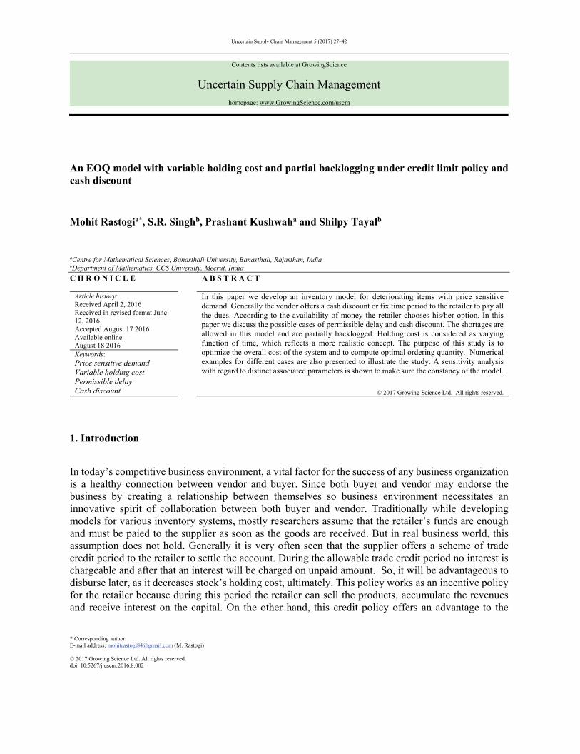
Fig. 1 shows the inventory time behavior of this system. For retailer, I1(0) denotes initial inventory level. The inventory level for the retailer decreases by reason of demand and deterioration effect during [0, v]. Inventory level becomes zero at t=v and afterward shortages take place. The happening shortages are partially backlogged with waiting time dependent rate of backlogging.
Differential equations showing the behavior of inventory with time are as follows:
11
( )( )
dI tKI t
dt p
0 t v
(1)
22
( )( )
dI tKI t
dt p
v t T
(2)
with boundary conditions 1( ) 0I v and 2 ( ) 0I v . With the help of these boundary conditions the
solution of these equations are given as follows:
( )1( ) ( 1)K v tI t e
p K
0 t v
(3)
2 ( ) ( )I t v tp
v t T
(4)
From Eq. (3):
1(0) ( 1)KvI ep K
(5)
Inventory
2Q
(01I(t1I
Time Tv
Fig. 1. Inventory time graph for the retailer
M. Rastogi et al. /Uncertain Supply Chain Management 5 (2017)
shortage cost + lost sale cost + Interest charged – Interest earned]
(6)
Purchasing cost:
1 2. . ( (0) )P C I Q c
where 2 22 ( ) ( )
2
T
v
Q dt T vp p T
2 2. . ( ( 1) ( ))2
KvP C e T v cp K p T
(7)
Holding cost:
21
1 2 1 1 2 2 20
1 1. . ( ) ( ) [ ( )( ) ( )]
2
v KvKvh e v
H C h h t I t dt e h h v v hp K K K K
(8)
Deterioration cost:
1. . { (0) (0, )}D C d I D v
Here 0
(0, )v
D v dtp
(9)
1. . { }
Kvd eD C v
p K
(10)
Ordering cost:
. .O C O
(11)Shortage cost:
. . ( )T
v
sS C s dt T v
p p
(12)
Lost sale cost:
2. . . (1 ( )) ( )2
T
v
lL S C l dt T v
p Tp
(13)
Since a cash discount or permissible delay period is allowed to the retailer by the vendor, then based on these conditions the different cases arise:
Case 1: When a cash discount is offered to the retailer by the vendor
In this case the retailer pays all the payment at the time of arrival of stock, for which the vendor offers a cash discount at a rate of x%. The purchasing cost in this case will be:
2 2. . ( ( 1) ( )) (1 )2 100
Kv xP C e T v c
p K p T
(14)
Interest earned in this case:
32
2
1
0
.2
T
e e
TI E pI t dt pI
p p
(15)
In this case the T.A.C. of the system will be:
2 21 1. . . [( ( 1) ( )) (1 ) { } ( )
2 100
KvKv x d e s
T AC e T v c v O T vT p K p T p K p
2 2
211 2 2 2
1 1{ ( )( ) ( )} ( ) ]
2 2 2
KvKv
e
h e v l Te h h v v h T v pI
p K K K K Tp p
(16)
Case 2: When a permissible delay period is allowed to the retailer
In this case the supplier offers a period of M units to the retailer to pay all the dues. Now based on this credit time limit two conditions arise:
Case (2.1): When permissible delay period (M) is greater than the critical time ( M v )
Case (2.2) : When permissible delay period (M) is less than the critical time ( M v )
Case 2: When a permissible delay period is allowed to the retailer
In this case the supplier offers a period of M units to the retailer to pay all the dues. Now based on this credit time limit two conditions arise:
Case (2.1): When permissible delay period (M) is greater than the critical time ( M v )
Case (2.2): When permissible delay period (M) is less than the critical time ( M v )
Case (2.1): When permissible delay period (M) is greater than the critical time ( M v )
In this case the permissible delay period (M) is greater than the critical time as shown in Fig.2, and so the total available money at the time of payment will be greater than the total required amount. Thus the interest charged in his case will be zero.
2
2.1
0 0
. { ( ) } { ( ) }2
v v
e e
vI E pI t dt M v dt pI M v v
p p p p
(17)
2.1. 0I C (18)
T.A.C. of the system in this case will be:
Inventory
0 Mv Time
Fig. 2. When M v
M. Rastogi et al. /Uncertain Supply Chain Management 5 (2017)
33
2 22.1
1 1. . [( ( 1) ( )) { } ( )
2
KvKv d e s
T AC e T v c v O T vT p K p T p K p
2
211 2 2 2
1 1{ ( )( ) ( )} ( )
2 2
KvKvh e v l
e h h v v h T vp K K K K Tp
2
{ ( ) }]2e
vpI M v v
p p
(19)
Case (2.2): When permissible delay period (M) is less than the critical time ( M v )
In this case the permissible delay period (M) is less than the critical time as shown in Fig.3. Now based on the total available capital at the time of payment two different cases arise:
(2.2.1) When 2[0, ] [0, ]p D M IE M cQ
(2.2.2) When 2[0, ] [0, ]p D M IE M cQ
Case (2.2.1): When 2[0, ] [0, ]p D M IE M cQ
In this case the retailer has enough money to pay all the dues at t=M,
Interest earned in this case
22 2
2
0
. { } ( )2 2
M v
e e e
M
MI E pI t dt tdt pI pI v M
p p p p
(20)
2.2.1. 0I C (21)
T.A.C. of the system in this case will be:
2 22.2.1
1 1. . [( ( 1) ( )) { } ( )
2
KvKv d e s
T AC e T v c v O T vT p K p T p K p
2
211 2 2 2
1 1{ ( )( ) ( )} ( ) }
2 2
KvKvh e v l
e h h v v h T vp K K K K Tp
2
2 2( )]2 2e e
MpI pI v M
p p
(22)
Case (2.2.2): When 2[0, ] [0, ]p D M IE M cQ
In this case the available money to the retailer is not enough to pay all the dues. So an interest will be charged on the balance or unpaid amount.
v M0 Time
Inventory
Fig. 3. When M v
34
Unpaid amount (B)= 1 2(0) { [0, ] . [0, ]}cI pD M I E M (23)
where M
0
D(0,M)=p p
dt M
(24)
Interest charged in this case will be:
2
2.2.2. ( ) { ( )}( )2c e c
p MI C B v M I cQ M pI v M I
p p
(25)
T.A.C. of the system in this case will be:
2 22.2.2
1 1. . [( ( 1) ( )) { } ( )
2
KvKv d e s
T AC e T v c v O T vT p K p T p K p
2
211 2 2 2
1 1{ ( )( ) ( )} ( ) }
2 2
KvKvh e v l
e h h v v h T vp K K K K Tp
2 2
2 2{ ( )}( ) ( )]2 2 2e c e e
p M McQ M pI v M I pI pI v M
p p p p
(26)
4. Numerical Example
Case 1: When a cash discount is offered to the retailer by the vendor
25 / , 14 / , 35 , 500, 1.5, 0.05, 14 / ,ep Rs unit c rs unit T days I d Rs unit
1 25 / , 6 / , 0.001, 0.5 / , 0.05 / , 2s Rs unit l Rs unit K h Rs unit h Rs unit x days
500 /O Rs order
Corresponding to these input values, optimal value of v and T.A.C. come out to be: 34.1795v days and . . . 59.8285T AC Rs respectively. The below mentioned Fig.4 shows that the
model is convex in this case.
Fig. 4. Convexity of the T.A.C. (case 1) Fig. 5. Convexity of the T.A.C. (case 2.1)
Case (2.1): When a permissible delay period is allowed to the retailer and M v
25 / , 14 / , 35 , 500, 1.5, 0.05, 14 / ,ep Rs unit c rs unit T days I d Rs unit
1020
3040
50
200
400
600
800
1000
60
65
70
75
1020
3040
10
20
30
40
2000
4000
6000
8000
10000
2040
6080
10
20
30
M. Rastogi et al. /Uncertain Supply Chain Management 5 (2017)
35
1 25 / , 6 / , 0.001, 0.5 / , 0.05 / , 35s Rs unit l Rs unit K h Rs unit h Rs unit M days
500 /O Rs order Based on the input values, optimal value of v and T.A.C. come out to be:
19.8665v days and . . . 17.293T A C Rs respectively. The below mentioned Fig.5 shows that the model is convex in this case.
Case (2.2): When a permissible delay period is allowed to the retailer and M v
(2.2.1): 2[0, ] [0, ]p D M IE M cQ
25 / , 14 / , 35 , 500, 1.5, 0.05, 14 / ,ep Rs unit c rs unit T days I d Rs unit
1 25 / , 6 / , 0.001, 0.5 / , 0.05 / , 15s Rs unit l Rs unit K h Rs unit h Rs unit M days
500 /O Rs order Based on the input values, optimal value of v and T.A.C. come out to be:
34.1587v days and . . . 60.9669T A C Rs respectively. The below mentioned Fig.6 shows that the model is convex in this case.
Fig. 6. Convexity of the T.A.C. (case 2.2.1) Fig. 7. Convexity of the T.A.C. (case 2.2.2)
(2.2.2): 2[0, ] [0, ]p D M IE M cQ
25 / , 14 / , 35 , 500, 1.5, 0.05, 14 / ,ep Rs unit c Rs unit T days I d Rs unit
1 25 / , 6 / , 0.001, 0.5 / , 0.05 / , 15s Rs unit l Rs unit K h Rs unit h Rs unit M days
0.07, 500 /cI O Rs order Corresponding to these input values, optimal value of v & T.A.C. found to be:
24.3228v days and . . . 63.8816T A C Rs respectively. Fig.5.7 shows that the model is also convex in this case.
5. Sensitivity Analysis
Sensitivity analysis in respect of distinct associated parameters is performed. We have discussed this analysis only for two cases.
Case 1: When M v
Table 1 Effect on optimal solution for distinct values of selling price (p)
% change in p p v T.A.C. % change p v T.A.C.-20% 20 18.1929 40.3804 5% 26.25 20.2268 13.3365-15% 21.25 18.6511 33.2121 10% 27.5 20.5682 9.87606-10% 22.5 19.0809 27.0963 15% 28.75 20.8922 6.83546-5% 23.75 19.4852 21.8401 20% 30 21.2002 4.152620% 25 19.8665 17.293
1020
3040
50
10000
20000
30000
65
70
75
1020
3040
10
20
30
40
20
40
60
80
100
60
80
100
10
20
30
36
Fig. 8. Variation in total average cost w.r.t. selling price (p)
Fig. 9. Variation in total average cost w.r.t. parameter (α)
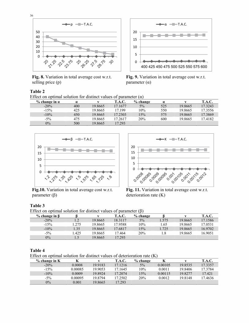
Table 2 Effect on optimal solution for distinct values of parameter (α)
From the above discussion we have observed the following points.
1. Table 1 and Table 7 show that an increment in selling price (p) the overall system average cost decreases and it is highly sensitive with respect to the selling price. This effect can be observed by the Fig.8 & Fig.14 also.
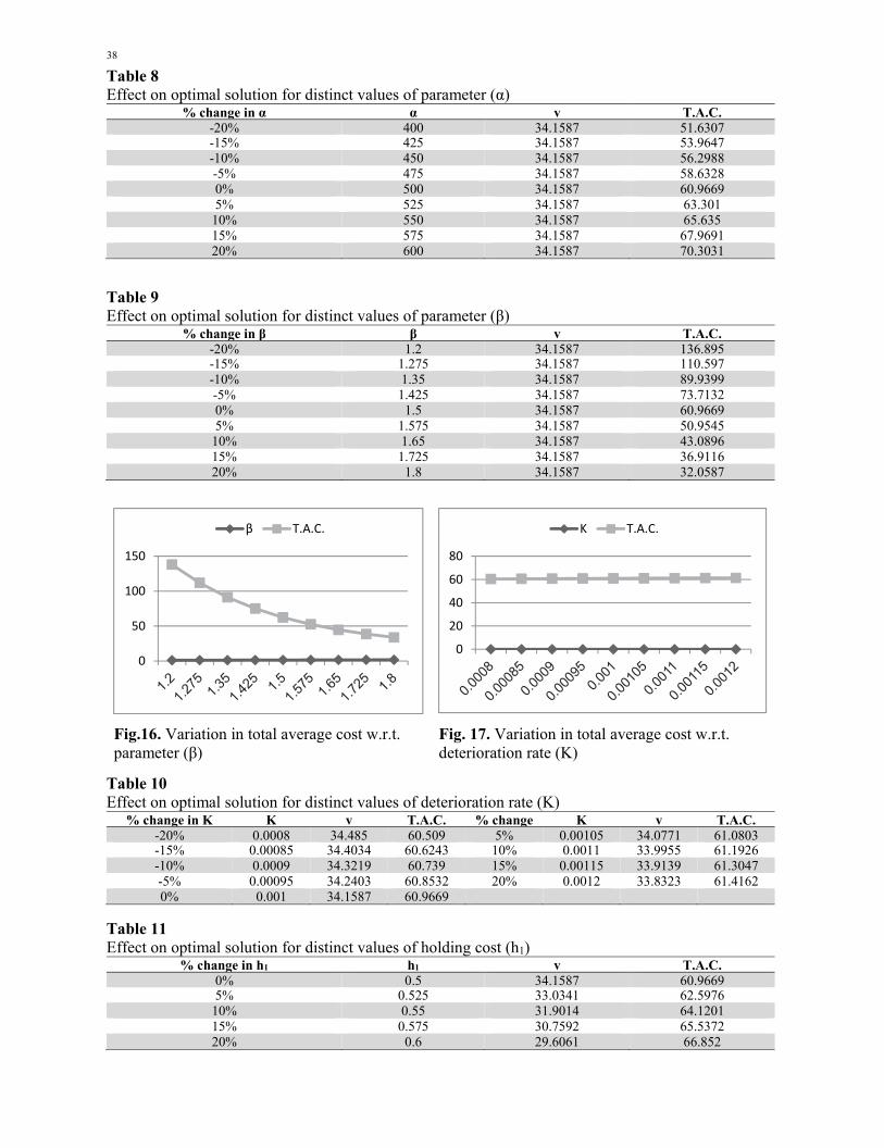
2. Table 2 and table 8 present the effect of demand parameter (α) on v and T.A.C. It is noticed from these tables that with an increment in demand parameter (α), T.A.C. of the system slightly increase. This effect can be observed by the Fig.9 & Fig.15 also.
3. Table 3 and table 9 list variation of demand parameter (β) at dissimilar points and remaining variable unaltered. From this it is noticed that as parameter (β) increase, value of T.A.C. decreases. This effect can be observed by the Fig.10 & Fig.16 also.
4. Table 4 and Table 10 put forward the variation in deterioration parameter (K) by -20%, -15%,-10%, -5%, 0, 5%, 10%, 15%, 20% and from these we examine that with the increment in K, value of T.A.C. slightly increases. This effect can be observed by the Fig.11 & Fig.17 also.
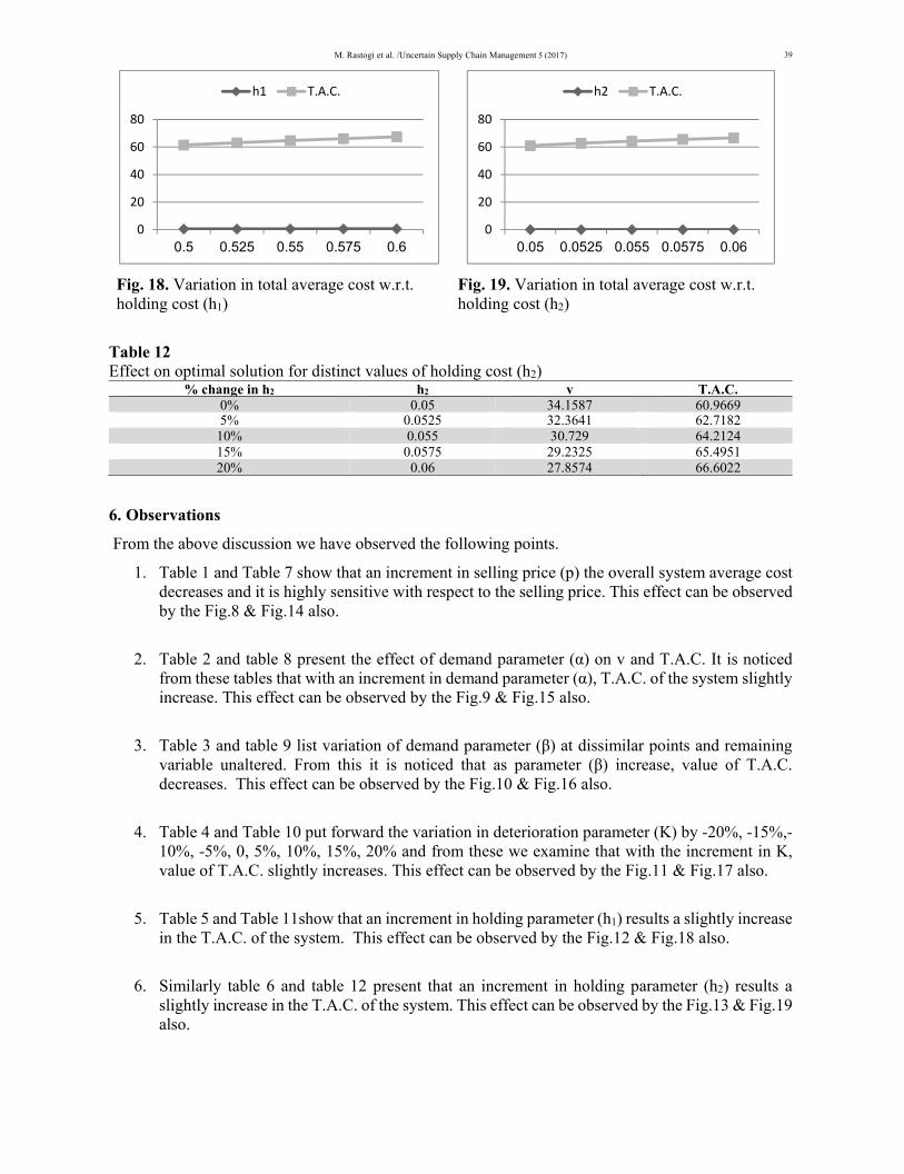
5. Table 5 and Table 11show that an increment in holding parameter (h1) results a slightly increase in the T.A.C. of the system. This effect can be observed by the Fig.12 & Fig.18 also.
6. Similarly table 6 and table 12 present that an increment in holding parameter (h2) results a slightly increase in the T.A.C. of the system. This effect can be observed by the Fig.13 & Fig.19 also.
0
20
40
60
80
0.5 0.525 0.55 0.575 0.6
h1 T.A.C.
0
20
40
60
80
0.05 0.0525 0.055 0.0575 0.06
h2 T.A.C.
40
7. Conclusion
The present paper concern with the real-life business necessities.In this model, we have presented a model for deteriorating products with the conditions of cash discount and permissible delay. It is observed that the vendor generally offers a cash discount to release the payment early. In this study, the possible cases of permissible delay are discussed which make the study very beneficial. From this model it is concluded that to follow the permissible delay period is beneficial for the retailer if this allowable period is greater than the critical time(i.e. time at which inventory is zero). But if the allowable trade credit period is small than the critical point than to pay the purchasing cost with cash discount will be beneficial for the retailer. To make the study close to reality holding cost assumed as variable function, which increases with time. A permissible delay period allowed by the supplier is an incentive scheme to the retailer by which the total inventory cost of the system can be reduced is a vital output of this paper. Numerical examples of different cases and sensitivity analysis with regard to distinct associated parameters are also presented to demonstrate our study. For the future research point of view the model discussed here may be extended in various ways such as for seasonal items, multi items and for time value of money.
Acknowledgement
The authors would like to thank the annonymous referees for constructive comments on earlier version of this paper.
References
Aggarwal, S.P., & Jaggi, C.K. (1995). Ordering Policies of Deteriorating Item Under Permissible Delay in Payments. Journal of the Operational Research Society, 46(5), 658–662.
Burwell T.H., Dave D.S., Fitzpatrick K.E., & Roy, M.R. (1997). Economic lot size model for price-dependent demand under quantity and freight discounts. International Journal of Production Economics, 48(2), 141-155.
Chang, C.T., Chen, Y.J., Tsai, T.R., & Wu, S.J. (2010).Inventory models with stock-and price dependent demand for deteriorating items based on limited shelf space. Yugoslav Journal of Operations Research, 20(1), 55-69.
Chang, C-T., Wu, S-J., & Chen, L-C. (2009). Optimal payment time with deteriorating items under inflation and permissible delay in payments. International Journal of System Science, 40, 985-993.
Chang, H. J., & Dye, C. Y. (1999). An EOQ model for deteriorating items with time varying demand and partial backlogging”, Journal of Operational Research Society, 50(11), 176-1182.
Goh, M. (1994). EOQ models with general demand and holding cost functions. European Journal of Operational Research, 73(1), 50-54.
Goyal, S.K. (1985). Economic ordering quantity under conditions of permissible delay in payments. Journal of the Operational Research Society, 36(4), 335–343.
Goyal, S.K., & Giri, B.C. (2001). Recent trends in modeling of deteriorating inventory. European Journal of Operational Research, 134(1), 1–16.
Hsu, P. H., Wee, H. M., & Teng, H. M. (2007). Optimal ordering decision for deteriorating items with expiration date and uncertain lead time. Computers & Industrial Engineering, 52(4), 448–458.
Maiti, A., Mait, M., & Maiti, M. (2009). Inventory model with stochastic lead-time and price dependent demand in corporating advance payment. Applied Mathematical Modelling, 33(5), 2433-2443.
Manna, S.K., & Chaudhuri, K.S. (2006). An EOQ model with ramp type demand rate, time dependent deterioration rate, unit production cost and shortages. European Journal of Operation Research, 171(2), 557–566.
M. Rastogi et al. /Uncertain Supply Chain Management 5 (2017)
41
Mishra, V. K., Singh, L. S., & Kumar, R. ( 2013). An inventory model for deteriorating items with time-dependent demand and time-varying holding cost under partial backlogging. International Journal of Industrial Engineering, 9(4), 267-271.
Mondal, B., Bhunia, A.K., & Maiti, M. (2003). An inventory system of ameliorating items for price dependent demand rate. Computers and Industrial Engineering, 45(3), 443-456.
Ouyang, L.Y., Teng, J.T., & Cheng, M.C. (2010). A fuzzy inventory system with deteriorating items under supplier credits linked to ordering quantity. Journal of Information Science and Engineering, 26(1), 231–254.
Ouyang, L.Y., Wu, K. S. and Cheng, M. C. (2005).An inventory model for deteriorating items with exponential declining demand and partial backlogging. Yugoslav Journal of Operations Research, 15(2), 277-288.
Raafat, F. (1991). Survey of Literature on Continuously Deteriorating Inventory Models. Journal of the Operational Research Society, 42(1), 27–37.
Roy, A. (2008). An inventory model for deteriorating items with price dependent demand and time varying holding cost. Advanced Modeling and Optimization, 10(1), 25–37.
Shastri, A., Singh, S. R., & Gupta, S. (2015). Supply chain management under the effect of trade credit for deteriorating items with ramp-type demand and partial backordering under inflationary environment. Uncertain Supply Chain Management, 3(4), 339–362.
Shukla, H. S., Shukla, V., & Yadav, S. K. (2013). EOQ model for deteriorating items with exponential demand rate and shortages. Uncertain Supply Chain Management, 1(2), 67-76.
Singh, S. R., Khurana , D., & Tayal, S. (2016). An economic order quantity model for deteriorating products having stock dependent demand with trade credit period and preservation technology. Uncertain Supply Chain Management, 4(1), 29-42.
Singh S. R., Kumari, R., & Kumar, N. (2011). A deterministic two warehouse inventory model for deteriorating items with stock-dependent demand and shortages under the conditions of permissible delay. International Journal of Mathematical Modelling and Numerical Optimization, 2(4), 357-375.
Singh, S.R., & Sharma, S. (2014). Optimal trade credit policy for perishable items deeming imperfect production and stock dependent demand. International Journal of Industrial Engineering Computations, 5(1), 151-168.
Singh, S. R., & Singh, S. (2008). Two warehouse partial backlogging inventory model for perishable products having exponential demand. International Journal of Mathematical Sciences and Computer, 1(1), 229-236.
Singh, S. R., Singhal, S., & Gupta, P. K. (2010). A volume flexible inventory model for Defective Items with multi variate demand and partial backlogging. International Journal of Operations Research and Optimization, 1(4), 54-68.
Tayal, S., Singh, S. R., & Sharma, R. (2014). An inventory model for deteriorating items with seasonal products and an option of an alternative market. Uncertain Supply Chain Management, 3(1), 69–86.
Tayal, S., Singh, S. R., & Sharma, R. (2015). An integrated production inventory model for perishable products with trade credit period and investment in preservation technology. International Journal of Mathematics in Operational Research, Article ID 76334.
Tayal, S., Singh, S. R., Sharma, R., & Chauhan, A. (2014). Two echelon supply chain model for deteriorating items with effective investment in preservation technology. International Journal Mathematics in Operational Research, 6(1), 78-99.
Tayal, S., Singh, S. R., Sharma, R., & Singh A. P. (2015). An EPQ model for non-instantaneous deteriorating item with time dependent holding cost and exponential demand rate. International Journal of Operational Research, 23(2), 145-161.
Teng, J. T., Chang, C. T., & Goyal, S. K. (2005). Optimal pricing and ordering policy under permissible delay in payments. International Journal of Production Economics, 97(2), 121-129.
Widyadana, G. A., Cárdenas-Barrón, L. E., & Wee, H. M. (2011). Economic order quantity model for deteriorating items with planned backorder level.Mathematical and Computer Modelling, 54(5), 1569-1575.
42
Weiss, H. J. (1982). Economic order quantity models with nonlinear holding costs. European Journal of Operational Research, 9(1), 56-60.
You, P. S., & Hsieh, Y. C. (2007). An EOQ model with stock and price sensitive demand. Mathematical and Computer Modelling, 45(7), 933-942.