Contesting an International Trade Agreement∗

Matthew T. Cole†, California Polytechnic State University

James Lake‡, Southern Methodist University

Ben Zissimos§, University of Exeter Business School

June 19, 2017

Abstract

After governments sign an international trade agreement (TA), each government must

ratify the TA. Often, this ratification process is lengthy and the outcome highly uncer-

tain. We model a two-country TA where, unlike prior literature, pro-trade and anti-

trade interest groups in each country recognize that (i) TA implementation requires

ratification by both governments and (ii) they cannot condition contributions on their

government’s ratification decision. In this new class of contests, which we call ‘parallel

contests’, we show that (i) anti- and pro-trade lobbies lobby in equilibrium, (ii) the

probability of TA ratification lends itself to intuitive and tractable comparative statics,

and (iii) the protection embodied in negotiated TA tariffs reflects a tension between

the liberalizing force of lobbying and inherently protectionist government preferences.

∗For useful comments and conversations about earlier drafts we thank Toke Aidt, Scott Baier, RickBond, Axel Dreher, Giovanni Facchini, Philipp Harms, Carsten Hefeker, Arye Hillman, Benjamin Ho, DanKovenock, Emanuel Ornelas, Alejandro Riano, Ray Riezman, Joel Rodrigue, Kamal Saggi and Tim Salmon,as well as seminar and conference participants at Cal Poly, ETH Zurich, Florida International University,Georgia Tech, Kings College London, London School of Economics, Indiana University, Southern MethodistUniversity, University of Exeter, University of Nottingham, European Trade Study Group meeting, INFERworkshop, Silvaplana Workshop in Political Economy, KU Lueven Workshop on International Trade Agree-ments, SAET conference, UECE Lisbon Meetings in Game Theory and Applications, Southern EconomicsAssociation conference, Midwest Trade meetings, InsTED conference.†Department of Economics, California Polytechnic State University, CA 93407, USA. Email: mt-

cole@calpoly.edu.‡Department of Economics, Southern Methodist University, Dallas, TX 75275, USA. Email:

jlake@smu.edu§Corresponding author: Department of Economics, University of Exeter Business School, Streatham Cam-

pus, Exeter EX4 4ST, UK. Email: b.zissimos@exeter.ac.uk.

1 Introduction

Anecdotal evidence suggests conflicting lobbying interests and inherent ratification uncer-

tainty characterize international trade agreements (TAs). Despite the final text of the

Uruguay Round of multilateral negotiations being essentially settled in December 1993, it was

not signed until April 1994 and not ratified by the US Congress until December 1994.1 With

about 12 months between completion of negotiations and ratification, Strange (2013, p.121)

documents the conflicting lobbying interests between US small businesses, represented by the

anti-trade ‘US Business and Industrial Council’, and major US corporations, represented by

the pro-trade ‘Alliance for GATT Now’ (also, see Dam (2001, p.14)). Even after the affir-

mative US House of Representatives vote on November 29th 1994, media reports explicitly

documented the uncertain outcome in the Senate citing statements by Senate leaders and

last-minute cajoling of wavering Senators by President Clinton.2 Thus, conflicting lobbying

interests and inherent ratification uncertainty have long characterized multilateral TAs.

Multilateral TAs are the historical cornerstone of the TA landscape with countries ne-

gotiating the level of non-discriminatory MFN tariffs. But, TAs between small groups of

countries, the Trans-Pacific Partnership (TPP) among 12 countries being a larger exam-

ple, have proliferated since the Uruguay Round. Known as Preferential Trade Agreements

(PTAs) or Free Trade Agreements (FTAs) because members exchange (essentially) reciprocal

tariff free access while maintaining tariffs on non-members, negotiations center around dura-

tion of product-specific tariff phase-out periods and other non-tariff rules.3 Like multilateral

TAs, substantial time elapses between the start of negotiations and implementation with

the literature suggesting 3-4 years and around half this time for negotiations.4 Again, anec-

dotal evidence suggests conflicting lobbying interests and inherent ratification uncertainty

characterize PTAs.

After release of the final text in October 2015, the TPP provides a recent example span-

ning North American and Asian-Pacific countries. With increased export market access,

various US agricultural groups (e.g. National Pork Producers Council, National Chicken

Council, National Council of Farmer Cooperatives, American Farm Bureau and the Na-

tional Corn Growers Association) and dairy producers (e.g. Land O’Lakes, Kraft-Heinz

1See https://www.wto.org/english/thewto_e/whatis_e/tif_e/fact5_e.htm.2See https://goo.gl/IZ9iTl.3Articulated in GATT Article I, non-discrimintion is the fundamental principle of global trade whereby

a country’s MFN (Most Favored Nation) tariff is imposed on all other countries. The main exception to thisnon-discrimination principle are FTAs, allowed by GATT Article XXIV. GATT Article XXIV only requiresFTA members eliminate trade barriers on substantially all trade within a reasonable period of time. Despitethis inherently vague language, Hakobyan et al. (2017) document that excluding products from eventuallybeing tariff free is extremely rare for FTAs involving the US, EU or Japan.

4See Molders (2012, 2015) and Freund and McDaniel (2016).

1

and the National Milk Producers Federation) lobbied in support of the TPP. Further lobby

support came from those also benefiting from tariff free intermediate inputs (e.g. Nike, Wal-

mart and the Outdoor Industry Association). Lobby group opposition in the US came from

automakers (e.g. Ford and General Motors), based on the TPP not addressing currency

manipulation issues, tobacco manufacturers (e.g. Phillip Morris and Altria), because the

TPP excluded the tobacco industry from investor-state dispute settlement mechanisms, la-

bor unions (e.g. AFL-CIO, Teamsters and United Steelworkers) and environmental groups

(e.g. Sierra Club). Against this backdrop of conflicting lobbying influences, the Trump ad-

ministration abandoned the TPP in early 2017 despite earlier news reports optimistic over

passage during the Obama-Trump transition period.5

We model a two-country TA where governments negotiate reciprocal liberalization from

initial ‘status quo’ tariffs and interest groups lobby their national government over TA ratifi-

cation. We take these status quo tariffs as exogenous, remaining agnostic about their origin.

Following earlier literature (e.g. Bagwell and Staiger (1999)), our negotiated TA tariffs must

respect a ‘reciprocity rule’ that ensures equal exchange of market access. The only additional

structure imposed on the negotiation process between governments is that it yields a Pareto

efficient outcome. Through modeling negotiated and non-discriminatory MFN tariffs, this

setup represents a multilateral TA. However, PTAs can be thought of as a special case in our

framework where the ‘negotiated’ TA tariffs are exogenously zero rather than endogenous.

Thus, our framework can address either multilateral TAs or PTAs.

Upon negotiation of the TA tariffs, a ‘pro-trade’ and an ‘anti-trade’ lobby make contri-

butions to their national government supporting or opposing the TA. After receiving con-

tributions, each national government decides whether to ‘ratify’ the TA with the negotiated

TA tariffs being implemented only if both governments ratify the TA; otherwise, the status

quo tariffs prevail. Following the contest literature, we model each government’s ratification

decision using a contest success function (CSF); the CSF attaches higher probability to TA

ratification as relative contributions of the pro-trade lobby rise.6

Our framework is quite general. On the political economy side, we consider the possibility

that government TA ratification decisions could depend solely on lobbying contributions or

that ‘additional factors’ may also matter; e.g., national welfare, tariff revenue or employment

5Ratification uncertainty is not a characteristic particular to the TPP. The US House of Representativesvote on CAFTA-DR, a PTA between the US and Central America, lay on a knife edge before eventuallypassing by only two votes. Despite being signed in 2007, similar votes for individual US PTAs with Korea,Colombia and Panama appeared dead before resuscitation by the Obama administration in 2010 and eventualCongressional passage in 2011.

6The contest literature, or ‘Tullock contest’ literature, starts with Tullock (1980) (see Van Long (2013)for a literature review). Skaperdas (1996) axiomatizes the basic CSF where contestants can only make onetype of investment (‘contribution’ in our terminology).

2

in the import-competing sector. These additional factors combine with lobbying contribu-

tions to form an ‘augmented’ contribution.7 On the international trade side, choosing a

particular model of international trade microfounds the strength of lobby support and oppo-

sition for the TA as well as any ‘additional factors’ that influence government TA ratification

decisions. We show how our framework lends itself to various well known models including

the specific factors model, the oligopoly model, and the Melitz model.

Two immediate results emerge in this general setup. First, the anti-trade and pro-

trade lobby groups both make contributions in equilibrium. That is, conditional on the

TA tariffs announced by governments, anti-trade and pro-trade lobbies directly influence

the subsequent equilibrium ratification decision of their own government. As described

above, conflicting lobbying interests are a pervasive feature of the real world TA ratification

process. Nevertheless, in the benchmark “Protection for Sale” lobbying model, only the anti-

trade lobby or the pro-trade lobby makes equilibrium contributions when lobbying over TA

ratification.8 Thus, equilibrium lobbying over TA ratification by the anti-trade and pro-trade

lobbies is an important feature of our framework.

Second, we show that the probability of a government ratifying the TA depends on the

strength of pro-trade lobby support relative to the strength of anti-trade lobby opposition.

Thus, uncertainty always characterizes the TA ratification process and in an intuitive man-

ner. Not only do real world TA ratification processes appear subject to inherent uncertainty,

as described above, but the benchmark Protection for Sale framework predicts that either

TA ratification takes place or that TA ratification does not take place.9 Further, given one

can microfound the strength of support and opposition using a particular underlying model

of trade, our framework allows tractable comparative statics regarding the likelihood of TA

formation. In turn, our framework can shed light on the empirical determinants of PTAs pi-

oneered by Baier and Bergstrand (2004). Section 5 illustrates these features using the Melitz

model, already a cornerstone of the modern empirical and quantitative trade literature.

In addition to results regarding the TA ratification process, our framework also delivers

predictions regarding the TA tariffs negotiated by governments. However, given the general-

7In the Appendix, we show our results are robust to an ‘all-pay contest’ setting where the lobby groupmaking the highest contribution sways their government’s TA ratification decision with certainty. Despitecertainty over the government TA ratification decisions conditional on contributions, all-pay contests havethe well known feature that equilibrium contribution strategies take the form of mixed strategies. Thus,ex-ante, TA ratification decisions remain uncertain.

8See Grossman and Helpman (1995a, p.671). Note, Grossman and Helpman (1994) is the seminalProtection For Sale paper where a single small country unilaterally determines its MFN tariff. Grossmanand Helpman (1995b) extends their traditional setting to multilateral negotiation of MFN tariffs by two largecountries. Grossman and Helpman (1995a) extends their traditional setting to bilateral PTA ratification.

9See Definitions 1-2 of Grossman and Helpman (1995a, p.673, p.676), remembering that each lobby grouplobbies either for or against the TA (Grossman and Helpman (1995a, p.671)).

3

ity of the framework described so far, characterizing the TA tariffs requires further structure

governing the impact of trade liberalization on the strength of interest group support and

opposition for the TA. Specifically, our results use two properties. First, a more liberal TA

polarizes the pro-trade and anti-trade lobby by strengthening the pro-trade lobby’s support

for the TA and strengthening the anti-trade lobby’s opposition to the TA. Second, a more

liberal TA generates pro-trade biased polarization by strengthening the pro-trade lobby’s

support for the TA relative to the anti-trade lobby’s opposition to the TA. In Section 5, we

show these two properties hold quite naturally in a variety of standard trade models.

Numerous insights emerge regarding the TA tariffs negotiated by governments. First,

once lobbying influences have sufficient sway over government TA ratification decisions, the

most liberal TA possible (i.e. subject to the rule of reciprocity discussed above) is the equi-

librium TA. Here, the most liberal TA possible maximizes lobbying contributions, which

dominate a government’s TA ratification decision, by maximizing both the strength of sup-

port and opposition to the TA. This contrasts with typical Protection for Sale setups where

protection rises as government decisions increasingly reflect lobbying influences.

Second, given the most liberal TA possible results when lobbying sufficiently sways gov-

ernment TA ratification decisions, our framework suggests that observed real world protec-

tion levels stem from governments having inherently protectionist preferences (i.e. ‘anti-

trade’ additional factors) which balance the liberalizing influence of lobbying. This contrasts

with the common theme in the Protection for Sale literature where equilibrium protection

results from the balance between protectionist lobbying forces and a national welfare minded

government. Nevertheless, Conconi et al. (2014) present compelling empirical evidence that

governments, and politicians, have inherent protectionist motives related to re-election mo-

tives. Further, Lake and Millimet (2016) show how the PTA voting behavior of US House

Representatives become less protectionist as their constituents receive more trade related

redistribution, especially when the representative faces non-trivial re-election risk.

Third, this contrast between protection emerging from inherently protectionist govern-

ment preferences (our framework) versus protection emerging despite inherently welfare-

minded government preferences (the traditional framework) has implications for using data

to infer the extent to which governments value factors other than lobbying. The empiri-

cal Protection For Sale literature where governments inherently value national welfare has

shown that relatively low real world tariffs imply strongly welfare minded governments (see,

e.g., Goldberg and Maggi (1999) and Gawande and Bandyopadhyay (2000)). Yet, the lit-

erature has often acknowledged that “[t]his finding sits poorly with casual observations”

(Gawande et al. (2012, p116)) of anecdotal evidence regarding the pervasiveness of lobbying.

Our framework offers the perspective that real world tariffs stem from inherent government

4

preferences for protection and, in turn, relatively low tariffs suggest government negotiations

over TA tariffs reflect strong lobbying influences.

The different timing assumption regarding government-lobby interaction explains why

our results differ from the benchmark Protection for Sale framework. In our contest frame-

work, lobbies contribute before their government’s trade policy decision. However, in the

menu auction setting of Protection for Sale, lobbies contribute after their government’s

trade policy decision. This explains why both lobbies contribute in equilibrium and, in

turn, why residual uncertainty prevails over TA ratification. It also explains the different

degrees of liberalization across the frameworks. Because a more liberal TA increases the

strength of anti-trade lobby opposition, a more liberal TA increases (decreases) anti-trade

lobby contributions when they contribute before (after) the government’s trade policy de-

cision. Combined with a more liberal TA increasing pro-trade lobby contributions in both

frameworks, greater liberalization prevails in our contest framework. Indeed, our timing

assumption reflects the reality of trade policy in many national legislatures, including the

US Congress, where lobby groups legally lobby between signing and ratification of a TA but

cannot legally link lobbying contributions to future policy outcomes.10

In Section 5, we explicitly compare our contest framework with the benchmark menu

auction Protection for Sale framework using a variety of underlying trade models, including a

version of the stylized specific factors model from Grossman and Helpman (1995a). Grossman

and Helpman (1995b) show that the status quo tariffs in a two-country world combine

a politics component and a terms of trade component. Further, the TA eliminates the

terms of trade component but leaves the politics component. In contrast, we show that,

when lobbying contributions dominate government ratification decisions among symmetric

governments, our contest framework delivers free trade as the equilibrium TA. Extending this

simple economic environment to a three-country world, we find a similar result regarding

formation of a bilateral Free Trade Agreement (FTA). Although two governments decide

against bilateral FTA formation in a menu auction framework like Grossman and Helpman

(1995a), the two governments propose an FTA formation in our contest framework.

The seminal contribution of Bagwell and Staiger (1999) says eliminating terms of trade

externalities is the sole purpose of TAs. Given our framework suggests TA formation can

remove the politics component of status quo tariffs, one may think our results suggest TAs can

do more than eliminate terms of trade externalities. We caution against this interpretation.

In a simple two-country symmetric environment, reciprocity requires a symmetric TA tariff.

10Prior literature has argued that the menu auction timing assumption reflects a reduced form for repeatedinteraction embodying an implicit contract between lobby groups and the government. Nevertheless, takingthe TA tariffs as given upon TA ratification and governed by WTO rules, any repeated interaction in ourcontext would necessarily be over variables outside the scope of our model.

5

Moreover, the key mechanism underlying pro-trade lobby TA support is the market access

gained abroad through lower tariffs increasing the world price. Thus, such support relies

on terms of trade externalities. That is, our TA formation process can eliminate politics

from the status quo tariffs by leveraging these terms of trade externalities. In essence, our

results emphasize that a TA can eliminate politics from the status quo tariffs by changing

the nature of political interaction between governments and lobbies from that underlying

the status quo tariffs to that of our contest framework.

By modeling the real-world feature of TA ratification, and its real-world features of

inherent uncertainty and conflicting lobbying interests, our framework also builds on other

important strands of the TA literature. Bagwell et al. (2016) describe the main strands of

the multilateral TA literature to be those that explain multilateral TA formation via (i)

terms of trade externalities (e.g. Bagwell and Staiger (1999)), (ii) domestic commitment

problems (e.g. Maggi and Rodriguez-Clare (1998, 2007)), (iii) delocation and profit shifting

externalities (e.g. Ossa (2011) and Mrazova (2011)) and (iv) offshoring (e.g. Antras and

Staiger (2012)). But none of these strands model TA ratification. Nor has the large extant

literature investigating the interactions between Preferential Trade Agreements (i.e. FTAs

and Customs Unions) and multilateral tariff liberalization modeled TA ratification (e.g. Levy

(1997), Krishna (1998), Ornelas (2005), Saggi and Yildiz (2010), Mrazova et al. (2012) and

Lake and Roy (2017)).

Our paper also relates to influential papers in the early trade and political economy liter-

ature beyond the seminal contributions of Grossman and Helpman (1994, 1995a,b). Findlay

and Wellisz (1982) posit that a “tariff formation” function determines unilateral trade pol-

icy by mediating the countervailing influences of lobbying by import-competing and export

sectors. In our framework, the interdependence of contests between countervailing lob-

bies in each country determine whether reciprocal liberalization takes place. And, in turn,

politically-motivated governments choose the degree of liberalization. Hillman (1982) models

a government’s optimal unilateral tariff using a “political support” function that balances

future political support by industry against future political opposition by consumers. Hill-

man and Moser (1996) extend this approach, using a political support function that pits

import-competing interests against exporter interests in a setting where two governments

negotiate reciprocal liberalization. In contrast to these two papers, our framework formally

models interest group influence through contests.11

Building on the existing contest literature, our framework represents a new class of con-

11Moving away from our central interest of ratifying reciprocal trade policy, Hillman and Ursprung (1988)model electoral competition between liberal and protectionist politicians who choose the particular tradepolicy instrument and its level. These politicians know their election prospects depend on contributions bydomestic and foreign interest groups whose trade policy preferences collide.

6

tests that we call ‘parallel’ contests. In standard contests, interested parties contest each

other while attempting to influence a single “decision maker” whose decision decides the con-

test outcome (e.g. employees expend effort when jockeying for a promotion or firms spend

resources in R&D and patent races). However, many real-world settings feature the possi-

bility of beneficial collaboration between two entities where interested parties within each

entity contest each other when trying to influence the collaboration decision of the decision

maker in their own entity. Naturally, moving ahead with collaboration requires mutual con-

sent of both entities, which intrinsically links these ‘parallel’ contests. TAs are one such

example. We discuss examples spanning international negotiations as well as between-firm

and within-firm situations in the Conclusion.12

The paper proceeds as follows. Section 2 introduces the basic model, formalizing the

TA formation process. Section 3 investigates the contest framework where government TA

ratification decisions only depend on lobbying contributions. Section 4 allows ratification

decisions to depend on additional factors. Section 5 illustrates our results, making sharp

comparisons with the Protection For Sale menu auction framework and our parallel contest

framework. Section 6 concludes.

2 Model

2.1 Structure of a Trade Agreement

We model a two-country trade agreement (TA). The national governments in the Home

and Foreign countries levy ad-valorem import tariffs t ≥ 1 and t∗ ≥ 1 respectively so that

t = t∗ = 1 implies free trade. Prior to the TA, the ‘status quo tariffs’ tSQ =(tSQ, t

∗SQ

)are

exogenously given (hereafter, the superscript ∗ denotes Foreign variables). Through the TA,

governments engage in reciprocal tariff liberalization to tTA = (tTA, t∗TA) ≤ tSQ.

We assume tTA respects an exogenous ‘reciprocity rule’ that fixes the rate that tTA

changes relative to t∗TA. The literature suggests various possible interpretations. For Bagwell

and Staiger (1999), it reflects a requirement that, measured at the status quo world prices,

tariff liberalization induces equal changes in import volumes across countries. They show

this is equivalent to tariff liberalization preserving the terms of trade prevailing at tSQ in a

multi-sector model. Following their approach, we assume the reciprocity rule preserves equal

12Those familiar with the contest literature may recognize a similarity with the Colonel Blotto game.However, the Colonel Blotto game assumes the pro-collaboration (or anti-collaboration) agents across theparallel contests can perfectly coordinate and pool their resources, whereas we assume away the possibilityof such coordination or pooling. Ultimately, the extent and importance of such coordination in the specificapplication should depend on which end of the modeling spectrum one follows.

7

changes in import volumes valued at status quo world prices. Specifically, we represent the

reciprocity rule by the unit vector u (tTA; tSQ) = (uTA (tTA; tSQ) , u∗TA (tTA; tSQ)), where

u∗TA (tTA; tSQ) /uTA (tTA; tSQ) gives the required rate at which t∗TA must change relative to

tTA. Given the status quo tariffs tSQ are in place before the TA, we suppress the dependence

of u (·) on tSQ hereafter (and will often do so for other variables throughout the paper).

Given tSQ, Figure 1 illustrates our approach through three examples. In Figure 1(a),

the slope of the dashed curve is u∗TA (tTA) /uTA (tTA) = 1 for all tTA ≤ tSQ and depicts, for

example, two symmetric countries where reciprocity requires one-to-one reductions in t∗TAand tTA with the most liberal TA being free trade. In Figure 1(b), u∗TA (tTA) /uTA (tTA) is

again constant for all tTA ≤ tSQ but depicts, for example, asymmetric countries whereby reci-

procity requires larger reductions in t∗TA than tTA.13 Here, tariff liberalization that maintains

these import volumes cannot lead to free trade for both countries. Figure 1(c) illustrates

the possibility that u∗TA (tTA) /uTA (tTA) is not constant as the TA becomes more liberal. In

any case, the most liberal TA entails at least one country levying a zero tariff.

Figure 1: Reciprocity and TA tariffs

Throughout the paper, we will often want to describe how the value of a variable

changes as the TA becomes more liberal through mutual reductions in tTA and t∗TA that

respect the reciprocity rule u (tTA). For a variable x (tTA) and the standard notation

∇x =(∂x(tTA)∂tTA

, ∂x(tTA)∂t∗TA

), we define

−∂x (tTA)

∂tTA≡ −u (tTA) · ∇x = − uTA (tTA)

∂x (tTA)

∂tTA− u∗TA (tTA)

∂x (tTA)

∂t∗TA.

That is, −∂x(tTA)∂tTA

describes the change in x for a marginal increase in the degree of TA tariff

13For example, suppose reciprocity requires that t∗TA must be reduced four times as quickly as tTA. Thenu (tTA) =

(1

171/2, 4171/2

), where Pythagoras’ theorem gives the length of the vector (1, 4) as 171/2 and dividing

through by this factor ensures that u (tTA) is of unit length.

8

liberalization that respects the reciprocity rule u (tTA).

2.2 Contesting a TA

Given the TA structure just described, we analyze a three-stage game throughout the paper:

Stage 1. Given status quo tariffs tSQ, governments announce TA tariffs tTA ≤ tSQ that

respect the reciprocity rule u (tTA; tSQ).

Stage 2. In each country, an anti-trade lobby (LA or L∗A) and a pro-trade lobby (LT or

L∗T ) simultaneously make non-negative contributions to their own government.

Stage 3. Each government decides whether to ratify the TA according to a contest

success function (defined by (1) below). If both governments ratify, the TA tariffs tTA are

implemented. Otherwise, the status quo tariffs tSQ prevail.

In principle, the TA tariffs tTA emerge in Stage 1 through a bargaining process. However,

apart from imposing the TA tariffs respect the reciprocity rule u (tTA; tSQ), we merely assume

the bargaining process is efficient in that there are no TA tariffs t′TA 6= tTA that increase the

expected payoff of both governments.

Given the TA tariffs announced in Stage 1, local lobby groups can make contributions in

Stage 2 to their own national government either in support or opposition of the TA. Focusing

on Home, each lobby Li, i ∈ A, T, has a valuation vi (tTA; tSQ) ≥ 0 . These valuations

represent the value of the TA going ahead for LT but the value of the TA not going ahead

for LA. Thus, LA contributes lA ≥ 0 in opposition to the TA while LT contributes lT ≥ 0 in

support of the TA.14 At the same time, Foreign lobbies make contributions to the Foreign

government. Note that, because lobbies make contributions before knowing whether the TA

goes ahead, lobbies cannot condition their contributions on the TA ratification outcome.

After receiving lobbying contributions, each government simultaneously decides whether

to ratify the TA in Stage 3. Following the contest literature, we model these decisions using a

contest success function. A typical contest success function would say that the probability of

TA ratification increases with the amount of pro-trade contributions lT relative to anti-trade

contributions lA. However, in addition to contributions, we assume ‘additional factors’ may

enter the contest success function and, hence, the government’s ratification decision.

We capture these additional factors via h (t, t∗). Following the trade literature, we let a ≥0 capture the government’s valuation of these additional factors h (·) relative to contributions.

Following the all-pay contest literature, ah (tSQ) ≡ ahA (tSQ) and ah (tTA) ≡ ahT (tTA)

14The numeraire of a particular trade model that microfounds vi (·) determines the units in which vi (·)and li are measured. As we note, these contributions could also have the interpretation of effort and/orinformation provision with an appropriate modification to our baseline government payoff function. In thiscase, we could measure effort/information provision in units of labor and normalize units of effort so thatone unit of effort equates to one unit of labor.

9

represent ‘head starts’ to, respectively, the anti-trade lobby and pro-trade lobbies. That

is, ahA (tSQ) captures additional factors that boost the government’s payoff, and hence the

chance of the government not ratifying the TA, when the status quo prevails. Similarly,

ahT (tTA) captures additional factors that boost the government’s payoff, and hence the

chance of the government ratifying the TA, upon implementation of the TA tariffs. Further,

we say there are pro-trade head starts if a∆h (tTA; tSQ) ≡ ahT (tTA) − ahA (tSQ) > 0 and

−∂hT (tTA)∂tTA

> 0 but there are anti-trade head starts if a∆h (tTA; tSQ) < 0 and −∂hT (tTA)∂tTA

< 0.

The additional factors h (t, t∗) could capture various government motivations including

domestic employment, tariff revenue, firm profits, or national welfare.15 In the Melitz model,

h (·) could represent a government preference for employment in smaller firms that only

serve the domestic market, implying h (·) would be increasing in t. For a small country in

a textbook neoclassical trade model, h (·) could represent tariff revenue or national welfare

with the former initially increasing in t and concave but the latter decreasing in t. Among

large countries in a wide class of trade models with h (·) representing national welfare, h (·)would initially be increasing in t and concave but would be decreasing in t∗ due to standard

terms of trade effects. Nevertheless, in a wide class of trade models where h (tTA) represents

national welfare we would have −∂h(tTA)∂tTA

> 0 given our reciprocity rule u (tTA) because,

absent terms of trade effects, mutual tariff liberalization generally increases national welfare

via more efficient resource allocation.

Given the potential existence of these head starts, the government weighs the ‘augmented

contribution’ si = li + ahi (·) of each lobby Li, i ∈ A, T, when deciding on TA ratification.

Specifically, the home government ratifies the TA with probability

pT (sA, sT ) =srT

srA + srT=

1

1 +(sAsT

)r (1)

where r > 0 is a sensitivity parameter. Here, pT is the probability of LT ‘winning’ the

contest by successfully swaying the government to ratify the TA. Alternatively, 1 − pT is

the probability that LA ‘wins’ the contest by successfully swaying the government against

ratifying the TA.16

The contest literature deals with two standard cases. First, the ‘simple Tullock contest’

assumes r = 1 so that pT only depends on the relative size of augmented contributions.17 An

appealing property of this formulation is that the probability of lobbying success rises with

15The government may have distributional or politically motivated concerns for a particular group andhence value their profits independently of contributions made out of profits.

16As mentioned elsewhere, we assume that pT > 0 if sA = sT = 0. This nests the typical assumption thatpT = 1

2 if sA = sT = 0.17The ‘general Tullock contest’ allows 0 < r <∞.

10

a lobby’s augmented contribution without guaranteeing success. Second, the all-pay contest

lets r → ∞ so that making the strictly highest contribution guarantees success: pT = 0 if

sA > sT but pT = 1 if sT > sA.18 Our analysis focuses on the simple Tullock contest where

only lobbying matters (i.e. r = 1, a = 0) before bringing in additional factors h (·) (i.e.

r = 1, a > 0). We relegate the all-pay contest analysis to the Appendix.

Turning to expected payoffs, LA’s expected payoff is

(1− p∗T ) vA (tTA) + p∗T (1− pT ) vA (tTA)− lA≡ µA + (1− pT ) vA (tTA)− lA (2)

where µA ≡ (1− p∗T ) vA (tTA) and vA (tTA) ≡ p∗TvA (tTA). LA’s payoff is vA (tTA) if the TA

stalls but 0 if the TA goes ahead. Moreover, the TA stalls (i) with probability 1−p∗T because

Foreign does not ratify the TA and (ii) with probability p∗T (1− pT ) because Foreign ratifies

the TA but Home does not ratify. Similarly, LT ’s expected payoff is

(1− p∗T ) · 0 + p∗TpTvT (tTA)− lT≡ µT + pT vT (tTA)− lT (3)

where µT ≡ (1− p∗T ) · 0 and vT (tTA) ≡ p∗TvT (tTA). LT ’s payoff is 0 if the TA stalls but

vT (tTA) if the TA goes ahead. Moreover, the TA goes ahead if and only if both govern-

ments ratify the TA which happens with probability pTp∗T . Finally, the Home government’s

expected payoff consists of two components,

G (tTA; tSQ) = lA + lT + a [pTp∗ThT (tTA) + (1− pTp∗T )hA (tSQ)] (4)

First, prior to the TA ratification decision, Li makes contributions li. Second, the govern-

ment’s valuation of the additional factors h (·) depends on whether the TA goes ahead.19

These expected payoffs display the parallel contest structure and its differences from the

regular contest structure. Setting p∗T = 1, Home’s ratification decision is pivotal because

Foreign ratifies the TA with certainty. In turn, our contest structure collapses to a regular

contest: Home country lobbies know their local contest is pivotal to whether the TA goes

ahead. But, Home’s ratification decision may not be pivotal when p∗T < 1 because Foreign

18Following the literature, an all-pay auction is one where each player’s ‘cost’ of bidding is simply thebid itself. An all-pay contest allows more general specifications for a player’s ‘cost’ of bidding, including thepossibility that players have different head starts. Our model with r → ∞ is an all-pay contest because ofthe head starts.

19If one interprets li as Li’s cost of effort/information provision, one may want to model governmentvaluation of li as τ ili where the parameter τ i transforms the lobby’s cost of effort/information provision intothe government’s valuation of such action.

11

may not ratify the TA. Two implications emerge given Foreign fails to ratify with probability

1 − p∗T . First, LA’s expected payoff is µA = (1− p∗T ) vA (tTA) > 0 even if it contributes

nothing. Second, even conditional on Home ratifying the TA (which only happens with

probability pT ), LT ’s expected payoff is only vT (tTA) ≡ p∗TvT (tTA) and its realized payoff is,

indeed, zero if Foreign fails to ratify the TA. These dependencies across the parallel contests

in Home and Foreign are not present in the prior contest literature and generate our ‘parallel

contest’ structure.

The expected payoff functions presented above also reveal how standard solution tech-

niques from the Tullock (and all-pay) contest literature apply in our parallel contest setting.

First, Home lobby expected payoffs depend on the probability of ‘winning’ their Home con-

test multiplied by their ‘effective’ valuation vi (tTA) = p∗Tvi (tTA) that, in turn, depends on

the probability of Home’s ratification decision being pivotal. Indeed, these novel ‘effective’

valuations provide the crucial link between our parallel contest setup and standard contest

(and all-pay contest) setup. In particular, Home lobbies perceive these effective valuations as

exogenous because, when deciding on their contributions, they take other lobbies’ contribu-

tions as given (including Foreign lobby contributions). Hence, they take p∗T as given. Thus,

the (1− pT ) vA (tTA) and pT vT (tTA) terms effectively mirror those found in prior literature.

Second, the parallel nature of the contest implies Home’s ratification decision may not be

pivotal and, thus, generates the µi terms. But, these are exogenous intercept shifters of the

expected payoff functions. In turn, they do not affect lobby group preferences over strategy

profiles. This implies that the preferences embodied in the expected payoff functions above

mirror those of a standard Tullock (or all pay) contest with effective valuations vi (tTA) and,

thus, standard solution techniques apply.

2.3 How TAs affect Interest Group Payoffs

Given the generality of our lobby group payoff structure, we impose some properties to help

characterize the equilibrium. By definition, vi (tTA = tSQ; tSQ) = 0: absent tariff liberaliza-

tion, LT gains nothing and LA loses nothing. However, we impose that tariff liberalization

‘polarizes’ the lobby groups. Specifically, focusing on Home lobbies,

− ∂vi (tTA)

∂tTA≡ −u (tTA)∇vi > 0 for i ∈ A, T (5)

so that tariff liberalization respecting the reciprocity rule u (tTA) generates stronger TA sup-

port by LT and stronger TA opposition by LA. Thus, given our focus on tariffs, polarization

of the lobby groups is maximized by the most liberal possible TA that respects u (tTA).

Section 5 applies our general structure to some popular trade models. In the Melitz

12

model, relatively productive firms not only serve the domestic market but also export while

relatively unproductive firms only serve the domestic market. While Foreign liberalization

increases export profits, Home liberalization hurts domestic profits. Thus, the nature of the

reciprocity rule u (tTA) matters for exporters by defining the relative magnitude of liberaliza-

tion by Home versus Foreign. Nevertheless, intuitively, the most productive firms naturally

constitute LT and should profit from the TA, −∂vT (tTA)∂tTA

> 0, under the reciprocity rule

u (tTA). Conversely, relatively unproductive exporters together with the low productivity

firms that only serve the domestic market naturally constitute LA and should suffer from the

TA, −∂vA(tTA)∂tTA

< 0. Further, this intuition can also apply for simple oligopoly models. Indeed,

Section 5 shows how the reciprocity rule u (tTA) ensures that reciprocal tariff liberalization

polarizes LA and LT as defined by (5) in the Melitz and oligopoly models.

In the canonical textbook specific factors model, land is specific to agricultural produc-

tion, capital is specific to manufacturing production, and labor is perfectly mobile. Suppose

Home and Foreign are two small countries in a multi-country world with Home (Foreign)

having comparative advantage in manufacturing (agriculture). Home capital owners profit

from falling Home tariffs via the tariff-induced contraction of the import competing sector

which reallocates labor to manufacturing and increases returns to capital. Thus, capital

owners naturally constitute LT and −∂vT (tTA)∂tTA

> 0. Conversely, the reallocation of labor

away from agriculture reduces returns to land, implying land owners naturally constitute LA

and −∂vT (tTA)∂tTA

< 0. Further, given Home and Foreign are small, −∂vi(tTA)∂t∗TA

= 0 for i ∈ A, T.Thus, the TA polarizes the lobby groups regardless of the reciprocity rule u (tTA).

Now suppose Home and Foreign are both large countries. Holding world prices fixed, the

qualitative impacts of tariff liberalization mirror those in the small country case. However, by

reducing their terms of trade, tariff liberalization by Home partially reverses the labor market

reallocation effects described above and, thus, partially offsets the polarizing impact on

Home specific factor owners described above. However, assuming away the Metzler paradox,

as is common in the literature, the qualitative impact of Home liberalization mirrors the

small country case. Because Foreign tariff liberalization improves Home terms of trade, the

labor reallocation effects follow those of Home tariff liberalization and, thus, reinforce the

qualitative impact on Home specific factor incomes. Thus, the TA polarizes Home lobby

groups for any reciprocity rule u (tTA) that avoids the Metzler paradox.

3 Contesting a TA when Only Lobbying Matters

We now focus on how lobbying alone affects the TA contest (as described above, we use a

simple Tullock contest (r = 1)). To do this, we remove additional factors h (·) by imposing

13

a = 0. In turn, we consider ‘contributions’ li rather than augmented contributions li+ahi (·).In Stage 3, no strategic interaction takes place. Given lobbying contributions, each

government’s ratification decision is determined solely by its contest success function (1):

pT (lA, lT ) =

1

1+lAlT

if lT > 0 or lA > 0

ρ ∈ (0, 1] if lT = lA = 0(6)

where ρ is an exogenous, known and deterministic tie breaking rule.

In Stage 2, lobbies interact strategically. Focusing on Home lobbies, LA chooses lA to

maximize its expected payoff (2) given the proposed TA tariffs tTA from Stage 1 and taking

lT as given. Similarly, taking lA as given, LT chooses lT to maximize (3). The first order

conditions (FOCs) are

p∗TvA (tTA)1

lA + lT− p∗TvA (tTA) lA

1

(lA + lT )2 − 1 = 0.

p∗TvT (tTA) lA1

(lA + lT )2 − 1 = 0.

Solving the FOCs given p∗T and tTA reveals that in a pure strategy Nash equilibrium

li = li (p∗T , tTA) ≡ p∗T

1

2

1(1 +

vj(tTA)

vi(tTA)

) v (tTA) for i ∈ A, T and j 6= i (7)

where v (tTA) =[

12

(1

vA(tTA)+ 1

vT (tTA)

)]−1

denotes the harmonic mean of the valuations. An

interesting tension emerges here between the ‘average’ valuation, captured by the harmonic

mean v (tTA), and the relative valuation of the opposing lobby, captured byvj(tTA)

vi(tTA). All else

equal, contributions of both lobbies rise with the average valuation v (tTA): highly valued

prizes amplify lobbying intensity. But, all else equal, a given lobby shades its contribution

downwards as the relative valuation of the opposing lobby group rises.

In equilibrium, the parallel contest nature of our analysis emerges through the propor-

tionality of Home lobby contributions to p∗T . If p∗T = 1, Home’s TA ratification decision is

pivotal and we have the well known solution in the contest literature. Conversely, p∗T = 0 im-

plies Home’s ratification decision is inconsequential because Home lobbies know Foreign will

not ratify the TA and, in turn, Home lobbies will not contribute. However, given tTA < tSQ

and p∗T > 0, we have vi (tTA) > 0 and, in turn, li (·) > 0 for i ∈ A, T. Indeed, (6) says

p∗T > 0 for any l∗A (·) ≥ 0 and l∗T (·) ≥ 0.20 Thus, all lobbies make equilibrium contributions.

20The importance of the tie breaking rule ρ > 0 can be seen as follows. Suppose p∗T = 0 if l∗A (·) = l∗T (·) = 0.

Then, lA (·) = lT (·) = l∗A (·) = l∗T (·) = 0 constitutes a ‘no-contribution’ pure strategy Nash equilibrium (in

14

In Stage 1, governments set the TA tariffs tTA anticipating the Stage 2 lobbying process

and its Stage 3 TA ratification process. Given a = 0, governments are purely motivated

by contributions and, given equilibrium lobby contributions in (7), equilibrium aggregate

contributions are

l (p∗T , tTA) = lA (p∗T , tTA) + lT (p∗T , tTA) = p∗T1

2v (tTA) . (8)

In the aggregate, the relative valuation effects underlying each lobby’s individual contribu-

tions cancel out and leave aggregate lobbying proportional to the average valuation v (tTA).

Thus, aggregate contributions are increasing in each lobby’s valuation vi (tTA). In turn, for

a given p∗T > 0, the polarization property implies aggregate contributions are maximized

under the most liberal TA possible since trade liberalization strengthens both the support

by LT for the TA and the opposition by LA against the TA. This suggests both governments

have an incentive to propose the most liberal possible TA to maximize aggregate equilibrium

lobbying contributions l (p∗T , tTA).

However, the Home government must also consider how the chosen TA tariffs tTA affect

the probability of Foreign ratification p∗T . Thus, we now solve for pT and p∗T . This not

only helps further characterize aggregate contributions, l (p∗T , tTA) and l∗ (pT , tTA), but also

the equilibrium probability that the TA goes ahead. Noting that the equilibrium relative

contributions by lobby groups match their relative valuations, lTlA

= vT (tTA)vA(tTA)

, the equilibrium

TA ratification probabilities in Home and Foreign are

pT (tTA) = pT

(lA (p∗T , tTA) , lT (p∗T , tTA)

)=

[1 +

vA (tTA)

vT (tTA)

]−1

(9)

p∗T (tTA) = p∗T

(l∗A (p∗T , tTA) , l∗T (p∗T , tTA)

)=

[1 +

v∗A (tTA)

v∗T (tTA)

]−1

. (10)

In turn, the equilibrium probability that the TA goes ahead is

pT (tTA) p∗T (tTA) =

[1 +

vA (tTA)

vT (tTA)

]−1

·[1 +

v∗A (tTA)

v∗T (tTA)

]−1

.

Hence, anything that increases the relative valuations vT (tTA)vA(tTA)

and/orv∗T (tTA)

v∗A(tTA)also increases

the probability that the TA goes ahead. Indeed, vT (tTA)vA(tTA)

andv∗T (tTA)

v∗A(tTA)are sufficient statistics

for, respectively, the likelihood of Home and Foreign TA ratification.

addition to the one that we characterized above with positive contributions). Further, given li (·) > 0 and

ρ > 0, the second order condition −2lj

(li+lj)3 p∗T vi < 0 holds. Thus, the tie breaking rule ρ > 0 implies (7)

characterizes the unique equilibrium for any tTA < tSQ.

15

Thus, to help characterize the equilibrium TA tariffs, we need some structure on how a

more liberal TA affects relative valuations. We have already assumed, that a more liberal

TA polarizes lobby groups: −∂vi(tTA)∂tTA

> 0 for i ∈ A, T. We now say, given a reciprocity

rule u (tTA), there is ‘pro-trade biased polarization’ from a more liberal TA if the relative

valuation vT (tTA)vA(tTA)

rises as the TA becomes more liberal:

−∂ vT (tTA)vA(tTA)

∂tTA≡ −u (tTA) · ∇vT

vA> 0.

Naturally, the analogous definition applies to Foreign lobbies.

To what extent does pro-trade biased polarization hold in standard models of inter-

national trade? Our above discussion established that polarization holds in the Melitz,

oligopoly and SF models. In Section 5, we also show pro-trade biased polarization holds

in the SF, Melitz and oligopoly models. Intuitively, in the Melitz and oligopoly models, a

more liberal TA delivers profits to the pro-trade high productivity export firms that exceed

the losses suffered by the less productive remaining firms. Additionally, for the SF model,

as trade liberalization reallocates labor, the value of the marginal product for the specific

factor in the exporting sector rises faster than it falls in the import-competing sector. Thus,

while one may view pro-trade biased polarization as a strong assumption, it actually holds

under a fairly general and well-defined set of conditions in (at least) three standard models

of international trade.

It should now be clear that the most liberal TA maximizes aggregate lobbying contribu-

tions received by each government. For Home, by polarizing the lobby groups, a more liberal

TA increases the average contribution v (tTA). In turn, conditional on p∗T , the most lib-

eral TA maximizes aggregation lobbying contributions l (p∗T , tTA). Further, pro-trade biased

polarization implies a more liberal TA also increases the relative valuationv∗T (tTA)

v∗A(tTA)which

increases p∗T (tTA). Thus, all else equal, the most liberal TA maximizes p∗T . Hence, the

most liberal TA maximizes both v (tTA) and p∗T and, therefore, maximizes Home aggregate

lobbying contributions l (p∗T , tTA).

Proposition 1 Assume (i) a = 0, and (ii) a reciprocity rule u (tTA) that ensures a more

liberal TA polarizes the lobby groups and generates pro-trade biased polarization. In equilib-

rium, (i) the Home and Foreign governments propose the most liberal TA possible, denoted

tTA, implying at least one country proposes free trade: tTA = 1 and/or t∗TA = 1 and (ii) the

16

equilibrium probability of TA formation is

pT(tTA)p∗T(tTA)

=

[1 +

lA(p∗T , tTA

)lT(p∗T , tTA

)]−1

·

[1 +

l∗A(pT , tTA

)l∗T(pT , tTA

)]−1

=

[1 +

vT(tTA)

vA(tTA)]−1

·

[1 +

v∗T(tTA)

v∗A(tTA)]−1

. (11)

Proposition 1 highlights an important insight of our framework. The lobbying process

itself can drive governments to propose the most liberal TA possible; even without regard

to consumer interests (i.e. a = 0), governments can propose the most liberal TA possible.

In contrast, consumer interests tend to drive trade liberalization in the prior literature.

For example, free trade emerges in an ‘organized sector’ in Grossman and Helpman (1994)

only if the consumer interests of all agents in the economy are represented by organized

lobbies. The idea that the lobbying process itself as opposed to consumer interests drives

trade liberalization squares well with a common theme in the popular press that corporate

pro-trade lobbying drives government decisions during trade negotiations.

Proposition 1 also highlights that the relative valuation of the pro-trade lobby drives

the likelihood of TA formation. Relative contributions of lobby groups match their relative

valuations,lT (p∗T ,tTA)lA(p∗T ,tTA)

= vT (tTA)vA(tTA)

, and the probability of TA formation is increasing in the

relative valuation of the pro-trade lobby in each country. Thus, changes in relative valuations

impact the intensive margin of lobbying and, in turn, the probability of TA formation.

4 Bringing in Additional Factors

We now allow governments to consider additional factors other than contributions when

deciding upon TA ratification. Specifically, we now let a > 0 so that the head starts

ahA (tSQ) , ahT (tSQ) > 0 enter the government’s payoff. Our analysis focuses on robust-

ness of the basic results in Proposition 1. But, perhaps more importantly, considering the

additional factors h (·) allows us to compare the motivations for TA formation in our contest

setting with the motives in a menu auction.

In Stage 3, a government’s TA ratification decision now balances contributions and head

starts where the pro-trade head start ahT (tTA) depends on TA tariffs and the anti-trade

head start ahA (tSQ) depends on status quo tariffs. Using (1), the probability of Home TA

ratification now depends on the relative magnitude of augmented contributions si = li+ahi:

pT (sA, sT ) =

11+

sAsT

for all lT ≥ 0 and lA ≥ 0 . (12)

17

Note that pT (sA, sT ) = 1

1+hAhT

in the special case of lT = lA = 0 .

In Stage 2, head starts introduce lobby participation constraints. Solving the earlier lobby

group maximization problems given p∗T and tTA, we now have equilibrium contributions

lA (p∗T , tTA; tSQ) = p∗T1

2(

1 + vT (tTA)vA(tTA)

) v (tTA)− ahA (tSQ) (13)

lT (p∗T , tTA) = p∗T1

2(

1 + vA(tTA)vT (tTA)

) v (tTA)− ahT (tTA) . (14)

Three observations stand out regarding equilibrium contributions.21 First, head starts merely

induce lobbies to drop their contributions by the amount of the head start. That is, head

starts create ‘lobbying leakage’. Second, contributions are decreasing in head starts which

creates participation constraints. For comparability with Proposition 1, we assume a is

sufficiently small to ensure positive contributions. Third, like our earlier analysis, the relative

valuation vT (tTA)vA(tTA)

remains a sufficient statistic for Home TA ratification:

pT (tTA) = pT

(lA (p∗T , tTA; tSQ) , lT (p∗T , tTA; tSQ) , hT (tTA) , hA (tTQ)

)=

(1 +

vA (tTA)

vT (tTA)

)−1

.

Intuitively, head starts leave the equilibrium TA ratification probability unchanged because

lobbying leakages exactly offset the head starts that now enter augmented contributions si.

In Stage 1, government payoffs from TA tariffs tTA now depend on lobbying contributions

and head starts ahi (·). Indeed, equilibrium aggregate lobbying contributions are now

l (p∗T , tTA; tSQ) = lA (p∗T , tTA; tSQ) + lT (p∗T , tTA; tSQ)

= l (p∗T , tTA; a = 0)− a [hA (tSQ) + hT (tTA)] (15)

where l (p∗T , tTA; a = 0) is given by (8). Thus, as expected from our above discussion, lobbying

leakage reduces aggregate contributions by the head starts.

In turn, the Home government’s expected payoff from the TA tariffs tTA is

G (tTA; tSQ) = l (p∗T (tTA) , tTA; tSQ)

+ a [pT (tTA) p∗T (tTA)hT (tTA) + (1− pT (tTA) p∗T (tTA))hA (tSQ)]

= l (p∗T (tTA) , tTA; a = 0)− aΦ (tTA; tSQ)− ahA (tSQ) (16)

21The second order condition (SOC) is −2p∗T vi (tTA)sj

(si+sj)3 . Given tTA < tSQ implies vi (tTA) > 0 for

i ∈ A, T and (12) implies p∗T > 0 for any l∗A ≥ 0 and l∗T ≥ 0, the SOC holds for tTA < tSQ.

18

where, remembering that ∆h (tTA; tSQ) ≡ hT (tTA)− hA (tSQ),

Φ (tTA; tSQ) ≡ [1− pT (tTA) p∗T (tTA)] ∆h (tTA; tSQ) . (17)

And, the impact of more liberal TA tariffs on the Home government’s expected payoff is

− ∂G (tTA; tSQ)

∂tTA= −∂l (p

∗T (tTA) , tTA; a = 0)

∂tTA+ a

∂Φ (tTA; tSQ)

∂tTA. (18)

Absent further structure on the impact of TA tariffs on head starts, the general impact of TA

tariffs is ambiguous. However, our earlier analysis established a more liberal TA increases

aggregate lobbying in the absence of head starts, −∂l(·;a=0)∂tTA

> 0. In turn, −∂G(tTA;tSQ)∂tTA

> 0

holds for sufficiently small a > 0 and, in turn, the lobbying process still creates government

incentives to propose the most liberal TA possible. Proposition 2 summarizes our discussion.

Proposition 2 Assume a reciprocity rule u (tTA) that ensures a more liberal TA polarizes

the lobby groups and generates pro-trade biased polarization. For sufficiently small a > 0,

(i) the Home and Foreign governments propose the most liberal TA possible, denoted tTA,

implying at least one country practices free trade: tTA = 1 and/or t∗TA = 1 and (ii) the

equilibrium probability of TA formation is again given by (11).

Proposition 2 establishes the robustness of Proposition 1 to the presence of head starts.

First, when a sufficiently small a mutes the relative influence of head starts, the most liberal

TA is still the equilibrium TA. Thus, importantly, our results in the absence of head starts

do not depend on the extreme case of a = 0. Second, because of lobbying leakage, the

probability that the TA goes ahead is independent of a and the head starts. Thus, again,

the relative valuations are sufficient statistics for TA ratification.

While Proposition 2 establishes our results thus far do not depend on the assumption

that governments only care about lobbying contributions, it imposes what could be a fairly

restrictive condition on a. However, this sufficient condition is not necessary. Thus, we now

relax this condition by imposing more structure on the impact of TA tariffs on head starts.

4.1 Pro-trade Head Start

As described above, pro-trade head starts are defined by a∆h (tTA; tSQ) > 0 and −∂hT (tTA)∂tTA

>

0 so that the pro-trade lobby enjoys higher head starts than the anti-trade lobby and a

more liberal TA increases the pro-trade lobby’s head start (as in, e.g., the standard trade

model). Our aim is establishing conditions where −∂G(tTA;tSQ)∂tTA

> 0 so that the Home (and,

analogously, Foreign) government want to propose the most liberal TA possible.

19

Given pro-trade head starts and that the most liberal TA maximizes aggregate lob-

bying contributions l (p∗T , tTA; a = 0) in the absence of head starts, a sufficient condition

for the most liberal TA to maximize the government’s expected payoff, regardless of a, is

−∂Φ(tTA;tSQ)∂tTA

≤ 0 for all tTA ∈ [1, tSQ]. This reduces to

1

1− p∗T (tTA) pT (tTA)

(−∂p

∗T (tTA) pT (tTA)

∂tTA

)≥ 1

∆h (tTA; tSQ)

(−∂hT (tTA)

∂tTA

)(19)

for all tTA ∈ [1, tSQ]. Pro-trade biased polarization implies a more liberal TA increases

the probability of the TA going ahead: −∂p∗T (tTA)pT (tTA)

∂tTA> 0. Thus, with pro-trade head

starts imposing hT (tTA) > hA (tSQ), a more liberal TA increases the government’s expected

payoff by increasing the likelihood of realizing hT (tTA) and decreasing the likelihood of

realizing hA (tSQ). However, a more liberal TA also increases the pro-trade lobby’s head

start: −∂hT (tTA)∂tTA

> 0. Thus, a more liberal TA increases the extent of lobbying leakage and

thereby reduces the government’s expected payoff. If the former effect outweighs the latter,

the government’s expected payoff increases with a more liberal TA regardless of a; equation

(19) expresses the required condition in semi-elasticity form.

What are the implications of pro-trade head starts for our framework’s interpretation

of the tariff riddled real world? Our pro-trade head start framework says two forces push

towards the most liberal TA: the most liberal TA not only maximizes aggregate lobbying

contributions absent head starts but also maximizes the probability of TA formation and

realization of the pro-trade head start a∆h (tTA; tSQ) > 0. On the other hand, the coun-

tervailing force pushing against the most liberal TA is the lobbying leakage whereby the

pro-trade lobby shades their contributions upon their understanding of the government’s

inherent desire for liberalization. However, it seems (at least) somewhat empirically implau-

sible that governments set positive tariffs because more liberal TA tariffs would sufficiently

depress pro-trade lobby contributions to outweigh the liberalizing forces of lower TA tariffs

on aggregate lobby contributions and realization of the pro-trade head start. Thus, a reason-

ably plausible empirical explanation of the tariff riddled real world requires looking beyond

the pro-trade head start setting.

4.2 Anti-trade Head Start

Anti-trade head starts are defined by a∆h (tTA; tSQ) < 0 and −∂hT (tTA)∂tTA

< 0 so that the

anti-trade lobby enjoys a larger head start than the pro-trade lobby and this net head start

increases with a more liberal TA.

Given anti-trade head starts and that the most liberal TA maximizes aggregate lob-

20

bying contributions l (p∗T , tTA; a = 0) in the absence of head starts, a sufficient condition

for the most liberal TA to maximize the government’s expected payoff, regardless of a, is

−∂Φ(tTA;tSQ)∂tTA

≤ 0 for all tTA ∈ [1, tSQ]. This reduces to

1

1− p∗T (tTA) pT (tTA)

(−∂p

∗T (tTA) pT (tTA)

∂tTA

)≤ 1

∆h (tTA; tSQ)

(−∂hT (tTA)

∂tTA

)(20)

for all tTA ∈ [1, tSQ]. Relative to (19), the inequality has reversed because now ∆h (tTA; tSQ) <

0. Pro-trade biased polarization still implies a more liberal TA increases the probability that

the TA goes ahead: −∂p∗T (tTA)pT (tTA)

∂tTA> 0. But, unlike above, this decreases the government’s

expected payoff in the presence of anti-trade head starts by decreasing the likelihood of real-

izing hA (tSQ) and increasing the likelihood of realizing hT (tTA). Also unlike above, a more

liberal TA decreases the pro-trade lobby’s head start: −∂hT (tTA)∂tTA

< 0. Nevertheless, this now

increases the government’s expected payoff by decreasing the extent of lobbying leakage by

the pro-trade lobby. If the latter effect outweighs the former, the government’s expected

payoff increases with a more liberal TA regardless of a; equation (20) expresses the required

condition in semi-elasticity form.

What are the implications of anti-trade head starts for our framework’s interpretation

of the tariff riddled real world? A more liberal TA still increases the likelihood of TA

formation, and hence realization of hT (tTA) rather than hA (tTA), but this now reduces the

government’s payoff given the anti-trade nature of the head start a∆h (tTA; tSQ) < 0. That

is, inherent government preferences, captured by the anti-trade head start, now act as a

force against liberalization. On the other hand, the inherent government preference against

liberalization also shrinks the degree of lobbying leakage by the pro-trade lobby. As such, the

lobbying process, both via the lobbying leakage channel and also via aggregate contributions

l (p∗T , tTA; a = 0), now act as a liberalizing force. Thus, in our anti-trade head start setting,

inherent anti-trade government preferences drive any move away from the most liberal TA.

The idea that protectionism emerges as a balance between the liberalizing force of lobby-

ing and the protectionist force of inherent government preferences stands in stark contrast

to the typical view of the TA literature where the opposite is true. Representative of this

literature is the broad intuition from the Protection For Sale framework where the funda-

mental tension pits lobbying induced protectionist forces against an inherent government

preference for liberalization based on national welfare. However, as we mentioned earlier,

our view squares with anecdotal evidence that suggests popular concern over the influence

of pro-trade corporate lobbying over TA negotiations and trade policy more generally. Fur-

ther consistent with the idea of inherent government preferences for protection is the recent

empirical work of Conconi et al. (2014) who find compelling evidence that electoral moti-

21

vations underpin protectionist preferences of politicians. Additionally, Lake and Millimet

(2016) find that, empirically, trade-related redistribution towards a politician’s constituents

can mitigate this inherent protectionist tendency. Thus, our alternative perspective squares

with recent empirical evidence and popular concerns over trade policy.

Our alternative perspective also suggests a novel explanation for the puzzle in the empir-

ical Protection for Sale literature that the relatively low observed tariff levels imply implau-

sibly high levels of government regard for national welfare as measured by a (e.g. Gawande

et al. (2012, p116)). Intuitively, trade barriers should be much higher than the relatively

low levels observed in the data if, as anecdotal evidence suggests, governments are fairly

responsive to protectionist lobbying forces. To this end, recent contributions (e.g. Gawande

et al. (2012, 2015)) have investigated modifications of the earlier empirical Protection for

Sale literature (e.g. Goldberg and Maggi (1999) and Gawande and Bandyopadhyay (2000)).

But, theoretical channels mapping observed tariff barriers to a in these modifications still

view governments as inherently desiring liberalization to maximize national welfare. In our

anti-trade head start setting, this channel operates via inherent protectionist desires of gov-

ernments. That is, low tariff barriers result because inherently protectionist governments

enact liberal trade policies through heavy influence from the lobbying process.

5 Examples with particular underlying trade models

5.1 Partial equilibrium specific factors model

To concretely illustrate and relate our results to existing literature, we now explore two

and three-country versions of the simple and stylized specific factors model from Grossman

and Helpman (1995a). The Protection for Sale framework developed by Grossman and

Helpman (1994, 1995a,b) presented a specific factors model whose features have permeated

the subsequent trade policy literature: utility is (i) quasi-linear in non-numeraire goods

produced using sector specific factors and labor and (ii) linear in a numeraire good that

is freely traded and produced one-for-one with labor. This setup eliminates substitution

effects between non-numeraire goods and implies the numeraire good absorbs all income

effects. Moreover, production of the numeraire good pins wages to 1 (with appropriate

normalization for units of labor), making labor income independent of trade policy. Thus,

effectively, a general equilibrium setup becomes a partial equilibrium setup.

Eventually, Grossman and Helpman (1995a) simplify further. They impose (i) inelastic

domestic supply and (ii) linear demand for non-numeraire goods resulting from quadratic

utility for non-numeraire goods. In a two-country world, the essential structure (see the

22

appendix for further details) is two non-numeraire goods where Home and Foreign have

comparative advantage in different goods. Further, (i) each country has endowments e (d) of

their comparative advantage (disadvantage) good and (ii) the intercepts on each country’s

linear inverse demand curves are α (θ) for their comparative advantage (disadvantage) good.

Like earlier, we assume governments only negotiate over import policies rather than export

policies. While Grossman and Helpman do not make this restriction, we describe below why

it is without loss of generality.

In a two-country world, negotiating a TA over trade liberalization serves a clear purpose in

Grossman and Helpman (1995b). Given the menu auction framework, the Home government

chooses their status quo tariff tSQ to maximize GGH = PS (tSQ; ·)+aW (tSQ; ·) where PS (·)denotes producer surplus (of both sectors) and W (·) denotes national welfare. Under a TA,

the unique Pareto efficient outcome is given by the symmetric TA tariff tGHTA that maximizes

the joint payoff GGH +G∗,GH . Thus,

tGHSQ =1

3

[(θ − α) + (e− d) + 2

d

a

]=

1

3

[(θ − α) + (e− d)− d

a

]︸ ︷︷ ︸

Terms of trade effect

+d

a︸︷︷︸Politics effect

tGHTA =d

a︸︷︷︸Home politics effect

− e

a︸︷︷︸Foreign politics effect

The status quo tariff tGHSQ combines a terms of trade effect and a politics effect with the

politics effect dissipating with the welfare mindedness of governments as governed by a.

Imposing d > e, the TA tariff tGHTA > 0 merely combines the politics effects and, in doing

so, removes the terms of trade effect from tGHSQ .22 That is, the sole purpose of the TA is

removing the negative externality associated with the terms of trade effect.23 Bagwell and

Staiger (1999) emphasize this point in a much broader class of economic environments and

government preferences that embeds Grossman and Helpman (1995b) as an example.

While a TA cannot eliminate the politics component of the status quo tariffs in a

menu auction, a TA can eliminate these effects in our framework. Noting that vT (tTA) =12e (tSQ − tTA) and vA (tTA) = 1

2d (tSQ − tTA), our polarization property holds (−∂vi(tTA)

∂tTA> 0

for i ∈ A, T) and our pro-trade biased polarization property holds (−∂ vT (tTA)vA(tTA)

/∂tTA = 0).

Thus, Proposition 2 implies that, for sufficiently small a, free trade is the equilibrium TA.24

22In general, the terms of trade effect is the inverse export supply elasticity (in absolute value). In ourlinear setup, it is merely equilibrium Foreign exports of 1

2

[(e+ θ)− (α+ d)− tGH

SQ

]. Hence, tGH

SQ > 0 givenpositive foreign exports.

23Here, the TA also brings in the Foreign politics effect but that would show up as part of a status quoForeign export subsidy if we also allowed export policy.

24If a is large enough, the equilibrium TA can shift from having a symmetric TA tariff of tTA = 0 to

23

The greater degree of liberalization that emerges in our framework stems from our de-

parture from the menu auction assumption that lobbies contribute after the government

makes its trade policy decision. In both frameworks, the pro-trade lobby benefits, and con-

tributes more, under more liberal TAs. But, by hurting the anti-trade lobby, greater trade

liberalization reduces anti-trade lobby contributions. Thus, the more protectionist policy

outcome in the menu auction reflects the government’s understanding that the pro-trade

lobby contributes after the government makes its trade policy decision. Conversely, the

more liberal outcome in our contest framework reflects the government’s understanding that

lobbies contribute prior to when the government makes its policy decision and a more liberal

TA increases contributions from the anti-trade lobby by strengthening their opposition to

the TA. Thus, taking a stand on the timing of interaction between lobbies and governments

fundamentally impacts the equilibrium degree of trade liberalization.

One may be tempted to interpret our result as saying a TA can do more than eliminate

terms of trade externalities. We caution against such an interpretation. In the symmetric

model outlined above, reciprocity requires a symmetric TA tariff tTA. A key mechanism

underlying our polarization property is that Foreign tariff liberalization increases Home

exports. Moreover, given Home’s export supply function maps world prices into export

volumes, Foreign tariff liberalization raises Home exports by raising the world price. Thus,

our polarization property relies on terms of trade externalities. That is, our TA formation

process can eliminate politics from the status quo tariffs by leveraging these terms of trade

externalities. In essence, our results emphasize that a TA can eliminate politics from the

status quo tariffs by changing the nature of political interaction between governments and

lobbies from that underlying the status quo tariffs to that of our contest framework.

By extending the above example to a three-country setting, we now illustrate how

our results differ from a menu-auction over a bilateral Free Trade Agreement (FTA). Per-

haps the most prominent exception to the overarching non-discrimination principle in the

GATT/WTO is that bilateral FTA members can engage in reciprocal bilateral tariff reduc-

tions if they completely eliminate their bilateral tariffs. Formally, we now consider three

non-numeraire goods where each country has an endowment e of its comparative advantage

good and endowments d of its two comparative disadvantage goods (each country has a

different comparative advantage good).

To focus attention on the differences between the menu auction framework and our contest

framework, let a = 0 so that governments merely maximize lobby welfare. In our simple

symmetric economic environment, the FTA-induced change in lobby welfare is the change

tTA = 2da

(e

e+d

)2. This shift not only requires a large enough but also tTA ≤ tSQ and li ≥ 0 for i ∈ A, T.

24

in producer surplus 13tSQ (e− 2d). Thus, governments oppose the FTA in a menu auction

framework when d > 12e.25 Faced with the choice of preserving the status quo tariffs or

proposing a bilateral FTA with zero bilateral tariffs in our contest framework, Proposition

2 implies a pair of governments propose the bilateral FTA when a is sufficiently small and

our polarization and pro-trade biased polarization properties hold. Indeed, they hold given

vT (tTA) = 13etSQ, vA (tTA) = 2

3dtSQ and vT (tTA)

vA(tTA)= 1

2ed. Thus, we have a concrete example

where lobby pressure leads governments to not form the FTA in a menu auction setting (like

Grossman and Helpman (1995a)) but governments propose FTA formation in our contest

framework. Again, the intuition described above regarding the different timing assumptions

over lobby-government interaction drive this result.

5.2 Oligopoly model

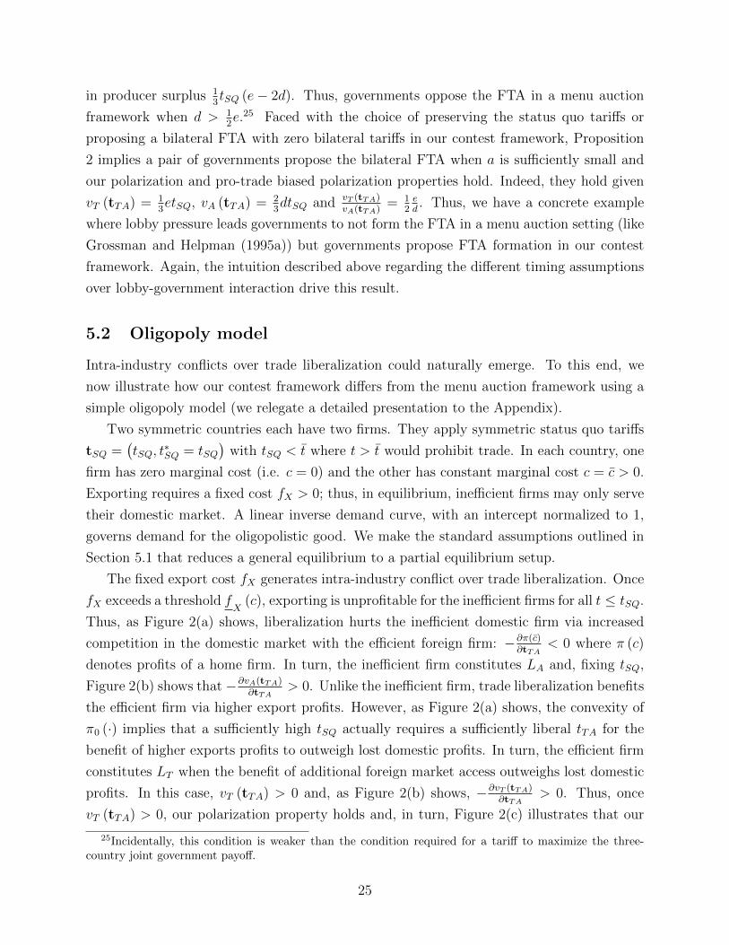
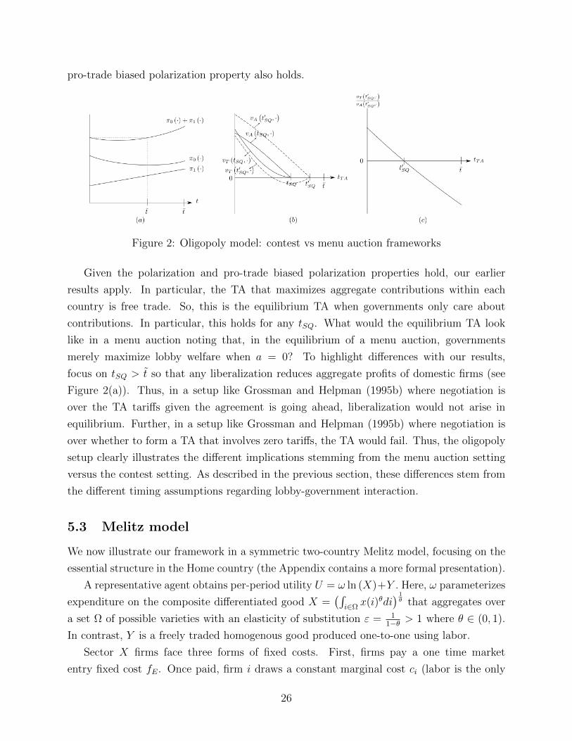
Intra-industry conflicts over trade liberalization could naturally emerge. To this end, we

now illustrate how our contest framework differs from the menu auction framework using a

simple oligopoly model (we relegate a detailed presentation to the Appendix).

Two symmetric countries each have two firms. They apply symmetric status quo tariffs

tSQ =(tSQ, t

∗SQ = tSQ

)with tSQ < t where t > t would prohibit trade. In each country, one

firm has zero marginal cost (i.e. c = 0) and the other has constant marginal cost c = c > 0.

Exporting requires a fixed cost fX > 0; thus, in equilibrium, inefficient firms may only serve

their domestic market. A linear inverse demand curve, with an intercept normalized to 1,

governs demand for the oligopolistic good. We make the standard assumptions outlined in

Section 5.1 that reduces a general equilibrium to a partial equilibrium setup.

The fixed export cost fX generates intra-industry conflict over trade liberalization. Once

fX exceeds a threshold fX

(c), exporting is unprofitable for the inefficient firms for all t ≤ tSQ.

Thus, as Figure 2(a) shows, liberalization hurts the inefficient domestic firm via increased

competition in the domestic market with the efficient foreign firm: −∂π(c)∂tTA

< 0 where π (c)

denotes profits of a home firm. In turn, the inefficient firm constitutes LA and, fixing tSQ,

Figure 2(b) shows that −∂vA(tTA)∂tTA

> 0. Unlike the inefficient firm, trade liberalization benefits

the efficient firm via higher export profits. However, as Figure 2(a) shows, the convexity of

π0 (·) implies that a sufficiently high tSQ actually requires a sufficiently liberal tTA for the

benefit of higher exports profits to outweigh lost domestic profits. In turn, the efficient firm

constitutes LT when the benefit of additional foreign market access outweighs lost domestic

profits. In this case, vT (tTA) > 0 and, as Figure 2(b) shows, −∂vT (tTA)∂tTA

> 0. Thus, once

vT (tTA) > 0, our polarization property holds and, in turn, Figure 2(c) illustrates that our

25Incidentally, this condition is weaker than the condition required for a tariff to maximize the three-country joint government payoff.

25

pro-trade biased polarization property also holds.

Figure 2: Oligopoly model: contest vs menu auction frameworks

Given the polarization and pro-trade biased polarization properties hold, our earlier

results apply. In particular, the TA that maximizes aggregate contributions within each

country is free trade. So, this is the equilibrium TA when governments only care about

contributions. In particular, this holds for any tSQ. What would the equilibrium TA look

like in a menu auction noting that, in the equilibrium of a menu auction, governments

merely maximize lobby welfare when a = 0? To highlight differences with our results,

focus on tSQ > t so that any liberalization reduces aggregate profits of domestic firms (see

Figure 2(a)). Thus, in a setup like Grossman and Helpman (1995b) where negotiation is

over the TA tariffs given the agreement is going ahead, liberalization would not arise in

equilibrium. Further, in a setup like Grossman and Helpman (1995b) where negotiation is

over whether to form a TA that involves zero tariffs, the TA would fail. Thus, the oligopoly

setup clearly illustrates the different implications stemming from the menu auction setting

versus the contest setting. As described in the previous section, these differences stem from

the different timing assumptions regarding lobby-government interaction.

5.3 Melitz model

We now illustrate our framework in a symmetric two-country Melitz model, focusing on the

essential structure in the Home country (the Appendix contains a more formal presentation).

A representative agent obtains per-period utility U = ω ln (X)+Y . Here, ω parameterizes

expenditure on the composite differentiated good X =(∫

i∈Ωx(i)θdi

) 1θ that aggregates over

a set Ω of possible varieties with an elasticity of substitution ε = 11−θ > 1 where θ ∈ (0, 1).

In contrast, Y is a freely traded homogenous good produced one-to-one using labor.

Sector X firms face three forms of fixed costs. First, firms pay a one time market

entry fixed cost fE. Once paid, firm i draws a constant marginal cost ci (labor is the only

26

input) from the Pareto distribution G(c) =(

ccU

)kwith 0 < c < cU and shape parameter k

> (ε−1). Thus, a competitive fringe of potential entrants awaits favorable market conditions

to make entry profitable. Second, after observing ci, firm i decides whether to produce

knowing production incurs a per-period fixed cost fD. Thus, in response to adverse changes

in market conditions, relatively unproductive firms exit the market. Third, firm i pays an

additional fixed cost fX = γfD if it serves the foreign market. Because γ > 1, any firm

that produces will serve the domestic market and only the most productive firms export.

Summarizing, the three key parameters in the model are (i) the elasticity of substitution

between differentiated varieties ε = 11−θ > 1, (ii) γ = fX

fD, capturing the additional cost of

exporting relative to domestic production and (iii) the Pareto shape parameter k, governing

the dispersion of firm productivity.

5.3.1 Equilibrium and lobbying

Zero profit conditions and a free entry condition allow closing the model and the Pareto

distribution for marginal cost allows closed form solutions. Conditional on a set of firms

having paid the fixed market entry cost fE, zero profit conditions pin down the marginal

cost cutoffs that define firm production choices. Given the status quo tariffs tSQ, (i) firms

with ci ≤ cX,SQ serve the domestic market and export, (ii) firms with ci ∈ (cX,SQ, cD,SQ]

only serve the domestic market, and (iii) firms with ci > cD,SQ exit without producing.

Importantly, these zero profit conditions are zero ‘operating’ profit which do not take into

account the fixed market entry cost fE. The free entry condition determines the mass of

firms NE,SQ that enter and force a potential entrant’s expected operating profit to equal the

fixed market entry cost fE. The Appendix presents derivations and closed form solutions for

cX,SQ, cD,SQ and NE,SQ and the associated profits for the different types of firms.

Upon implementation of the TA tariffs tTA, we can solve for new marginal cost cutoffs

cX,TA and cD,TA. In doing so, one must take a stand on how the mass of firms, NE, adjusts.

First, one could take a ‘short-run’ view that holds NE,SQ fixed.26 Second, one could take

a ‘long-run’ view that allows NE to adjust given the new market conditions. In this latter

case, we assume that only the mass of firms NE,SQ lobby over the TA. To do otherwise would

allow the seemingly unrealistic possibility that ‘potential’ firms, i.e. those who are not yet

producing anything, lobby over the TA. Having solved for the endogenous marginal cost

cutoffs, as well as other endogenous variables, we again obtain closed form solutions for the

profits of the different types of firms.

To define lobby group valuations, let c denote the threshold marginal cost for a firm

26Holding NE fixed in the ‘short-run’ is similar to Eaton and Kortum (2005), Chaney (2008), Do andLevchenko (2009) and Arkolakis et al. (2012).

27

indifferent between the TA tariffs tTA and the status quo tariffs tSQ. Further, let π (c, (t, t∗))

denote a firm’s operating profit with marginal cost c and tariffs (t, t∗). Then, LA (LT )

constitutes firms with marginal cost above (below) c and their valuations are

vA = NE

∫ cD,SQ

c

(π (c, tSQ)− π (c, tTA)) dG (c) (21)

vT = NE

∫ c

0

(π (c, tTA)− π (c, tSQ)) dG (c) . (22)

To ensure that vT (tTA) > vA (tTA), we impose tSQ <kk−θ .

Given this assumption, we numerically investigate the properties imposed in our earlier

analysis: (i) a more liberal TA polarizes the lobby groups, −∂vi (tTA) /∂tTA > 0 for i ∈A, T, and (ii) a more liberal TA generates pro-trade biased polarization: −∂ vT (tTA)

vA(tTA)/∂tTA ≥

0.27 In the ‘long-run’, these properties hold without any restrictions.28 In the short-run case,

the former property fails for the anti-trade lobby as the equilibrium mass of non-exporting

firms vanish. Intuitively, we need a non-trivial mass of ‘import-competing’ firms for a more

liberal TA to strengthen the anti-trade lobby’s TA opposition.29 Thus, this condition appears

rather unrestrictive. In turn, application of Proposition 2 implies that the equilibrium TA

is free trade in the symmetric Melitz model as long as a is sufficiently small, γ is sufficiently

large, and TA tariffs respect the reciprocity rule u (tTA; tSQ).

5.3.2 Comparative statics

While free trade is the equilibrium TA, the probability of TA ratification depends on the

relative valuations vT (tTA)vA(tTA)

in Home andv∗T (tTA)

v∗A(tTA)in Foreign. Thus, we can investigate how the

model’s parameters affect the probability of TA formation.

For the ‘short-run’ cases, we can numerically show that (i) d vT (tTA)vA(tTA)

/dγ < 0, so that larger

barriers to exporting decrease the probability of TA formation, (ii) d vT (tTA)vA(tTA)

/dk < 0, so that

more dispersion in firm productivity decreases the probability of TA formation, and (iii)

d vT (tTA)vA(tTA)

/dε > 0, so that a higher willingness to substitute between varieties increases the

probability of TA formation.30 Intuitively, we can think of these results working through the

marginal cost cutoff for an exporter relative to a non-exporter and, in turn, the composition

27Note, the reciprocity rule of equal changes in imports requires symmetric tariff reductions.28Indeed, free entry implies aggregate profits are fixed and thus vT (·) = vA(·) and −∂ vT (tTA)

vA(tTA)/∂tTA = 0.29In general, the anti-trade lobby in the Melitz model consists of low productivity exporting firms and non-

exporting firms. The latter set of firms constitutes what one would normally think of as ‘import-competing’firms.

30For the ‘long-run’ cases, vT (tTA)vA(tTA) = 1 and is independent of the parameters.

28

of firms across the anti-trade and pro-trade lobbies.31 Larger barriers for becoming an

exporter (i.e. higher γ) make it tougher to be an exporter, thereby shifting firm composition

towards non-exporters and lowering vT (tTA)vA(tTA)

. A higher k skews firm composition towards

low productivity firms, making it tougher to be an exporter and lowering vT (tTA)vA(tTA)

. With

consumers more willing to substitute between varieties (i.e. higher ε), markups fall which

disproportionately hurts low productivity firms and induces exit. In turn, firm composition

shifts towards high productivity export firms and raises vT (tTA)vA(tTA)

. These comparative statics

illustrate how one could start thinking about taking our framework to the data.

6 Conclusion

Once governments sign a TA, the ratification process in each country is often lengthy and un-

certain. Illustrative examples include the TPP, US FTAs with Korea and Central America

and the 1994 Uruguay Round. Motivated by these stylized facts, we develop a new two-

country political economy framework with two key features. First, pro-trade and anti-trade

interest groups make contributions to influence their own government’s subsequent ratifica-

tion decision. Second, these interest groups recognize that the TA’s ultimate fate depends

on the ratification decisions of both governments. The former feature distinguishes our con-

test framework from the standard approach in the trade and political economy literature

where the ratification process is ignored and interest groups condition their contributions on

their government’s policy decision. The latter feature distinguishes our framework from the

prior contest literature by linking the outcome in one contest to the outcome in a different

‘parallel’ contest and gives rise to the new class of contests that we call ‘parallel contests’.

In our framework, anti-trade and pro-trade interest groups make contributions in equi-

librium and uncertainty prevails over the ratification decision of each government. These

features match both the contesting real world lobbying interests during the TA ratification

process and the uncertainty over the outcome of this process. In contrast, the benchmark

political economy model in the literature predicts that either the anti-trade or pro-trade

interest group lobbies in equilibrium and there is no uncertainty over a government’s TA

ratification decision (e.g. Grossman and Helpman (1995a)). Thus, our framework offers a

firm foundation for empirical work on the role of lobbying on TA formation.

Regarding the level of negotiated TA tariffs, the key new insight is the lobbying pro-

cess itself drives governments towards proposing the most liberal TA possible. In turn, our

31This relative cutoff is cXcD

=[γ

1ε−1 t

1θ

]−1and the relative mass of exporter to non-exporter firms is

NXND

=(

cXcD

)k.

29

framework suggests that inherent government protectionist tendencies, perhaps driven by

electoral motivations as in Conconi et al. (2014), drive real world protection levels. While

our view of lobbying echoes the typical non-academic view that corporate lobbying drives

liberal trade policy, our view contrasts starkly with the typical view in the literature that

real world protection levels balance protectionist lobbying forces against inherent government

desires for national welfare improving liberalization. Nevertheless, in doing so, our alterna-

tive perspective suggests that the relatively low tariff levels observed across many countries

reflects governments that place relatively large value on lobbying contributions. This offers a

reconciling perspective on the empirical ‘puzzle’ whereby matching data with the benchmark

Protection for Sale framework requires governments have, arguably, implausibly high degrees

of welfare-mindedness.

In a two-country world, Grossman and Helpman (1995b) illustrate the more general point

emphasized by Bagwell and Staiger (1999) that a TA eliminates the terms of trade component

from status quo tariffs but leaves the politics component intact. Nevertheless, we show that,

by leveraging externalities traveling through world prices, our lobbying process can eliminate

the politics component of status quo tariffs. In other words, the TA can itself remove politics

from status quo tariffs by changing the nature of government-lobby interaction from that

underlying the status quo tariffs to that underlying our contest. This difference with the

menu auction setup stems directly from the different timing assumption on government-

lobby interaction: governments receive contributions after their policy decision in a menu

auction but before receiving contributions in a contest framework. In turn, this dichotomy

determines whether a more liberal TA depresses or boosts anti-trade lobby contributions.

Our framework also opens the door to future research directions. Our framework predicts

that the probability of TA formation increases in the strength of pro-trade interest group

support relative to the strength of anti-trade interest group opposition. Given the empiri-

cal economic determinants of FTA literature spawned by Baier and Bergstrand (2004), this

property can drive empirical investigation through the lens of a microfounded political econ-

omy model of FTA formation. Another useful property of our framework is that, as we show

in the all-pay contest setup of the Appendix, one can make predictions about the exten-

sive margin of lobbying; namely, the extent to which interest groups refrain from making

contributions. Again, this prediction lends itself naturally to empirical investigation.

Adding more countries to our framework represents another direction for future research.

In our TA context, a TA with more countries would polarize the anti-trade and pro-trade

lobbies further by increasing the export market access gained and increasing the degree of

import competition. All else equal, this would increase lobbying contributions. However,

on the other hand, by decreasing the likelihood of each country’s TA ratification decision

30

being pivotal, adding more countries would reduce lobbying contributions. Our framework

can analyze the balance between these tensions. These tensions could also be present in

an international environmental agreement like the Kyoto Protocol. Unlike our TA context,

implementation of the Kyoto Protocol only required a two-thirds majority rather than una-

nimity, thereby creating large free riding incentives. Despite being implemented, the US,

the largest CO2 emitter, did not ratify the Kyoto Protocol. Our framework is well suited to

analyze these free riding issues in international negotiations.

Indeed, our parallel contest framework has broad applicability. International agreements

over the environment and safety (e.g. the The Limited Nuclear Test Ban Treaty) share

the basic features of our setup: local interest groups contest each other to influence their

government’s ratification decision knowing implementation of the agreement requires mutual

ratification. A between-firm example is the collaboration between British Aerospace, MBB

of West Germany, and Aeritalia of Italy to produce the Panavia Tornado fighter jet. One

could imagine within-firm divergent views over the balance between collaboration among

Europe’s best military aircraft producers and concerns over proprietary knowledge and/or

national security. A within-firm example is the collaboration of architectural and engineering

departments of the London-based firm Arup who built The Shard. One could imagine tension

within each department arising from some agents wanting to abandon The Shard in favor

of other projects, yet moving ahead with The Shard requires agreement of both department

heads. Interest groups contesting to influence their own decision maker and collaboration

requiring approval of both decision makers ties these examples into a ‘parallel contest’.

Our framework also invites reflection on the extent of possible coordination between

groups in different entities whose interests are aligned (e.g. pro-collaboration groups across

firms or across departments within a firm). Our parallel contest insights inform the nature of

strategic interaction between such groups who cannot perfectly coordinate whereas the well-

known Colonel Blotto game does so in an environment of perfect coordination. However,

an ideal framework would allow flexibility in the degree of imperfect coordination. For

example, in a between-firm collaboration setting, interest groups of one firm may not be

able to lobby the other firm’s decision maker but could perhaps undertake actions that make

it easier for their aligned interest group in the other firm to lobby their own decision maker.

An interesting question becomes whether, as the scope for ‘cross-subsidization’ rises, the

predictions move from those of a parallel contest towards those of the Colonel Blotto game.

31

Appendix

A Proofs from main text

Proof of Proposition 1

Proof. Focusing on the home country without loss of generality,

G (tTA; tSQ) = l(p∗T (tTA), tTA) = p∗T (tTA)1

2v (tTA)

given a = 0 and (6)-(8). Two observations establish the proposition. First, pT (tTA) =[1 + vA(tTA)

vT (tTA)

]−1

follows from (6)-(8) and, by analogy, p∗T (tTA) =[1 +

v∗A(tTA)

v∗T (tTA)

]−1

. Thus, the

pro-trade biased polarization property implies p∗T (tTA) is maximized by the most liberal TA

satisfying u (tTA). Second, the polarization property implies v (tTA) =[

12

(1

vT (tTA)+ 1

vA(tTA)

)]−1

is maximized by the most liberal TA, tTA, satisfying u (tTA). Thus, G (tTA; tSQ) and, by

analogy, G∗ (tTA; tSQ) are maximized by the most liberal TA satisfying u (tTA). In turn, the

restriction tTA ≥ 1 implies tTA = 1 and/or t∗TA = 1.

Proof of Proposition 2

Proof. Focusing on the home country without loss of generality, (16) says −∂G(tTA;tSQ)∂tTA

=

−∂l(p∗T (tTA),tTA;a=0)∂tTA

+ a∂Φ(tTA;tSQ)

∂tTAwhere (17) defines Φ (tTA; tSQ). The proof of Proposition

1 establishes −∂l(p∗T (tTA),tTA;a=0)∂tTA

> 0 for all tTA ≤ tSQ such that tTA satisfies u (tTA). Thus,

G (tTA; tSQ) is maximized by the most liberal TA satisfying u (tTA) for sufficiently small

a > 0 if

∣∣∣∣lima→0∂Φ(tTA;tSQ)

∂tTA

∣∣∣∣ 6=∞. Note that

∂Φ (·)∂tTA

= −∆h (·)[∂p∗T (tTA)

∂tTApT (tTA) +

∂pT (tTA)

∂tTAp∗T (tTA)

](23)

= −∆h (·)

(∂lT (·;a=0)∂tTA

− a∂hT (·)∂tTA

)lA (·)− ∂lA(·;a=0)

∂tTAlT (·)(

lA (·) + lT (·))2

+

(∂l∗T (·;a=0)

∂tTA− a∂h

∗T (·)

∂tTA

)l∗A (·)− ∂l∗A(·;a=0)

∂tTAl∗T (·)(

l∗A (·) + l∗T (·))2

.where li (·; a = 0) , l∗i (·; a = 0) , hi (·) , h∗i (·) ∈ R for i ∈ A, T and independent of a. Further,

32

li (·) , l∗i (·) > 0 for i ∈ A, T and for any a ≥ 0. Combined with ∂li(·;a=0)∂tTA

,∂l∗i (·;a=0)

∂tTA, ∂hT (·)∂tTA

,∂h∗T (·)∂tTA

∈ R we have lima→0∂Φ(·)∂tTA

∈ R. In turn, lima→0 a∂Φ(·)∂tTA

= 0. Hence, for sufficiently small

a > 0, G (tTA; tSQ) is maximized by the most liberal TA satisfying u (tTA), denoted tTA.

The restriction tTA ≥ 1 implies tTA = 1 and/or t∗TA = 1.

Finally, substituting (13)-(14) into (12), and remembering si = li + ahi, establishes

pT (tTA) =[1 + vA(tTA)

vT (tTA)

]−1

and, by analogy, p∗T (tTA) =[1 +

v∗A(tTA)

v∗T (tTA)

]−1

.

B The Extensive Margin of a TA Contest

In our Tullock contest setting, i.e. r = 1, only the intensive margin of lobbying appeared.

However, moving to an all pay contest by letting r → ∞ introduces the extensive margin

of lobbying because interest groups may refrain from making contributions in equilibrium.

Letting r →∞ and using (1):

pT =

0 if sT < sA

1 if sT > sA

ρ ∈ (0, 1] if sT = sA

.

We now investigate various forms of our parallel all pay contest.

The ‘all-pay contest’ literature builds on the ‘all-pay auction’ literature by generalizing

the cost function of a bid/contribution beyond the bid/contribution itself. Hillman and

Samet (1987), Hillman and Riley (1989) and Baye et al. (1996) pioneered the all-pay auction

literature to model rent-seeking and lobbying activities. For example, Hillman (2013) argues

unilateral trade policy can be viewed as an all-pay auction. Siegel (2009, 2010, 2014) develops

the theory of all-pay contests by allowing the cost of contributions to vary across players.

This generalization allows some players to have a ‘head start’ over others.

B.1 All pay auctions: no head starts

In the absence of head starts, si = li, the all pay contest reduces to an all pay auction and

their equilibrium characterization was developed by Hillman and Riley (1989) and Baye et al.

(1996). As described in the main text, the standard solution techniques and theorems used

therein apply in our parallel contest because the preferences underlying the expected payoff

functions are identical to those in a standard all pay auction where the exogenous valuations

are given by our exogenous ‘effective’ valuations vi (tTA).

As is well known in the literature, the standard all pay auction has no pure strategy

equilibrium. Intuitively, given the deterministic nature of the Home government’s TA rati-

33

fication decision, Home lobbies only want to contribute if they are successful in swaying the

Home government’s ratification decision. That is, fixing the positive probability of Foreign

ratification, each Home lobby prefers not contributing rather than making a contribution ar-

bitrarily lower than the other lobby because any such contribution does not sway the Home

government’s ratification decision. However, in turn, the lobby that succeeds in swaying

the government’s decision will make an arbitrarily small contribution. The lack of a pure

strategy equilibrium now becomes clear because the so-called ‘unsuccessful’ lobby benefits

from becoming the ‘successful’ lobby through a contribution slightly above the arbitrarily

small contribution of the other lobby. As a result, the Nash equilibrium of the all pay auc-

tion is a mixed strategy equilibrium where lobbies randomize uniformly over an interval.

Because these randomization strategies depend on the valuation structure, we now build our

discussion around the valuation structure.

B.1.1 Homogenous valuations: vT (tTA) = vA (tTA)

In Stage 2, each lobby randomizes its contributions uniformly over [0, v (tTA)] or, equivalently,

over [0, p∗Tv (tTA)] where v (tTA) = vT (tTA) = vA (tTA). While no lobby benefits from

contributing above their effective valuation v (tTA), lobby competition forces the upper bound

of their contribution to v (tTA). Moreover, two observations imply each lobby’s lower bound

contribution is zero. First, the lobbies must have equal lower bound contributions because

otherwise the lobby with the larger lower bound could benefit by reducing their lower bound.

Second, given equal lower bound contributions, a lobby’s lower bound contribution never

sways the government’s ratification decision and hence the lower bound must be zero. Thus,

ultimately, the interval [0, v (tTA)] characterizes the intensive margin of lobbying. Moreover,

given the symmetric nature of the homogenous valuations all pay auction, the extensive

margin plays no role in equilibrium. Formally, letting αi denote the probability that li = 0,

we have αA = αT = 0 in equilibrium.

In Stage 1, government incentives for setting TA tariffs match those described earlier.

Given the absence of head starts, the Home government’s expected payoff is merely the

expected equilibrium aggregate lobbying contributions E[l (p∗T (·) , tTA)

]= p∗T (·) v (tTA).

But, the symmetric mixed strategy equilibrium implies pT (·) = p∗T (·) = 12

and, in turn,

E[l (p∗T (·) , tTA)

]= 1

2v (tTA). Thus, we only need the assumption that trade liberalization

polarizes lobby groups to ensure that the most liberal TA possible maximizes lobbying con-

tributions received by governments. Intuitively, because homogeneous valuations pins downvT (tTA)vA(tTA)

as constant, we no longer need the pro-trade biased polarization assumption that we

needed in the Tullock contest setting. Thus, we see that our results in Propositions 1-2 of

the main text are robust to the all pay auction homogenous valuation setting.

34

B.1.2 Heterogenous valuations: vT (tTA) 6= vA (tTA)

Without loss of generality, we now assume vT (tTA) > vA (tTA). This heterogeneity assump-

tion is consistent with our polarization and pro-trade biased polarization properties whereby

a more liberal TA increases vT (tTA), vA (tTA) and also vT (tTA)vA(tTA)

.

In Stage 2, both lobbies randomize their contributions uniformly over [0, vA (tTA)] or,

equivalently, over [0, p∗TvA (tTA)]. As the low valuation lobby, LA never contributes above its

effective valuation p∗TvA (tTA). Thus, despite its higher effective valuation, LT never benefits

from bidding above LA’s effective valuation when trying to sway the government’s ratifica-

tion decision. The same logic from the homogeneous valuations case implies each lobby’s

lower bound contribution remains zero. Thus, the interval [0, p∗TvA (tTA)] characterizes the

intensive margin of lobbying.

The symmetric lobbying strategies at the intensive margin combined with the asymmetric

lobby valuations generate an extensive margin of lobbying. Intuitively, as the low valuation

lobby, LA refrains from lobbying and more so as the relative valuation of the pro-trade

lobby rises. Specifically, αA (tTA) = 1 − vA(tTA)vT (tTA)

while αT = 0. Combining this extensive

lobbying margin with the intensive lobbying margin where the government ratifies the TA

with probability 12

conditional on both lobbies contributing, the unconditional probability of

Home ratification is

pT (tTA) = αA (tTA) + [1− αA (tTA)]1

2= 1− 1

2

vA (tTA)

vT (tTA). (24)

In Stage 1, this extensive margin of lobbying has an important impact on government

preferences over TA tariffs. Expected equilibrium aggregate contributions are

E[l (p∗T , tTA)

]=

1

2p∗TvA (tTA)

[1 +

vA (tTA)

vT (tTA)

]. (25)

Like earlier, these contributions are proportional to p∗T . But, unlike earlier, the proportion-

ality with respect to vA (tTA) now reflects the common upper bound on valuations. In any

case, our polarization and pro-trade biased polarization properties ensure the most liberal

TA maximizes both of these components. But, the square bracketed term says, all else

equal, contributions are decreasing in vT (tTA)vA(tTA)

. Thus, here, pro-trade biased polarization says

a more liberal TA hurts the government’s expected payoff by increasing the probability that

LT refrains from contributing. That is, the extensive margin of lobbying introduced by the

heterogeneous valuations all pay auction interferes with the processes that would otherwise

lead to the most liberal possible TA.

Nevertheless, in reasonable situations, the impact of a more liberal TA increasing the

35

probability of foreign TA ratification via pro-trade biased polarization outweighs the impact

of a more liberal TA reducing the probability of LT refraining from contributing. Specifically,

letting ν (tTA) ≡ vA(tTA)vT (tTA)

< 1 and ν∗ (tTA) ≡ v∗A(tTA)

v∗T (tTA)< 1,

−∂l(p∗T (tTA),tTA)∂tTA

> 0 ⇔ 12∂ν∗(tTA)∂tTA

[1 + ν (tTA)]−[1− 1

2ν∗ (tTA)

]∂ν(tTA)∂tTA

> 0

⇔ f (ν (tTA) , ν∗ (tTA)) ≡ 1+ν(tTA)2−ν∗(tTA)

> ∂ν(tTA)/∂tTA∂ν∗(tTA)/∂tTA

.(26)

With symmetric countries, this condition merely reduces to ν∗ (tTA) = ν (tTA) > 12. An anal-

ogous condition for the foreign country’s TA ratification decision is f ∗ (ν (tTA) , ν∗ (tTA)) ≡2−ν(tTA)1+ν∗(tTA)

< ∂ν(tTA)/∂tTA∂ν∗(tTA)/∂tTA

. Thus, ∂ν(tTA)/∂tTA∂ν∗(tTA)/∂tTA

∈ (f (·) , f ∗ (·)) is a sufficient (but not neces-

sary) condition for a more liberal TA to increase lobbying contributions in the home and

foreign countries, and hence for the most liberal TA to be the equilibrium TA. This sufficient

condition can fail among symmetric countries when lobbies within a country are widely asym-

metric (e.g. ν∗ (tTA) = ν (tTA) < 12) or among widely asymmetric countries. Proposition 3

summarizes our discussion.

Proposition 3 Assume r →∞ and a reciprocity rule u (tTA) that ensures a more liberal TA

polarizes the lobby groups and generates pro-trade biased polarization. Further, for hetero-

geneous valuations, assume ∂ν(tTA)/∂tTA∂ν∗(tTA)/∂tTA

∈ (f (·) , f ∗ (·)) where f (·) defined by (26). Then,

in equilibrium, (i) the extensive margin of lobbying is given by αA (tTA) = 1 − vA(tTA)vT (tTA)

and

αT = 0, (ii) aggregate expected lobbying contributions are 12p∗TvA (tTA)

[1 + vA(tTA)

vT (tTA)

], (iii) the

probability of TA formation is pT (tTA) p∗T (tTA) =[1− 1

2vA(tTA)vT (tTA)

]·[1− 1

2

v∗A(tTA)

v∗T (tTA)

]and (iv) the

Home and Foreign governments propose the most liberal TA possible, denoted tTA, implying

at least one country practices free trade: tTA = 1 and/or t∗TA = 1.

Proof. First, consider the homogenous valuations case of vA (tTA) = vT (tTA) ≡ v (tTA) ,

and v∗A (tTA) = v∗T (tTA) ≡ v∗ (tTA):

(i) Follows from Theorem 1 in Baye et al. (1996), noting that homogeneous valuations

imply αA (tTA) = 1− vA(tTA)vT (tTA)

= 0.

(ii) Given homogenous valuations, E[l (p∗T , tTA)

]= 1

2p∗TvA (tTA)

[1 + vA(tTA)

vT (tTA)

]= p∗Tv (tTA).

By Theorem 1 in Baye et al. (1996) and (i) above, li (p∗T , tTA)

U∼ [0, v (tTA)] for i ∈A, T where v (tTA) = p∗Tv (tTA). Thus, E

[li (p

∗T , tTA)

]= 1

2v (tTA) = 1

2p∗Tv (tTA) for

i ∈ A, T. In turn, E[li (p

∗T , tTA)

]= v (tTA) = p∗Tv (tTA).

36

(iii) Given homogenous valuations, pT (tTA) p∗T (tTA) =[1− 1

2vA(tTA)vT (tTA)

]·[1− 1

2

v∗A(tTA)

v∗T (tTA)

]= 1

4.

Further, pT (tTA) = Pr (lT > lA) = 12

and, analogously, p∗T (tTA) = Pr (l∗T > l∗A) = 12

because li (p∗T , tTA)

U∼ [0, v (tTA)] and l∗i (p∗T , tTA)U∼ [0, v∗ (tTA)] for i ∈ A, T.

(iv) Focusing on the home country without loss of generality, G (tTA; tSQ) = E[l (p∗T (tTA) , tTA)

]= p∗T (tTA) v (tTA) given a = 0. Because p∗T (tTA) is independent of tTA, the polariza-

tion property implies G (tTA; tSQ) is maximized by the most liberal TA that satisfies

u (tTA). The restriction tTA ≥ 1 implies tTA = 1 and/or t∗TA = 1.

Second, consider heterogeneous valuations:

(i) Follows from Theorem 3 in Baye et al. (1996).

(ii) By Theorem 3 in Baye et al. (1996), lT (p∗T , tTA)U∼ [0, vA (tTA)] = [0, p∗TvA (tTA)] while

lA (p∗T , tTA)U∼ [0, vA (tTA)] = [0, p∗TvA (tTA)] with probability αA (tTA) and lA (p∗T , tTA) =

0 with probability 1− αA (tTA). In turn, E[l (p∗T , tTA)

]= 1

2p∗TvA (tTA)+(1− αA (tTA))

12p∗TvA(tTA) = 1

2p∗TvA (tTA)

[1 + vA(tTA)

vT (tTA)

].

(iii) Note the common support when LA and LT lobby and that ratification requires lT > 0.

Thus, pT (tTA) = αA (tTA) (1− αT ) + 12

(1− αA (tTA)) (1− αT ). In turn, pT (tTA) =(1− vA(tTA)

vT (tTA)

)+ 1

2vA(tTA)vT (tTA)

= 1− 12vA(tTA)vT (tTA)

. And, analogously, p∗T (tTA) = 1− 12

v∗A(tTA)

v∗T (tTA).

(iv) Given (25) combined with the polarization property and (26), we have −∂G(tTA;tSQ)∂tTA

> 0

and −∂G∗(tTA;tSQ)∂tTA

> 0 for all tTA ≤ tSQ. Thus, the most liberal TA satisfying u (tTA)

maximizes G (tTA; tSQ) and G∗ (tTA; tSQ). The restriction tTA ≥ 1 implies tTA = 1

and/or t∗TA = 1.

B.2 All pay contests: head starts

When lobby groups have head starts, the government’s ratification decision in Stage 3 de-

pends on the augmented contributions si = li + ahi (·). Effectively, head starts subsidize

the cost of augmented contributions si (the cost is merely li) and distinguish the all pay

contest from an all pay contest. Drawing on novel techniques developed by Siegel (2009,

2010, 2014), we now analyze the all pay contest. For the sake of exposition, we continue to

assume heterogenous valuations where vT (tTA) > vA (tTA) so that LA is the low valuation

37

lobby and that any anti-trade head start does not outweigh the heterogeneity in valuations:

p∗TvT (tTA) + a∆h (tTA; tSQ) > p∗TvA (tTA).32

First, consider the impact of anti-trade head starts a∆h (tTA; tSQ) < 0 in Stage 2. At

the intensive margin, LA still randomizes over [0, p∗TvA] as the low valuation lobby with

a net head start that does not outweigh the valuation difference. However, facing a net

head start disadvantage, LT must contribute −a∆h (tTA; tSQ) and p∗TvA− a∆h (tTA; tSQ) to

compete against, respectively, LA’s lowest and highest contribution. Thus, LT randomizes

over [−a∆h (tTA; tSQ) , p∗TvA − a∆h (tTA; tSQ)]. For the extensive margin, notice the impact

of the anti-trade head start on the highest payoffs that lobbies can guarantee themselves.

For LA, as in the absence of head starts, this zero payoff comes by not contributing. For

LT , as in the absence of head starts with p∗TvT (tTA) > p∗TvA (tTA), this payoff still comes via

a contribution that guarantees Home ratification. But, given the ant-trade head start, this

contribution rises, and the associated payoff falls, by −a∆h (tTA; tSQ) > 0. Importantly,

the adjustment at the intensive margin perfectly reflects these effects: the probability of

Home ratification remains 12

with LA’s expected contributions remaining unchanged but

LT ’s expected contributions rising by −a∆h (tTA; tSQ) > 0. Thus anti-trade head starts

impact the intensive margin but not the extensive margin so that, in turn, TA ratification

probabilities (in Stage 3) and the equilibrium TA (in Stage 1) mirror our earlier analysis.

Second, consider the impact of pro-trade head starts a∆h (tTA; tSQ) > 0 in Stage 2. At

the intensive margin, as the low valuation lobby facing a net head start disadvantage, LA

adjusts its lower bound upward to compete with LT ’s zero contribution and, thus, randomizes

over [a∆h (tTA; tSQ) , p∗TvA]. Further, because of its head start advantage, LT adjusts its

upper bound downwards to compete against LA’s highest contribution and, thus, randomizes

over [0, p∗TvA − a∆h (tTA; tSQ)]. For the impact at the extensive margin, notice that the

increase in LA’s expected contribution implies that, absent any adjustment at the extensive

margin, it would benefit from not contributing and ensuring a zero payoff. The required

adjustments at the extensive margin imply αA (tTA; tSQ) = 1 − vA(tTA)vT (tTA)

[1− a∆h(tTA;tSQ)

p∗T vA(tTA)

]and αT (tTA; tSQ) =

a∆h(tTA;tSQ)p∗T vA(tTA)

so that these adjustments rise with the size of the pro-

trade head start a∆h (tTA; tSQ). Proposition 4 summarizes this discussion.

Proposition 4 Assume r → ∞ and a reciprocity rule u (tTA) that ensures a more liberal

TA polarizes the lobby groups and generates pro-trade biased polarization. Further, assume∂ν(tTA)/∂tTA∂ν∗(tTA)/∂tTA

∈ (f (·) , f ∗ (·)) where f (·) defined by (26). Then, in equilibrium,

(i) the extensive margin of lobbying is given by αA (tTA) = 1 − vA(tTA)vT (tTA)

and αT (tTA) = 0

32This latter assumption implies LA is the ‘marginal’ lobby in Siegel’s terminology.

38

when a∆h (tTA; tSQ) < 0 but αA (p∗T , tTA; tSQ) = 1 − vA(tTA)vT (tTA)

[1− a∆h(tTA;tSQ)

p∗T vA(tTA)

]and

αT (p∗T , tTA; tSQ) =a∆h(tTA;tSQ)p∗T vA(tTA)

when a∆h (tTA; tSQ) > 0;

(ii) expected aggregate contributions differ from those when a = 0 by a∆h (tTA; tSQ);

(iii) the probability of Home TA ratification (and analogously for Foreign) is pT (tTA) = 1−12vA(tTA)vT (tTA)

when a∆h (tTA; tSQ) < 0 but pT (p∗T , tTA; tSQ) = 1−12vA(tTA)vT (tTA)

[1−

(a∆h(tTA;tSQ)p∗T vA(tTA)

)2]

when a∆h (tTA; tSQ) > 0;

(iv) for sufficiently small a > 0, the Home and Foreign governments propose the most

liberal TA possible, denoted tTA, implying that at least one country practices free trade:

tTA = 1 and/or t∗TA = 1.

Proof. First, consider the anti-trade head start case, a∆h (tTA; tSQ) < 0.

(i) Follows from the algorithm in Siegel (2014).

(ii) Following the algorithm in Siegel (2014), lT (p∗T , tTA; tSQ)U∼ [−a∆h (tTA; tSQ) , vA (tTA)−

a∆h (tTA; tSQ)] where vA (tTA) = p∗TvA (tTA) while lA (p∗T , tTA; tSQ)U∼ [0, vA (tTA)] with

probability αA (tTA) and lA (p∗T , tTA; tSQ) = 0 with probability 1− αA (p∗T ). Thus,

E[l (p∗T , tTA; tSQ)

]=

1

2[p∗TvA (tTA)− 2a∆h (tTA; tSQ)] + (1− αA (tTA))

1

2p∗TvA

=1

2p∗TvA (tTA)

[1 +

vA (tTA)

vT (tTA)

]− a∆h (tTA; tSQ) .

(iii) When lobbying with positive probability, (i) above establishes that lA (p∗T , tTA; tSQ)

and lT (p∗T , tTA; tSQ) have common support and, hence, so do sA (p∗T , tTA; tSQ) and

sT (p∗T , tTA; tSQ). Thus, pT (tTA) = αA (tTA) [1− αT (tTA)]+12

[1− αA (tTA)] [1−αT (tTA)]

given ∆h (tTA; tSQ) < 0 and that ratification requires lT > 0. In turn,

pT (tTA) =

(1− vA (tTA)

vT (tTA)

)+

1

2

vA (tTA)

vT (tTA)= 1− 1

2

vA (tTA)

vT (tTA).

(iv) Given (ii) above, equations (16)-(18) apply as in the main text. Focusing on the Home

country’s perspective without loss of generality and combining∂p∗T (tTA)

∂tTA,∂∆h(tTA;tSQ)

∂tTA∈

R and independent of a with the logic from the proof of Proposition 2(iii), we have

lima→0∂Φ(·)∂tTA

∈ R. In turn, lima→0 a∂Φ(·)∂tTA

= 0. Further, note that −∂l(p∗T (tTA),tTA;a=0)∂tTA

> 0

39

for all tTA ≤ tSQ such that tTA satisfies u (tTA). Thus, for sufficiently small a > 0,

G (tTA; tSQ) and G∗ (tTA; tSQ) are maximized by the most liberal TA satisfying u (tTA),

denoted tTA, when ∂ν(tTA)/∂tTA∂ν∗(tTA)/∂tTA

∈ (f (·) , f ∗ (·)). The restriction tTA ≥ 1 implies

tTA = 1 and/or t∗TA = 1.

Second, consider the pro-trade head start case, a∆h (tTA; tSQ) > 0.

(i) Follows from the algorithm in Siegel (2014).

(ii) Following the algorithm in Siegel (2014), lT (p∗T , tTA; tSQ)U∼ [0, vA (tTA)− a∆h (tTA; tSQ)]

where vA (tTA) = p∗TvA (tTA) with probability 1−αT (p∗T , tTA; tSQ) and lT (p∗T , tTA; tSQ) =

0 with probability αT (p∗T , tTA; tSQ) while lA (p∗T , tTA; tSQ)U∼ [a∆h (tTA; tSQ) , vA (tTA)]

with probability αT (p∗T , tTA; tSQ) and lA (p∗T , tTA; tSQ) = 0 with probability 1− αT (·).Thus,

E[l (·)]

=1

2[p∗TvA (tTA)− 2a∆h (tTA; tSQ)] + [1− αA (p∗T , tTA; tSQ)]

1

2p∗TvA (tTA)

=1

2p∗TvA (tTA)

[1 +

vA (tTA)

vT (tTA)

]− a∆h (tTA; tSQ) .

(iii) Given lT (p∗T , tTA; tSQ) and lA (p∗T , tTA; tSQ) when lobbying with positive probability

from (ii) above,

sT (p∗T , tTA; tSQ)U∼ [ahT (tTA) , p∗TvA (tTA) + ahA (tSQ)] , and

sA (p∗T , tTA; tSQ)U∼ [ahT (tTA) , p∗TvA + ahA (tSQ)]

have common support. Thus, pT (p∗T , tTA; tSQ) = αA (p∗T , tTA; tSQ) [1−αT (p∗T , tTA; tSQ)]+12

[1− αA (p∗T , tTA; tSQ)] [1− αT (p∗T , tTA; tSQ)] given ∆h (tTA; tSQ) > 0 and that ratifi-

cation requires lT > 0. In turn,

pT (p∗T , tTA; tSQ) = 1− 1

2

vA (tTA)

vT (tTA)

[1−

(a∆h (tTA; tSQ)

p∗TvA (tTA)

)2]

p∗T (pT , tTA; tSQ) = 1− 1

2

v∗A (tTA)

v∗T (tTA)

[1−

(a∆h∗ (tTA; tSQ)

pTv∗A (tTA)

)2].

(iv) Given (ii) above, equations (16)-(18) apply as in the main text. Here, we focus on the

Home country’s perspective without loss of generality. Given p∗T (pT , tTA; tSQ), then

40

pT (p∗T , tTA; tSQ) is an implicit function. Thus, letting

f (·) = pT (p∗T , tTA; tSQ)− 1 +1

2

vA (tTA)

vT (tTA)

[1−

(a∆h (tTA; tSQ)

p∗T (pT , tTA; tSQ) vA (tTA)

)2],

we have

∂f (·)∂pT

= 1− vA (tTA)

vT (tTA)

v∗A (tTA)

v∗T (tTA)

(a∆h (tTA; tSQ)

vA (tTA)

)2(a∆h∗ (tTA; tSQ)

v∗A (tTA)

)21

p∗T (·)4 pT (·)3

and, given lima→0 pT (p∗T , tTA; tSQ) = lima→0 p∗T (pT , tTA; tSQ) > 0, we have lima→0

∂f(·)∂pT

=

1. Further,

∂f (·)∂tTA

=1

2

∂ [vA (tTA) /vT (tTA)]

∂tTA

[1−

(a∆h (tTA; tSQ)

p∗T (·) vA (tTA)

)2]

− 1

2

vA (tTA)

vT (tTA)

(a

p∗T (·)

)2∂ [∆h (tTA; tSQ) /vT (tTA)]

∂tTA

where lima→0∂f(·)∂tTA

= 12∂[vA(tTA)/vT (tTA)]

∂tTA. Thus, by the implicit function theorem, ∂pT

∂tTA=

−∂f(·)/∂tTA∂f(·)/∂pT

where lima→0∂pT∂tTA

= 12∂(vA/vT )∂tTA

. In turn, using (23), lima→0∂Φ∂tTA

> 0 and

lima→0 a∂Φ∂tTA

= 0. Further, note that−∂l(p∗T (tTA),tTA;a=0)∂tTA

> 0 for all tTA ≤ tSQ such that

tTA satisfies u (tTA). Hence, for sufficiently small a > 0, G (tTA; tSQ) and, by analogous

logic, G∗ (tTA; tSQ) are maximized by the most liberal TA satisfying u (tTA), denoted

tTA, when ∂ν(tTA)/∂tTA∂ν∗(tTA)/∂tTA

∈ (f (·) , f ∗ (·)). The restriction tTA ≥ 1 implies tTA = 1 and/or

t∗TA = 1.

C Examples of particular underlying trade models

In this section, we illustrate how the generality of our contest framework allows for a variety

of popular trade models, including general equilibrium and partial equilibrium specific factors

models, the oligopoly model and the Melitz model.

41

C.1 Specific Factors Models

C.1.1 General equilibrium model

Consider two sectors, X and Y , produced using labor and a specific factor KX and KY re-

spectively. Formally, X = F(LX , KX

)and Y = G

(LY , KY

)subject to the full employment

condition L = LX + LY where (i) FL > 0 and GL > 0, (ii) FLL < 0 and GLL < 0 and (iii)

FKL > 0 and GKL > 0 with the subscripts K and L denoting partial derivatives.

Profit maximization by firms gives the following equilibrium factor price conditions:

wX = pXFL, rX = pXFK , wY = pYGL and rY = pYGK where the subscripts X and Y

denote the sector. Labor mobility also implies wage equalization, so wX = wY and, in turn,

h (pX , pY , LX) ≡ pXFL(LX , KX

)− pYGL

(L− LX , KY

)= 0. Thus,

∂LX∂pX

= − ∂h/∂pX∂h/∂LX

= − FLpXFLL + pYGLL

> 0 and∂LX∂pY

= − ∂h/∂pY∂h/∂LX

=GL

pXFLL + pYGLL

< 0.

What are the impacts of tariffs on real factor incomes for the specific factors? Without

loss of generality, suppose the home country imports good X. Then, assuming the home

country is small, the local price is pX = p∗X + t where p∗X is the world price of good X and t

is the tariff. Then, for any variable z, we have dzdt

= dzdpX

dpXdt

= dzdpX

. In turn, we have:

d rXpX

dpX= FKL

∂LX∂pX

> 0 andd rXpY

dpX=dFKdpX

pXpY

+ FK1

pY> 0 (27)

d rYpY

dpX= GKL

∂LY∂pX

< 0 andd rYpX

dpX=dGK

dpX

pYpX−GK

pYpX

1

pX< 0. (28)

Note, these results hold for any marginal tariff reduction. Hence, consider a tariff reduction

from t0 to t1. And, without loss of generality given (27)-(28), let the exportable good Y be the

numeraire and choose its units of measurement so that p∗Y = 1. Then, the real income changes

associated with a TA are vT = KY ·(rY (t1)− rY (t0)) > 0 and vA = KX ·(rX (t0)− rX (t1)) >

0. Finally, fixing t0, vT and vA are decreasing in t1 which establishes our polarization property.

Note that, in the limit as t1 − t0 gets arbitrarily small, we have (letting good Y be

the numeraire) vT = −KY∂GK∂pX

> 0 and vA = KX∂(pXFK)∂pX

> 0. For our pro-trade biased

42

polarization property, we want to show∂vTvA

∂pX< 0:

∂ vTvA

∂pX∝ ∂vT

∂pXvA −

∂vA∂pX

vT < 0

⇒ −KY∂2GK

∂p2X

· KX∂ (pXFK)

∂pX+ KX

∂2 (pXFK)

∂p2X

· −KY∂GK

∂pX< 0

⇒ −∂GK

∂pX

[∂2GK

∂p2X

]−1

> −∂ (pXFK)

∂pX

[∂2 (pXFK)

∂p2X

]−1

. (29)

Note that, given vT and vA are both positive and decreasing in pX , both sides of (29) are

positive. Thus, pro-trade biased polarization requires that, as the tariff decreases and labor

shifts into the comparative advantage sector Y then VMPKY = pYGK increases at a faster

rate than the rate at which VMPKX = pXFK falls. Put simply, the free trade production

point cannot get too close to the corner of the PPF.

C.1.2 Two country partial equilibrium model

Each country i has a ‘comparative advantage’ good Z = I with an endowment eZi = e > 0

and a ‘comparative disadvantage’ in any good Z 6= I with an endowment eZi = d > 0.

Demand curves in each country i are qIi = α − pIi and, for Z 6= I, qZi = θ − pZi . No

arbitrage conditions link equilibrium cross-country local prices of each good and balanced

trade determines equilibrium local prices. In turn, country i’s national welfare Wi (·) is then

given by the sum of consumer surplus CSi (·), producer surplus of the export and import-

competing sectors PSXi (·) and PSMi (·), and tariff revenue TRi (·). With two countries z =

i, j and two goods Z = I, J we have

CSi (·) =1

8[(θ − α) + (e+ d)− tij]2 +

1

8[(α− θ) + (e+ d)− tji]2 ,

PSXi (·) =1

2e [(α + θ)− (e+ d)− tji] ,

PSMi (·) =1

2d [(α + θ)− (e+ d) + tij]

TRi (·) = tij [(θ − α) + (e− d)− tij]

and analogously for country j. In turn, vT = PSXi (tTA, ·) − PSXi (tSQ, ·) = 12e (tSQ − tTA)

and vA = PSMi (tSQ, ·)− PSMi (tTA, ·) = 12d (tSQ − tTA).

In a symmetric Protection for Sale setting, tSQ maximizes Gi (tSQ, ·) = PSIi (tSQ, ·) +

PSJi (tSQ, ·) + aWi (tSQ, ·) while tTA maximizes Gi (tTA, ·) + Gj (tTA, ·). This yields tGHSQ =13

[(θ − α) + (e− d)− d

a

]+ d

aand tGHTA = d−e

a. Because of our linear structure, the terms of

43

trade effect, i.e. the inverse export supply elasticity faced by the importer, is merely equal

to the level of imports: tGHTOT = 13

[(θ − α) + (e− d)− d

a

]. Thus, tGHTA eliminates tGHTOT from

tGHSQ and merely combines the politics effects of home da

and foreign − ea.

In our setting, tSQ is exogenous while tTA maximizes Gi (tTA, ·) + Gj (tTA, ·) where, for

the Home country, Gi (tTA, ·) = lT (p∗T (tTA) , tTA, ·) + lA (p∗T (tTA) , tTA, ·) +aWi (tTA, ·). Note

that our polarization and pro-trade biased polarization properties hold: −∂vT (tTA)∂tTA

> 0,

−∂vA(tTA)∂tTA

> 0 and −∂[vT (tTA)/vA(tTA)]∂tTA

= 0. Thus, Proposition 2 implies tTA = 0.

C.1.3 Three country partial equilibrium model

The setup is the same as the two country case except we now have three countries z = i, j, k

and three goods Z = I, J,K. In turn,

CSi (·) =1

18[2 (α− θ) + (e+ 2d) + (tji + tki)]

2 +1

18

∑h=j,k;h′ 6=i,h

[(θ − α) + (e+ 2d)− (2tih − th′h)]2 ,

PSXi (·) =1

3e [(2θ + α)− (e+ 2d)− (tji + tki)] ,

PSMi (·) =1

3d∑h=j,k;h′ 6=i,h

[(2θ + α)− (e+ 2d) + (2tih − th′h)] ,

TRi (·) =∑h=j,k;h′ 6=i,h

tih [(θ − α) + (e− d) + (tih − 2tih′)] ,

and analogously for countries j and k. Letting tSQ denote the global tariff vector before the

FTA and tFTA denote the global tariff vector in the presence of an FTA between countries

i and j which now forces tij = tji = 0, we have vT = PSXi (tFTA, ·) − PSXi (tSQ, ·) = 13etSQ

and vA = PSMi (tFTA, ·)− PSMi (tSQ, ·) = 23dtSQ.

With a = 0 in a Protection for Sale setting, Gi (·) = PSXi (·) + PSMi (·) and an FTA

forms if and only if Gi (tFTA, ·) − Gi (tSQ, ·) = 13tSQ (e− 2d) > 0. Thus, an FTA does not

form if d > 12e.

With a = 0 in our setting, the polarization and pro-trade biased polarization properties

hold: − ∂vT∂tTA

> 0, − ∂vA∂tTA

> 0 and −∂vT /vA∂tTA

= 0. Thus, Proposition 2 implies that, in this

three country world, countries i and j would propose a bilateral TA with zero bilateral tariffs.

This is precisely an FTA between countries i and j.

44

C.2 Oligopoly Model

We assume two symmetric countries where country 1 (2) is the home (foreign) country. Two

firms exist in each country: firm 1 has marginal cost c = c > 0 and firm 0 has zero marginal

cost (i.e. c = 0). A firm incurs a fixed cost of exporting fX ≥ 0 so that inefficient firms can

be “domestic only” firms in equilibrium. Each country imposes the common TA tariff tTA

and has a linear inverse demand function with intercept α.

Let xi (c) denote the sales of a home country firm in country i ∈ 1, 2 and x∗i (c) denote

the sales of a foreign country firm in country i. Assume inefficient firms do not export. Then,

local sales by home country firms are (i) x1 (0) > 0 and (ii) x1 (c) > 0 if tTA > 3c− α which

holds if c < 13α . And, export sales of the efficient foreign firm are x∗1 (0) > 0 if tTA <

α+c3

.

Taking these equilibrium quantities as given, the inefficient foreign firm does not export if

π∗1 (c) = (x∗1 (c))2 = 164

[α− 3c− 3tTA]2 < fX . Since π∗1 (c) is maximized at free trade (i.e.

tTA = 0) then a lower bound on fX that ensures π∗1 (c) < fX is fX≡ 1

64[α− 3c]2.

What about our polarization properties? Let π (c) and π∗ (c) denote total profits for,

respectively, a Home and Foreign firm. Then, imposing fX > fX

, inefficient firms are anti-

trade, i.e. vA = π (c; tTA)− π (c; tSQ) > 0, because ∂π(c)∂tTA

> 0 for all tTA if and only if c < 13α

which is the condition required for, regardless of tTA, strictly positive local sales by inefficient

firms. Whether efficient firms are pro-trade depends on tTA: ∂π(0)∂tTA

> 0 iff tTA >α+c

5so that

efficient firms suffer from small tariff cuts when tTA >α+c

5but benefit from marginal tariff

cuts when tTA <α+c

5. Specifically, efficient firms are pro-trade, i.e. vT (0; tTA, tSQ) > 0, if and

only tTA < tSQ − α+c5

. Thus, our polarization properties hold for a well defined area of the

parameter space. And, noting that conditions above required c < 13α, our pro-trade biased

polarization property also holds: −∂vT (·)/vA(·)∂tTA

= 8(3α−7c)

(tSQ+tTA+2α−6c)2 > 0. Hence, Proposition 2

applies.

C.3 Melitz Model

Within-period utility of the representative agent in Home is given by

U = ω ln (X) + Y (30)

where

X =

(∫i∈Ω

x(i, t)θdi

) 1θ

45

aggregates over a set Ω of varieties (potentially) available to the consumer with an elasticity

of substitution ε = 1/(1− θ) where 0 < θ < 1. Demand for each variety in Home is

x(i, t) =

p(i)−εω

P(t)1−εfor domestic firm i

t−ε p(i)−εω

P(t)1−εfor foreign firm i

where p(i) is the producer price charged by a monopolistically competitive firm selling variety

i in Home and P (t)1−ε is the aggregate consumer price index in Home for a symmetric tariff

t imposed by Home and Foreign. An analogous set of equations holds for the foreign country

where, by assumption, ω∗ = ω.

Firms considering entry to sector X face a one time sunk market entry cost fE (measured

in units of labor). If paid, the firm draws a constant marginal cost c from the Pareto

distribution with shape parameter k > ε− 1:

G(c) =

(c

cU

)kfor 0 < c < cU

where ci will denote firm i’s marginal cost draw. Once observed, a firm decides whether

to undertake production. Upon production, it incurs an additional fixed cost fD paid each

period. Additionally, it incurs an additional per-period fixed cost fX = γfD > fD if it serves

the foreign market. Production exhibits constant returns to scale with labor as the only

input.

The decisions of whether to produce and export depend on the associated profits. Given

the wage of 1, the per-period operating profit of firm i in the domestic market is

πD(i, t) =

[(p(i)− ci)ωP (t)1−ε

]p(i)−ε − fD.

In turn, given profit maximization implies a constant markup over marginal cost, p(i) = ciθ

:

πD(i, t) = c1−εi B − fD where B =

1

εθ1−ε

(ω

P (t)1−ε

). (31)

In addition to the fixed cost γfD of exporting, firms also faces a symmetric ad valorem

tariff across countries t > 1. As is common in the literature for tractability, we assume

governments consume the numeraire with tariff revenue. Thus, given profit maximization

implies a constant markup over marginal cost, p(i) = ciθ

, operating profit from exporting for

46

a Home firm is

πX (i, t) = t−εc1−εi B∗ − γfD where B∗ =

1

εθ1−ε

(ω

P∗ (t)1−ε

). (32)

C.3.1 Equilibrium

Status Quo Letting SQ denote the status quo, a firm with marginal cost cD,SQ is indif-

ferent between supplying the domestic market and exiting. Further, a firm with marginal

cost cX,SQ is indifferent between exporting and only supplying the domestic market. Using

equations (31) and (32), cD,SQ and cX,SQ are defined by

fD =ω

ε

[cD,SQ

θPSQ (tSQ)

]1−ε

(33)

γfD =ω

tSQε

[tSQcX,SQθP∗SQ (tSQ)

]1−ε

. (34)

Free entry implies an entrepreneur takes a marginal cost draw if the expected present

value of operating profits exceeds the sunk entry cost fE. We assume firms fully discount

expected period 2 profits so that current period expected profits determine their entry de-

cision.33 The zero-operating profit and free entry conditions close the model. The zero-

operating profit conditions pin down cD,SQ and cX,SQ and the free entry condition pins down

the mass of firms NE taking a marginal cost draw from the Pareto distribution:

NE =

γψtkθSQ + 1

γψtkθSQ + tSQ

( θω

kfE

)(35)

cD,SQ =(γψ+1t

kθSQ

) 1k

cX,SQ (36)

cX,SQ =

1

γψtkθSQ + 1

ψfEγfD

1k

cU (37)

where

ψ ≡ k − (ε− 1)

ε− 1> 0.

Given symmetric countries, cD,SQ = c∗D,SQ and cX,SQ = c∗X,SQ.

33This assumption does not affect the qualitative results, but affects the number of firms taking a draw,NE .

47

Finally, in the status quo, ex post aggregate per period operating profits are

ΠSQ = NEfE

=

γψtkθSQ + 1

γψtkθSQ + tSQ

θωk

(38)

and tariff revenue is

TRSQ =

tSQ − 1

γψtkθSQ + tSQ

ω. (39)

Proposed TA Using the same methods as above and noting that NE is fixed, we have

new marginal cost cutoffs given a symmetric TA tariff across countries tTA:

cD,TA =(γψ+1t

kθTA

) 1k

cX,TA (40)

cX,TA =

γψt kθSQ + tSQ

γψtkθTA + tTA

1

γψtkθSQ + 1

ψfEγfD

1k

cU . (41)

Additionally, a firm with marginal cost c is indifferent between the status quo and the TA:

πTA(c, tTA) = πSQ(c, tSQ) if and only if c =(λt

1θSQ

)cX,SQ (42)

where

λ =[(1 + t−εTA)Ωε−1 − 1

] 1ε−1 , and (43)

Ω ≡

γψt kθSQ + tSQ

γψtkθTA + tTA

1k (

tTAtSQ

) 1θ

. (44)

Finally, aggregate operating profits and tariff revenue are

ΠTA =

[γψt

kθTA + 1

γψtkθTA + tTA

](θω

k

)(45)

TRTA =

[tTA − 1

γψtkθTA + tTA

]ω. (46)

48

C.3.2 Lobbying, Strategies and Comparative Statics

Given the status quo and TA equilibrium, the value to LA of maintaining status quo is

vA (tTA) = NE

∫ cD,SQ

c

[πSQ (c, tSQ)− πTA (c, tTA)] dG (c) , (47)

and the value to LT of the TA being adopted is

vT (tTA) = NE

∫ c

0

[πTA (c, tTA)− πSQ (c, tSQ)] dG (c) . (48)

Note that

vT (tTA)− vA (tTA) = ΠTA − ΠSQ =θ

k(TRSQ − TRTA) . (49)

Given the concavity of tariff revenue in tTA, we assume tSQ is below the tariff revenue

maximizing tariff (a sufficient condition is tSQ ≤ kk−θ ) so that tTA < tSQ implies TRSQ >

TRTA and hence vT (tTA) > vA (tTA).

We now confirm our properties regarding the impact of tTA on valuations.

Remark 1 In our symmetric Melitz model with symmetric trade liberalization, a more liberal

TA polarizes lobby groups, −∂vT (tTA)∂tTA

> 0, and −∂vA(tTA)∂tTA

> 0 when γ is sufficiently large.

Proof. Differentiating (47) and (48) with respect to tTA yields:

−∂vT (tTA)

∂tTA= −NE

∫ c

0

(∂πX (c; tTA)

∂tTA+∂πD (c; tTA)

∂tTA

)︸ ︷︷ ︸

(−)

dG (c)

−∂vA (tTA)

∂tTA= NE

∫ cX,TA

c

(∂πX (c; tTA)

∂tTA+∂πD (c; tTA)

∂tTA

)︸ ︷︷ ︸

(−)

dG (c) +

∫ cD,TA

cX,TA

∂πD (c; tTA)

∂tTA︸ ︷︷ ︸(+)

dG (c)

.

While −∂vT (tTA)∂tTA

> 0 trivially reflects export profits increasing in foreign tariff liberalization,

offsetting effects underlie −∂vA(tTA)∂tTA

. On one hand, LA consists of some purely domestic firms

and −∂πD(c;tTA)∂tTA

< 0. On the other hand, LA also consists of some ex post exporting firms

and −∂πX(c;tTA)∂tTA

> 0. However the effect from purely domestic firms always dominates for a

sufficiently high γ. To see this is the case, note that we can rewrite

− ∂vA∂tTA

= −θk

[∂δ

∂tTATRSQ +

∂TRTA

∂tTA

]49

where δ ≡ tkθSQλ

k−1

tSQ−1. And, using (46),

limγ→∞− ∂vA∂tTA

= −θk

[TRSQ

TRTA

limγ→∞

∂δ

∂tTA+

1

TRTA

limγ→∞

∂TRTA

∂tTA

]TRTA

=

[k − θ

k(tTA − 1)

]· limγ→∞

TRTA = 0.

Furthermore, (i) for very low values of γ and as tTA approaches free trade we can see that

limγ→1, tTA→1

−∂vA (tTA)

∂tTA= −θ

k

[1−

(λ

Ω

)k−(ε−1)]ω

2< 0,

and (ii) −∂vA(tTA)∂tTA

> 0 for all values of γ when tTA lies in a sufficiently small neighborhood

around tSQ.

We can further verify through numerical analysis that pro-trade biased polarization holds.

Remark 2 In our symmetric Melitz model with symmetric trade liberalization, a more liberal

TA generates pro-trade biased polarization, −∂[vT (tTA)/vA(tTA)]∂tTA

> 0.

Proof. By numerical grid search.

Given Remarks 1 and 2, we can apply our general results to conclude that governments

will propose free trade.

Proposition 5 Consider our symmetric Melitz model with symmetric trade liberalization

and a sufficiently high γ. Then, for sufficiently small a, governments propose free trade, i.e.

tTA = 0, in the Tullock contest setting (r = 1) and the all pay contest setting (r →∞).

Proof. This follows directly from Results 1 and 2 and Propositions 1-2 and 3-4.

Finally, we perform comparative statics on vT (tTA)vA(tTA)

.

Proposition 6 With symmetric countries and a common TA tariff tTA below the tariff rev-

enue maximizing tariff, the following comparative static results hold:dvT (tTA)vA(tTA)dγ

< 0,dvT (tTA)vA(tTA)dε

>

0, anddvT(tTA)vA(tTA)dk

< 0.

Proof. Note that vT (tTA)vA(tTA)

= θk

[δTR(tSQ)

(δ−1)TR(tSQ)+TR(tTA)

]where δ =

tkθSQλ

k−1

tSQ−1. We establish the

proof by numerical grid search.

50

References

Antras, P., Staiger, R. W., 2012. Offshoring and the role of trade agreements. AmericanEconomic Review 102 (7), 3140–3183.

Arkolakis, C., Costinot, A., Rodrıguez-Clare, A., 2012. New trade models, same old gains?The American Economic Review 102 (1), 94–130.

Bagwell, K., Bown, C. P., Staiger, R. W., 2016. Is the wto passe? Journal of EconomicLiterature 54 (4), 1125–1231.

Bagwell, K., Staiger, R., 1999. An economic theory of GATT. American Economic Review89 (1), 215–248.

Baier, S. L., Bergstrand, J. H., 2004. Economic determinants of free trade agreements.Journal of International Economics 64 (1), 29–63.

Baye, M. R., Kovenock, D., De Vries, C. G., 1996. The all-pay auction with complete infor-mation. Economic Theory 8 (2), 291–305.

Chaney, T., 2008. Distorted gravity: the intensive and extensive margins of internationaltrade. The American Economic Review 98 (4), 1707–1721.

Conconi, P., Facchini, G., Zanardi, M., 2014. Policymakers’ horizon and trade reforms: Theprotectionist effect of elections. Journal of International Economics 94, 102–118.

Dam, K. W., 2001. The rules of the global game: a new look at US international economicpolicymaking. University of Chicago Press.

Do, Q.-T., Levchenko, A. A., 2009. Trade, inequality, and the political economy of institu-tions. Journal of Economic theory 144 (4), 1489–1520.

Eaton, J., Kortum, S., 2005. Technology in the global economy: A framework for quantitativeanalysis. Unpublished manuscript.

Findlay, R., Wellisz, S., 1982. Endogenous tariffs, the political economy of trade restric-tions, and welfare. In: Bhagwati, J. (Ed.), Import competition and response. Universityof Chicago Press.

Freund, C., McDaniel, C., 2016. How long does it take to conclude a trade agreement with theUS? Trade & Investment Policy Watch, Peterson Institiute for International Economics.

Gawande, K., Bandyopadhyay, U., 2000. Is protection for sale? Evidence on the Grossman-Helpman theory of endogenous protection. Review of Economics and Statistics 82, 139–152.

Gawande, K., Krishna, P., Olarreaga, M., 2012. Lobbying competition over trade policy.International Economic Review 53 (1), 115–132.

51

Gawande, K., Krishna, P., Olarreaga, M., 2015. A political-economic account of global tariffs.Economics & Politics 27, 204–233.

Goldberg, P. K., Maggi, G., 1999. Protection for sale: An empirical investigation. AmericanEconomic Review 89, 1135–1155.

Grossman, G., Helpman, E., 1994. Protection for sale. American Economic Review 84, 833–850.

Grossman, G., Helpman, E., 1995a. The politics of free-trade agreements. The AmericanEconomic Review 85.

Grossman, G. M., Helpman, E., 1995b. Trade wars and trade talks. The Journal of PoliticalEconomy 103 (4), 675–708.

Hakobyan, S., Kohl, T., Lake, J., 2017. Tariff phaseouts in us bilateral free trade agreements.Mimeo.

Hillman, A. L., 1982. Declining industries and political-support protectionist motives. TheAmerican Economic Review 72 (5), 1180–1187.

Hillman, A. L., 2013. The political economy of protection. Taylor & Francis.

Hillman, A. L., Moser, P., 1996. Trade liberalization as politically optimal exchange ofmarket access. In: Canzoneri, M. B., Ethier, W. J., Grilli, V. (Eds.), The new transatlanticeconomy. Cambridge University Press, pp. 295–316.

Hillman, A. L., Riley, J. G., 1989. Politically contestable rents and transfers. Economics &Politics 1 (1), 17–39.

Hillman, A. L., Samet, D., 1987. Dissipation of contestable rents by small numbers of con-tenders. Public choice 54 (1), 63–82.

Hillman, A. L., Ursprung, H. W., 1988. Domestic politics, foreign interests, and internationaltrade policy. The American Economic Review 78 (4), 729–745.

Krishna, P., 1998. Regionalism and multilateralism: A political economy approach. QuarterlyJournal of Economics 113 (1), 227–251.

Lake, J., Millimet, D. L., 2016. An empirical analysis of trade-related redistribution and thepolitical viability of free trade. Journal of International Economics 99, 156–178.

Lake, J., Roy, S., 2017. Are global trade negotiations behind a fragmented world of “gatedglobalization”? Journal of International Economics (forthcoming).

Levy, P., 1997. A political-economic analysis of free-trade agreements. The American Eco-nomic Review 87 (4), 506–519.

Maggi, G., Rodriguez-Clare, A., 1998. The value of trade agreements in the presence ofpolitical pressures. Journal of Political Economy 106 (3), 574–601.

52

Maggi, G., Rodriguez-Clare, A., 2007. A political-economy theory of trade agreements. TheAmerican Economic Review 97 (4), 1374–1406.

Molders, F., 2012. On the path to trade liberalization: Political regimes in internationaltrade negotiations. Mimeo.

Molders, F., 2015. On the path to trade liberalisation: Political regimes in trade negotiations.The World Economy 39 (7), 890–924.

Mrazova, M., 2011. Trade agreements when profits matter. Mimeo.

Mrazova, M., Vines, D., Zissimos, B., 2012. Is the GATT/WTO’s article XXIV bad? Journalof International Economics 89 (1), 216–232.

Ornelas, E., 2005. Rent destruction and the political viability of free trade agreements. TheQuarterly Journal of Economics, 1475–1506.

Ossa, R., 2011. A new trade theory of GATT/WTO negotiations. Journal of Political Econ-omy 119 (1), 122–152.

Saggi, K., Yildiz, H., 2010. Bilateralism, multilateralism, and the quest for global free trade.Journal of International Economics 81 (1), 26–37.

Siegel, R., 2009. All-pay contests. Econometrica 77 (1), 71–92.

Siegel, R., 2010. Asymmetric contests with conditional investments. The American EconomicReview 100 (5), 2230–2260.

Siegel, R., 2014. Asymmetric contests with head starts and nonmonotonic costs. AmericanEconomic Journal: Microeconomics 6 (3), 59–105.

Skaperdas, S., 1996. Contest success functions. Economic theory 7 (2), 283–290.

Strange, M., 2013. Writing global trade governance: Discourse and the WTO. Routledge.

Tullock, G., 1980. Efficient rent seeking. In: James M. Buchanan, Robert D. Tollison, G. T.(Ed.), Towards a Theory of the Rent Seeking Society. Texas A&M University Press, pp.97–112.

Van Long, N., 2013. The theory of contests: a unified model and review of the literature.European Journal of Political Economy 32, 161–181.

53