Contextual Explanation Networks - arXiv · Contextual Explanation Networks Maruan Al-Shedivat...

Contextual Explanation Networks

Maruan Al-Shedivat [email protected] Dubey [email protected] Mellon University

Eric P. Xing [email protected] Mellon University & Petuum Inc.

Abstract

Modern learning algorithms excel at producing accurate but complex models of the data.However, deploying such models in the real-world requires extra care: we must ensure theirreliability, robustness, and absence of undesired biases. This motivates development ofmodels that are equally accurate but can be also easily inspected and assessed beyond theirpredictive performance. To this end, we introduce contextual explanation networks (CENs)—a class of architectures that learn to predict by generating and utilizing intermediate,simplified probabilistic models. Specifically, CENs generate parameters for intermediategraphical models which are further used for prediction and play the role of explanations.Contrary to the existing post-hoc model-explanation tools, CENs learn to predict andto explain jointly. Our approach offers two major advantages: (i) for each prediction,valid, instance-specific explanations are generated with no computational overhead and (ii)prediction via explanation acts as a regularizer and boosts performance in low-resourcesettings. We analyze the proposed framework theoretically and experimentally. Our resultson image and text classification and survival analysis tasks demonstrate that CENs arenot only competitive with the state-of-the-art methods but also offer additional insightsbehind each prediction, that are valuable for decision support. We also show that whilepost-hoc methods may produce misleading explanations in certain cases, CENs are alwaysconsistent and allow to detect such cases systematically.

1. Introduction

Model interpretability is a long-standing problem in machine learning that has become quiteacute with the accelerating pace of the widespread adoption of complex predictive algorithms.While high performance often supports our belief in the predictive capabilities of a system,perturbation analysis reveals that black-box models can be easily broken in an unintuitiveand unexpected manner (Szegedy et al., 2013; Nguyen et al., 2015). Therefore, for a machinelearning system to be used in a social context (e.g., in healthcare) it is imperative to providesound reasoning for each prediction or decision it makes.

1

arX

iv:1

705.

1030

1v3

[cs

.LG

] 1

8 D

ec 2

018

Al-Shedivat, Dubey, Xing

Context

Enco

der

Explanation

Roof:

Th

atc

h, Str

aw

Walls

: U

nburn

t bri

cks

Wate

r sr

c: P

ublic

tap

Unre

liable

wate

r

0.9 -0.6 0.3 0.5 -0.2

0 1 1 0 1

x

-0.4 -1.2 -0.2 0.2 -0.8 x

0 0 0 1 0

Has

ele

ctri

city

Not poor

Prediction

PoorInst

an

ce 2

Att

rib

ute

sInst

an

ce 1

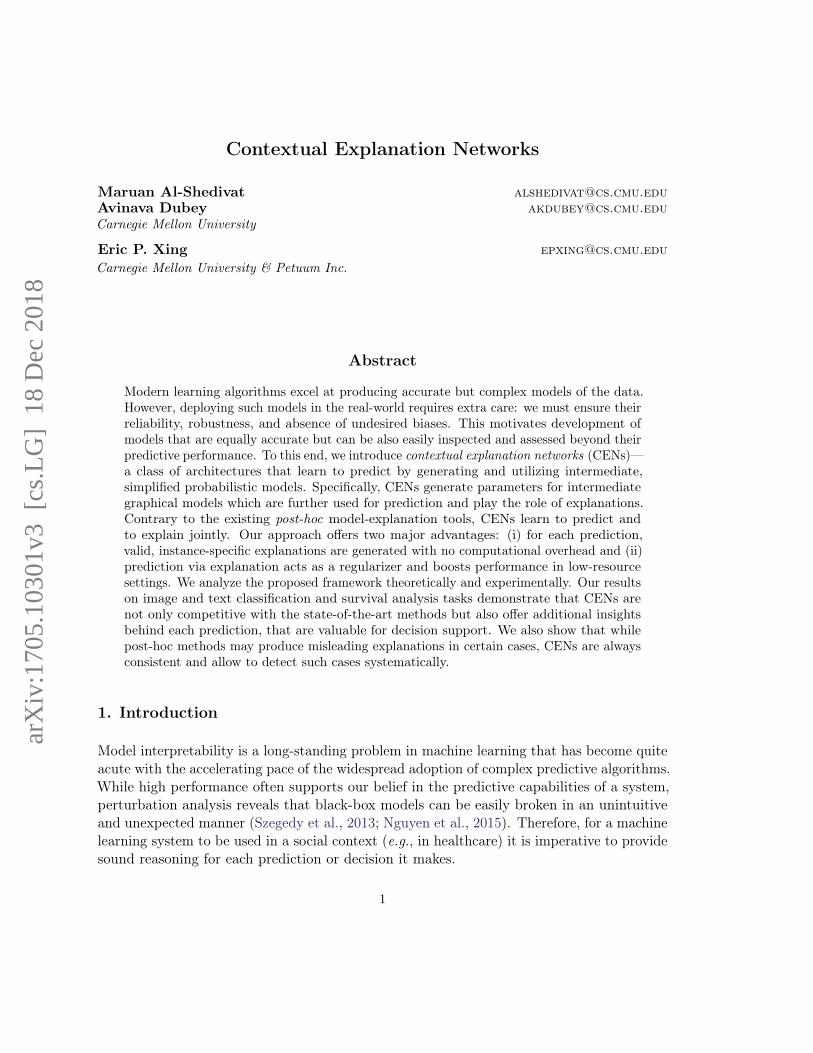
Figure 1: High-level functionality of CENs: The context is represented by satellite imagery and usedto generate instance-specific linear models (explanations). The latter act on a set of interpretableattributes from regional survey data and produce predictions.

To design such systems, we may restrict the class of models to only human-intelligible(Caruana et al., 2015). However, such an approach is often limiting in modern practicalsettings. Alternatively, we may fit a complex model and explain its predictions post-hoc, e.g.,by searching for linear local approximations of the decision boundary (Ribeiro et al., 2016).While such methods achieve their goal, explanations are generated a posteriori, requireadditional computation per data instance, and most importantly are never the basis for thepredictions made in the first place, which may lead to erroneous interpretations1.

Explanation is a fundamental part of the human learning and decision process (Lombrozo,2006). Inspired by this fact, we introduce contextual explanation networks (CENs)—a classof architectures that learn to predict and to explain jointly, alleviating the drawbacks ofthe post-hoc methods. To make a prediction, CENs operate as follows (Figure 1). First,they process a subset of inputs and generate parameters for a simple probabilistic model(e.g., sparse linear model) which is regarded interpretable by a domain expert. Then, thegenerated model is applied to another subset of inputs and produces a prediction. Tomotivate such an architecture, we consider the following example.

A motivating illustration. One of the tasks we consider in this paper is classificationof households into poor and not poor having access to satellite imagery and categorical datafrom surveys (Jean et al., 2016). If a human were to solve this task, to make predictions,they might assign weights to features in the categorical data and explain their predictions interms of the most relevant variables. Moreover, depending on the type of the area (based on

1. As we show in the paper, meaning and quality of generated explanations highly depends on the qualityof the features in terms of which predictions are explained. These so-called “interpretable features” areoften a matter of an arbitrary choice, but may significantly affect explanations produced post-hoc.

2


the available imagery), they might select slightly different weights for different areas (e.g.,when features indicative of poverty are different for urban and rural areas).

The CEN architecture given in Figure 1 imitates this process by learning an encoderthat maps images (the context) to parameters of sparse linear models which are furtherused for prediction. The learned encoder is sensitive to the infrastructure presented in theinput images and generates different linear models for urban and rural areas. The generatedmodels not only are used for prediction but also play the role of explanations and can encodearbitrary prior knowledge. CENs can represent complex model classes by using powerfulencoders. At the same time, by offsetting complexity into the encoding process, we achievesimplicity of explanations and can interpret predictions in terms the variables of interest.

The proposed architecture opens a number of questions: What are the fundamentaladvantages and limitations of CEN? How much of the performance should be attributed tothe context encoder and how much to the explanations? Are there any degenerate casesand do they happen in practice? Finally, how do CEN-generated explanations compare toalternatives, e.g., produced with LIME (Ribeiro et al., 2016)? In the sequel, we formalizeour intuitions and answer these questions theoretically and experimentally.

1.1 Contributions

The main four contributions of this paper are as follows:

(i) We formally define CENs as a class of probabilistic models, consider special cases, andderive learning and inference algorithms for scalar and structured outputs.

(ii) We design CENs in the form of new deep learning architectures trainable end-to-endfor prediction and survival analysis tasks.

(iii) Empirically, we demonstrate the value of learning with explanations for both predictionand model diagnostics. Moreover, we find that explanations can act as a regularizerand result in improved sample efficiency.

(iv) We also show that noisy features can render post-hoc explanations inconsistent andmisleading, and how CENs can help to detect and avoid such situations.

The code for reproducing experiments presented in this paper will be made publicly available.

1.2 Organization

The paper is organized as follows. Section 2 gives an overview of the related work. Section3 introduces our notation and some background on post-hoc interpretability methods. InSections 4, we introduce the general CEN framework, describe specific implementations,learning, and inference. In Section 5, we discuss and analyze properties of CEN theoretically.In Sections 6.1–6.2, we present experimental results for scalar prediction tasks and analyzeconsistency of linear explanations generated by CEN vs. alternatives. Finally, Section 6.3shows how CENs with structured explanations can efficiently solve survival analysis tasks.

3


C

θ

w

N

X

Y

(a)

C

θ

w

N

X1

Y1

X2

Y2

X3

Y3

(b)

C

θ

pq

N

X1

Y1

X2

Y2

X3

Y3

(c)

Figure 2: (a) A graphical model for CEN with a context encoder parameterized by w and linearexplanations. (b) A graphical model for CEN with context encoder and CRF-based explanations.The model is parameterized by w. (c) A graphical model for CEN with context autoencoding viathe inference, q, and generator, p, networks and CRF-based explanations.

2. Related work

Contextual explanation networks combine multiple threads of research that we discuss below.

2.1 Deep graphical models

The idea of combining deep networks with graphical models has been explored extensively.Notable threads of recent work include: replacing task-specific feature engineering withtask-agnostic general representations (or embeddings) discovered by deep networks (Col-lobert et al., 2011; Rudolph et al., 2016, 2017), representing energy functions (Belanger andMcCallum, 2016) and potential functions (Jaderberg et al., 2014) with neural networks,encoding learnable structure into Gaussian processes with deep and recurrent networks (Wil-son et al., 2016; Al-Shedivat et al., 2017), or learning state-space models on top of nonlinearembeddings of the observations (Gao et al., 2016; Johnson et al., 2016; Krishnan et al., 2017).The goal of this body of work is to design principled structured probabilistic models thatenjoy the flexibility of deep learning. The key difference between CENs and the previous artis that the latter directly integrate neural networks into graphical models as components(embeddings, potential functions, etc.). While flexible, the resulting deep graphical modelscould no longer be interpreted in terms of crisp relationships between specific variablesof interest2. CENs, on the other hand, preserve simplicity of the explanations and shiftcomplexity into conditioning on the context.

2. To see why this is the case, consider graphical models given in Figure 2 which relate input, X, and target,Y, variables using linear pairwise potential functions. Linearity allows to directly interpret parametersof the model as associations between the variables. Substituting inputs, X, with deep representationsor defining potentials via neural networks would result in a more powerful model. However, preciserelationships between the variables will be no longer directly readable from the model parameters.

4


2.2 Context representation

Generating probabilistic models after conditioning on a context is the key aspect of ourapproach. Previous work on context-specific graphical models represented contexts with adiscrete variable that enumerated a finite number of possible contexts (Koller and Friedman,2009, Ch. 5.3). CENs, on the other hand, are designed to handle arbitrary complex contextrepresentations. Context-specific approaches are widely used in language modeling wherethe context is typically represented with trainable embeddings (Rudolph et al., 2016). Wealso note that few-shot learning explicitly considers a setup where the context is representedby a small set of labeled examples (Santoro et al., 2016; Garnelo et al., 2018).

2.3 Meta-learning

The way CENs operate resembles the meta-learning setup. In meta-learning, the goal is tolearn a meta-model which, given a task, can produce another model capable of solving thetask (Thrun and Pratt, 1998). The representation of the task can be seen as the context whileproduced task-specific models are similar to CEN-generated explanations. Meta-training adeep network that generates parameters for another network has been successfully used forzero-shot (Lei Ba et al., 2015; Changpinyo et al., 2016) and few-shot (Edwards and Storkey,2016; Vinyals et al., 2016) learning, cold-start recommendations (Vartak et al., 2017), and afew other scenarios (Bertinetto et al., 2016; De Brabandere et al., 2016; Ha et al., 2016),but is not suitable for interpretability purposes. In contrast, CENs generate parametersfor models from a restricted class (potentially, based on domain knowledge) and use theattention mechanism (Xu et al., 2015) to further improve interpretability.

2.4 Model interpretability

While there are many ways to define interpretability (Lipton, 2016; Doshi-Velez and Kim,2017), our discussion focuses on explanations defined as simple models that locally approxi-mate behavior of a complex model. A few methods that allow to construct such explanationsin a post-hoc manner have been proposed recently (Ribeiro et al., 2016; Shrikumar et al.,2017; Lundberg and Lee, 2017), some of which we review in the next section. In contrast,CENs learn to generate such explanations along with predictions. There are multipleother complementary approaches to interpretability ranging from a variety of visualizationtechniques (Simonyan and Zisserman, 2014; Yosinski et al., 2015; Mahendran and Vedaldi,2015; Karpathy et al., 2015), to explanations by example (Caruana et al., 1999; Kim et al.,2014, 2016; Koh and Liang, 2017), to natural language rationales (Lei et al., 2016). Finally,our framework encompasses the so-called personalized or instance-specific models that learnto partition the space of inputs and fit local sub-models (Wang and Saligrama, 2012).

5


3. Background

We start by introducing the notation and reviewing post-hoc model explanations, with afocus on LIME (Ribeiro et al., 2016) as one of the most popular frameworks to date.

Given a collection of data where each instance is represented by inputs, c ∈ C, and targets,y ∈ Y , our goal is to learn an accurate predictive model, f : C 7→ Y . To explain predictions,we can assume that each data point has another set of features, x ∈ X . We constructexplanations in the form of simpler models, gc : X 7→ Y , so that they are consistent with theoriginal model in the neighborhood of the corresponding data instance, i.e., gc(x) = f(c).While the original inputs, c, can be of complex, low-level, unstructured data types (e.g.,text, image pixels, sensory inputs), we assume that x are high-level, meaningful variables(e.g., categorical features). In the post-hoc explanation literature, it is assumed that x arederived from c and are often binary (Lundberg and Lee, 2017) (e.g., c can be images, whilex can be vectors of binary indicators over the corresponding super-pixels). We consider amore general setup where c and x can be arbitrary, non-derivative modalities of the data.Throughout the paper, we call c the context and x the attributes or variables of interest.

Locally Interpretable Model-agnostic Explanations (LIME)

Given a trained model, f , and a data instance with features (c,x), LIME constructs anexplanation, gc, as follows:

gc = arg ming∈G

L(f, g, πc) + Ω(g) (1)

where L(f, g, πc) is the loss that measures how well g approximates f in the neighborhooddefined by the similarity kernel, πc : X 7→ R+, in the space of attributes, X , and Ω(g) isthe penalty on the complexity of explanation3. Now more specifically, Ribeiro et al. (2016)assume that G is the class of linear models, gc(x) := bc + wc · x, and define the loss and thesimilarity kernel as follows:

L(f, g, πc) :=∑x′∈X

πc(x′)(f(c′)− g(x′)

)2, πc(x′) := exp

−D(x,x′)2/σ2

(2)

where the data instance of interest is represented by (c,x), x′ and the corresponding c′ arethe perturbed features, D(x,x′) is some distance function, and σ is the scale parameter ofthe kernel. The regularizer, Ω(g), is often chosen to favor sparse explanations.

The model-agnostic property is the key advantage of LIME (and variations)—we cansolve (1) for any trained model, f , any class of explanations, G, at any point of interest,(c,x). While elegant, predictive and explanatory models in this framework are learnedindependently and hence never affect each other. In the next section, we propose a class ofmodels that ties prediction and explanation together in a joint probabilistic framework.

3. Ribeiro et al. (2016) argue that only simple models of low complexity (e.g., sufficiently sparse linearmodels) are human-interpretable and support that by human studies.

6


Dictionary

dot

Context

Context Encoder

Attention

C

Attributes

X

θ

X1 X2 X3 X4

Y1 Y2 Y3 Y4

Explanation

Figure 3: An example of CEN architecture. The context is represented by an image and transformedby a convnet encoder into an attention vector, which is used to construct a contextual hypothesisfrom a dictionary of sparse atoms.

4. Contextual Explanation Networks

We consider the same problem of learning from a collection of data represented by contextvariables, c ∈ C, attributes, x ∈ X , and targets, y ∈ Y. We denote the correspondingrandom variables by capital letters, C, X, and Y, respectively. Our goal is to learn a model,Pw (Y | x, c), parametrized by w that can predict y from x and c. We define contextualexplanation networks as probabilistic models that assume the following form4 (Figure 2):

y ∼ P (Y | x,θ) , θ ∼ Pw (θ | c) , Pw (Y | x, c) =

∫P (Y | x,θ)Pw (θ | c) dθ (3)

where P (Y | x,θ) is a predictor parametrized by θ. We call such predictors explanations,since they explicitly relate interpretable attributes, x, to the targets, y. For example, whenthe targets are scalar and binary, explanations may take the form of linear logistic models;when the targets are more complex, dependencies between the components of y can berepresented by a graphical model, e.g., conditional random field (Lafferty et al., 2001).

CENs assume that each explanation is context-specific: Pw (θ | c) defines a conditionalprobability of an explanation θ being valid in the context c. To make a prediction, wemarginalize out θ. To interpret a prediction, y, for a given data instance, (x, c), we inferthe posterior, Pw (θ | y,x, c). The main advantage of this approach is to allow modelingconditional probabilities, Pw (θ | c), in a black-box fashion while keeping the class ofexplanations, P (Y | x,θ), simple and interpretable. For instance, when the context is givenas raw text, we may choose Pw (θ | c) to be represented with a recurrent neural network,while P (Y | x,θ) be in the class of linear models.

Implications of these assumptions are discussed in Section 5. Here, we continue with adiscussion of a number of practical choices for Pw (θ | c) and P (Y | x,θ) (Table 1).

4. While we focus on predictive modeling, CENs are applicable beyond that. For example, instead oflearning a predictive distribution, Pw (Y | x, c), we may want to learn a contextual marginal distribution,Pw (X | c), over a set random variables X, where P (X | θ) is defined by an arbitrary graphical model.

7


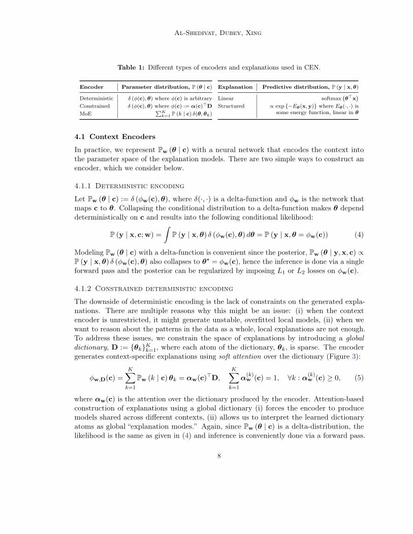
Table 1: Different types of encoders and explanations used in CEN.

Encoder Parameter distribution, P (θ | c)

Deterministic δ (φ(c),θ) where φ(c) is arbitraryConstrained δ (φ(c),θ) where φ(c) := α(c)>D

MoE∑K

k=1 P (k | c) δ(θ,θk)

Explanation Predictive distribution, P (y | x,θ)

Linear softmax(θ>x

)Structured ∝ exp −Eθ(x,y) where Eθ(·, ·) is

some energy function, linear in θ

4.1 Context Encoders

In practice, we represent Pw (θ | c) with a neural network that encodes the context intothe parameter space of the explanation models. There are two simple ways to construct anencoder, which we consider below.

4.1.1 Deterministic encoding

Let Pw (θ | c) := δ (φw(c),θ), where δ(·, ·) is a delta-function and φw is the network thatmaps c to θ. Collapsing the conditional distribution to a delta-function makes θ dependdeterministically on c and results into the following conditional likelihood:

P (y | x, c; w) =

∫P (y | x,θ) δ (φw(c),θ) dθ = P (y | x,θ = φw(c)) (4)

Modeling Pw (θ | c) with a delta-function is convenient since the posterior, Pw (θ | y,x, c) ∝P (y | x,θ) δ (φw(c),θ) also collapses to θ? = φw(c), hence the inference is done via a singleforward pass and the posterior can be regularized by imposing L1 or L2 losses on φw(c).

4.1.2 Constrained deterministic encoding

The downside of deterministic encoding is the lack of constraints on the generated expla-nations. There are multiple reasons why this might be an issue: (i) when the contextencoder is unrestricted, it might generate unstable, overfitted local models, (ii) when wewant to reason about the patterns in the data as a whole, local explanations are not enough.To address these issues, we constrain the space of explanations by introducing a globaldictionary, D := θkKk=1, where each atom of the dictionary, θk, is sparse. The encodergenerates context-specific explanations using soft attention over the dictionary (Figure 3):

φw,D(c) =K∑k=1

Pw (k | c)θk = αw(c)>D,K∑k=1

α(k)w (c) = 1, ∀k : α

(k)w (c) ≥ 0, (5)

where αw(c) is the attention over the dictionary produced by the encoder. Attention-basedconstruction of explanations using a global dictionary (i) forces the encoder to producemodels shared across different contexts, (ii) allows us to interpret the learned dictionaryatoms as global “explanation modes.” Again, since Pw (θ | c) is a delta-distribution, thelikelihood is the same as given in (4) and inference is conveniently done via a forward pass.

8


The two proposed context encoders represent P (θ | c) with delta-functions, whichsimplifies learning, inference, and interpretation of the model, and are used in our experiments.Other ways to represent P (θ | c) include: (i) using a mixture of delta-functions (which makesCEN function similar to a mixture-of-experts model and further discussed in Section 5.1), or(ii) using variational autoencoding. We leave more complex approaches to future research.

4.2 Explanations

In this paper, we consider two types of explanations: linear that can be used for regressionor classification and structured that are suitable for structured prediction.

4.2.1 Linear Explanations

In case of classification, CENs with linear explanations assume the following P (Y | x,θ):

P (Y = i | x,θ) :=exp (Wx + b)i∑j∈Y exp (Wx + b)j

, (6)

where θ := (W,b) and i, j index classes in Y . If x is d-dimensional and we are given m-classclassification problem, then W ∈ Rm×d and b ∈ Rm. The case of regression is similar.

In Section 5.4, we show that if we apply LIME to interpret CEN with linear explanations,the local linear models inferred by LIME are guaranteed to recover the original CEN-generated explanations. In other words, linear explanations generated by CEN have similarproperties, e.g., local faithfulness (Ribeiro et al., 2016). However, we emphasize the keydifference between LIME and CEN: the former regards explanation as a post-processingstep (done after training) while the latter integrates explanation into the learning process.

4.2.2 Structured Explanations

While post-hoc methods, such as LIME, can easily generate local linear explanations forscalar outputs, using such methods for structured outputs is non-trivial. At the same time,CENs let us represent P (Y | x,θ) using arbitrary graphical models. To be concrete, weconsider the case where the targets are binary vectors, y ∈ 0, 1m, and explanations arerepresented by CRFs (Lafferty et al., 2001) with linear potential functions.

The predictive distribution P (Y | x,θ) represented by a CRF takes the following form:

P (Y | x,θ) :=1

Zθ(x)

∏a∈A

Ψa(ya,xa;θ) (7)

where Zθ(x) is the normalizing constant and a ∈ A indexes subsets of variables in x and ythat correspond to the factors:

Ψa(ya,xa;θ) := exp

K∑k=1

θakfak(xa,ya)

, (8)

9


where fak(xa,ya)Kk=1 is a collection of feature vectors associated with factor Ψa(ya,xa;θ).For interpretability purposes, we are interested in CRFs with feature vectors that are linearor bi-linear in x and y. There is a variety of application-specific CRF models developedin the literature (e.g., see Sutton et al., 2012). While in the following section, we discusslearning and inference more generally, in Section 6.3 we develop a CEN model with linearchain CRF explanations for solving survival analysis tasks.

4.3 Inference and Learning

CENs with deterministic encoders are convenient since the posterior, P (θ | y,x, c), collapsesto a point θ? = φ(c). Inference in such models is done in two steps: (1) first, compute θ?,then (2) using θ? as parameters, compute the predictive distribution, P (y | x,θ?). To trainthe model, we can optimize its log likelihood on the training data. To make a predictionusing a trained CEN model, we infer y = arg maxy P (y | x,θ?). For classification (andregression) computing predictions is straightforward. Below, we show how to computepredictions for CEN with CRF-based explanations.

4.3.1 Inference for CEN with Structured Explanations

Given a CRF model (7), we can make a prediction y for inputs (c,x) by performing inference:

y(θ?) = arg maxy∈Y

P (y | x,θ?) = arg maxy∈Y

A∑a=1

K∑k=1

θ?akfak(xa,ya) (9)

Depending on the structure of the CRF model (e.g., linear chain, tree-structured model,etc.), we could use different inference algorithms, such the Viterbi algorithm or variationalinference, in order to solve (9) (see Ch. 4, Sutton et al., 2012, for an overview and examples).The key point here is that having P (y | x,θ?) or y(θ?) computable in an (approximate)functional form, lets us construct different objective functions, e.g., L(yi,xi, ciNi=1,w),and learn parameters of the CEN model end-to-end using gradient methods, which arestandard in deep learning. In Section 6.3, we construct a specific objective function forsurvival analysis.

4.3.2 Learning via Likelihood Maximization and Posterior Regularization

In this paper, we use the negative log likelihood (NLL) objective for learning CEN models:

L(yi,xi, ciNi=1,w) :=1

N

N∑i=1

logP (yi | xi,θ = φw(ci)) (10)

L1, L2, and other types of regularization imposed on θ can be added to the objective (10).Such regularizers, as well as the dictionary constraint introduced in Section 4.1.2, can beseen as a form of posterior regularization (Ganchev et al., 2010) and are important forachieving the best performance and interpretability.

10


5. Analysis

In this section, we dive into the analysis of CEN as a class of probabilistic models. First,we mention special cases of CEN model class known in the literature, such as mixture-of-experts (Jacobs et al., 1991) and varying-coefficient models (Hastie and Tibshirani, 1993).Then, we discuss implications of the CEN structure, a potential failure mode of CEN withdeterministic encoders and how to rectify it using conditional entropy regularization, andfinally analyze relationship between CEN-generated and post-hoc explanations. Readerswho are mostly interested in empirical properties and applications may skip this section.

5.1 Special Cases of CEN

Mixtures of Experts. So far, we have represented Pw (θ | c) by a delta-function centeredaround the output of the encoder. It is natural to extend Pw (θ | c) to a mixture of delta-distributions, in which case CENs recover the mixtures-of-experts model (MoE, Jacobset al., 1991). To see this, let D be a dictionary of experts, and define Pw,D (θ | c) :=∑K

k=1 Pw (k | c) δ(θ,θk). The log-likelihood for CEN in such case is the same as for MoE:

X1 X2 X3 X4

Y1 Y2 Y3 Y4

Y1 Y2 Y3 Y4

X1 X2 X3 X4

Y1 Y2 Y3 Y4

X1 X2 X3 X4

Y1 Y2 Y3 Y4

Mixture of Experts

dotAttention

logPw,D (yi | xi, ci)

= log

∫P (yi|xi,θ)Pw,D (θ|ci) dθ

= log

K∑k=1

Pw (k|ci)P (yi|xi,θk)

(11)

As in Section 4.1.2, Pw (k | C) is represented with a soft attention over the dictionary, D,which is now used to combine predictions of the experts with parameters θkKk=1 insteadof constructing a single context-specific explanation. Learning of MoE models is done eitherby optimizing the likelihood or via expectation maximization (EM). Note another differencebetween CEN and MoE is that the latter assumed that c ≡ x and that both P (y | x,θ) andP (θ | c) can be represented by arbitrary complex model classes, ignoring interpretability.Varying-Coefficient Models. In statistics, there is a class of (generalized) regressionmodels, called varying-coefficient models (VCMs, Hastie and Tibshirani, 1993), in whichcoefficients of linear models are allowed to be smooth deterministic functions of othervariables (called the “effect modifiers”). Interestingly, the motivation for VCM was toincrease flexibility of linear regression. In the original work, Hastie and Tibshirani (1993)focused on simple dynamic (temporal) linear models and on nonparametric estimation ofthe varying coefficients, where each coefficient depended on a different effect variable. CENgeneralizes VCM by (i) allowing parameters, θ, to be random variables that depend on thecontext, c, nondeterministically, (ii) letting the “effect modifiers” to be high-dimensionalcontext variables (not just scalars), and (iii) modeling the effects using deep neural networks.In other words, CEN alleviates the limitations of VCM by leveraging the probabilisticgraphical models and deep learning frameworks.

11


5.2 Implications of the structure of CENs

CENs represent the predictive distribution in a compound form (Lindsay, 1995):

P (Y | X,C) =

∫P (Y | X,θ)P (θ | C) dθ

and we assume that the data is generated according to Y ∼ P (Y | X,θ), θ ∼ P (θ | C).We would like to understand:

Can CEN represent any conditional distribution, P (Y | X,C), when theclass of explanations is limited ( e.g., to linear models)? If not, what are thelimitations?

Generally, CEN can be seen as a mixture of predictors. Such mixture models could be quitepowerful as long as the mixing distribution, P (θ | C), is rich enough. In fact, even a finitemixture exponential family regression models can approximate any smooth d-dimensionaldensity at a rate O(m−4/d) in the KL-distance (Jiang and Tanner, 1999). This resultsuggests that representing the predictive distribution with contextual mixtures should notlimit the representational power of the model. However, there are two caveats:

(i) In practice, P (θ | C) is limited, since we represent it either with a delta-function, afinite mixture, or a simple distribution parametrized by a deep network.

(ii) Classical predictive mixtures (including MoE) do not separate input features into twosubsets, c and x. We do this intentionally to produce explanations in terms of specificvariables of interest that could be useful for interpretability or model diagnostics downthe line. However, it could be the case that x contains only some limited informationabout y, which could limit the predictive power of the full model.

To address point (i), we consider P (θ | c) that fully factorizes over the dimensions of θ:P (θ | c) =

∏j P (θj | c), and assume that explanations, P (Y | x,θ), also factorize according

to some underlying graph, GY = (VY, EY). The following proposition shows that in suchcase P (Y | x, c) inherits the factorization properties of the explanation class.

Proposition 1 Let P (θ | c) :=∏j P (θj | c) and let P (Y | x,θ) factorize according to

some graph GY = (VY, EY). Then, P (Y | x, c) defined by CEN with P (θ | c) encoder andP (Y | x,θ) explanations also factorizes according to G.Proof The statement directly follows from the definition of CEN (see Appendix A.1).

Remark 2 All encoders, P (θ | c), considered in this paper, including delta functions andtheir mixtures, fully factorize over the dimensions of θ.

Remark 3 The proposition has no implications for the case of scalar targets, y. However,in case of structured prediction, regardless of how good the context encoder is, CEN willstrictly assume the same set of independencies as given by the explanation class, P (Y | x,θ).

12


As indicated in point (ii), CENs assume a fixed split of the input features into context, c,and variables of interest, x, which has interesting implications. Ideally, we would like x tobe a good predictor of y in any context c. For instance, following our motivation example(see Figure 1), if c distinguishes between urban and rural areas, x must encode enoughinformation for predicting poverty within urban or rural neighborhoods. However, since thevariables of interest are often manually selected (e.g., by a domain expert) and limited, wemay encounter the following (not mutually exclusive) situations:

(a) c may happen to be a strong predictor of y and already contain information availablein x (e.g., it is the case when x is derived from c).

(b) x may happen to be a poor predictor of y, even within the context specified by c.

In both cases, CEN may learn to ignore x, leading to essentially meaningless explanations.In the next section, we show that, if (a) is the case, regularization can help eliminate suchbehavior. Additionally, if (b) is the case, i.e., x are bad features for predicting y (and forseeking explanation in terms of these features), CEN must indicate that. It turns out thatthe accuracy of CEN depends on the quality of x, as empirically shown in Section 6.2.2.

5.3 Conditional Entropy Regularization

CEN has a failure mode: when the context c is highly predictive of the targets y and theencoder is represented by a powerful model, CEN may learn to rely entirely on the contextvariables. In such case, the encoder would generate spurious explanations, one for eachtarget class. For example, for binary targets, y ∈ 0, 1, CEN may learn to always mapc to either θ0 or θ1 when y is 0 or 1, respectively. In other words, θ (as a function of c)would become highly predictive of y on its own, and hence P (Y | x,θ) ≈ P (Y | θ), i.e., Ywould be (approximately) conditionally independent of X given θ. This is problematic fromthe interpretation point of view since explanations would become spurious, i.e., no longerused to make predictions from the variables of interest.

Note that such a model would be accurate only when the generated θ is always highlypredictive of Y, i.e., when the conditional entropy H(Y | θ) is low. Following thisobservation, we propose to regularize the model by approximately maximizing H(Y | θ).For a CEN with a deterministic encoder (Sections 4.1.1 and 4.1.2), we can compute anunbiased estimate of H(Y | θ) given a mini-batch of samples from the dataset as follows:

H(Y | θ) =

∫P (y,θ) logP (y | θ) dydθ (12)

= E(c,x)∼P(c,x)

[∫P (y | x, φ(c)) logEx′∼P(x)

[P(y | x′, φ(c)

)]dy

](13)

≈ 1

|B|∑i∈B

∫P (y | xi, φ(ci)) log

1

|B|∑j∈B

P (y | xj , φ(ci))

dy (14)

13


C1

C2

C3

C4

X1X2

(a)

C1

C2

C3

C4

X1X2

(b)

Figure 4: A toy synthetic dataset and two linear explanations (green and orange) produced by aCEN model trained (a) with no regularization or (b) with conditional entropy regularization.

In the given expressions, elements of B index training samples (e.g., B represents a mini-batch), (13) is obtained by using the definition of CEN and marginalizing out θ, (14) is astochastic estimate that approximates expectations with a mini-batch of samples. Intuitively,if the predictions are accurate while H(Y | θ) is high, we can be sure that CEN learnedto generate contextual θ’s that are uncorrelated with the targets but result into accurateconditional models, P (Y | x,θ).

An illustration on synthetic data. To illustrate the problem, we consider a toy synthetic3D dataset with 2 classes that are not separable linearly (Figure 4). The coordinates alongthe vertical axis C correspond to different contexts, and (X1, X2) represent variables ofinterest. Note we can perfectly distinguish between the two classes by using only thecontext information. CEN with a dictionary of size 2 learns to select one of the two linearexplanations for each of the contexts. When trained without regularization (Figure 4a),selected explanations are spurious hyperplanes since each of them is used for points of asingle class only. Adding entropy regularization (Figure 4b) makes CEN select hyperplanesthat meaningfully distinguish between the classes within different contexts.

Quantifying contribution of the explanations. Starting from the introduction, wehave argued that explanations are meaningful when they are used for prediction. In otherwords, we would like explanations have a non-zero contribution to the overall accuracy of themodel. The following theorem quantifies the contribution of explanations to the predictiveperformance of entropy-regularized CEN.

14


Proposition 4 Let CEN with linear explanations have the expected predictive accuracy

EX,θ∼P(X,θ)

[P(Y = Y | X,θ

)]≥ 1− ε, (15)

where ε ∈ (0, 1) is small. Let also the conditional entropy be H(Y | θ) ≥ δ for some δ ≥ 0.Then, the expected contribution of the explanations to the predictive performance of CEN isgiven by the following lower bound:

EX,θ∼P(X,θ)

[P(Y = Y | X,θ

)− P

(Y = Y | θ

)]≥ δ − 1

log |Y| − ε, (16)

where |Y| denotes the cardinality of the target space.

Proof The statement follows from Fano’s inequality. For details, see Appendix A.2.

Remark 5 The proposition states that explanations are meaningful (as contextual models)only when CEN is accurate ( i.e., the expected predictive error is less than ε) and theconditional entropy H(Y | θ) is high. High accuracy and low entropy imply spuriousexplanations. Low accuracy and high entropy imply that x features are not predictive of ywithin the class of explanations, suggesting to reconsider our modeling assumptions.

5.4 CEN-generated vs. Post-hoc Explanations

In this section, we analyze the relationship between CEN-generated and LIME-generatedpost-hoc explanations. Given a trained CEN, we can use LIME to approximate its decisionboundary and compare the explanations produced by both methods. The question we ask:

How does the local approximation, θ, relate to the actual explanation, θ?,generated and used by CEN to make a prediction in the first place?

For the case of binary5 classification, it turns out that when the context encoder is determin-istic and the space of explanations is linear, local approximations, θ, obtained by solving(1) recover the original CEN-generated explanations, θ?. Formally, our result is stated inthe following theorem.

Theorem 6 Let the explanations and the local approximations be in the class of lin-ear models, P (Y = 1 | x,θ) ∝ exp

x>θ

. Further, let the encoder be L-Lipschitz and

pick a sampling distribution, πx,c, that concentrates around the point (x, c), such thatPπx,c (‖z′ − z‖ > t) < ε(t), where z := (x, c) and ε(t) → 0 as t → ∞. Then, if the lossfunction is defined as

L =1

K

K∑k=1

(logit P (Y = 1 | xk, ck) − logit P (Y = 1 | xk,θ))2 , (xk, ck) ∼ πx,c, (17)

the solution of (1) concentrates around θ? as Pπx,c(‖θ − θ?‖ > t

)≤ δK,L(t), δK,L −→

t→∞0.

5. Analysis of the multi-class case can be reduced to the binary in the one-vs-all fashion.

15


Intuitively, by sampling from a distribution sharply concentrated around (x, c), we ensurethat θ will recover θ? with high probability.

This result establishes an equivalence between the explanations generated by CEN andthose produced by LIME post-hoc when approximating CEN. Note that when LIME isapplied to a model other than CEN, equivalence between explanations is not guaranteed.Moreover, as we further show experimentally, certain conditions such as incomplete or noisyinterpretable features may lead to LIME producing inconsistent and erroneous explanations.The proof of the theorem is given in Appendix A.3.

6. Case Studies

In this section, we move to a number of case studies where we empirically analyze propertiesof the proposed CEN framework on classification and survival analysis tasks. In particular,we evaluate CEN with linear explanations on a few classification tasks that involve differentdata modalities of the context (e.g., images or text). For survival prediction, we design CENarchitectures with structured explanations, derive learning and inference algorithms, andshowcase our models on problems from the healthcare domain.

6.1 Solving Classification using CEN with Linear Explanations

We start by examining the properties of CEN with linear explanations (Table 1) on a fewclassification tasks. Our experiments are designed to answer the following questions:

(i) When explanation is a part of the learning and prediction process, how does that affectperformance of the final predictive model quantitatively?

(ii) Qualitatively, what kind of insight can we gain by inspecting explanations?(iii) Finally, we analyze consistency of linear explanations generated by CEN versus those

generated using LIME (Ribeiro et al., 2016), a popular post-hoc method.

Details on our experimental setup, all hyperparameters, and training procedures are givenin the tables in Appendix B.3.

6.1.1 Poverty Prediction

We consider the problem of poverty prediction for household clusters in Uganda from satelliteimagery and survey data. Each household cluster is represented by a collection of 400× 400satellite images (used as the context) and 65 categorical variables from living standardsmeasurement survey (used as the interpretable attributes). The task is binary classificationof the households into poor and not poor.

We follow the original study of Jean et al. (2016) and use a VGG-F network (pre-trainedon nightlight intensity prediction) to compute 4096-dimensional embeddings of the satelliteimages on top of which we build contextual models. Note that this datasets is fairly small(500/142 train/test points), and so we keep the VGG-F part frozen to avoid overfitting.

16


M1 M2

Water: Unreliable

Water src: Public tap

Walls: Unburnt bricks

Roof: Thatch, Straw

Is water payed

Vegetation

Has electricity

Nightlight intensity

0.9 -0.4

-0.6 -1.2

0.3 -0.2

0.5 0.2

-0.3 -0.3

-0.1 0.4

-0.2 -0.8

-0.7 -0.7

−0.8

−0.4

0.0

0.4

0.8

(a)

0.3

0.4

0.5

0.6

0.7

Tim

esm

odel

sele

cted

(%)

M1

M2

Rural Urban0.1

0.2

0.3

0.4H

Hty

pe:

Ten

emen

t(%

)M1

M2

(b)

Arua

Gulu

Kampala (capital)

Iganga

Masaka

Kasese

Uganda: Contextual Models

M1

M2

(c)

Arua

Gulu

Kampala (capital)

Iganga

Masaka

Kasese

Uganda: Nightlight Intensity

0%

100%

(d)

Figure 5: Qualitative results for the Satellite dataset: (a) Weights given to a subset of features bythe two models (M1 and M2) discovered by CEN. (b) How frequently M1 and M2 are selected forareas marked rural or urban (top) and the average proportion of Tenement-type households in anurban/rural area for which M1 or M2 was selected. (c) M1 and M2 models selected for differentareas on the Uganda map. M1 tends to be selected for more urbanized areas while M2 is picked forthe rest. (d) Nightlight intensity of different areas of Uganda.

Table 2: Performance of themodels on the poverty prediction.

Acc (%) AUC (%)

LRemb 62.5% 68.1

LRatt 75.7% 82.2

MLP 77.4% 78.7

MoEatt 77.9% 85.4

CENatt 81.5% 84.2

Models. For baselines, we use logistic regression (LR)and multi-layer perceptrons (MLP) with 1 hidden layer.The LR baseline uses either VGG-F embeddings (LRemb) orthe categorical attributes (LRatt) as inputs. The input ofthe MLP baseline is concatenated VGG-F embeddings andcategorical attributes. Context encoder of the CEN modeluses VGG-F to process images, followed by an attention layerover a dictionary of 16 trainable linear explanations definedover the categorical features (Figure 3). Finally, we evaluatea mixture-of-experts (MoE) model of the same architectureas CEN, since it is a special case (see Section 5.1). BothCEN and MoE are trained with the dictionary constraint and L1 regularization to encouragesparse explanations. Details on the architectures and training are given in Table 7b.

Performance. The results are presented in Table 2. Both in terms of accuracy and AUC,CEN models outperform both simple logistic regression and vanilla MLP. Even thoughthe results suggest that categorical features are better predictors of poverty than VGG-Fembeddings of images, note that using embeddings to contextualize linear models reducesthe error. This indicates that different linear models are optimal in different contexts.

Qualitative analysis. We discovered that, on this task, CEN encoder tends to sharplyselect one of the two explanations (M1 and M2) for different household clusters in Uganda(Figure 5a). In the survey data, each household cluster is marked as either urban or rural.We notice that, conditional on a satellite image, CEN tends to pick M1 for urban areas andM2 for rural (Figure 5b). Notice that different explanations weigh categorical features, such

17


Table 3: Sentiment classification error rate on IMDB dataset. It is interesting to note that CENsgets state of the art performance by only using supervised data (25 thousand labeled reviews) whileMiyato et al. (2016) obtain their result by using additional 50K unlabelled reviews.

Method Reference Error

BoW (bnc) Maas et al. (2011a) 12.20%BoW (b∆tc) Maas et al. (2011a) 11.77%LDA Maas et al. (2011a) 32.58%Full + BoW Maas et al. (2011a) 11.67%Full + Unlabelled + BoW Maas et al. (2011a) 11.11%WRRBM Dahl et al. (2012) 12.58%WRRBM + BoW Dahl et al. (2012) 10.77%MNB-uni Wang and Manning (2012) 16.45%MNB-bi Wang and Manning (2012) 13.41%SVM-uni Wang and Manning (2012) 13.05%SVM-bi Wang and Manning (2012) 10.84%NBSVM-uni Wang and Manning (2012) 11.71%NBSVM-bi Wang and Manning (2012) 8.78%NBSVM-bi Wang and Manning (2012) 8.78%seq2-brown-CNN Johnson and Zhang (2014) 14.70%Paragraph Vector Le and Mikolov (2014) 7.42%SA-LSTM with joint training Dai and Le (2015) 14.70%LSTM with tuning and dropout Dai and Le (2015) 13.50%LSTM initialized with word2vec embeddings Dai and Le (2015) 10.00%SA-LSTM with linear gain Dai and Le (2015) 9.17%LM-TM Dai and Le (2015) 7.64%SA-LSTM Dai and Le (2015) 7.24%Virtual Adversarial Miyato et al. (2016) 5.94 ± 0.12%TopicRNN Dieng et al. (2017) 6.28%

CEN-bow 5.92 ± 0.05 %CEN-tpc 6.25 ± 0.09 %

as reliability of the water source or the proportion of houses with walls made of unburntbrick, quite differently. When visualized on the map, we see that CEN selects M1 morefrequently around the major city areas, which also correlates with high nightlight intensityin those areas (Figures 5c,5d). We also estimate the approximate conditional entropy of thebinary targets (poor vs. not poor) given the selected model and find: H(Y | θ = M1) ≈ 77%and H(Y | θ = M2) ≈ 72%. High performance of the model along with high conditionalentropy makes us confident in the produced explanations (see Section 5.3) and allows usto draw conclusions about what causes the model to classify certain households in differentneighborhoods as poor in terms of interpretable categorical variables.

18


−5 0 5

102

103

Bad acting/plot:[’script’, ’acting’, ’bad’, ’plot’, ’film’]

−5 0 5

Great story/performance:[’great’, ’story’, ’film’, ’brilliant’]

−5 0 5

A movie one has seen:[’just’, ’movie’, ’watched’, ’good’]

0.000 0.001

101

103

Bollywood movies:[’bollywood’, ’indian’, ’action’, ’kumar’]

0.000 0.001 0.002

Soap operas:[’italian’, ’soap’, ’russian’, ’opera’]

−0.0005 0.0000 0.0005

Art/nature movies:[’art’, ’earth’, ’nature’, ’jungle’]

Figure 6: Histograms of test weights assigned by CEN to 6 topics: acting- and plot-related topics(upper charts), genre topics (bottom charts).

6.1.2 Sentiment Analysis

The next problem we consider is sentiment prediction of IMDB reviews (Maas et al., 2011b).The reviews are given in the form of English text (sequences of words) and the sentimentlabels are binary (good/bad movie). This dataset has 25k labelled reviews used for trainingand validation and 25k labelled reviews that are held out for test. The data also containsan additional set of 50k unlabelled reviews that are used by some models in the literature.We emphasize that we do not use the unlabelled part of the data for training CENs.

Models. Following Johnson and Zhang (2016), we use a bi-directional LSTM with max-pooling as our baseline that predicts sentiment directly from text sequences. The samearchitecture is used as the context encoder in CEN that produces parameters for linearexplanations. The explanations are applied to either (a) a bag-of-words (BoW) features(with a vocabulary limited to 5,000 most frequent words) or (b) a 100-dimensional topicrepresentation produced by a separately trained off-the-shelf topic model (Blei et al., 2003).

Performance. Comparison of CEN with other models from the literature is given inTable 3. Not only CEN achieves a near state-of-the-art accuracy on this dataset, weemphasize that we do not use any unlabeled data when training our models. This indicatesthat the inductive biases provided by the architecture lead to a more significant performanceimprovement that many of the semi-supervised training methods on this dataset.

19


Table 4: Prediction error of the models on image classification tasks (averaged over 5 runs; thestd. are on the order of the least significant digit). The subscripts denote the features on which thelinear models are built: pixels (pxl), HOG (hog).

MNIST CIFAR10

LRpxl LRhog CNN MoEpxl MoEhog CENpxl CENhog LRpxl LRhog VGG MoEpxl MoEhog CENpxl CENhog

8.00 2.98 0.75 1.23 1.10 0.76 0.73 60.1 48.6 9.4 13.0 11.7 9.6 9.2

Qualitative analysis. After training CEN-tpc with linear explanations in terms of topicson the IMDB dataset, we generate explanations for each test example and visualize histogramsof the weights assigned by the explanations to the 6 selected topics in Figure 6. The 3topics in the top row are acting- and plot-related (and intuitively have positive, negative,or neutral connotation), while the 3 topics in the bottom are related to particular genre ofthe movies. Note that acting-related topics turn out to be bimodal, i.e., contributing eitherpositively, negatively, or neutrally to the sentiment prediction in different contexts. CENassigns a high negative weight to the topic related to “bad acting/plot” and a high positiveweight to “great story/performance” in most of the contexts (and treats those neutrallyconditional on some of the reviews). Interestingly, genre-related topics almost always have anegligible contribution to the sentiment which indicates that the learned model does nothave any particular bias towards or against a given genre.

Figure 14 in Appendix visualizes the full dictionary of size 16 learned by CEN-tpc. Eachcolumn corresponds to a dictionary atom that represents a typical explanation patternthat CEN attends to before making a prediction. By inspecting the dictionary, we canfind interesting patterns. For instance, atoms 5 and 11 assign inverse weights to thefollowing topics denoted by the top 4 words: [kid, child, disney, family] and [sexual,violence, nudity, sex] (i.e., good family movies must not be violent and vice versa).Depending on the context of the review, CEN may select one of these patterns to predictthe sentiment. Note that these two topics are negatively correlated across all dictionaryelements, which again is quite intuitive.

6.1.3 Image Classification

For the purpose of completeness, we also provide results on two classical image datasets:MNIST and CIFAR-10. For CEN, full images are used as the context; to imitate high-levelfeatures, we use (a) the original images cubically downscaled to 20× 20 pixels, gray-scaledand normalized, and (b) HOG descriptors computed using 3× 3 blocks (Dalal and Triggs,2005). For each task, we use linear regression and vanilla convolutional networks as baselines(a small convnet for MNIST and VGG-16 for CIFAR-10). The results are reported in Table 4.CENs are competitive with the baselines and do not exhibit deterioration in performance.Visualization and analysis of the learned explanations is given in Appendix B.2 and thedetails on the architectures, hyperparameters, and training are given in Appendix B.3

20


1 4 42 43 44 45

Dictionary size

0

2

4

6

Valid

atio

ner

ror(

%)

MNIST

CNNCEN-pxlCEN-hog

1 4 42 43 44 45

Dictionary size

0

10

20

30IMDB

LSTMCEN-bowCEN-tpc

(a)

0 10 20

Epoch number

0.25

0.5

1.0

Trai

ner

ror(

%)

MNIST

CNNCEN-pxlCEN-hog

0 500 1000

Batch number

20

40

60IMDB

LSTMCEN-tpc

(b)

0 5 10 15Train set size (%)

0

5

10

Test

erro

r(%

)

MNIST

CNNCEN-pxlCEN-hog

0 10 20 30 40Train set size (%)

0

10

20

30

40IMDB

LSTMCEN-bowCEN-tpc

(c)

Figure 7: (a) Validation error vs. dictionary size. (b) Training error vs. iteration (epoch or batch)for baselines and CEN. (c) Test error for models trained on random subsets of data of different sizes.

6.2 Properties of Explanations

In this section, we look at the explanations from the regularization and consistency pointof view. As we show next, prediction via explanation not only has a strong regularizationeffect, but also always produces consistent locally linear models.

6.2.1 Explanations as a Regularizer

By controlling the dictionary size, we can control the expressivity of the model class specifiedby CEN. For example, when the dictionary size is 1, CEN becomes equivalent to a linearmodel. For larger dictionaries, CEN becomes as flexible as a deep network (Figure 7a).Adding a small sparsity penalty to each element of the dictionary (between 10−6 and 10−3,see Appendix B.3) helps to avoid overfitting for very large dictionary sizes, so that the modellearns to use only a few dictionary atoms for prediction while shrinking the rest to zero.

If explanations can act as a proper regularizer, we must observe improved samplecomplexity of the model. To verify this, we trained CEN models on subsets of data (sizevaried between 1% and 20% for MNIST and 2% and 40% for IMDB) and then evaluatedaccuracy on the validation set. As seen from the error reported in Figure 7c, CENs requiremuch fewer samples to attain a near top accuracy (as if trained on the full dataset). Finally,we also observe that CEN models tend to converge faster (Figure 7b) which indicates thatprediction via explanation improves the geometry of the optimization problem.

6.2.2 Consistency of Explanations

While regularization is a useful aspect, the main use case for explanations is model diagnostics.Linear explanations assign weights to the interpretable features, X, and hence their qualitydepends on the way we select these features. In this section, we evaluate explanationsgenerated by CEN or a post-hoc method (LIME). In particular, we consider two caseswhere (a) the features are corrupted with additive noise, and (b) the selected features areincomplete. For analysis, we use MNIST and IMDB datasets. Our key question is:

Can we trust the explanations built on noisy or incomplete features?

21


−30 −20 −10 0 10SNR, dB

1

4

16

64Te

ster

ror(

%)

MNIST

CNNLIME-pxlCEN-pxlCEN-hog

−20 −10 0 10SNR, dB

8

16

32

64

IMDB

LSTMLIME-bowCEN-bowCEN-tpc

0 50 100Feature subset size (%)

0

25

50

75

100

Test

erro

r(%

)

MNIST

CNNLIME-pxlCEN-pxlCEN-hog

0 50 100Feature subset size (%)

10

20

30

40

50

IMDB

LSTMLIME-bowCEN-bowCEN-tpc

Figure 8: The effect of feature quality on explanations. (a) Explanation test error vs. the level ofthe noise added to the interpretable features. (b) Explanation test error vs. the total number ofinterpretable features.

The effect of noisy features. In this experiment, we inject noise6 into the features Xand ask LIME and CEN to fit explanations to the corrupted features. Note that afterinjecting noise, each data point has a noiseless representation C and noisy X. LIMEconstructs explanations by approximating the decision boundary of the baseline modeltrained to predict Y from C features only. CEN is trained to construct explanations givenC and then make predictions by applying explanations to X. The predictive performanceof the produced explanations on noisy features is given on Figure 8. Since baselines takeonly C as inputs, their performance stays the same and, regardless of the noise level, LIME“successfully” overfits explanations—it is able to almost perfectly approximate the decisionboundary of the baselines essentially using pure noise. On the other hand, performance ofCEN gets worse with the increasing noise level indicating that the model fails to learn whenthe selected interpretable representation is of low quality.

The effect of feature selection. Here, we use the same setup, but instead of injectingnoise into X, we construct X by randomly subsampling a set of dimensions. Figure 8demonstrates the result. While performance of CENs degrades proportionally to the sizeof X, we see that, again, LIME is able to fit explanations to the decision boundary of theoriginal models despite the loss of information.

These two experiments indicate a major drawback of explaining predictions post-hoc:when constructed on poor, noisy, or incomplete features, such explanations can overfit thedecision boundary of a predictor and are likely to be meaningless or misleading. For example,predictions of a perfectly valid model might end up getting absurd explanations which isunacceptable from the decision support point of view. On the other hand, if we use CEN togenerate explanations, high predictive performance would indicate presence of a meaningfulsignal the selected interpretable features and explanations.

6. We use Gaussian noise with zero mean and select variance for each signal-to-noise ratio level appropriately.

22


6.3 Solving Survival Analysis using CEN with Structured Explanations

In this final case study, we design CENs with structured explanations for survival prediction.We provide some general background on survival analysis and the structured predictionapproach proposed by Yu et al. (2011), then introduce CENs with CRF-based explanationsfor survival analysis, and conclude with experimental results on two public datasets fromthe healthcare domain.

6.3.1 Background on Survival Analysis via Structured Prediction

In survival time prediction, our goal is to estimate the risk and occurrence time of anundesirable event in the future (e.g., death of a patient, earthquake, hard drive failure,customer turnover, etc.). A common approach is to model the survival time, T , either for apopulation (i.e., average survival time) or for each instance. Classical approaches, such asAalen additive hazard (Aalen, 1989) and Cox proportional hazard (Cox, 1972) models, viewsurvival analysis as continuous time prediction and hence a regression problem.

Alternatively, the time can be discretized into intervals (e.g., days, weeks, etc.), and thesurvival time prediction can be converted into a multi-task classification problem (Efron,1988). Taking this approach one step further, Yu et al. (2011) noticed that the output spaceof such a multitask classifier is structured in a particular way, and proposed a model calledsequence of dependent regressors. The model is essentially a CRF with a particular structureof the pairwise potentials between the labels. We introduce the setup in our notation below.

Let the data instances be represented by tuples (c,x,y), where targets are now sequencesof m binary variables, y := (y1, . . . , ym), that indicate occurrence of an event at thecorresponding time intervals.7 If the event occurred at time t ∈ [ti, ti+1), then yj = 0, ∀j ≤ iand yk = 1, ∀k > i. If the event was censored (i.e., we lack information for times after t),we represent targets (yi+1, . . . , ym) with latent variables. Importantly, only m+ 1 sequencesare valid under these conditions, i.e., assigned non-zero probability by the model. Thissuggests a linear CRF model defined as follows:

P(Y = (y1, y2, . . . , ym) | x,θ1:m

)∝ exp

m∑t=1

yi(x>θt) + ω(yt, yt+1)

(18)

The potentials between x and y1:m are linear functions parameterized by θ1:m. The pairwisepotentials between targets, ω(yi, yi+1), ensure that non-permissible configurations where(yi = 1, yi+1 = 0) for some i ∈ 0, . . . ,m − 1 are improbable (i.e., ω(1, 0) = −∞ andω(0, 0) = ω00, ω(0, 1) = ω01, ω(1, 1) = ω10 are learnable parameters).

To train the model, Yu et al. (2011) optimize the following objective:

minΘ

C1

m∑t=1

‖θt‖2 + C2

m−1∑t=1

‖θt+1 − θt‖2 − logL(Y,X;θ1:m) (19)

7. We assume that the occurrence time is lower bounded by t0 = 0, upper bounded by some tm = T , anddiscretized into intervals [ti, ti+1), where i ∈ 0, . . . ,m− 1.

23


c h1 h2 h3

x1 x2 x3

y1 y2 y3

θ1 θ2 θ3

t ∈ [t2, t3)

(a) Architecture used for SUPPORT2.

c1 c2 c3

h1 h2 h3 h1 h2 h3

x1 x2 x3

y1 y2 y3

θ1 θ2 θ3

t ∈ [t2, t3)

(b) Architecture used for PhysioNet.

Figure 9: CEN architectures used in our survival analysis experiments. Context encoders were(a) single hidden layer MLP and (b) LSTM. Encoders produced inputs for another LSTM over theoutput time intervals (denoted with h1, h2, h3 hidden states respectively).

where the first two terms are regularization and the last term is the log of the likelihood:

L(Y,X; Θ) =∑i∈NC

P (T = ti | xi,Θ) +∑j∈C

P (T > tj | xj ,Θ) (20)

where NC denotes the set of non-censored instances (for which we know the outcome times,ti) and C is the set of censored inputs (for which we only know the censorship times, tj).The likelihood of an uncensored and a censored event at time t ∈ [tj , tj+1) are as follows:

P(T = t | x,θ1:m

)= exp

m∑i=j

x>θi

/

m∑k=0

exp

m∑

i=k+1

x>θi

P(T ≥ t | x,θ1:m

)=

m∑k=j+1

exp

m∑

i=k+1

x>θi

/m∑k=0

exp

m∑

i=k+1

x>θi

(21)

6.3.2 CEN with Structured Explanations for Survival Analysis

To construct CEN for survival analysis, we follow the structured survival prediction setupdescribed in the previous section. We define CEN with linear CRF explanations as follows:

θt ∼ Pw

(θt | c

), y ∼ P

(Y | x,θ1:m

),

P(Y = (y1, y2, . . . , ym) | x,θ1:m

)∝ exp

m∑t=1

yi(x>θt) + ω(yt, yt+1)

,

Pw

(θt | c

):= δ(θt, φtw,D(c)), φtw,D(c) := α(ht)>D, ht := RNN(ht−1, c)

(22)

Note that an RNN-based context encoder generates different explanations for each timepoint, θt (Figure 9). All θt are generated using context- and time-specific attention α(ht)over the dictionary D. We adopt the training objective from (19) with the same likelihood(20). The model is a special case of CENs with structured explanations (Section 4.2.2).

24


Table 5: Performance of the baselines and CENs with structured explanations. The numbers areaverages from 5-fold cross-validation; the std. are on the order of the least significant digit. “Acc@K”denotes accuracy at the K-th temporal quantile (see main text for explanation).

SUPPORT2 PhysioNet Challenge 2012

Model Acc@25 Acc@50 Acc@75 RAE Model Acc@25 Acc@50 Acc@75 RAE

Cox 84.1 73.7 47.6 0.90 Cox 93.0 69.6 49.1 0.24

Aalen 87.1 66.2 45.8 0.98 Aalen 93.3 78.7 57.1 0.31

CRF 84.4 89.3 79.2 0.59 CRF 93.2 85.1 65.6 0.14MLP-CRF 87.7 89.6 80.1 0.62 LSTM-CRF 93.9 86.3 68.1 0.11

MLP-CEN 85.5 90.8 81.9 0.56 LSTM-CEN 94.8 87.5 70.1 0.09

6.3.3 Survival Analysis of Patients in Intense Care Units

We evaluate the proposed model against baselines on two survival prediction tasks.

Datasets. We use two publicly available datasets for survival analysis of of the intense careunit (ICU) patients: (a) SUPPORT2,8 and (b) data from the PhysioNet 2012 challenge.9

The data was preprocessed and used as follows.SUPPORT2: The data had 9105 patient records (7105 training, 1000 validation, 1000 test)

and 73 variables. We selected 50 variables for both C and X features (i.e., the context andthe variables of interest were identical). Categorical features (such as race or sex) wereone-hot encoded. The values of all features were non-negative, and we filled the missingvalues with -1 to preserve the information about missingness. For CRF-based predictors, wecapped the survival timeline at 3 years and converted it into 156 discrete 7-day intervals.

PhysioNet: The data had 4000 patient records, each represented by a 48-hour irregularlysampled 37-dimensional time-series of different measurements taken during the patient’sstay at the ICU. We resampled and mean-aggregated the time-series at 30 min frequency.This resulted in a large number of missing values that we filled with 0. The resampledtime-series were used as the context, C. For the attributes, X, we took the values of thelast available measurement for each variable in the series. For CRF-based predictors, wecapped the survival timeline at 60 days and converted into 60 discrete intervals.

Models. For baselines, we use the classical Aalen and Cox models10 and the CRF from(Yu et al., 2011). All the baselines used X as their inputs. Next, we combine CRFs withneural encoders in two ways:(i) We apply CRFs to the outputs from the neural encoders (the models denoted MLP-CRF

and LSTM-CRF).11 Note that parameters of such CRF layer assign weights to thelatent features and are not interpretable in terms of the attributes of interest.

8. http://biostat.mc.vanderbilt.edu/wiki/Main/DataSets.9. https://physionet.org/challenge/2012/.10. Implementation based on https://github.com/CamDavidsonPilon/lifelines.11. Similar models have been very successful in the natural language applications (Collobert et al., 2011).

25

http://biostat.mc.vanderbilt.edu/wiki/Main/DataSets

https://physionet.org/challenge/2012/

https://github.com/CamDavidsonPilon/lifelines


0 10 20 30 40 50Time after leaving hospital (weeks)

sfdm2_SIP>=30sfdm2_Coma or Intub

ca_yeshdayslos

avtisstdementia

Patient ID: 3520 (Died)

0 10 20 30 40 50Time after leaving hospital (weeks)

Patient ID: 1100 (Survived)

42

024

Figure 10: Weights of the CEN-generated CRF explanations for two patients from SUPPORT2dataset for a set of the most influential features: dementia (comorbidity), avtisst (avg. TISS, days3-25), slos (days from study entry to discharge), hday (day in hospital at study admit), ca_yes(the patient had cancer), sfdm2_Coma or Intub (intubated or in coma at month 2), sfdm2_SIP(sickness impact profile score at month 2). Higher weight values correspond to higher contributionsto the risk of death after a given time.

(ii) We use CENs with CRF-based explanations, that process the context variables, C,using the same neural networks as in (i) and output the sequence of parameters θ1:m

for CRFs, while the latter act on the attributes, X, to make structured predictions.More details on the architectures and training are given in Appendix B.3.

Metrics. Following Yu et al. (2011), we use two metrics specific to survival analysis:(a) Accuracy of correctly predicting survival of a patient at times that correspond to 25%,

50%, and 75% population-level temporal quantiles (i.e., the time points such that thecorresponding % of the population in the data were discharged from the study due tocensorship or death).

(b) The relative absolute error (RAE) between the predicted and actual time of death fornon-censored patients.

0 25 50Time after leaving hospital (weeks)

0.0

0.2

0.4

0.6

0.8

1.0

Sur

viva

l pro

babi

lity

Survived Died

Figure 11: CEN-predictedsurvival curves for 500 randompatients from SUPPORT2.Color indicates death within 1year after leaving the hospital.

Performance. The results for all models are given in Table 5.Our implementation of the CRF baseline slightly improvesupon the performance reported by Yu et al. (2011). MLP-CRFand LSTM-CRF improve upon plain CRFs but, as we noted,can no longer be interpreted in terms of the original variables.CENs outperform or closely match neural CRF models onall metrics while providing interpretable explanations for thepredicted risk for each patient at each point in time.

Qualitative analysis. To inspect predictions of CENs qual-itatively, for any given patient, we can visualize the weightsassigned by the corresponding explanation to the respective at-tributes. Figure 10 shows weights of the explanations for a sub-set of the most influential features for two patients from SUP-PORT2 dataset who were predicted as survivor/non-survivor.

26


These temporal charts help us (a) to better understand which features the model selectsas the most influential at each point in time, and (b) to identify potential inconsistenciesin the model or the data—for example, using a chart as in Figure 10 we identified andexcluded a feature (hospdead) from SUPPORT2 data, which initially was included butleaked information about the outcome as it directly indicated in-hospital death. Finally,explanations also allow us to better understand patient-specific temporal dynamics of thecontributing factors to the survival rates predicted by the model (Figure 11).

7. Conclusion

In this paper, we have introduced contextual explanation networks (CENs)—a class of modelsthat learn to predict by generating and leveraging intermediate context-specific explanations.We have formally defined CENs as a class of probabilistic models, considered a numberof special cases (e.g., the mixture-of-experts model), and derived learning and inferencealgorithms within the encoder-decoder framework for simple and sequentially-structuredoutputs. We have shown that there are certain conditions when post-hoc explanations areerroneous and misleading. Such cases are hard to detect unless explanation is a part of theprediction process itself, as in CEN. Finally, learning to predict and to explain jointly turnedout to have a number of benefits, including strong regularization, consistency, and ability togenerate explanations with no computational overhead, as shown in our case studies.

We would like to point out a few limitations of our approach and potential ways ofaddressing those in the future work. Firstly, while each prediction made by CEN comeswith an explanation, the process of conditioning on the context is still uninterpretable.Ideas similar to context selection (Liu et al., 2017) or rationale generation (Lei et al., 2016)may help improve interpretability of the conditioning. Secondly, the space of explanationsconsidered in this work assumes the same graphical structure and parameterization for allexplanations and uses a simple sparse dictionary constraint. This might be limiting, and onecould imagine using a more hierarchically structured space of explanations instead, bringingto bear amortized inference techniques (Rudolph et al., 2017). Nonetheless, we believe thatthe proposed class of models is useful not only for improving prediction capabilities, butalso for model diagnostics, pattern discovery, and general data analysis, especially whenmachine learning is used for decision support in high-stakes applications.

8. Acknowledgements

We thank Willie Neiswanger and Mrinmaya Sachan for many useful comments on an earlydraft of the paper, and Ahmed Hefny, Shashank J. Reddy, Bryon Aragam, and RuslanSalakhutdinov for helpful discussions. This work was supported by NIH R01GM114311.M.A. was supported in part by the CMLH Fellowship.

27


Appendix A. Proofs

A.1 Proof of Proposition 1

Assume that P (Y | X,θ) factorizes as∏

a∈VY P(Ya | YMB(a),X,θa

), where a denotes

subsets of the Y variables and MB(a) stands for the corresponding Markov blankets. Usingthe definition of CEN given in (3), we have:

P (Y | X,C) =

∫P (Y | X,θ)P (θ | C) dθ

=

∫ ∏a∈VY

P(Ya | YMB(a),X,θa

)∏j

P (θj | C) dθ

=∏

a∈VY

∫ P(Ya | YMB(a),X,θa

)∏j∈a

P (θj | C) dθa

=∏

a∈VY

P(Ya | YMB(a),X,C

)(A.1)

A.2 Proof of Proposition 4

To derive the lower bound on the contribution of explanations in terms of expected accuracy,we first need to bound the probability of the error when only θ are used for prediction:

Pe := P(Y(θ) 6= Y

)= Eθ∼P(θ)

[P(Y 6= Y | θ

)],

which we bound using the Fano’s inequality (Ch. 2.11, Cover and Thomas, 2012):

H (Pe) + Pe log (|Y| − 1) ≥ H (Y | θ) (A.2)

Since the error (Y(θ) 6= Y) is a binary random variable, then H (Pe) ≤ 1. After weakeningthe inequality and using H (Y | θ) ≥ δ from the proposition statement, we get:

Eθ∼P(θ)

[P(Y 6= Y | θ

)]≥ H (Y | θ)− 1

log |Y| ≥ δ − 1

log |Y| (A.3)

The claimed lower bound (16) follows after we combine (A.3) and the assumed bound onthe accuracy of the model in terms of ε given in (15).

A.3 Proof of Theorem 6

To prove the theorem, consider the case when f is defined by a CEN, instead of x we have(c,x), and the class of approximations, G, coincides with the class of explanations, andhence can be represented by θ. In this setting, we can pose the same problem as:

θ = arg minθ

L(f,θ, πc,x) + Ω(θ) (A.4)

28


Suppose that CEN produces θ? explanation for the context c using a deterministic encoder,φ. The question is whether and under which conditions θ can recover θ?. Theorem 6 answersthe question in affirmative and provides a concentration result for the case when hypothesesare linear. Here, we prove Theorem 6 for a little more general class of log-linear explanations:logit P (Y = 1 | x, θ) = a(x)>θ, where a is a C-Lipschitz vector-valued function whosevalues have a zero-mean distribution when (x, c) are sampled from πx,c

12. For simplicity ofthe analysis, we consider binary classification and omit the regularization term, Ω(g). Wedefine the loss function, L(f,θ, πx,c), as:

L =1

K

K∑k=1

(logit P (Y = 1 | xk − x, ck) − logit P (Y = 1 | xk − x,θ))2 (A.5)

where (xk, ck) ∼ πx,c and πx,c := πxπc is a distribution concentrated around (x, c). Withoutloss of generality, we also drop the bias terms in the linear models and assume that a(xk−x)are centered.

Proof The optimization problem (A.4) reduces to the least squares linear regression:

θ = arg minθ

1

K

K∑k=1

(logit P (Y = 1 | xk − x, ck) − a(xk − x)>θ

)2(A.6)

We consider deterministic encoding, P (θ | c) := δ(θ,φ(c)), and hence we have:

logit P (Y = 1 | xk − x, ck) = logit P (Y = 1 | xk − x,θ = φ(ck))= a(xk − x)>φ(ck)

(A.7)

To simplify the notation, we denote ak := a(xk − x), φk := φ(ck), and φ := φ(c). Thesolution of (A.6) now can be written in a closed form:

θ =

[1

K

K∑k=1

aka>k

]+ [1

K

K∑k=1

aka>k φk

](A.8)

Note that θ is a random variable since (xk, ck) are randomly generated from πx,c. Tofurther simplify the notation, denote M := 1

K

∑Kk=1 aka

>k . To get a concentration bound on

‖θ− θ?‖, we will use the continuity of φ(·) and a(·), concentration properties of πx,c around(x, c), and some elementary results from random matrix theory. To be more concrete,since we assumed that πx,c factorizes, we further let πx and πc concentrate such thatPπx (‖x′ − x‖ > t) < εx(t) and Pπc (‖c′ − c‖ > t) < εc(t), respectively, where εx(t) andεc(t) both go to 0 as t→∞, potentially at different rates.

12. In case of logistic regression, a(x) = [1, x1, . . . , xd]>.

29


First, we have the following bound from the convexity of the norm:

P(‖θ − θ?‖ > t

)= P

(∥∥∥∥∥ 1

K

K∑k=1

[M+aka

>k (φk − φ)

]∥∥∥∥∥ > t

)(A.9)

≤ P

(1

K

K∑k=1

∥∥∥M+aka>k (φk − φ)

∥∥∥ > t

)(A.10)

By making use of the inequality ‖Ax‖ ≤ ‖A‖‖x‖, where ‖A‖ denotes the spectral norm ofthe matrix A, the L-Lipschitz property of φ(c), the C-Lipschitz property of a(x), and theconcentration of xk around x, we have

P(‖θ − θ?‖ > t

)≤ P

(L

1

K

K∑k=1

∥∥∥M+aka>k

∥∥∥ ‖ck − c‖ > t

)(A.11)

≤ P

(CL

∥∥M+∥∥ 1

K

K∑k=1

∥∥∥aka>k ∥∥∥ ‖ck − c‖ > t

)(A.12)

≤ P

(CL

λmin(M)

1

K

K∑k=1

‖xk − x‖‖ck − c‖ > t

)(A.13)

≤ P(

CLτ2

λmin(M)> t

)+ P

(‖xk − x‖‖ck − c‖ > τ2

)(A.14)

≤ P(λmin

(M/(Cτ)2

)<

L

C2t

)+ εx(τ) + εc(τ) (A.15)

Note that we used the fact that the spectral norm of a rank-1 matrix, a(xk)a(xk)>, is simplythe norm of a(xk), and the spectral norm of the pseudo-inverse of a matrix is equal to theinverse of the least non-zero singular value of the original matrix: ‖M+‖ ≤ λmax(M+) =λ−1min(M).

Finally, we need a concentration bound on λmin

(M/(Cτ)2

)to complete the proof.

Note that MC2τ2

= 1K

∑Kk=1

(akCτ

) (akCτ

)>, where the norm of(

akCτ

)is bounded by 1. If we

denote µmin(Cτ) the minimal eigenvalue of Cov[

akCτ

], we can write the matrix Chernoff

inequality (Tropp, 2012) as follows:

P(λmin

(M/(Cτ)2

)< α

)≤ d exp −KD(α‖µmin(Cτ)) , α ∈ [0, µmin(Cτ)]

where d is the dimension of ak, α := LC2t

, and D(a‖b) denotes the binary informationdivergence:

D(a‖b) = a log(ab

)+ (1− a) log

(1− a1− b

)30


The final concentration bound has the following form:

P(‖θ − θ?‖ > t

)≤ d exp

−KD

(L

C2t‖µmin(Cτ)

)+ εx(τ) + εc(τ) (A.16)

We see that as τ → ∞ and t → ∞ all terms on the right hand side vanish, and hence θconcentrates around θ?. Note that as long as µmin(Cτ) is far from 0, the first term can bemade negligibly small by sampling more points around (x, c). Finally, we set τ ≡ t anddenote the right hand side by δK,L,C(t) that goes to 0 as t→∞ to recover the statement ofthe original theorem.

Remark 7 We have shown that θ concentrates around θ? under mild conditions. Withmore assumptions on the sampling distribution, πx,c, (e.g., sub-gaussian) one could deriveprecise convergence rates. Note that we are in total control of any assumptions we put onπx,c since precisely that distribution is used for sampling. This is a major difference betweenthe local approximation setup here and the setup of linear regression with random design;in the latter case, we have no control over the distribution of the design matrix, and anyassumptions we make could potentially be unrealistic.

Remark 8 Note that concentration analysis of a more general case when the loss L is ageneral convex function and Ω(g) is a decomposable regularizer could be done by using resultsfrom the M-estimation theory (Negahban et al., 2009), but would be much more involved andunnecessary for our purposes.

Appendix B. Experimental Details

This section provides details on the experimental setups including architectures, trainingprocedures, etc. Additionally, we provide and discuss qualitative results for CENs on theMNIST and IMDB datasets.

B.1 Additional Details on the Datasets and Experiment Setups

MNIST. We used the classical split of the dataset into 50k training, 10k validation, and10k testing points. All models were trained for 100 epochs using the AMSGrad optimizer ()with the learning rate of 10−3. No data augmentation was used in any of our experiments.HOG representations were computed using 3× 3 blocks.

CIFAR10. For this set of experiments, we followed the setup given by Zagoruyko (2015),reimplemented in Keras with TensorFlow (Abadi et al., 2016) backend. The input images wereglobal contrast normalized (a.k.a. GCN whitened) while the rescaled image representationswere simply standardized. Again, HOG representations were computed using 3× 3 blocks.No data augmentation was used in our experiments.

31


IMDB. We considered the labeled part of the data only (50,000 reviews total). The datawere split into 20,000 train, 5,000 validation, and 25,000 test points. The vocabulary waslimited to 20,000 most frequent words (and 5,000 most frequent words when constructingBoW representations). All models were trained with the AMSGrad optimizer () with10−2 learning rate. The models were initialized randomly; no pre-training or any otherunsupervised/semi-supervised technique was used.

Satellite. As described in the main text, we used a pre-trained VGG-16 network13 toextract features from the satellite imagery. Further, we added one fully connected layernetwork with 128 hidden units used as the context encoder. For the VCEN model, we useddictionary-based encoding with Dirichlet prior and logistic normal distribution as the outputof the inference network. For the decoder, we used an MLP of the same architecture as theencoder network. All models were trained with Adam optimizer with 0.05 learning rate.The results were obtained by 5-fold cross-validation.

Medical data. We have used minimal pre-processing of both SUPPORT2 and PhysioNetdatasets limited to standardization and missing-value filling. We found that denoting missingvalues with negative entries (−1) often led a slightly improved performance compared toany other NA-filling techniques. PhysioNet time series data was irregularly sampled acrossthe time, so we had to resample temporal sequences at regular intervals of 30 minutes(consequently, this has created quite a few missing values for some of the measurements).All models were trained using Adam optimizer with 10−2 learning rate.

B.2 More on Qualitative Analysis

B.2.1 MNIST

Figures 12a, 12b, and 12c visualize explanations for predictions made by CEN-pxl onMNIST. The figures correspond to 3 cases where CEN (a) made a correct prediction, (b)made a mistake, and (c) was applied to an adversarial example (and made a mistake). Eachchart consists of the following columns: true labels, input images, explanations for the top 3classes (as given by the activation of the final softmax layer), and attention vectors usedto select explanations from the global dictionary. A small subset of explanations from thedictionary is visualized in Figure 12d (the full dictionary is given in Figure 13), where eachimage is a weight vector used to construct the pre-activation for a particular class. Note thatdifferent elements of the dictionary capture different patterns in the data (in Figure 12d,different styles of writing the 0 digit) which CEN actually uses for prediction.

Also note that confident correct predictions (Figures 12a) are made by selecting asingle explanation from the dictionary using a sharp attention vector. However, when themodel makes a mistake, its attention is often dispersed (Figures 12b and 12c), i.e., there isuncertainty in which pattern it tries to use for prediction. Figure 12e further quantifies this

13. The model was taken form https://github.com/nealjean/predicting-poverty.

32

https://github.com/nealjean/predicting-poverty


3 6 9

3

6

9

Labels

0 3216

(a) Correct2 3 7

9

3

7

Explanations

0 3216

(b) Misclassified3 5 8

6

1

50 3216

Atte

ntio

n

(c) Adversarial

0 1 2 3 4 5 6 7 8 9

(d) Selected elements of the explanation dictionary

0 2 4Attention entropy, nats

0

5

10

Pro

babi

lity

dens

ity

MNISTCorrectIncorrect

0 2Attention entropy, nats

0

1

2

IMDBCorrectIncorrect

(e) Attention

Figure 12: Explanations generated by CEN for the 3 top classes and the corresponding attentionvectors for (a) correctly classified, (b) misclassified, and (c) adversarially constructed images.Adversarial examples were generated using the fast gradient sign method (FGSM) (Papernot et al.,2016). (d) Elements from the learned 32-element dictionary that correspond to different writingstyles of 0 digits. (e) Histogram of the attention entropy for correctly and incorrectly classified testinstances for CEN-pxl on MNIST and CEN-tpc on IMDB.

phenomenon by plotting histogram of the attention entropy for all test examples which werecorrectly and incorrectly classified. While CENs are certainly not adversarial-proof, highentropy of the attention vectors is indicative of ambiguous or out-of-distribution exampleswhich is helpful for model diagnostics.

B.2.2 IMDB

Similar to MNIST, we train CEN-tpc with linear explanations in terms of topics on theIMDB dataset. In addition to Figure 6, Figure 14 visualizes the full dictionary of size16 learned by CEN-tpc. Each column corresponds to a dictionary atom that representsa typical explanation pattern that CEN attends to before making a prediction. By in-specting the dictionary, we can find interesting patterns. For instance, atoms 5 and 11assign inverse weights to topics [kid, child, disney, family] and [sexual, violence,nudity, sex]. Depending on the context of the review, CEN may use one of these patternsto predict the sentiment. Note that these two topics are negatively correlated across alldictionary elements, which again is quite intuitive.

33


B.2.3 Satellite

We visualize the two explanations, M1 and M2, learned by CEN-att on the Satellitedataset in full in Figures 15a and provide additional correlation plots between the selectedexplanation and values of each survey variable in Figure 15b.

B.3 Model Architectures

Architectures of the model used in our experiments are summarized in Tables 6, 7, 8.

34


0 1 2 3 4 5 6 7 8 9

Figure 13: Visualization of the model dictionary learned by CEN on MNIST. Each row correspondsto a dictionary element, and each column corresponds to the weights of the model voting for eachclass of digits. Images visualize the weights of the models. Red corresponds to high positive values,dark gray to high negative values, and white to values that are close to 0.

35


1 2 3 4 5 6 7 8 9 10 11 12 13 14 15 16

[japanese, military, soldiers, history, world, american, war] 50[director, page, shot, new, festival, documentary, film] 49

[action, really, story, like, character, good, movie] 48[van, nancy, check, julia, drew, vampires, vampire] 47

[elvira, money, j, cast, danny, alex, tony] 46[flynn, detective, jim, murder, anne, marie, powell] 45

[school, girl, teenage, family, dad, house, girls] 44[best, great, role, hollywood, arthur, kelly, musical] 43

[laughs, hilarious, laugh, jokes, humor, funny, comedy] 42[time, shows, season, episodes, tv, episode, series] 41[won, award, actor, role, oscar, performance, best] 40

[school, religious, jesus, movie, church, christian, god] 39[man, young, woman, father, family, life, love] 38

[question, think, don't, does, know, did, ?] 37[wife, gets, murder, horror, man, house, killer] 36

[beautiful, earth, time, film, art, french, tarzan] 35[watch, movies, really, good, like, just, movie] 34

[football, city, segment, world, paris, men, women] 33[baseball, team, williams, santa, ben, match, christmas] 32

[charlie, batman, animated, cartoon, original, animation, like] 31[scene, women, sexual, scenes, violence, nudity, sex] 30

[man, released, video, release, version, film, dvd] 29[mr, hudson, emma, italian, soap, russian, opera] 28

[human, like, world, way, film, life, people] 27[seagal, steven, bollywood, jeff, sandler, adam, indian] 26

[think, just, really, good, like, films, film] 25[music, astaire, rogers, ted, fred, dancing, dance] 24

[maria, new, london, mr, young, movie, ford] 23[sky, ship, trek, richard, captain, star, scott] 22[john, tv, sam, candy, murphy, eddie, night] 21

[clark, street, africa, nightmare, south, freddy, superman] 20[great, soundtrack, band, songs, song, rock, music] 19

[man, racist, like, film, american, white, black] 18[films, beautiful, love, characters, great, story, film] 17

[really, don't, ?, just, like, bad, movie] 16[rose, hardy, sutherland, titanic, steve, jack, george] 15

[robert, bank, roy, pacino, rob, mary, al] 14[kid, child, little, disney, family, children, kids] 13[camp, arts, martial, fight, action, lee, game] 12

[script, characters, just, acting, bad, plot, film] 11[kate, caine, performance, alan, cast, role, peter] 10

[film, welles, noir, city, new, joe, york] 9[cole, british, virus, time, bush, irish, james] 8

[oh, loved, li, totally, oliver, wow, !] 7[budget, scary, zombie, effects, film, gore, horror] 6

[elvis, brando, stephen, jackson, chris, king, michael] 5[luke, adaptation, version, jane, read, novel, book] 4

[don, man, t, stewart, u, western, s] 3[jackie, chinese, japanese, dog, just, action, scene] 2

[students, version, branagh, high, shakespeare, school, play] 1

-0.1 0.0 0.0 0.0 0.0 0.0 0.2 0.0 0.2 -0.1 0.0 0.0 -0.3 0.1 0.0 0.00.0 0.2 0.2 0.1 -0.2 0.0 0.0 0.2 -0.2 0.0 -0.2 0.3 0.2 0.0 0.0 0.00.0 0.0 0.2 0.2 0.0 -0.2 0.0 0.0 0.1 0.1 0.0 -0.2 0.0 0.1 -0.2 0.00.0 0.1 0.2 0.3 0.3 -0.2 0.0 0.0 0.0 0.2 -0.1 -0.2 -0.2 -0.1 -0.3 0.00.2 0.0 0.0 -0.1 -0.2 0.0 0.2 0.2 0.0 0.2 0.2 0.2 -0.1 0.0 0.3 -0.10.1 0.0 -0.2 0.2 0.0 0.2 0.0 -0.1 0.2 0.0 0.2 0.1 -0.1 0.0 0.0 0.20.1 0.0 0.2 0.0 0.2 0.0 0.2 -0.3 0.2 0.2 -0.2 -0.2 0.1 0.1 0.2 0.0-0.1 0.2 -0.1 0.0 -0.3 0.1 -0.3 0.1 0.0 0.2 -0.2 -0.2 -0.2 0.1 0.2 0.00.2 0.2 0.0 0.0 0.2 0.0 -0.1 -0.1 0.0 0.1 0.0 -0.2 0.2 0.1 0.0 0.00.2 0.1 -0.1 0.0 -0.2 -0.2 -0.2 0.2 0.2 0.0 0.2 0.1 -0.3 0.1 0.0 0.20.0 0.0 0.1 0.0 0.0 -0.2 0.1 0.0 0.3 0.0 0.0 0.2 -0.3 0.1 0.2 0.00.0 -0.1 -0.2 -0.1 0.0 0.0 -0.2 0.1 0.0 0.0 -0.2 -0.3 -0.1 0.0 0.0 -0.20.0 0.2 0.0 0.3 -0.1 0.1 0.0 0.0 0.1 0.0 0.3 0.0 0.3 0.0 -0.2 0.4-0.1 0.0 0.2 -0.2 -0.2 0.0 0.2 -0.3 0.1 -0.3 0.2 0.2 -0.1 0.0 0.0 -0.20.1 -0.2 -0.3 0.0 -0.3 0.0 0.0 0.0 0.0 -0.3 0.0 -0.2 0.2 0.0 0.1 -0.20.0 0.1 -0.2 0.2 0.0 0.2 0.2 0.0 -0.1 0.2 0.2 0.3 0.0 0.2 0.3 0.00.0 0.3 -0.1 0.0 -0.2 0.0 0.3 0.3 0.0 0.0 0.0 -0.2 -0.2 0.1 -0.3 0.00.0 0.0 0.0 0.2 -0.1 0.3 0.3 -0.2 -0.3 0.0 0.0 0.2 0.0 0.0 -0.3 0.2-0.1 0.0 0.0 0.1 -0.2 0.2 0.0 0.0 0.3 0.0 0.2 0.0 0.3 0.1 -0.1 0.20.1 0.1 0.1 -0.3 0.1 0.0 -0.2 0.0 0.0 -0.2 0.0 -0.1 0.3 0.0 0.0 0.10.0 0.0 0.0 0.0 -0.2 -0.1 0.0 0.0 0.0 0.0 0.2 0.0 0.1 0.0 -0.1 0.00.1 0.1 0.3 0.2 0.2 0.0 0.3 -0.2 0.0 0.3 -0.1 0.3 0.0 0.1 0.2 -0.10.0 0.0 -0.1 0.0 0.0 0.1 0.2 0.0 0.2 -0.1 0.0 0.1 -0.1 -0.1 -0.3 0.00.2 0.3 -0.2 0.0 -0.2 0.3 0.1 0.0 0.3 -0.3 0.3 0.2 0.0 0.1 0.0 0.00.0 0.0 0.1 0.0 0.0 0.0 0.0 0.0 -0.3 0.0 0.0 0.3 0.1 0.0 0.3 0.00.0 0.0 -0.1 0.2 0.2 0.4 -0.1 0.0 0.3 -0.2 0.3 -0.1 -0.2 0.1 0.0 0.20.0 0.0 -0.1 0.2 0.0 0.1 0.0 -0.2 0.2 0.1 0.0 -0.1 0.2 0.0 -0.1 0.00.0 0.2 0.2 -0.2 -0.1 0.0 0.3 0.3 0.3 0.0 0.2 0.2 0.0 0.0 0.0 0.00.1 0.0 0.2 0.2 0.0 0.1 0.0 0.0 -0.2 0.0 0.0 0.2 0.0 0.0 -0.2 0.0-0.2 0.0 0.0 0.3 0.0 0.0 0.2 0.0 -0.1 0.0 -0.2 0.0 0.3 -0.1 -0.2 0.20.0 0.0 -0.2 0.0 0.3 0.0 0.0 0.3 0.0 0.2 0.0 -0.2 -0.2 0.0 -0.2 0.00.1 0.0 0.0 -0.2 0.2 -0.3 0.0 0.0 -0.2 0.3 0.0 0.2 -0.1 0.1 0.0 0.0-0.2 0.0 0.0 0.2 -0.2 0.0 0.0 -0.2 -0.2 -0.3 -0.2 0.0 0.1 0.0 -0.1 0.00.4 0.3 -0.2 -0.2 0.0 -0.1 0.3 0.0 -0.2 0.0 0.0 0.3 0.1 0.6 0.0 0.5-0.7 -0.5 0.2 -0.2 -0.2 -0.4 -0.3 -0.3 0.0 0.0 -0.3 0.0 0.1 -0.6 0.2 -0.3-0.1 0.2 0.2 0.0 0.1 0.0 -0.4 0.0 0.1 0.2 0.0 -0.2 0.3 0.0 -0.1 0.00.0 -0.1 0.2 0.1 0.0 0.0 0.3 0.3 0.2 -0.2 0.0 0.0 0.0 0.0 0.0 0.00.0 0.0 0.0 0.1 0.3 0.0 0.0 -0.1 -0.2 0.2 -0.2 0.1 -0.2 0.0 0.0 0.10.0 0.2 0.0 0.0 0.3 -0.2 -0.2 0.0 -0.2 0.2 -0.2 0.2 -0.3 0.1 0.2 -0.2-0.5 -0.6 0.0 0.0 -0.2 0.0 -0.1 -0.4 0.0 0.0 -0.4 -0.4 0.2 -0.5 0.2 -0.60.0 0.1 0.2 -0.2 -0.2 0.1 0.0 -0.2 -0.1 -0.2 0.3 -0.2 0.1 0.1 0.0 -0.20.1 0.0 -0.2 -0.3 -0.1 0.2 0.1 0.2 -0.1 -0.2 0.3 -0.2 0.0 0.0 0.2 0.2-0.1 0.0 0.2 0.0 0.0 -0.2 -0.2 0.0 -0.2 0.2 0.0 0.0 -0.2 0.1 -0.2 -0.10.0 0.1 0.0 -0.2 0.0 0.2 0.0 0.3 0.2 0.1 0.2 -0.3 -0.2 0.0 0.1 -0.10.0 0.0 0.0 -0.1 -0.2 0.3 -0.2 -0.2 -0.2 0.3 -0.3 0.2 0.3 0.0 0.1 -0.30.0 0.1 0.0 0.0 0.0 0.0 0.2 -0.2 0.2 -0.2 -0.2 -0.2 0.2 0.0 0.0 0.20.0 0.0 0.3 -0.1 -0.2 0.0 0.2 -0.2 -0.2 -0.2 0.0 0.0 0.1 0.0 0.0 0.20.1 0.0 -0.2 -0.2 0.3 0.0 0.2 -0.2 -0.1 0.0 0.0 0.1 0.1 0.0 0.3 -0.1-0.3 0.2 0.0 0.1 0.3 0.0 0.0 0.0 -0.3 0.2 0.0 0.2 0.2 0.0 0.1 0.00.0 0.0 0.0 -0.2 -0.2 0.0 0.3 -0.2 -0.2 0.0 0.0 -0.2 0.0 0.0 0.0 0.0

Figure 14: The full dictionary learned by CEN-tpc model: rows correspond to topics and columnscorrespond to dictionary atoms. Very small values were thresholded for visualization clarity. Differentatoms capture different prediction patterns; for example, atom 5 assigns a highly positive weight tothe [kid, child, disney, family] topic and down-weighs [sexual, violence, nudity, sex],while atom 11 acts in an opposite manner. Given the context of the review, CEN combines just afew atoms to make a prediction.

36


M1 M2

16 HH type: BQ

15 Is water payed

14 Water usage p/ day

13 Dist. to water src.

12 Num. of rooms

11 Avg. dist. to road

10 Avg. dist. to market

09 Avg. vegetation dec.

08 Avg. vegetation inc.

07 Vegetation

06 Avg. percipitation

05 Avg. temperature

04 Has generator

03 Has electricity

02 Is urban

01 Nightlight intensity

-0.9 -0.7

-0.3 -0.3

-0.1 0.1

0.3 0.4

-0.3 -0.1

0.4 0.4

0.1 0.0

0.1 0.2

-0.4 -0.2

-0.1 0.4

-0.2 0.3

-0.0 -0.1

-0.1 0.1

-0.2 -0.8

-0.0 -0.6

-0.7 -0.7

M1 M2

32 Roof: Wood, Planks

31 Roof: Tin

30 Roof: Tiles

29 Roof: Thatch, Straw

28 Roof: Other

27 Roof: Mud

26 Roof: Iron sheets

25 Roof: Concrete

24 Roof: Asbestos

23 HH type: Uniport

22 HH type: Tenement

21 HH type: Shared house

20 HH type: Other

19 HH type: Private house

18 HH type: Private apt

17 HH type: Hut

-0.7 -0.4

-0.2 0.0

-0.6 -0.3

0.5 0.2

0.3 0.5

0.6 0.5

-0.5 -0.4

-0.5 -0.3

-0.1 -0.3

-0.0 -0.0

-0.6 -0.6

-0.6 -0.7

-0.5 -0.6

-0.2 -0.3

-0.4 -0.7

0.3 0.5

M1 M2

48 Floor: Stone

47 Floor: Other

46 Floor: Mosaic/tiles

45 Floor: Cow dung

44 Floor: Earth

43 Floor: Cement

42 Floor: Bricks

41 Walls: Stone

40 Walls: Unburnt bricks

39 Walls: Timber

38 Walls: Thatch, Straw

37 Walls: Other

36 Walls: Mud, poles

35 Walls: Cement blocks

34 Walls: Brick w/ mud

33 Walls: Brick w/ cement

-0.9 -1.1

-0.5 -0.5

-0.9 -0.9

0.3 0.4

0.3 -0.1

-0.8 -0.8

-0.0 0.0

-0.3 0.6

0.3 -0.2

0.0 -0.9

-0.2 0.4

-0.1 0.1

0.3 0.4

-0.7 -1.0

-0.3 -0.3

-0.6 -0.7

M1 M2

64 Water: Unreliable

63 Water: Contribution

62 Water: Bad taste

61 Water: Unprotect. OK

60 Water: Long queues

59 Water: Far away

58 Water src: Vendor truck

57 Water src: Unprotected well

56 Water src: River/lake/pond

55 Water src: Rain water

54 Water src: Public tap

53 Water src: Protected well

52 Water src: Private tap

51 Water src: Other

50 Water src: Gravity flow

49 Water src: Bore-hole

0.9 -0.4

0.3 -0.9

-0.9 -0.4

-0.5 0.2

-0.6 -0.3

0.0 0.2

-0.9 -0.3

0.1 0.3

-0.7 0.2

-0.8 -0.9

-0.6 -1.2

-0.1 -0.1

-1.1 -1.0

-0.8 -0.8

0.7 0.8

0.4 0.2

−0.8

−0.4

0.0

0.4

0.8

(a) Full visualization of models M1 and M2 learned by CEN on Satellite data.

0 1 2 3 4 5 6 7 8 9 10 11 12 13 14 15 16 17 18 19 20 21 22 23 24 25 26 27 28 29 30 31

0.0

0.1

Cor

rela

tion

32 33 34 35 36 37 38 39 40 41 42 43 44 45 46 47 48 49 50 51 52 53 54 55 56 57 58 59 60 61 62 63 64Feature number

−0.05

0.00

0.05

0.10

Cor

rela

tion

-0.1

0.1

(b) Correlation between the selected explanation and the value of a particular survey variable.

Figure 15: Additional visualizations for CENs trained on the Satellite data.

37


Table 6: Top-performing architectures used in our experiments on MNIST and IMDB datasets.

(a) MNIST

Convolutional Encoder

Con

volution

alBlock

layer Conv2D# filters 32kernel size 3× 3

strides 1× 1

padding validactivation ReLU

layer Conv2D# filters 32kernel size 3× 3

strides 1× 1

padding validactivation ReLU

layer MaxPoo2Dpooling size 2× 2

dropout 0.25

layer Denseunits 128dropout 0.50

# blocks 1# params 1.2M

Contextual Explanations

model Logistic regr.features HOG (3, 3)# features 729standardized Yesdictionary 256l1 penalty 5 · 10−5

l2 penalty 1 · 10−6

model Logistic reg.features Pixels (20, 20)# features 400standardized Yesdictionary 64l1 penalty 5 · 10−5


Contextual VAE

prior Dir(0.2)

sampler LogisticNormal

(b) IMDB

Squential Encoder

layer Embeddingvocabulary 20kdimension 1024

layer LSTMbidirectional Yesunits 256max length 200dropout 0.25rec. dropout 0.25

layer MaxPool1D

# params 23.1M


model Logistic reg.features BoW# features 20kDictionary 32l1 penalty 5 · 10−5


model Logistic reg.features Topics# features 50Dictionary 16l1 penalty 1 · 10−6


Contextual VAE

Prior Dir(0.1)

Sampler LogisticNormal

Table 7: Top-performing architectures used in our experiments on CIFAR10 and Satellite datasets.VGG-16architecture for CIFAR10 was taken from https://github.com/szagoruyko/cifar.torchbut implemented in Keras with TensorFlow backend. Weights of the pre-trained VGG-Fmodel forthe Satellite experiments were taken from https://github.com/nealjean/predicting-poverty.

(a) CIFAR10


VGG-16 model VGG-16

pretrained Nofixed weights No

MLP

layer Densepretrained Nofixed weights Nounits 16dropout 0.25activation ReLU

# params 20.0M


model Logistic reg.features HOG (3, 3)# features 1024dictionary 16l1 penalty 1 · 10−5


Contextual VAE

prior Dir(0.2)


(b) Satellite


VGG-F model VGG-F

pretrained Yesfixed weights Yes

MLP


# trainable params 0.5M


model Logistic reg.features Survey# features 64dictionary 16l1 penalty 1 · 10−3


# params

Contextual VAE

prior Dir(0.2)


38

https://github.com/szagoruyko/cifar.torch

https://github.com/nealjean/predicting-poverty


Table 8: Top-performing architectures used in our experiments on SUPPORT2 and PhysioNet.

(a) SUPPORT2

MLP Encoder

MLP



model Linear CRFfeatures Measurements# features 50dictionary 16l1 penalty 1 · 10−3


(b) PhysioNet Challenge 2012

Sequential Encoder

LST

M

layer LSTMbidirectional Nounits 32max length 150dropout 0.25rec. dropout 0.25


model Linear CRFfeatures Statistics# features 111dictionary 16l1 penalty 1 · 10−3


39


References

O.O. Aalen. A linear regression model for the analysis of life time. Statistics in Medicine,8(8):907–925, 1989.

Martín Abadi, Paul Barham, Jianmin Chen, Zhifeng Chen, Andy Davis, Jeffrey Dean,Matthieu Devin, Sanjay Ghemawat, Geoffrey Irving, Michael Isard, et al. Tensorflow: asystem for large-scale machine learning. In OSDI, volume 16, pages 265–283, 2016.

Maruan Al-Shedivat, Andrew Gordon Wilson, Yunus Saatchi, Zhiting Hu, and Eric P Xing.Learning scalable deep kernels with recurrent structure. Journal of Machine LearningResearch, 18(82):1–37, 2017.

David Belanger and Andrew McCallum. Structured prediction energy networks. In Proceed-ings of the International Conference on Machine Learning, 2016.

Luca Bertinetto, João F Henriques, Jack Valmadre, Philip Torr, and Andrea Vedaldi.Learning feed-forward one-shot learners. In Advances in Neural Information ProcessingSystems, pages 523–531, 2016.

David M Blei, Andrew Y Ng, and Michael I Jordan. Latent dirichlet allocation. Journal ofmachine Learning research, 3(Jan):993–1022, 2003.

Rich Caruana, Hooshang Kangarloo, JD Dionisio, Usha Sinha, and David Johnson. Case-based explanation of non-case-based learning methods. In Proceedings of the AMIASymposium, page 212, 1999.

Rich Caruana et al. Intelligible models for healthcare: Predicting pneumonia risk andhospital 30-day readmission. In Proceedings of the 21th ACM SIGKDD InternationalConference on Knowledge Discovery and Data Mining, pages 1721–1730. ACM, 2015.

Soravit Changpinyo, Wei-Lun Chao, Boqing Gong, and Fei Sha. Synthesized classifiers forzero-shot learning. arXiv preprint arXiv:1603.00550, 2016.

Ronan Collobert, Jason Weston, Léon Bottou, Michael Karlen, Koray Kavukcuoglu, andPavel Kuksa. Natural language processing (almost) from scratch. Journal of MachineLearning Research, 12(Aug), 2011.

Thomas M Cover and Joy A Thomas. Elements of information theory. John Wiley & Sons,2012.

DR Cox. Regression Models and Life-Tables. Journal of the Royal Statistical Society. SeriesB (Methodological), pages 187–220, 1972.

40


George E. Dahl, Ryan P. Adams, and Hugo Larochelle. Training restricted boltzmannmachines on word observations. In Proceedings of the 29th International Coferenceon International Conference on Machine Learning, ICML’12, pages 1163–1170, USA,2012. Omnipress. ISBN 978-1-4503-1285-1. URL http://dl.acm.org/citation.cfm?id=3042573.3042723.

Andrew M Dai and Quoc V Le. Semi-supervised sequence learning. In Advances in NeuralInformation Processing Systems, pages 3079–3087, 2015.

Navneet Dalal and Bill Triggs. Histograms of oriented gradients for human detection. InComputer Vision and Pattern Recognition, 2005. CVPR 2005. IEEE Computer SocietyConference on, volume 1, pages 886–893. IEEE, 2005.

Bert De Brabandere, Xu Jia, Tinne Tuytelaars, and Luc Van Gool. Dynamic filter networks.In Neural Information Processing Systems (NIPS), 2016.

Adji B. Dieng, Chong Wang, Jianfeng Gao, and John William Paisley. Topicrnn: A recurrentneural network with long-range semantic dependency. In International Conference onLearning Representations, 2017.

Finale Doshi-Velez and Been Kim. Towards a rigorous science of interpretable machinelearning. arXiv preprint arXiv:1702.08608, 2017.

Harrison Edwards and Amos Storkey. Towards a neural statistician. arXiv preprintarXiv:1606.02185, 2016.

Bradley Efron. Logistic regression, survival analysis, and the kaplan-meier curve. Journalof the American statistical Association, 83(402):414–425, 1988.

Kuzman Ganchev, Jennifer Gillenwater, Ben Taskar, et al. Posterior regularization forstructured latent variable models. Journal of Machine Learning Research, 11(Jul):2001–2049, 2010.

Yuanjun Gao, Evan W Archer, Liam Paninski, and John P Cunningham. Linear dynam-ical neural population models through nonlinear embeddings. In Advances in NeuralInformation Processing Systems, pages 163–171, 2016.

Marta Garnelo, Dan Rosenbaum, Chris J Maddison, Tiago Ramalho, David Saxton, MurrayShanahan, Yee Whye Teh, Danilo J Rezende, and SM Eslami. Conditional neural processes.arXiv preprint arXiv:1807.01613, 2018.

David Ha, Andrew Dai, and Quoc V Le. Hypernetworks. arXiv preprint arXiv:1609.09106,2016.

Trevor Hastie and Robert Tibshirani. Varying-coefficient models. Journal of the RoyalStatistical Society. Series B (Methodological), pages 757–796, 1993.

41

http://dl.acm.org/citation.cfm?id=3042573.3042723



Robert A Jacobs, Michael I Jordan, Steven J Nowlan, and Geoffrey E Hinton. Adaptivemixtures of local experts. Neural computation, 3(1):79–87, 1991.

Max Jaderberg, Karen Simonyan, Andrea Vedaldi, and Andrew Zisserman. Deep structuredoutput learning for unconstrained text recognition. arXiv preprint arXiv:1412.5903, 2014.

Neal Jean, Marshall Burke, Michael Xie, W Matthew Davis, David B Lobell, and StefanoErmon. Combining satellite imagery and machine learning to predict poverty. Science,353(6301):790–794, 2016.

Wenxin Jiang and Martin A Tanner. Hierarchical mixtures-of-experts for exponentialfamily regression models: approximation and maximum likelihood estimation. Annals ofStatistics, pages 987–1011, 1999.

Matthew Johnson, David K Duvenaud, Alex Wiltschko, Ryan P Adams, and Sandeep RDatta. Composing graphical models with neural networks for structured representationsand fast inference. In Advances in Neural Information Processing Systems, pages 2946–2954, 2016.

Rie Johnson and Tong Zhang. Effective use of word order for text categorization withconvolutional neural networks. arXiv preprint arXiv:1412.1058, 2014.

Rie Johnson and Tong Zhang. Supervised and semi-supervised text categorization usinglstm for region embeddings. In Proceedings of The 33rd International Conference onMachine Learning, pages 526–534, 2016.

Andrej Karpathy, Justin Johnson, and Li Fei-Fei. Visualizing and understanding recurrentnetworks. arXiv preprint arXiv:1506.02078, 2015.

Been Kim, Cynthia Rudin, and Julie A Shah. The bayesian case model: A generativeapproach for case-based reasoning and prototype classification. In Advances in NeuralInformation Processing Systems, pages 1952–1960, 2014.

Been Kim, Oluwasanmi O Koyejo, and Rajiv Khanna. Examples are not enough, learn tocriticize! criticism for interpretability. In Advances In Neural Information ProcessingSystems, pages 2280–2288, 2016.

P. W. Koh and P. Liang. Understanding black-box predictions via influence functions. InInternational Conference on Machine Learning (ICML), 2017.

Daphne Koller and Nir Friedman. Probabilistic Graphical Models: Principles and Techniques.MIT press, 2009.

Rahul G Krishnan, Uri Shalit, and David Sontag. Structured inference networks for nonlinearstate space models. In AAAI, pages 2101–2109, 2017.

42


John Lafferty, Andrew McCallum, Fernando Pereira, et al. Conditional random fields:Probabilistic models for segmenting and labeling sequence data. In Proceedings of theeighteenth international conference on machine learning, ICML, volume 1, pages 282–289,2001.

Quoc Le and Tomas Mikolov. Distributed representations of sentences and documents. InInternational Conference on Machine Learning, pages 1188–1196, 2014.

Tao Lei, Regina Barzilay, and Tommi Jaakkola. Rationalizing neural predictions. arXivpreprint arXiv:1606.04155, 2016.

Jimmy Lei Ba, Kevin Swersky, Sanja Fidler, and Ruslan Salakhutdinov. Predicting deepzero-shot convolutional neural networks using textual descriptions. In Proceedings of theIEEE International Conference on Computer Vision, pages 4247–4255, 2015.

Bruce G Lindsay. Mixture models: theory, geometry and applications. In NSF-CBMSregional conference series in probability and statistics, pages i–163. JSTOR, 1995.

Zachary C Lipton. The mythos of model interpretability. arXiv preprint arXiv:1606.03490,2016.

Liping Liu, Francisco Ruiz, and David Blei. Context selection for embedding models. InAdvances in Neural Information Processing Systems, pages 4817–4826, 2017.

Tania Lombrozo. The structure and function of explanations. Trends in cognitive sciences,10(10):464–470, 2006.

Scott Lundberg and Su-In Lee. A unified approach to interpreting model predictions. arXivpreprint arXiv:1705.07874, 2017.

Andrew L. Maas, Raymond E. Daly, Peter T. Pham, Dan Huang, Andrew Y. Ng, andChristopher Potts. Learning word vectors for sentiment analysis. In Proceedings ofthe 49th Annual Meeting of the Association for Computational Linguistics: HumanLanguage Technologies - Volume 1, HLT ’11, pages 142–150, Stroudsburg, PA, USA,2011a. Association for Computational Linguistics. ISBN 978-1-932432-87-9. URL http://dl.acm.org/citation.cfm?id=2002472.2002491.

Andrew L Maas, Raymond E Daly, Peter T Pham, Dan Huang, Andrew Y Ng, andChristopher Potts. Learning word vectors for sentiment analysis. In Proceedings of the49th Annual Meeting of the Association for Computational Linguistics: Human LanguageTechnologies-Volume 1, pages 142–150. Association for Computational Linguistics, 2011b.

Aravindh Mahendran and Andrea Vedaldi. Understanding deep image representations byinverting them. In Proceedings of the IEEE conference on computer vision and patternrecognition, pages 5188–5196, 2015.

43




Takeru Miyato, Andrew M Dai, and Ian Goodfellow. Adversarial training methods forsemi-supervised text classification. arXiv preprint arXiv:1605.07725, 2016.

Sahand Negahban, Bin Yu, Martin J Wainwright, and Pradeep K Ravikumar. A unifiedframework for high-dimensional analysis of m-estimators with decomposable regularizers.In Advances in Neural Information Processing Systems, pages 1348–1356, 2009.

Anh Nguyen, Jason Yosinski, and Jeff Clune. Deep neural networks are easily fooled: Highconfidence predictions for unrecognizable images. In Proceedings of the IEEE Conferenceon Computer Vision and Pattern Recognition, pages 427–436, 2015.

Nicolas Papernot, Patrick McDaniel, Ian Goodfellow, Somesh Jha, Z Berkay Celik, andAnanthram Swami. Practical black-box attacks against deep learning systems usingadversarial examples. arXiv preprint arXiv:1602.02697, 2016.

Marco Tulio Ribeiro, Sameer Singh, and Carlos Guestrin. Why Should I Trust You?:Explaining the predictions of any classifier. In Proceedings of the 22nd ACM SIGKDDInternational Conference on Knowledge Discovery and Data Mining, pages 1135–1144.ACM, 2016.

Maja Rudolph, Francisco Ruiz, Stephan Mandt, and David Blei. Exponential familyembeddings. In Advances in Neural Information Processing Systems, pages 478–486, 2016.

Maja Rudolph, Francisco Ruiz, and David Blei. Structured embedding models for groupeddata. In Advances in Neural Information Processing Systems, pages 250–260, 2017.

Adam Santoro, Sergey Bartunov, Matthew Botvinick, Daan Wierstra, and Timothy Lillicrap.Meta-learning with memory-augmented neural networks. In International conference onmachine learning, pages 1842–1850, 2016.

Avanti Shrikumar, Peyton Greenside, and Anshul Kundaje. Learning important featuresthrough propagating activation differences. arXiv preprint arXiv:1704.02685, 2017.

Karen Simonyan and Andrew Zisserman. Very deep convolutional networks for large-scaleimage recognition. arXiv preprint arXiv:1409.1556, 2014.

Charles Sutton, Andrew McCallum, et al. An introduction to conditional random fields.Foundations and Trends R© in Machine Learning, 4(4):267–373, 2012.

Christian Szegedy, Wojciech Zaremba, Ilya Sutskever, Joan Bruna, Dumitru Erhan, IanGoodfellow, and Rob Fergus. Intriguing properties of neural networks. arXiv preprintarXiv:1312.6199, 2013.

Sebastian Thrun and Lorien Pratt. Learning to learn. Springer, 1998.

44


Joel A Tropp. User-friendly tail bounds for sums of random matrices. Foundations ofcomputational mathematics, 12(4):389–434, 2012.

Manasi Vartak, Hugo Larochelle, and Arvind Thiagarajan. A meta-learning perspectiveon cold-start recommendations for items. In Advances in Neural Information ProcessingSystems, pages 6888–6898, 2017.

Oriol Vinyals, Charles Blundell, Tim Lillicrap, Daan Wierstra, et al. Matching networksfor one shot learning. In Advances in Neural Information Processing Systems, pages3630–3638, 2016.

Joseph Wang and Venkatesh Saligrama. Local supervised learning through space partitioning.In NIPS, 2012.

Sida Wang and Christopher D. Manning. Baselines and bigrams: Simple, good sentimentand topic classification. In Proceedings of the 50th Annual Meeting of the Association forComputational Linguistics: Short Papers - Volume 2, ACL ’12, pages 90–94, Stroudsburg,PA, USA, 2012. Association for Computational Linguistics. URL http://dl.acm.org/citation.cfm?id=2390665.2390688.

Andrew Gordon Wilson, Zhiting Hu, Ruslan Salakhutdinov, and Eric P Xing. Deep kernellearning. In Proceedings of the 19th International Conference on Artificial Intelligenceand Statistics, pages 370–378, 2016.

Kelvin Xu, Jimmy Ba, Ryan Kiros, Kyunghyun Cho, Aaron Courville, Ruslan Salakhudinov,Rich Zemel, and Yoshua Bengio. Show, attend and tell: Neural image caption generationwith visual attention. In International Conference on Machine Learning, pages 2048–2057,2015.

Jason Yosinski, Jeff Clune, Anh Nguyen, Thomas Fuchs, and Hod Lipson. Understandingneural networks through deep visualization. arXiv preprint arXiv:1506.06579, 2015.

Chun-Nam J Yu, Russell Greiner, Hsiu-Chin Lin, and Vickie Baracos. Learning patient-specific cancer survival distributions as a sequence of dependent regressors. In Advancesin Neural Information Processing Systems, pages 1845–1853, 2011.

Sergey Zagoruyko. 92.45% on CIFAR-10 in Torch. http://torch.ch/blog/2015/07/30/cifar.html, 2015.

45



http://torch.ch/blog/2015/07/30/cifar.html

http://torch.ch/blog/2015/07/30/cifar.html

Date post:	11-May-2019
Category:	Documents
Upload:	dokhuong
View:	227 times
Download:	0 times

Contextual Explanation Networks - arXiv · Contextual Explanation Networks Maruan Al-Shedivat...

Documents