Continual Learning of Multiple Memories in Mechanical Networks

Menachem Stern ,1 Matthew B. Pinson ,1,2 and Arvind Murugan1,*1Physics Department and the James Franck Institute, University of Chicago, Chicago, Illinois 60637, USA

2Newman College, University of Melbourne, Parkville, Victoria 3052, Australia

(Received 28 May 2020; accepted 29 June 2020; published 25 August 2020)

Most materials are changed by their history and show memory of things past. However, it is not clearwhen a system can continually learn new memories in sequence, without interfering with or entirelyoverwriting earlier memories. Here, we study the learning of multiple stable states in sequence by an elasticmaterial that undergoes plastic changes as it is held in different configurations. We show that an elasticnetwork with linear or nearly linear springs cannot learn continually without overwriting earlier states for abroad class of plasticity rules. On the other hand, networks of sufficiently nonlinear springs can learncontinually, without erasing older states, using even simple plasticity rules. We trace this ability to cuspedenergy contours caused by strong nonlinearities and thus show that elastic nonlinearities play the role ofBayesian priors used in sparse statistical regression. Our model shows how specific material propertiesallow continual learning of new functions through deployment of the material itself.

DOI: 10.1103/PhysRevX.10.031044 Subject Areas: Metamaterials, Soft Matter,Statistical Physics

I. INTRODUCTION

Multistability is an emergent nonlinear behavior found insystems as diverse as electrical, neural, biochemical, andmechanical networks [1]. In particular, multistability hasbeen sought in mechanical systems as a way to achievemultifunctionality and has been engineered in sheets,shells, and, more generally, elastic networks [2–13]. Butin all of these examples, the mechanical metamaterial orelastic network is carefully constructed with a prioriknowledge of all the desired states. Hence, adding a newstable state typically requires rewiring the entire networkfrom scratch.In contrast, many networks in the natural world are

grown over time according to local rules and are thusnaturally shaped by the current geometry of the system[14–16]. For example, actomyosin networks grow betweenfocal adhesion points of a cell; different focal adhesiongeometries naturally result in different networks withdifferent properties [17]. Examples of networks grownaccording to local geometry are found on all scales, frommicrotubules [18] and synthetic DNA nanotubes grownbetween molecular landmarks [19,20] to tissues [21] and

even entire macroscopic organisms like Physarum [22].Such organic growth of networks raises the possibility of amechanical network acquiring new stable states—and thusnew functionality—on the fly through incremental changes,without rewiring from scratch to include each new state.While such continual learning is appealing, a primary

challenge is that each learned behavior needs to survivechanges during learning of subsequent behaviors and not beoverwritten. The requirements for such continual learningwithout erasure have been studied in neural networks sinceHopfield [23] and Gardner [24], and from an active area ofresearch [25], but the requirements for continual learning ofmechanical behaviors are not clear.In this work we study the requirements for continual

learning of multiple stable states in a simple elastic net-work. We first study a concrete model of continual learning,motivated by networks grown over time in nature. In thismodel, the material is placed in each of the desired states insequence for a period of time. During this time, elastic rodsor springs with a rest length grow between particles withinsome distance in space, mimicking the seeded growth ofmicrotubules [18] or self-assembling DNA nanotubes [19].Thus, this learning model is constrained by locality in spaceand time—material parameters are modified only by thelocal geometry of the current configuration being experi-enced [26,27,48].We find that continual learning of new states without

forgetting the old requires nonlinear elasticity of a specifictype. Parametrizing the elastic energy of springs in thenetwork as E ∼ sξ for large strain s, continual learningrequires 0 < ξ ≤ 1. Nonlinear springs 0 < ξ ≤ 1 have been

*Corresponding author.amurugan@uchicago.edu

Published by the American Physical Society under the terms ofthe Creative Commons Attribution 4.0 International license.Further distribution of this work must maintain attribution tothe author(s) and the published article’s title, journal citation,and DOI.

PHYSICAL REVIEW X 10, 031044 (2020)

2160-3308=20=10(3)=031044(15) 031044-1 Published by the American Physical Society

demonstrated using metamaterials such as origami [28,29].In contrast, if all desired states are known a priori andcontinual learning is not desired, linear springs ξ ¼ 2(Hooke’s law) are sufficient to stabilize multiple states.We then generalize beyond our simple model of plas-

ticity; we show that such ξ < 1 mechanical nonlinearitiesare in fact required of any model of continual learning inwhich parameters are incrementally updated with knowl-edge only of the current desired state and no knowledge offuture or past states. Our general results relate the dis-tinction between ξ > 1 springs and ξ < 1 nonlinear springsto smooth and cusped energy contours, respectively. Weshow that, consequently, networks of linear springs sharestrain democratically, but networks of ξ ≤ 1 nonlinearsprings show winner-take-all behavior; some springs canbe nearly unstrained while others are highly strained. In thisway, we argue that ξ ≤ 1mechanical nonlinearities play therole of nonlinear Bayesian priors used in sparse regression.Finally, we discuss natural and synthetic materials that

could form the basis for continually learning networks.We hope our analysis of a simple mechanical model willstimulate further work on the conditions under whichmaterials can learn new functionalities on the fly.

II. RESULTS

We seek to create an elastic network of springs connectingN particles in two dimensions, such that the network hasMdesired stable states [Fig. 1(a)]. Each desired state m ¼1;…;M is specified by the positions xðmÞ of the N particles(up to rigid body translations and rotations).In standard approaches, all desired stable states are

known in advance and used for constructing the network[13]. As an example of such a framework, we connect

the N particles by Hookean (linear) springs and solve anoptimization problem for spring constants kij and restlengths lij that minimizes residual forces at each of thedesired configurations xðmÞ [Fig. 1(b)]; see the Appendix Afor details. Note that in this model, adding a single newstable state requires a complete rewiring of the networkwith new Hookean springs.For continual learning, we first consider a particular

simple model of grown networks in which desired stablestates are acquired by sequentially placing thematerial in thedesired configurations [Fig. 1(c)]. We find that continuallearningwithout forgetting requires nonlinear springs. Later,we show that such nonlinearities are in fact a requirement fora broad class of continual models in which the springnetwork is updated based on the current configuration alone,without knowledge of future or past desired configurations.

A. Simplified growth model

In our incremental growth model for continual learning,when thematerial is left in a configurationxð1Þ for a length oftime, unstretched elastic rods grow between every pair ofparticles i, j at a rate fðrijÞ set by their separation rij; weassume that f vanishes rapidly outside of a characteristiclength scale R, so only nodes within a distance less than Rare stabilized by such rods. Since the number of rods growswith time, the effective spring constant for the set of rodsconnecting two particles i, j grows with time and is given by

dkeffijdt

¼ k0fðrijÞ: ð1Þ

Here, k0 is the spring constant of each rod, whose restlength lij is assumed equal to the particle separation rij; i.e.,

Continual learning

Simultaneous stabilization

Desired energy landscape

State 1 State 2 State 3 Time

(a)

(c)

(b)

FIG. 1. Continually learned multistability. (a) We seek to create an elastic network with specific stable configurations (energyminima). (b) In continual learning, the network grows incrementally; new bonds created in one epoch (e.g., purple) can only depend onthe configuration (e.g., state 3) during that epoch and have no information about states in the past and the future. For continual learningof new states without forgetting older states, network changes due to learning state 3 should not interfere with the stability of state 1 and2 or vice versa. (c) In contrast, in the usual approach, all desired states are specified beforehand and then network parameters (e.g.,connectivity, spring constants) are optimized to simultaneously stabilize these states. Unlike with continual learning, adding more statesrequires redesigning the network from scratch.

STERN, PINSON, and MURUGAN PHYS. REV. X 10, 031044 (2020)

031044-2

rods are unstretched in the desired state. In simulations, wepick f to be a step function of range R, fðr < RÞ ¼ 1,fðr > RÞ ¼ 0. Our results below hold qualitatively for bothshort-ranged and long-ranged choices ofR. Networks grownin this manner are seen in living systems (e.g., microtubulesgrowing between centrosomes and centromeres [18,30]) andin synthetic systems (e.g., self-assembling DNA nanotubes[19] growingbetween seeds). To continually encodemultiplestable states, we reshape the network into successive geo-metric configurations, letting new rods grow according toEq. (1) in each one of the desired states. Note that since allgrown rods are unstrained in the concurrent geometric state,only information about that current state is required tocontinually grow the network.We ran both the above continual learning (growth) model

and standard simultaneous stabilization described earlier ona pair of randomly generated desired state xð1Þ and xð2Þ of10 particles. With linear Hookean springs (E ∼ ks2), thesimultaneous stabilization algorithm successfully stabilizesboth states; see Fig. 2. However, continual learning of thesame two states xð1Þ, xð2Þ fails. Rods grown to encode statexð1Þ destabilize, or overwrite, state xð2Þ and vice versa.We then considered springs with nonlinear energies,

EðsÞ ∼ k0s2

ðσ2 þ s2Þ1−ð1=2Þξ ; ð2Þ

where k0 is the spring constant and sij ≡ ðrij − lijÞ is thestrain relative to rest length lij. ξ parametrizes the non-linearity [Fig. 2(c)]; ξ ¼ 2 is a linear Hookean spring whileξ < 2 springs have softer restoring forces at large distances,E ∼ sξ. Finally, σ is a small length scale within which theinteraction is linear for any ξ and is introduced to reflectpractical realizations of nonlinear ξ < 2 springs [28,29];our results continue to hold as σ → 0. See Appendix B fordetails.We repeated the same continual learning procedure on

the same states as earlier—but with nonlinear springsξ < 2. While the results for 1 < ξ < 2 are qualitativelysimilar to Hookean ξ ¼ 2 springs, ξ < 1 shows qualita-tively different results—multiple states are stabilized insequence [Figs. 2(b) and 2(d)].The quality of learned states can be quantified by the

attractor size and barrier heights around stored states. Largeattractors and high energy barriers allow robust retrievalof states from a larger range of initial conditions. Thesemeasures have long been used to quantify quality of learningin neural networks [31–33]. We find that quality of learnedand simultaneously stabilized states, as measured by barrierheights, is highest at distinct ξ�; see Figs. 3(a) and 3(b). Thequality of the simultaneously stabilized states is optimal forlinear springs ξ� ≈ 2, relatively insensitive to the number ofdesired states. However, the optimal ξ� for learned states is0 < ξ� < 1 and varies with the number of learned states. Wefind similar results by measuring attractor radius instead of

Simultaneous stabilization

Continual learning

Continual learning

(a)

(b)

(d)

(c) US

FIG. 2. Nonlinear interactions are essential for learning multi-ple states in sequence. (a) Energy landscape of a simultaneouslystabilized network with linear (ξ ¼ 2) springs, successfullystabilizing 2 desired states (black stars). (b) In the continuallylearned network, linear (ξ ¼ 2) springs learned for each desiredstate destabilize the other state, but nonlinear (ξ ¼ 0.5,σ ¼ 5 × 10−3L) learned springs stabilize both desired states.(c),(d) Repeating learning for nonlinear springs with E ∼ sξ,we find that learned states overwrite each other for ξ > 1 but areprotected from each other with sufficiently nonlinear ξ ≤ 1springs.

(a) (b)

(c) (d)

Continuallearning

Simultaneousstabilization Simultaneous

stabilization

Continuallearning

FIG. 3. Optimal nonlinearity for continually learned states.(a),(b) Barrier heights around learned states are highest at aspecific nonlinearity 0 < ξ� < 1. Further, learning more statesrequires stronger nonlinearity ξ� (compared to simultaneouslystabilized sates that are most stable with for ξ� ≈ 2, or linearsprings). (c) We find similar results by quantifying learningquality by attractor size around stable states. (d) Learning rulesthat connect more distant nodes, i.e., larger range R for fðrÞ inEq. (1), lead to larger attractor basins (see Appendix D fordetails). L is the system length, σ¼ 5×10−3L. Results averagedover 45 simulations of N ¼ 100 particle networks.

CONTINUAL LEARNING OF MULTIPLE MEMORIES … PHYS. REV. X 10, 031044 (2020)

031044-3

barrier heights [Fig. 3(c)]. These results average oversimulations of 45 systems with N ¼ 100 particles at everyvalue of ξ. As seen in Fig. 3(d), continual learning works fora range of spring connection distance R relative to systemsize L, though attractor size is larger for larger R=L. SeeAppendixes C and D.

III. CONTINUAL LEARNING REQUIRESNONLINEARITIES

Do our results hold beyond the simple growth model inEq. (1)? Here, we define continual learning more broadly toinclude frameworks in which the spring network (e.g.,spring constants, spring lengths) can change in any com-plex manner based on the current configuration, but thechanges cannot depend on any knowledge of future or pastconfigurations. We argue that this broader class of modelsalso requires sufficiently nonlinear springs [ξ ≤ 1 inEq. (2)] for continual learning of multiple stable states.For any kind of spring network, changes in the spring

parameters due to being held in, say, state xð2Þ willgenerally create unbalanced net residual forces Ferase

2 ðxÞat any other configuration x. In particular, these forces willnot generically vanish at the previously stable configurationxð1Þ since, by definition of continual learning, the springnetwork modifications while being held in state xð2Þ cannotbe cognizant of past or future states. Hence the net forcesFerase2 ðxð1ÞÞ at state xð1Þ due to network changes to encode

state 2 will always be nonzero and tend to destabilize andthus erase state 1.However, we argue that these forces Ferase

2 ðxð1ÞÞ generi-cally distort state 1, xð1Þ → xð1Þ þ δx, by a large amount δxfor ξ > 1 springs, but δx is only infinitesimal for ξ ≤ 1springs because stable configurations are found at cusps ofenergy contours for ξ ≤ 1.To see this, consider the case of an unstrained spring in

1D, as in Fig. 4(a) (with σ → 0, a small core length of linearresponse near the unstrained state). A spring with ξ > 1,on which an external force Ferase is applied, will extendby δx ∼ ðFeraseÞ1=ðξ−1Þ. In contrast, a ξ ≤ 1 spring wouldextend by δx ≪ σ [Fig. 4(b)], provided Ferase < FT . Wefind the threshold force to be FT ∼ σξ−1 [Fig. 4(c)].Consequently, the perturbation of spring length due to aperturbative force F is dramatically different for ξ > 1 andξ ≤ 1. See Appendix E for details.Now we generalize this argument to spring networks.

The state xð1Þ is stabilized by a set of springs K1 whose netforce vanishes at that state. The net energy of this set K1 forperturbations around xð1Þ can be written as

Psξi , where si

is the strain in spring i, if all springs in K1 were unstrainedin state xð1Þ. For ξ > 1, with such an energy function, aforce of magnitude F will perturb xð1Þ by δx ∼ F1=ξ−1 thatgrows with F. If the springs in K1 were strained to beginwith in state xð1Þ, the state is even more unstable.

On the other hand, with ξ ≤ 1 springs, the energy ∼P

sξiin the vicinity of xð1Þ is cusped (in the limit σ → 0);consequently, the restoring force due to springs in K1 canbe arbitrarily large for small displacements away from xð1Þ.A finite σ limits these restoring forces to a maximum valueFT ∼ σξ−1. Consequently, for erasure forces Ferase less thanFT , we find that the resulting displacement is small; seeAppendix E.We conclude that forces Ferase

2 ðxð1ÞÞ are always nonzeroby definition of continual learning. While linear and ξ > 1spring networks are too soft to protect their minima fromsuch destabilizing forces, unstrained nonlinear ξ ≤ 1springs can exert strong restoring forces to counterFerase, up to a threshold FT . Forces larger than thisthreshold will destabilize stored states even for ξ ≤ 1springs; FT thus sets the capacity, i.e., the largest numberof memories that can be learned, since the total destabiliz-ing force grows with the number of encoded states.

A. Nonlinear springs as Bayesian priors

We can see the wider applicability of nonlinear stabili-zation through a mathematical connection between sparseregression in statistics [34] and mechanical nonlinearities.How does a frustrated network of nonlinear springs

decide which springs should be strained at stable configu-rations? In Fig. 5, we consider two springs learned as partof two different configurations xð1Þ (blue) and xð2Þ (red).Spring a is unstrained at Awhile spring b is unstrained at B.The total energy of the system shown is

E ¼ −Fextxþ kXq¼a;b

sξq ¼ −Fextxþ kkskξ; ð3Þ

where kskξ is the ξ-norm of the strain vector s for the redand blue springs and Fext represents forces by other springsnot shown.

(a) (c)

(b)

FIG. 4. Nonlinear ξ ≤ 1 springs are essential for continuallearning. (a) An unstrained spring is extended by δx due to anexternal force Ferase. (b) Net displacement δx of a previouslystable point xð1Þ due to forces Ferase arising from springs learnedfor a new state xð2Þ. δx ≪ σ for ξ ≤ 1 springs, yet δx is extendedfor ξ > 1 springs. (c) A threshold erasure force FT ∼ σξ−1 isrequired to destabilize the stable state due to nonlinear ξ ≤ 1springs. Small σ and ξ ≤ 1 springs are thus essential forstabilizing previous states under continual learning of new states(σ ¼ 10−4L).

STERN, PINSON, and MURUGAN PHYS. REV. X 10, 031044 (2020)

031044-4

In Fig. 5(b), we find that contours of constant kskξ aresmooth for ξ > 1. But for ξ < 1, the contours are cusped; ateach cusp, one spring is completely unstrained while theother is strained (σ ¼ 0 for simplicity). When combinedwith other springs in the network (black energy contours),the energy minima are overwhelmingly likely to be atthese cusps.In fact, this result has been established more generally

in the context of sparse regression [34,35]. As anexample, consider an underdetermined problem As ¼ bfor a vector s. If we know a priori that an s exists which hassome components that are strictly zero and others nonzero,we can find such “sparse” solutions s by adding a“Bayesian prior” kskξ ¼ P

q sξq to the least-squares loss

function,

E ¼ kAs − bk2 þ kskξ; ð4Þ

and then minimizing E. If ξ ≤ 1, such a Bayesian prior kskξhas been proven to bias the search toward solutions s inwhich some elements of s are strictly zero while others arenonzero (i.e., sparse solutions) [34,36].Thus, nonlinear spring networks with ξ ≤ 1 are predicted

to be winner-take-all networks; in stable configurations,one subset of springs is completely unstrained while othersare strained. In ξ > 1 networks, strain is democraticallyshared and no springs are unstrained.

To test this analogy in larger elastic networks, we let aN ¼ 100 particle network learn two distinct states, andmeasured the strain in each spring after relaxing to one ofthe states [Fig. 5(d)]. For nonlinear springs ξ ≤ 1, we find abimodal strain distribution—half of the springs are con-siderably strained, while the other half are at (approxi-mately) zero strain. This result is in stark contrast to thesimultaneously stabilized minima with linear springsξ ¼ 2, for which all springs are strained. Thus nonlinearsprings can be seen as sparse Bayesian priors.

B. Pattern recognition

Finally, we ask whether our learned network with largerobust attractors around the learned states can performpattern recognition. To do this, we turn to the MNISThandwritten digits database [37] and attempt to teach anelastic network to recognize the digits “0” and “1” fromexamples of these digits (Fig. 6).We trained the fully connected (R → ∞) elastic network

with 5000 samples of the digits 0 and 1 each from theMNIST database in the following way: each 400 pixelimage was interpreted as a 1D configuration of 400particles by interpreting each pixel’s gray scale value asa particle’s position in the interval [0, 1]. The particles insuch a state are connected by elastic rods according to thelearning rule in Eq. (1). For ξ < 1, we find that the traininggenerally creates two distinct large attractors correspondingto an idealized 0 and 1, respectively [Fig. 6(d)].We then test the network by using novel unseen

examples of 0’s and 1’s from MNIST as initial conditions

(a)

(b) (c)

(d)

FIG. 5. Nonlinear springs act like a Bayesian prior that ensuressparse strain distributions. (a) Red spring a stabilizes the ballposition at point A, while the blue spring b stabilizes the ball atposition B. (b) The energy of the red and blue springs isrepresented by red contours, that of all other springs by blackcontours. The system’s energy is minimized at a point where redand black contours are tangent to each other. If ξ > 1, theminimum is at a generic point with no special features. (c) Ifξ ≤ 1, the minimum is very likely to be at a red cusp,corresponding to a configuration in which either the red or bluesprings is unstrained. (d) Typical stable states of a large N ¼ 100network have many unstrained springs if and only if ξ ≤ 1.

(a) (b) (c) (d)Trainingexamples

Initialconditions springs springs

FIG. 6. Elastic networks learn to recognize handwritten digits.(a) Images representing two particle configurations that we wishto stabilize (adapted from MNIST). The 400 pixel gray scalevalues in each image are interpreted as positions of 400 particlesin one dimension. We learned a nonlinear spring network using5000 randomly drawn examples of 0’s and 1’s each. (b) Learnednetworks are then tested by initializing at configurations corre-sponding to new unseen examples of “0” and “1.” (c) Linearnetworks fail to learn stereotyped states; initializing at each testexample results in n unique uninterpretable states. (d) In contrast,nonlinear networks learn two stereotyped states corresponding to0 and 1 that are reliably retrieved in response to unseen examplesof 0 and 1 from the MNIST database (ξ ¼ 0.5, σ ¼ 5 × 10−3L).

CONTINUAL LEARNING OF MULTIPLE MEMORIES … PHYS. REV. X 10, 031044 (2020)

031044-5

for the particles. While these test images are not identical toany particular 0 or 1 used in training, the elastic networkstill retrieves the correct stored 0 or 1 state. Thus thenonlinear ξ < 1 elastic network learns states 0 and 1 withsufficiently large attractors to accommodate the typicalhandwriting variations seen in the MNIST database.

IV. EXPERIMENTAL REALIZATIONS

In this work we propose growing networks as a potentialmechanical system that can continually learn stable states.The essential requirement for such systems is the ability togrow or adapt bonds up to a particular length when nodesare held in position corresponding to one of the storedstates, as shown in Eq. (1). Formation of connectionsbetween node points occurs naturally in cellular micro-tubule networks, where filamentous networks grow to formthe mitotic spindle, allowing cells to divide with theirdaughter cells sharing the chromosomes equally [18]. Asimilar synthetic system where our framework can be testedis DNA nanotubes [20]. Much as in our model, in theexperiments of Ref. [20], DNA nanotubes spontaneouslygrow between different “nodes” (DNA origami seeds) thatcan be placed at desired locations on a surface. Theprobability of connecting up two nodes by a self-assembledDNA nanotube drops off sharply as a function of thedistance between the nodes and the time allowed forassembly [Fig. 7(a)]; such a system effectively implementsour learning rule Eq. (1) with fðrÞ chosen as a stepfunction. Further, using multiheaded DNA origami seeds,

one can allow for multiple nanotubes to grow from eachnode, including multiple tubes between a pair of links,creating a network with links of varying strength. In thisway, the highly controllable nature of DNA can implementgeometry-dependent growth rules that underlie this workon the nanometer to micron scale.Our framework can also be implemented on much larger

length scales using recent experimental demonstrations ofplasticity in EVA (Ethylene-vinyl acetate) foam [38]. Here,learning involves continually changing the stiffness ofexisting bonds, rather than growing new bonds every time.Such a method was recently explored using a “holey sheet”made of EVA foam. These sheets can be trained to have avery different response by directed aging of the networkunder strain [Fig. 7(b)]. During the aging process, differentbond stiffnesses are modified to different extents and thegeometry is altered as the EVA foam remodels. Using suchdirected aging methods, the nonlinear elasticity of the sheetis modified and it may be possible to train the sheet to bemultistable, with energy minima at specific strains. Theseholey sheets can then be used as individual springs in ournetwork, instead of the growing springs studied here, with anoverall similar multistability obtained at the network level.In this work we find that given such adaptive materials,

continual learning of stable states is possible if theinteractions between the nodes is sufficiently nonlinear.Though most materials respond linearly to small strains,nonlinear elasticity is quite common when larger strains areconsidered [40]. Nonlinear elastic responses are typicallystrain hardening (restoring force that grows superlinearlywith strain, ξ > 2) or irreversible strain softening (e.g.,material failure). However, mechanical systems that sup-port reversible strain softening do exist, with variouseffective values of ξ. A synthetic system that clearly showsthe type of elasticity we require for continual learning is thekirigami spring [28], where a nonlinear elastic regime (withξ ∼ 1) is observed when the kirigami structure buckles at afinite strain [Fig. 7(d)]. If a growing network of proteinfilaments could be engineered with such topology, it couldbe ideal for testing our framework for continual learning.Actin networks are known to soften at large strains [39].

At moderate strains the network hardens due to hardeningof individual fibers, but at larger strains fiber groups maybuckle, diminishing the restoring force [Fig. 7(c)]. Inaddition, actin networks can also grow between targetpoints, as done naturally in focal adhesion, where actinnetworks connect to focal complexes to facilitate cellmotility [41]. Such networks can be grown to stabilizetwo distinct geometrical states, each of which is supportedby just a part of the network. When placed in one state, theactin bundles corresponding to the second state mayweaken to the point where only the bundles supportingthe current state are important. Then, if the network istransferred to the other state, the bundles associated with itcan heal and stabilize the second state.

FIG. 7. Experimental networks exhibiting components oflearning and nonlinear elasticity. (a) Synthetic DNA origaminanotubes forming connections up to certain distance, as ourchosen fðrÞ (adapted from Ref. [20]). (b) EVA foam-basednetwork changes nonlinear elastic properties when aged understrain (adapted from Ref. [38]). (c) Reversible stress softening inactin networks, a natural form of elastic nonlinearity in grownnetworks (adapted from Ref. [39]). (d) Kirigami structure withξ ≈ 1 nonlinear elasticity (adapted from Ref. [28]).

STERN, PINSON, and MURUGAN PHYS. REV. X 10, 031044 (2020)

031044-6

V. DISCUSSION

In this work we demonstrated a continual learningframework for creating multistable elastic networks. Wefound that continually learning novel states without over-writing existing ones requires a specific nonlinear elasticityξ ≤ 1. The specific learning model we study relies onspontaneous growth of stabilizing rods between nearbynodes, a behavior displayed by microtubules [18], DNAnanotubes [19], and other such seeded self-assemblingtubes [42–44]. We believe that actomyosin networks [39]may be an ideal system to test our ideas on continuallearning, as they exhibit nonlinear elasticity of a similarform to the one studied here.The nonlinearity ξ plays a unique role as a material design

parameter. Most material parameters (e.g., li, ki of springs)encode information about desired states. The power para-meter ξ encodes an assumption on how information aboutdesired states is distributed among parameters li, ki ofdifferent springs. Continual learning requires localizationof information about each state to a subset of all springs.Hence, stabilizing learned states requires ξ < 1, establishingstates in which some springs are fully relaxed even if othersare highly strained; i.e., the strain profile is sparse. In thisway, the nonlinearity ξ is mathematically analogous toBayesian priors in statistical regression that encode assump-tions about the sparse nature of solutions. However, theelastic network here goes beyond the classic sparsityproblem [Eq. (4)]; the network has 2D spatial geometryabsent in Eq. (4) and is more closely related to (unsolved)sparse reconstruction of 2D maps from pairwise distancesbetween cities [45]. Consequently, we can explore howphysical parameters with no analog in Eq. (4), such as themaximum range of learned interactions R [Fig. 3(d)] andspatial correlations between stored states, affect the optimalnonlinearity ξ (Appendix D).The frameworks of simultaneous stabilization and con-

tinual learning have complementary strengths, as seen beforein neural networks and spin glasses. For example, Hopfield[23] introduced neural networks that can continually learnarbitrary novel memories using a biologically plausible“Hebbian” learning rule. Gardner [24] showed that the samemodel has a highermemory capacity ifwe assume an optimalnetwork construction. However, Gardner’s network con-struction requires that all desired memories are known—and must be remade from scratch to include new memories.Similarly, in materials, standard approaches might be

sufficient if all desired states are known beforehand andgiven unlimited computation power, as such frameworksallow optimization over all network parameters. In contrast,continual learning is a physically constrained exploration ofthe same parameters. However, such constrained explorationcan be superior when the desired behaviors are not knowna priori and revealed only during use of the material itself.Recent work has explored in situ supervised learning

[46] in mechanical systems. Our work here is more akin to

unsupervised learning (e.g., Hopfield models [23]); weleave continual learning in the supervised context andpotential relationship to mechanical nonlinearities to futurework. We hope the mechanical model studied here willstimulate further work on realistic learning rules that allowmaterials to acquire new functionalities on the fly.

ACKNOWLEDGMENTS

We thank Miranda Cerfon-Holmes, Sidney Nagel, andLenka Zdeborova for insightful discussions and VincenzoVitelli for a careful reading of the manuscript. This researchwas supported in part by the National Science Foundationunder Grant No. NSF PHY-1748958. We acknowledgeNSF-MRSEC (Materials Research Science andEngineering Centers) 1420709 for funding and theUniversity of Chicago Research Computing Center forcomputing resources.

APPENDIX A: SIMULTANEOUSSTABILIZATION OF STATES WITH LINEAR

AND NONLINEAR SPRINGS

As a simple model for weakly strained elastic materials,linear (Hookean) springs are often used for theoreticalconstructions of elastic networks. Each of the two nodesconnected by a linear spring of stiffness k and rest length l,and separated by distance r, feels a force jFj ¼ kjr − lj.The energy associated with the straining of the springis E ¼ 1

2kðr − lÞ2.

Suppose we construct a network withN nodes embeddedin d-dimensional space. Each 2 nodes (located at xi, xj) areconnected by a linear spring of stiffness kij and rest lengthlij. The energy of the elastic network is

EðfxgÞ ¼ 1

2

XNi¼1

XNj¼iþ1

kijðrij − lijÞ2; ðA1Þ

where rij ≡ kxi − xjk are the distances between nodes.The stable configurations (minima) of this energy functionare found by equating the gradient of Eq. (A1) with respectto node positions to zero:

0 ¼ ∂xaE ¼XNi¼1

XNj¼iþ1

kijðrij − lijÞ∂rij∂xa

: ðA2Þ

This procedure gives Nd equations that have to besatisfied simultaneously for the Nd node coordinates.Note that Eq. (A2) is not linear in node coordinates, as

the distances in dimension d are computed by rij ¼ffiffiffiffiffiffiffiffiffiffiffiffiffiffiffiffiffiffiffiffiffiffiffiffiffiffiffiffiffiffiffiffiPdðxi;d − xj;dÞ2

q(manifestly nonlinear in xi for d > 1,

but even for d ¼ 1 → rij ¼ jxi − xjj). Because of thenonlinear relation of rij to xi, xj, multiple solutions

CONTINUAL LEARNING OF MULTIPLE MEMORIES … PHYS. REV. X 10, 031044 (2020)

031044-7

fx⋆g can satisfy Eq. (A2). Even though one still needs tocheck the second derivative at the proposed configurationfx⋆g to test if it is a stable minimum, in practice we findthat there indeed exist multiple stable points for two-dimensional embeddings. Simulating small systems withup to 12 nodes in 2D, we find that the number of minimascales linearly with node number (Fig. 8).These multiple minima in the potential energy landscape,

if moved around, could be utilized to encode the desiredstable configurations. This is possible by careful choice ofthe stiffness values kij and rest lengths lij of all springs.Note that even though Eq. (A2) is nonlinear in nodepositions fxg, it is linear in both kij and aij ≡ kijlij.Suppose we want to solve the system of equations (A2) forM different node configurations denoted by fxgm, givingrise to distance matrices rmij. A solution to such linearsystems of equations can generally be found if the numberof equations (NdM) is less than the number of variables(N2d). To simultaneously stabilize multiple desired states,we thus numerically solve Eq. (A2) for all the desiredconfigurations fxgm to get the values of kij, lij, and thencheck that the obtained elastic network is indeed stable inall of these configurations. Similar strategies for multi-stability in elastic networks were recently studied [13] fromthe point of view of spring length constraints.The particular algorithm discussed above is only relevant

for linear springs with ξ ¼ 2. Still, a simultaneous stabi-lization protocol for spring-node systems with any value ofnonlinearity ξ is possible. With nonlinear springs the forcebalance of Eq. (A2) becomes

0 ¼ ∂xaE ∼

XNi¼1

XNj¼iþ1

kijðrij − lijÞξ−1∂rij∂xa

; ðA3Þ

which is unfortunately nonlinear in the rest lengths lij. Insimilar spirit to the above algorithm, we minimize the sumsquared of all NdM equations due to the set of Eq. (A3)

over the spring parameters kij, lij. If minimization succeedsin finding perfect (zero) solutions, it gives sets kij, lij forwhich the nodes feel very little force in all of the M stablestates. We can then numerically check whether these statesare stable.The capacity of such simultaneously stabilized networks

to store multiple stable states MC is expected to scalelinearly with system size (number of nodes N). This ideaarises as stabilizing M states requires the simultaneoussatisfaction of NdM constraints using N2d parameters asdiscussed above. These two numbers match for a criticalnumber of states MC ∼ N, and for M > MC no solutionexists in general. Unfortunately, this prediction is difficultto corroborate numerically due to the computationally NP-complete nature of such design problems.

APPENDIX B: ENERGY MODEL FORNONLINEAR SPRINGS

To enable the learning paradigm to store multiple stablestates in an elastic network, one needs to utilize nonlinearsprings with certain properties. Most importantly, if aspring is to hold information about one configurationassociated to it, the spring should apply a strong forceonly when the system is close to its associated configura-tion. One simple way to parametrize such forcing is to use aspring whose force when pulled away from the preferredlength is F ∼ ðr − lÞξ−1. Clearly, if one chooses ξ ¼ 2, thelimit of linear springs is obtained once more, where theforce gets stronger the further the spring is strained.If one chooses 0 < ξ < 1, the spring’s response weakens

as it is strained. Unfortunately, such springs are nonphysi-cally singular for r ¼ l. One way to counter this singularityis to introduce a linear “core” spring, with some lengthscale σ, such that the spring behaves like a linear springfor jr − lj < σ, and nonlinearly otherwise. If we define anondimensional strain u≡ ðr − lÞσ−1, the energy of such aspring can be written as

EðuÞ ¼ 1

2kσξ

u2

ð1þ u2Þ1−ð1=2Þξ ; ðB1Þ

with r the spring length, k stiffness, and l, σ the rest lengthand core size, respectively. The prefactor σξ is chosen sothat the long-range forces u → ∞ are independent of thecore size σ, and that the ξ ¼ 2 limit is the desired linearspring. In this model, spring nonlinearity is controlled bythe exponent ξ, defined in a way to recapitulate thebehavior of regularizers in optimization problems. A choiceof ξ ¼ 2 gives rise to linear springs, akin to ridgeregularization, while ξ ¼ 1 gives long-range constantforces E ∼ u, similar to LASSO (least absolute shrinkageand selection operator; also Lasso or lasso) regularization.The extreme limit ξ ¼ 0 defines springs whose energy is aLorentzian. Outside the core region, such springs exert

FIG. 8. Number of stable configurations in a network of linearsprings grows linearly with the size of the system.

STERN, PINSON, and MURUGAN PHYS. REV. X 10, 031044 (2020)

031044-8

forces that diminish quickly as F ∼ u−1. In general, theforce due to the nonlinear springs is

FðuÞ ¼ kσξ−1u1þ 1

2ξu2

ð1þ u2Þ2−ð1=2Þξ : ðB2Þ

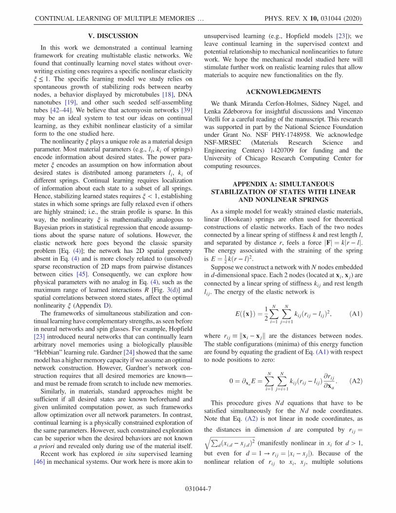
The crucial property of this family of spring potentials isthe force behavior at large strains, far beyond the coreu ≫ 1. At large strains the force applied by the springs isF ∼ uξ−1, a form which goes through an important tran-sition at ξ ¼ 1. For springs with ξ > 1, the restoring forcegrows with strain, while for ξ < 1 the force diminishes.This transition causes an important change of behaviorwhen such spring potentials are summed together, as shownin Fig. 9. The minima of individual springs are preservedfor ξ < 1, while these minima are overwritten for springswith ξ > 1. We conclude that only springs with ξ < 1 (ormore generally, springs whose force diminishes with range)enable continual learning. In continual learning, we wouldlike the information about each stored state to be localizedto a subset of springs, and that adding more springs for newstates does not overwrite the previously stored information.Figure 9 clarifies that springs whose force grows with strainare unfit for this purpose.

APPENDIX C: NUMERICAL EXPLORATION OFMECHANICAL NETWORKS

Testing predictions about learning elastic networksrequires the numerical construction of such networksand the ability to explore their potential energy landscape.This Appendix describes some of the technical aspects

involved in simulating these networks and deducing theirproperties. The codes to produce and study the elasticnetworks are implemented in PYTHON and available uponrequest.

1. Network construction

The elastic networks simulated for this work consist ofNnodes embedded in a 2D box of size 1 × 1. For each desiredsystem configuration (stored state), node positions aresampled uniformly at random within the boundary of thebox. Each multistable system of this type with M states isthus described by M × N × 2 positions in the range [0, 1].Springs are attached between pairs of nodes according tothe paradigm studied (simultaneous stabilization, continuallearning).For the simultaneous stabilization model, we fully

connect all pairs of nodes in the system with linear springs(ξ ¼ 2). These springs are chosen to take into account all ofthe desired states simultaneously. The choice of springs(stiffness and rest length values) is made by solving the setof equations (A2) in Appendix A. Construction of fullyconnected, simultaneously stabilized networks with non-linear springs (ξ ≠ 2) is facilitated by optimizing forces atthe desired stored states (Appendix A).Systems with learned states are constructed by attaching

a set of springs between pairs of nodes for each stored state.We generally do not fully connect the nodes, instead optingto connect a spring between nodes within a certain chosendistance R. All springs in this paradigm have the samespring stiffness k, core size σ, and nonlinearity parameter ξ.The springs only differ in their rest length, chosen so thatthe springs are relaxed in their respective state. Thus,learning is “easy” in the sense that no computation isrequired to choose the new set of springs in new storedstates. This suggests learning can be performed by a rathersimple, physically passive system, whose time evolutiondepends only on its current configuration.

2. Estimation of attractor size and barrier height

When M > 1 states are encoded into a network, it is ofimmediate interest to check whether these states are stableat all. We define a stable state X⃗ðmÞ (N × 2 spatial vector) bythe following requirement: when the system is releasedfrom X⃗ðmÞ and allowed to relax to a nearby stable minimumof the potential energy landscape, the relaxed configurationX⃗ðmÞ� is close in configuration space to X⃗ðmÞ. We consider

states to be preserved if the average displacement perdegree of freedom after relaxation is much smaller than thesize of the box. The potential core size σ is used as thisstability cutoff ½ðkX⃗ðmÞ

� − X⃗ðmÞkÞ=2N� < σ, where the typ-ical core size is ∼1% of the box size. If the differentencoded states pass this test, we say that the states arestable, and the encoding was successful. See Appendix Dfor more details on the stability of stored states.

FIG. 9. The sum energy of two springs goes through a transitionat ξ ¼ 1. The energy minimum of each spring is preserved forξ < 1, while these minima are overwritten for ξ > 1. In essence,the information on minima of ξ < 1 springs is stored with eachindividual spring. (Black dotted lines correspond to the individualpotentials of two nonlinear springs with given ξ, bold blue linesshow the sum of the two potentials, shifted up for clarity).

CONTINUAL LEARNING OF MULTIPLE MEMORIES … PHYS. REV. X 10, 031044 (2020)

031044-9

In an effort to find optimal schemes for storing stablestates in elastic networks, basic stability does not suffice,and we require additional measures of merit. A naturalapproach is to study the attractor basins of the encodedstates, specifically their spatial extent and the energeticbarriers surrounding them. The larger the attractor basin,the configuration can more reliably be retrieved when thesystem is released farther away from its minimum. Highenergy barriers surrounding the state basins improve theirstability when the system is subjected to finite temperaturesor other types of noise.Unfortunately both attractor size and energy barrier are

nonlocal properties of the attractor, requiring many high-dimensional measurements away from the stable state.Rather than exhaustively studying the attractor basin shapeand height, we employ a procedure as follows. At the stablestate, choose a random direction and take the system asmall amount in that direction. Relax the system from thenew position and verify whether it relaxed into the samestable state. If so, repeat the last step, but take the systemslightly farther away in the same direction as before. Repeatthese steps until the system no longer relaxes to the initialstate, but instead reaches another stable point of thelandscape. Measuring the distance required to move thesystem in order to escape the attractor, and the energy atthat distance, furnishes an estimate of both the attractor sizeand the energy barriers around it. We repeat the aboveprocess to average the results over many different randomdirections in configuration space.An important correction is needed for the above esti-

mation, in particular for the flatter spring potentials ξ ≪ 1.Attractors arising from these potentials tend to be very flatfar from the core region σ surrounding each stored state.Although flat regions mathematically belong to someattractor basin, releasing the system in these regions willrequire long relaxation times, and relaxation dynamics arehighly unstable to external noise. We therefore define a“useful” attractor, such that the gradient that leads relax-ation toward the stable point is large enough. In practice,we cut off the attractor defined by the previous algorithmwhen the relaxation force is smaller than a fraction (∼0.5)of the typical force within the core distance σ. The inclusionof this force (gradient) requirement gives rise to an optimalnonlinearity value 0 < ξ < 1 for learned states.

APPENDIX D: STABILITY OF LEARNEDSTATES

We established the necessity of nonlinear springs as ameans of continually learning multiple stable states in anelastic network. In this Appendix, we discuss somelimitations of this idea, such as the finite capacity ofnode-spring networks, and the effect of connectivity withina state and correlations between states on the quality oflearning.

1. Storing capacity

Nonlinear spring networks (with ξ < 1) can stabilizemultiple states through sparsity—springs associated with acertain state dominate the response of the network when itis situated close to that state. Springs associated with otherstates are highly stretched, yet apply small forces thatfurther diminish at high strains. Still, force contributions ofsprings unrelated to the desired state are finite and act todestabilize that state.The learned networks studied in this work exhibit

destabilization of learned states due to the effect of springsassociated with other stored states. Figure 10(a) shows atypical scenario observed in these networks, where adesired state is stable when the overall number of learnedstates is low. Then, an abrupt threshold (capacity) is passedafter which the state destabilizes completely and the systemrelaxes into a configuration that looks completely differentfrom the desired stored state. Generically, all learned statesfail in this way at a similar capacity value [Fig. 10(b)]. Thiscapacity is well defined and observed to depend on theparameters of the system, such as size N and nonlinearity ξ.Let us now argue for a scaling relation of the storing

capacity. Suppose a system of N nodes is used to learnM þ 1 states. In configurations close to state 1, N springswill apply a stabilizing force FS, while the rest N ×Msprings will act to destabilize the state with force FDS. Allstabilizing springs provide a force in the same stabilizingdirection such that F ∼ N. If we assume the N ×Mdestabilizing forces due to unrelated springs are randomlyoriented and similar in magnitude, the total destabilizingforce would behave like a random walk and have amagnitude FDS ∼

ffiffiffiffiffiffiffiffiffiffiffiffiffiffiN ×M

p. The capacity of the system

is reached when the magnitude of the destabilizing force isequal to that of the stabilizing force, so that

FDSðMCÞ ∼ FS → MC ∼ N: ðD1ÞThe capacity of a learning network is expected to scale

linearly with system size, similarly to other Hopfield-inspired learning models [23]. This prediction was testedin networks of sizes N ¼ 6–26 and for several values of thenonlinearity ξ. Results shown in Fig. 10(c) are consistentwith the linear scaling suggested above. Theoretical argu-ments of a similar nature suggest another scaling relationMC ∼ expð−ξÞ, also in agreement with numerical data.However, we regard the capacity dependence on non-linearity to be of lesser interest, as other metrics for qualityof encoding (barrier height and attractor size) are moreimportant for the robustness of learning.

2. Connectivity of nodes

It is well known that the rigidity of elastic networksstrongly depends on node coordination—the number ofsprings connected to the different nodes. Rigid networksare characterized by coordination numbers exceeding the

STERN, PINSON, and MURUGAN PHYS. REV. X 10, 031044 (2020)

031044-10

Maxwell condition [47]. A stable state of the overcon-strained network can be understood as a minimum point ofthe energy landscape constructed of the spring potentials.Further increasing the coordination of nodes—or theirconnectivity to other nodes—results in stable states sur-rounded by higher energy barriers.This argument suggests an intriguing possibility, that

increasing connectivity in a learned network may improvethe stability and quality of the state storage. Such anoutcome is possible as the act of adding more nonlinear(ξ < 1) springs associated with a certain stored state is notexpected to significantly alter the state itself, since the restlengths are chosen to stabilize this state. On the other hand,the extra springs may increase the height of energy barrierssurrounding the state, making it more stable againsttemperature and noise. Furthermore, increasing connectiv-ity may also enlarge the attractor regions of stored states, asthe extra constraints induced by the new springs maysuppress “distractor” states (spurious energy minima due topartial satisfaction of the frustrated interactions).In the context of our learning paradigm, connectivity is

controlled by the effective radius of rod growth R. If statesare constructed by randomly placing N nodes in a d-dimensional square box of length L, it is easy to see that theaverage connectivity scales as hZi ∼ NRd while R ≪ L.We use N ¼ 100, ξ < 1 networks to test the effect of nodeconnectivity on the attractor size of stored states. Resultspresented in Figs. 11(a)–11(c) verify that the quality ofstate storage, as measured by the attractor size of states,improves with their connectivity.

3. State similarity

In most of this work we considered stored states thatare completely uncorrelated between themselves; i.e., the

position of a node in each stored state is independent of itsposition in other states. In practice, it might be easier toconceive of elastic networks whose different stable statesare not too different from one another, in which neighbor-ing nodes in one configuration will remain neighbors inother configurations. Furthermore, some applications (e.g.,classification of similar objects) may require differentstored states to be correlated to differing extents. In general,encoding correlated (i.e., similar) states is expected tonegatively affect the stability of these states and theirquality (as measured by attractor properties as size andbarrier heights).To test the impact of similarity between states, we

embedded a N ¼ 100 network with states in which theaverage displacement of nodes in successive states wascontrolled. Figures 11(d)–11(f) show that the larger thedifference between states, the larger their respective attrac-tor sizes. In addition, larger differences between statesallows their stabilization at higher ξ values, which isexpected to improve the heights of energy barriers sur-rounding them and further suppress distractor states. Still,we show that it is possible to encode multiple states inelastic networks, even when the average difference betweenstored states is a small multiple of σ (the potential core size,within which states are indistinguishable).

APPENDIX E: CONTINUAL LEARNINGREQUIRES NONLINEAR, UNSTRAINED

SPRINGS

In the main text we laid out arguments for the necessityof nonlinear ξ < 1 springs for continual learning. Here, weexpand on these considerations, specifically showingthat continual learning always results in deformation oflearned states. Thus, nonlinear ξ < 1 springs, causing such

(a) (b) (c)

FIG. 10. Programming stored states using the learning paradigm exhibits finite capacity. (a) Each stored state is affected by springsassociated with other states. Initially the new springs have a small effect and the state remains a stable attractor. However, eventuallystates destabilize due to the forces exerted by the other stored states (blue squares denote a certain stored state, black circles show thenearby stable configuration). This state fails when 13 states are simultaneously encoded (N ¼ 100, ξ ¼ 0.6, σ ¼ 10−2L). (b) When nodedisplacement is averaged over stored states, we observe a sharp failure of all states at a specific load, defined as the capacity (12–13states in this case). (c) Capacity scales linearly with system size N.

CONTINUAL LEARNING OF MULTIPLE MEMORIES … PHYS. REV. X 10, 031044 (2020)

031044-11

deformations to be small, are essential for continual learning.We also discuss why the nonlinear springs need to beunstrained in their respective states to stabilize them.

1. Continual learning always deforms learned states

Suppose we have M sets of linear ξ ¼ 2 springs, chosensuch that a state xð1Þ is stable. These spring sets are definedso that one such set can be modified to accommodate asingle new stable state in the system. In this setting, we canwrite a force balance equation similar to Eq. (A2):

0¼ ∂xaEðxð1ÞÞ

¼XMm¼1

XNi¼1

XNj¼iþ1

kmijðrmijðxð1ÞÞ− lmijÞ∂rmijðxð1ÞÞ

∂xa: ðE1Þ

Continually learning a new state xð2Þ is only allowedthrough the modification of the springs of set no. 2.

Suppose we devise a learning rule that after a shortapplication, infinitesimally changes the properties of springset no. 2:

k2ij → k2ij þ Δk2ij;

l2ij → l2ij þ Δl2ij:

Reevaluating the force equation, we note that state xð1Þremains stable only if the force balance is maintained giventhis spring modification:

0 ¼ ∂xaEðxð1Þ; k2 þ Δk2; l2 þ Δl2Þ − ∂xaEðxð1Þ; k2; l2Þ:

Maintaining first-order contributions in Δk2, Δl2, weobtain

(a) (b) (c)

(d) (e) (f)

FIG. 11. Effects of node connectivity and state similarity on the quality of encoding the stored states. (a)–(c) Connectivity betweennodes hZi increases with the effective connection radius R. We find that the more internally connected a state is, the larger its attractorsize, and higher the optimal value of the nonlinearity parameter ξ (N ¼ 100, σ ¼ 5 × 10−3L). (d)–(f) Trying to store similar states ismore difficult than random states. When the mean distance between nodes in successive states is small, attractor’s basin is also small, andsuccessful encoding requires small values of ξ and flat potentials (N ¼ 100, σ ¼ 5 × 10−3L). Results averaged over six simulations ofrandom continual learning networks.

STERN, PINSON, and MURUGAN PHYS. REV. X 10, 031044 (2020)

031044-12

0 ¼XNi¼1

XNj¼iþ1

�Δk2ijk2ij

−Δl2ij

r2ijðxð1ÞÞ − l2ij

�

× ðr2ijðxð1ÞÞ − lmijÞ∂r2ijðxð1ÞÞ

∂xa: ðE2Þ

This is a set of linear equations in Δk2, Δl2. The numberof variables is the number of spring parameters, which inoverconstrained networks is larger than the number ofequations (locations of the nodes). Finding solutions tothese equations is possible only if information of state xð1Þis available. This condition prohibits any generic locallearning rule that does not have information about previousstates. In other words, a generic change to the parameters ofthe springs of set no. 2, ignorant of state no. 1, will give riseto finite residual forces in state no. 1, deforming it from theoriginal state.While we cannot generically solve the force balance

equations for networks of ξ ≠ 2 springs, the above argu-ments still hold: a generic change of the spring parameter ofany set (ignorant of previous encoded states) will deformthe encoded states [e.g., as in Fig. 10(a)].

2. Nonlinear, ξ < 1 springs support continual learning

Suppose a state xð1Þ is encoded by a single unstrainedspring with nonlinearity ξ and core size σ. Now, we applyan external force on the spring Ferase to extend it by somelength δx, as shown in Fig. 4(a). The extension can becomputed by considering the force balance on the spring(u ¼ δx=σ):

Fspring ¼ kσξ−1u1þ 1

2ξu2

ð1þ u2Þ2−ð1=2Þξ ¼ Ferase:

If the deformation is large (u ≫ 1), this expressionsimplifies to

Ferase ≈1

2kξσξ−1uξ−1 ¼ 1

2kξδxξ−1;

δx ≈�2Ferase

kξ

�1=ξ−1

: ðE3Þ

Instead, if the deformation is small (u ≪ 1), we mayperform a Taylor expansion of the spring force aroundu ¼ 0 to find

δxσ≈Ferase

kσ1−ξ: ðE4Þ

If we assume that the erasure force Ferase is caused by asecond spring with the same parameters ξ, σ, but which ishighly strained δxð2Þ ≡ R ≫ σ, we can use Eq. (E3) to seethat Ferase ≈ 0.5kξRξ−1. Putting this force back in Eq. (E4),we finally obtain

δxσ≈ξ

2

�Rσ

�1−ξ

: ðE5Þ

Since we assume R ≫ σ, we see that for ξ < 1, thedeformation δx=σ → 0, which is consistent with our initialassumption. On the other hand, for ξ > 1, the deformationdiverges and our approximation fails. Fortunately, we mayinstead plug the erasure force in Eq. (E3), to find that forξ > 1 springs, the extension is δx ≈ R ≫ σ (as observed inFig. 9). There is thus a transition in the spring extension dueto the erasure force of another spring, at ξ ¼ 1. Nonlinearsprings with ξ < 1 will show a very small deformationδx ≪ σ, while springs with ξ > 1 will exhibit δx ≫ σ.For finite values of the core size σ, the aforementioned

considerations are valid for small enough erasure forces. Ifthe erasure force is large, Eq. (E4) becomes inconsistentwith the assumption that δx=σ ≪ 1, and the argument fails.For ξ < 1 springs, this happens if the erasure forcesurpasses a threshold, Ferase > FT , the largest restoringforce afforded by the spring. The threshold force can befound by computing the second derivative of the springenergy and equating to zero:

d2Edu2

∼ð1þ 3

2ξu2Þð1þ u2Þ þ ðξ − 4Þu2ð1þ 1

2ξu2Þ

ð1þ u2Þ3−0.5ξ ¼ 0:

This equation can be solved as a function of the non-linearity ξ to find a deformation that maximizes therestoring force:

u� ¼ δx�

σ¼

ffiffiffiffiffiffiffiffiffiffiffiffiffiffiffiffiffiffiffiffiffiffiffiffiffiffiffiffiffiffiffiffiffiffiffiffiffiffiffiffiffiffiffiffiffiffiffiffiffiffiffiffiffiffiffiffiffiffiffiffiffiffiffiffiffiffiffiffiffiffiffiffiffiffiffiffiffiffiffiffiffiffiffiffiffiffiffi17ξ2 − 52ξþ 36

p− 5ξþ 6

2ðξ2 − ξÞ

s∼ oð1Þ:

Note that this result does not depend on σ, so that themaximum restoring force, or threshold force, is

FT ∼ kσξ−1: ðE6Þ

Thus, for unstrained nonlinear springs with ξ < 1 andsmall cores σ → 0, the external force required fordeforming an encoded state is large. Such encoded statesare expected to be robust to the interference of other statesand sources of noise (e.g., temperature).

3. Continual learning fails in prestrained networks

Our learning rule involves addition of unstrained non-linear springs in every new (geometric) state to be encodedin the network. Here we show that using prestrained springscannot facilitate continual learning. Essentially, we arguethat applying external forces on prestrained springs alwaysdestabilizes the state.Consider a spring with stiffness k and rest length l.

Suppose the spring is strained to an extent r ≠ l in a stable(desired) state of the network. We say this spring is

CONTINUAL LEARNING OF MULTIPLE MEMORIES … PHYS. REV. X 10, 031044 (2020)

031044-13

prestrained, with strain s ¼ r − l. The magnitude of theforce exerted by the spring (given nonlinearity parameter ξand σ ≪ r − l) in that stable state is F ¼ kjsjξ−1. Now, weapply some constant external force Ferase parallel to the axisof the spring. The new equilibrium position of the springwill be such that F þ Ferase ¼ 0, so that the new strain iss� ∼ ðFeraseÞ1=ðξ−1Þ. For 1 < ξ < 2 springs, the state willdeform at least in proportion to

ffiffiffiffiffiffiffiffiffiffiffiFerase

p. For the strongly

nonlinear springs ξ < 1, the result is in fact much worse,and s� tends to �∞ for any magnitude of Ferase. Thus, forξ < 1 springs, we conclude that the original prestrainedstate was an unstable equilibrium. Continual learningnetworks, which by definition must be stable to “external”forces due to competing states, can only be realized byusing unstrained springs with s ≪ σ to encode stable states.

[1] U. Feudel, Complex Dynamics in Multistable Systems, Int. J.Bifurcation Chaos Appl. Sci. Eng. 18, 1607 (2008).

[2] J. L. Silverberg, J.-H. Na, A. A. Evans, B. Liu, T. C. Hull,C. D. Santangelo, R. J. Lang, R. C. Hayward, and I. Cohen,Origami Structures with a Critical Transition to BistabilityArising from Hidden Degrees of Freedom, Nat. Mater. 14,389 (2015).

[3] S. Waitukaitis, R. Menaut, B. G.-G. Chen, and M.van Hecke, Origami Multistability: From Single Verticesto Metasheets, Phys. Rev. Lett. 114, 055503 (2015).

[4] J. T. B. Overvelde, T. A. De Jong, Y. Shevchenko, S. A.Becerra, G. M. Whitesides, J. C. Weaver, C. Hoberman,and K. Bertoldi, A Three-Dimensional Actuated Origami-Inspired Transformable Metamaterial with MultipleDegrees of Freedom, Nat. Commun. 7, 10929 (2016).

[5] S. Shan, S. H. Kang, J. R. Raney, P. Wang, L. Fang, F.Candido, J. A. Lewis, and K. Bertoldi, Multistable Archi-tected Materials for Trapping Elastic Strain Energy, Adv.Mater. 27, 4296 (2015).

[6] K. Bertoldi, V. Vitelli, J. Christensen, and M. van Hecke,Flexible Mechanical Metamaterials, Nat. Rev. Mater. 2,17066 (2017).

[7] G. Steinbach, D. Nissen, M. Albrecht, E. V. Novak, P. A.Sánchez, S. S. Kantorovich, S. Gemming, and A. Erbe,Bistable Self-Assembly in Homogeneous Colloidal Systemsfor Flexible Modular Architectures, Soft Matter 12, 2737(2016).

[8] L. Wu, X. Xi, B. Li, and J. Zhou, Multi-Stable MechanicalStructural Materials, Adv. Eng. Mater. 20, 1700599 (2018).

[9] Y. Yang, M. A. Dias, and D. P. Holmes, MultistableKirigami for Tunable Architected Materials, Phys. Rev.Mater. 2, 110601 (2018).

[10] K. Che, C. Yuan, J. Wu, H. J. Qi, and J. Meaud, Three-Dimensional-Printed Multistable Mechanical Metamateri-als with a Deterministic Deformation Sequence, J. Appl.Mech. 84, 011004 (2017).

[11] H. Yang and L. Ma,Multi-Stable Mechanical Metamaterialswith Shape-Reconfiguration and Zero Poisson’s Ratio,Mater. Des. 152, 181 (2018).

[12] H. Fu et al., Morphable 3D Mesostructures and Micro-electronic Devices by Multistable Buckling Mechanics,Nat. Mater. 17, 268 (2018).

[13] J. Z. Kim, Z. Lu, S. H. Strogatz, and D. S. Bassett,Conformational Control of Mechanical Networks, Nat.Phys. 15, 714 (2019).

[14] H. Sayama, I. Pestov, J. Schmidt, B. J. Bush, C. Wong, J.Yamanoi, and T. Gross, Modeling Complex Systems withAdaptive Networks, Comput. Math. Appl. 65, 1645 (2013).

[15] D. Hu andD. Cai, Adaptation andOptimization of BiologicalTransport Networks, Phys. Rev. Lett. 111, 138701 (2013).

[16] J. Gräwer, C. D. Modes, M. O. Magnasco, and E. Katifori,Structural Self-Assembly and Avalanchelike Dynamics inLocally Adaptive Networks, Phys. Rev. E 92, 012801 (2015).

[17] S. L. Gupton and C.M. Waterman-Storer, SpatiotemporalFeedback between Actomyosin and Focal-Adhesion SystemsOptimizes Rapid Cell Migration, Cell 125, 1361 (2006).

[18] H. Hess and J. L. Ross, Non-Equilibrium Assembly ofMicrotubules: From Molecules to Autonomous ChemicalRobots, Chem. Soc. Rev. 46, 5570 (2017).

[19] A. M. Mohammed and R. Schulman, Directing Self-Assembly of DNA Nanotubes Using Programmable Seeds,Nano Lett. 13, 4006 (2013).

[20] A. M. Mohammed, P. Šulc, J. Zenk, and R. Schulman, Self-Assembling DNA Nanotubes to Connect MolecularLandmarks, Nat. Nanotechnol. 12, 312 (2017).

[21] M. Rumpler, A. Woesz, J. W. C. Dunlop, J. T. van Dongen,and P. Fratzl, The Effect of Geometry on Three-DimensionalTissue Growth, J. R. Soc. Interface 5, 1173 (2008).

[22] A. Tero, R. Kobayashi, and T. Nakagaki, PhysarumSolver: A Biologically Inspired Method of Road-NetworkNavigation, Physica (Amsterdam) 363A, 115 (2006).

[23] J. J. Hopfield, Neural Networks and Physical Systems withEmergent Collective Computational Abilities, Proc. Natl.Acad. Sci. U.S.A. 79, 2554 (1982).

[24] E. Gardner, The Space of Interactions in Neural NetworkModels, J. Phys. A 21, 257 (1988).

[25] J. Kirkpatrick, R. Pascanu, N. Rabinowitz, J. Veness, G.Desjardins, A. A. Rusu, K. Milan, J. Quan, T. Ramalho, A.Grabska-Barwinska, D. Hassabis, C. Clopath, D. Kumaran,and R. Hadsell, Overcoming Catastrophic Forgetting inNeural Networks, Proc. Natl. Acad. Sci. U.S.A. 114, 3521(2017).

[26] J. W. Rocks, H. Ronellenfitsch, A. J. Liu, S. R. Nagel, andE. Katifori, Limits of Multifunctionality in TunableNetworks, Proc. Natl. Acad. Sci. U.S.A. 116, 2506 (2019).

[27] D. Hexner, A. J. Liu, and S. R. Nagel, Role of LocalResponse in Manipulating the Elastic Properties ofDisordered Solids by Bond Removal, Soft Matter 14, 312(2018).

[28] M. Isobe and K. Okumura, Initial Rigid Response andSoftening Transition of Highly Stretchable Kirigami SheetMaterials, Sci. Rep. 6, 24758 (2016).

[29] J. Ma, J. Song, and Y. Chen, An Origami-Inspired Structurewith Graded Stiffness, Int. J. Mech. Sci. 136, 134 (2018).

[30] M. Dogterom and T. Surrey, Microtubule OrganizationIn Vitro, Curr. Opin. Cell Biol. 25, 23 (2013).

[31] J. Hertz, A. Krogh, and R. G. Palmer, Introduction to theTheory of Neural Computation (Addison-Wesley/Addison-Wesley Longman, Reading, MA, 1991).

STERN, PINSON, and MURUGAN PHYS. REV. X 10, 031044 (2020)

031044-14

[32] D. J. Amit, H. Gutfreund, and H. Sompolinsky, StoringInfinite Numbers of Patterns in a Spin-Glass Model ofNeural Networks, Phys. Rev. Lett. 55, 1530 (1985).

[33] D. J. Amit, H. Gutfreund, and H. Sompolinsky, Spin-GlassModels of Neural Networks, Phys. Rev. A 32, 1007 (1985).

[34] R. Tibshirani, Regression Shrinkage, and Selection via theLasso, J. R. Stat. Soc., Ser. B 58, 267 (1996).

[35] H. Zou and T. Hastie, Regularization and Variable Selectionvia the Elastic Net, J. R. Stat. Soc., Ser. B 67, 301 (2005).

[36] T. Hastie, R. Tibshirani, and M. Wainwright, StatisticalLearning with Sparsity: The Lasso and Generalizations(CRC Press, Boca Raton, FL, 2015).

[37] Y. LeCun, C. Cortes, and C. J. Burges, MNIST HandwrittenDigit Database, http://yann.lecun.com/exdb/mnist.

[38] N. Pashine, D. Hexner, A. J. Liu, and S. R. Nagel, DirectedAging, Memory, and Natures Greed, Sci. Adv. 5, eaax4215(2019).

[39] O. Chaudhuri, S. H. Parekh, and D. A. Fletcher, ReversibleStress Softening of Actin Networks, Nature (London) 445,295 (2007).

[40] F. J. Lockett, Nonlinear Viscoelastic Solids (AcademicPress, London, 1972).

[41] J. D. Humphries, P. Wang, C. Streuli, B. Geiger, M. J.Humphries, and C. Ballestrem, Vinculin Controls Focal

Adhesion Formation by Direct Interactions with Talin andActin, J. Cell Biol. 179, 1043 (2007).

[42] S. Li, P. He, J. Dong, Z. Guo, and L. Dai, DNA-DirectedSelf-Assembling of Carbon Nanotubes, J. Am. Chem. Soc.127, 14 (2005).

[43] J. D. Hartgerink, J. R. Granja, R. A. Milligan, and M. R.Ghadiri, Self-Assembling Peptide Nanotubes, J. Am. Chem.Soc. 118, 43 (1996).

[44] W. J. Blau and A. J. Fleming, Materials Science. DesignerNanotubes by Molecular Self-Assembly, Science 304, 1457(2004).

[45] A. Javanmard and A. Montanari, Localization fromIncomplete Noisy Distance Measurements, Found. Comput.Math. 13, 297 (2013).

[46] M. Stern, C. Arinze, L. Perez, S. E. Palmer, and A.Murugan, Supervised Learning through Physical Changesin a Mechanical System, Proc. Natl. Acad. Sci. U.S.A. 117,14843 (2020).

[47] J. C. Maxwell, L. On the Calculation of the Equilibrium andStiffness of Frames, London, Edinburgh, Dublin Philos.Mag. J. Sci. 27, 294 (1864).

[48] J. D. Paulsen and N. C. Keim, Minimal descriptionsof cyclic memories, Proc. R. Soc. A 475, 20180874(2019).

CONTINUAL LEARNING OF MULTIPLE MEMORIES … PHYS. REV. X 10, 031044 (2020)

031044-15