Continuation and bifurcation analysis of delay …kouzn101/rosz.pdfContinuation and bifurcation...

Continuation and bifurcation analysis of delaydifferential equations

Dirk Roose1 and Robert Szalai2

1 Department of Computer Science, Katholieke Universiteit Leuven, Belgium2 Department of Engineering Mathematics, University of Bristol, United Kingdom

Mathematical modeling with delay differential equations (DDEs) is widelyused in various application areas of science and engineering (e.g., in semi-conductor lasers with delayed feedback, high-speed machining, communicationnetworks, and control systems) and in the life sciences (e.g., in population dy-namics, epidemiology, immunology, and physiology). Delay equations have aninfinite-dimensional state space because their solution is unique only when aninitial function is specified on a time interval of length equal to the largestdelay. Consequently, analytical calculations are more difficult than for ordin-ary differential equations andnumerical methods are generally the only wayto achieve a complete analysis, prediction and control of systems with timedelays.

Delay differential equations are a special type of functional differentialequation (FDE). In FDEs the time evolution of the state variable can dependon the past in an arbitrary way as long as the dependence is a boundedfunction of the past. However, DDEs impose a constraint on this dependence,namely that the evolution depends only on certain past values of the state atdiscrete times. (We do not consider here the case of distributed delay.) Thedelays can be constant or state dependent. The equations can also involvedelayed values of the derivative of the state, which leads to equations of neutraltype.

In this chapter we mainly discuss the simplest case, namely a finite numberof constant delays. Specifically, we consider a nonlinear system of DDEs withconstant delays τj > 0, j = 1, . . . ,m, of the form

x′(t) = f(x(t), x(t− τ1), x(t− τ2), . . . , x(t− τm), η), (1)

where x(t) ∈ Rn, and f : R(m+1)n+p → Rn is a nonlinear smooth functiondepending on a number of (time-independent) parameters η ∈ Rp. We assumethat the delays are in increasing order and denote the maximal delay by

τ = τm = maxi=1,...,m

τi.

2 Dirk Roose and Robert Szalai

A solution segment is denoted by xt = xt(θ) = x(t + θ) ∈ C, θ ∈ [−τ, 0].Here C = C([−τ, 0];Rn) is the space of continuous functions mapping thedelay interval into Rn. For a fixed value of the parameter η, a solution x(t)of (1) on t ∈ [0,∞) is uniquely defined by specifying a function segment x0

as an initial condition. A discontinuity in the first derivative of x(t) generallyappears at t = 0 and is propagated in time, even if f and φ are infinitelysmooth. However, the solution operator of (1) smooths the solution, meaningthat discontinuities appear in higher and higher derivatives as time increases.

A DDE can be approximated by a system of ordinary differential equations(ODEs) and so standard numerical methods for ODEs could be used. However,to obtain an accurate approximation a high-dimensional system of ODEs isneeded, and this leads to expensive numerical procedures. During the last dec-ade, more efficient and more reliable numerical methods have been developedspecifically for DDEs. In this chapter we survey those numerical methods forthe continuation and bifurcation analysis of DDEs that are implemented inthe software packages DDE-Biftool [25, 26] and PDDE-Cont [73]. Whereappropriate, we also briefly describe alternative numerical methods. Note thatwe do not discuss time integration of DDEs; for this topic see, e.g., [2] and[6].

The structure of this chapter is as follows. In Sec. 1 we discuss numer-ical methods to compute the right-most characteristic roots of steady-statesolutions. In Sec. 2 we describe collocation methods for computing periodicsolutions and their dominant Floquet multipliers. Section 3 presents defin-ing systems for codimension-one bifurcations of periodic solutions that allowone to compute the location of bifurcation points accurately. Computationof connecting orbits is discussed in Sec. 4 and of quasiperiodic solutions isdiscussed in Sec. 5. In Sec. 6 we briefly discuss how to deal with specialtypes of DDEs, specifically, equations of neutral type and DDEs with state-dependent delays. In Sec. 7 we discuss specific details of the software packagesDDE-Biftool and PDDE-Cont. Their functionality is illustrated in Sec. 8,where we present the bifurcation analysis of several DDE models of practicalrelevance. Finally, conclusions and an outlook can be found in Sec. 9.

1 Stability of steady-state solutions

In this and the next section we assume that the parameter η is fixed and weomit it from the equations. A steady-state solution x(t) ≡ x? of (1) satisfiesthe nonlinear system

f(x?, x?, x?, . . . , x?) = 0. (2)

The (local) stability of x? is determined by the stability of (the zero solu-tion of) the linearized equation

y′(t) = A0y(t) +∑mj=1Ajy(t− τj), (3)

Continuation and bifurcation analysis of delay differential equations 3

where Aj ∈ Rn×n denotes the partial derivative of f with respect to its(j+1)-th argument, evaluated at the steady-state solution x?. The linearizedequation (3) is asymptotically stable if all its roots λ of the characteristicequation

det(λI −A0 −m∑

j=1

Aje−λτj ) = 0 (4)

lie in the open left half-plane (i.e., Re(e(λ)) < 0); see, e.g., [38, 58, 70]. Equa-tion (4) has an infinite number of roots λ, known as the characteristic roots.However, the number of characteristic roots with real part larger than a giventhreshold is finite. Hence, to analyse the stability of a steady-state solution,one must determine reliably all roots satisfying Re(e(λ)) > r, for a given r < 0close to zero.

Analytical conditions for stability can be found in Stepan [70] and Hassard[42]. These conditions are deduced by using the argument principle of complexanalysis, and they give a practical method for determining stability. In recentyears, numerical methods have been developed to compute approximations tothe right-most (stability-determining) characteristic roots of (4), by using adiscretization either of the solution operator of (3) or of the infinitesimal gen-erator of the semi-group of the solution operator of (3). The solution operatorS(t) of the linearized equation (3) maps an initial function segment onto thesolution segment at time t, i.e.,

S(t)y(·)(θ) = y(t+ θ), − τ ≤ θ ≤ 0, t ≥ 0. (5)

This operator has eigenvalues µ, which are related to the characteristic rootsvia the equation µ = eλt [63]. To determine the stability, we are interestedin the dominant eigenvalues that, if t is large, are well separated. This canbe an advantage for the eigenvalue computation, but the time integrationitself may be costly. In Sec. 1.1 we describe a reliable way to compute thedominant eigenvalues of S(h) where h is the time step of a linear multistep(LMS) method.

Since S(t) is a strongly continuous semi-group [36, 38], one can define thecorresponding infinitesimal generator A by

Ay = limt→0+

S(t)y − y

t. (6)

For (3) the infinitesimal generator becomes

Ay(θ) = y′(θ), y ∈ D(A)D(A) = y ∈ C : y′ ∈ C and y′(0) =

∑mj=0Ajy(−τj).

(7)

Both operators can be discretised by spectral discretizations or time in-tegration methods; this always leads to a representation by some matrix.Eigenvalues of this matrix yields approximations to the right-most character-istic roots. Hence, for computational efficiency it is important that the size of


the resulting matrix eigenvalue problem is small, or at least that the stabilitydetermining eigenvalues can be computed efficiently. iterative method, suchas subspace iteration. Accurate characteristic roots can be found by usingNewton iterations on the characteristic equation

(λI −A0 −∑mj=1Aje

−λτj )v = 0,v0T v = 1

(8)

where v ∈ Rn and v0 ∈ Rn, to obtain accurate characteristic roots λ (and thecorresponding eigenfunctions veλt). The difference between the approximateand the corrected roots gives an indication of the accuracy of the approxim-ations.

Below we describe how the characteristic roots can be computed via an ap-proximation of the solution operator by time integration, which is the methodthat is implemented in DDE-Biftool. We also briefly comment on other ap-proaches.

1.1 Approximation of the solution operator by a time integrator

A natural way to approximate the solution operator is to write the numericaltime integration of the linearized equation as a matrix equation. Engelborghset al. [27] have proposed and analysed the use of a linear multistep methodwith constant steplength h to approximate the solution operator S(h). Thedelay interval [−τ, 0] (slightly extended to the left and the right; see below) isdiscretized by using an equidistant mesh with mesh spacing h, and a solutionis represented by a discrete set of points yi := y(ti) with ti = ih. A k-stepLMS method with steplength h to compute yk can be written as

k∑i=0

αiyi = hk∑i=0

βi

(A0yi +

m∑j=1

Aj y(ti − τj)), (9)

where αi and βi are parameters and where (in case ti − τj does not coincidewith a mesh point) the approximations y(ti − τj) are obtained by polynomialinterpolation with s− and s+ points to the left and the right, respectively.

The discretization of the solution operator is the (linear) map between[yLmin , . . . , yk−1]T and [yLmin+1, . . . , yk]T where Lmin = −s− − dτ/he andwhere the mapping is defined by (9) for yk and by a shift for all variablesother than yk. This map is represented by an N ×N matrix, where

N = n(−Lmin + k) ≈ nτ/h. (10)

Since the time step h is small, the eigenvalues µ of this matrix are not wellseparated (most eigenvalues lie close to the unit circle). They can be computedby e.g. the QR method, with a computational cost of the orderN3 ≈ n3(τ/h)3,and so approximations to the characteristic roots can be derived.


To guarantee the reliability of the stability computation, the steplength hin the LMS method (9) should be chosen such that all characteristic roots λwith Re(e(λ)) > r (r < 0) are approximated accurately. Procedures for such asafe choice of h are described in [27, 79] and implemented in DDE-Biftool.They are based on theoretical properties of

(a) the relation between the stability properties of the solution of the linearizedequation (3) and the stability of the discretized equation (9);

(b) an a-priori estimate of the region in the complex plane that includes allcharacteristic roots λ with Re(e(λ)) > r.

Note that the solution operator can also be discretized by using a Runge-Kutta time integrator [10].

1.2 Other approaches

Breda et al. [11] have developed numerical methods to determine the stabil-ity of solutions based on a discretization of the infinitesimal generator. Bydiscretizing the derivative in (7) with a Runge-Kutta or a LMS method, amatrix approximation of A is obtained. The resulting eigenvalue problem islarge and sparse, as in the case when the solution operator is discretized by atime integration method. Breda et al. [12] also proposed a pseudo-spectral dis-cretization of the infinitesimal generator. In this approach, an eigenfunction ofthe infinitesimal generator veλt, t ∈ [−τ, 0], is approximated by a polynomialP (t) of degree p. Collocation for the eigenvalue problem for the infinitisimalgenerator leads to an equation of the form

P ′(ti) = λP (ti), (11)

where the collocation points ti, i = 1...p are chosen as the shifted and scaledroots of an (orthogonal) polynomial of degree p. These equations are augmen-ted with

A0P (0) +∑mj=1AjP (τj) = λP (0), (12)

which introduces the system-dependent information. The resulting matrix ei-genvalue problem has size n(p+1). The first np rows are the Kronecker productof a dense p× (p+1) matrix and the identity matrix. The last block row con-sists of a linear combination of the matrices Aj , j = 0, ...,m and the identity.The matrix is full but can be of much smaller size than in the previous case,due to the ‘spectral accuracy’ convergence, as is shown in the detailed analysispresented in [12].

A pseudo-spectral discretization of the solution operator is proposed in[81, 10]. Here a polynomial approximation P (t) of an eigenfunction, definedon the interval [−τ, h] has to satisfy p collocation conditions of the form

P (ti + h) = µP (ti),


where µ = eλh. These equations are augmented with a condition obtained fromintegrating the linearized equations over an time interval h. When high accur-acy is required, a pseudo-spectral discretization will lead to a more efficientprocedure than when a time integration discretization is used, but numericalexperiments indicate that for low accuracy requirements both approaches arecompetitive [81].

However, for the pseudo-spectral approaches no strategy is known thatguarantees a priori that all characteristic roots with real part larger than rare computed accurately, as is the case with the discretization of the solutionoperator with a LMS method.

2 Periodic solutions

A periodic solution x?(t) of an autonomous system of the form (1) satisfies

x?(t+ T ) = x?(t), ∀t,where T is the period. An extensive literature exists on the existence, stabilityand parameter dependence of periodic solutions; see, e.g., [38, §XI.1-2]. Theseresults are essentially analytical in nature and the corresponding methodshave different rigorous restrictions and cannot be applied to general nonlinearsystems with several delays.

Because of the dependence on the past, periodicity of x(t) at one momentin time, x(t) = x(t+ T ) for some t, does not imply periodicity for the wholesolution. Instead, a complete function segment of length τ has to be repeated.Consequently, a periodic solution to (1) can be found as the solution of thefollowing two-point boundary value problem (BVP),

x′(t) = f(x(t), x(t− τ1), . . . , x(t− τm), η), t ∈ [0, T ]x0 = xT ,p(x, T ) = 0,

(13)

where x0 and xT are function segments on [−τ, 0] and [−τ+T, T ], respectively,the period T is an unknown parameter. Furthermore, p represents a phasecondition that is needed to remove translational invariance. A well-knownexample is the classical integral phase condition [20]

∫ 1

0

u(0)(s)(u(0)(s)− u(s))ds = 0, (14)

where u(0) is a reference solution; see also Chapter 1.Stable periodic solutions of a DDE can be found by numerical time integra-

tion; the convergence of the integration depends on the stability properties ofthe periodic solution [44]. However, both stable and unstable solutions can becomputed by solving the above boundary value problem by either collocationor by approach. Here we only consider collocation methods.


2.1 Collocation

In collocation a periodic solution is computed by using a discrete represent-ation that satisfies the differential equation at a set of collocation points on[0, T ]. Doedel and Leung [21] have computed periodic solutions of DDEs us-ing collocation based on a truncated Fourier series; see also [13] for a similarapproach. This Fourier approach has the advantage that periodicity is auto-matically fulfilled. However, steep gradients in a solution pose problems andit is not possible to determine the solution stability.

Collocation based on piecewise polynomial representations is used in Auto[17] and Content [50] to compute periodic solutions for systems of ordinarydifferential equations; see also Chapters 1and 2. We now discuss how piecewise-polynomial collocation can be used for DDEs. We first rescale time by a factor1/T such that the period is one in the transformed system

x′(t) = Tf (x(t), x(t− τ1/T ), . . . , x(t− τm/T ), η) , for t ∈ [0, 1],x(θ + 1)− x(θ) = 0, for θ ∈ [−τ/T, 0],p(x, T ) = 0.

(15)

A mesh with L+ 1 mesh points 0 = t0 < t1 < . . . < tL = 1 is specified.This mesh is periodically extended to the left with ` points to obtain a meshon [−τ/T, 1] with `+L intervals. In each interval an approximating polynomialof degree d is described in terms of the function values at the representationpoints (using Lagrange polynomials as basis). These function values are de-termined by requiring that the approximating collocation solution fulfills the(time-scaled) differential equations exactly at the collocation points. In eachinterval, the collocation points are typically chosen as the (scaled and shifted)roots of a d-th degree orthogonal polynomial.

The approximating polynomial of degree d on each interval [ti, ti+1], i =−`, . . . , L− 1, can be written as

u(t) =d∑

j=0

u(ti+ jd)Pi,j(t), t ∈ [ti, ti+1], (16)

where Pi,j(t) are the Lagrange polynomials through the representation points

ti+ jd

= ti +j

d(ti+1 − ti), j = 0, . . . , d.

Because polynomials on adjacent intervals share the value at the commonmesh point, this representation is automatically continuous (however, it isnot continuously differentiable at the mesh points).

The approximation u(t) is completely determined by the coefficients

ui+ jd

:= u(ti+ jd), i = −`, . . . , L− 1, j = 0, . . . , d− 1 and uL := u(tL). (17)

We define the starting vector us and the final vector uf , both of length N =n(`d+ 1), as


us := [u−`, . . . , ui+ jd, . . . , u0]T , uf := [uL−`, . . . , ui+ j

d, . . . , uL]T . (18)

The collocation points are obtained as

ci,j = ti + cj(ti+1 − ti), i = 0, . . . , L− 1, j = 1, . . . , d,

from a set of collocation parameters cj , j = 1, . . . , d, e.g., the shifted andscaled roots of the d-th degree Gauss-Legendre polynomial.

A periodic solution for a fixed value of the parameters η is found as thesolution of the following (n((`+L)d+1)+1)×(n(`+L)d+1)+1)-dimensional(nonlinear) system in terms of the unknowns (17) and T ,

u(ci,j) = Tf(u(ci,j), u(ci,j − τ1T ), . . . , u(ci,j − τm

T )), η) = 0,i = 0, . . . , L− 1, j = 1, . . . , d

uf = us,p(u) = 0.

(19)

Here, p again represents a phase condition such as (14).The collocation solution fulfils the time-scaled differential equation exactly

at the collocation points. If ci,j coincides with ti then the right derivative istaken in (19), if it coincides with ti+1 then the left derivative is taken. Takinginto account the periodicity conditions, one can reduce system (19) to thefollowing nonlinear system in the unknowns u = [u0, . . . , uL]T and T ,

u(ci,j) = Tf(u(ci,j), u((ci,j − τ1T )mod 1), . . . , u((ci,j − τm

T ) mod 1), η) = 0,i = 0, . . . , L− 1, j = 1, . . . , d

u0 = uL,p(u) = 0.

(20)Hence, the dimension of the system and the number of unknowns is reducedto (n(Ld+ 1) + 1).

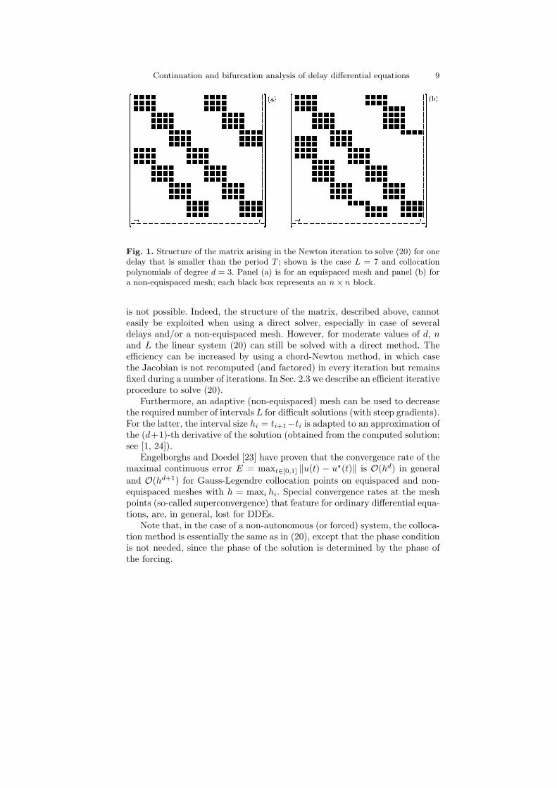
When using Newton’s method to solve (20), the matrix of the linear systemto be solved in each iteration is sparse and has a particular structure, as isshown in Fig. 1. The matrix consists of a (large) nLd×n(Ld+1) matrix filledwith two (circular) bands, bordered by one column and n+1 rows. The extracolumn contains derivatives with respect to the period; n extra rows containthe periodicity condition, and one extra row is due to the phase condition(14). The diagonal band is itself a concatenation of nd×n(d+ 1) blocks. Theoff-diagonal bands are a consequence of the delay terms. When the mesh isequispaced then the off-diagonal band lies at a fixed distance from the diagonalband as is illustrated in Fig. 1(a). This is no longer the case when the meshis non-equispaced; see Fig. 1(b).

In the case of collocation for ODEs, the matrix of the linear system has aband structure with a band size proportional to n and d but independent ofthe number of mesh intervals L; see also Chapter 1. Hence the system can besolved efficiently by a direct band solver. For delay differential equations this


Fig. 1. Structure of the matrix arising in the Newton iteration to solve (20) for onedelay that is smaller than the period T ; shown is the case L = 7 and collocationpolynomials of degree d = 3. Panel (a) is for an equispaced mesh and panel (b) fora non-equispaced mesh; each black box represents an n× n block.

is not possible. Indeed, the structure of the matrix, described above, cannoteasily be exploited when using a direct solver, especially in case of severaldelays and/or a non-equispaced mesh. However, for moderate values of d, nand L the linear system (20) can still be solved with a direct method. Theefficiency can be increased by using a chord-Newton method, in which casethe Jacobian is not recomputed (and factored) in every iteration but remainsfixed during a number of iterations. In Sec. 2.3 we describe an efficient iterativeprocedure to solve (20).

Furthermore, an adaptive (non-equispaced) mesh can be used to decreasethe required number of intervals L for difficult solutions (with steep gradients).For the latter, the interval size hi = ti+1−ti is adapted to an approximation ofthe (d+1)-th derivative of the solution (obtained from the computed solution;see [1, 24]).

Engelborghs and Doedel [23] have proven that the convergence rate of themaximal continuous error E = maxt∈[0,1] ‖u(t) − u?(t)‖ is O(hd) in generaland O(hd+1) for Gauss-Legendre collocation points on equispaced and non-equispaced meshes with h = maxi hi. Special convergence rates at the meshpoints (so-called superconvergence) that feature for ordinary differential equa-tions, are, in general, lost for DDEs.

Note that, in the case of a non-autonomous (or forced) system, the colloca-tion method is essentially the same as in (20), except that the phase conditionis not needed, since the phase of the solution is determined by the phase ofthe forcing.


2.2 Monodromy operator and Floquet multipliers

The stability of a periodic solution is determined by the Floquet multipliers,which are the eigenvalues of the monodromy operator. In the case of autonom-ous equations there is always a trivial multiplier +1, which stems from thefact that the associated linearized equation is always solved by the time de-rivative of the solution itself. According to Floquet theory, a periodic solutionis asymptotically stable if all the multipliers — not counting the trivial one —lie strictly inside the complex unit disk. The main focus of this subsection isthe computation of the monodromy operator using the previously describedcollocation method.

Benote by x?(t) a T -periodic solution of (1). As in the previous sectionswe rescale time by 1/T . The linearized equation about this periodic solutionin rescaled time is

d

dty(t) = T (A0(t)y(t) +

m∑

j=1

Aj(t)y(t− τ)), (21)

where Aj(t) denotes the partial derivative of f with respect to its (j + 1)-thargument, evaluated at x?(Tt). Also let U(t, s) be the fundamental solutionoperator of (21), which is defined as

(U(t, s)φs)(θ) = y(t+ θ), θ ∈ [−τ/T, 0],

where φs is an initial function and y is the corresponding solution of (21).The monodromy operator is defined as

M = U(1, 0),

that is

M : C([−τ/T, 0];Rn) → C([−τ/T, 0];Rn),φ 7→ y1,

where φ is the initial function and y1 is the solution segment y1(θ) = y(1+θ).The discretized version of M is Md : us → uf and its matrix representationcan be obtained by solving (21) with a collocation method similar to (19).This method is used in DDE-Biftool [26].

However, when the maximal delay is larger than the period, us and ufoverlap; computation of Md can be improved by exploiting this property. Forthe sake of generality we use the Riesz representation theorem and write (21)in the form

dy(t)dt

= T

∫ τ/T

0

dθζ(Tθ, t)y(t− θ), (22)

where ζ is a matrix valued function of bounded variation that, with (21), canbe written as


ζ(Tθ, t) =

0 if θ ≤ 0A0(t) if 0 < θ < τ1

......

A0(t) +∑mj=1Aj(t) if τ ≤ θ

.

Notice that (22) implicitly depends on the initial function. It can be writtenexplicitly as

dy(t)dt

− T

∫ t

0

dθζ(Tθ, t)y(t− θ)− T

∫ τ/T

t

dθζ(Tθ, t)φ(t− θ) = 0. (23)

We introduce K = dτ/T e solution segments of y(t) and φ as

y1(t) = y(2−K + t), y2(t) = y(3−K + t), . . . , yK(t) = y(1 + t)φ1(t) = φ(1−K + t), φ2(t) = φ(2−K + t), . . . , φK(t) = φ(t) , t ∈ [−1, 0],

such that φi, yi ∈ X := C([−1, 0];Rn), and we also define operators on X asobtained from from (23) as

(Aφ)(θ) =dφ(θ)

dt− T

∫ 1+θ

0

dγζ(Tγ, θ)φ(θ − γ), D(A) = C1([−1, 0],Rn),

(Biφ)(θ) = T

∫ i+1+θ

i+θ

dγζ(Tγ, θ)φ(i+ θ − γ), 1 6 i 6 N.

It is clear that yK is the only unknown, because all the other yi can be foundfrom the initial conditions as yi = φi+1. Hence, the only equation that has tobe solved is

AyK −K∑

i=1

Biφi = 0, yK(−1) = φK(0).

In order to eliminate the explicit boundary condition we introduce extendedoperators on X = (ϕ, c) ∈ X × Rn : c = ϕ(0) in the form of

A =(A 0L 0

), Bi =

(Bi 00 0

)for i < N and BN =

(BN 00 I

),

where Lϕ = ϕ(−1). The extended monodromy operator is defined on X =C([−N, 0];Rn); this space is isomorphic to the further extended

X =

((φ1, c1), . . . , (φN , cN )) ∈ XN: φk(0) = ck = φk+1(−1), 1 6 k < N

.

In order to obtain stability results it is sufficient to construct the monodromyoperator on X, which becomes


M =

0 I · · · 0

0 0. . . 0

......

...0 0 I

A−1B1 A−1B2 · · · A−1BN

. (24)

Because of the identity matrices above the diagonal, the operator M is notcompact, but its powers Mk, k > K are compact.

The operator M can be computed by collocation and by inverting theresulting discretized A operator. In PDDE-Cont the spectrum of M is com-puted with the iterative Arnoldi-Lanczos method [64], which is implementedin the ARPACK software package. Note that in this iterative process, whenthe discretized operator is multiplied by a vector, only one solution step withA is necessary.

Despite the differences, using either M or M gives the same accuracy ofthe multiplier calculation [53]. In particular, it was shown in [53] that thecomputations of the multipliers and of the periodic solution itself have thesame accuracy. The exception is the computations of the trivial multiplier +1,which was found to be more accurate. Hence, inferring the accuracy of theperiodic solution from the accuracy of the trivial multiplier can be deceiving.

2.3 Collocation-Newton-Picard

Verheyden and Lust [78] have developed an iterative procedure to solve thelinear system arising in Newton’s method applied to system (19). Considerthe unknowns ui+j/d := u(ti+j/d) defined in (17). Recall the definition of thestarting vector us and the final vector uf given in (18)

us := [u−`, . . . , ui+ jd, . . . , u0]T , uf := [uL−`, . . . , ui+ j

d, . . . , uL]T , (25)

and define the trajectory vector as

ut := [u 1d, . . . , ui+ j

d. . . , uL]T , (26)

where us and uf are of length N = n(`d+ 1) and ut is of length N = nLd (`and L denote the number of mesh points in [−τ/T, 0] and (0, 1], respectively).Note that uf consists of the last n(`d+ 1) components of ut.

The linearization of (19) has the following form

−B∆us +A∆ut + r1,T∆T = −r1∆− us +∆uf = −r2

αs∆us + αt∆− ut + αT∆T = −α(27)

where r1, r2 and α denote the residuals of system (19) and −B, A and r1,Tdenote the partial derivatives of the collocation conditions with respect to us,


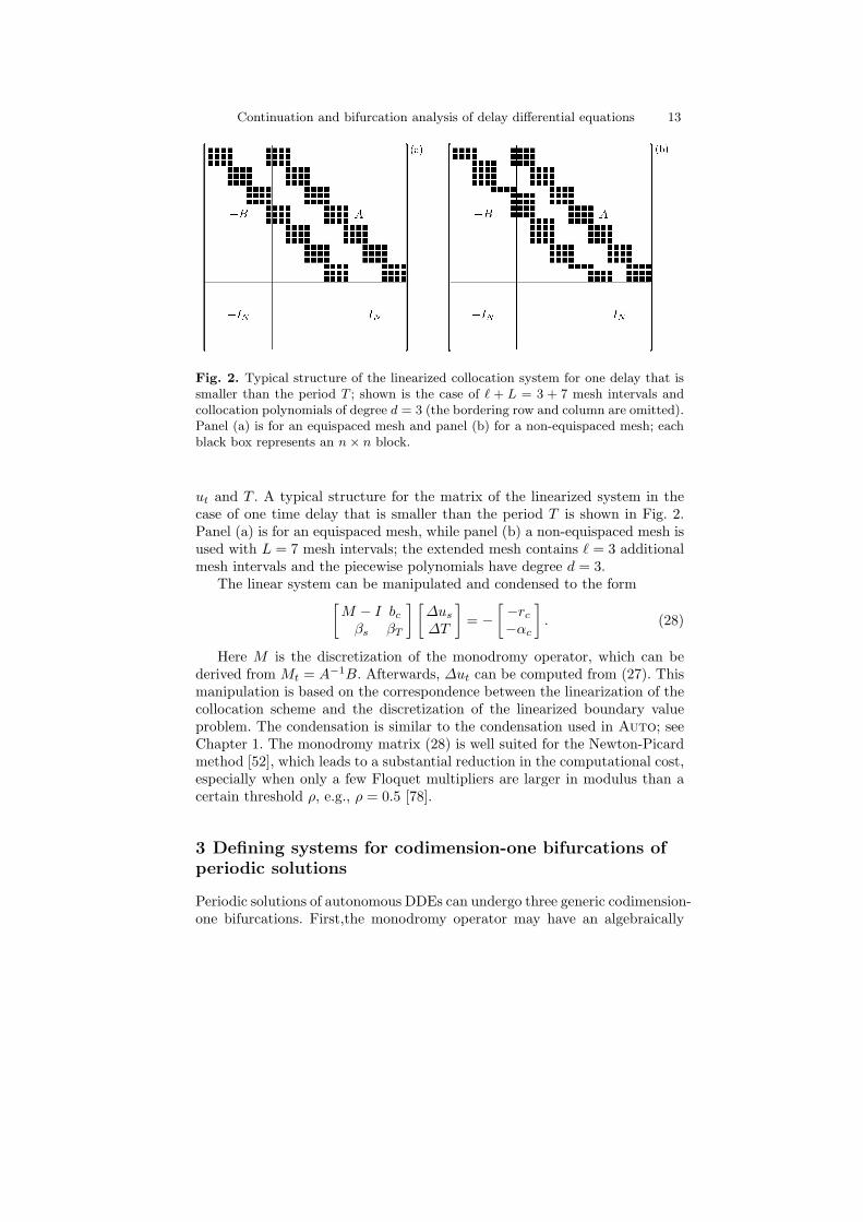
Fig. 2. Typical structure of the linearized collocation system for one delay that issmaller than the period T ; shown is the case of ` + L = 3 + 7 mesh intervals andcollocation polynomials of degree d = 3 (the bordering row and column are omitted).Panel (a) is for an equispaced mesh and panel (b) for a non-equispaced mesh; eachblack box represents an n× n block.

ut and T . A typical structure for the matrix of the linearized system in thecase of one time delay that is smaller than the period T is shown in Fig. 2.Panel (a) is for an equispaced mesh, while panel (b) a non-equispaced mesh isused with L = 7 mesh intervals; the extended mesh contains ` = 3 additionalmesh intervals and the piecewise polynomials have degree d = 3.

The linear system can be manipulated and condensed to the form[M − I bcβs βT

] [∆us∆T

]= −

[ −rc−αc

]. (28)

Here M is the discretization of the monodromy operator, which can bederived from Mt = A−1B. Afterwards, ∆ut can be computed from (27). Thismanipulation is based on the correspondence between the linearization of thecollocation scheme and the discretization of the linearized boundary valueproblem. The condensation is similar to the condensation used in Auto; seeChapter 1. The monodromy matrix (28) is well suited for the Newton-Picardmethod [52], which leads to a substantial reduction in the computational cost,especially when only a few Floquet multipliers are larger in modulus than acertain threshold ρ, e.g., ρ = 0.5 [78].

3 Defining systems for codimension-one bifurcations ofperiodic solutions

Periodic solutions of autonomous DDEs can undergo three generic codimension-one bifurcations. First,the monodromy operator may have an algebraically


double +1 eigenvalue, which corresponds to a limit point (or fold, or saddle-node) bifurcations where the solution ceases to exist. Secondl, there may be asingle −1 multiplier, which gives a period-doubling bifurcation. Third, if twocritical complex conjugate multipliers lie on the unit circle of the complexplane, then there is a Neimark-Sacker or torus bifurcation. In this case aninvariant torus bifurcates from the periodic solution.

Continuing the bifurcations of periodic solutions in DDEs does not differsubstantially from the case of ODEs. In order to compute bifurcations one hasto include additional equations to (20), which are satisfied by a periodic solu-tion if and only if the monodromy operator has a certain kind of singularity.In the period-doubling and the Neimark-Sacker cases, the simplest procedureto construct such a determining system is to require that the monodromy op-erator has a singular vector. Short algebraic transformations of (24) revealsthat these bifurcations occur if

A −

N∑

j=1

σjBj

v = 0,

v?v = 1, (29)

has a unique solution v with the inverse characteristic multiplier σ = µ−1 6= 1on the unit circle. Because of the appearance of higher powers of σ, this equa-tion is different from the ODE case if the delay is larger than the period.Adding (29) to the defining system of the periodic solution (20) doubles thesize of the problem. The size of (29) can be reduced to n+1 by using charac-teristic matrices that are equivalent to the operator in (29) [75]. However, thesmallest possible addition would consist of only one additional scalar equationto (20) without introducing new variables. This can be achieved by using thebordering theorem [8], which states that the bordered operator

(D βα? δ

)=

(A bc? 0

)−1

,

exists if both A and A∗ have one-dimensional kernels and b /∈ kerA∗, c /∈ kerAor A is bijective and c?A−1b 6= 0. Moreover, δ can be used as a test functionalof the singularity, because it is zero if and only if A is singular. In order toobtain δ it is sufficient to solve the equation

(A bc? 0

)(βδ

)=

(01

). (30)

Hence, using a discretized version of A−∑Nj=1 σ

jBj for the operator A in(30) with appropriate choices of b and c? in the period-doubling and Neimark-Sacker case, the equation δ(x∗, η) = 0 determines the bifurcation point. In acontinuation context the resulting β can be re-used as the value of c in thenext continuation step. Similarly, by solving the adjoint equation


(A? cb? 0

)(αδ

)=

(01

),

the resulting α can be the new value of b in the next continuation step.In the case of the fold bifurcation in an autonomous system (1), because

of the algebraically double +1 multiplier, the operator A has to be

ALP =( A −∑N

j=1 σjBj φ0

Intψ0 0

),

where

ψ0 = f(x(t), x(t− τ1), x(t− τ2), . . . , x(t− τm), η),

φ0 = −N∑

j=1

jBjψ0

and

Intψ0 φ =∫ 0

−1

ψ0(θ)φ(θ)dθ.

Note that ALP is different from what one would expect by analogy with ODEs;see [19]. Here, φ0 is obtained by computing the Jordan chain of A−∑N

j=1 σjBj ;

see, e.g., [46]. The regularity of δ obtained from ALP at the bifurcation pointcan be proven either by using the equivalence with characteristic matrices [75]or by standard techniques [19].

4 Connecting orbits

A solution x?(t) of (1) at some fixed value of the parameter η is called aconnecting orbit if the limits

limt→−∞

x?(t) = x− and limt→+∞

x?(t) = x+ (31)

exist, where x− and x+ are steady states of (1). We call the orbit homoclinicwhen x− = x+, and heteroclinic otherwise. Orbits of this type exist, for in-stance, in lasers models with optical feedback, which are discussed in Sec. 8.1;see also [34]. They also appear naturally when looking for traveling waves indelay partial differential equations [66].

A defining condition for a connecting orbit is that it is contained in boththe stable manifold of x+ and the unstable manifold of x−. A classical ap-proach in the ODE case is to approximate this condition by truncating thetime domain to an interval of length Tc and to apply (so-called) projectionboundary conditions [7]: one end point of the connecting orbit is required tolie in the unstable eigenspace of x− and the other end point in the stable


eigenspace of x+. The projection boundary conditions, therefore, replace thestable and unstable manifolds by their linear approximations near the steadystates.

Here, the boundary conditions need to be written in terms of solutionsegments. Furthermore, x+ has infinitely many eigenvalues with negative realparts (see Sec. 1) and so it is impossible to write the final function segmentas a linear combination of all stable eigenfunctions. Instead, it is requiredthat the end function segment is in the orthogonal complement of all unstableleft eigenfunctions. We will assume for notational convenience that (1) onlycontains one delay τ ; however, the method is implemented in DDE-Biftoolfor the general case of m fixed delays.

The condition for the initial function segment x0(θ) can be written as

x0(θ) = x− + ε

s−∑

k=1

αkv−k e

λ−k θ(∑

|αk|2 = 1),

where s− is the number of unstable eigenvalues λ−, with corresponding ei-genvectors v−. The αk are unknown coefficients, and ε is a measure for thedesired accuracy. An extra condition is added to ensure continuity at θ = 0.Since we cannot write the end conditions for the final function segment in asimilar way, a special bilinear form [36] is used to express the fact that thefinal function segment is in the complement of the unstable eigenspace of x+.This leads to the s+ extra conditions of the form

w+k

∗(x(Tc)− x+) +

∫ 0

−τw+k

∗e−λ

+k (θ+τ)A1(x+, η)

(x(Tc + θ)− x+

)dθ = 0 ,

where k = 1, . . . , s+. Here s+ is the number of unstable eigenvalues of x+, w+k

are the left eigenvectors corresponding to the eigenvalues λ+k , and the matrix

A1 is defined as in (3). While this integral condition works well in practice,one slight drawback is that it does not control the distance of the end functionsegment to the steady state.

As for periodic solutions, connecting orbits arise in one-parameter familiesand any time-translate is also a connecting orbit. Therefore, a phase conditionsuch as (14) needs to be added to select one of these orbits.

For the case of a one-parameter family of connecting orbits a number offree parameters are required to obtain a generically isolated solution. Onehas to solve (1) together with the steady-state equations (2) for x− and x+

and characteristic equations of the form (8) for λ−k and v−k and λ+k and w+

k ,i.e., a system of n differential equations, supplemented with (s− + s+)(n +1) + 2n+ s+ + 2 extra equations, resulting in the need for sη = s+ − s− + 1free parameters. This leads to a boundary value problem, which is coupled toa number of algebraic constraints for the equilibria and their stability. Theboundary value problem can be solved by a collocation method as in Sec. 2.1.

Good starting conditions for Newton’s method can be obtained as fol-lows. For a homoclinic orbit, one can start from a nearby periodic solution


with a sufficiently large period. Heteroclinic orbits can be approximated byusing time integration or by using an extension of the method of successivecontinuation [18]. Details of the method, including a numerical study of theconvergence, are presented in [65].

5 Quasiperiodic tori

In dynamical systems quasiperiodic solutions reside on invariant tori. In thissection we describe a method to compute two-dimensional tori as periodicfunctions on the unit square. In particular we adapt the method of Schilderet al. [67], which uses a finite difference method to discretize the definingequation. Here we use a spectral collocation method that is well suited todelay equations.

A quasiperiodic solution x(t) of (1) has two rationally independent fre-quencies ω1, ω2. Hence, there exists a function y : R2 → Rn, which is 2π-periodic in both variables, such that x can be written as x(t) = y(ω1t1, ω2t2).Putting y into (1) yields a first order delayed partial differential equation

∂

∂t1y(t1, t2) +

ω2

ω1

∂

∂t2y(t1, t2) =

1ω1f(y(t1, t2), y(t1 − ω1τ1, t2 − ω2τ1), . . .

. . . , y(t1 − ω1τm, t2 − ω2τm), η), (32)

where ω1, ω2 are unknown frequencies. Because there are translational sym-metries in both variables of y, two phase conditions have to be imposed ony in order to fix a unique solution and determine the unknown frequencies.Assuming that we have a reference solution u(0) of (32) at η0, we formulate acondition that minimizes the distance of u at η from u(0), i.e.,

κ(θ1, θ2) =1

(2π)2

∫ 2π

0

∫ 2π

0

‖u(t1 + θ1, t2 + θ2)− u(0)(t1, t2)‖22dt1dt2.

Taking the first derivative of κ with respect to θ1 and θ2, the phase conditionsbecome

1(2π)2

∫ 2π

0

∫ 2π

0

∂

∂t1u(0)(t1, t2)u(t1, t2)dt1dt2 = 0,

1(2π)2

∫ 2π

0

∫ 2π

0

∂

∂t2u(0)(t1, t2)u(t1, t2)dt1dt2 = 0.

In the case of time periodic systems only the second phase condition is ne-cessary, since the phase in t1 is fixed by the phase of the forcing. In additionto the phase conditions, we also need boundary conditions that guarantee theperiodicity of u, that is,

u(0, t2) = y(2π, t2) andu(t1, 0) = y(t1, 2π), ∀ t1, t2 ∈ [0, 2π].


5.1 Spectral collocation

To obtain an approximation of the quasiperiodic solution the defining sets ofequations can be solved with an appropriate numerical scheme and Newton’smethod. There are several different spectral collocation methods for partialdifferential equations that could be used to solve (32); for an introduction seeTrefethen [76]. Here we use a method that was developed for computation-ally challenging hyperbolic equations such as the Navier-Stokes equation. Themethod is a multi-domain spectral collocation method called the staggeredgrid Chebyshev method, developed by Kopriva and Kolias [48].

The method is similar to the collocation of periodic solutions. It usespiecewise polynomials that are represented by their values at discrete pointsof a mesh, which is different from the mesh on which the equation is solved.We use a very simple domain subdivision of the area [0, 2π]× [0, 2π] that splitsit into the rectangles

Di,j = [ti1, ti+11 ]× [tj2, t

j+12 ],

where 0 = t0l < t1l < · · · < tLl

l = 2π with l ∈ 1, 2. On each rectangle Di,j

we use the Lobatto points (ti,p1 , tj,q2 ) = (ti1+bp1(ti+11 −ti+1

1 ), ti2+bq2(tj+12 −tj+1

2 ))to represent the solution

u(t1, t2) =d1∑p=0

d2∑q=0

u(ti,p1 , tj,q1 )P i,j,p,q(t1, t2), (33)

where P i,j,p,q are the Lagrange polynomials through the points (ti,p1 , tj,q2 ). Thefunction u is now completely determined by the values

ui,j,p,q := u(ti,p1 , tj,q1 ),

which we consider identical if they represent the same point in [0, 2π]× [0, 2π].We also need to impose the boundary conditions, which are

u0,j,0,q = uL1−1,j,d1,q, 0 6 q < d2, 0 6 j < L2 − 1ui,0,p,0 = ui,L2−1,p,d2 , 0 6 p < d1, 0 6 i < L1 − 1 and (34)u0,0,0,0 = uL1−1,L2−1,d1,d2 .

It is also possible to think of the piecewise polynomials as discontinuous in theinterfaces and define mortar equations as in spectral penalty methods (see,e.g., Hesthaven [43]) instead of (34).

Equation (32) is solved on the grid

(ti,p1 , tj,q2 ) = (ti1 + cq1(tj+11 − tj+1

1 ), ti2 + cq2(tj+12 − tj+1

2 )),0 6 i < L1, 0 6 j < L2, 0 6 p < d1, 0 6 q < d2,


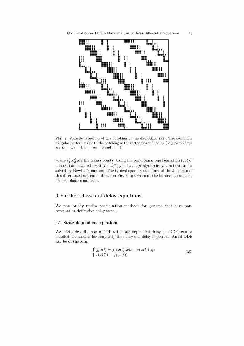
Fig. 3. Sparsity structure of the Jacobian of the discretized (32). The seeminglyirregular pattern is due to the patching of the rectangles defined by (34); parametersare L1 = L2 = 4, d1 = d2 = 3 and n = 1.

where cp1, cq2 are the Gauss points. Using the polynomial representation (33) of

u in (32) and evaluating at (ti,p1 , tj,q2 ) yields a large algebraic system that can besolved by Newton’s method. The typical sparsity structure of the Jacobian ofthis discretized system is shown in Fig. 3, but without the borders accountingfor the phase conditions.

6 Further classes of delay equations

We now briefly review continuation methods for systems that have non-constant or derivative delay terms.

6.1 State dependent equations

We briefly describe how a DDE with state-dependent delay (sd-DDE) can behandled; we assume for simplicity that only one delay is present. An sd-DDEcan be of the form

ddtx(t) = f1(x(t), x(t− τ(x(t)), η)τ(x(t)) = g1(x(t)),

(35)


where g1 : Rn → R is a given (explicit) function of the solution x(t), or it canbe of the form

ddtx(t) = f2(x(t), x(t− τ(t)), τ(t))ddtτ(t) = g2(x(t), x(t− τ(t)), τ(t)),

(36)

where g2 : Rn × Rn × R → R, and the delay is determined by a differentialequation. We assume that all functions in (35) and (36) are sufficiently smoothand that theq delay is bounded, i.e., 0 ≤ τ(t) ≤ r, ∀t. Note that, using x1 ≡ xand x2 ≡ τ , equation (36) can be considered as a particular case of (35) withthe extended state x ≡ (x1, x2).

A steady-state solution of a sd-DDE is determined by the state x andthe delay τ , i.e., the delay should be considered as a part of the solution. Asteady-state solution (x∗, τ∗) of (35) or (36) can be computed by solving a(nonlinear) algebraic system. The local stability of steady-state solutions ofsd-DDEs was studied in [14, 39]. It was shown, under natural assumptionson the right-hand side of the equation and on the delay function τ , thatgenerically the behaviour of the state-dependent delay τ , except for its valueτ∗, has no effect on the stability, and that in the local linearization τ can betreated as a constant. Hence, to study the local stability of a steady stateof (35) or (36), we linearize these equations at x∗ by setting τ ≡ τ∗. Theresulting linearized equation is a DDE with constant delay, and the numericalprocedures discussed in Sec. 1 can be used without changes.

The existence of periodic solutions for particular cases of sd-DDEs has beenstudied by several authors, in particular the existence of ‘slowly oscillatingperiodic solutions’. The theory suggests that a Hopf bifurcation theorem holds;see, e.g., [57]. The stability of periodic solutions has only recently been studied;see, e.g., [40] for non-autonomous sd-DDEs. It was proven that the Frechetderivative of the solution operator of the nonlinear sd-DDE with respect toinitial data equals the solution operator of the linearized equation. Basedon these results we linearize (35) and (36) around a (nonconstant) solution(x∗(t), τ∗(t)) as follows. Let Djfi denote the derivative of f1 with respect toits j-th argument, then

ddty(t) = D1f1(s)y(t)−D2f1(s) d

dtx∗(t− τ(x∗(t))) ∂∂xτ(x

∗(t))y(t)+D2f1(s)y(t− τ(x∗(t)))) (37)

with s = (x∗(t), x∗(t− τ(x∗(t)))), respectively, and

ddty1(t) = D1f2(s)y1(t) +D2f2(s)y1(t− τ∗(t))−D2f2(s) d

dtx∗(t− τ∗(t))y2(t)

+D3f2(s)y2(t)ddty2(t) = D1g2(s)y1(t) +D2g2(s)y1(t− τ∗(t))−D2g2(s) d

dtx∗(t− τ∗(t))y2(t)

+D3g2(s)y2(t)

with s = (x∗(t), x∗(t−τ∗(t)), τ∗(t)). These linearized equations contain a time-dependent (no longer state-dependent) delay. If the coefficients in the linearequation are smooth and periodic (with period T ) and the delay function is


smooth, then the solution operator over the period T (over an interval mT ifτm > T and mT ≥ τm, τm = maxt∈[0,T ] τ(t)) is compact [36].

A periodic solution can be computed by solving a two-point boundaryvalue problem in time, similar to (13), but in case of (36) the additionalequation τ(0) = τ(T ) must be imposed. The solution of these boundary valueproblems by collocation and the computation of the Floquet multipliers isconceptually equal to the procedure outlined in Sec. 2.

6.2 Collocation schemes for equations of neutral type

We summarise basic results on two collocation schemes that were proposed inBarton et. al. [5]. Here we consider the simple equation of neutral type

x(t) = f(x(t), x(t− τ), x(t− τ), η). (38)

The collocation scheme of Sec. 2.1 discretizes (38) by substituting the colloc-ation polynomials and evaluating at the collocation points. In the Jacobianmatrix of this discretized system the second derivatives of the polynomialsappear. This reduces the accuracy by an order, which is only O(hm). Thisdrop in the order of convergence is apparent in the examples of [5]. To rem-edy the situation (38) can be transformed into an ODE coupled to a differenceequation

x(t) = y(t) (39)y(t) = f(x(t), x(t− τ), y(t− τ); (40)

see [5]. Applying the collocation scheme of Sec. 2.1 to this system does notintroduce second order derivatives in the Jacobian matrix and, hence, a betterconvergence can be expected. The numerical experiments in [5] show a con-vergence rate of O(hm+1). In [5] the Gauss-Legendre points were used in thecollocation scheme, together with a periodic boundary condition on the al-gebraic part, but other approaches are possible for delay differential algebraicequations.

7 Software packages

Several software packages exist for simulation (time integration) of delay dif-ferential equations, including ARCHI [62], DKLAG6 [15], RADARS [?] andXPPAUT [28]. Probably the earliest computer program specifically designedfor DDEs has been published by Hassard [41], namely BIFDD which allowsa normal form analysis of Hopf bifurcation points. XPPAUT by Ermentrout[28] allows a limited stability analysis of steady-state solutions of DDEs usingthe approach described in [54].

By contrast, the software packages DDE-Biftool and PDDE-Contimplementnumerical continuation DDEs as introduced in the previous sections. In thissection we describe the functionality of these numerical tools.


7.1 DDE-Biftool

The package DDE-Biftool consists of a collection of Matlab-routines forthe numerical continuation and bifurcation analysis of systems of DDEs withmultiple discrete delays, which may be fixed or state-dependent; for detailedinstructions we refer to the user manual [26]. This software allows one tocompute branches of steady-state solutions and steady-state fold and Hopfbifurcations with continuation. Given an equilibrium, it allows to approxim-ate the right-most, stability-determining roots of the characteristic equation,which can be further corrected with Newton’s method. Periodic solutions andtheir Floquet multipliers can also be computed by collocation with adapt-ive mesh selection. Branches of periodic solutions can be continued startingfrom a previously computed Hopf point or from an initial guess of a peri-odic solution profile. For DDEs with constant delays, also connecting orbits(both homoclinic and heteroclinic solutions) can be computed. The numericalmethods that are used in the software are as detailed in the previous sections.

DDE-Biftool has no graphical user interface, but a number of routinesare provided to plot solution, branch and stability information. Furthermore,automatic detection of bifurcations is not supported. Instead, the evolutionof the characteristic roots or the Floquet multipliers can be computed alongsolution branches, which allows the user to detect and identify bifurcationsusing an appropriate visualisation. Starting points for branch switching atbifurcations on branches of steady-state and periodic solutions can be gener-ated, as well as starting solutions for homoclinic solutions close to periodicsolutions.

Several extensions or ‘add-ons’ have been developed. We mention herea Mathematica program written by Pieroux that allows the automatic gen-eration of the system definition files with symbolically obtained derivatives,software written by Green for the computation of 1D unstable manifolds inDDEs [33], and the extension by Barton for equations of neutral type [5].

7.2 PDDE-Cont

PDDE-Cont implements the numerical methods described in Sec. 2. Itis written in C++ with the use of linear algebraic packages UMFPACK[16],LAPACK [?] and ARPACK [?]. The software has a command line in-terface and a graphical user interface together with a basic plotting facility.

PDDE-Cont can continue periodic solutions of delay equations that arein the form

y′(t) = f(t, y(t), y(t− τ1(t)), y(t− τ2(t)), . . . , y(t− τm(t)), η).

The right-hand side f and the delays τj can be either T -periodic or timeindependent. The software does not have any algorithms to continue equi-libria apart from the obvious fact that an equilibrium can be considered as


a constant periodic solution. Bifurcations of periodic solutions can be con-tinued in two parameters by using test functions as described in Sec. 3, butPDDE-Cont cannot switch branches automatically. For detailed instructionssee the user manual [73]. Note that PDDE-Cont can be used together withDDE-Biftool by converting the results between the two packages.

Due to the low level programming approach, the performance of PDDE-Cont is significantly better than that of DDE-Biftool (which runs underMatlab). Furthermore, PDDE-Cont uses sparse-matrix alogorithms thatrequire less memory, so that problems of relatively high dimension can betackled. The resulting large bordered linear systems (see Sec. 2.1) are solvedby using bordering techniques from [30, 31]. The large sparse matrix withoutborders is factorized by UMFPACK and the whole system is solved using theBEMW method [31].

8 Examples of numerical bifurcation analysis of DDEs

In this section we illustrate the performance of the numerical techniques de-scribed in the previous sections with examples of DDE models of a numberof physical and biological phenomena.

8.1 DDE-PDE model of a laser with optical feedback

A longitudinally single-mode semiconductor laser subject to conventional op-tical feedback and lateral carrier diffusion can be modeled by the hybrid DDE-PDE system

dA(t)dt

= (1− iα)A(t)ζ(t) + ηA(t− τ)e−iφ − ibA(t), (41)

T∂Z(x, t)∂t

= d∂2Z(x, t)∂x2

− Z(x, t) + P (x)

−F (x)(1 + 2Z(x, t))|A(t)|2. (42)

Here the complex scalar variable A(t), represents the amplitude of the elec-trical field E(t) = A(t)eibt, and real Z(x, t),x ∈ [−0.5, 0.5], represents thecarrier density [77], The functions ζ(t), P (x) and F (x) are specified in [77].Continuous-wave solutions, called ‘external cavity modes’ (ECMs) can becomputed as steady-state solutions of (41)–(42), augmented with a scalarcondition for the unknown b and an extra scalar constraint to remove theS1-symmetry. Zero Neumann boundary conditions for Z(x, t) are imposed atx = ±0.5. In the computations the time variable is rescaled so that one timeunit represents 1/1000 of a second. NOTE: this must be checked !!! Thesymmetry about x = 0 is exploited by considering only the interval [0, 0.5].Splitting (41) into real and imaginary part and discretizing (42) in space witha second order central difference formula with constant stepsize∆x = 0.5/128.


0 1 2 3 4 5 6 7

x 10−3

3.2

3.25

3.3

3.35

3.4

η

Inte

nsity

(|A

|2 )

Fig. 4. Bifurcation diagram in the plane of intensity |A|2 vs. feedback strength η ofsteady-state solutions of (41)–(42) for α = 3, φ = 0, T = 1000, d = 1.68× 10−2 andτ = 1000. Stable solutions are drawn as solid curves and unstable solutions as dashedcurves; also shown are saddle-node bifurcations (×) and Hopf bifurcations(*). Re-produced from K. Verheyden, K. Green, and D. Roose, Numerical stability analysisof a large-scale delay system modeling a lateral semiconductor laser subject to op-tical feedback, Phys. Rev. Lett. 69(3) (2004) 036702 c© 2004, with permission fromthe American Physical Society.

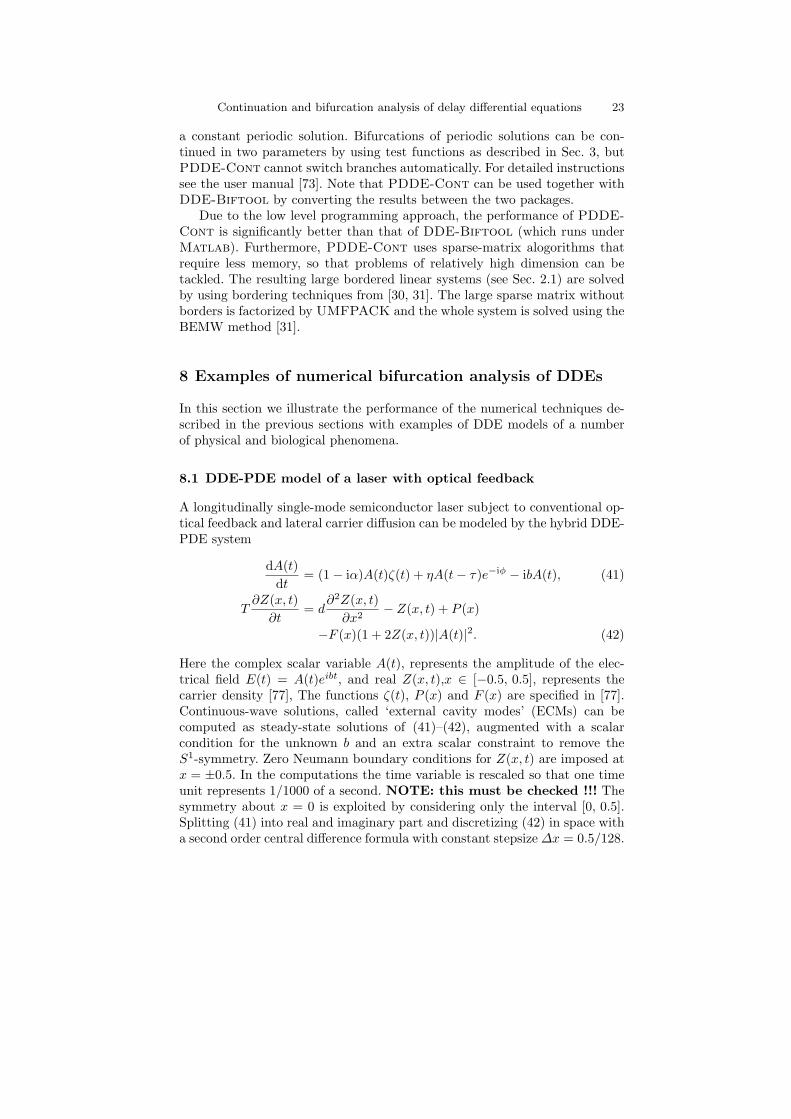
Figure 4 shows the bifurcation diagram of steady-state solutions of (41)–(42) with α = 3, φ = 0, T = 1000, d = 1.68× 10−2 and τ = 1000, obtained bycontinuation with DDE-Biftool, with the feedback strength η as the para-meter. The diagram shows several branches of steady-state solutions arisingfrom saddle-node bifurcations. During continuation the right-most character-istic roots are computed and monitored, allowing for the detection of Hopfbifurcation points along these branches.

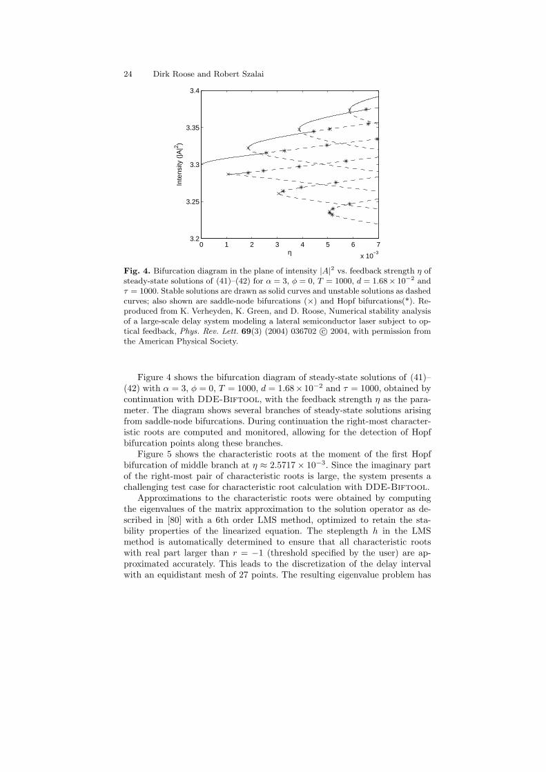
Figure 5 shows the characteristic roots at the moment of the first Hopfbifurcation of middle branch at η ≈ 2.5717× 10−3. Since the imaginary partof the right-most pair of characteristic roots is large, the system presents achallenging test case for characteristic root calculation with DDE-Biftool.

Approximations to the characteristic roots were obtained by computingthe eigenvalues of the matrix approximation to the solution operator as de-scribed in [80] with a 6th order LMS method, optimized to retain the sta-bility properties of the linearized equation. The steplength h in the LMSmethod is automatically determined to ensure that all characteristic rootswith real part larger than r = −1 (threshold specified by the user) are ap-proximated accurately. This leads to the discretization of the delay intervalwith an equidistant mesh of 27 points. The resulting eigenvalue problem has


−6 −4 −2 0

−60

−40

−20

0

20

40

60

Real axisIm

agin

ary

axis

Fig. 5. Characteristic roots at the Hopf point of (41)–(42) η ≈ 2.5717× 10−3 fromFig. 4. Shown are approximations of characteristic roots with real part larger thanr = −1 derived from the eigenvalues of the discretization of the solution operator bythe 6th order special-purpose LMS method (+), and their corrections by Newton’smethod (). Reproduced from K. Verheyden, T. Luzyanina, and D. 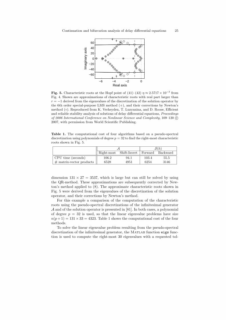Roose, Efficientand reliable stability analysis of solutions of delay differential equations, Proceedingsof 2006 International Conference on Nonlinear Science and Complexity, 109–120 c©2007, with permission from World Scientific Publishing.

Table 1. The computational cost of four algorithms based on a pseudo-spectraldiscretization using polynomials of degree p = 32 to find the right-most characteristicroots shown in Fig. 5.

A S(h)Right-most Shift-Invert Forward Backward

CPU time (seconds) 106.2 94.1 103.4 55.5# matrix-vector products 6528 4951 6254 3146

dimension 131 × 27 = 3537, which is large but can still be solved by usingthe QR-method. These approximations are subsequently corrected by New-ton’s method applied to (8). The approximate characteristic roots shown inFig. 5 were derived from the eigenvalues of the discretization of the solutionoperator, and their corrections by Newton’s method.

For this example a comparison of the computation of the characteristicroots using the pseudo-spectral discretizations of the infinitesimal generatorA and of the solution operator is presented in [81]. In both cases, a polynomialof degree p = 32 is used, so that the linear eigenvalue problems have sizen(p+1) = 131× 33 = 4323. Table 1 shows the computational cost of the fourmethods.

To solve the linear eigenvalue problem resulting from the pseudo-spectraldiscretization of the infinitesimal generator, the Matlab function eigs func-tion is used to compute the right-most 30 eigenvalues with a requested tol-


erance of 10−8 (results indicated with ‘Right-most’). Note that eigs usesArnoldi’s method with implicit restart, and this method does not requirethe explicit construction of the matrix. For the results indicated with ‘Shift-Invert’, eigs is used in conjunction with the shift-invert technique and returnsthe eigenvalues λ closest to the shift ‖A0‖+‖A1‖ ≈ 4528.5, as proposed in [9].The pseudo-spectral discretization of the solution operator S(h) leads to twoalgorithms, called forward and backward variants in [81]. The steplength h ischosen to be 10−4 for the forward and 10−3 for the backward variant, respect-ively.

The accuracy of the computed characteristic roots is similar for the fourmethods. For example, the roots −0.285 ± i11.8 are computed by the fouralgorithms with a relative error between 6.5 10−12 and 2.4 10−14. The accuracyis lower for the eigenvalues with large imaginary part (the relative error onthe pure imaginary eigenvalues ±i47.7 is ≈ 10−4 for the backward variant,and ≈ 7 10−6 for the three other algorithms. The exponential convergencewith respect to the degree p has been confirmed by numerical experiments.

8.2 The Mackey-Glass equation

The equation

x(t) = ax(t) + bx(t− τ)

1 + x10(t− τ). (43)

models the regeneration of white blood cells [55], and it is today widely knownas the Mackey-Glass equation. Although it is a simple equation, not much isknown about its solution structure.

The three equilibria of (43), i.e., x1 = 0 and x2,3 = 10√−(a+ b)/a are

connected to each other at a = −b by a supercritical pitchfork bifurcation.The nonzero solutions can lose their stability in a Hopf bifurcation along thecurves in parameter space given by

a = − arccos(−d−1)1

τ√d2 − 1

,

b =10ad− 9

,

where |d| ≥ 1. Hopf bifurcations for d > 1 are supercritical, so they give rise tostable periodic solutions. These periodic solutions bifurcate further of severalperiod doublings, which then leads to chaotic motion. It was demonstrated in[37] that chaos arises due to the transverse intersection of the two-dimensionalunstable and infinite dimensional stable manifold of this periodic solution. Weremark that some square shaped solutions of large period can be obtained bysingularly perturing a map to give

εx(t) = ax(t) + bx(t− 1)

1 + xc(t− 1),

where ε→ 0 and ετ = 1; see [56] for details.


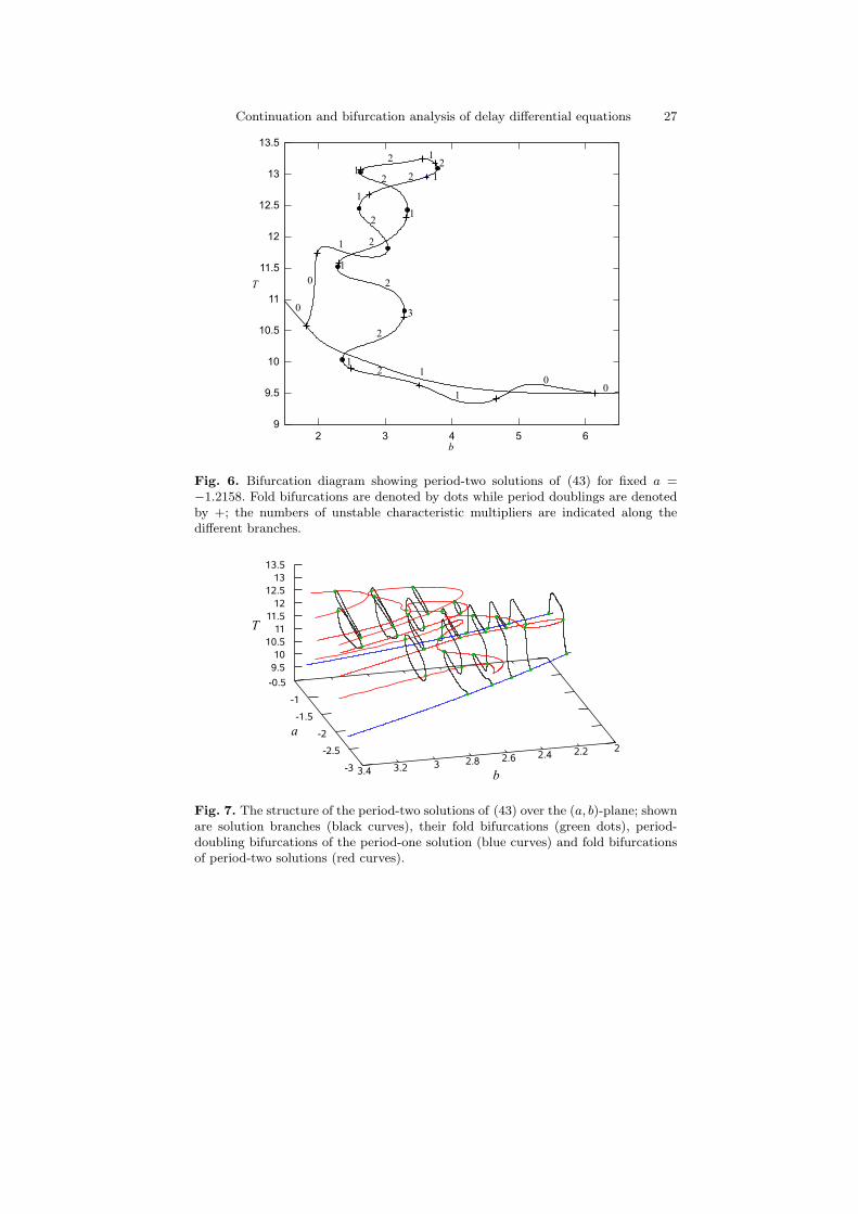
Fig. 6. Bifurcation diagram showing period-two solutions of (43) for fixed a =−1.2158. Fold bifurcations are denoted by dots while period doublings are denotedby +; the numbers of unstable characteristic multipliers are indicated along thedifferent branches.

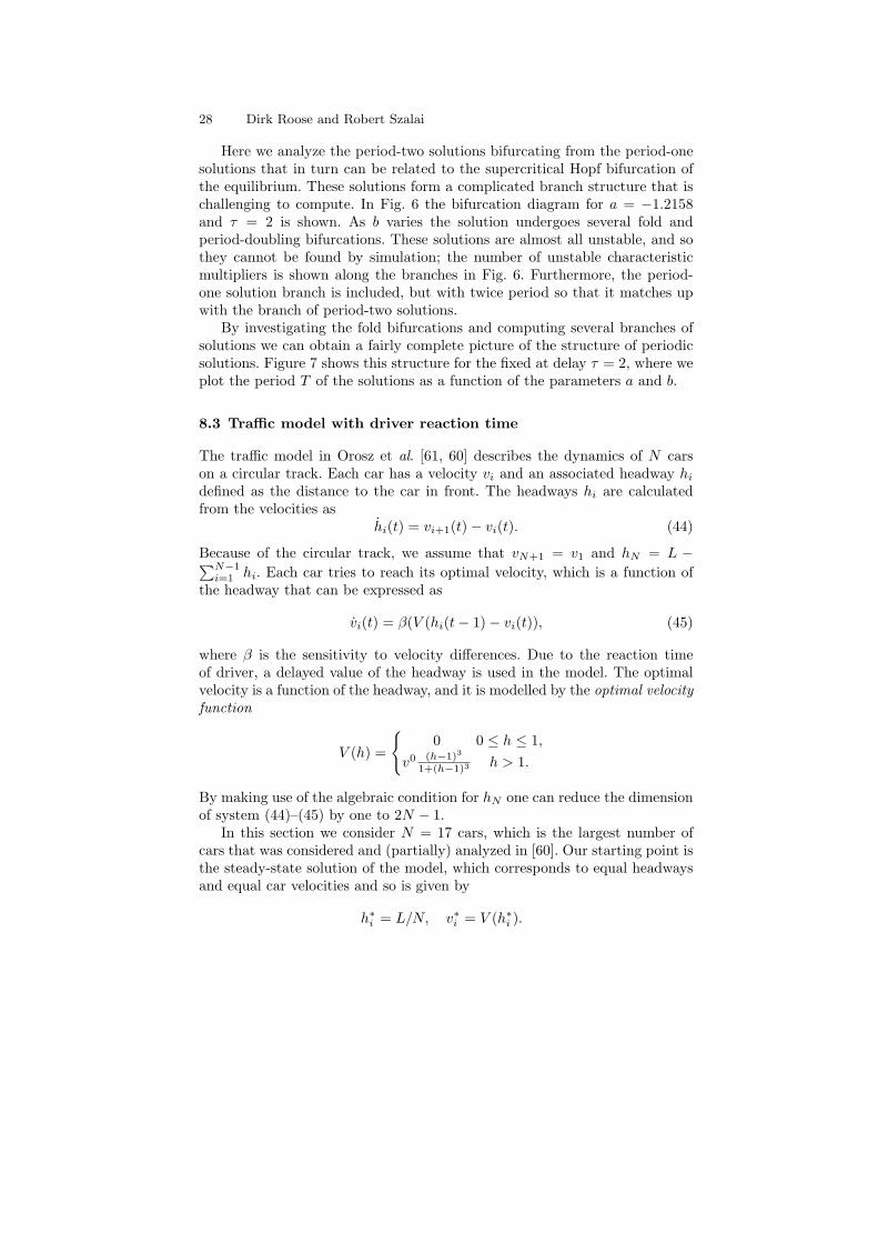
Fig. 7. The structure of the period-two solutions of (43) over the (a, b)-plane; shownare solution branches (black curves), their fold bifurcations (green dots), period-doubling bifurcations of the period-one solution (blue curves) and fold bifurcationsof period-two solutions (red curves).


Here we analyze the period-two solutions bifurcating from the period-onesolutions that in turn can be related to the supercritical Hopf bifurcation ofthe equilibrium. These solutions form a complicated branch structure that ischallenging to compute. In Fig. 6 the bifurcation diagram for a = −1.2158and τ = 2 is shown. As b varies the solution undergoes several fold andperiod-doubling bifurcations. These solutions are almost all unstable, and sothey cannot be found by simulation; the number of unstable characteristicmultipliers is shown along the branches in Fig. 6. Furthermore, the period-one solution branch is included, but with twice period so that it matches upwith the branch of period-two solutions.

By investigating the fold bifurcations and computing several branches ofsolutions we can obtain a fairly complete picture of the structure of periodicsolutions. Figure 7 shows this structure for the fixed at delay τ = 2, where weplot the period T of the solutions as a function of the parameters a and b.

8.3 Traffic model with driver reaction time

The traffic model in Orosz et al. [61, 60] describes the dynamics of N carson a circular track. Each car has a velocity vi and an associated headway hidefined as the distance to the car in front. The headways hi are calculatedfrom the velocities as

hi(t) = vi+1(t)− vi(t). (44)

Because of the circular track, we assume that vN+1 = v1 and hN = L −∑N−1i=1 hi. Each car tries to reach its optimal velocity, which is a function of

the headway that can be expressed as

vi(t) = β(V (hi(t− 1)− vi(t)), (45)

where β is the sensitivity to velocity differences. Due to the reaction timeof driver, a delayed value of the headway is used in the model. The optimalvelocity is a function of the headway, and it is modelled by the optimal velocityfunction

V (h) =

0 0 ≤ h ≤ 1,

v0 (h−1)3

1+(h−1)3 h > 1.

By making use of the algebraic condition for hN one can reduce the dimensionof system (44)–(45) by one to 2N − 1.

In this section we consider N = 17 cars, which is the largest number ofcars that was considered and (partially) analyzed in [60]. Our starting point isthe steady-state solution of the model, which corresponds to equal headwaysand equal car velocities and so is given by

h∗i = L/N, v∗i = V (h∗i ).


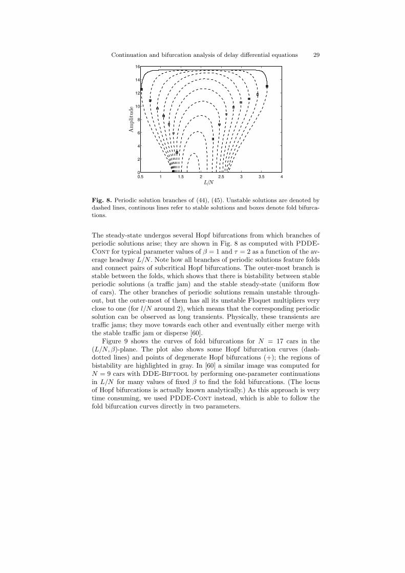
Fig. 8. Periodic solution branches of (44), (45). Unstable solutions are denoted bydashed lines, continous lines refer to stable solutions and boxes denote fold bifurca-tions.

The steady-state undergos several Hopf bifurcations from which branches ofperiodic solutions arise; they are shown in Fig. 8 as computed with PDDE-Cont for typical parameter values of β = 1 and τ = 2 as a function of the av-erage headway L/N . Note how all branches of periodic solutions feature foldsand connect pairs of subcritical Hopf bifurcations. The outer-most branch isstable between the folds, which shows that there is bistability between stableperiodic solutions (a traffic jam) and the stable steady-state (uniform flowof cars). The other branches of periodic solutions remain unstable through-out, but the outer-most of them has all its unstable Floquet multipliers veryclose to one (for l/N around 2), which means that the corresponding periodicsolution can be observed as long transients. Physically, these transients aretraffic jams; they move towards each other and eventually either merge withthe stable traffic jam or disperse [60].

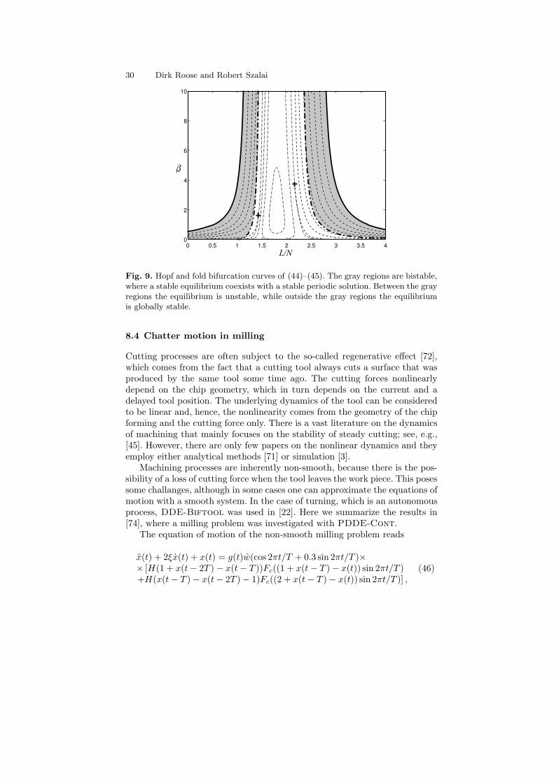
Figure 9 shows the curves of fold bifurcations for N = 17 cars in the(L/N, β)-plane. The plot also shows some Hopf bifurcation curves (dash-dotted lines) and points of degenerate Hopf bifurcations (+); the regions ofbistability are highlighted in gray. In [60] a similar image was computed forN = 9 cars with DDE-Biftool by performing one-parameter continuationsin L/N for many values of fixed β to find the fold bifurcations. (The locusof Hopf bifurcations is actually known analytically.) As this approach is verytime consuming, we used PDDE-Cont instead, which is able to follow thefold bifurcation curves directly in two parameters.


Fig. 9. Hopf and fold bifurcation curves of (44)–(45). The gray regions are bistable,where a stable equilibrium coexists with a stable periodic solution. Between the grayregions the equilibrium is unstable, while outside the gray regions the equilibriumis globally stable.

8.4 Chatter motion in milling

Cutting processes are often subject to the so-called regenerative effect [72],which comes from the fact that a cutting tool always cuts a surface that wasproduced by the same tool some time ago. The cutting forces nonlinearlydepend on the chip geometry, which in turn depends on the current and adelayed tool position. The underlying dynamics of the tool can be consideredto be linear and, hence, the nonlinearity comes from the geometry of the chipforming and the cutting force only. There is a vast literature on the dynamicsof machining that mainly focuses on the stability of steady cutting; see, e.g.,[45]. However, there are only few papers on the nonlinear dynamics and theyemploy either analytical methods [71] or simulation [3].

Machining processes are inherently non-smooth, because there is the pos-sibility of a loss of cutting force when the tool leaves the work piece. This posessome challanges, although in some cases one can approximate the equations ofmotion with a smooth system. In the case of turning, which is an autonomousprocess, DDE-Biftool was used in [22]. Here we summarize the results in[74], where a milling problem was investigated with PDDE-Cont.

The equation of motion of the non-smooth milling problem reads

x(t) + 2ξx(t) + x(t) = g(t)w(cos 2πt/T + 0.3 sin 2πt/T )×× [H(1 + x(t− 2T )− x(t− T ))Fc((1 + x(t− T )− x(t)) sin 2πt/T )+H(x(t− T )− x(t− 2T )− 1)Fc((2 + x(t− T )− x(t)) sin 2πt/T )] ,

(46)


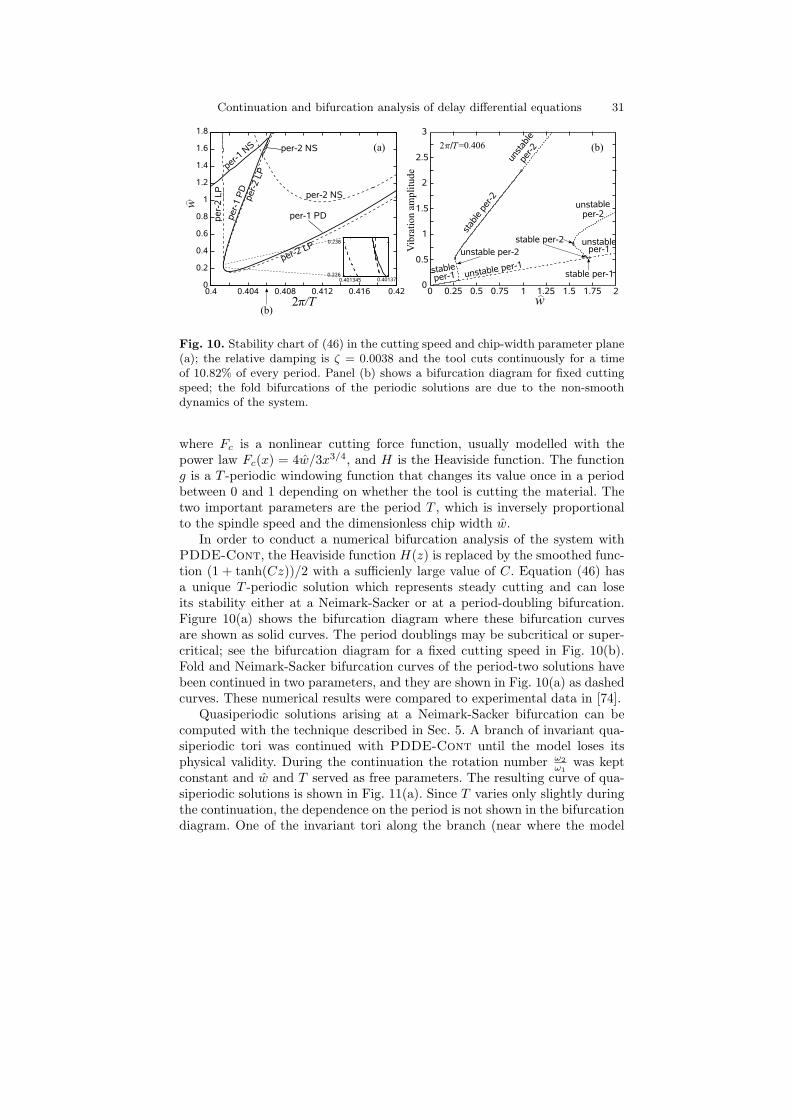
Fig. 10. Stability chart of (46) in the cutting speed and chip-width parameter plane(a); the relative damping is ζ = 0.0038 and the tool cuts continuously for a timeof 10.82% of every period. Panel (b) shows a bifurcation diagram for fixed cuttingspeed; the fold bifurcations of the periodic solutions are due to the non-smoothdynamics of the system.

where Fc is a nonlinear cutting force function, usually modelled with thepower law Fc(x) = 4w/3x3/4, and H is the Heaviside function. The functiong is a T -periodic windowing function that changes its value once in a periodbetween 0 and 1 depending on whether the tool is cutting the material. Thetwo important parameters are the period T , which is inversely proportionalto the spindle speed and the dimensionless chip width w.

In order to conduct a numerical bifurcation analysis of the system withPDDE-Cont, the Heaviside function H(z) is replaced by the smoothed func-tion (1 + tanh(Cz))/2 with a sufficienly large value of C. Equation (46) hasa unique T -periodic solution which represents steady cutting and can loseits stability either at a Neimark-Sacker or at a period-doubling bifurcation.Figure 10(a) shows the bifurcation diagram where these bifurcation curvesare shown as solid curves. The period doublings may be subcritical or super-critical; see the bifurcation diagram for a fixed cutting speed in Fig. 10(b).Fold and Neimark-Sacker bifurcation curves of the period-two solutions havebeen continued in two parameters, and they are shown in Fig. 10(a) as dashedcurves. These numerical results were compared to experimental data in [74].

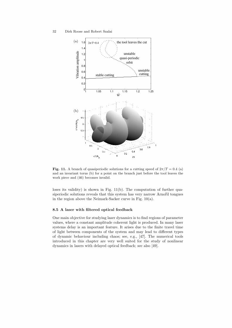
Quasiperiodic solutions arising at a Neimark-Sacker bifurcation can becomputed with the technique described in Sec. 5. A branch of invariant qua-siperiodic tori was continued with PDDE-Cont until the model loses itsphysical validity. During the continuation the rotation number ω2

ω1was kept

constant and w and T served as free parameters. The resulting curve of qua-siperiodic solutions is shown in Fig. 11(a). Since T varies only slightly duringthe continuation, the dependence on the period is not shown in the bifurcationdiagram. One of the invariant tori along the branch (near where the model


(a)

(b)

Fig. 11. A branch of quasiperiodic solutions for a cutting speed of 2π/T = 0.4 (a)and an invariant torus (b) for a point on the branch just before the tool leaves thework piece and (46) becomes invalid.

loses its validity) is shown in Fig. 11(b). The computation of further qua-siperiodic solutions reveals that this system has very narrow Arnol′d tonguesin the region above the Neimark-Sacker curve in Fig. 10(a).

8.5 A laser with filtered optical feedback

One main objective for studying laser dynamics is to find regions of parametervalues, where a constant amplitude coherent light is produced. In many lasersystems delay is an important feature. It arises due to the finite travel timeof light between components of the system and may lead to different typesof dynamic behaviour including chaos; see, e.g., [47]. The numerical toolsintroduced in this chapter are very well suited for the study of nonlineardynamics in lasers with delayed optical feedback; see also [49].


In this section we summarize some results of Erzgraber et. al. [29], who in-vestigate a DDE model of a semiconductor laser with filtered optical feedbackof the form

dEdt

= (1 + iα)N(t) + κF (t), (47)

TdNdt

= P −N(t)− (1 + 2N(t))|E(t)|2, (48)

dFdt

= ΛE(t− τ)e−iCp + (i∆− Λ)F (t), (49)

where the variable E is the complex optical field, N is the (real-valued) pop-ulation inversion of the laser, and F is the complex optical field of the filter.The material properties of the laser are given by the linewidth enhancementfactor α, the electron lifetime T and the pump rate P . The coupling of thelaser with the filter is controlled by the parameter κ, while τ is the time thatthe light spends in the external feedback loop. The dynamics of the filter ismodelled by (49). The feedback phase Cp is the phase difference between thelaser and the filter fields, and ∆ is the detuning between the filter center fre-quency ΩF and the solitary frequency Ω0 of the laser. Hence, Cp = Ω0τ and∆ = ΩF −Ω0.

The laser equations (47)–(49) exhibit a rotational symmetry (rotation ofboth E and F over any angle) that is important for the types of solutions thatare supported. It also needs to be dealt with in the continuation to ensure thatsolutions are isolated. The idea is to consider solutions of the form

(E(t), N(t), F (t)) = (A(t) eibt, N(t), B(t) eib).

By putting this ansatz into (47)–(49) we obtain the new system

dAdt

= (1 + iα)N(t)A(t)− ibA(t) + κB(t) (50)

TdNdt

= P −N(t)− (1 + 2N(t))|A(t)|2, (51)

dBdt

= ΛA(t− τ)e−i(Cp+bτ) + (i∆− Λ− ib)B(t). (52)

Note that the stability of this transformed system does not differ from thethe stability of (47)–(49), because the norm of (E(t), N(t), F (t)) is the sameas the norm of (A(t), N(t), B(t)). System (50)–(52) still has the same rota-tional symmetry, but the equations are now in a form can be dealt with incontinuation.

The primary interest is in the so-called external filtered modes (EFMs),which are single frequency periodic solutions of (50)–(52) that are character-ized by fixed A(t) = As, N(t) = Ns and B(t) = Bs. EFMs were extensivelystudied analytically [59] and with numerical continuation [29]. In order todetermine an EFM uniquely one needs to fix the phase, which can be done,


.

0 0.01 0.02 0.03−4

−2

0

2

4

0

5

−15

0

15

0

2

4

0

5

−3

0

3

0

2

4

0

5

−3

0

3

0

2

4

0 20 40 60−3

0

3

FO

FO

EFMRO

S

S

H

SL

(c)

(b)

DH

DH

T

SL

T

T

T

SL

H

H

(d)SL

H

1:1

1:1

Cp

π

(a)

κ

IL (b1)

ωL (b2)

IF (b3)

IL (c1)

ωL (c2)

IF(c3)

ωF (c4)

t[ns]

IL (d1)

ωL (d2)

IF (d3)

Fig. 12. Panel (a) shows the bifurcation diagram in the (κ, Cp)-plane of (47)–(49)for ∆ = 0, α = 5.0, T = 100, P = 3.5, τ = 500 and Λ = 0.007. EFMs are stable inthe green region, which is bounded by curves of saddle-node bifurcations (blue) andHopf bifurcations (red). Panels (b1)–(b4) show an example of relaxation oscillations,while panels (c1)–(c4) and panels (d1)–(d4) are examples of frequency oscillations;plotted are the laser intensity IL, its frequency ωL, the filter intensity IF , and itsfrequency ωF . The stability regions of the different oscillations are shown in panel(a) in orange, purple and light blue, respectively. Reproduced from H. Erzgraber,B. Krauskopf and D. Lenstra, SIAM J. Appl. Dyn. Sys. 6(1) (2007) ??–?? c© 2007,with permission from the Society for Industrial and Applied Mathematics.

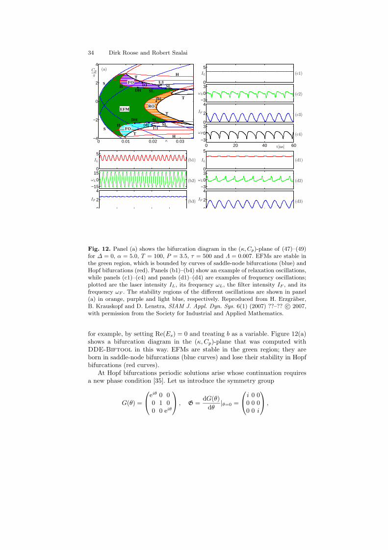
for example, by setting Re(Es) = 0 and treating b as a variable. Figure 12(a)shows a bifurcation diagram in the (κ,Cp)-plane that was computed withDDE-Biftool in this way. EFMs are stable in the green region; they areborn in saddle-node bifurcations (blue curves) and lose their stability in Hopfbifurcations (red curves).

At Hopf bifurcations periodic solutions arise whose continuation requiresa new phase condition [35]. Let us introduce the symmetry group

G(θ) =

eiθ 0 00 1 00 0 eiθ

, G =

dG(θ)dθ

|θ=0 =

i 0 00 0 00 0 i

,


which produces a two-parameter family of solutions

u(t; θ1, θ2) = G(θ1)(A(t+ θ2), N(t+ θ2), B(t+ θ2))

from any solution of (50)–(52). In a continuation context, when looking forthe next solution on a branch of solutions, we want to find the one closestin norm to the previous solution u(0). Hence, the new solution u is chosen tominimize

D(θ1, θ2) =∫ 1

0

‖u(t; θ1, θ2)− u(0)(t))‖22dt

in θ1, θ2. Differentiating with respect to both variables and evaluating at θ1 =θ2 = 0 yields

∫ 1

0

u(0)(s)(u(0)(s)− u(s))ds = 0, (53)∫ 1

0

Gu(0)(s)(u(0)(s)− u(s))ds = 0, (54)

where G = d/dθG(θ)|θ=0 is the infinitesimal generator of the symmetry group.Note that (53) is actually the phase condition (14), while (54) is a new phasecondition that fixes the group invariance.

With (53) and (54) periodic solutions can be continued as isolated solu-tions. These phase conditions are implemented in both DDE-Biftool andPDDE-Cont. In [29] DDE-Biftool was used to compute the periodic solu-tions of (50)–(52) and PDDE-Cont was used to determine their stabilityboundraries by continuing the Neimark-Sacker bifurcation in two parameters.

The resulting stability regions of the two different types of periodic solu-tions are colored in Fig. 12(a), and examples of typical time series are shownin panels (b)–(d). First, there are the typical relaxation oscillations (not tobe confused with relaxation oscillations of slow-fast systems as discussed inChapter 8), which are a periodic exchange of energy between the electric fieldE and the inversion N in a semiconductor lasers. Relaxation oscillations arefast (on the order of a few GHz) and effectively do not involve the filter; seeFig. 12(b). The other type of oscillations are the frequency oscillations, whichare slower and oscillate on the time scale given by the external roundtrip time(that is, the delay τ); see Fig. 12(c) and (d). These oscillations are unusual forsemiconductor lasers because they feature practically constant laser intensityIL but an oscillating frequency ωL. Notice that the dynamics of the filterappears to suppress the dynamics of the intensity. Both types of oscillationslose their stability at Neimark-Sacker bifurcations, which are shown as blackcurves in Fig. 12(a).


9 Conclusions

We discussed numerical continuation methods for the stability and bifurcationanalysis of delay differential equations with constant delays, concentrating ontechniques concerning steady-state solutions and periodic solutions. We alsodescribed how to compute connecting (homoclinic and heteroclinic) orbitsand quasiperiodic solutions. Furthermore, wqe briefly mentioned how to dealwith state dependent delays and with equations of neutral type. Comparedwith numerical methods for such tasks in ordinary differential equations themethods we presented are either similar but with a higher computationalcost (an example is collocation for computing periodic solutions) or muchmore complex (as is the case for computing the stability of a steady state orfinding connected orbit). These additional difficulties are due to the infinite-dimensional nature of DDEs.

Rather than trying to give a complete literature survey, we focused on thenumerical methods implemented in the software packages DDE-Biftool andPDDE-Cont. Both have about the same functionality as similar packagesfor ODEs, but with less flexibility and at a higher computational cost. Theymake continuation and bifurcation analysis for DDEs readily available forscientists dealing with concrete problems arising in applications. We haveincluded results on the continuation and bifurcation analysis of several realisticmodels to illustrate the applicability of the methods.

Numerical developments can also help with the solution of some opentheoretical problems. For example, some numerical results on state-dependentDDEs are ahead of the theory and suggest that certain conditions imposedin the theory are rather technical and not fundamental. One of the areasfor future work for both theory and numerical methods is that of piecewise-smooth delayed systems, which have important applications, for example, incontrol theory [4, 68], hybrid testing [51, 69] and machining [22, ?].

Acknowledgements

We thank Bernd Krauskopf, David Barton, Tatyana Luzyanina, GiovanniSamaey and Koen Verheyden for their useful comments and suggestions. Weare grateful to the American Physical Society, World Scientific Publishingand the Society for Industrial and Applied Mathematics for permission toreproduce Fig. 4, Fig. 5 and Fig. 12, respectively.

References

1. U. M. Ascher, R. M. M. Mattheij, and R. D. Russell. Numerical Solution ofBoundary Value Problems for Ordinary Differential Equations. (Prentice Hall,1988).


2. C. T. H. Baker, C. A. H. Paul, and D. R. Wille. A bibliography on the numericalsolution of delay differential equations. Technical Report 269, University ofManchester, Manchester Centre for Computational Mathematics, 1995.

3. B. Balachandran. Non-linear dynamics of milling process. Trans. Royal Soc.,359:793–820, 2001.

4. D. A. W. Barton, B. Krauskopf, and R. E. Wilson. Explicit periodic solutions ina model of a relay controller with delay and forcing. Nonlinearity, 18(6):2637–2656, 2005.

5. D. A. W. Barton, B. Krauskopf, and R. E. Wilson. Collocation schemes forperiodic solutions of neutral delay differential equations. J. Diff. Eqns. Appl.,12(11):1087-1101, 2006.

6. A. Bellen and M. Zennaro. Numerical Methods for Delay Differential Equations.(Oxford University Press, 2003).

7. W. J. Beyn. The numerical computation of connecting orbits in dynamicalsystems. IMA J. Numer. Analysis, 9:379–405, 1990.

8. W. J. Beyn, A. Champneys, E. J. Doedel, W. Govaerts, B. Sandstede, andY. A. Kuznetsov. Numerical continuation and computation of normal forms. InB. Fiedler, editor, Handbook of Dynamical Systems, pages 149–219. (Elsevier,2002).

9. D. Breda. Numerical computation of characteristic roots for delay differentialequations. PhD thesis (Department of Mathematics and Computer Science,University of Udine, 2004).

10. D. Breda. Solution operator approximation for delay differential equation char-acteristic roots computation via Runge-Kutta methods. Appl. Numer. Math.,56:305–317, 2006.

11. D. Breda, S. Maset, and R. Vermiglio. Computing the characteristic roots fordelay differential equations. IMA J. Numer. Analysis, 24:1–19, 2004.

12. D. Breda, S. Maset, and R. Vermiglio. Pseudospectral differencing methodsfor characteristic roots of delay differential equations. SIAM J. Sci. Comput.,27(2):482–495, 2005.

13. A. M. Castelfranco and H. W. Stech. Periodic solutions in a model of recurrentneural feedback. SIAM J. Appl. Math., 47(3):573–588, 1987.

14. K. L. Cooke and W. Huang. On the problem of linearization for state-dependentdelay differential equations. Proc. Am. Math. Soc., 124(5), 1996.

15. S. P. Corwin, D. Sarafyan, and S. Thompson. DKLAG6: A code based oncontinuously imbedded sixth order Runge-Kutta methods for the solution ofstate dependent functional differential equations. Appl. Numer. Math., 24(2–3):319–330, 1997.

16. T. A. Davies. UMFPACK Version 4.1 User Guide. Technical report, Depart-ment of Computer and Information Science and Engineering, University of Flor-ida, Gainesville, FL, USA, 2003. http://www.cise.ufl.edu/research/sparse/umfpack/.

17. E. J. Doedel, A. R. Champneys, T. F. Fairgrieve, Y. A. Kuznetsov, B. Sandstede,and X. Wang. AUTO97: Continuation and bifurcation software for ordin-ary differential equations, 1997; available via ftp.cs.concordia.ca in directorypub/doedel/auto.

18. E. J. Doedel, M. J. Friedman, and B. I. Kunin. Successive continuation forlocating connecting orbits. Num. Alg., 17:103–124, 1997.


19. E. J. Doedel, W. Govaerts, and Yu. A. Kuznetsov. Continuation of periodicsolution bifurcations in odes using bordered systems. SIAM J. Numer. Analysis,42(2):401–435, 2003.

20. E. J. Doedel, H. B. Keller, and J. P. Kernevez. Numerical analysis and controlof bifurcation problems (II): bifurcations in infinite dimensions. Internat. J.Bifur. Chaos Appl. Sci. Engrg., 1(4):745–772, 1991.

21. E. J. Doedel and P. P. C. Leung. A numerical technique for bifurcation problemsin delay differential equations. Congr. Numer., 34:225–237, 1982. (Proc. 11thManitoba Conf. Num. Math. Comput., Univ. Manitoba, Winnipeg, Canada).

22. Z. Dombovari. Bifurcation analysis of a cutting process. Master’s thesis (Bud-apest University of Technology and Economics, 2006).

23. K. Engelborghs and E. Doedel. Stability of piecewise polynomial collocationfor computing periodic solutions of delay differential equations. Numer. Math.,91(4):627–648, 2002.

24. K. Engelborghs, T. Luzyanina, K. J. in ´t Hout, and D. Roose. Collocationmethods for the computation of periodic solutions of delay differential equations.SIAM J. Sci. Comput., 22(5):1593–1609, 2000.

25. K. Engelborghs, T. Luzyanina, and D. Roose. Numerical bifurcation analysis ofdelay differential equations using DDE-BIFTOOL. ACM Trans. Math. Software,28(1):1–21, 2002.

26. K. Engelborghs, T. Luzyanina, and G. Samaey. DDE-BIFTOOL v. 2.00: a Mat-lab package for bifurcation analysis of delay differential equations. Technical Re-port TW-330, Department of Computer Science, K.U.Leuven, Leuven, Belgium,2001; available at www.cs.kuleuven.ac.be/cwis/research/~twr/research/

software/delay/ddebiftool.shtml.27. K. Engelborghs and D. Roose. On stability of LMS methods and characteristic

roots of delay differential equations. SIAM J. Numer. Analysis, 40(2):629–650,2002.

28. B. Ermentrout. XPPAUT3.91 - The differential equations tool. University ofPittsburgh, Pittsburgh, 1998; available at http://www.pitt.edu/~phase/.

29. H. Erzgraber, B. Krauskopf, and D. Lenstra. Bifurcation analysis of a semicon-ductor laser with filtered optical feedback. SIAM J. Appl. Dyn. Sys., 6(1):??–??,2007.

30. W. Govaerts. Bordered augmented linear systems in numerical continuation andbifurcation. Numer. Math., 58:353–368, 1990.

31. W. Govaerts and J. D. Pryce. Mixed block elimination for linear systems withwider borders. IMA J. of Numer. Analysis, 13:161–180, 1993.

32. K. Green, B. Krauskopf, and K. Engelborghs. Bistability and torus break-up ina semiconductor laser with phase-conjugate feedback. Physica D, 173(1-2):114–129, 2002.

33. K. Green, B. Krauskopf, and K. Engelborghs. One-dimensional unstable eigen-function and manifold computations in delay differential equations. J. Comp.Phys., 197(1):86–98, 2004.

34. K. Green, B. Krauskopf, and G. Samaey. A two-parameter study of the lockingregion of a semiconductor laser subject to phase-conjugate feedback. SIAM J.Appl. Dyn. Sys., 2(2):254–276, 2003.

35. B. Haegeman, K. Engelborghs, D. Roose, D. Pieroux, and T. Erneux. Stabilityand rupture of bifurcation bridges in semiconductor lasers subject to opticalfeedback. Phys. Rev. E, 66:046216 1–11, 2002.


36. J. K. Hale. Theory of Functional Differential Equations, volume 3 of AppliedMathematical Sciences. (Springer-Verlag, New York, 1977).

37. J. K. Hale and N. Sternberg. Onset of chaos in differential delay eqautions. J.Comp. Phys., 77:221–239, 1988.

38. J. K. Hale and S. M. Verduyn Lunel. Introduction to Functional DifferentialEquations, volume 99 of Applied Mathematical Sciences. (Springer-Verlag, NewYork, 1993).

39. F. Hartung and J. Turi. Stability in a class of functional differential equationswith state-dependent delay. In C Corduneanu, editor, Qualitative problems fordifferential equations and control theory, pages 15–31. (World Scientific, Singa-pore, 1995).

40. F. Hartung and J. Turi. On differentiability of solutions with respect to para-meters in state-dependent delay equations. J. Diff. Eqns., 135:192–237, 1997.

41. B. D. Hassard. A code for Hopf bifurcation analysis of autonomous delay-differential systems. In F. V. Atkinson, W. F. Langford, and A. B. Mingarelli,editors, Oscillations, Bifurcations and Chaos, volume 8 of Can. Math. Soc. Con-ference Proceedings, pages 447–463 (Amer. Math. Soc., Providence, RI, 1987).

42. B. D. Hassard. Counting roots of the characteristic equation for linear delay-differential systems. J. Diff. Eqns., 136:222–235, 1997.

43. J. S. Hesthaven. Spectral penalty methods. Appl. Num. Math., 33:23–41, 2000.44. K. J. in ´t Hout and Ch. Lubich. Periodic orbits of delay differential equations

under discretization. BIT, 38(1):72–91, 1998.45. T. Insperger, B. P. Mann, G. Stepan, and P. V. Bayly. Stability of up-milling

and down-milling, part 1: alternative analytical methods. Int. J. of Mach. ToolManuf., 43(1):25–34, 2003.

46. M. A. Kaashoek and S. M. Verduyn Lunel. Characteristic matrices and spectralproperties of evolutionary systems. Trans. Amer. Math. Soc., 334:479–517, 1992.

47. D.M. Kane and K.A. Shore (Eds.), Unlocking Dynamical Diversity: Optical Feed-back Effects on Semiconductor Lasers, (John Wiley & Sons, 2005).

48. D. A. Kopriva and J. H. Kolias. A conservative staggered-grid chebyshev mul-tidomain method for compressible flows. J. Comp. Phys., 125:244–261, 1996.

49. B. Krauskopf. Bifurcation analysis of lasers with delay. In D.M. Kane andK.A. Shore, editors, Unlocking Dynamical Diversity: Optical Feedback Effectson Semiconductor Lasers, pages 147–183. (John Wiley & Sons, 2005).

50. Yu. A. Kuznetsov and V. V. Levitin. CONTENT: A multiplatform environ-ment for analyzing dynamical systems, 1997. Dynamical Systems Laboratory,Centrum voor Wiskunde en Informatica; available via ftp.cwi.nl in directoryurlpub/CONTENT.

51. Y. N. Kyrychko, K. B. Blyuss, A. Gonzalez-Buelga, S. J. Hogan and D. J. Wagg.Real-time dynamic substructuring in a coupled oscillator-pendulum system.Proc. R. Soc. A 462:1271–1294, 2006.

52. K. Lust, D. Roose, A. Spence, and A.R. Champneys. An adaptive Newton-Picard algorithm with subspace iteration for computing periodic solutions.SIAM J. Sci. Comput., 19(4):1188–1209, 1998.

53. T. Luzyanina and K. Engelborghs. Computing Floquet multipliers for functionaldifferential equations. Internat. J. Bif. Chaos Appl. Sci. Engrg., 12(12):2977–2989, 2002.

54. T. Luzyanina and D. Roose. Numerical stability analysis and computation ofHopf bifurcation points for delay differential equations. J. Comput. Appl. Math.,72:379–392, 1996.


55. M. C. Mackey and L. Glass. Oscillation and chaos in physiological controlsystems. Science, 77:287–289, 1977.

56. J. Mallet-Paret and R. D. Nussbaum. A differential delay equation arising inoptics an physiology. SIAM J. Math. Analysis, 20(2):249–292, 1989.

57. J. Mallet-Paret and R.D. Nussbaum. Boundary layer phenomena for differential-delay equations with state-dependent time lags 1. Arch. Rational Mech. Ana-lysis, 120:99–146, 1992.

58. S. I. Niculescu. Delay Effects on Stability: A Robust Control Approach. LectureNotes in Control and Information Science, 269, (Springer-Verlag, New York,2000).

59. M. Nizette and T. Erneux. Optical frequency dynamics and relaxation oscila-tions of a semiconductor laser subject to filtered optical feedback. In M. PessaD. Lenstra and Ian H White, editors, Semiconductor Lasers and Laser DynamicsII, Proceedings of the SPIE, pages 6184–32. 2006.

60. G. Orosz, B. Krauskopf, and R. E. Wilson. Bifurcations and multiple traffic jamsin a car following model with reaction delay time. Physica D, 211:277–293, 2005.

61. G. Orosz, R. E. Wilson, and B. Krauskopf. Global bifurcation investigationof an optimal velocity traffic model with driver reaction time. Phys. Rev. E,70(026207):1–10, 2004.

62. C. A. H. Paul. A user-guide to Archi - an explicit Runge-Kutta code for solvingdelay and neutral differential equations. Technical Report 283 (The Universityof Manchester, Manchester Center for Computational Mathematics, 1997).

63. A. Pazy. Semigroups of linear operators and applications to Partial differentialequations. (Springer-Verlag, New York, 1983).

64. Y. Saad. Iterative Methods for Sparse Systems. (SIAM, Philadelphia, 2003).65. G. Samaey, K. Engelborghs, and D. Roose. Numerical computation of connect-

ing orbits in delay differential equations. Num. Algor., 30(3-4):335–352, 2002.66. G. Samaey and B. Sandstede. Determining stability of pulses for partial differ-

ential equations with time delays. Dyn. Sys., 20(2):201–222, 2005.67. F. Schilder, H. M. Osinga, and W. Vogt. Continuation of quasiperiodic invariant

tori. SIAM J. Appl. Dyn. Sys., 4(3):244–261, 2005.68. J. Sieber. Dynamics of delayed relay systems. Nonlinearity, 19(11):2489–2527,

2006.69. J. Sieber and B. Krauskopf. Control-based bifurcation analysis for experiments.

Nonlin. Dyn. in press.70. G. Stepan. Retarded Dynamical Systems. (Longman, London, 1989).71. G. Stepan and T. Kalmar-Nagy. Nonlinear regenerative machine tool vibrations.

In Proceedings of the 1997 ASME Design Engineering Technical Conferences,Sacramento, California, September 1997. Paper number DETC97/VIB-4021.

72. G. Stepan, R. Szalai, and T. Insperger. Stability of high-speed milling. InG. Radons, editor, Nonlinear Dynamics of Production Systems, pages 111–128.(Wiley VCH, 2003).

73. R. Szalai. PDDE-CONT: A continuation and bifurcation software for delay-differential equations, 2005. Department of Applied Mechanics, BudapestUniversity of Technolgy and Economics; available at http://www.mm.bme.hu/

~szalai/pdde/.74. R. Szalai, B. P. Mann, and G. Stepan. Period-two and quasiperiodic vibrations

of high-speed milling. In I. Grabec and E. Govekar, editors, Proceedings of the9th CIRP International Workshop on Modeling of Machining Operations, pages107–114. CIRP, 2006.


75. R. Szalai, G. Stepan, and S. J. Hogan. Continuation of bifurcations in periodicdelay-differential equations using characteristic matrices. SIAM J. Sci. Comp.,28(4):1301–1317, 2006.

76. L. N. Trefethen. Spectral methods in MATLAB. (SIAM, Philadelphia, 2000).77. K. Verheyden, K. Green, and D. Roose. Numerical stability analysis of a large-

scale delay system modeling a lateral semiconductor laser subject to opticalfeedback. Phys. Rev. E, 69(3):036702, 2004.

78. K. Verheyden and K. Lust. A Newton-Picard collocation method for periodicsolutions of delay differential equations. BIT Num. Math., 45(3):1605–625, 2005.

79. K. Verheyden, T. Luzyanina, and D. Roose. Efficient and reliable stabilityanalysis of solutions of delay differential equations. Proceedings of 2006 In-ternational Conference on Nonlinear Science and Complexity, pages 109–120.(World Scientific Publishing, Singapore, 2006).

80. K. Verheyden, T. Luzyanina, and D. Roose. Efficient computation of character-istic roots of delay differential equations using LMS methods. J. Comp. AppliedMath., 2006. submitted.

81. K. Verheyden and D. Roose. Efficient numerical stability analysis of delayequations: a spectral method. In D. Roose and W. Michiels, editors, Time-delaysystems 2004, IFAC Proceedings Volumes, pages 209–214. (Elsevier, Oxford,UK, 2005).

Date post:	05-Apr-2020
Category:	Documents
Upload:	others
View:	25 times
Download:	0 times

Continuation and bifurcation analysis of delay …kouzn101/rosz.pdfContinuation and bifurcation...

Documents