Continuation-based numerical detection ofafter-depolarisation and spike-adding threshold

Jakub Nowackijakub.nowacki@tessella.comTessella, 26 The Quadrant, Abingdon Science Park, Abingdon, OX14 3YS, UK

Hinke M. Osingah.m.osinga@auckland.ac.nzDepartment of Mathematics,The University of Auckland, Private Bag 92019, Auckland 1142, New Zealand

Krasimira T. Tsaneva-Atanasovak.tsaneva-atanasova@bristol.ac.ukBristol Centre for Applied Nonlinear Mathematics,Department of Engineering Mathematics,University of Bristol, Queen’s Building, University Walk, Bristol BS8 1TR, UK

The changes in neuronal firing pattern are signatures of brain function, and itis of interest to understand how such changes evolve as a function of neuronalbiophysical properties. We address this important problem via the analysis andnumerical investigation of a class of mechanistic mathematical models. We focuson a hippocampal pyramidal neuron model and study the occurrence of burstingrelated to the after-depolarisation (ADP) that follows after a brief current injec-tion. This type of burst is a transient phenomenon, which is not amenable to theclassical bifurcation analysis done, for example, for periodic bursting oscillators.In this paper, we show how to formulate such transient behaviour as a two-pointboundary value problem (2PBVP), which can be solved using well-known con-tinuation methods. The 2PBVP is formulated such that the transient responseis represented by a finite orbit segment for which onsets of ADP and additionalspikes in a burst can be detected as bifurcations during a one-parameter con-tinuation. This, in turn, provides us with a direct method to approximate theboundaries of regions in a two-parameter plane where certain model behaviourof interest occurs. More precisely, we use two-parameter continuation of the de-tected onset points to identify the boundaries between regions with and withoutADP, and bursts with different numbers of spikes. Our 2PBVP formulation is anovel approach to parameter sensitivity analysis that can be applied to a widerange of different problems.

2 J. Nowacki, H.M. Osinga and K.T. Tsaneva-Atanasova

1 Introduction

The firing patterns in neurons are an important feature that is generally associated withspecific brain functions (Llinas, 1988). Under various conditions, many neurons tend to firebursts, i.e., clusters of high-frequency spikes (Krahe & Gabbiani, 2004). Bursts are generatedin response to stimuli, which can be electrical (Yue & Yaari, 2004; Brown & Randall, 2009)or chemical (Rinzel, 1985; Tsaneva-Atanasova, Sherman, van Goor, & Stojilkovic, 2007) andoccur periodically or as single events. The bursting activity is characterised by slow alter-ations between near-steady-state behaviour, the so-called silent phase, and the active phasewhen clusters of spikes are fired (Rinzel, 1987). This bursting behaviour plays an importantrole in many phenomena, namely, synaptic plasticity (Thomas, Watabe, Moody, Makhinson,& O’Dell, 1998), transmission of stimulus-related information (Krahe & Gabbiani, 2004) andsensory system function (Martinez-Conde, Macknik, & Hubel, 2002). It is not only limitedto controlled in-vitro experiments, but has also been reported to occur in-vivo. For instance,spiking and bursting behaviour has been documented in in-vivo recordings from a single placecell (Lee, Manns, Sakmann, & Brecht, 2006; Harvey, Collman, Dombeck, & Tank, 2009; Ep-sztein, Brecht, & Lee, 2011). In addition, such firing patterns are reported to take place inpathological conditions such as epilepsy (McCormick & Contreras, 2001) and Alzheimer’sdisease (Brown et al., 2011). Even relatively small changes in biophysical properties of neu-rons (Brown & Randall, 2009; Nowacki, Osinga, Brown, Randall, & Tsaneva-Atanasova,2011; Brown, Chin, Leiser, Pangalos, & Randall, 2011) or their morphology (Van Elburg &Van Ooyen, 2010) can have a large impact on the neuron’s excitable behaviour. Therefore,when using mathematical models for studying such firing patterns, it is essential to considerdifferent sets of parameters, as parameter uncertainty is common in these models.

We present a method that allows for the analysis of transient processes. In contrastto periodic bursting, transients bursts are challenging to address with standard bifurcationmethods, which are designed for long-term behaviour. Periodic bursters, also called burst-ing oscillators, have been studied extensively; for example, see (Rinzel, 1987; Terman, 1991;Guckenheimer, Gueron, & Harris-Warrick, 1993; Izhikevich, 2000; Govaerts & Dhooge, 2002;Guckenheimer, Tien, and Willms, 2005; Tsaneva-Atanasova, Osinga, Rieß, & Sherman, 2010;Ermentrout & Terman, 2010). Here, a parameter-driven modification of firing patterns, suchas spike adding, is associated with so-called fold bifurcations of these periodic orbits (Ter-man, 1991; Tsaneva-Atanasova et al., 2010). In this paper, we are interested in spike addingand bursting as a transient behaviour, which is known to occur, e.g., in hippocampal pyra-midal neurons (Andersen et al., 2007; Brown & Randall, 2009; Nowacki et al., 2011). In thiscase, a neuron is stimulated briefly, that is, perturbed away from its resting potential, andbursting takes place during the return to this equilibrium state. Due to the uniqueness ofsolutions in deterministic systems, the firing patterns that arise from prescribed perturba-tions away from equilibrium cannot coexist. Hence, parameter-driven modifications, suchas spike adding cannot be associated with fold bifurcations of periodic orbits, and classicalbifurcation methods used for identifying different bursting patterns in mathematical models,

Continuation-based numerical detection of ADP and spike-adding threshold 3

cannot be applied in the context of transient behaviour. Nevertheless, the underlying spike-adding mechanism via a canard-like phase is the same as for periodic orbits. Indeed, wealready presented a detailed slow-fast analysis of this behaviour using elements of GeometricSingular Perturbation Theory (Nowacki, Osinga, & Tsaneva-Atanasova, 2012).

In this paper, we focus on the numerical detection of transient firing patterns in oursystem. We show how one can associate a type of bifurcation or sequence of bifurcationswith the phenomenon of spike adding in a transient burst. As in (Nowacki et al., 2012), weview the response of the system to a short current injection as a finite-time orbit segment thatis the solution of a two-point boundary value problem (2PBVP). The parameter dependenceof such solutions can then be studied via the numerical continuation of the solutions to this2PBVP. The 2PBVP set-up used in our approach is quite general and can be applied tomany transient bursting patterns. Our primary motivation for developing this method is tostudy transient bursting related to so-called after-depolarisation (ADP) and how it dependson neuronal biophysical properties. The phenomenon of ADP is empirically defined as apositive deflection of the membrane potential after a spike, which creates a characteristic‘hump’ (Izhikevich, 2006). A series of additional spikes on top of ADP are generated if themembrane potential crosses a bursting threshold during the ADP (Brown & Randall, 2009;Nowacki et al., 2011). In this paper, we consider the ADP to be the positive deflectionof the membrane potential after the last spike triggered by the short current injection.We use the 2PBVP formulation to define the onsets of ADP and a spike, such that theseonsets can be detected as fold bifurcations in a one-parameter continuation of the 2PBVP.A subsequent two-parameter fold continuation establishes curves in a two-parameter planethat approximate the boundaries between regions of different bursting behaviours in themodel, and identifies the excitability threshold.

We consider a model of pyramidal neurons as a case study to illustrate the approximationof onsets of ADP and bursts with our numerical method. This case study is a burstingneuron model that uses four general classes of fast and slow, inward and outward currents inHodgkin-Huxley formalism (Hodgkin & Huxley, 1952) and has been systematically derivedvia careful comparison to a detailed pyramidal cell model (Nowacki et al., 2011). The mainfeature that we exploit in our study is a natural time-scale separation in the model. Themajority of classical work on periodic spiking and bursting behaviour, such as (Rinzel, 1987;Terman, 1991; Guckenheimer et al., 1993; Izhikevich, 2000), emphasises the pivotal role ofthe slow variables for governing these behaviours. We find that we can also make use ofthis time-scale separation when characterising the onset of ADP or the threshold for a newspike. Indeed, both onsets of ADP and a spike can be approximated as extrema of a slowvariable of the system. We explain in detail how to formulate the problem such that onecan detect the extremum as a fold bifurcation with respect to a system variable, which isnot achievable using the standard fold detection with respect to parameters. As a result, weare able to perform a one-parameter fold detection and two-parameter fold continuation ofthe 2PBVP over a large region of interest in the two-parameter plane. The advantage of ourapproach is that the numerical method automatically identifies a parameter-dependent and

4 J. Nowacki, H.M. Osinga and K.T. Tsaneva-Atanasova

state-dependent excitability threshold as part of the computation.

Parameter continuations may be particularly important for model predictions that takeinto account the effects of parameters that currently cannot be controlled in an experimentalenvironment. Our approach is very effficient, because we characterise the boundaries betweenregions of ADP and other excitable behaviour in such a way that they can be detecteddirectly and continued numerically in a two-parameter setting. This means that we computethe boundary explicitly as a one-dimensional curve, rather than identifying it implicitly ina brute-force exploration of the entire two-parameter plane. Based on our analysis we areable to describe the implications of changes to model parameters for excitability.

This paper is organised as follows. In the next section, we present our model of study.In Section 3, we formulate the problem as a 2PBVP and show how to constrain the systemsuch that the solutions correspond to those at a threshold. We discuss both the onsets ofADP and a spike in Sections 3.1 and 3.2, respectively, and show how to detect these as foldsin a one-parameter continuation. We continue these folds in two parameters in Section 4and obtain an overview of the regions of different model behaviours. We then provide adetailed investigation of the model behaviour at and near the boundaries of these regions.We end with conclusions in Section 5. The numerical computations are performed withthe package Auto (Doedel, 1981; Doedel & Oldeman, 2009) and visualisations are done inPython (Oliphant, 2007) using Matplotlib (Hunter, 2007).

2 The model

We use the model from Nowacki et al. (2012) as a case study to illustrate our new numericalmethod for detection and subsequent continuation of the onsets of ADP or a spike. Thismodel is a simplified version of the physiological model of hippocampal pyramidal neuronspresented in (Nowacki et al., 2011), and considers general classes IFI, ISI, IFO and ISO of fastand slow, inward and outward currents in Hodgkin-Huxley formalism (Hodgkin & Huxley,1952). The model is five dimensional and has the form

dV

dt=

1

Cm

[−gFImFI∞(V ) (V − EI)− gSIm2

SI hSI (V − EI) ,

−gFOmFO (V − EO)− gSOmSO (V − EO) + Iapp]

dx

dt=

x∞(v)− xτx

,

(2.1)

where x ∈ {mSI,mFO,mSO, hSI}; here, we assume that the fast inward current is instanta-neous. We use the Boltzmann form

x∞(v) =1

1 + exp(−V−Vx

kx

) , (2.2)

Continuation-based numerical detection of ADP and spike-adding threshold 5

Table 1: Default parameter values for the simplified pyramidal neuron model (2.1).Cm = 1.0µF/cm2

Inward currents: Outward currents:EI = 80.0 mV E0 = −80.0 mV

Fast: gFI = 2.0 mS/cm2

VmFI= −25.0 mV

kmFI= 5.0 mV

gSI = 0.5 mS/cm2 gFO = 9.5 mS/cm2

VmSI= −54.0 mV VmFO

= −6.0 mVkmSI

= 5.0 mV kmFO= 11.5 mV

τmSI= 3.0 ms τmFO

= 1.0 msSlow: gSO = 1.2 mS/cm2

VhSI = −56.0 mV VmSO= −20.0 mV

khSI = 8.5 mV kmSO= 10.0 mV

τhSI = 20.0 ms τmSO= 75.0 ms

for the relevant activation and inactivation steady-state functionsmFI∞(V ), mSI∞(V ), mFO∞(V ),mSO∞(V ), and hSI∞(V ). The parameters used are the same as in (Nowacki et al., 2012),unless specified otherwise; these default values are also given in Table 1, for convenience.

System (2.1) is capable of reproducing a broad range of cell responses typically observedin experiments; see (Nowacki et al., 2011) and also (Brown & Randall, 2009; Golomb, Yue,& Yaari, 2006; Yue, Remy, Su, Beck, & Yaari, 2005). Here, we mimic the experiment wherea current is injected for only a short time. If the injected current is strong enough then oneor more spikes are generated during the transient phase, where the system returns to itsresting potential. For our numerical experiment, we set Iapp = 20µA/cm2 and apply it tosystem (2.1) over a time interval of 3 ms, which ensures that the membrane potential V risesto a fully developed spike before the current is turned off.

Figure 1(a) depicts the time series of V for three such experiments, where the conduc-tance gSI of the slow inward current is set to the three successive values of 0.15, 0.40 and0.60 mS/cm2. The injected current is applied at t = 20 ms and the resulting first spike isalmost the same for each of the three responses. However, the subsequent behaviour, afterthe applied current has been turned off, clearly depends on the choice of gSI. The responsesfor gSI = 0.40 mS/cm2 (middle curve) and gSI = 0.60 mS/cm2 (top curve) exhibit ADP, whilethe response for gSI = 0.15 mS/cm2 (bottom curve) is a spike without ADP.

The occurrence of ADP can easily be defined as a crossing of the V -nullcline (Nowackiet al., 2011); we illustrate this in Figure 1(b), where we plot the responses in the projectiononto the (dV/dt, V )-plane and focus on the activity near the V -nullcline, that is, the verticaldashed line at dV/dt = 0. As explained previously (Nowacki et al., 2011), at the onset ofADP, the membrane potential has a cubic tangency, which means that the response, whenprojected onto the (dV/dt, V )-plane, makes a quadratic tangency with the V -nullcline. The

6 J. Nowacki, H.M. Osinga and K.T. Tsaneva-Atanasova

0 50 100 150 200t

−80

−70

−60

−50

−40

−30

−20

−10

0

10

V

(a) gSI=0.15 (no ADP)gSI=0.40 (ADP)gSI=0.60 (burst)

−0.01 0.00 0.01dV/dt

−76

−74

−72

−70

−68

−66

−64

−62

−60 (b)

gSI=0.15

gSI=0.40

gSI=0.60gSI=0.60

Figure 1: Three responses of system (2.1) to a current injection applied at t = 20 ms ofstrength Iapp = 20µA/cm2 and duration 3 ms, where gSI (in mS/cm2) takes the valuesgSI = 0.15, gSI = 0.40 and gSI = 0.60. Panel (a) shows the resulting time series of themembrane potential V and panel (b) an enlargement in the (dV/dt, V )-plane of the regionof interest near the V -nullcline (vertical dashed line).

response without ADP, for gSI = 0.15 mS/cm2, lies entirely to the left of the V -nullcline inFigure 1(b), while the (middle) response for gSI = 0.40 mS/cm2 exhibits a non-monotonicloop and dV/dt > 0 during the short rise time of ADP. A second cubic tangency develops asgSI increases from 0.40 mS/cm2 to 0.60 mS/cm2, so that the response for gSI = 0.60 mS/cm2

in Figure 1(b) crosses the V -nullcline multiple times; note that the ADP after the last spikeis qualitatively the same as that for gSI = 0.40 mS/cm2.

The presence of ADP is a precursor for generating a spike and we expect that the respec-tive onsets of ADP and a new spike occur close together in parameter space. In the nextsection, we explain how to detect both onsets numerically.

3 Excitability thresholds as a boundary value problem

We formulate the onset of ADP and the thresholds of each new spike in a burst as two-pointboundary value problems (2PBVP) in such a way that a standard numerical continuation

Continuation-based numerical detection of ADP and spike-adding threshold 7

package can be used. We implemented our approach using Auto (Doedel, 1981; Doedel &Oldeman, 2009), but other continuation packages, such as the recently developed packageCoCo (Dankowicz & Schilder, 2009, 2011), would be suitable as well.

We remark here that the set-up in Auto is rather similar to the computational approachtaken in (Nowacki et al., 2012), but there is an important difference in the definition of theboundary conditions. In (Nowacki et al., 2012) we analysed the geometrical mechanism ofspike adding and investigated how the transient response of system (2.1) was tracing theslow manifolds of the underlying fast subsystem. Since the transitions between responseswith a different number of spikes occur over exponentially small parameter intervals, weused 2PBVP continuation to capture the topological changes of the response, which wouldbe virtually impossible to compute using initial-value integration. However, the 2PBVP set-up in (Nowacki et al., 2012) does not identify the moment of the spike-adding transitions;it only characterises these transitions from a geometrical point of view. For completeness,we formulate the 2PBVP again here, and point the reader who is familiar with the set-upin (Nowacki et al., 2012) to the difference in formulating the boundary conditions (3.6) inSection 3.1 and (3.7) in Section 3.2 that determine the total integration time for the orbitsegment, respectively.

As is standard in Auto, we consider an orbit segment u = u(t) defined on the time inter-val 0 ≤ t ≤ 1. For t ∈ [0, 1], we define u(t) = [V (t T ), mSI(t T ), mFO(t T ), mSO(t T ), hSI(t T )]as the five-dimensional phase-space vector in system (2.1), which is a solution of

u′ = T f(u, λ, Iapp). (3.1)

Here, f : R5×Rk ×R is the continuously differentiable right-hand side of system (2.1). Thetime rescaling to the [0, 1]-interval has the effect that the total required integration time Tappears as a parameter in (3.1); see also (Nowacki et al., 2012). The parameter vector λ ∈ Rk

essentially represents the parameters of interest; we focus on the maximal conductances gSIand gFO of the slow inward and fast outward currents. However, additional parameterswill be introduced to obtain a well-posed 2PBVP, so that λ typically consists of more thantwo parameters. The applied current Iapp is specified separately in (3.1) and we considertwo consecutive orbit segments, denoted uON and uOFF, such that uON satisfies (3.1) withIapp = 20µA/cm2 and uOFF satisfies (3.1) with Iapp = 0µA/cm2.

More precisely, we consider the system of equations

u′ON(t) = TON f(uON(t), λ, Iapp), (3.2)

u′OFF(t) = TOFF f(uOFF(t), λ, 0), (3.3)

where the end point uON(1) of uON is the starting point uOFF(0) of uOFF. That is, we requirethe boundary condition

uON(1)− uOFF(0) = 0. (3.4)

The short current injection is supposed to perturb system (3.1) from its resting potential.Hence, the begin point uON(0) of uON should be equal to the stable equilibrium of (3.1) with

8 J. Nowacki, H.M. Osinga and K.T. Tsaneva-Atanasova

0 TON TON + TOFF

V

uON(0)

uON(1) = uOFF(0)

B P

uON uOFF

(a)

0.0 0.2 0.4 0.6 0.8 1.0

t

V

uON(0)

uON(1)

uOFF(0)

B P

uONuOFF

(b)

Figure 2: Illustration of how to interpret solutions to the 2PBVP (3.2)–(3.5); shown isa solution of (2.1) for which the short current injection generates a single spike and thetransient response only generates an ADP. Panel (a) shows the time series of V for theconcatenated orbit segments uON and uOFF rescaled back to original time. The correspondingnumerical representation on the [0, 1]-interval is shown in panel (b). The first (red) segmentuON starts at the resting potential for Iapp = 0µA/cm2, as indicated by the horizontal dashedline, and is a solution of equation (3.2) with Iapp = 20µA/cm2; the total integration time isTON, which we set to 3 ms. The second (blue) segment uOFF starts at the end point uON(1)of uON and is a solution of equation (3.3) with total integration time TOFF. As explained inSection 3.1, we define TOFF such that uOFF(1) lies at the local maximum, denoted P .

Continuation-based numerical detection of ADP and spike-adding threshold 9

Iapp = 0, which we can solve for implicitly by imposing the boundary condition

f(uON(0), λ, 0) = 0. (3.5)

Note that system (3.2)–(3.3) with boundary conditions (3.4) and (3.5) is effectively an initialvalue problem that has a well-defined unique solution as soon as the two integration timesTON and TOFF have been specified. The nature of the short current injection is such thatTON is fixed (we set TON = 3 ms). The idea is to restrict TOFF in such a way that thesolution to (3.2)–(3.5) is determined by the onset of ADP or the onset of a spike. Indeed,both ADP and additional bursting take place after the current has been switched off, hence,they are a characterisation of the orbit segment uOFF. Figure 2 illustrates the set-up with anexample where we defined uOFF with the additional constraint that uOFF(1) lies at a localmaximum, denoted P ; this local maximum P is preceded by a local minimum, denoted B,and indicates the presence of ADP. The concatenation of uON and uOFF in original timecoordinates is shown with the time series of V in Figure 2(a). This combined trajectory isa solution of system (2.1) with Iapp following the short-current-injection protocol. We onlyconsider the trajectory in Figure 2 (a) up to time TON + TOFF; the grey line indicates theextended trajectory over a longer time interval. Figure 2(b) shows the two orbit segmentsuON and uOFF with time rescaled to the [0, 1]-interval.

The boundary conditions that determine TOFF at the onset of ADP or the onset of a newspike are explained and illustrated in the next two sections. We do not describe here howto obtain a first solution to such 2PBVPs; this has been discussed in detail for a similar2PBVP in Nowacki et al. (2012). Note that a different first solution must be generated eachtime when detecting the next onset of ADP or the next onset of a new spike.

3.1 Identifying the onset of ADP in a transient burst

The ADP is characterised by the existence of a local minimum B and a local maximum P ,which occur after one or a series of spikes and form a small hump as shown in Figure 2(a).The 2PBVP (3.2)–(3.5) has a solution that corresponds to a response with ADP, if we restrictTOFF such that the orbit segment uOFF ends at P , that is, uOFF ends precisely at the pointwhere it has a local maximum with respect to V . Hence, we do not fix the integration timeTOFF for uOFF, but determine its value by requiring dV/dt = 0 at uOFF(1). This can beexpressed as the boundary condition

f1(uOFF(1), λ, 0) = 0, (3.6)

where f1 is the first equation of system (2.1), that is, the equation for dV/dt.Figure 3 shows six solutions selected from the family of orbit segments that is obtained

by continuation of the 2PBVP (3.2)–(3.6) using gSI as the free parameter; here, we decreasedgSI from gSI = 0.5 mS/cm2. Figure 3(a) shows the time series of V scaled back to the originaltime; see also Figure 2(a). The variation in gSI has almost no effect on the orbit segmentuON of (3.2) that satisfies (3.5) with TON = 3 ms, so that uOFF starts at almost the same

10 J. Nowacki, H.M. Osinga and K.T. Tsaneva-Atanasova

Figure 3: Continuation of the 2PBVP (3.2)–(3.6) as gSI decreases. Panel (a) shows selectedtime series in V of the gSI-dependent solutions; the lowest orbit segment corresponds to thesmallest value of gSI and is the response at the onset of ADP. Panel (b) shows an enlargementnear the V -nullcline (vertical dashed line) of these solutions projected onto the (dV/dt, V )-plane and clearly shows that all end points satisfy dV/dt = 0; the lowest orbit segment isagain at the onset of ADP. Panel (c) shows the value of V for each point uOFF(t) that satisfiesdV/dt = 0, illustrating that the lowest orbit segment in panels (a) and (b) corresponds to afold (marked by the blue star), where gSI is minimal.

point for all these orbit segments. However, the end points of uOFF change substantially,and the value for TOFF decreases with gSI, which also corresponds to a decrease in thevalue of the V -coordinate. Figure 3(b) shows only the orbit segments uOFF in projectiononto the (dV/dt, V )-plane, where we focus on the parts near the end points uOFF(1); asbefore, the value of the V -coordinate decreases with gSI. The local minima B and maximaP that indicate the existence of ADP are the points on uOFF with dV/dt = 0, which isthe vertical dashed line in Figure 3(b). Since we require (3.6), all end points uOFF(1) = Psatisfy dV/dt = 0. Note that the local minima B also lie on the V -nullcline, so that eachselected orbit segment also intersects the line dV/dt = 0 at a point uOFF(t) = B with0 < t < 1. The only exception is the lowest orbit segment in Figure 3(b); this orbitsegment corresponds to the solution of (3.2)–(3.6) for which the continuation reaches a

Continuation-based numerical detection of ADP and spike-adding threshold 11

minimum value of gSI ≈ 0.2006 mS/cm2, and at this parameter value Auto detects a foldbifurcation (Kuznetsov, 1998). This is visualised in Figure 3(c), where we plot the V -coordinates of the points B and P for each of the orbit segments uOFF. The bifurcationdiagram in Figure 3(c) illustrates how the continuation of the local maximum P turns intoa continuation of the local minimum B as gSI increases past the fold bifurcation (marked bya star); the upper branch in Figure 3(c) corresponds to orbit segments that end at pointsP and the lower branch to orbit segments that end at points B. The fold bifurcation itselfcorresponds to an inclination point at which B and P merge, which means that it marksthe onset of ADP; note that the fold bifurcation seems to lie at a cusp point, but this is anartefact of the projection and the computed branch is actually a smooth curve.

We remark here that fold bifurcations can be detected automatically during a one-parameter continuation run with the set-up in Auto. Furthermore, any detected fold bifur-cation can be continued directly using a second parameter. Hence, our approach allows usto trace the onset of ADP as a curve in two parameters.

3.2 Identifying the onset of a spike in a transient burst

Decreasing gSI in Section 3 led to an onset of ADP at the minimum value gSI ≈ 0.2006 mS/cm2.On the other hand, we expect that increasing gSI leads to the onset of a spike from the ADP.More precisely, we expect that the peak P of ADP will rise until it reaches some criticalthreshold value of the membrane potential V ; indeed, classical studies of excitability tend toassociate the excitability threshold with a certain value of the membrane potential (Hodgkin& Huxley, 1952; Izhikevich, 2006; Keener & Sneyd, 2008). Hence, the natural approachwould be to monitor the value of V at the end point uOFF(1) in system (3.2)–(3.6) and de-fine the onset of a burst as the point where gSI is such that uOFF(1) has reached the criticalthreshold of the membrane potential. There is a major disadvantage to this idea, namely,one would have to guess what the value of the critical threshold actually is and make heuris-tic assumptions, for example, that the critical threshold does not depend on gSI. Here, weexplore a different approach to define the onset of a spike, which automatically establishesthe critical threshold at the same time.

As explained in (Nowacki et al., 2012), the critical threshold is characterised by a responsewith an elongated depolarised state of maximal duration. Nevertheless, the actual generationof a new spike takes place over an exponentially small gSI-interval. The first such spikegeneration occurs for gSI ≈ 0.5615 mS/cm2. Figure 4 illustrates the result from a continuationof the 2PBVP (3.2)–(3.6) with gSI increasing from 0.5 mS/cm2. Here, we plot the partwhere the response changes dramatically, while the increase in gSI ≈ 0.5615 mS/cm2 is onlyof order O(10−7). Since Auto takes many continuation steps to capture this variationin the response, we plot the total integration time TOFF in Figure 4(a) versus the pointnumber of the continued branch. To illustrate the deformation of the response during spikeadding, we select eleven solutions along the continuation branch and plot in Figure 4(b)their corresponding time series in V using a blue colour gradient from dark to light as gSI ≈

12 J. Nowacki, H.M. Osinga and K.T. Tsaneva-Atanasova

0.2 0.6#× 1030

150

TOFF

(a)

0 175t

−50

0

V

(b)

0.0 0.3hSI

0

150

TOFF

(c)

0.0 0.3hSI

−50

0

V

(d)

Figure 4: Continuation of the 2PBVP (3.2)–(3.6) as gSI increases over an exponentiallysmall parameter interval with gSI ≈ 0.5615 mS/cm2. Panel (a) shows the solution branch ofthe gSI-dependent family with TOFF on the vertical axis and the point number # along thebranch (in thousands) on the horizontal axis; time series for V of selected orbit segmentsmarked in panel (a) are visualized in panel (b). The extremal orbit segments with respectto the TOFF are marked by stars in panel (a) and shown with thicker lines in panel (b).Panel (c) shows the same solution branch, as in panel (a), but with the hSI-coordinate at theend points uOFF(1) on the horizontal axis; this panel illustrates that the extrema of TOFF arelocated at almost the same points where hSI at uOFF(1) is at a local minimum or maximum(marked by a diamonds). The inset in panel (c) highlights the smooth behaviour near theglobal maximum for TOFF. Panel (d) shows the end points uOFF(1) in projection onto the(hSI, V )-plane and gives a better idea of the overall smoothness of the solution branch; againthe colour gradient along the marked solutions serves as a guide how gSI increases along thebranch.

Continuation-based numerical detection of ADP and spike-adding threshold 13

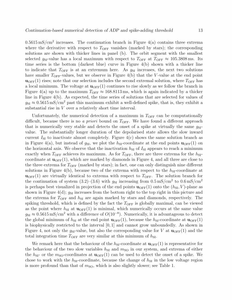
0.5615 mS/cm2 increases. The continuation branch in Figure 4(a) contains three extremawhere the derivative with respect to TOFF vanishes (marked by stars); the correspondingsolutions are shown with thicker lines in panel (b). The orbit segment with the smallestselected gSI-value has a local maximum with respect to TOFF at TOFF ≈ 105.3808 ms. Itstime series is the bottom (darkest blue) curve in Figure 4(b) shown with a thicker lineto indicate that TOFF is at an extremum here. As gSI increases, the next two solutionshave smaller TOFF-values, but we observe in Figure 4(b) that the V -value at the end pointuOFF(1) rises; note that our selection includes the second extremal solution, where TOFF hasa local minimum. The voltage at uOFF(1) continues to rise slowly as we follow the branch inFigure 4(a) up to the maximum TOFF ≈ 168.8113 ms, which is again indicated by a thickerline in Figure 4(b). As expected, the time series of solutions that are selected for values ofgSI ≈ 0.5615 mS/cm2 past this maximum exhibit a well-defined spike, that is, they exhibit asubstantial rise in V over a relatively short time interval.

Unfortunately, the numerical detection of a maximum in TOFF can be computationallydifficult, because there is no a priori bound on TOFF. We have found a different approachthat is numerically very stable and detects the onset of a spike at virtually the same gSI-value. The substantially longer duration of the depolarised state allows the slow inwardcurrent ISI to inactivate almost completely. Figure 4(c) shows the same solution branch asin Figure 4(a), but instead of gSI, we plot the hSI-coordinate at the end points uOFF(1) onthe horizontal axis. We observe that the inactivation hSI of ISI appears to reach a minimumexactly when TOFF achieves its maximum. As for TOFF, there are three extrema for the hSI-coordinate at uOFF(1), which are marked by diamonds in Figure 4, and all three are close tothe three extrema for TOFF (marked by stars); in fact, one can only distinguish nine differentsolutions in Figure 4(b), because two of the extrema with respect to the hSI-coordinate atuOFF(1) are virtually identical to extrema with respect to TOFF. The solution branch forthe continuation of system (3.2)–(3.6) with gSI increasing from 0.5 mS/cm2 to 0.6 mS/cm2

is perhaps best visualized in projection of the end points uOFF(1) onto the (hSI, V )-plane asshown in Figure 4(d); gSI increases from the bottom right to the top right in this picture andthe extrema for TOFF and hSI are again marked by stars and diamonds, respectively. Thespiking threshold, which is defined by the fact the TOFF is globally maximal, can be viewedas the point where hSI at uOFF(1) is minimal, which numerically occurs at the same valuegSI ≈ 0.5615 mS/cm2 with a difference of O(10−8). Numerically, it is advantageous to detectthe global minimum of hSI at the end point uOFF(1), because the hSI-coordinate at uOFF(1)is biophysically restricted to the interval [0, 1] and cannot grow unboundedly. As shown inFigure 4, not only the gSI-value, but also the corresponding value for V at uOFF(1) and thetotal integration time TOFF are very similar at this minimum of hSI.

We remark here that the behaviour of the hSI-coordinate at uOFF(1) is representative forthe behaviour of the two slow variables hSI and mSO in our system, and extrema of eitherthe hSI- or the mSO-coordinates at uOFF(1) can be used to detect the onset of a spike. Wechose to work with the hSI-coordinate, because the change of hSI in the low voltage regionis more profound than that of mSO, which is also slightly slower; see Table 1.

14 J. Nowacki, H.M. Osinga and K.T. Tsaneva-Atanasova

1 4#× 1030

150

TOFF

(a)

0 175t

−50

0

V

(b)

0.0 0.3hSI0

150

TOFF

(c)

1 4#× 1030

150

TOFF

(d)

0 175t

−50

0

V

(e)

0.0 0.3hSI

0

150

TOFF

(f)

Figure 5: Continuation of families with two and three spikes that solve (3.2)–(3.6) as afunction of gSI. Panels (a)–(c) illustrate the branch of two-spike solutions continued pastthe critical threshold at gSI ≈ 0.5697 mS/cm2 and panels (d)–(f) show the branch of three-spike solutions, for which the critical threshold lies at gSI ≈ 0.6183 mS/cm2. Panels (a)and (d) show the solution branches of the gSI-dependent families with TOFF on the verticalaxis and the point number # along the branch (in thousands) on the horizontal axis; timeseries for V of selected orbit segments as marked in these panels are visualized in panels (b)and (e), respectively, coloured from dark- to light-blue as gSI increases (exponentially small).The extremal orbit segments with respect to the TOFF are marked by stars on the solutionbranches and shown with thicker lines in panels (b) and (e). Panels (c) and (f) show TOFF

versus the hSI-coordinate at the end points uOFF(1) on the horizontal axis and illustrate thatthese other two solution types also have the extrema of TOFF located at almost the samepoints where hSI at uOFF(1) is at a local minimum or maximum (marked by a diamonds).The insets highlight the smooth behaviour near the global maximum for TOFF. Comparealso with Figure 4.

For the set-up in Auto, we solve system (3.2)–(3.6) and detect the minimum in hSI atuOFF(1) using an optimization approach. To this end, we introduce a parameter denotedheOFF and add the boundary condition

[0, 0, 0, 0, 1] ∗ uOFF(1)− heOFF = 0 (3.7)

Continuation-based numerical detection of ADP and spike-adding threshold 15

to system (3.2)–(3.6). Here, the vector product [0, 0, 0, 0, 1] ∗ uOFF(1) extracts the hSI-coordinate from uOFF(1). We now allow heOFF to vary freely during the continuation; notethat TOFF also remains a free parameter in this 2PBVP. The advantage of such a setupis that Auto can detect folds with respect to the parameter heOFF; since the boundarycondition (3.7) is only satisfied when heOFF equals the value of the hSI-coordinate at the endpoint of a solution {(uON(t),uOFF(t)) | 0 ≤ t ≤ 1} for system (3.2)–(3.6), this means thatAuto effectively detects the extrema of hSI at the end point uOFF(1).

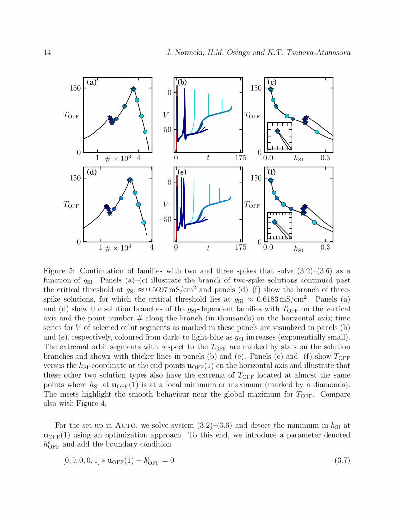
Figure 5 illustrates that our method for detecting the onset of a spike also works forsolutions with more than one spike in their transient response. The next two spike gen-erations occur over exponential small parameter intervals at gSI ≈ 0.5697 mS/cm2 andgSI ≈ 0.6183 mS/cm2; the associated continuations runs are shown in rows 1 and 2 of Fig-ure 5, respectively. The starting solutions for these runs were found as follows. We selectedtwo nearby solutions from the branch computed for Figure 4, namely, at gSI = 0.5690 mS/cm2

and at gSI = 0.6180 mS/cm2. These parameter values are well past the exponentially smallgSI-interval during which the second spike is generated, so that both solutions are orbit seg-ments with one spike followed by the rising part of the next spike up to the (local) maximum.We extended these orbit segments for gSI = 0.5690 mS/cm2 and gSI = 0.6180 mS/cm2 by in-creasing TOFF such that they are solutions of system (3.2)–(3.6) that exhibit two and threespikes, respectively, before ending in a local maximum of the ADP at uOFF(1). Panels (a)and (d) correspond to Figure 4(a) and show the total integration time TOFF versus the pointnumber of the continued branch. The time series in V of selected solutions as marked inpanels (a) and (d) are shown in panels (b) and (e), respectively; the thicker curves indicate asolution for which TOFF achieves a local maximum or minimum, which are marked by starson the continuation branch. Figures 5(c) and (f) show the continuation branch by plottingTOFF versus the hSI-coordinate at the end point uOFF(1), as was done in Figure 4(c) for theone-spike solution branch. This last projection illustrates that extrema of hSI at uOFF(1)(marked by diamonds) appear to be closely related to extrema of TOFF (marked by stars)and the global minimum of hSI at uOFF(1) is a good approximation for the global maximumof TOFF that characterises the onset of the next spike.

4 Computing boundaries between transient bursting

patterns

Our numerical methods for detecting the gSI-values at which the system exhibits the onsetof ADP or the onset of a spike are all based on detecting fold bifurcations for a 2PBVP inAuto (Doedel, 1981; Doedel & Oldeman, 2009). This means that we can subsequently usefold continuation in Auto to trace the onsets of APD or a spike as curves in a two-parameterplane. Such curves would form the boundaries between different bursting behaviours of themodel. We illustrate this by computing the boundary curves in the (gFO, gSI)-plane, becausethe magnitude of gFO influences the amplitude of ADP and, thus, the overall excitabil-

16 J. Nowacki, H.M. Osinga and K.T. Tsaneva-Atanasova

ity (Nowacki et al., 2011).There are two types of curves, namely, onset of ADP and onset of a spike. In order to

compute a curve in the (gFO, gSI)-plane that forms a separatrix between regions with andwithout ADP, we start from a solution of the 2PBVP (3.2)–(3.6) that has a fold with respectto gSI; here, only gSI and TOFF are free parameters. A curve that corresponds to the onsetof a new spike, on the other hand, can be started from a solution of the 2PBVP (3.2)–(3.7),where heOFF, gSI and TOFF are the free parameters. We then include gFO in the list of freeparameters and solve the 2PBVP in Auto with the additional constraint that the systemremains at a fold point with respect to gSI (for onset of ADP) or heOFF (for onset of a newspike); the corresponding extended 2PBVP is generated automatically in Auto.

Figure 6 shows the results of the fold continuation in the (gFO, gSI)-plane. The bifurcationdiagram is shown in panel (a) and examples of responses for parameter values in the differentregions are shown in panels (b)–(m). The solid curves in Figure 6(a) are the fold contin-uation branches. We are only interested in the positive quadrant, gFO, gSI ≥ 0 mS/cm2.Furthermore, the bursting regime is bounded from above by the (dashed green) curve ofHopf bifurcations of the full system (2.1). On the other side of this Hopf curve, any short-current injection drives the system into a continuous (tonic) spiking state due to the presenceof a periodic attractor. For reasons that we explain later, we stop the continuation whengFO reaches the value gFO = 17 mS/cm2 (dashed magenta line). The (solid) green curvecorresponds to the onset of ADP; representative responses on either side of this curve inFigures 6(b) and (c) illustrate the transition from a response with no ADP to one with thedistinctive hump at the end of the spike. The blue curves correspond to onsets of a newspike and the blue-to-cyan colouring indicates the increase in the number of spikes. Wecontinued folds of bursts with one to seven spikes; representative responses from the regionswhere the transient burst has an even number of spikes are shown in Figures 6(d)–(g). Notethat we only show the first curve of onset of ADP, because the continuation of onset of ADPfor solutions that already exhibit more than one spike leads to curves that lie virtually ontop of the branches corresponding to onsets of a new spike. We computed some of theseadditional ADP boundaries, but the other regions of responses with no ADP are so smallthat we decided to ignore the distinction between such regimes altogether. Note that thecurves of onsets of the second and third spike lie very close together. Both curves are com-puted by fold continuation in Auto, but the solutions along these two branches are verydifferent when considered in the full solution space (uON(t),uOFF(t), heOFF, gSI, TOFF, gFO).Hence, our method successfully distinguishes the two curves and establishes each bound-ary accurately; note that such boundary curves are much more difficult to determine usingbrute-force simulations.

Continuation-based numerical detection of ADP and spike-adding threshold 17

8 10 12 14 16 18gFO

0.0

0.2

0.4

0.6

0.8

1.0

1.2

1.4

gSI

(a)

(b)

(c)

(d)

(e)

(f)

(g)(h)

(i)

(j)

(k)

(l)

(m)

−80

−60

−40

−20

0

20

V

(b) (c) (d) (e)

−80

−60

−40

−20

0

20

V

(f) (g) (h) (i)

0 50 100t

−80

−60

−40

−20

0

20

V

(j)

0 50 100t

(k)

0 50 100t

(l)

0 50 100t

(m)

(d)

Figure 6: Regions of different model behaviour in the (gFO, gSI)-plane established by foldcontinuation of system (3.2)–(3.6), or with the additional boundary condition (3.7). Panel (a)shows the bifurcation diagram, with an enlargement of the two-spike burst region in the inset,and panels (b)–(m) responses of system (2.1) for the parameter values as marked by dots inpanel (a). The blue curves are the onsets of a spike, and the colour gets lighter as the numberof spikes increases. The solid green curve corresponds to onset of ADP, the dashed greencurve to Hopf and the dashed red curve to saddle-node bifurcation of the full system (2.1).We stopped the computations at the dashed magenta line and the red dot marks the leftend point of the continuation of onsets of a spike.

18 J. Nowacki, H.M. Osinga and K.T. Tsaneva-Atanasova

The advantage of our approach is that it also successfully continues the different curveswhen they accumulate on each other, as is the case in the direction with gFO decreasing. Infact, all seven computed curves appear to merge on the left and also merge with the (green)boundary of ADP. Again, the fold continuation in Auto views each curve as a distinctfamily in the full solution space (uON(t),uOFF(t), heOFF, gSI, TOFF, gFO) that is well separatedfrom the other burst families, so that the accumulation of curves is numerically not an issue.

The continuation for each of the branches that characterise the onset of a spike stopson the boundary of ADP, approximately at the point marked by a red dot in Figure 6(a).Only the boundary of ADP extends to the gFO-axis. The red dot in Figure 6(a) marks thepoint where the hSI-coordinate at uOFF(1) reaches zero. Indeed, the curves of onsets of aspike are computed by continuation of a minimum heOFF in the hSI-coordinate at uOFF(1)and this minimum heOFF decreases as gFO and/or gSI decrease. Since hSI is constrained byEq. (2.2) to the biological range [0, 1], it is not possible to continue the minimum heOFF pastzero. Note that the onset of ADP takes place for much higher values of hSI at uOFF(1) sothat the continuation of this boundary proceeds until gSI = 0.

As mentioned above, we computed seven curves of onsets of a spike, with the last curvemarking the transition between seven and eight spikes in a burst. As shown in Figure 6(a),these boundary curves accumulate in such a way that a left boundary is formed by consecutivesegments of the boundary curves. We extrapolated this boundary (blue dotted line) up tothe (dashed green) Hopf curve indicating the expected extent of the region with spike-addingbehaviour. For example, the response in Figure 6(h) is for a (gFO, gSI)-pair that lies veryclose, but to the right of this extrapolated boundary. This response is a transient burst withnine spikes, hence, there exists at least one additional curve of onset of a new spike beforereaching the Hopf curve.

To the left of the (extrapolated) boundary of the spiking regime, the response is no longera burst, but exhibits a depolarised plateau with an indistinguishable number of extremelysmall-amplitude spikes; two representative responses chosen far apart from each other areshown in Figures 6(i) and (j). This regime is characterised by a slow passage througha Hopf bifurcation of the fast subsystem; see (Baer, Erneux, & Rinzel, 1989; Izhikevich,2006; Ermentrout & Terman, 2010; Desroches, Guckenheimer, Krauskopf, Kuehn, Osinga,& Wechselberger, 2012) for more details on this process. Note that this behaviour is stilltransient and the solution eventually returns to the resting membrane potential.

The red dashed curve in Figure 6(a) is a curve of saddle-node bifurcations of the fullsystem (2.1); above this curve, an additional pair of equilibria coexist with the restingpotential, but only the resting potential is a stable equilibrium. This curve does not act asa boundary for a particular type of bursting, but the presence of the two equilibria altersthe nature of the spike-adding mechanism and TOFF actually goes to infinity at the criticalthreshold, which is now characterised by a (transiently induced) heteroclinic connection toone of the saddle equilibria; see (Nowacki et al., 2012) for more details. While the spike-adding mechanism changes, the responses of the system on either side of the (red dashed)curve of saddle-node bifurcations inside each of the bursting regions is qualitatively the

Continuation-based numerical detection of ADP and spike-adding threshold 19

same. Our approach for finding the onsets of a spike, where we detect a minimum forthe hSI-coordinate at uOFF(1) instead of a maximum for TOFF, also works for (gFO, gSI)-values above this (dashed red) curve of saddle-node bifurcations, though the solution is acoarser approximation and only the (gFO, gSI)-values of the actual critical threshold are foundaccurately here.

As mentioned above, we decided to stop the computations as soon as we reached gFO =17 mS/cm2. For gFO > 17 mS/cm2 the burst response develops a plateau-like ADP thatcontains a number of small-amplitude oscillations. The response shown in Figure 6(k), forgFO just below 17 mS/cm2, illustrates the formation of the plateau-like ADP and Figures 6(l)and (m) are examples of what the response looks like for gFO > 17 mS/cm2. The natureof the transient response changes in a way that is different from adding a new spike andit is more difficult to define the number of spikes in the burst. Other behaviours mayarise for gSI > 17 mS/cm2 that have not been analysed here. Note that the occurrence ofsmall-amplitude oscillations on top of the ADP can lead to convergence problems in Autoand it is challenging to continue the branches for larger values of gFO). These numericaldifficulties are due to the fact that there now exist several nearby solutions that all satisfyboundary condition (3.6), which requires that the end point uOFF(1) lies at an extremumin V . Indeed, for slightly larger TOFF there exist solutions of the 2PBVP (3.2)–(3.7) thatend at a minimum or maximum in V of either one of these small-amplitude oscillations;these solutions all lie close to each other, even when considering the full solution space(uON(t),uOFF(t), heOFF, gSI, TOFF, gFO). Figure 6(a) gives a good overview of the sensitivityof the bursting behaviour in our model to changes in the parameters gSI and gFO. We find thatchanges in gSI have a much larger effect on the bursting behaviour than changes in gFO. Thismeans that the low-voltage activated slow inward currents have larger impact on excitabilityin our model. We distinguish three large regimes in our region of interest: one-spike responseswith ADP, one-spike responses without ADP, and the combined regions of responses withmultiple spikes. As shown in Figure 6(a), the responses with just one spike and with ADPappear to cover the largest area in the parameter plane. Our simplified model has beenderived based on a more detailed, biophysical model (Nowacki et al., 2011) calibrated usingdata from (Brown & Randall, 2009) and agrees with experimental recordings indicating thatthe response with just one spike followed by an ADP is the most robust (Brown & Randall,2009). In addition, the region with no ADP after the first spike is relatively large, which isin line with the experimental results reported by Brown & Randall (2009); Golomb et al.(2006); and Yaari, Yue, & Su (2007).

5 Discussion

In this paper we presented a continuation-based numerical method for the detection of theonsets of after-depolarisation (ADP) as well as a spike in a transient burst. We defined a two-point boundary value problem (2PBVP) that identifies such onsets as special orbit segmentsthat are determined as fold bifurcations in continuation packages such as Auto (Doedel,

20 J. Nowacki, H.M. Osinga and K.T. Tsaneva-Atanasova

1981; Doedel & Oldeman, 2009). The 2PBVP formulation mirrors the stimulation protocolsused in electrophysiological experimental studies, so that the analysis of our model canbe related directly to the experimental results. We have used a relatively simple model andprotocol to illustrate our approach, but our 2PBVP formulation can be adapted, in principle,to suit onsets of other phenomena in applications involving transient responses generated viadifferent stimulation protocols. The advantage of using a model is that we can analyse thesensitivity of the model to any choice of parameters. In particular, we can make predictionsfor parameters that are hard if not impossible to control using experimental techniques, suchas time constants or membrane capacitance.

For the detection of onset of ADP, we use the formal definition of ADP as a local maxi-mum of the membrane potential V and defined the 2PBVP as a system for which the solu-tions are orbit segments that follow the stimulation protocol and end at the local maximumidentifying the ADP. The disappearance of this local maximum, as a parameter is varied,occurs through an inflection point, where the local maximum merges with the precedinglocal minimum. During the continuation of the 2PBVP, the inflection point is detected asa fold with respect to the parameter. The onset of a spike is more challenging, becausethere is no parameter-independent definition of a spiking threshold. Rather than setting anarbitrary critical threshold for V , we use our findings in (Nowacki et al., 2012) that spikeadding occurs via a canard-like mechanism in models of Hodgkin-Huxley type that exhibitdifferent time scales. This means that the onset of a new spike coincides with a maximumin the time TOFF that it takes the transient response to reach the local maximum of ADP asit relaxes back to the resting potential. In this paper, we argue that the drastic increase inTOFF, which indicates the onset of a new spike, must be accompanied by a decrease in theinactivation hSI of the slow inward current. From a numerical point of view, it is better todetect a minimum in this bounded variable hSI at the end point of the orbit segment thatsolves our 2PBVP and we formulate it such that we can again detect this minimum as a foldpoint on the branch; note that this fold is not with respect to the continuation parameters.

We have shown that the detected onsets of ADP and a spike can be continued in atwo-parameter plane to establish regions of different transient behaviour. Identification ofsuch regions corresponds to a parameter sensitivity analysis of transient bursting patternsfound in this class of models. Our analysis shows that there exists a large area in theparameter plane for which the response exhibits a highly depolarised state; see the responsesin Figures 6(i) and (j). Similar behaviour has been observed experimentally (Golomb et al.,2006) by applying the K+-channel blocker Linopirdine. Such a prolonged depolarised stateis potentially very dangerous for the cell, because the membrane potential is away fromthe resting state. This may lead to excessive influx of Ca2+ that can reach toxic levels.We find that this region is relatively large and directly adjacent to the physiological burstsregime. Our findings indicate that hyper-excitable cells (that fire many spikes) could easilybe driven into such a potentially dangerous state. We note that an increase in gFO couldalso be dangerous, as it decreases excitability and leads to a prominent ADP with smalloscillations; see the responses in Figures 6(l) and (m). Such a prolonged ADP can have a

Continuation-based numerical detection of ADP and spike-adding threshold 21

similar effect on the influx of Ca2+. Hence, this behaviour could possibly be detrimental forthe cell as well.

Acknowledgements

The research for this paper was done while JN was a PhD student at the University of Bristol,supported by grant EP/E032249/1 from the Engineering and Physical Sciences ResearchCouncil (EPSRC). The research of KT-A was supported by EPSRC grant EP/I018638/1and that of HMO by grant UOA0718 of the Royal Society of NZ Marsden Fund.

Bibliography

Andersen, P., Morris, R., Amaral, D., Bliss, T., & O’Keefe, J. (2007). The HippocampusBook. New York: Oxford University Press.

Baer, S.M., Erneux, T., & Rinzel, J. (1989). The slow passage through a Hopf bifurcation:Delay, memory effects, and resonance. SIAM J. Appl. Math., 49(1):55–71.

Brown, J.T., & Randall, A.D. (2009). Activity-dependent depression of the spike after-depolarization generates long-lasting intrinsic plasticity in hippocampal CA3 pyramidalneurons. J. Physiology, 587(6):1265–1281.

Brown, J.T., Chin, J., Leiser, S.C., Pangalos, M.N., & Randall, A.D. (2011). Altered intrinsicneuronal excitability and reduced Na(+) currents in a mouse model of Alzheimer’s disease.Neurobiology of Aging, 32(11):, 2109.e1–2109.e14.

Dankowicz, H., & Schilder, F. (2009). CoCo: General-purpose tools for continuationand bifurcation analysis of dynamical systems ; available via http://sourceforge.net/

projects/cocotools.Dankowicz, H., & Schilder, F. (2011). An extended continuation problem for bifurcation

analysis in the presence of constraints. ASME J. Comp. Nonl. Dyn., 6(3):031003.Desroches,M., Guckenheimer, J., Krauskopf, B., Kuehn, C., Osinga, H.M., & Wechselberger,

M. (2012). Mixed-mode oscillations with multiple time scales. SIAM Review, 54(2):211–288.

Doedel, E.J., & Oldeman, B.E. (2009). with major contributions from Champneys, A.R.,Dercole, F., Fairgrieve, T.F., Kuznetsov, Yu.A., Paffenroth, R.C., Sandstede, B., WangX.J., & Zhang, C.H. AUTO-07p Version 0.7: Continuation and bifurcation software forordinary differential equations. Department of Computer Science, Concordia University,Montreal, Canada; available from http://cmvl.cs.concordia.ca/auto/.

Doedel, E.J. (1981). AUTO: A program for the automatic bifurcation analysis of autonomoussystems. Congressus Numerantium, 30:265–284.

Elburg, R.A.J. van, & Ooyen, A. van (2010). Impact of dendritic size and dendritic topologyon burst firing in pyramidal cells. PLoS computational biology, 6(5):e1000781.

22 J. Nowacki, H.M. Osinga and K.T. Tsaneva-Atanasova

Epsztein, J., Brecht, M., & Lee, A.K. (2011). Intracellular determinants of hippocampalCA1 place and silent cell activity in a novel environment. Neuron, 70(1):109–20.

Ermentrout, G.B., & Terman, D.H. (2010). Mathematical Foundations of Neuroscience. NewYork: Springer-Verlag.

Golomb, D., Yue, C., & Yaari, Y. (2006). Contribution of persistent Na+ current and M-type K+ current to somatic bursting in CA1 pyramidal cells: combined experimental andmodeling study. J. Neurophysiology, 96(4):1912–1926.

Govaerts, W., & Dhooge, A. (2002). Bifurcation, bursting and spike generation in a neuralmodel. Int. J. Bifurcation and Chaos, 12(8):1731–1741.

Guckenheimer, J., Gueron, S., & Harris-Warrick, R.M. (1993). Mapping the dynamics of abursting neuron. Philos Trans R Soc Lond, B, Biol Sci, 341(1298):345–59.

Guckenheimer, J., & Kuehn, C. (2009). Computing slow manifolds of saddle type. SIAM J.Appl. Dyn. Sys., 8(3):854–879.

Guckenheimer, J., Tien, J.H., & Willms, A.R. (2005). Bifurcations in the fast dynamics ofneurons: implications for bursting. In Bursting: The Genesis of Rhythm in the NervousSystem (pp. 89–122). Singapore: World Scientific Publishing.

Harvey, C.D., Collman, F., Dombeck, D.A., & Tank, D.W. (2009). Intracellular dynamicsof hippocampal place cells during virtual navigation. Nature, 461(7266):941–946.

Hodgkin, A.L., & Huxley, A.F. (1952). A quantitive descritpion of membrane current andits application to conduction and excitation in nerve. J. Physiology, 105(117):500–544.

Hunter, J. (2007). Matplotlib: A 2D graphics environment. Computing in Science & Engi-neering, 9(3):90–95.

Izhikevich, E.M. (2000). Neural excitability, spiking and bursting. Int. J. Bifurcation andChaos, 10(6):1171–1266.

Izhikevich, E.M. (2006). Dynamical Systems in Neuroscience: The Geometry of Excitabilityand Bursting. Cambridge, MA: MIT Press.

Keener, J.P., & Sneyd, J. (2008). Mathematical Physiology: Cellular Physiology. New York:Springer-Verlag.

Krahe, R., & Gabbiani, F. (2004). Burst firing in sensory systems. Nature Reviews Neuro-science, 5(1):13–23.

Kuznetsov, Yu.A. (1998). Elements of applied bifurcation theory. New York: Springer-Verlag.Lee, A.K., Manns, I.D., Sakmann, B., & Brecht, M. (2006). Whole-cell recordings in freely

moving rats. Neuron, 51(4):399–407.Llinas, R.R. (1988). The intrinsic electrophysiological properties of mammalian neurons:

insights into central nervous system function. Science, 242(4886):1654–1664.Martinez-Conde, S., Macknik, S.L., & Hubel, D.H. (2002). The function of bursts of spikes

during visual fixation in the awake primate lateral geniculate nucleus and primary visualcortex. Proc. Natl. Acad. of Sciences, 99(21):13920–13925.

McCormick, D.A., & Contreras, D. (2001). On the cellular and network bases of epilepticseizures. Annual Review of Physiology, 63(1):815–46.

Nowacki, J., Osinga, H.M., Brown, J.T., Randall, A.D., & Tsaneva-Atanasova, K.T. (2011).

Continuation-based numerical detection of ADP and spike-adding threshold 23

A unified model of CA1/3 pyramidal cells: An investigation into excitability. Progr.Biophysics and Molecular Biology, 105(1-2):34–48.

Nowacki, J., Osinga, H.M., & Tsaneva-Atanasova, K.T. (2012). Dynamical systems analysisof spike-adding mechanisms in transient bursts. J. Mathematical Neuroscience, 2:7.

Oliphant, T. (2007). Python for scientific computing. Computing in Science & Engineering,9(3):10–20.

Osinga, H.M., & Tsaneva-Atanasova, K.T. (2010). Dynamics of plateau bursting dependingon the location of its equilibrium. J. Neuroendocrinology, 22(12):1301–14.

Rinzel, J. (1985). Bursting oscillations in an excitable membrane model. In Ordinary andPartial Differential Equations, (pp. 304–316). Berlin / Heidelberg: Springer-Verlag.

Rinzel, J. (1987). A formal classification of bursting mechanisms in excitable systems. InInt. Congress of Mathematicians, pp. 1578–1593.

Terman, D.H. (1991). Chaotic spikes arising from a model of bursting in excitable mem-branes. SIAM J. Appl. Math., 51(5):1418–1450.

Terman, D.H. (1992). The transition from bursting to continuous spiking in excitable mem-brane models. J. Nonlinear Science, 2(2):135–182.

Thomas, M.J., Watabe, A.M., Moody, T.D., Makhinson, M., & O’Dell, T.J. (1998). Postsy-naptic complex spike bursting enables the induction of LTP by theta frequency synapticstimulation. J. Neuroscience, 18(18):7118–26.

Tsaneva-Atanasova, K.T., Osinga, H.M., Rieß, T., & Sherman, A. (2010). Full systembifurcation analysis of endocrine bursting models. J. Theoretical Biology, pages 1133–1146.

Tsaneva-Atanasova, K.T., Sherman, A., van Goor, F., & Stojilkovic, S.S. (2007). Mecha-nism of spontaneous and receptor-controlled electrical activity in pituitary somatotrophs:Experiments and theory. J. Neurophysiology, 98(1):131–144.

Yaari, Y., Yue, C., & Su, H. (2007). Recruitment of apical dendritic T-type Ca2+ channelsby backpropagating spikes underlies de novo intrinsic bursting in hippocampal epilepto-genesis. J. Physiology, 580(2):435–450.

Yue, C., Remy, S., Su, H., Beck, H., & Yaari, Y. (2005). Proximal persistent Na+ channelsdrive spike afterdepolarizations and associated bursting in adult ca1 pyramidal cells. J.Neuroscience, 25(42):9704–9720.

Yue, C., and Yaari, Y. (2004). KCNQ/M channels control spike afterdepolarization andburst generation in hippocampal neurons. J. Neuroscience, 24(19):4614–4624.