Continuation Hierarchy and Quantifier Scope Oleg Kiselyov and Chung-chieh Shan 1 [email protected]2 [email protected]Abstract. We present a directly compositional and type-directed anal- ysis of quantifier ambiguity, scope islands, wide-scope indefinites and inverse linking. It is based on Danvy and Filinski’s continuation hier- archy, with deterministic semantic composition rules that are uniquely determined by the formation rules of the overt syntax. We thus obtain a compositional, uniform and parsimonious treatment of quantifiers in subject, object, embedded-NP and embedded-clause positions without resorting to Logical Forms, Cooper storage, type-shifting and other ad hoc mechanisms. To safely combine the continuation hierarchy with quantification, we give a precise logical meaning to often used informal devices such as picking a variable and binding it off. Type inference determines variable names, banishing “unbound traces”. Quantifier ambiguity arises in our analysis solely because quantifier words are polysemous, or come in several strengths. The continuation hierarchy lets us assign strengths to quantifiers, which determines their scope. In- definites and universals differ in their scoping behavior because their lex- ical entries are assigned different strengths. PPs and embedded clauses, like the main clause, delimit the scope of embedded quantifiers. Unlike the main clause, their limit extends only up to a certain hierarchy level, letting higher-level quantifiers escape and take wider scope. This inter- play of strength and islands accounts for the complex quantifier scope phenomena. We present an economical “direct style”, or continuation hierarchy on- demand, in which quantifier-free lexical entries and phrases keep their simple, unlifted types. 1 Introduction The proper treatment of quantification has become a large research area ever since Montague called attention to “the puzzling cases of quantification and reference” back in 1974 [1]. The impressive breadth of the area is evident from two recent surveys [2, 3], which concentrate only on interactions of quantifier phrases among themselves (leaving out, for example, binding of pronouns by quantifiers). The two surveys collect a great amount of empirical data – more and more puzzles. There is also a great number of proposals for a theory to explain the puzzles. And yet even the basic features of the theory remain undecided. In the conclusion of her survey [2] Szabolcsi poses the following three challenges that call for significant new research:
Abstract. We present a directly compositional and type-directed anal-ysis of quantifier ambiguity, scope islands, wide-scope indefinites andinverse linking. It is based on Danvy and Filinski’s continuation hier-archy, with deterministic semantic composition rules that are uniquelydetermined by the formation rules of the overt syntax. We thus obtaina compositional, uniform and parsimonious treatment of quantifiers insubject, object, embedded-NP and embedded-clause positions withoutresorting to Logical Forms, Cooper storage, type-shifting and other adhoc mechanisms.To safely combine the continuation hierarchy with quantification, we givea precise logical meaning to often used informal devices such as pickinga variable and binding it off. Type inference determines variable names,banishing “unbound traces”.Quantifier ambiguity arises in our analysis solely because quantifier wordsare polysemous, or come in several strengths. The continuation hierarchylets us assign strengths to quantifiers, which determines their scope. In-definites and universals differ in their scoping behavior because their lex-ical entries are assigned different strengths. PPs and embedded clauses,like the main clause, delimit the scope of embedded quantifiers. Unlikethe main clause, their limit extends only up to a certain hierarchy level,letting higher-level quantifiers escape and take wider scope. This inter-play of strength and islands accounts for the complex quantifier scopephenomena.We present an economical “direct style”, or continuation hierarchy on-demand, in which quantifier-free lexical entries and phrases keep theirsimple, unlifted types.
1 Introduction
The proper treatment of quantification has become a large research area eversince Montague called attention to “the puzzling cases of quantification andreference” back in 1974 [1]. The impressive breadth of the area is evident fromtwo recent surveys [2, 3], which concentrate only on interactions of quantifierphrases among themselves (leaving out, for example, binding of pronouns byquantifiers). The two surveys collect a great amount of empirical data – more andmore puzzles. There is also a great number of proposals for a theory to explainthe puzzles. And yet even the basic features of the theory remain undecided. Inthe conclusion of her survey [2] Szabolcsi poses the following three challengesthat call for significant new research:
2
1. “develop the tools, logical as well as syntactic, that are necessary to accountfor the whole range of existing readings;”
2. “draw the proper empirical distinction between readings that are actuallyavailable and those that are not;”
3. determine “whether ‘spell-out syntax’ is sufficient for the above two pur-poses” [in other words, if quantifier scope can be determined without resort-ing to Logical Form]
This paper takes on the challenges and develops a logical tool that is ex-pressive to capture empirical data – available and unavailable readings – for arange of quantifier phenomena, from quantifier ambiguity to scope islands, wide-scope indefinites and inverse linking. The “spell-out syntax” proved sufficient:we directly compose meanings that are model-theoretic, not trees. There is quitemore work yet to do. Future work dealing with numeric and downward-entailingquantifiers, plural indefinites, and quantificational binding will hopefully clarifypresently ad hoc parameters such as the number of hierarchy levels.
1.1 What is quantifier scope
“The scope of an operator is the domain within which it has the ability to affectthe interpretation of other expressions” [2, §1.1]. In this paper, we concentrateon how a quantifier affects the interpretation of another quantified phrase. Forexample,
(1) I showed every boy a planet.
has the reading that I showed each boy a possibly different planet. The quantifier‘every’ affected the interpretation of ‘a planet’, which refers to a possibly differentplanet for a different boy. That reading is called linear scope. The sentence hasanother – inverse – reading, whereupon each boy was shown the same planet. Theexample thus exhibits quantifier ambiguity. Although the inverse-scope readingof (1) entails the linear reading (which lead to doubts if inverse readings have tobe accounted for at all [4]), this is not always the case. For example, the linearand inverse readings of
(2) Two of the students attended three of the seminars.
(3) Neither student attended a seminar on rectangular circles.
do not entail each other. Szabolcsi [2] demonstrates solid inverse-scope readingson many more examples. A theory of scope must also explain why no quantifierambiguity arises in examples like
(4) That every boy left upset a teacher.
(5) Someone reported that John saw everyone.
(6) Some professor admires every student and hates the Dean.
and yet other examples with a quantifier within an embedded clause, such as
(7) Everyone reported that [Max and some lady] disappeared.
3
are ambiguous. Szabolcsi argues [2, §3.2] that “different quantifier types havedifferent scope-taking abilities”. The theory should therefore support lexical en-tries for quantifiers that take scope differently and compositionally in relationto each other. The present paper describes such a theory.
1.2 Why continuations
Our theory of quantifier scope is based on continuation semantics, which emerged[5, 6] as a compelling alternative to traditional approaches to quantification –Montague’s proper treatment, Quantifier Raising (QR), type-shifting (surveyedby Barker [5]) – as well as to the Minimalism views (surveyed by Szabolcsi [2];she also extensively discusses QR and its empirical inadequacy). Continuationsemantics is compelling because it can interpret quantificational NPs (QNPs)compositionally in situ, without type-shifting, Cooper storage, or building anystructures like Logical Forms beyond overt syntax. Accordingly, QNPs in sub-ject and other positions are treated the same, QNPs and NPs are treated thesame, and scope taking is semantic. Central to the approach is the hypothesisthat “some linguistic expressions (in particular, QNPs) have denotations thatmanipulate their own continuations” [5, §1]. Although continuation semantics isonly a decade old, its origin can be traced to Montague’s proper treatment: “say-ing that NPs denote generalized quantifiers amounts to saying that NPs denotefunctions on their own continuations” [5, §2.2] (see also [6]). Several continu-ation approaches have been developed since Barker’s [5], using so-called controloperators [6–8] or Lambek-Grishin calculus [9].
1.3 Contributions
Like all continuation approaches, our theory features a compositional, uniformand in-situ analysis of QNPs in object, subject and other positions. Moreover,we address the following open issues.
inverse scope, scope islands and wide-scope indefinites One way to ac-count for these phenomena is to combine control operators with metalinguis-tic quotation [10]. More common – see for example [11] – is using a conti-nuation hierarchy, such as Danvy and Filinski’s (D&F) hierarchy [12], whichhas been thoroughly investigated in the Computer Science theory. The com-mon problem, which has not been addressed in the metalinguistic quotationand the previous D&F hierarchy approaches, is avoiding “unbound traces” –preventing denotations with unbound variables. Barker and Shan’s essen-tially ‘variable-free’ semantics [13] side-steps the unbound traces problemaltogether. However it relies on a different and little investigated hierarchy.The corresponding direct-style (see the next point) is unknown.Our approach is the first to give a rigorous account of inverse scope, scopeislands and wide-scope indefinites using the D&F hierarchy. We rely on typesto prevent unbound traces. We formalize the pervasive intuition that a QNPis represented by a trace (QR), pronoun (Montague) or variable (Cooper
4
storage) that gets bound somehow. We make this intuition precise and giveit logical meaning, banishing unbound traces once and for all.
direct style In Barker’s continuation approach [5], every constituent’s denota-tion explicitly receives its continuation, even though few constituents need tomanipulate these continuations. Combining such continuation-passing-style(CPS) denotations is quite cumbersome, as we see in §2.2. Thus, we wouldlike to avoid CPS denotations for quantifier-free constituents, in particular,for lexical entries other than quantifiers. Direct-style continuation semanticslets us combine continuation-manipulating denotations directly with ordi-nary denotations, simplifying analyses and keeping most lexical entries ‘un-complicated’, which we illustrate in §2.3.We present a version of direct-style for the D&F hierarchy. Unlike otherdirect-style approaches [7, 10], ours uses the ordinary λ-calculus and deno-tational semantics rather than operational semantics and a calculus withcontrol operators. Our treatment of inverse scope relies on the properties ofthe D&F hierarchy extensively, as detailed in §4.
source of quantifier ambiguity It is common to explain quantifier ambiguityby the nondeterminism of semantic composition rules [5, 6]. One syntacticformation operation may correspond to several semantic composition func-tions, or the analysis may include operators like ‘lift’ or ‘wrap’ that may befreely applied to any denotation.In contrast, our semantic composition rules are all deterministic. Althoughwe extensively rely on schematic rules to ease notation and emphasize com-monality, how these schemas are instantiated is determined unambiguouslyby types. Furthermore, our analysis has no optional or freely applicablerules or semantic combinators. Each syntactic formation operation mapsto a unique semantic composition operation, and vice versa: each operationon denotations has a syntactic counterpart. This one-to-one correspondencebetween surface syntax and semantic composition underlies our entire ap-proach – which is thus directly compositional. (See [5, §6] for the discussionof compositionality and how nondeterminism in semantic composition rulesconstitutes a threat.)The source of quantifier ambiguity in our approach is solely in the lexicalentries for the quantifier words rather than in the rules of syntactic forma-tion or semantic composition. Different lexical entries for the same quantifierword have denotations corresponding to different levels of the continuationhierarchy, thus having different strength, or ability to scope over wider con-texts.3
One advantage of our approach is better control over overgeneration: whenonly lexical entries are ambiguous, it is easier to see all available denotationsand hence assure against overgeneration.
3 The different lexical entries for the same quantifier have a regular structure. In fact,all higher-strength quantifier entries are mechanically derived from the entry for thelowest-strength quantifier, as shown in Figures 12 and 13. The number of lexicalentries, that is, the assignment of the levels of strength to a quantifier is determinedfrom empirical data.
5
To summarize: our contribution is a directly compositional analysis of quan-tifier ambiguity, scope islands, inverse linking and wide-scope indefinites in theD&F continuation hierarchy, in direct style, without risking unbound traces,and using deterministic semantic composition rules. We analyze QNP in situand compositionally, relying on no structure beyond the overt syntax. All non-determinism is in the choice of lexical entries for quantifier words. The presen-tation uses the familiar denotational semantics.
1.4 The structure of the paper
The warm-up §2 gradually introduces continuation semantics on a small frag-ment and explains our notation and terminology. §2.3 presents the direct-stylecontinuation semantics as an economical CPS-on-demand. We treat bound vari-ables rigorously in §3, with type annotations to infer variable names and to pre-vent unbound variables in final denotations. §4 presents the continuation hierar-chy and uses it to analyze quantifier ambiguity. The corresponding direct-style,or CPS hierarchy on-demand, is described in §4.2. Scope islands, wide-scopeindefinites and briefly inverse linking are the subject of §5.
For illustrations we use a small fragment of English with context-free syn-tax and extensional semantics, extending and refining the fragment throughoutthe paper. Figure 1 shows the relationship between the fragments, illustratingparallel development in CPS and direct style.
The continuation hierarchy of quantifier scope described in the paper hasbeen implemented. The complete Haskell code is available online at http://
okmij.org/ftp/gengo/QuanCPS.hs. The file implements the fragment of thepaper in the spirit of the Penn Lambda Calculator [14], letting the user writeparse trees and determine their denotations. We have used our semantic calcu-lator for all the examples in the paper.
2 Warm-up: the proper continuation treatment ofquantifiers
In this warm-up section, we recall Barker’s continuation semantics [5] and sum-marize it in our notation. Alongside, we also introduce Barker and Shan’s con-tinuation semantics [7, 15] in direct style, which avoids pervasive type lifting oflexical entries. We use the simplicity of the examples to introduce notation andcalculi to be used in further sections.
2.1 Direct semantics
Like Barker [5], we start with a simple, quantifier-free fragment, with context-freesyntax and extensional semantics. The language of denotations is a plain higher-order language, Figure 2 with the obvious model-theoretical interpretation. Thelanguage has base types e and t and function types, for example (e(et)). We will
Fig. 1. Relationship between the fragments used in the paper
Base types υ ::= e | tTypes σ ::= υ | (σσ)
Constants c ::= ∧ | ∨ | ⇒ | ¬ | john | mary | see | . . .Expressions d ::= c | d � d
Fig. 2. The language D of denotations
7
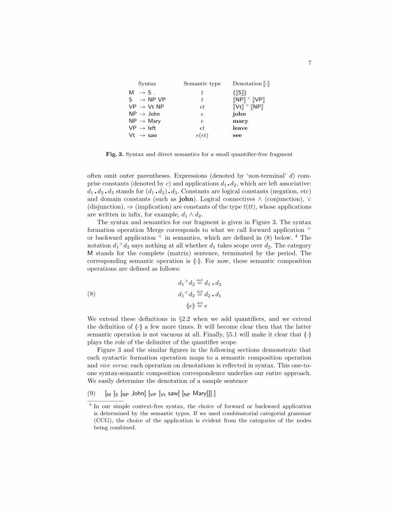
Syntax Semantic type Denotation [[·]]M → S . t (|[[S]]|)S → NP VP t [[NP]] < [[VP]]VP → Vt NP et [[Vt]] > [[NP]]NP → John e johnNP → Mary e maryVP → left et leaveVt → saw e(et) see
Fig. 3. Syntax and direct semantics for a small quantifier-free fragment
often omit outer parentheses. Expressions (denoted by ‘non-terminal’ d) com-prise constants (denoted by c) and applications d1 �d2, which are left associative:d1 � d2 � d3 stands for (d1 � d2) � d3. Constants are logical constants (negation, etc)and domain constants (such as john). Logical connectives ∧ (conjunction), ∨(disjunction),⇒ (implication) are constants of the type t(tt), whose applicationsare written in infix, for example, d1 ∧ d2.
The syntax and semantics for our fragment is given in Figure 3. The syntaxformation operation Merge corresponds to what we call forward application >
or backward application < in semantics, which are defined in (8) below. 4 Thenotation d1
>d2 says nothing at all whether d1 takes scope over d2. The categoryM stands for the complete (matrix) sentence, terminated by the period. Thecorresponding semantic operation is (|·|). For now, these semantic compositionoperations are defined as follows:
(8)
d1>d2
def= d1 � d2
d1<d2
def= d2 � d1
(|e|) def= e
We extend these definitions in §2.2 when we add quantifiers, and we extendthe definition of (|·|) a few more times. It will become clear then that the lattersemantic operation is not vacuous at all. Finally, §5.1 will make it clear that (|·|)plays the role of the delimiter of the quantifier scope.
Figure 3 and the similar figures in the following sections demonstrate thateach syntactic formation operation maps to a semantic composition operationand vice versa: each operation on denotations is reflected in syntax. This one-to-one syntax-semantic composition correspondence underlies our entire approach.We easily determine the denotation of a sample sentence
(9) [M [S [NP John] [VP [Vt saw] [NP Mary]]].]
4 In our simple context-free syntax, the choice of forward or backward applicationis determined by the semantic types. If we used combinatorial categorial grammar(CCG), the choice of the application is evident from the categories of the nodesbeing combined.
8
Types τ ::= σ | τ → τ
Variables x, y, z, v, f, k
Expressions m ::= d | x | λx.m | m m
Reductions m m′ (λx.m)m′ m {x 7→ m′} (β)
Fig. 4. Simply-typed λ-calculus, the language L. (Base types σ and constants d areintroduced in Figure 2.)
to be see �mary � john.
2.2 CPS semantics
We now review continuation semantics, which lets us add quantifiers to ourfragment. Barker [5] has argued that the denotations of quantified phrases needaccess to their context. Here is a simple illustration. Suppose we had a magicdomain constant everyone as the denotation of everyone. We could write themeaning of [M [S John [VP saw [NP everyone]]].] as (|see �everyone � john|), whosemodel-theoretical interpretation must be the same as that of the logical formula∀x. see � x � john. Removing everyone from (|see � everyone � john|) leaves the“term with a hole” (|see � [] � john|) – the context of everyone in the originalterm. We intuit that everyone manages to grab its context, up to the enclosing(|·|), and quantify over it.
To give each term the ability to grab its context, we write the terms ina continuation-passing style (CPS), whereupon each expression receives as anargument its context represented as a function, or continuation. Before we canwrite any CPS term, we have to resolve a small problem. To represent contextswe have to be able to build functions – an operation our language of denotationsD (Figure 2) does not support. Therefore, we “inject” D into the full λ-calculus,with λ-abstractions. This calculus, or language L, is presented in Figure 4.
The expressions of the language D (Figure 2) are all constants of the λ-calculus L; the types of D are all base types of L. In this sense, D is embeddedin L. The language L has its own function types, written with an arrow →.Distinguishing two kinds of function types makes the continuation argumentstand out in CPS terms as well as types. We exploit this distinction in §2.3.
We take → to be right associative and hence we write t → (t → t) ast→ t→ t. Besides the constants, L has variables, abstractions and applications.The application is again left associative, with m1m2m3 standing for (m1m2)m3.L is the full λ-calculus and has reductions, m m′. An expression is in
normal form if no reduction applies to it or any of its sub-expressions. Thenotation m {x 7→ m′} in the β-reduction rule stands for the capture-avoidingsubstitution of m′ for x in m. A unique normal form always exists and can bereached by any sequence of reductions; in other words, L is strongly normalizing.
9
Syntax Semantic type Denotation [[·]]M → S . t (|[[S]]|)S → NP VP (t→ t)→ t [[NP]] < [[VP]]VP → Vt NP ((et)→ t)→ t [[Vt]] > [[NP]]NP → John (e→ t)→ t λk. k johnNP → Mary (e→ t)→ t λk. k maryVP → left ((et)→ t)→ t λk. k leaveVt → saw ((e(et))→ t)→ t λk. k see
NP → everyone (e→ t)→ t λk.∀x. k xNP → someone (e→ t)→ t λk.∃x. k x
Fig. 5. Syntax and continuation semantics for the small fragment
We are set to write CPS denotations for our fragment. Constants like johnhave little to do but to “plug themselves” into their context: λk. k john.5 Here krepresents the context of john within the whole sentence denotation. The wholedenotation must be of the type t; hence k has the type e → t and the type ofthe CPS form of john is (e→ t)→ t. With the CPS denotations, our fragmentnow reads as in Figure 5. The semantic composition operators are now definedas follows.
(10)
m1>m2
def= λk.m1(λf.m2(λx. k(f � x)))
m1<m2
def= λk.m1(λx.m2(λf. k(f � x)))
(|m|) def= m(λv. v)
The CPS form of m1>m2 is λk.m1(λf.m2(λx. k (f � x))): it fills its context k
with f � x, where f is what m1 fills its context with, and x is what m2 fills itscontext with.
Using Figure 5 to compute the denotation of the sample sentence (9) givesus:
= (λk0. (λk. k john)(λx.(λk1. (λk. k see)(λf ′. (λk. k mary)(λx′. k1 (f ′ � x′))))(λf. k0 (f � x))))
(λv. v)
(λk0. (λk. k john)(λx.(λk1. (λk. k mary)(λx′. k1 (see � x′)))(λf. k0 (f � x))))
(λv. v)
5 When a context is represented by a continuation function k, filling the hole in thecontext with a term e – or, plugging e into the context – is represented by theapplication k e.
10
(λk0. (λk. k john)(λx.(λk1. k1 (see �mary))(λf. k0 (f � x))))
(λv. v)
(λk0. (λk. k john)(λx. (k0 ((see �mary) � x))))(λv. v)
(λk0. (k0 ((see �mary) � john)))(λv. v)
((see �mary) � john)
The β-reductions lead to the same expression ((see �mary) � john) as in §2.1.The argument k1 was the continuation of [[saw Mary]]. The term (λk0. . . .) wasthe denotation of the main clause [S John [VP saw Mary]], whose context is empty,represented by λv. v. (If the clause were an embedded one, its context would nothave been empty. We discuss embedded clauses in §5.1.)
Figure 5 contains two extra rows, not present in Figure 3: The CPS semanticslets us express QNPs. The denotation of everyone, λk.∀x. k x, is what we haveinformally argued at the beginning of §2.2 the denotation of everyone should be:the quantifier grabs its continuation k and quantifies over it. The denotation is abit sloppy since we have not yet introduced quantifiers in any of our languages,D or L. Such an informal style, appealing to predicate logic, is very common.For now, we go along; we come back to this point in §3, arguing that it pays tobe formal. Let us see how quantification works:
= (λk0. (λk. k john)(λx.(λk1. (λk. k see)(λf ′. (λk.∀x′′. k x′′)(λx′. k1 (f ′ � x′))))(λf. k0 (f � x))))
(λv. v)
(λk0. (λk1. (λk.∀x′′. k x′′)(λx′. k1 (see � x′))))(λf. k0 (f � john)))
(λv. v)
(λk0. (λk1.∀x′′. k1 (see � x′′))(λf. k0 (f � john)))
(λv. v)
(λk0.∀x′′. k0 (see � x′′) � john)(λv. v)
∀x′′. (see � x′′) � john
The sample sentence “John saw everyone” had the quantifier in the object po-sition, and yet we, unlike Montague, did not have to do anything special toaccommodate it. In fact, comparing (11) against (12) shows that everyone istreated just like Mary. The β-reductions accumulate the context captured by thequantifier until it eventually becomes the full sentence context.
11
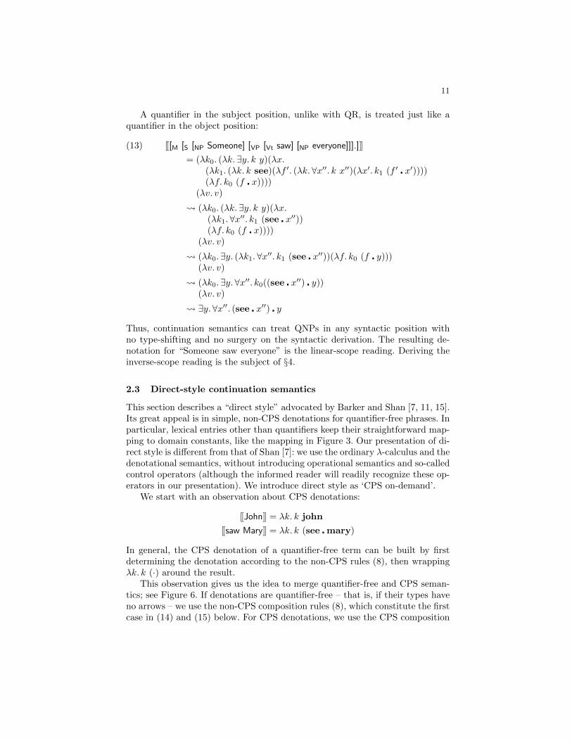
A quantifier in the subject position, unlike with QR, is treated just like aquantifier in the object position:
Thus, continuation semantics can treat QNPs in any syntactic position withno type-shifting and no surgery on the syntactic derivation. The resulting de-notation for “Someone saw everyone” is the linear-scope reading. Deriving theinverse-scope reading is the subject of §4.
2.3 Direct-style continuation semantics
This section describes a “direct style” advocated by Barker and Shan [7, 11, 15].Its great appeal is in simple, non-CPS denotations for quantifier-free phrases. Inparticular, lexical entries other than quantifiers keep their straightforward map-ping to domain constants, like the mapping in Figure 3. Our presentation of di-rect style is different from that of Shan [7]: we use the ordinary λ-calculus and thedenotational semantics, without introducing operational semantics and so-calledcontrol operators (although the informed reader will readily recognize these op-erators in our presentation). We introduce direct style as ‘CPS on-demand’.
We start with an observation about CPS denotations:
[[John]] = λk. k john
[[saw Mary]] = λk. k (see �mary)
In general, the CPS denotation of a quantifier-free term can be built by firstdetermining the denotation according to the non-CPS rules (8), then wrappingλk. k (·) around the result.
This observation gives us the idea to merge quantifier-free and CPS seman-tics; see Figure 6. If denotations are quantifier-free – that is, if their types haveno arrows – we use the non-CPS composition rules (8), which constitute the firstcase in (14) and (15) below. For CPS denotations, we use the CPS composition
12
Syntax Semantic type Denotation [[·]]M → S . t (|[[S]]|)S → NP VP t or (t→ t)→ t [[NP]] < [[VP]]VP → Vt NP et or ((et)→ t)→ t [[Vt]] > [[NP]]NP → John e johnNP → Mary e maryVP → left et leaveVt → saw e(et) see
NP → everyone (e→ t)→ t λk. ∀x.k xNP → someone (e→ t)→ t λk. ∃x.k x
Fig. 6. Syntax and direct-style continuation semantics for the small fragment: themerger of Figures 3 and 5. Lexical entries other than the quantifiers keep the simpledenotations from Figure 3.
rules (10), written as the last case in (14) and (15). When composing CPS andnon-CPS denotations, we implicitly promote the latter into CPS by wrappingthem in λk. k (·). The two middle cases of (14) and (15) show the result of thatpromotion after simplification (β-reductions). Thus the composition rules > and< become schematic with four cases. Likewise, (|·|) becomes schematic with twocases, shown in (16). We stress the absence of any nondeterminism: which ofthe four composition rules to apply is uniquely determined by the types of thedenotations being combined.
m1>m2
def=
m1 �m2 if m1 : (σσ′), m2 :σ
λk.m2(λx. k(m1 � x)) if m1 : (σσ′), m2 : (σ→ t)→ t
Since the sentence [M John [VP saw Mary].] is quantifier-free, its denotation istrivially determined as in §2.1, with no β-reductions – in marked contrast with§2.2. For [M Someone [VP saw Mary].], we compute [[[VP saw Mary]]] as see �mary
13
Levels n, l ∈ NBase types υ ::= e | tTypes σ ::= υ | (σσ)
Annotated types ρ ::= σn
Constants c ::= ∧ | ∨ | ⇒ | ¬ | john | mary | see | . . .Variables n, l
Expressions d ::= c | d � d | n | ∀nd | ∃nd
Type system for judgments d : ρ
n : en+1
d1 : (σ2σ1)n1 d2 : σn22
d1 � d2 : σmax(n1,n2)1
d : tn+1
∀nd : tnd : tn+1
∃nd : tn
Fig. 7. The language DQ of denotations
of the type (et) by the simple rules of (8). The denotation of someone has thetype (e → t) → t, which is a CPS type: it has arrows. The types tell us to usethe third case of (15) to combine [[someone]] with [[[VP saw Mary]]]. We obtainthe final result ∃y. see �mary � y after applying the second case of (16).
Direct style thus keeps quantifier-free lexical entries ‘unlifted’ and removesthe tedium of the CPS semantics. Such CPS-on-demand, or selective CPS, hasbeen used to implement delimited control in Scala [16].
3 The nature of quantification
Before we advance to the main topic, scope and ambiguity, we take a hard lookat logical quantification. So far, we have used quantified logical formulas like∀x. see �x � john without formally introducing quantifiers. The informality, how-ever attractive, makes it hard to specify how to correctly use a logical quantifierto obtain a well-formed closed formula. For example, QR approaches may pro-duce a denotation with an unbound trace, which must then be somehow fixedor avoided. A proper theory should not let sentence denotations with unboundvariables arise in the first place.
We go back to the language D, Figure 2, and extend it with standard first-order quantifiers. The result is the language DQ in Figure 7.
We added variables, which are natural numbers, and two expression forms∀nd and ∃nd to quantify over the variable n. Their model-theoretical semantics isstandard, relying on the variable assignment φ, which maps variables to entities.Then ∀nd is true for the assignment φ iff d is true for every assignment thatdiffers from φ only in the mapping of the variable n.
Figure 7 also extends the type system, with annotated types ρ and judgmentsd : ρ of d having the annotated type ρ. Expression types σ are annotated withthe upper bound on the variable names that may occur in the expression. For
14
m1 : (σ2σ1)n1 m2 : σn22
m1>m2 : σ
max(n1,n2)1
m1 : (σ2σ1)n1 m2 : (σn22 → tl1)→ tl2
m1>m2 : (σ
max(n1,n2)1 → tl1)→ tl2
m1 : ((σ2σ1)n1 → tl1)→ tl2 m2 : σn22
m1>m2 : (σ
max(n1,n2)1 → tl1)→ tl2
m1 : ((σ2σ1)n1 → tl1)→ tl2 m2 : (σn22 → tl3)→ tl1
m1>m2 : (σ
max(n1,n2)1 → tl3)→ tl2
m : t0
(|m|) : t0m : (tn → tn)→ t0
(|m|) : t0
Fig. 8. Typing rules for > in (14) (< is analogous) and for (|·|) in (16).
Fig. 9. Precise denotations of quantifiers and their annotated types. The rest of thefragment remains the same; see Figure 5 or 6.
example, d : σ1 means that d may have (several) occurrences of the variable 0;d : σ2 means d may contain the variables 0 and 1. Our variables are de Bruijnlevels. An expression d of the type σ0 is a closed expression. We will often omitthe type annotation (superscript) 0 – hence D can be regarded as the variable-free fragment of DQ.
The language L will now use the expressions of DQ as constants, and an-notated types ρ as base types. Although the semantic composition functions in(14), (15) and (16) remain the same, their typing becomes more precise, as shownin Figure 8. (Recall (|·|) is the semantic composition function that correspondsto the clause boundary, which we will discuss in detail in §5.1.) As usual, thetyping rules are schematic: m1 and m2 stand for arbitrary expressions of L, σ1and σ2 stand for arbitrary DQ types, and n1, n2, l1, l2, etc. are arbitrary levels.The choice n or l for the name of level metavariables has no significance beyondnotational convenience. The English fragments in Figures 5 and 6 remain prac-tically the same; the quantifier words now receive precisely defined rather thaninformal denotations, and precise semantic types; see Figure 9.
Figure 9 assigns denotations and types to everyone and someone that areschematic in n. That is, there is an instance of the denotation for each naturalnumber n. One may worry about choosing the right n and possible ambiguities.The worries are unfounded. As we demonstrate below, the requirement thatthe whole sentence denotation be closed (that is, have the type t0) uniquelydetermines the choice of n in the denotation schemas for the quantifier words.The choice of variable names n is hence type-directed and deterministic. As anexample, we show the typing derivation for “Someone saw everyone”, which we
The resulting denotation β-reduces to ∃0∀1see �1 �0, as in §2.2. The other deriva-tions in §2.2 and §2.3 are made rigorous similarly.
In the derivation above, the schematic denotation [[someone]] was instantiatedwith n = 0, and the schema [[everyone]] was instantiated with n = 1. It may beunclear how we have made this choice. It is a simple exercise to see that noother choice fits. Relying on the simplicity of the example, we now demonstratethe general method of choosing the variable names n appearing in schematicdenotations. We repeat the derivation, this time assuming that [[someone]] isinstantiated with some variable name n and [[everyone]] is instantiated with somename l. These so-called schematic or logical meta-variables n and l stand forsome natural numbers that we do not know yet. As we build the derivation andfit the denotations, we discover constraints on n and l, which in the end let usdetermine these numbers.
(λk. ∃n(k n))<(see>λk.∀l(k l)) : (tmax (n+1,l+1)→ tl+1)→ tn where n+1 = l
(|(λk. ∃n(k n))<(see>λk.∀l(k l))|) : t0 where n= 0, max (n+1, l+1) = l+1
In the last-but-one step of the derivation, we attempt to type (λk.∃n(k n))<
(see>λk.∀l(k l)) using the rule
m1 : (σn12 → tl1)→ tl2 m2 : ((σ2σ1)n2 → tl3)→ tl1
m1<m2 : (σ
max(n1,n2)1 → tl3)→ tl2
.
This attempt only works if n + 1 = l, because according to the rule, the typesof m1 and m2 must share the same name l1. In the last step of the derivation,applying the typing rule for (|·|) from Figure 8 gives two other constraints: n = 0and max (n+ 1, l + 1) = l + 1. The three constraints have a unique solution:n = 0, l = 1.
More complex sentences with more quantifiers require us to deal with morevariable names n1, n2, n3, etc., and more constraints on them. The overall prin-ciple remains straightforward: since typing is syntax-directed there is never apuzzle as to which typing rule to use at any stage of the derivation. At mostone typing rule applies. An application of a typing rule generally imposes con-straints on the levels. We collect all constraints and solve them at the end (someconstraints can be solved as we go).
Accumulating and solving such constraints is a logic programming problem.Luckily, in modern functional and logic programming languages like Haskell,
16
Twelf or Agda, type checking propagates and solves constraints in a very sim-ilar way. If we write our denotations in, say, Haskell, the Haskell type checkerautomatically determines the names of schematic meta-variables and resolvesschematic denotations and rules. We have indeed used the Haskell interpreterGHCi as such a ‘semantic calculator’, which infers types, builds derivations andinstantiates schemas. Like the Penn Lambda Calculator [14], the Haskell inter-preter also reduces terms. We can enter any syntactic derivation at the inter-preter prompt and see its inferred type and its normal-form denotation.
The choice of variable names, dictated by the requirement that sentencedenotations be closed, in turn describes quantifier scopes, as we shall see next.
4 The inverse-scope problem
If we compute the denotation of [M Someone VP.] by the rules of §2.2, we obtain
No matter what VP is, the existential always scopes over it. Thus, we invariablyget the linear-scope reading for the sentence. Obtaining the inverse-scope readingis the problem. One suggested solution [5, 6] is to introduce nondeterminism intosemantic composition rules. We do not find that approach attractive becauseof over-generation: we may end up with a great number of denotations, notall of which correspond to available readings. Explaining different scope-takingabilities of existentials and universals (see §5) also becomes very difficult.
Our solution to inverse scope is the continuation hierarchy [12]. Like Russiandolls, contexts nest. Plugging a term into a context gives a bigger term, whichcan be plugged into another, wider context, and so on. This hierarchy of contextsis reflected in the continuation hierarchy. Quantifiers gain access not only to theirimmediate context but also to a higher-up context, and may hence quantify overouter contexts. We build the hierarchy from the CPS denotations of §2.2, tobe called CPS1 denotations (with the annotated types of §3). We introduce thecorresponding direct style of the hierarchy in §4.2.
Before we begin, let us quickly skip ahead and peek at the final result, tosee the diffference that the continuation hierarchy makes. Eq. (17) will looksomewhat like
(see Eq. (25) for the complete example). VP will now have a chance to introducea quantifier to scope over ∃y.·.
17
We build the hierarchy by iterating the CPS transformation. An expressionmay be re-written in CPS multiple times. Each re-writing adds another continu-ation representing a higher (outer) context [12]. Let us take an example. A termjohn written in CPS takes the continuation argument representing the term’scontext, and plugs itself into that context: λk. k john. Mechanically applying toit the rules of transforming terms into CPS [12] gives λk1. λk2. (k1 john) k2. ThisCPS2 term receives two continuations and plugs john into the inner one, obtain-ing the CPS1 term k1 john that computes the result to be plugged into the outercontext k2. We may diagram the CPS1 term λk1. k1 john as [k1 . . . [john] . . .],that is, john filling in the hole in a context represented by k1. Likewise we dia-gram the CPS2 term λk1. λk2. (k1 john) k2 as [k2
. . . [k1. . . [john] . . .] . . .]. In the
CPS2 case, if k2 represents the outer context, the application k2 e representsplugging e into that context. If k1 is an inner context, k1 e k2 corresponds toplugging e into it and the result into an outer context k2. We shall see soon thattypes make it clear which context, outer or inner, a continuation represents andwhat needs to be plugged into what.
The CPS2 term λk1. λk2. k1 john k2 is however extensionally equivalent tothe CPS1 term λk. k john we started with. In general, if a term uses its continu-ation ‘trivially’,6 further CPS transformations leave the term intact. Thus, afterquantifier-free lexical entries are converted once into CPS, they can be used asthey are at any level of the CPS hierarchy.
Although the CPS2 term of john is same as the CPS1 term, the types differ.The CPS1 type is (e → tn) → tn, telling us that john receives a context to beplugged with a term of the type e giving a term of the type tn. The CPS2-termreceives another continuation k2, representing the outer context tn → tl1 . Thusthe type of λk1. λk2. k1 john k2 is (e → ((tn → tl1) → tl2)) → ((tn → tl1) →tl2). This type is schematic, written with schematic meta-variables n, l1 and l2standing for some variable names to be determined when building a derivation,as described in §3.
In general, types in the CPS hierarchy have a regular structure and can be de-scribed uniformly. The key observation is recurrence of the pattern (tn → tl1)→tl2 that can be represented by its sequence of annotations n, l1, l2. Therefore, weintroduce the notation
where all ns and ls are schematic meta-variables. Since these sequences canbecome very long, we use Greek letters α, β, γ to each stand for a schematicsequence of variable names. All occurrences of the same Greek letter bearingthe same superscripts and subscripts refer to the same sequence. We will state
6 We say that a term uses its continuation argument k trivially if k is used exactly oncein the term, and each application in the term is the entire body of a λ-abstraction.
18
Syntax Semantic type Denotation [[·]]M → S . t0 (|[[S]]|)S → NP VP (tn → {α})→ {β} [[NP]] < [[VP]]VP → Vt NP ((et)n → {α})→ {β} [[Vt]] > [[NP]]NP → John (e→ {α})→ {α} λk. k johnNP → Mary (e→ {α})→ {α} λk. k maryVP → left ((et)→ {α})→ {α} λk. k leaveVt → saw ((e(et))→ {α})→ {α} λk. k see
Fig. 10. Syntax and the CPS2 semantics for the small fragment. α and β are sequencesof schematic meta-variables of length 3, and γ is a sequence of length 2. See the textfor expressions and types of the semantic composition operators >, < and (|·|)
the length of the sequence separately or leave it implicit in the CPS level un-der discussion. Thus the type of λk. k john for any CPS level has the form(e → {α}) → {α}. Juxtaposed Greek letters and schematic variables signifyconcatenated sequences. For example, (18) is compactly written as follows.
{n} = tn
{nαβ} = (tn → {α})→ {β}(19)
4.1 CPS-hierarchy semantics
The CPS2 semantics for our language fragment is shown in Figure 10. Except forthe quantifiers, the figure looks like the ordinary CPS semantics, Figure 5, withthe wholesale replacement of the type t by {α}. The interesting part is quantifierwords. There are now two sets of them, indexed with 1 and 2: the quantifier wordsbecome polysemous, with two possible denotations. Postulating the polysemy ofquantifiers is similar to generalizing the conjunction schema [17], or assumingthe free indexing in LF.
The quantifiers everyone1 and someone1 are the quantifiers from §2.2, whosedenotations are re-written in CPS. For example, the denotation of everyone fromFigure 9 (which is the precise version of that from Figure 5) is λk.∀n(k n); re-writing it in CPS gives λk1. λk2. k1 n (λv. k2(∀nv)). It plugs the variable n intothe (inner) context k1, then plugs the result into ∀n[] and finally into the outercontext k2. Thus, everyone1 quantifies over the immediate, inner context k1, asin §2.2 above. The continuation arguments to everyone1 are used trivially, so thedenotation can be used as it is not only for CPS2 but also for CPS3 and at higherlevels.
The second set of quantifiers quantify over the outer context, as their de-notation says. For example, λk1. λk2.∀n(k1 n k2) plugs the variable n into the
19
inner context k1, plugs the result into k2 and quantifies over the final result. Theinner and the outer contexts are uniquely determined, as shall see shortly.
The semantic combinators > and < in (10) use their continuation argumenttrivially; therefore, they also work for CPS2 and for all other levels of the hier-archy. We need to give them more general schematic types, extending Figure 8so it works at any level of the hierarchy:
m1 : (σn12 → {α})→ {β} m2 : ((σ2σ1)n2 → {γ})→ {α}
m1<m2 : (σ
max(n1,n2)1 → {γ})→ {β}
(20)
m1 : ((σ2σ1)n1 → {α})→ {β} m2 : (σn22 → {γ})→ {α}
m1>m2 : (σ
max(n1,n2)1 → {γ})→ {β}
(21)
We only need to change (|·|) to account for the two continuation arguments,and hence, two initial continuations:
(22) (|m|) def= m(λv. λk2. k2 v)(λv. v)
The initial CPS1 continuation (λv. λk2. k2 v) plugs its argument into the outercontext; the initial outer context is the empty context. Schematically, (|m|) maybe diagrammed as [k2
[k1m]].
The two sets of quantifiers, level-1 and level-2, treat the inner and outer con-texts differently. The remainder of this subsection presents several examples ofcomputing denotations of sample sentences by using the lexical entries and thecomposition rules of Figure 10 and performing simplifications by β-reductions.As we shall see, the sequence of reductions for, say, Someone1 VP can be dia-grammed at a high level as follows:
[[Someone1 VP.]](23)
= (|[[Someone1 VP]]|)= [k2
[k1[[Someone1 VP]]]]
[k2∃n[k1
n< [[VP]]]]
We hence see that it is the level-1 quantifiers that wedge themselves between theinner context k1 and the outer context k2. We also see that, if the VP containsonly level-1 QNPs, they would quantify over [k1
n< . . .] giving the linear-scopereading. On the other hand, if the VP has a level-2 QNP, it will quantify overthe outer context [k2
∃n[k1n< . . .]] yielding the inverse-scope reading. After this
preview, we describe the computation of denotations in detail.It is a simple exercise to show that [M Someone1 [VP saw everyone1 ].] has
the same linear-scope reading ∃0∀1see � 1 � 0 as computed with the ordinaryCPS, §2.2 – with essentially the same β-reductions shown in that section. Itis also easy to see that [M Someone2 [VP saw everyone2 ].] also has exactly thesame denotation. The interesting cases are the sentences with different levels of
The result still shows the linear-scope reading, because someone2 quantifies overthe wide context and so wins over the narrow-context quantifier everyone1. Onemay wonder how we chose the names of the quantified variables: 0 for someone2and 1 for everyone1. The choice is clear from the final denotation: since it shouldhave the type t0 (that is, be closed), the schema for the corresponding someone2must have been instantiated with n = 0. Therefore, ∀1(see � 1 � 0) must havethe type t1, which determines the schema instantiation for everyone1. One maysay that ‘names follow scope’. The variable names can also be chosen beforeβ-reducing, while building the typing derivation, as demonstrated in §3.
We now make a different choice of lexical entries for the same quantifier wordsin the running example:
(λk2. (λk2.∀0(k2 (see � 0 � 1)))(λv. k2(∃1v)))(λv. v)
(λk2.∀0((λv. k2(∃1v))(see � 0 � 1)))(λv. v)
∀0(∃1(see � 0 � 1))
We obtain the inverse-scope reading: everyone2 quantified over the higher, orwider, context and hence outscoped someone1. This outscoping is noticeable
21
already in the result of the first set of β-reductions, which may be diagrammedas ∀0[k2
∃1[k1see � 0 � [1]]]. Since the universal quantifier eventually got the widest
scope, the schema for everyone2 must have been instantiated with n = 0. Again,the choice of quantifier variable names is determined by quantifiers’ scope.
Thus the continuation hierarchy lets us derive both linear- and inverse-scope readings of ambiguous sentences. The source of the quantifier ambiguityis squarely in the lexical entries for the quantifier words rather than in the rulesof syntactic formation or semantic composition.
4.2 Continuation hierarchy in direct style
Like the ordinary CPS, the CPS hierarchy can also be built on demand. There-fore, we do not have to decide in advance the highest CPS level for our denota-tions, and be forced to rebuild our fragment’s denotations should a new examplecall for yet a higher level. Rather, we build sentence denotations by combiningparts with different CPS levels, or even not in CPS. The primitive parts, lexicalentry denotations, may remain not in CPS (which is the case for all quantifier-free entries) or at the minimum needed CPS level, regardless of the level of otherentries. The incremental construction of hierarchical CPS denotations – buildingup levels only as required – makes our fragment modular and easy to extend.It also relieves us from the tedium of dealing with unnecessarily high-level CPSterms.
Luckily, the semantic combinators < and > capable of combining the denota-tions of different CPS levels have already been defined. They are (14) and (15)in §2.3. The luck comes from the fact that the composition of CPS1 denotationsuses its continuation argument trivially, and therefore, works at any level of theCPS hierarchy. We only need to extend the schema for (|·|), in a regular way:
(26) (|m|) def=
m if m :{0}
m(λv. v) if m :{nn0}
m(λv. λk. kv)(λv. v) if m :{nnl1l1l2l20}
. . .
Applying the schematic definition (26) requires a bit of explanation. If the termm has the type with no arrows, we should compute (|m|) according to the firstcase, which requires m be of the type t0. If m has the type that matches {nn0},that is, (tn → tn)→ t0 for some n, we should use the second case, and so on. Aterm like λk. k (leave � john) of the schematic type {0αα} may seem confusing:its type matches {nn0} (with α instantiated to {0} and n to 0) as well as thetype {nnl1l1l2l20} (with α = {000} and n = l1 = l2 = 0) and all further CPStypes. We can compute (|λk. k (leave � john)|) according to the second or anyfollowing case. The ambiguity is spurious however: whichever of the applicableequations we use, the result is the same – which follows from the fact that a
CPSi term which uses its continuation argument trivially is a CPSi′ term for
22
Syntax Semantic type Denotation [[·]]M → S . t0 (|[[S]]|)S → NP VP tn or (tn → {α})→ {β} [[NP]] < [[VP]]VP → Vt NP etn or ((et)n → {α})→ {β} [[Vt]] > [[NP]]NP → John e johnNP → Mary e maryVP → left et leaveVt → saw e(et) see
Fig. 11. Syntax and the multi-level direct-style continuation semantics for the smallfragment: the merger of Figures 3 and 10. Lexical entries other than the quantifierskeep the simple denotations from Figure 3. Here α, β and γ are sequences of schematicmeta-variables whose length is determined by the CPS level; β is two longer than γ.
all i′ ≥ i [12]. As a practical matter, choosing the lowest-level instance of theschema (26) produces the cleanest derivation.
Figure 11 shows our new fragment.The quantifier-free lexical entries have the simplest denotations and can be
combined with CPSn terms, n ≥ 0. The quantifiers everyone1 and someone1 havethe schematic denotations that can be used at the CPSn level n ≥ 1. The higher-level quantifiers are systematically produced by applying the ↑ combinator of thetype ((en+1 → {α}) → {β}) → ((en+1 → {γα}) → {γβ}) (where α and β havethe same length and γ is one longer).
↑ m def= λk. λk′.m(λv. k v k′)(27)
With the entries in Figure (11), all sample derivations from §4 can be repeatedin direct style with hardly any changes.
Our direct-style multi-level continuation semantics is essentially the same asthat presented in [11]. We do not account for directionality in semantic types(since we use CFG or potentially CCG, rather than type-logical grammars) butwe do account for the levels of quantified variables in types (whereas in [11],quantification was handled informally).
We have thus shown that the CPS hierarchy just as the ordinary CPS can bebuilt on demand, without committing ourselves to any particular hierarchy levelbut raising the level if needed as a denotation is being composed. The result isthe modular semantics, and much simpler and more lucid semantic derivations.From now on, we will use this multi-level direct style.
23
5 Scope islands and quantifier strength
We have used the continuation hierarchy to explain quantifier ambiguity betweenlinear- and inverse-scope readings. We contend that the ambiguity arises becausequantifier words are polysemous: they have multiple denotations correspondingto different levels of the CPS hierarchy. The higher the CPS level, the wider thequantifier scope.
We turn to two further problems. First, just quantifiers’ competing with eachother on their strength (CPS level) does not explain all empirical data. Somesyntactic constructions such as embedded clauses come into play and restrictthe scope of embedded quantifiers. That restriction however does not seem tospread to indefinites: “the varying scope of indefinites is neither an illusion nora semantic epiphenomenon: it needs to be ‘assigned’ in some way” [2]. We shalluse the CPS hierarchy to account for scope islands and to assign the varyingscope to indefinites.
5.1 Scope islands
Like our running example “Someone saw everyone”, two characteristic examples(4) and (5), repeated below, also have two quantifier words.
(28) That every boy left upset a teacher.
(29) Someone reported that John saw everyone.
These examples are not ambiguous however: (28) (the same as (4)) has onlythe inverse-scope reading, whereas (29) (the same as (5)) has only the linear-scope reading. The common explanation (see survey [2]) is that embedded tensedclauses are scope islands, preventing embedded quantifiers from taking scopewider than the island.
To analyze these examples, we at least have to extend our fragment withmore lexical entries and with syntactic forms for clausal NPs, with the corre-sponding semantic combinators.7 Figure 12 shows the additions. Most of themare straightforward. In particular, we generalize quantifying NPs like everyoneto quantifying determiners like every. The determiner receives an extra (et) ar-gument for its restrictor property, of the type of the denotation of a commonnoun.8 Unlike Barker [5], we do not use choice functions in the denotations forthe quantifier determiners. Instead, the denotation of the NP is obtained fromthe denotations of the Det and N by ordinary function application.
Just as quantifying NPs are polysemous, so are quantifying Dets on our anal-ysis: there are weak (or level-1) forms every1 and a1 and strong (or level-2)
7 If the domain of the semantic type t only contains the two truth values, we clearlycannot give an adequate denotation to embedded clauses: the domain is too small.Therefore, we now take the domain of t to be a suitable complete Boolean algebra.
8 This is a simplification: generally speaking, the argument of a Det is not a barecommon noun but a noun modified by PP and other adjuncts. Until we add PP toour fragment in §5.3, the simplification is adequate.
24
Syntax Semantic type Denotation [[·]]VP → Vs that S etn or ((et)n → {α})→ {β} [[Vs]] >(|[[S]]|)NP → that S e That � (|[[S]]|)NP → Det N en or (en → {α})→ {β} [[Det]] [[N]]
N → teacher et teacherN → boy et boyVP → disappeared et disappearVt → upset e(et) upsetVs → report t(et) report
Det → every1 (et)→ (en+1→{(n+1)α})→{nα} λz. λk1. λk2. k1 n (λv.k2 (∀n(z � n⇒ v)))
Det → some1, a1 (et)→ (en+1→{(n+1)α})→{nα} λz. λk1. λk2. k1 n (λv.k2 (∃n(z � n ∧ v)))
Fig. 12. Syntax and the multi-level direct-style continuation semantics for the addi-tional fragment.
forms every2 and a2. Stronger quantifiers outscope weaker ones. For example,[M [S [a1 boy] [upset [every2 teacher]]].] determines the inverse-scope reading∀0(teacher � 0⇒ ∃1(boy � 1 ∧ upset � 0 � 1)).
Recall from Figure 11 how the matrix denotation M→ S. is obtained from thedenotation of the main clause: [[M]] = (|[[S]]|). We see exactly the same pattern forthe clausal NPs in the semantic operations corresponding to Vs that S and that S:in all the cases, the denotation of a clause is enclosed within (|·|), which is thesemantic counterpart of the syntactic clause boundary. The typing rules for (|·|)in Figure 8 specify its result have the type t0, as befits the denotation of a clause.The type t0 is not a CPS type and hence (|[[S]]|) cannot get hold of its context toquantify over. Therefore, if S had any embedded quantifiers, they can quantifyonly as far as the clause. The operation (|·|) thus acts as the scope delimiter,delimiting the context over which quantification is possible. (Incidentally, thesame typing rules of (|·|) severely restrict how this scope-delimiting operationmay be used within lexical entries. For example, (|[[VP]]|) is ill-typed since VPdoes not have the type tn or (tn → {α})→ {β}.)
In case of (28), we obtain the same denotation (30) no matter which lexicalentry we choose for the embedded determiner, every1 (31) or every2 (32). Thequantifier remains trapped in the clause and the sentence is not ambiguous.Incidentally, since all quantifier variables used within a clause will be quantifiedwithin the clause, their names can be chosen regardless of the names of othervariables within the sentence. That’s why the name 0 is reused in (30). Again,names follow scope. A similar analysis applies to (29).
(31) [[[M [NP That [S every1 boy left]] [VP upset [NP a1 teacher]].]]]
25
(32) [[[M [NP That [S every2 boy left]] [VP upset [NP a1 teacher]].]]]
We have demonstrated that a scope island is an effect of the operation (|·|),which is the semantic counterpart of the syntactic clause boundary. In our anal-ysis, each surface syntactic constituent still corresponds to a well-formed deno-tation, and each surface syntactic formation rule still corresponds to a semanticcombinator. Our approach hence is directly compositional.
5.2 Wide-scope indefinites
Given that enclosing all clause denotations in (|·|) traps all quantifiers inside, howdo indefinites manage to get out? And they do get out: “Indefinites acquire theirexistential scope in a manner that does not involve movement and is essentiallysyntactically unconstrained” [2, §3.2.1]. For example:
(33) Everyone reported that [Max and some lady] disappeared.
(34) Most guests will be offended [if we don’t invite some philosopher].
(35) All students believe anything [that many teachers say].
Szabolcsi argued [2] that all these examples are ambiguous. In particular, in (33)(the same as (7)), either different people meant a different lady disappearingalong with Max, or there is one lady that everyone reported as disappearingalong with Max. Interestingly, the example
(36) Someone reported that [Max and every lady] disappeared.
is not ambiguous: there is a single reporter of the disappearance for Max and allladies. The unambiguity of (36) is explained by the embedded clause’s being ascope island, which prevents the universal from taking wide scope. The ambiguityof (33) leads us to conclude that indefinites, in contrast to universals, can scopeout of clauses, complements and coordination structures. Szabolcsi [2] gives alarge amount of evidence for this conclusion. Accordingly, our theory must firstexplain how anything can get out of a scope island, then postulate that onlyindefinites have this escaping ability.
The operation (|·|) that effects the scope island has the schematic type thatcan be informally depicted as CPSi[t]→ CPS0[t] where
CPSi[t] = {α} where the length of α is 2i+1 − 1
Since the result of (|m|) has a CPS0 type, that is t, the result cannot get hold ofany context. Hence we need a less absolutist version of (|·|) which merely lowersrather than collapses the hierarchy. We call that operation (|·|)2, of the informal
schematic type CPS≤2[t] → CPS0[t] and CPSi+2[t] → CPSi[t] where i ≥ 1.Whereas (|m|) delimits all the contexts of m, (|m|)2 delimits only the first twocontexts of the hierarchy. Quantifiers within m of level 3 and higher will be able
26
to get hold of the context of (|m|)2. One may think of (|·|)2 as the inverse of ↑↑.The following example illustrates the lowering:
In (37a) and the identical (37d), the existential quantifies over the potentiallywide context k1. In (37b) and (37c), whose denotations are again identical, ∃0scopes just over leave � 0 and extends no further.
Why did we choose 2 as the number of contexts to delimit at the embeddedclause boundary? Any number i ≥ 2 will work, to explain the quantifier ambi-guity within the embedded clause and wide-scope indefinites. We chose i = 2 fornow pending analysis of more empirical data.
If (37) is the specification for (|·|)2, then (38) below is the implementation. Itis derived from the schema (26) by cutting it off after the third line and insertingthe generic lowering-by-two operation as the final default case.
(38) (|m|)2def=
m if m : {0}
m(λv. v) if m : {nn0}
m(λv. λk. kv)(λv. v) if m : {nnl1l1l2l20}
m(λv. λk. kv)(λv. λk. kv) otherwise
It is easy to show that the definition (38) indeed satisfies (37). A useful lemma isthe identity (↑ m)(λv. λk. kv) = m, easily verified from the definition (27) of ↑.
To make use of this lowering operation (|·|)2, we adjust the lexical entriesin Figure 12 as shown in Figure 13. The main change is replacing (|·|) in thesemantic composition rules for embedded clauses with (|·|)2. In other words, wenow distinguish the main clause boundary from embedded clause boundaries.Figure 13 also reflects our postulate: only indefinites may be at the CPS level 3and higher – not universals.
The typical example (33) can now be analyzed as follows (see Fig. 12 for thedenotations of disappeared and report):
(39) [M Everyone1 reported that [S Max and somei lady disappeared].]
When the level i of somei is 1 or 2, the indefinite is trapped in the scope island.
At the level i = 3, the indefinite scopes out of the clause but is defeated by theuniversal in the subject position, giving us another linear-scope reading, alongthe lines expounded in §2.2.
Syntax Semantic type Denotation [[·]]VP → Vs that S etn or ((et)n → {α})→ {β} [[Vs]] >(|[[S]]|)2NP → that S en or (en → {α})→ {β} That � (|[[S]]|)2NP → NP1 and NP2 en or (en → {α})→ {β} alongWith � [[NP1]] � [[NP2]]N → max e maxN → lady et lady
Fig. 13. Adjustments to the syntax and the multi-level direct-style continuation se-mantics for the additional fragment, to account for wide-scope indefinites. If the sizeof the sequence γ is j, the size of β3 is 3(j + 2) and of β4 is 7(j + 2).
Finally, some4, lowered from level 4 to level 2 as it crosses the embedded clauseboundary, has sufficient strength left to scope over the entire sentence.
Our analysis of inverse linking turns out quite similar to the analysis of wide-scope indefinites. We take the argument NP of a PP to be a scope island, albeitit is evidently a weaker island than an embedded tensed clause. We realize theisland by an operation similar to (|·|)2. Therefore, a strong enough quantifierembedded in NP can escape and take a wide scope. That escaping from theisland corresponds to inverse linking.
To demonstrate our analysis, we extend our fragment with prepositionalphrases; see Figure 14. We add a category of N′ of nouns adjoined with PP.We generalize Det to take as its argument N′ rather than bare common nouns.For simplicity, we use the same (|·|)2 operation for the PP island as we used forthe embedded-clause island. Recall that (∧) is a constant of the type t(tt) andwe write the DQ expression (∧) � d1 � d2 as d1 ∧ d2.
The type of the quantificational determiners shows that a determiner takesa restrictor and a continuation, which may contain n other free variables. Thedeterminer adds a new one, which it then binds. Although the denotations ofdeterminers in Figure 14 bind the variables they themselves introduced, thatproperty is not assured by the type system. For example, nothing prevents usfrom writing ‘bad’ lexical entries like λz.∀nz or 1. Although the type system willensure that the overall denotation is closed, what a binder ends up binding willbe hard to predict. It is an interesting problem to define ‘good’ lexical entries(with respect to scope) and codify the notion in the type system. This is thesubject of ongoing work [18].
28
Syntax Semantic type Denotation [[·]]N′ → N en → nα λx. λk. k ([[N]] � x)N′ → N′ PP en → nα λx. (∧)>([[N′]] x)>([[PP]] x)PP → from NP en → nα λx. (|from> [[NP]] >x|)2NP → Det N′ (en → {α})→ β [[Det]] [[N′]]
λz. λk1. z n (λx. λk2.k1 n (λv. k2 (¬ � ∃n(x ∧ v))))
Fig. 14. Adjustments to the syntax and the multi-level direct-style continuation seman-tics for the additional fragment, to account for prepositional phrases. The higher-levelquantificational determiners are produced with the ↑ operations; see Figure 13 for il-lustration. If the size of the sequence α is j, the size of β is also j and the size of γ is2j + 1.
We analyze inverse linking thusly.
[NP No [N′ [N′ man] [PP from a foreign country]]] was admitted.(41a)
The PP in (41a) contains an ambiguous quantifier. If the quantifier is weak, itis trapped in the PP island and gives the salient reading (41b). If the quantifieris strong enough to escape, the inverse-linking reading (41c) emerges. We thusreproduce quantifier ambiguity for QNP within NP and explain inverse linking.
6 Conclusions
We have given the first rigorous account of linear- and inverse-scope readings,scope islands, wide-scope indefinites and inverse linking based on the D&F con-tinuation hierarchy. Quantifier ambiguity arises because quantifier words arepolysemous, with multiple denotations corresponding to different levels of thehierarchy. The higher the level, the wider the scope. Embedded clauses and PPscreate scope islands by lowering the hierarchy and trapping low-level quantifiers.Higher-level quantifiers (which we postulate only indefinites possess) can escapethe island and take wider scope. The continuation hierarchy lets us assign scopeto indefinites and universals and explain their differing scope-taking abilities.
Our analysis is directly compositional: each surface syntactic constituent cor-responds to a well-formed denotation, and each surface syntactic formation rulecorresponds to a unique semantic combinator.
We have shown how to build the continuation hierarchy modularly and on-demand, without committing ourselves to any particular hierarchy level but
29
raising the level if needed as a denotation is being composed. In particular,quantifier-free lexical entries have unlifted types and simple denotations.
We look forward to extending our analysis to other aspects of scope – howquantifiers interact with coordination (as in (6)), pronouns and polarity items –and to distributivity in universal quantification. We would also like to investigateif hierarchy levels can be correlated with Minimalism features or feature domains.Finally, we plan to extend our analyses of single sentences to discourse.
Acknowledgements We are very grateful to Chris Tancredi for many helpfulsuggestions and a thought-provoking conversation. We thank anonymous review-ers for their comments.
References
[1] Montague, R.: The proper treatment of quantification in ordinary English.In Thomason, R.H., ed.: Formal Philosophy: Selected Papers of RichardMontague. Yale University Press, New Haven (1974) 247–270
[2] Szabolcsi, A.: The syntax of scope. In: Handbook of Contemporary Syn-tactic Theory. Blackwell (2000) 607–634
[3] Szabolcsi, A.: Quantification. Cambridge University Press, Cambridge(2009)
[4] Reinhart, T.: Syntactic domains for semantic rules. In Guenthner, F.,Schmidt, S.J., eds.: Formal Semantics and Pragmatics for Natural Lan-guages. Reidel, Dordrecht (1979) 107–130
[5] Barker, C.: Continuations and the nature of quantification. Natural Lan-guage Semantics 10 (2002) 211–242
[6] de Groote, P.: Type raising, continuations, and classical logic. In van Rooy,R., Stokhof, M., eds.: Proceedings of the 13th Amsterdam Colloquium, In-stitute for Logic, Language and Computation, Universiteit van Amsterdam(2001) 97–101
[7] Shan, C.c.: Linguistic side effects. In Barker, C., Jacobson, P., eds.: DirectCompositionality, New York, Oxford University Press (2007) 132–163
[8] Bekki, D., Asai, K.: Representing covert movements by delimited contin-uations. In: Proceedings of the 6th International Workshop on Logic andEngineering of Natural Language Semantics, Japanese Society of ArtificialIntelligence (2009)
[9] Bernardi, R., Moortgat, M.: Continuation semantics for the Lambek-Grishincalculus. Information and Computation 208 (2010) 397–416
[10] Shan, C.c.: Inverse scope as metalinguistic quotation in operational seman-tics. In Yoshimoto, K., ed.: Proceedings of the 4th International Workshopon Logic and Engineering of Natural Language Semantics, Japanese Societyof Artificial Intelligence (2007) 167–178
[11] Shan, C.c.: Delimited continuations in natural language: Quantificationand polarity sensitivity. In Thielecke, H., ed.: CW’04: Proceedings of the4th ACM SIGPLAN Continuations Workshop. Number CSR-04-1 in Tech.Rep., School of Computer Science, University of Birmingham (2004) 55–64
30
[12] Danvy, O., Filinski, A.: Abstracting control. In: Proceedings of the 1990ACM Conference on Lisp and Functional Programming, New York, ACMPress (1990) 151–160
[14] Champollion, L., Tauberer, J., Romero, M.: The Penn Lambda Calcula-tor: Pedagogical software for natural language semantics. In King, T.H.,Bender, E.M., eds.: Proceedings of the Workshop on Grammar EngineeringAcross Frameworks, Stanford, CA, Center for the Study of Language andInformation (2007) 106–127
[15] Barker, C., Shan, C.c.: Types as graphs: Continuations in type logicalgrammar. Journal of Logic, Language and Information 15 (2006) 331–370
[16] Rompf, T., Maier, I., Odersky, M.: Implementing first-class polymorphicdelimited continuations by a type-directed selective CPS-transform. InHutton, G., Tolmach, A.P., eds.: ICFP ’09: Proceedings of the ACM Inter-national Conference on Functional Programming, New York, ACM Press(2009) 317–328
[17] Partee, B.H., Rooth, M.: Generalized conjunction and type ambiguity. InBauerle, R., Schwarze, C., von Stechow, A., eds.: Meaning, Use and Inter-pretation of Language. Walter de Gruyter, Berlin (1983) 361–383
[18] Kameyama, Y., Kiselyov, O., Shan, C.c.: Combinators for impure yet hy-gienic code generation. In Chin, W.N., Hage, J., eds.: PEPM, New York,ACM Press (2014) 3–14