Continuous-Phase Frequency Shift Keying (FSK) Contents Slide FSK-1 Introduction Slide FSK-2 The FSK Transmitter Slide FSK-3 The FSK Transmitter (cont. 1) Slide FSK-4 The FSK Transmitter (cont. 2) Slide FSK-5 The FSK Transmitter (cont. 3) Slide FSK-6 The FSK Transmitter (cont. 4) Slide FSK-7 The FSK Transmitter (cont. 5) Slide FSK-7 Discrete-Time Implementation Slide FSK-8 Transmitter Implementation (cont.) Slide FSK-9 Switched Oscillator FSK Slide FSK-10 FSK Power Spectral Density Slide FSK-11 FSK Power Spectrum (cont. 1) Slide FSK-12 FSK Power Spectrum (cont. 2) Slide FSK-13 FSK Power Spectrum (cont. 3) Slide FSK-14 Spectrum with Rectangular Pulses Slide FSK-17 Specific Examples of FSK Spectra Slide FSK-18 Spectra for M =2 Slide FSK-19 Spectra for M =4 Slide FSK-20 FSK Demodulation Slide FSK-21 The Frequency Discriminator
Transcript
Continuous-Phase Frequency ShiftKeying (FSK)
Contents
Slide FSK-1 IntroductionSlide FSK-2 The FSK TransmitterSlide FSK-3 The FSK Transmitter (cont. 1)Slide FSK-4 The FSK Transmitter (cont. 2)Slide FSK-5 The FSK Transmitter (cont. 3)Slide FSK-6 The FSK Transmitter (cont. 4)Slide FSK-7 The FSK Transmitter (cont. 5)Slide FSK-7 Discrete-Time ImplementationSlide FSK-8 Transmitter Implementation (cont.)Slide FSK-9 Switched Oscillator FSKSlide FSK-10 FSK Power Spectral DensitySlide FSK-11 FSK Power Spectrum (cont. 1)Slide FSK-12 FSK Power Spectrum (cont. 2)Slide FSK-13 FSK Power Spectrum (cont. 3)Slide FSK-14 Spectrum with Rectangular PulsesSlide FSK-17 Specific Examples of FSK SpectraSlide FSK-18 Spectra for M = 2Slide FSK-19 Spectra for M = 4Slide FSK-20 FSK DemodulationSlide FSK-21 The Frequency Discriminator
Slide FSK-22 Discriminator Block DiagramSlide FSK-24 Example of Discriminator OutputSlide FSK-25 An Approximate DiscriminatorSlide FSK-27 Symbol Clock TrackingSlide FSK-28 Symbol Clock TrackingSlide FSK-30 The Phase-Locked LoopSlide FSK-31 The Phase-Locked Loop (cont. 1)Slide FSK-32 The Phase-Locked Loop (cont. 2)Slide FSK-33 The Phase-Locked Loop (cont. 3)Slide FSK-34 The Phase-Locked Loop (cont. 4)Slide FSK-35 The Phase-Locked Loop (cont. 5)Slide FSK-36 Example of PLL OutputSlide FSK-37 Detection by Tone FiltersSlide FSK-38 Detection by Tone Filters (cont. 1)Slide FSK-39 Computing Ik(N) by IntegrationSlide FSK-40 Computing Ik(N) by FiltersSlide FSK-42 Discrete-Time Tone FiltersSlide FSK-43 Filter Implementation (cont. 1)Slide FSK-44 Discrete-Time Filter Frequency
ResponseSlide FSK-45 Block Diagram of Receiver Using
Tone FiltersSlide FSK-46 Efficient Computation with FIR Tone
FiltersSlide FSK-47 Block Diagram of Receiver Using
Tone Filters
Slide FSK-48 Recursive Implementation of the ToneFilters
Slide FSK-49 Recursive Implementation (cont. 1)Slide FSK-50 Computation for the Recursive
ImplementationSlide FSK-51 Simplification for Binary FSKSlide FSK-52 Simplification for Binary FSK (cont.)Slide FSK-52 Generating a Clock Timing SignalSlide FSK-53 Generating a Clock Signal (cont. 1)Slide FSK-54 Adding a Bandpass Filter to the
Clock TrackerSlide FSK-55 Adding a Bandpass Filter to the
Clock Tracker (cont. 1)Slide FSK-56 Adding a Bandpass Filter to the
Clock Tracker (cont. 2)Slide FSK-57 Detecting the Presence of FSKSlide FSK-58 M = 4 Example of Tone FiltersSlide FSK-59 Segment of FSK SignalSlide FSK-60 3400 Hz Filter Output EnvelopeSlide FSK-61 M = 4 Example (cont.)Slide FSK-62 Preliminary Clock Tracking SignalSlide FSK-63 Bandpass Filtered Clock SignalSlide FSK-64 Superimposed Preliminary and
Bandpass Filtered Clock SignalsSlide FSK-65 Error Probabilities for FSKSlide FSK-66 Orthogonal Signal Sets
Slide FSK-67 Orthogonal Signal Sets (cont. 1)Slide FSK-68 Orthogonal Signal Sets (cont. 2)Slide FSK-69 Orthogonal Signal Sets (cont. 3)Slide FSK-70 Orthogonal Signal Sets (cont. 4)Slide FSK-71 Experiments for FSKSlide FSK-71 EXP 1. Theoretical SpectraSlide FSK-72 EXP 2. Making a TransmitterSlide FSK-72 EXP 2.1 Handshaking SequenceSlide FSK-74 EXP 2.2 Simulating Customer DataSlide FSK-75 EXP 2.3 Measuring the FSK
Power SpectraSlide FSK-76 EXP 3. Making a Receiver Using
an Exact Frequency DiscriminatorSlide FSK-81 EXP 4. Bit-Error Rate TestSlide FSK-83 EXP 5. Making a Receiver Using
an Approximate DiscriminatorSlide FSK-84 EXP 6. Making a Receiver Using
a Phase-Locked LoopSlide FSK-84 EXP 7.1 M = 4 Tone Filter
ReceiverSlide FSK-86 EXP 7.2 Simplified M = 2 Tone
Filter Receiver
Continuous-Phase Frequency
Shift Keying (FSK)
Continuous-phase frequency shift keying (FSK) is
often used to transmit digital data reliably over
wireline and wireless links at low data rates.
Simple receivers with low error probability can be
built. Binary FSK is used in most applications,
often to send important control information.
• Early voice-band telephone line modems used
binary FSK to transmit data at 300 bits per
second or less and were acoustically coupled to
the telephone handset. Teletype machines used
these modems.
• Some HF radio systems use FSK to transmit
digital data at low data rates.
• The 3GPP Cellular Text Telephone Modem
(CTM) for use by the hearing impaired over
regular cellular speech channels uses four level
FSK.
FSK-1
The FSK Transmitter
Converter Carrier fc
.....................
BinaryData
R bits/secD/A
K
symbols/sec(baud rate)
m(t)
M = 2K
Levels
s(t)Serial toParallel
FM
Modulator
fb = R/K
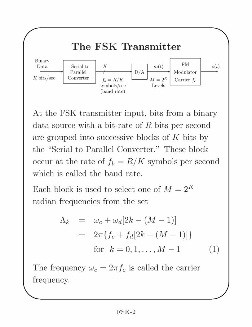
At the FSK transmitter input, bits from a binary
data source with a bit-rate of R bits per second
are grouped into successive blocks of K bits by
the “Serial to Parallel Converter.” These block
occur at the rate of fb = R/K symbols per second
which is called the baud rate.
Each block is used to select one of M = 2K
radian frequencies from the set
Λk = ωc + ωd[2k − (M − 1)]
= 2πfc + fd[2k − (M − 1)]
for k = 0, 1, . . . ,M − 1 (1)
The frequency ωc = 2πfc is called the carrier
frequency.
FSK-2
The FSK Transmitter (cont. 1)
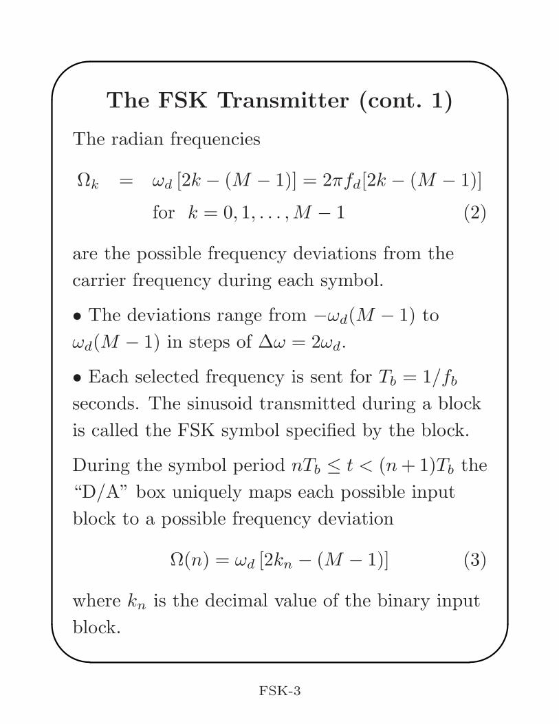
The radian frequencies
Ωk = ωd [2k − (M − 1)] = 2πfd[2k − (M − 1)]
for k = 0, 1, . . . ,M − 1 (2)
are the possible frequency deviations from the
carrier frequency during each symbol.
• The deviations range from −ωd(M − 1) to
ωd(M − 1) in steps of ∆ω = 2ωd.
• Each selected frequency is sent for Tb = 1/fb
seconds. The sinusoid transmitted during a block
is called the FSK symbol specified by the block.
During the symbol period nTb ≤ t < (n+ 1)Tb the
“D/A” box uniquely maps each possible input
block to a possible frequency deviation
Ω(n) = ωd [2kn − (M − 1)] (3)
where kn is the decimal value of the binary input
block.
FSK-3
The FSK Transmitter (cont. 2)
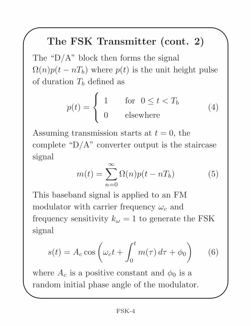
The “D/A” block then forms the signal
Ω(n)p(t− nTb) where p(t) is the unit height pulse
of duration Tb defined as
p(t) =
1 for 0 ≤ t < Tb
0 elsewhere(4)
Assuming transmission starts at t = 0, the
complete “D/A” converter output is the staircase
signal
m(t) =
∞∑
n=0
Ω(n)p(t− nTb) (5)
This baseband signal is applied to an FM
modulator with carrier frequency ωc and
frequency sensitivity kω = 1 to generate the FSK
signal
s(t) = Ac cos
(
ωct+
∫ t
0
m(τ) dτ + φ0
)
(6)
where Ac is a positive constant and φ0 is a
random initial phase angle of the modulator.
FSK-4
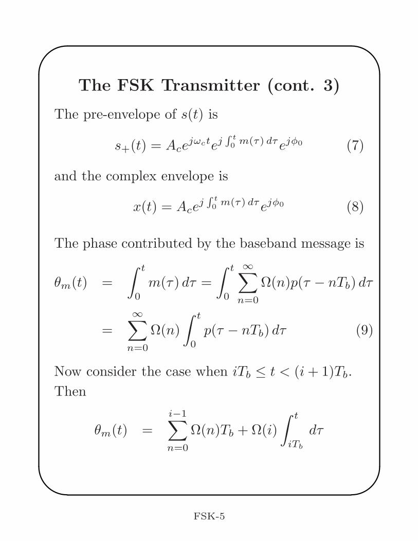
The FSK Transmitter (cont. 3)
The pre-envelope of s(t) is
s+(t) = Acejωctej
∫t
0m(τ) dτejφ0 (7)
and the complex envelope is
x(t) = Acej∫
t
0m(τ) dτejφ0 (8)
The phase contributed by the baseband message is
θm(t) =
∫ t
0
m(τ) dτ =
∫ t
0
∞∑
n=0
Ω(n)p(τ − nTb) dτ
=
∞∑
n=0
Ω(n)
∫ t
0
p(τ − nTb) dτ (9)
Now consider the case when iTb ≤ t < (i+ 1)Tb.
Then
θm(t) =i−1∑
n=0
Ω(n)Tb +Ω(i)
∫ t
iTb
dτ
FSK-5
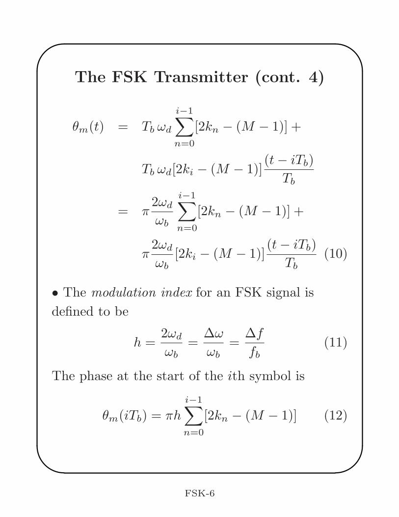
The FSK Transmitter (cont. 4)
θm(t) = Tb ωd
i−1∑
n=0
[2kn − (M − 1)] +
Tb ωd[2ki − (M − 1)](t− iTb)
Tb
= π2ωd
ωb
i−1∑
n=0
[2kn − (M − 1)] +
π2ωd
ωb[2ki − (M − 1)]
(t− iTb)
Tb(10)
• The modulation index for an FSK signal is
defined to be
h =2ωd
ωb=
∆ω
ωb=
∆f
fb(11)
The phase at the start of the ith symbol is
θm(iTb) = πh
i−1∑
n=0
[2kn − (M − 1)] (12)
FSK-6
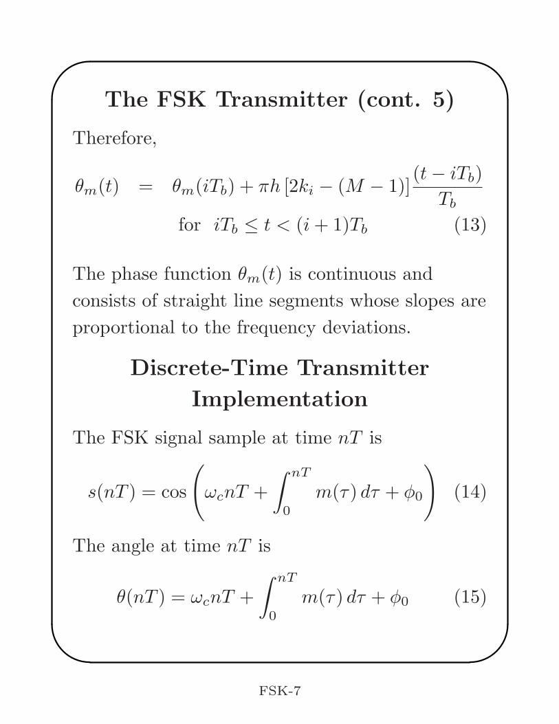
The FSK Transmitter (cont. 5)
Therefore,
θm(t) = θm(iTb) + πh [2ki − (M − 1)](t− iTb)
Tb
for iTb ≤ t < (i+ 1)Tb (13)
The phase function θm(t) is continuous and
consists of straight line segments whose slopes are
proportional to the frequency deviations.
Discrete-Time Transmitter
Implementation
The FSK signal sample at time nT is
s(nT ) = cos
(
ωcnT +
∫ nT
0
m(τ) dτ + φ0
)
(14)
The angle at time nT is
θ(nT ) = ωcnT +
∫ nT
0
m(τ) dτ + φ0 (15)
FSK-7
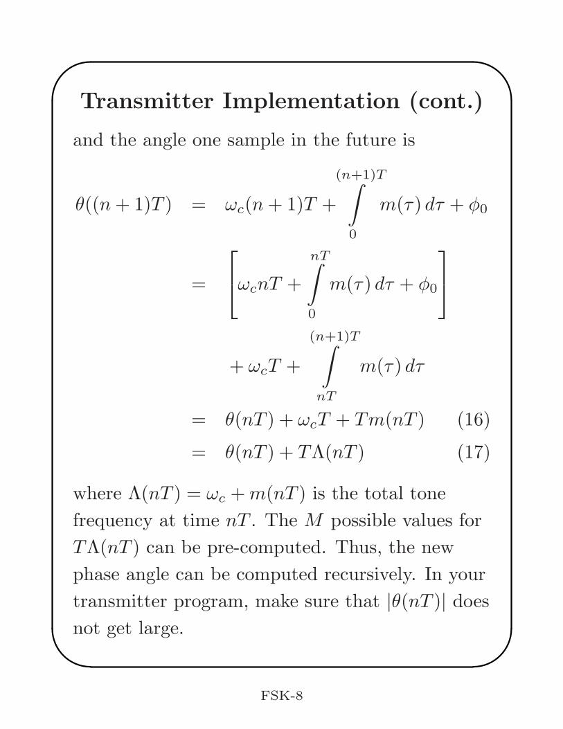
Transmitter Implementation (cont.)
and the angle one sample in the future is
θ((n+ 1)T ) = ωc(n+ 1)T +
(n+1)T∫
0
m(τ) dτ + φ0
=
ωcnT +
nT∫
0
m(τ) dτ + φ0
+ ωcT +
(n+1)T∫
nT
m(τ) dτ
= θ(nT ) + ωcT + Tm(nT ) (16)
= θ(nT ) + TΛ(nT ) (17)
where Λ(nT ) = ωc +m(nT ) is the total tone
frequency at time nT . The M possible values for
TΛ(nT ) can be pre-computed. Thus, the new
phase angle can be computed recursively. In your
transmitter program, make sure that |θ(nT )| does
not get large.
FSK-8
Switched Oscillator FSK
Another approach to FSk would be to switch
between independent tone oscillators. This
switched oscillator approach could cause
discontinuities in the phase function depending on
the tone frequencies and symbol rate. The
discontinuities would cause the resulting FSK
signal to have a wider bandwidth than continuous
phase FSK. It could also cause problems for a
PLL demodulator.
FSK-9
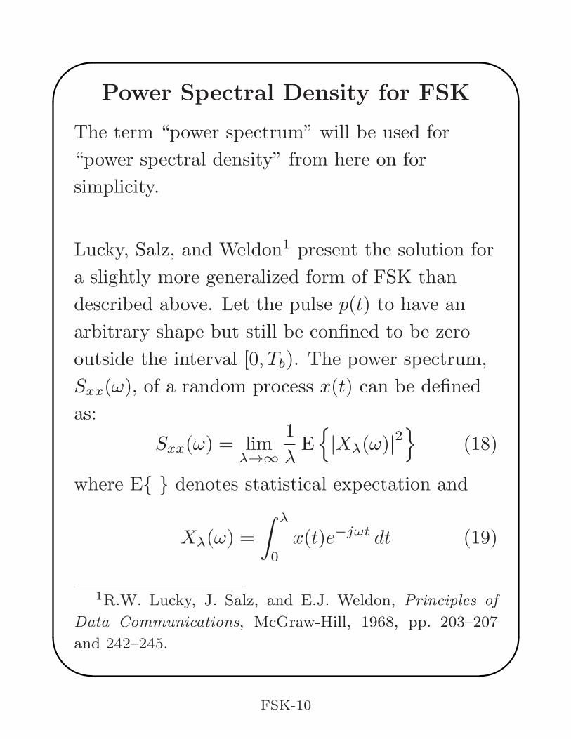
Power Spectral Density for FSK
The term “power spectrum” will be used for
“power spectral density” from here on for
simplicity.
Lucky, Salz, and Weldon1 present the solution for
a slightly more generalized form of FSK than
described above. Let the pulse p(t) to have an
arbitrary shape but still be confined to be zero
outside the interval [0, Tb). The power spectrum,
Sxx(ω), of a random process x(t) can be defined
as:
Sxx(ω) = limλ→∞
1
λE
|Xλ(ω)|2
(18)
where E denotes statistical expectation and
Xλ(ω) =
∫ λ
0
x(t)e−jωt dt (19)
1R.W. Lucky, J. Salz, and E.J. Weldon, Principles of
Data Communications, McGraw-Hill, 1968, pp. 203–207
and 242–245.
FSK-10
Power Spectral Density for FSK
(cont. 1)
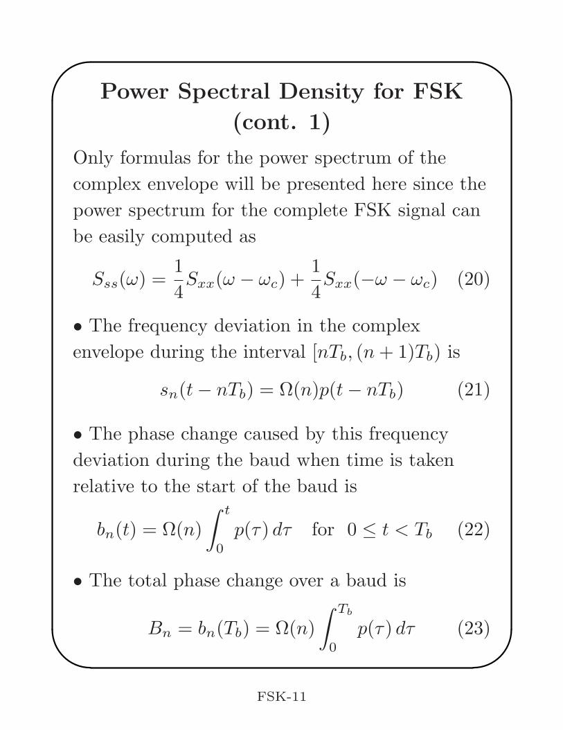
Only formulas for the power spectrum of the
complex envelope will be presented here since the
power spectrum for the complete FSK signal can
be easily computed as
Sss(ω) =1
4Sxx(ω − ωc) +
1
4Sxx(−ω − ωc) (20)
• The frequency deviation in the complex
envelope during the interval [nTb, (n+ 1)Tb) is
sn(t− nTb) = Ω(n)p(t− nTb) (21)
• The phase change caused by this frequency
deviation during the baud when time is taken
relative to the start of the baud is
bn(t) = Ω(n)
∫ t
0
p(τ) dτ for 0 ≤ t < Tb (22)
• The total phase change over a baud is
Bn = bn(Tb) = Ω(n)
∫ Tb
0
p(τ) dτ (23)
FSK-11
Power Spectral Density for FSK
(cont. 2)
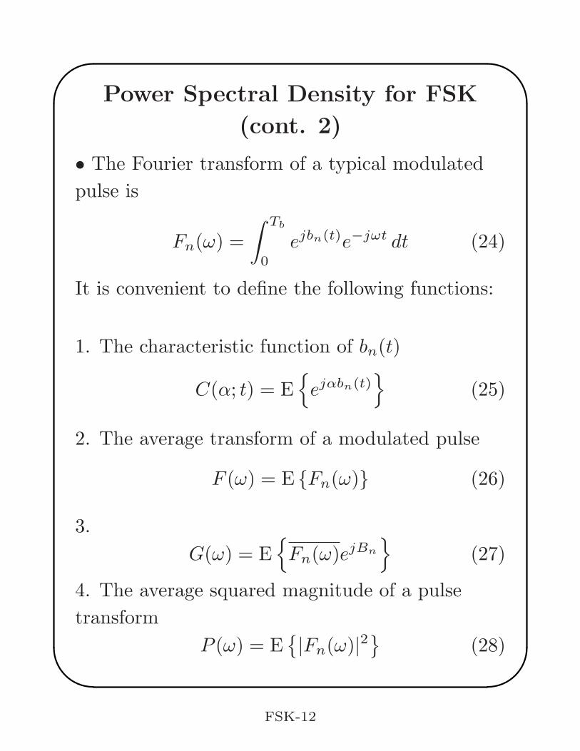
• The Fourier transform of a typical modulated
pulse is
Fn(ω) =
∫ Tb
0
ejbn(t)e−jωt dt (24)
It is convenient to define the following functions:
1. The characteristic function of bn(t)
C(α; t) = E
ejαbn(t)
(25)
2. The average transform of a modulated pulse
F (ω) = E Fn(ω) (26)
3.
G(ω) = E
Fn(ω)ejBn
(27)
4. The average squared magnitude of a pulse
transform
P (ω) = E
|Fn(ω)|2
(28)
FSK-12
Power Spectral Density for FSK
(cont. 3)
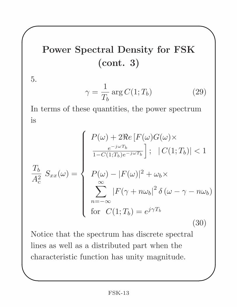
5.
γ =1
TbargC(1;Tb) (29)
In terms of these quantities, the power spectrum
is
Tb
A2c
Sxx(ω) =
P (ω) + 2ℜe [F (ω)G(ω)×
e−jωTb
1−C(1;Tb)e−jωTb
]
; |C(1;Tb)| < 1
P (ω)− |F (ω)|2 + ωb×∞∑
n=−∞
|F (γ + nωb|2δ (ω − γ − nωb)
for C(1;Tb) = ejγTb
(30)
Notice that the spectrum has discrete spectral
lines as well as a distributed part when the
characteristic function has unity magnitude.
FSK-13
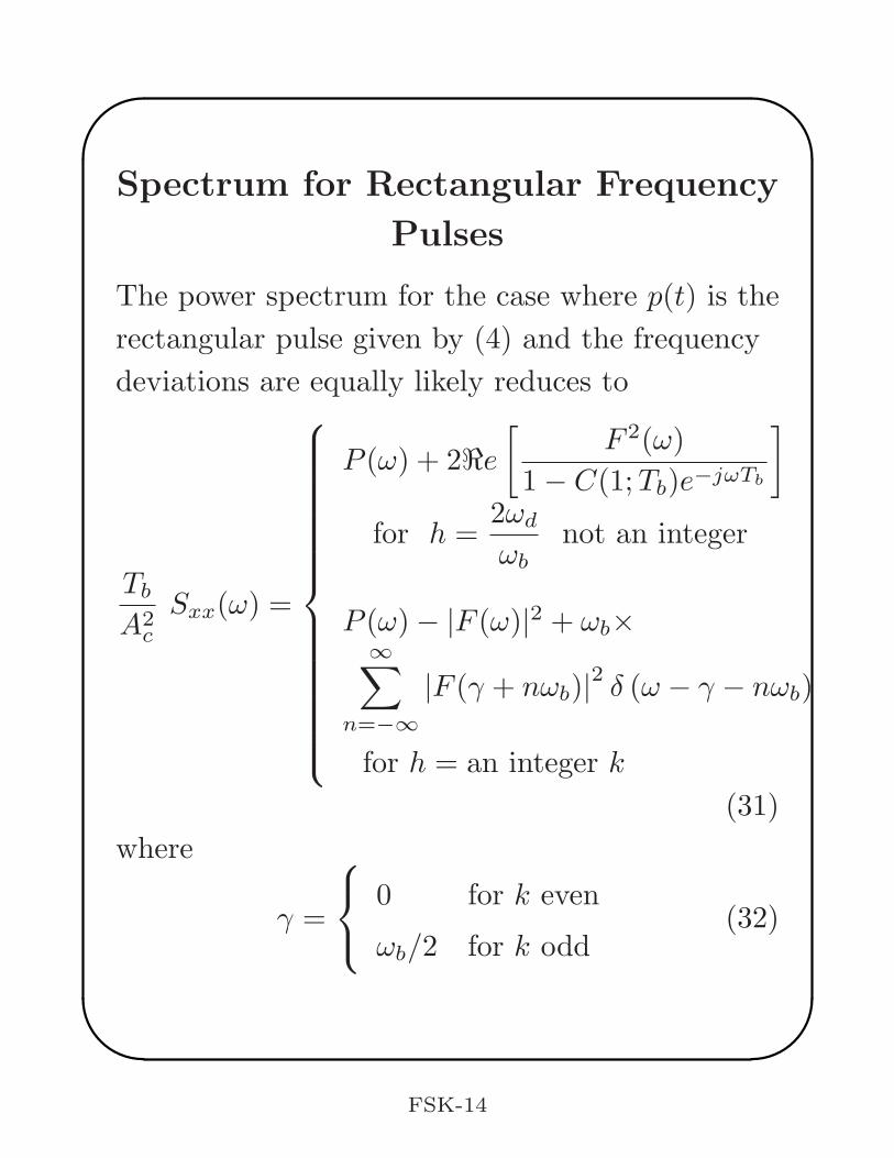
Spectrum for Rectangular Frequency
Pulses
The power spectrum for the case where p(t) is the
rectangular pulse given by (4) and the frequency
deviations are equally likely reduces to
Tb
A2c
Sxx(ω) =
P (ω) + 2ℜe
[
F 2(ω)
1− C(1;Tb)e−jωTb
]
for h =2ωd
ωbnot an integer
P (ω)− |F (ω)|2 + ωb×∞∑
n=−∞
|F (γ + nωb)|2δ (ω − γ − nωb)
for h = an integer k
(31)
where
γ =
0 for k even
ωb/2 for k odd(32)
FSK-14
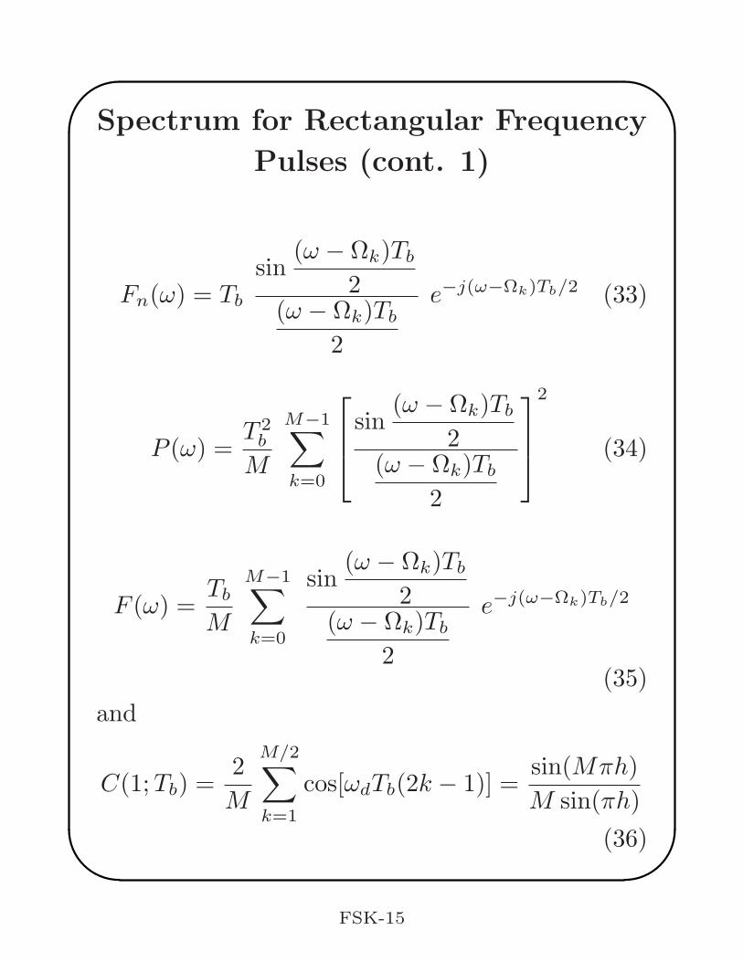
Spectrum for Rectangular Frequency
Pulses (cont. 1)
Fn(ω) = Tb
sin(ω − Ωk)Tb
2(ω − Ωk)Tb
2
e−j(ω−Ωk)Tb/2 (33)
P (ω) =T 2b
M
M−1∑
k=0
sin(ω − Ωk)Tb
2(ω − Ωk)Tb
2
2
(34)
F (ω) =Tb
M
M−1∑
k=0
sin(ω − Ωk)Tb
2(ω − Ωk)Tb
2
e−j(ω−Ωk)Tb/2
(35)
and
C(1;Tb) =2
M
M/2∑
k=1
cos[ωdTb(2k − 1)] =sin(Mπh)
M sin(πh)
(36)
FSK-15
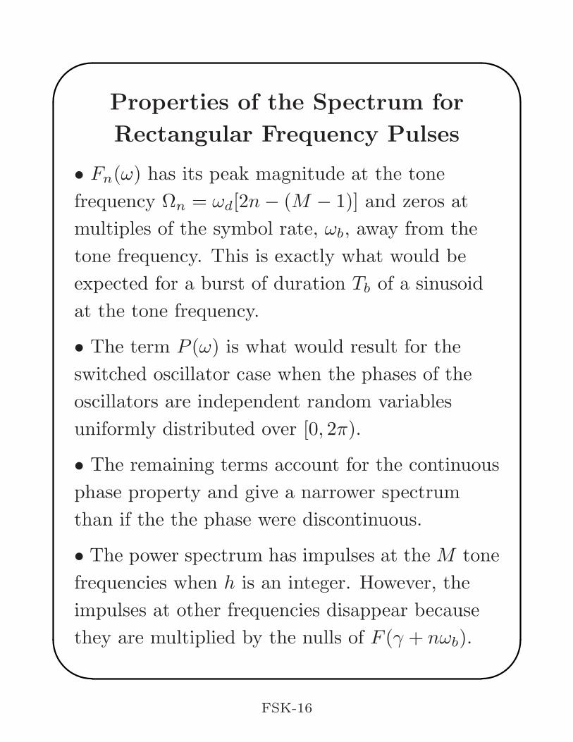
Properties of the Spectrum for
Rectangular Frequency Pulses
• Fn(ω) has its peak magnitude at the tone
frequency Ωn = ωd[2n− (M − 1)] and zeros at
multiples of the symbol rate, ωb, away from the
tone frequency. This is exactly what would be
expected for a burst of duration Tb of a sinusoid
at the tone frequency.
• The term P (ω) is what would result for the
switched oscillator case when the phases of the
oscillators are independent random variables
uniformly distributed over [0, 2π).
• The remaining terms account for the continuous
phase property and give a narrower spectrum
than if the the phase were discontinuous.
• The power spectrum has impulses at the M tone
frequencies when h is an integer. However, the
impulses at other frequencies disappear because
they are multiplied by the nulls of F (γ + nωb).
FSK-16
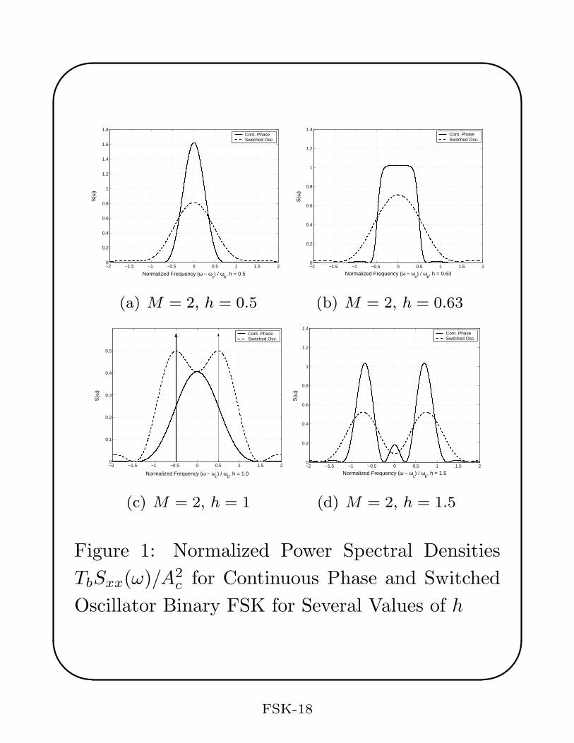
Specific Examples of FSK Spectra
Examples of the power spectral densities for
binary continuous phase and switched oscillator
FSK are shown in Figure 1 for h = 0.5, 0.63, 1 and
1.5. The spectra become more peaked near the
origin for smaller values of h. They become more
and more peaked near −ωd and ωd as h
approaches 1 and include impulses at these
frequencies when h = 1. Bell Labs designed its
Bell 103 binary FSK modem, released in 1962,
with h = 2/3 to avoid impulses in the spectrum
that could cause cross talk in the cables.
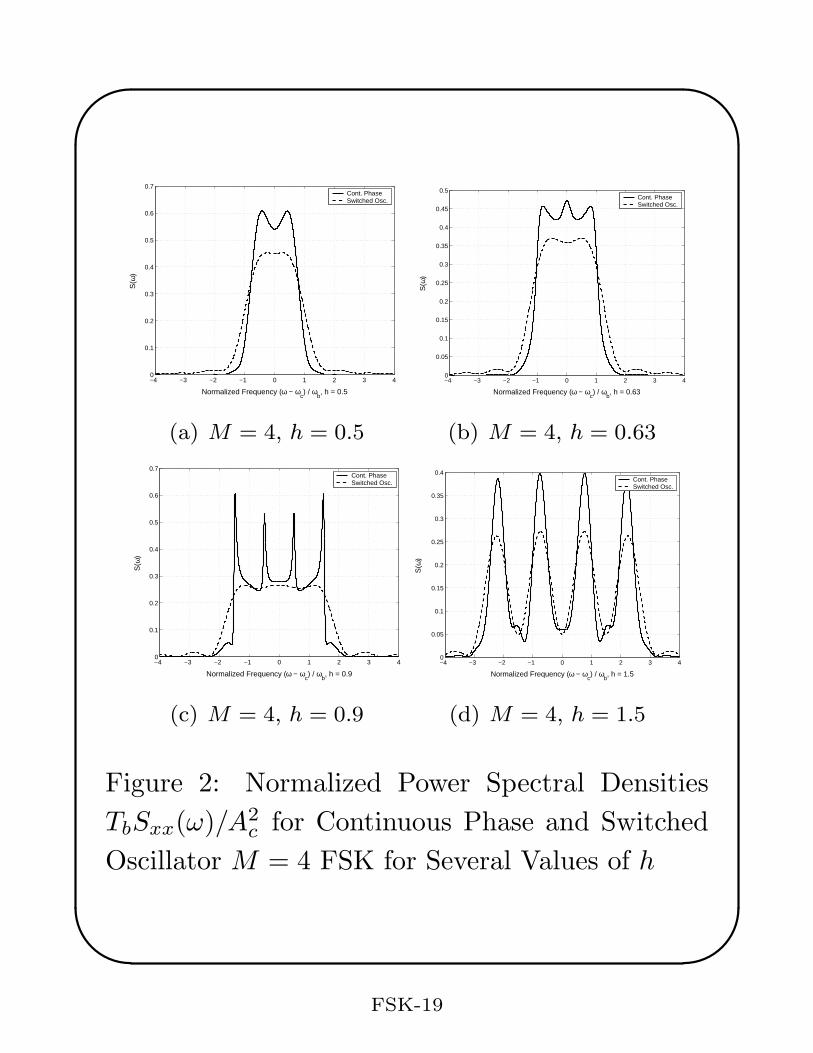
The spectra for M = 4 continuous phase and
switched oscillator FSK are shown in Figure 2 for
h = 0.5, 0.63, 0.9, and 1.5. The CTM with M = 4
uses a symbol rate of 200 baud with a tone
separation of 200 Hz and, thus, has the
modulation index h = 1.
FSK-17
−2 −1.5 −1 −0.5 0 0.5 1 1.5 20
0.2
0.4
0.6
0.8
1
1.2
1.4
1.6
1.8
Normalized Frequency (ω − ωc) / ω
b, h = 0.5
S(ω
)
Cont. PhaseSwitched Osc.
(a) M = 2, h = 0.5
−2 −1.5 −1 −0.5 0 0.5 1 1.5 20
0.2
0.4
0.6
0.8
1
1.2
1.4
Normalized Frequency (ω − ωc) / ω
b, h = 0.63
S(ω
)
Cont. PhaseSwitched Osc.
(b) M = 2, h = 0.63
−2 −1.5 −1 −0.5 0 0.5 1 1.5 20
0.1
0.2
0.3
0.4
0.5
Normalized Frequency (ω − ωc) / ω
b, h = 1.0
S(ω
)
Cont. PhaseSwitched Osc.
(c) M = 2, h = 1
−2 −1.5 −1 −0.5 0 0.5 1 1.5 20
0.2
0.4
0.6
0.8
1
1.2
1.4
Normalized Frequency (ω − ωc) / ω
b, h = 1.5
S(ω
)
Cont. PhaseSwitched Osc.
(d) M = 2, h = 1.5
Figure 1: Normalized Power Spectral Densities
TbSxx(ω)/A2c for Continuous Phase and Switched
Oscillator Binary FSK for Several Values of h
FSK-18
−4 −3 −2 −1 0 1 2 3 40
0.1
0.2
0.3
0.4
0.5
0.6
0.7
Normalized Frequency (ω − ωc) / ω
b, h = 0.5
S(ω
)
Cont. PhaseSwitched Osc.
(a) M = 4, h = 0.5
−4 −3 −2 −1 0 1 2 3 40
0.05
0.1
0.15
0.2
0.25
0.3
0.35
0.4
0.45
0.5
Normalized Frequency (ω − ωc) / ω
b, h = 0.63
S(ω
)
Cont. PhaseSwitched Osc.
(b) M = 4, h = 0.63
−4 −3 −2 −1 0 1 2 3 40
0.1
0.2
0.3
0.4
0.5
0.6
0.7
Normalized Frequency (ω − ωc) / ω
b, h = 0.9
S(ω
)
Cont. PhaseSwitched Osc.
(c) M = 4, h = 0.9
−4 −3 −2 −1 0 1 2 3 40
0.05
0.1
0.15
0.2
0.25
0.3
0.35
0.4
Normalized Frequency (ω − ωc) / ω
b, h = 1.5
S(ω
)
Cont. PhaseSwitched Osc.
(d) M = 4, h = 1.5
Figure 2: Normalized Power Spectral Densities
TbSxx(ω)/A2c for Continuous Phase and Switched
Oscillator M = 4 FSK for Several Values of h
FSK-19
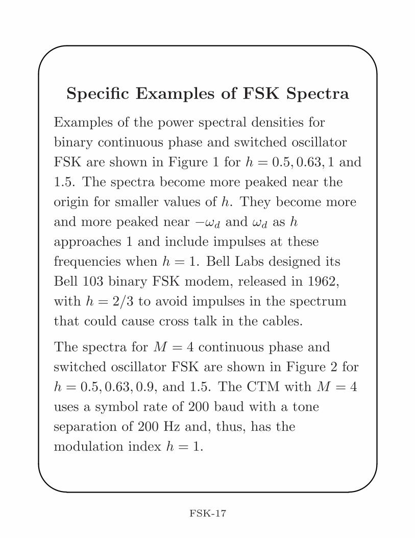
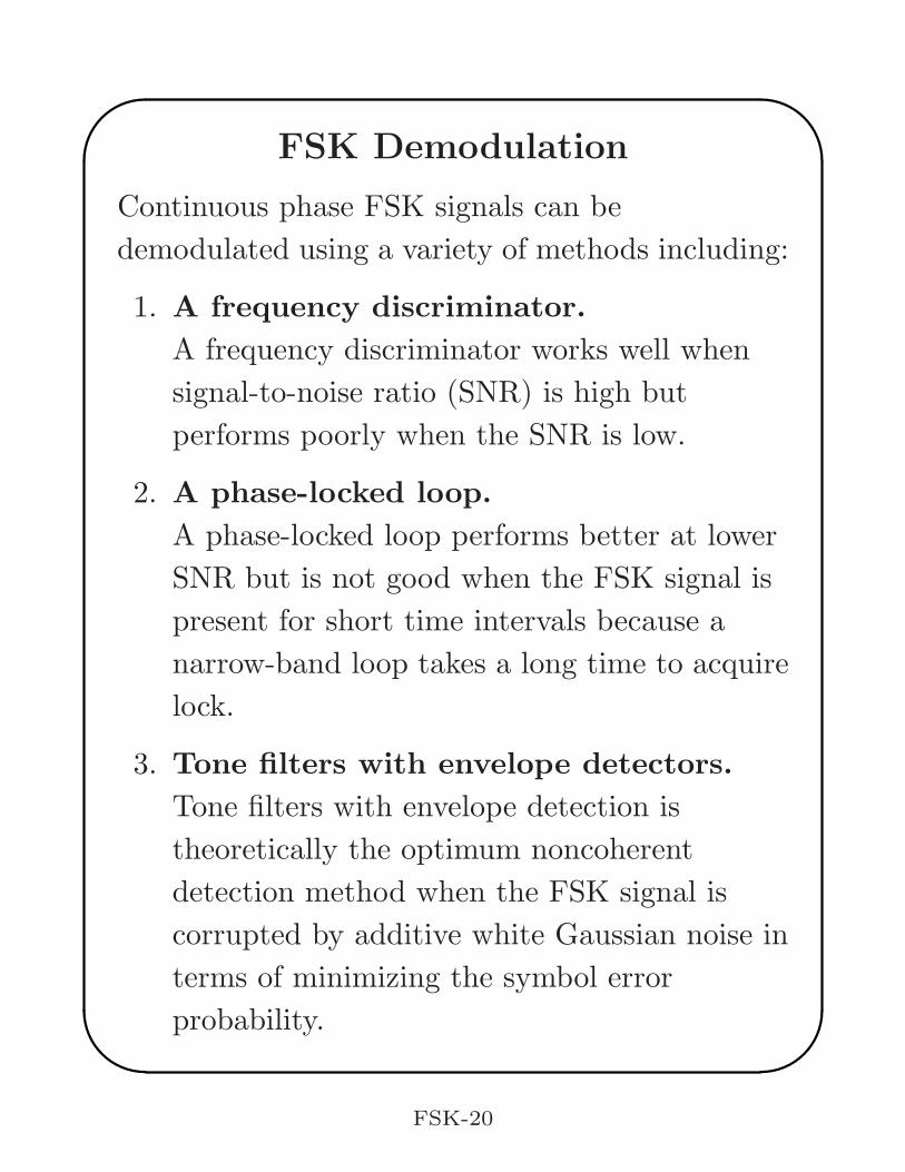
FSK Demodulation
Continuous phase FSK signals can be
demodulated using a variety of methods including:
1. A frequency discriminator.
A frequency discriminator works well when
signal-to-noise ratio (SNR) is high but
performs poorly when the SNR is low.
2. A phase-locked loop.
A phase-locked loop performs better at lower
SNR but is not good when the FSK signal is
present for short time intervals because a
narrow-band loop takes a long time to acquire
lock.
3. Tone filters with envelope detectors.
Tone filters with envelope detection is
theoretically the optimum noncoherent
detection method when the FSK signal is
corrupted by additive white Gaussian noise in
terms of minimizing the symbol error
probability.
FSK-20
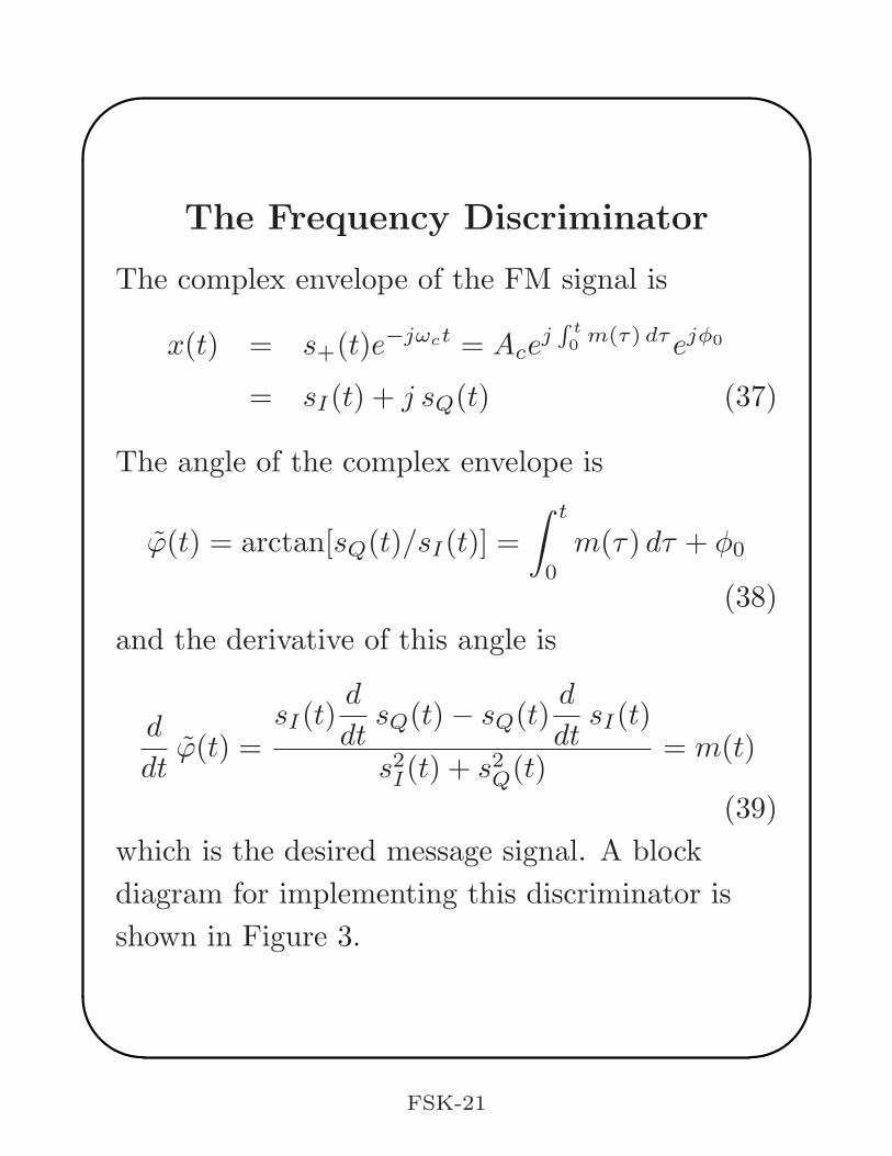
The Frequency Discriminator
The complex envelope of the FM signal is
x(t) = s+(t)e−jωct = Ace
j∫
t
0m(τ) dτejφ0
= sI(t) + j sQ(t) (37)
The angle of the complex envelope is
ϕ(t) = arctan[sQ(t)/sI(t)] =
∫ t
0
m(τ) dτ + φ0
(38)
and the derivative of this angle is
d
dtϕ(t) =
sI(t)d
dtsQ(t)− sQ(t)
d
dtsI(t)
s2I(t) + s2Q(t)= m(t)
(39)
which is the desired message signal. A block
diagram for implementing this discriminator is
shown in Figure 3.
FSK-21
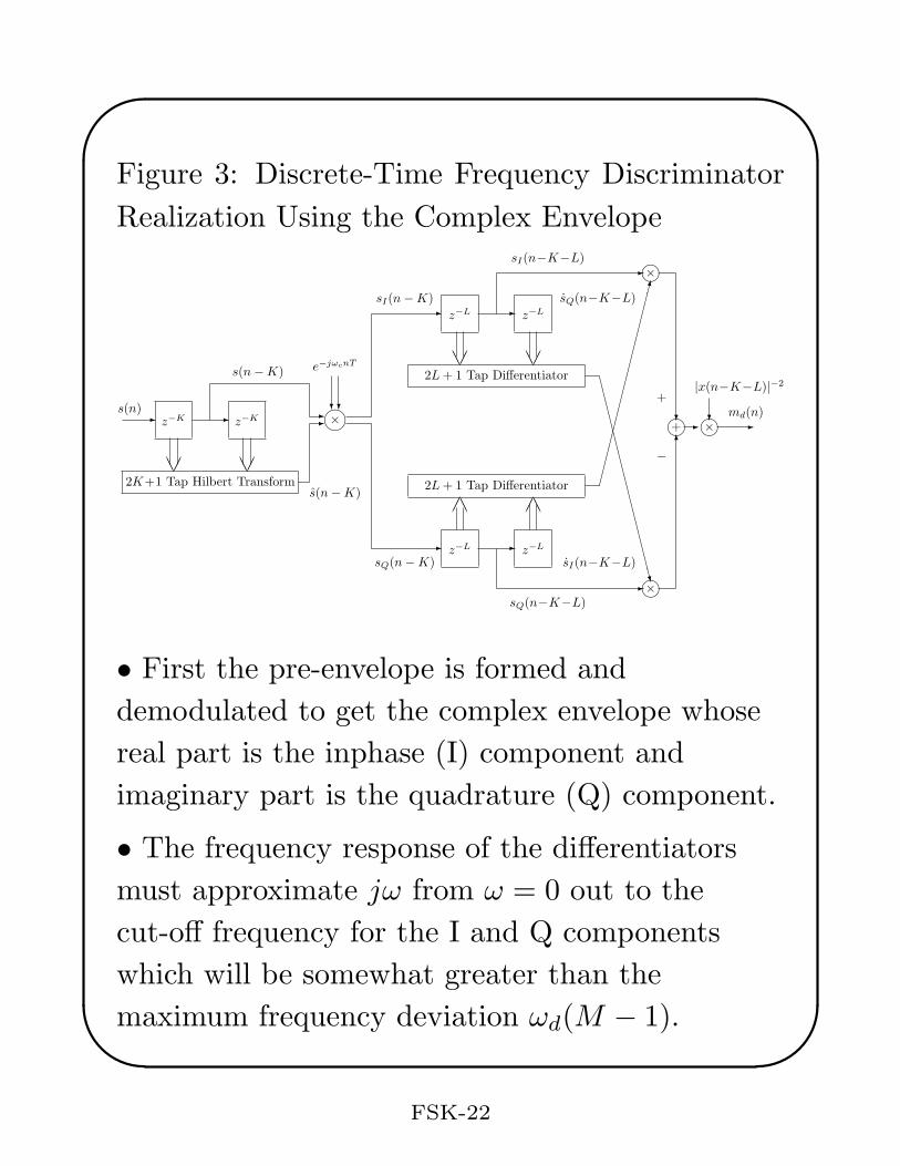
Figure 3: Discrete-Time Frequency Discriminator
Realization Using the Complex Envelope
z−K
z−K
×
2K+1 Tap Hilbert Transform
e−jωcnT
s(n)
s(n − K)
s(n − K)
z−L
z−L
2L + 1 Tap Differentiator
2L + 1 Tap Differentiator
z−L
z−L
sI(n − K)
sQ(n − K)
×
×
❲
+
sI(n−K−L)
sQ(n−K−L)
sQ(n−K−L)
sI(n−K−L)
+
−
×
|x(n−K−L)|−2
md(n)
• First the pre-envelope is formed and
demodulated to get the complex envelope whose
real part is the inphase (I) component and
imaginary part is the quadrature (Q) component.
• The frequency response of the differentiators
must approximate jω from ω = 0 out to the
cut-off frequency for the I and Q components
which will be somewhat greater than the
maximum frequency deviation ωd(M − 1).
FSK-22
Discriminator Implementation
(cont.)
• The differentiator amplitude response should
fall to a small value beyond the cut-off frequency
because differentiation emphasizes high frequency
noise which can cause a significant performance
degradation.
• Notice how the delays through the FIR Hilbert
transform filter and differentiation filters are
matched by taking signals out of the center taps.
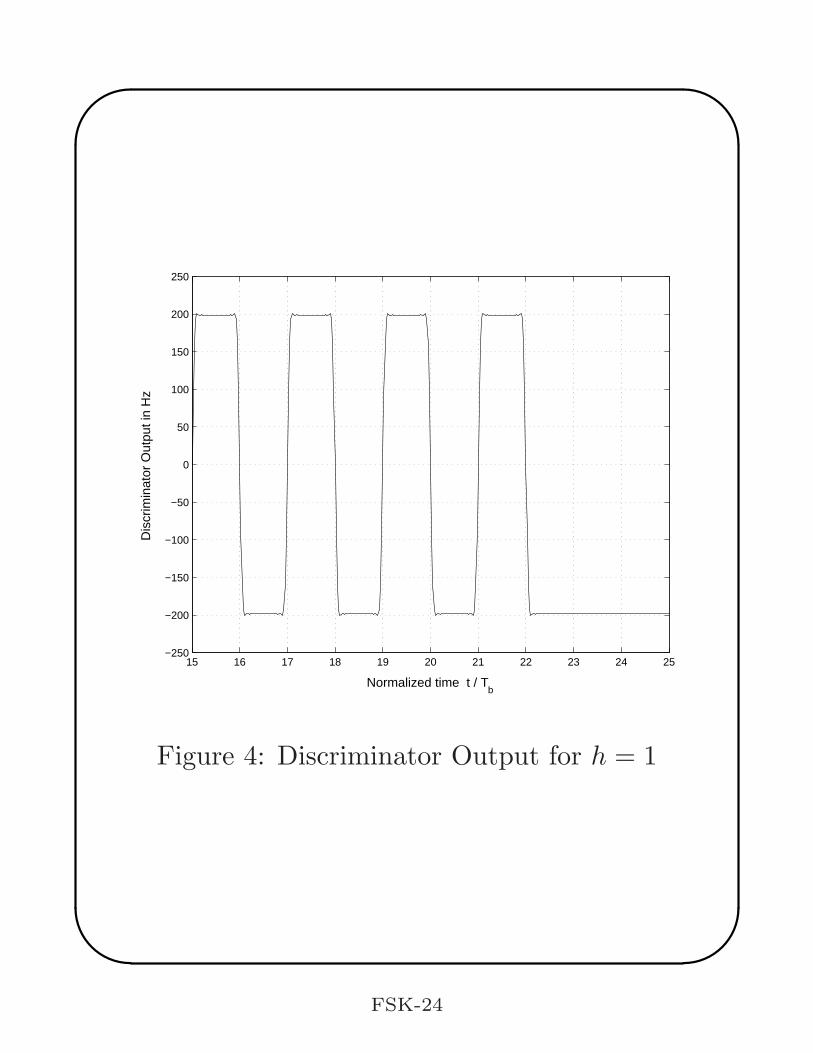
An example of the discriminator output is shown
in Figure 4 when fc = 4000 Hz, fd = 200 Hz, and
fb = 400 Hz, so the modulation index is h = 1.
The tone frequency deviations alternate between
200 and −200 Hz for eight symbols followed by
two symbols with −200 Hz deviation.
FSK-23
15 16 17 18 19 20 21 22 23 24 25−250
−200
−150
−100
−50
0
50
100
150
200
250
Normalized time t / Tb
Dis
crim
inat
or O
utpu
t in
Hz
Figure 4: Discriminator Output for h = 1
FSK-24
A Simple Approximate Frequency
Discriminator
A simpler approximate discriminator will be
derived in this subsection. Let 1/T = fs be the
sampling rate. Usually there will be multiple
samples per symbol so T << Tb. Using the
complex envelope the following product can be
formed:
c(nT ) =1
A2cT
Im
x(nT )x(nT − T )
=1
TIm
ej[∫
nT
0m(τ) dτ+φ0]e−j[
∫nT−T
0m(τ) dτ+φ0]
=1
TIm
ej∫
nT
nT−Tm(τ) dτ
=1
Tsin
∫ nT
nT−T
m(τ) dτ
≈1
Tsin[Tm(nT − T )] =
1
Tsin[m(nT − T )/fs]
≈ m(nT − T )
(40)
To get the final result, the approximation
sinx ≃ x for |x| << 1 was used.
FSK-25
Approximate Discriminator (cont.)
In terms of the inphase and quadrature
components
c(nT ) =1
A2cT
[sQ(nT )sI(nT − T )− sI(nT )sQ(nT − T )]
(41)
and this is the discriminator equation that would
be implemented in a DSP.
As another approach, suppose the derivatives in
(39) are approximated at time nT by
d
dtsI(t)|t=nT ≃
sI(nT )− sI(nT − T )
T(42)
and
d
dtsQ(t)|t=nT ≃
sQ(nT )− sQ(nT − T )
T(43)
Subsituting these approximate derivatives into
(39) gives ddt ϕ(t)|t=nT ≃ c(nT ) exactly as in the
previous approach.
FSK-26
Symbol Clock Acquisition and
Tracking
The discriminator output will look like an
M -level PAM signal with rapid changes at the
symbol boundaries where the frequency deviation
has changed. The discriminator output must be
sampled once per symbol at the correct time to
estimate the transmitted frequency deviation and,
hence, the input data bit sequence.
When the signal-to-noise ratio is large at the
receiver, the sharp transitions in the discriminator
output can be detected.
• A method for doing this is to form the absolute
value of the derivative of the discriminator
output. This will generate a positive pulse
whenever the output level changes.
• A pulse location can be determined by looking
for a positive threshold crossing.
FSK-27
Symbol Clock Acquisition (cont. 1)
• Then the symbol can be sampled in its middle
by waiting for half the symbol period, Tb/2, after
the pulse detection before sampling the
discriminator output level.
• The absolute value of the derivative will be very
small in the middle of the symbol and a search for
the next peak can be started.
• The derivative will be zero at the symbol
boundaries where the levels do not change.
Therefore, the search for a new peak should only
extend for slightly more than Tb/2. If no new
peak is found by that time then successive symbol
levels are the same and the start of the next
symbol should be estimated as the sampling time
in the middle of the last symbol plus Tb/2. This
process can then be repeated for each successive
symbol.
FSK-28
Symbol Clock Acquisition (cont. 2)
In lower SNR environments, the method for
generating a symbol clock signal for PAM signals
discussed in Chapter 11 can be used. This
involves
• passing the discriminator output through a
bandpass filter with center frequency at fb/2,
• squaring the filter output,
• and passing the result through a bandpass
filter with a center frequency at the symbol
rate fb.
• The receiver can then lock to the positive
zero crossings of the resulting clock signal and
sample the discriminator output with an
appropriate delay from the zero crossings.
FSK-29
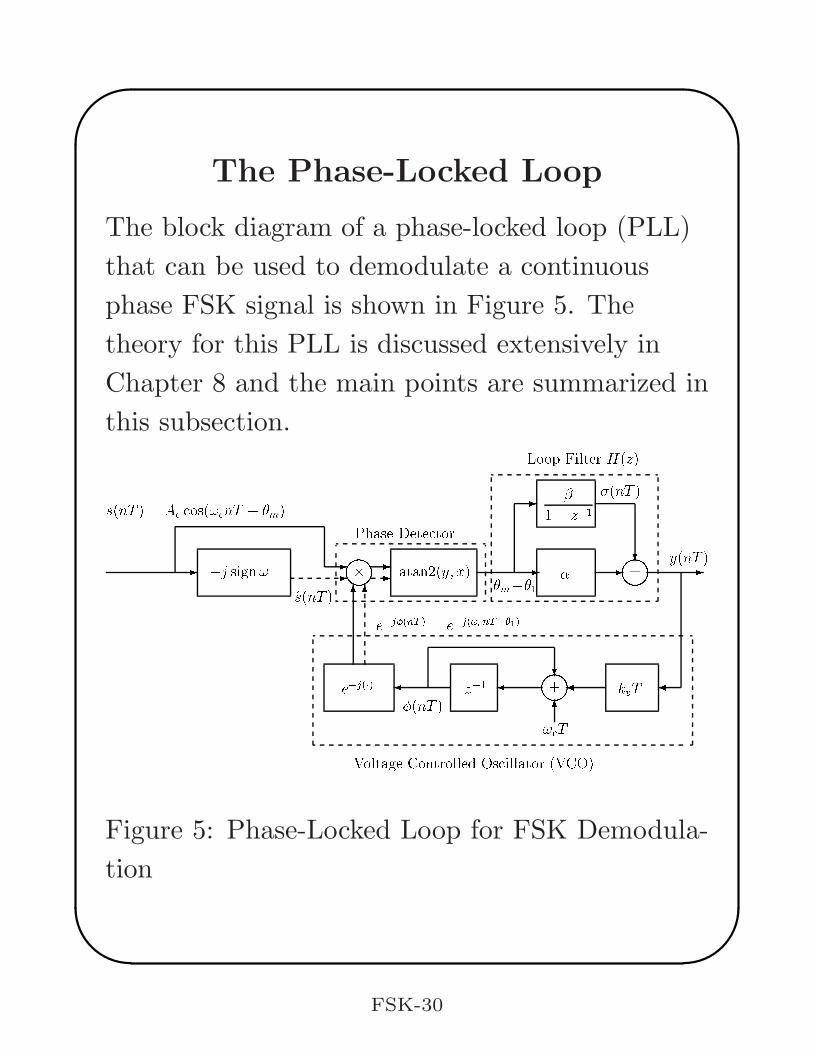
The Phase-Locked Loop
The block diagram of a phase-locked loop (PLL)
that can be used to demodulate a continuous
phase FSK signal is shown in Figure 5. The
theory for this PLL is discussed extensively in
Chapter 8 and the main points are summarized in
this subsection.
-
-
-
-
-
-
?
-
-
-
?
6
66
j sign!
y(nT )
k
v
T
!
c
T
z
1
e
j()
(nT )
+
+
Phase Detector
Voltage Controlled Oscillator (VCO)
e
j(nT )
= e
j(!
c
nT+
1
)
Loop Filter H(z)
s(nT )
atan2(y; x)
(nT )
1 z
1
s(nT ) = A
c
cos(!
c
nT +
m
)
m
1
Figure 5: Phase-Locked Loop for FSK Demodula-
tion
FSK-30
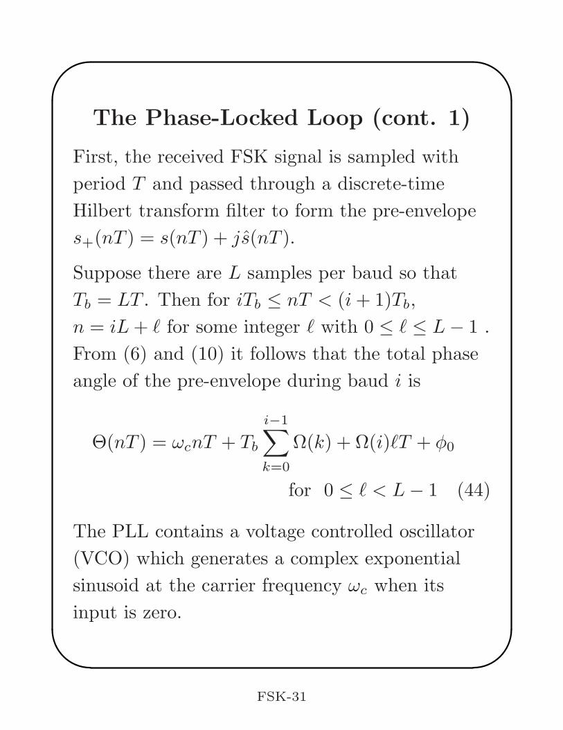
The Phase-Locked Loop (cont. 1)
First, the received FSK signal is sampled with
period T and passed through a discrete-time
Hilbert transform filter to form the pre-envelope
s+(nT ) = s(nT ) + js(nT ).
Suppose there are L samples per baud so that
Tb = LT . Then for iTb ≤ nT < (i+ 1)Tb,
n = iL+ ℓ for some integer ℓ with 0 ≤ ℓ ≤ L− 1 .
From (6) and (10) it follows that the total phase
angle of the pre-envelope during baud i is
Θ(nT ) = ωcnT + Tb
i−1∑
k=0
Ω(k) + Ω(i)ℓT + φ0
for 0 ≤ ℓ < L− 1 (44)
The PLL contains a voltage controlled oscillator
(VCO) which generates a complex exponential
sinusoid at the carrier frequency ωc when its
input is zero.
FSK-31
The Phase-Locked Loop (cont. 2)
The PLL acts to make the VCO total angle
φ(nT ) = ωcnT + θ1(nT ) equal to the angle of the
pre-envelope.
The multiplier in the Phase Detector box
demodulates the pre-envelope using the replica
complex exponential carrier generated by the
VCO.
The phase error between the angles of the
pre-envelope and replica carrier is computed by
the C arctangent function atan2(y, x) where y is
the imaginary part of the multiplier output and x
is its real part.
The parameters α and β in the Loop Filter are
positive constants. Typically, β < α/50 to make
the loop have a tranient response to a phase step
without excessive overshoot.
FSK-32
The Phase-Locked Loop (cont. 3)
The accumulator generating σ(nT ) is included so
that the loop will track a carrier frequency offset.
The parameter kv is also a positive constant. The
product, αkvT , controls the tracking speed of the
loop. It should be large enough so the loop tracks
the input phase changes, but small enough so the
loop is stable and not strongly influenced by
additive input noise.
The VCO generates its phase angle by the
following recursion:
φ(nT + T ) = φ(nT ) + ωcT + kvTy(nT ) (45)
Therefore
kvy(nT ) =φ(nT + T )− φ(nT )
T− ωc (46)
During baud i and assuming the loop is perfectly
in lock so that Θ(nT ) = φ(nT ), substituting
Θ(nT ) given by (44) for φ(nT ) into (46) gives
FSK-33
The Phase-Locked Loop (cont. 4)
kvy(nT ) =Θ(nT + T )−Θ(nT )
T−ωc = Ω(i) (47)
Therefore, the PLL is an FSK demodulator.
When the loop is in lock and the phase error is
small, atan2(x, y) can be closely approximated by
the imaginary part of the complex multiplier
output divided by Ac. The multiplier output is
[s(nT ) + js(nT )]e−jφ(nT ) =
Acej[ωcnT+θm(nT )]e−jφ(nT )
= Acej[φm(nT )−θ1(nT )] (48)
and its imaginary part is
s(nT ) cosφ(nT )− s(nT ) sinφ(nT )
= Ac sin[φm(nT )−θ1(nT )] ≃ Ac[φm(nT )−θ1(nT )]
(49)
where Ac = |s(nT ) + js(nT )|.
FSK-34
The Phase-Locked Loop (cont. 5)
The imaginary part can be divided by the
computed Ac or this scaling can be accomplished
by an automatic gain control (AGC) in the
receiver or by adjusting the loop parameters. The
loop gain in the PLL and, hence, its transient
response depend on Ac if the approximation (49)
is used, so this normalization by Ac is important.
The atan2(y, x) function automatically does the
normalization.
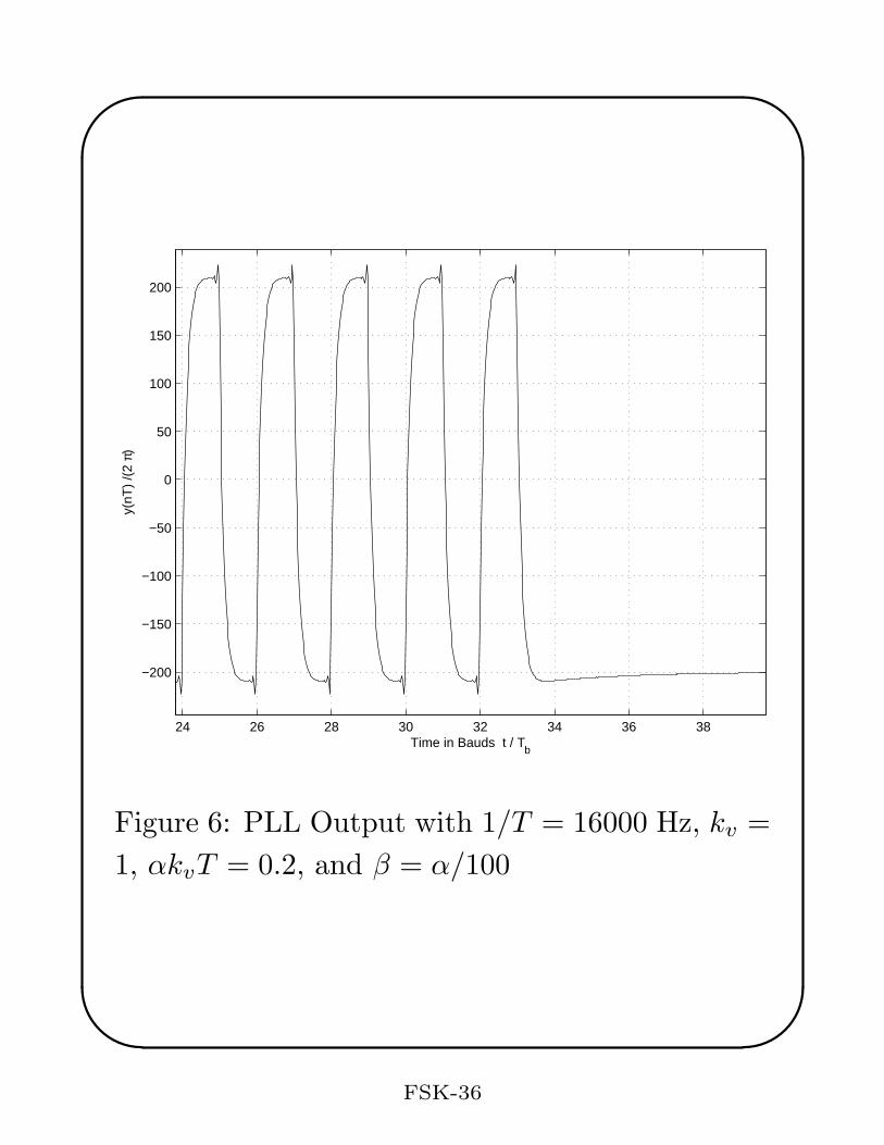
An example of the PLL behavior is shown in
Figure 6 for a binary FSK input signal. The
binary data input to the modulator was a PN
sequence generated by a 23-stage feedback shift
register. The carrier frequency was 4 kHz, the
frequency deviation was 200 Hz, and the baud
rate was 400 Hz. The output shows a segment
where the input alternated between 0 and 1
followed by a string of 1’s.
FSK-35
24 26 28 30 32 34 36 38
−200
−150
−100
−50
0
50
100
150
200
Time in Bauds t / Tb
y(nT
) /(
2 π)
Figure 6: PLL Output with 1/T = 16000 Hz, kv =
1, αkvT = 0.2, and β = α/100
FSK-36
Optimum Noncoherent Detection by
Tone Filters
• The FM discriminator performs very poorly
when the SNR is low or the FSK signal is
distorted, for example, by a speech compression
codec in a cell phone, because differentiation
emphasizes noise.
• The phase-locked loop demodulator performs
better than the discriminator at low SNR but can
have difficulty locking on to FSK signals that are
present in short bursts.
• A better detector for these cases that uses “tone
filters” will now be described . This approach
does not use knowledge of the carrier phase and is
called noncoherent detection.
• A result in detection theory is that in the
presence of additive white Gaussian noise the
detection strategy that is optimum in the sense of
minimizing the symbol error probability for
FSK-37
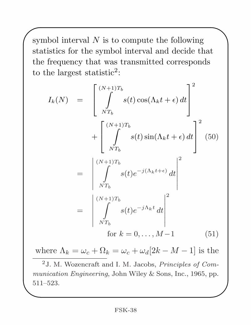
symbol interval N is to compute the following
statistics for the symbol interval and decide that
the frequency that was transmitted corresponds
to the largest statistic2:
Ik(N) =
(N+1)Tb∫
NTb
s(t) cos(Λkt+ ǫ) dt
2
+
(N+1)Tb∫
NTb
s(t) sin(Λkt+ ǫ) dt
2
(50)
=
∣
∣
∣
∣
∣
∣
∣
(N+1)Tb∫
NTb
s(t)e−j(Λkt+ǫ) dt
∣
∣
∣
∣
∣
∣
∣
2
=
∣
∣
∣
∣
∣
∣
∣
(N+1)Tb∫
NTb
s(t)e−jΛkt dt
∣
∣
∣
∣
∣
∣
∣
2
for k = 0, . . . ,M−1 (51)
where Λk = ωc +Ωk = ωc + ωd[2k−M − 1] is the
2J. M. Wozencraft and I. M. Jacobs, Principles of Com-
munication Engineering, John Wiley & Sons, Inc., 1965, pp.
511–523.
FSK-38
total tone frequency, s(t) is the noise corrupted
received signal, and ǫ is a conveniently selected
phase angle. Notice that the statistics have the
same value for every choice of ǫ.
Computing Ik(N) Using Oscillators
and Integrators
The receiver could implement (50) in the obvious
way. It could have a set of M oscillators, each
generating an inphase sine wave cosΛkt and a
quadrature sine wave sinΛkt. Then it would
multiply the input, s(t), by the sine waves,
integrate the products over each baud, and form
the sum of the squares of the inphase and
quadrature integrator outputs for each tone
frequency. The receiver would then decide that
the tone frequency corresponding to the largest
statistic was the one that was transmitted for
that baud.
FSK-39
Computing Ik(N) by a Bank of
Filters
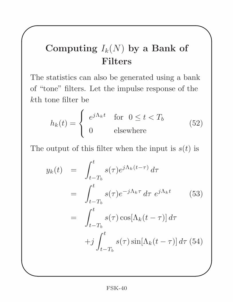
The statistics can also be generated using a bank
of “tone” filters. Let the impulse response of the
kth tone filter be
hk(t) =
ejΛkt for 0 ≤ t < Tb
0 elsewhere(52)
The output of this filter when the input is s(t) is
yk(t) =
∫ t
t−Tb
s(τ)ejΛk(t−τ) dτ
=
∫ t
t−Tb
s(τ)e−jΛkτ dτ ejΛkt (53)
=
∫ t
t−Tb
s(τ) cos[Λk(t− τ)] dτ
+j
∫ t
t−Tb
s(τ) sin[Λk(t− τ)] dτ (54)
FSK-40
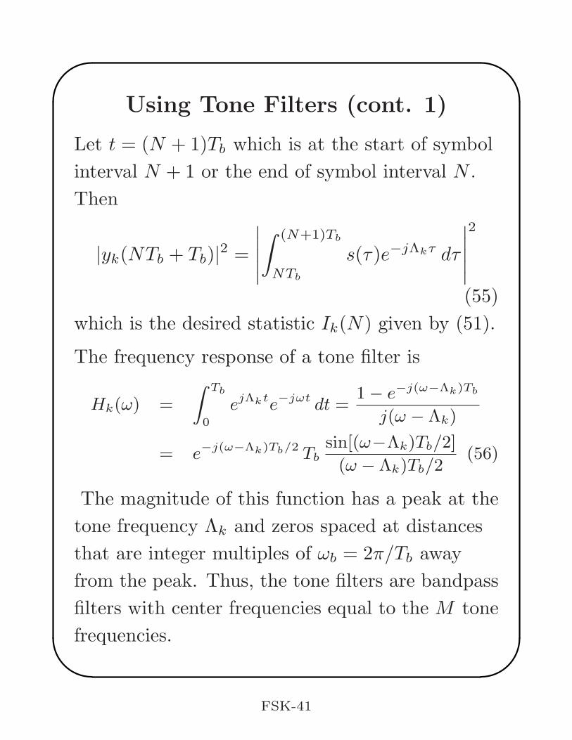
Using Tone Filters (cont. 1)
Let t = (N + 1)Tb which is at the start of symbol
interval N + 1 or the end of symbol interval N .
Then
|yk(NTb + Tb)|2 =
∣
∣
∣
∣
∣
∫ (N+1)Tb
NTb
s(τ)e−jΛkτ dτ
∣
∣
∣
∣
∣
2
(55)
which is the desired statistic Ik(N) given by (51).
The frequency response of a tone filter is
Hk(ω) =
∫ Tb
0
ejΛkte−jωt dt =1− e−j(ω−Λk)Tb
j(ω − Λk)
= e−j(ω−Λk)Tb/2 Tbsin[(ω−Λk)Tb/2]
(ω − Λk)Tb/2(56)
The magnitude of this function has a peak at the
tone frequency Λk and zeros spaced at distances
that are integer multiples of ωb = 2π/Tb away
from the peak. Thus, the tone filters are bandpass
filters with center frequencies equal to the M tone
frequencies.
FSK-41
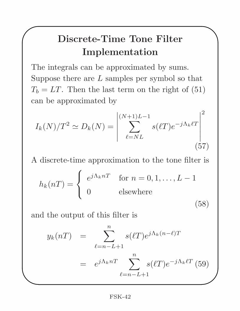
Discrete-Time Tone Filter
Implementation
The integrals can be approximated by sums.
Suppose there are L samples per symbol so that
Tb = LT . Then the last term on the right of (51)
can be approximated by
Ik(N)/T 2 ≃ Dk(N) =
∣
∣
∣
∣
∣
∣
(N+1)L−1∑
ℓ=NL
s(ℓT )e−jΛkℓT
∣
∣
∣
∣
∣
∣
2
(57)
A discrete-time approximation to the tone filter is
hk(nT ) =
ejΛknT for n = 0, 1, . . . , L− 1
0 elsewhere
(58)
and the output of this filter is
yk(nT ) =
n∑
ℓ=n−L+1
s(ℓT )ejΛk(n−ℓ)T
= ejΛknTn∑
ℓ=n−L+1
s(ℓT )e−jΛkℓT (59)
FSK-42
Discrete-Time Tone Filter
Implementation (cont. 1)
Notice that each of the M tone filter impulse
responses is convolved with the same set of L
samples s(ℓT )nℓ=n−L+1. Therefore, an efficient
implementation in terms of minimum memory
usage should have only one delay line containing
these L samples.
The decision statistics for symbol interval N are
obtained at the end of this interval by letting
n = (N + 1)L− 1 in (59) to get
Dk(N) = |yk[(N + 1)LT − T ]|2
=
∣
∣
∣
∣
∣
∣
(N+1)L−1∑
ℓ=NL
s(ℓT )e−jΛkℓT
∣
∣
∣
∣
∣
∣
2
(60)
FSK-43
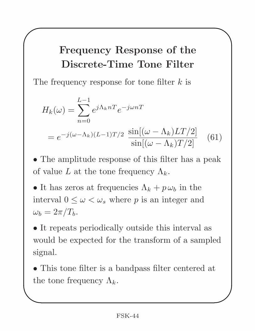
Frequency Response of the
Discrete-Time Tone Filter
The frequency response for tone filter k is
Hk(ω) =
L−1∑
n=0
ejΛknT e−jωnT
= e−j(ω−Λk)(L−1)T/2 sin[(ω − Λk)LT/2]
sin[(ω − Λk)T/2](61)
• The amplitude response of this filter has a peak
of value L at the tone frequency Λk.
• It has zeros at frequencies Λk + pωb in the
interval 0 ≤ ω < ωs where p is an integer and
ωb = 2π/Tb.
• It repeats periodically outside this interval as
would be expected for the transform of a sampled
signal.
• This tone filter is a bandpass filter centered at
the tone frequency Λk.
FSK-44
Block Diagram of Receiver Using
Tone Filters
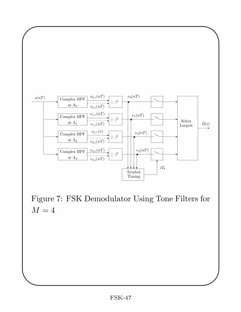
The block diagram of a receiver using tone filters
is shown in Figure 7 for M = 4.
• The boxes labelled “Complex BPF” are the
tone filters.
• The solid line at the output of a box is the real
part of the output and the dotted line is the
imaginary part.
• The boxes labelled | · | form the squared
complex magnitudes of their inputs. These
squared magnitudes are the squared envelopes of
the tone filter outputs.
• The squared envelopes are sampled at the end
of each symbol period, the largest is found, and
the corresponding frequency deviation is assumed
to be the one that was actually transmitted. This
decision is then mapped back to the
corresponding bit pattern.
FSK-45
Efficient Computation with FIR
Tone Filters
If the receiver has locked its local symbol clock
frequency to that of the received signal and the
phase for sampling at the end of a symbol has
been determined, then
• the convolution sum in (59) only has to be
computed at the sampling times.
• In between sampling times, new samples must
be shifted into the filter delay line but the output
does not have to be computed.
• In practice the clocks will continually drift and
must be tracked. The block diagram indicates
that the tone filter outputs are computed for each
new input sample. It will be shown below how a
signal for clock tracking can be derived from these
signals.
FSK-46
e2(nT )
Ω(i)Largest
Select
s(nT )
at Λ2
at Λ3
Complex BPF
Complex BPF
Complex BPF
v0,i(nT )
v0,r(nT )
v1,r(nT )
v2,r(n)
v3,r(nT )
v1,i(nT )
v2,i(nT )
v4,i(nT )
e0(nT )
at Λ1
Complex BPF
at Λ0| · |2
| · |2
| · |2
| · |2
SymbolTiming
•
•
•
•
iTb
e3(nT )
e1(nT )
Figure 7: FSK Demodulator Using Tone Filters for
M = 4
FSK-47
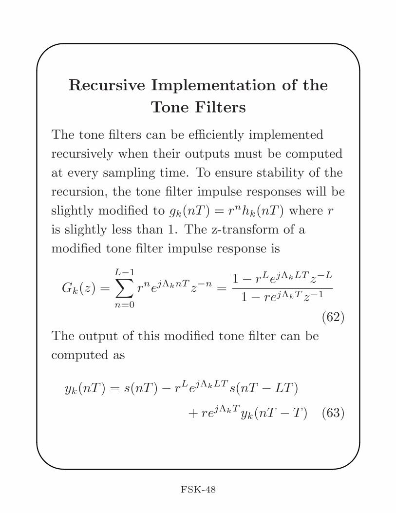
Recursive Implementation of the
Tone Filters
The tone filters can be efficiently implemented
recursively when their outputs must be computed
at every sampling time. To ensure stability of the
recursion, the tone filter impulse responses will be
slightly modified to gk(nT ) = rnhk(nT ) where r
is slightly less than 1. The z-transform of a
modified tone filter impulse response is
Gk(z) =
L−1∑
n=0
rnejΛknT z−n =1− rLejΛkLT z−L
1− rejΛkT z−1
(62)
The output of this modified tone filter can be
computed as
yk(nT ) = s(nT )− rLejΛkLT s(nT − LT )
+ rejΛkT yk(nT − T ) (63)
FSK-48
Recursive Implementation of the
Tone Filters (cont. 1)
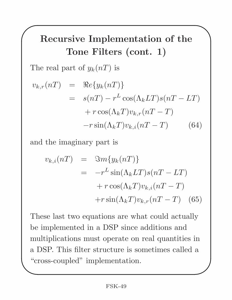
The real part of yk(nT ) is
vk,r(nT ) = ℜeyk(nT )
= s(nT )− rL cos(ΛkLT )s(nT − LT )
+ r cos(ΛkT )vk,r(nT − T )
−r sin(ΛkT )vk,i(nT − T ) (64)
and the imaginary part is
vk,i(nT ) = ℑmyk(nT )
= −rL sin(ΛkLT )s(nT − LT )
+ r cos(ΛkT )vk,i(nT − T )
+r sin(ΛkT )vk,r(nT − T ) (65)
These last two equations are what could actually
be implemented in a DSP since additions and
multiplications must operate on real quantities in
a DSP. This filter structure is sometimes called a
“cross-coupled” implementation.
FSK-49
Computation for the Recursive
Implementation
The quantities rL cos(ΛkLT ), rL sin(ΛkLT ),
r cos(ΛkT ), and r sin(ΛkT ) can be precomputed.
• Then, computation of the real and imaginary
outputs for the cross-coupled form requires six
real multiplications and five real additions for
each n.
• Computation by direct convolution requires
2(L− 1) real multiplications and 2(L− 1) real
additions for each n since hk(0) = gk(0) = 1 and
this is usually much larger than the computation
required for the cross-coupled form.
• The signal memory required for the
cross-coupled form is an L+ 1 word buffer to
store the real values s(ℓT )nℓ=n−L plus two
locations to store vk,r(nT − T ) and vk,i(nT − T ).
This is just slightly more than required by the
direct convolution method.
FSK-50
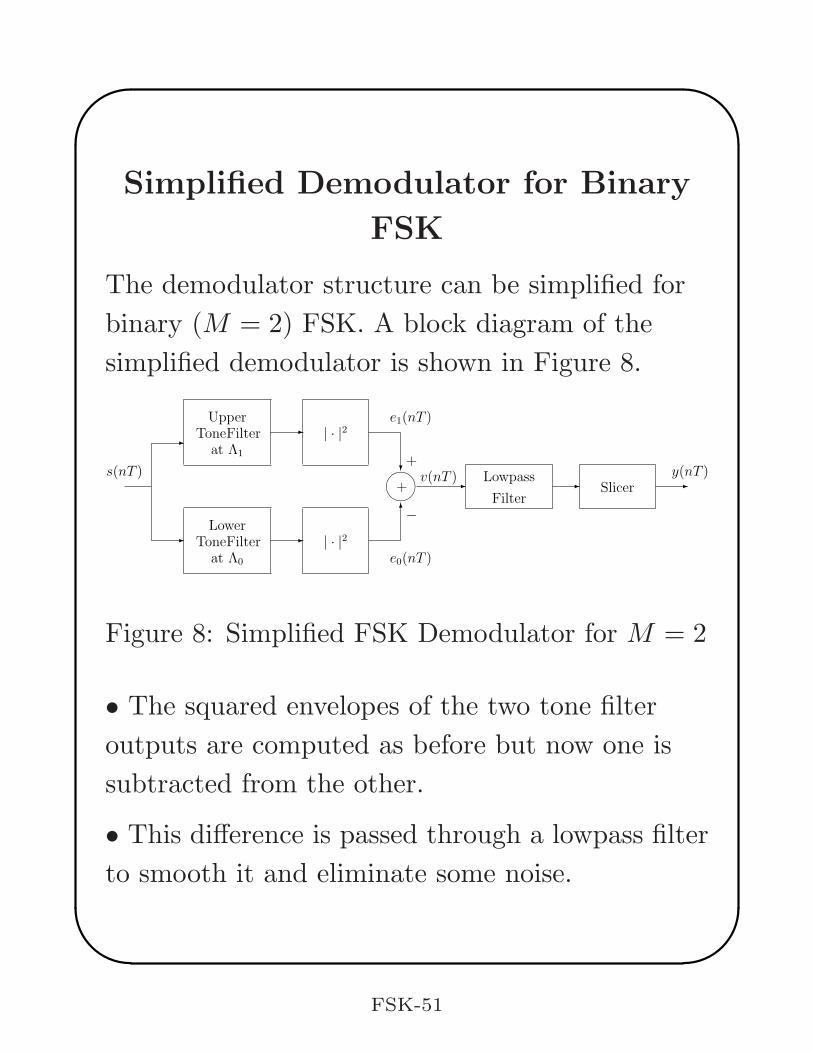
Simplified Demodulator for Binary
FSK
The demodulator structure can be simplified for
binary (M = 2) FSK. A block diagram of the
simplified demodulator is shown in Figure 8.
y(nT )
at Λ1
at Λ0
e1(nT )
e0(nT )
v(nT )Slicer
Upper
Lower
| · |2
| · |2
+
−
+s(nT )
Filter
Filter
Tone
Tone
Lowpass
Filter
Figure 8: Simplified FSK Demodulator for M = 2
• The squared envelopes of the two tone filter
outputs are computed as before but now one is
subtracted from the other.
• This difference is passed through a lowpass filter
to smooth it and eliminate some noise.
FSK-51
Simplified Demodulator for Binary
FSK (cont.)
• The slicer hard limits its input to a positive
voltage A if its input is positive and to a negative
voltage −A if its input is negative.
• When no noise is present on the transmission
channel, a slicer output of A indicates that the
frequency deviation Ω1 was transmitted and an
output of −A indicates that Ω0 was transmitted
during the symbol interval.
Generating a Symbol Clock Timing
Signal
In a low noise environment and when the system
filters are wideband, the symbol clock can be
tracked by locking to the sharp transitions in the
demodulator output.
This will not work in a high noise environment
and when the system filters cause gradual
transitions.
FSK-52
Generating a Symbol Clock Timing
Signal (cont. 1)
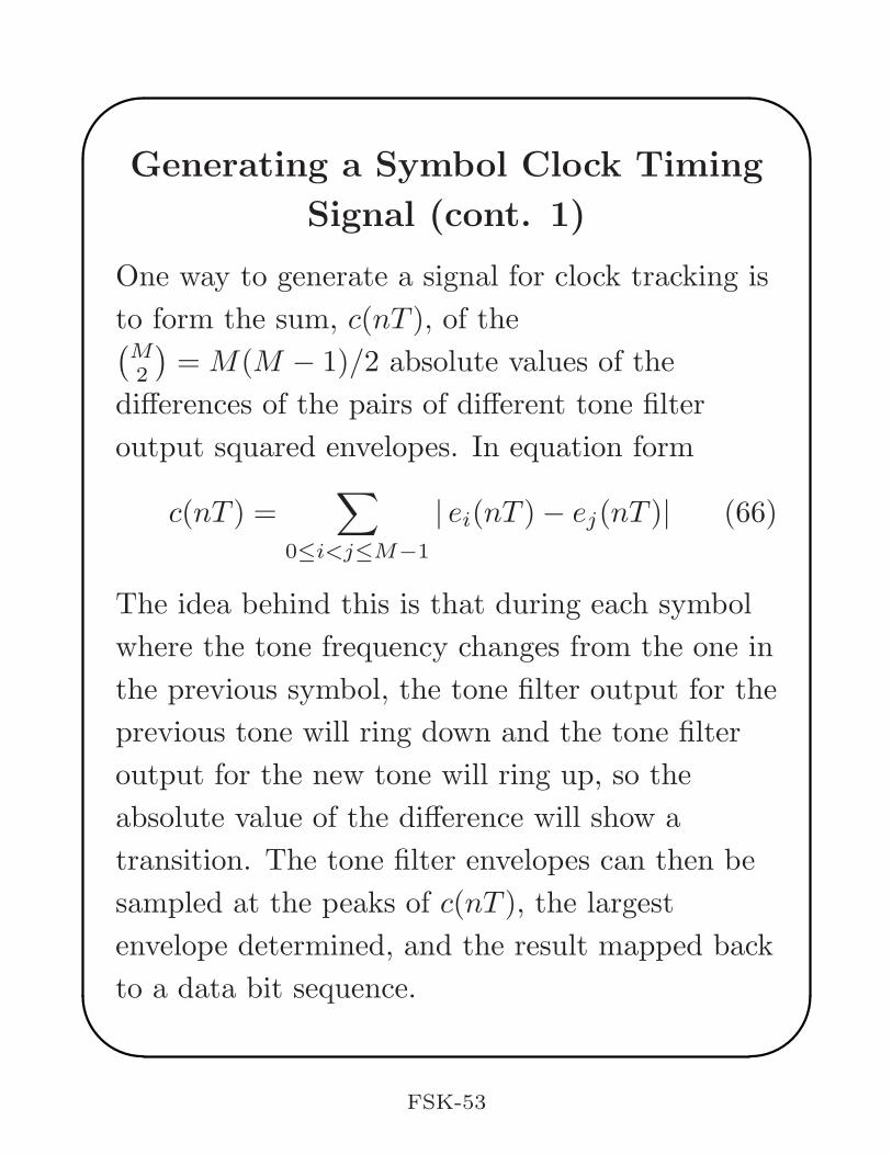
One way to generate a signal for clock tracking is
to form the sum, c(nT ), of the(
M2
)
= M(M − 1)/2 absolute values of the
differences of the pairs of different tone filter
output squared envelopes. In equation form
c(nT ) =∑
0≤i<j≤M−1
| ei(nT )− ej(nT )| (66)
The idea behind this is that during each symbol
where the tone frequency changes from the one in
the previous symbol, the tone filter output for the
previous tone will ring down and the tone filter
output for the new tone will ring up, so the
absolute value of the difference will show a
transition. The tone filter envelopes can then be
sampled at the peaks of c(nT ), the largest
envelope determined, and the result mapped back
to a data bit sequence.
FSK-53
Adding a Bandpass Filter to the
Clock Tracker
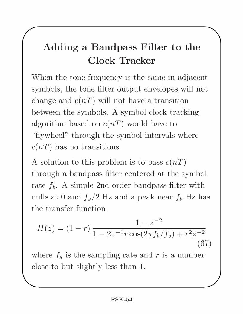
When the tone frequency is the same in adjacent
symbols, the tone filter output envelopes will not
change and c(nT ) will not have a transition
between the symbols. A symbol clock tracking
algorithm based on c(nT ) would have to
“flywheel” through the symbol intervals where
c(nT ) has no transitions.
A solution to this problem is to pass c(nT )
through a bandpass filter centered at the symbol
rate fb. A simple 2nd order bandpass filter with
nulls at 0 and fs/2 Hz and a peak near fb Hz has
the transfer function
H(z) = (1− r)1− z−2
1− 2z−1r cos(2πfb/fs) + r2z−2
(67)
where fs is the sampling rate and r is a number
close to but slightly less than 1.
FSK-54
Adding a Bandpass Filter to the
Clock Tracker (cont. 1)
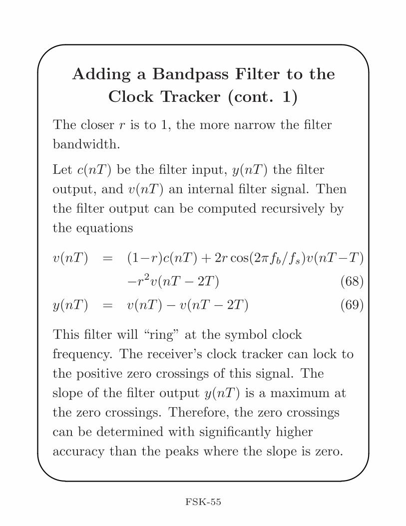
The closer r is to 1, the more narrow the filter
bandwidth.
Let c(nT ) be the filter input, y(nT ) the filter
output, and v(nT ) an internal filter signal. Then
the filter output can be computed recursively by
the equations
v(nT ) = (1−r)c(nT ) + 2r cos(2πfb/fs)v(nT−T )
−r2v(nT − 2T ) (68)
y(nT ) = v(nT )− v(nT − 2T ) (69)
This filter will “ring” at the symbol clock
frequency. The receiver’s clock tracker can lock to
the positive zero crossings of this signal. The
slope of the filter output y(nT ) is a maximum at
the zero crossings. Therefore, the zero crossings
can be determined with significantly higher
accuracy than the peaks where the slope is zero.
FSK-55
Adding a Bandpass Filter to the
Clock Tracker (cont. 2)
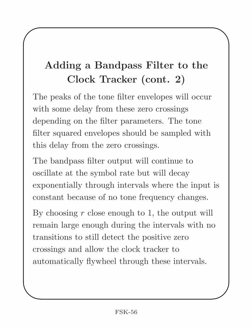
The peaks of the tone filter envelopes will occur
with some delay from these zero crossings
depending on the filter parameters. The tone
filter squared envelopes should be sampled with
this delay from the zero crossings.
The bandpass filter output will continue to
oscillate at the symbol rate but will decay
exponentially through intervals where the input is
constant because of no tone frequency changes.
By choosing r close enough to 1, the output will
remain large enough during the intervals with no
transitions to still detect the positive zero
crossings and allow the clock tracker to
automatically flywheel through these intervals.
FSK-56
Detecting the Presence of an FSK
Signal
The presence of an FSK signal can be detected by
monitoring the sum of the M squared envelopes
ρ(nT ) =
M−1∑
k=0
ek(nT ) (70)
This sum indicates the power received in the tone
filter pass bands. Detection of an FSK signal can
be declared when ρ(nT ) exceeds a threshold for
one or more samples.
The termination of an FSK signal can be declared
when the sum falls below a threshold. The
termination threshold can be set below the
detection threshold to allow hysteresis and reduce
false loss of signal detection.
FSK-57
An M = 4 FSK Example Using Tone
Filters
Typical signals for an M = 4 FSK signal with
fd = 200 Hz, fc = 4000 Hz, fb = 400 Hz,
fs = 16000 Hz, and tone filter detection are
shown in Figures 9, 10, 11, 12, and 13. The tone
frequencies are 3400, 3800, 4200, and 4600 Hz.
For the tone filters r = 0.999 and for the clock
bandpass filter r = 0.998.
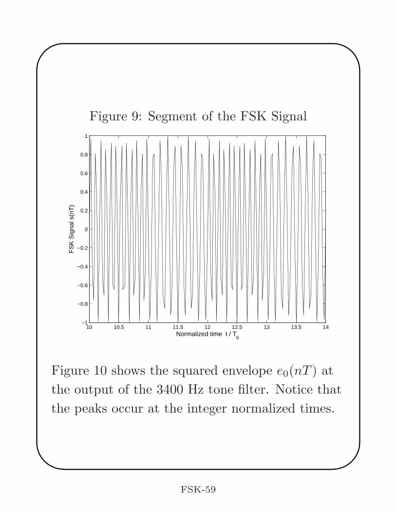
Figure 9 shows a small segment of the FSK signal.
The tone frequency for symbols during normalized
times 10 to 11 and 12 to 13 is 4600 Hz. The tone
frequency during times 11 to 12 and 13 to 14 is
3400 Hz. The varying amplitudes is an optical
illusion created by connecting samples of the
signal taken at a 16000 Hz rate with straight lines.
FSK-58
Figure 9: Segment of the FSK Signal
10 10.5 11 11.5 12 12.5 13 13.5 14−1
−0.8
−0.6
−0.4
−0.2
0
0.2
0.4
0.6
0.8
1
Normalized time t / Tb
FS
K S
igna
l s(n
T)
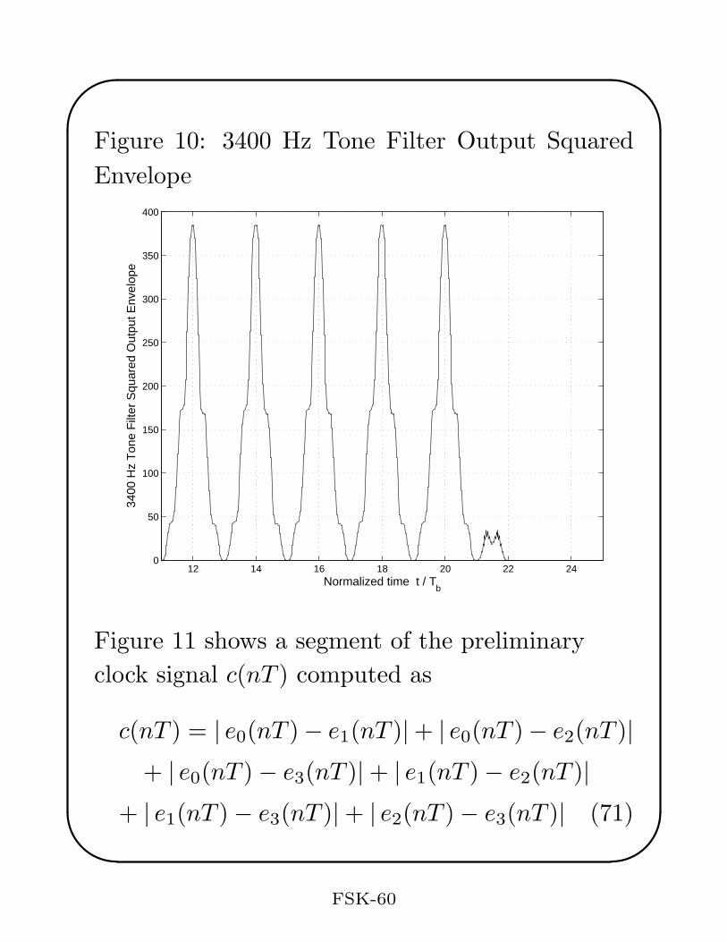
Figure 10 shows the squared envelope e0(nT ) at
the output of the 3400 Hz tone filter. Notice that
the peaks occur at the integer normalized times.
FSK-59
Figure 10: 3400 Hz Tone Filter Output Squared
Envelope
12 14 16 18 20 22 240
50
100
150
200
250
300
350
400
Normalized time t / Tb
3400
Hz
Ton
e F
ilter
Squ
ared
Out
put E
nvel
ope
Figure 11 shows a segment of the preliminary
clock signal c(nT ) computed as
c(nT ) = | e0(nT )− e1(nT )|+ | e0(nT )− e2(nT )|
+ | e0(nT )− e3(nT )|+ | e1(nT )− e2(nT )|
+ | e1(nT )− e3(nT )|+ | e2(nT )− e3(nT )| (71)
FSK-60
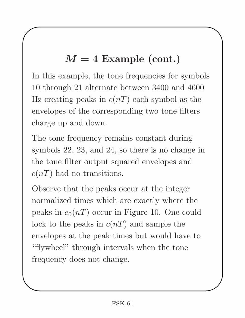
M = 4 Example (cont.)
In this example, the tone frequencies for symbols
10 through 21 alternate between 3400 and 4600
Hz creating peaks in c(nT ) each symbol as the
envelopes of the corresponding two tone filters
charge up and down.
The tone frequency remains constant during
symbols 22, 23, and 24, so there is no change in
the tone filter output squared envelopes and
c(nT ) had no transitions.
Observe that the peaks occur at the integer
normalized times which are exactly where the
peaks in e0(nT ) occur in Figure 10. One could
lock to the peaks in c(nT ) and sample the
envelopes at the peak times but would have to
“flywheel” through intervals when the tone
frequency does not change.
FSK-61
Figure 11: The Preliminary Symbol Clock Track-
ing Signal c(nT )
10 12 14 16 18 20 22 240
200
400
600
800
1000
1200
Normalized time t / Tb
Pre
limin
ary
Clo
ck S
igna
l c(n
T)
FSK-62
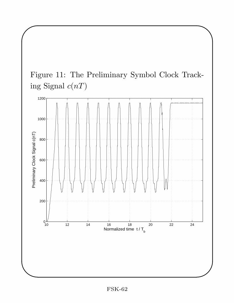
Figure 12: The Signal c(nT ) Passed through a 2nd
Order Bandpass Filter
16 18 20 22 24 26 28 30 32 34 36 38−300
−200
−100
0
100
200
300
Normalized time t / Tb
Ban
dpas
s F
ilter
ed P
relim
inar
y C
lock
Sig
nal y
(nT
)
Figure 12 shows the result when c(nT ) is passed
through the bandpass filter centered at the
symbol clock frequency. Notice that the signal is
exponentially damped between normalized times
22 and 30 when c(nT ) has no transitions.
FSK-63
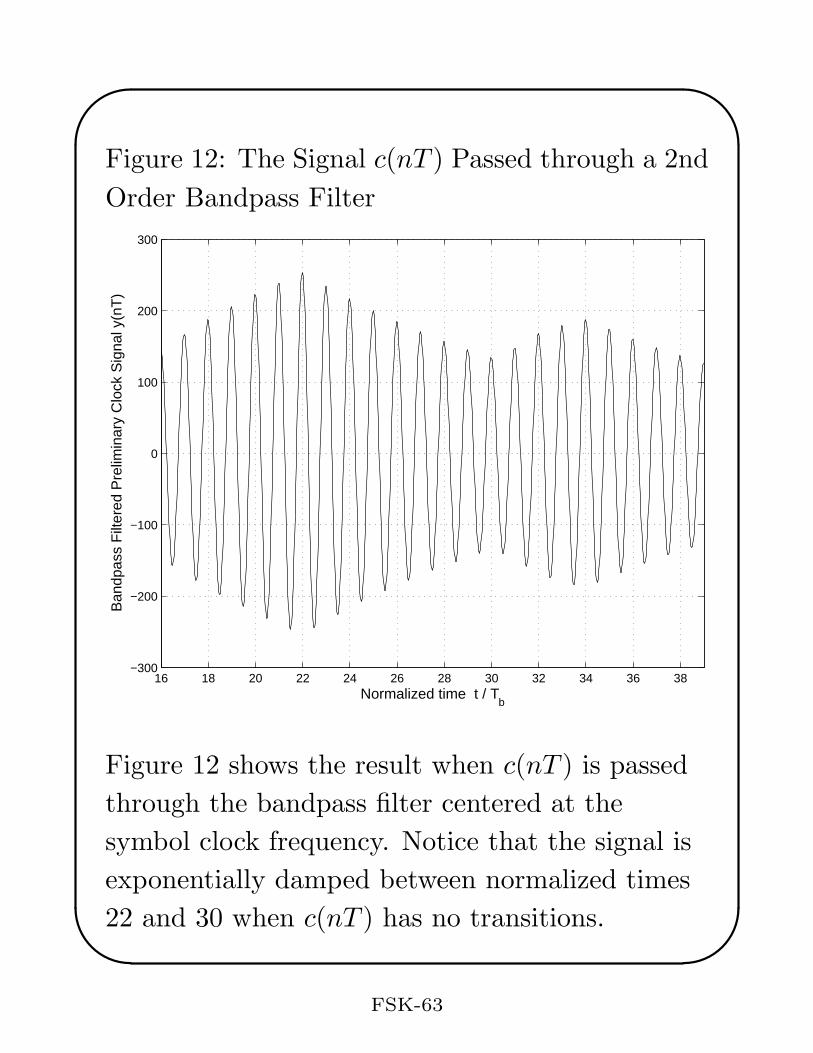
Figure 13: Superimposed Preliminary and Band-
pass Filtered Clock Signals
19 19.5 20 20.5 21 21.5 22 22.5 23−300
−200
−100
0
100
200
300
Normalized time t / Tb
c(nT)/4y(nT)
Figure 13 shows a segment of the preliminary
clock signal, c(nT ), and the bandpass filtered
clock signal, y(nT ), superimposed on the same
graph. The peaks of y(nT ) occur at almost the
same times as the peaks in c(nT ).
FSK-64
The positive zero crossings of y(nT ) occur 1/4 of
a symbol before the peaks of c(nT ). A good clock
tracker would lock to these zero crossing and the
receiver would then sample the tone filter squared
envelopes with a delay of 1/4 of a symbol which
corresponds to the peaks of c(nT ). The exact
delay necessary depends on the filter parameters.
Symbol Error Probabilities for FSK
Systems
The problem of computing the symbol error
probability for different types of FSK receivers is
discussed extensively in Chapter 8 of Lucky, Salz,
and Weldon3. The problem is very difficult
because of the nonlinear natures of the modulator
and various receivers. Many of the results are
approximations or require evaluation of
complicated integrals by numerical integration.
3R.W. Lucky, J. Salz, and E.J. Weldon, Principles of
Data Communication, McGraw-Hill Book Company, 1968
FSK-65
Orthogonal Signal Sets
One case where exact closed form results are
know is when the transmitted symbols are
orthogonal, they are corrupted by additive white
Gaussian noise, and optimum noncoherent
detection by tone filters is used.
Two continuous-time signals over the interval
[t1, t2) with complex envelopes x1(t) and x2(t) are
said to be orthogonal if
ρ =
∫ t2
t1
x1(t)x2(t) dt = 0 (72)
From (13) it follows that the complex envelopes of
the FSK signal set during symbol period i where
iTb ≤ t < (i+ 1)Tb are
xk(t) = Acejθm(iTb)ejωd[2k−(M−1)](t−iTb)
for k = 0, . . . ,M − 1 (73)
FSK-66
Orthogonal Signal Sets (cont. 1)
For two distinct integers k1 and k2 in this set
ρ =
∫ (i+1)Tb
iTb
xk1(t)xk2
(t) dt
= A2c
∫ (i+1)Tb
iTb
ej2ωd(k1−k2)(t−iTb) dt]
= A2c
∫ Tb
0
ej2ωd(k1−k2)t dt
= A2c
ej2ωd(k1−k2)Tb − 1
j2ωd(k1 − k2)(74)
This integral will be zero if
2ωd(k1 − k2)Tb = 2πℓ (75)
or
h(k1 − k2) = ℓ (76)
where ℓ is an integer. This will be satisfied for all
pairs of signals in the FSK signal set when the
modulation index, h, is an integer.
FSK-67
Orthogonal Signal Sets (cont. 2)
An analogous property holds for the discrete-time
FSK approximation. Assume there are L samples
per symbol so that Tb = LT . The complex
discrete-time envelopes during symbol interval i
where iTb ≤ nT < (i+ 1)Tb are
xk(nT ) = Acejθm(iTb)ejωd[2k−(M−1)](nT−iLT )
for k = 0, . . . ,M − 1 (77)
Then for two distinct integers k1 and k2 the
correlation is
ρ =
(i+1)L−1∑
n=iL
xk1(nT )xk2
(nT )
= A2c
L−1∑
n=0
ej2ωd(k1−k2)nT
= A2c
1− ej2ωd(k1−k2)LT
1− ej2ωd(k1−k2)T(78)
The correlation ρ will be zero if
2ωd(k1 − k2)LT = 2ωd(k1 − k2)Tb = 2πℓ where ℓ
is an integer just as in the continuous-time case.
FSK-68
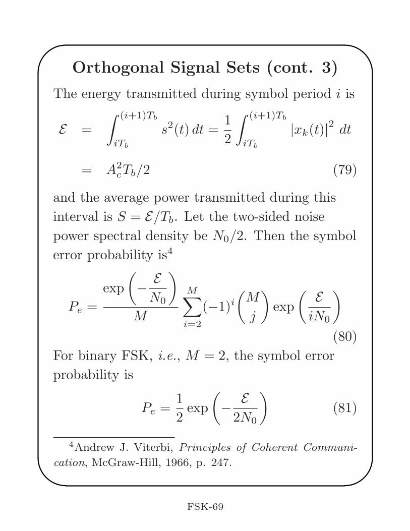
Orthogonal Signal Sets (cont. 3)
The energy transmitted during symbol period i is
E =
∫ (i+1)Tb
iTb
s2(t) dt =1
2
∫ (i+1)Tb
iTb
|xk(t)|2dt
= A2cTb/2 (79)
and the average power transmitted during this
interval is S = E/Tb. Let the two-sided noise
power spectral density be N0/2. Then the symbol
error probability is4
Pe =
exp
(
−E
N0
)
M
M∑
i=2
(−1)i(
M
j
)
exp
(
E
iN0
)
(80)
For binary FSK, i.e., M = 2, the symbol error
probability is
Pe =1
2exp
(
−E
2N0
)
(81)
4Andrew J. Viterbi, Principles of Coherent Communi-
cation, McGraw-Hill, 1966, p. 247.
FSK-69
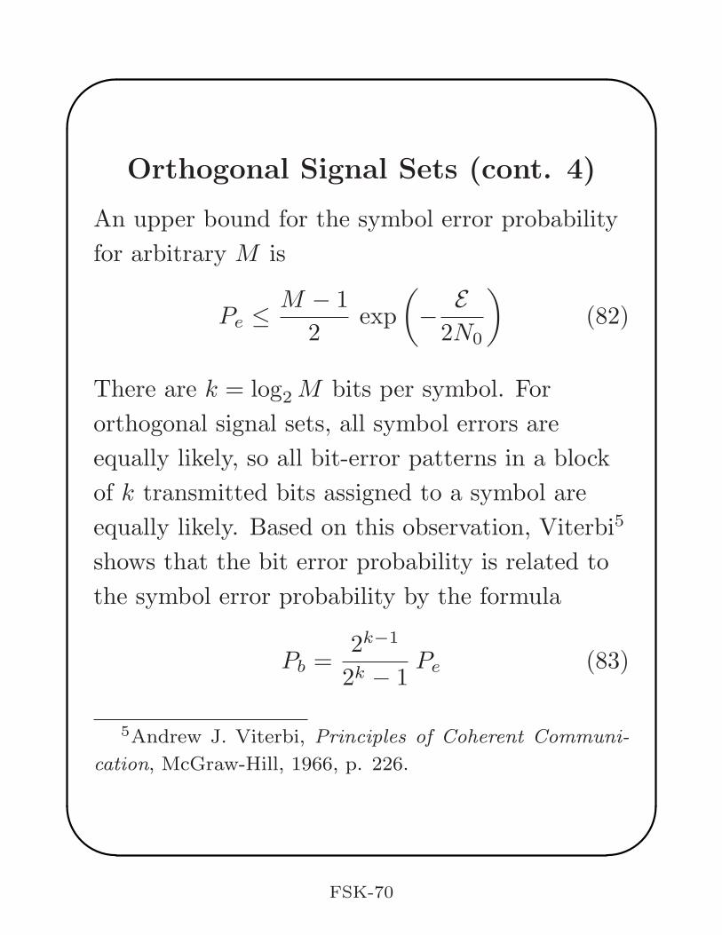
Orthogonal Signal Sets (cont. 4)
An upper bound for the symbol error probability
for arbitrary M is
Pe ≤M − 1
2exp
(
−E
2N0
)
(82)
There are k = log2 M bits per symbol. For
orthogonal signal sets, all symbol errors are
equally likely, so all bit-error patterns in a block
of k transmitted bits assigned to a symbol are
equally likely. Based on this observation, Viterbi5
shows that the bit error probability is related to
the symbol error probability by the formula
Pb =2k−1
2k − 1Pe (83)
5Andrew J. Viterbi, Principles of Coherent Communi-
cation, McGraw-Hill, 1966, p. 226.
FSK-70
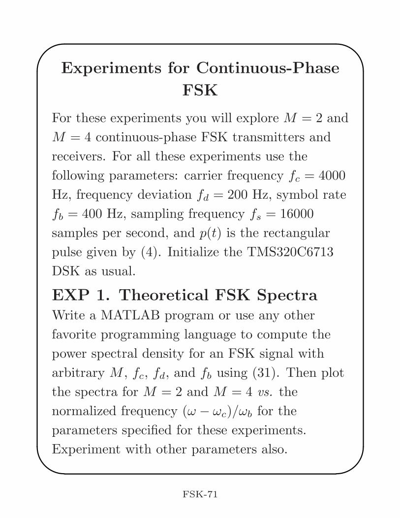
Experiments for Continuous-Phase
FSK
For these experiments you will explore M = 2 and
M = 4 continuous-phase FSK transmitters and
receivers. For all these experiments use the
following parameters: carrier frequency fc = 4000
Hz, frequency deviation fd = 200 Hz, symbol rate
fb = 400 Hz, sampling frequency fs = 16000
samples per second, and p(t) is the rectangular
pulse given by (4). Initialize the TMS320C6713
DSK as usual.
EXP 1. Theoretical FSK SpectraWrite a MATLAB program or use any other
favorite programming language to compute the
power spectral density for an FSK signal with
arbitrary M , fc, fd, and fb using (31). Then plot
the spectra for M = 2 and M = 4 vs. the
normalized frequency (ω − ωc)/ωb for the
parameters specified for these experiments.
Experiment with other parameters also.
FSK-71
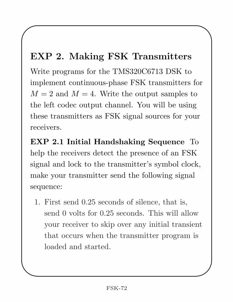
EXP 2. Making FSK Transmitters
Write programs for the TMS320C6713 DSK to
implement continuous-phase FSK transmitters for
M = 2 and M = 4. Write the output samples to
the left codec output channel. You will be using
these transmitters as FSK signal sources for your
receivers.
EXP 2.1 Initial Handshaking Sequence To
help the receivers detect the presence of an FSK
signal and lock to the transmitter’s symbol clock,
make your transmitter send the following signal
sequence:
1. First send 0.25 seconds of silence, that is,
send 0 volts for 0.25 seconds. This will allow
your receiver to skip over any initial transient
that occurs when the transmitter program is
loaded and started.
FSK-72
2. Then for M = 2 send 25 symbols alternating
each symbol between f0 = 3800 and
f1 = 4200 Hz tones. This will allow the
receivers to detect the FSK signal and lock on
to the symbol clock. For M = 4 send 25
symbols alternating each symbol between
f0 = 3400 and f3 = 4600 Hz.
3. Suppose the frequencies of the last few
symbols of the alternating sequence for
M = 2 were · · · , f0, f1, f0. Next send an
alternating frequency sequence for 10 symbols
but with the alternation reversed. That is
send f0, f1, f0, f1, f0, f1, f0, f1, f0, f1. Your
receiver can detect this change in the
alternations and use it as a timing mark to
determine when actual data will start.
For the M = 4 transmitter change to
alternating between f1 = 3800 and f2 = 4200
Hz for 10 symbols. Again, this change can be
used as a timing mark.
FSK-73
EXP 2.2 Simulating Random Customer
Data
After the alternations, begin transmitting
“customer” data continuously.
Simulate this data by using a 23 stage PN
sequence generator as discussed in Chapter 9.
Use the connection polynomial
h(D) = 1 +D18 +D23
so the data bit sequence, d(n), is generated by the
recursion
d(n) = d(n− 18)⊕ d(n− 23) (84)
where “⊕” in the recursion is modulo 2 addition,
that is, the exclusive-or operation. Initialize the
PN sequence generator shift register to some
non-zero state.
For M = 2, shift the PN generator once to get a
new data bit d(n) which will be a 0 or 1. Map
this bit to the tone frequency
Λ(n) = ωc + ωd[2d(n)− 1].
FSK-74
For M = 4, shift the register twice to get a pair of
bits [d1(n), d0(n)]. Consider this bit pair to be the
integer k(n) = 2d1(n) + d0(n) which can be 0, 1,
2, or 3. Map this bit pair to the tone frequency
Λ(n) = ωc + ωd[2k(n)− 3].
EXP 2.3 Experimentally Measure the FSK
Power Spectral Density
Measure the power spectral density of the
transmitted FSK signals for M = 2 and 4 after
the initial handshaking sequence when random
customer data is being transmitted.
• If you made the spectrum analyzer for Chapter
4, run it on one station and connect your
transmitter to it.
• You can use a commercial spectrum analyzer if
it is available.
• Otherwise collect an array of transmitted
samples, write them to a file on the PC, and use
MATLAB’s Signal Processing Toolbox function
pwelch( ). Compare your measured spectra with
the theoretical ones you computed.
FSK-75
EXP 3. Making a Receiver Using an
Exact Frequency Discriminator
Make a receiver using the exact frequency
discriminator shown in Figure 3 for M = 2.
Connect the transmitter from another station to
your receiver. There are RCA-to-RCA barrel
connectors in the cabinet to connect RCA to
mini-stereo cables together.
First leave your transmitter off and turn on your
receiver. When the receiver is running, turn on
your transmitter. Your receiver program should
do the following:
1. The receiver should detect the absence or
presence of an input FSK signal by
monitoring the received signal power. The
power can be calculated by doing a running
average of the squared input samples over
several symbols. You can also try a single
pole exponential averager.
FSK-76
EXP 3. Making an Exact Discriminator
(cont. 1)
The receiver should assume that no FSK
input signal is present when this power is
small and sit in a loop checking for the
presence of an input signal. When the
measured power crosses a threshold, the
receiver can start the discriminator and
symbol clock tracking algorithm.
You should predetermine a good threshold
based on your knowledge of the transmitter
amplitude and system gains. You can do this
experimentally by observing the received
power when the transmitter is running.
2. The receiver should continue to monitor the
input signal power and detect when the signal
is gone and then go into a loop looking for
the return of a signal.
FSK-77
EXP 3. Making an Exact Discriminator
(cont. 2)
3. Start your discriminator and symbol clock
tracker once an input signal is detected.
Monitor the tone frequency alternations and
look for the alternation switch. Count for 10
symbols after the switch and begin detecting
the tone frequencies resulting from the input
customer data.
4. Send the output samples of the discriminator
to the left codec channel.
Send a signal to the right codec output
channel that is a square wave at the symbol
clock frequency to use for synching the
oscilloscope. You can do this by sending a
positive value for 20 samples at the start of a
symbol followed by its negative value for the
next 20 samples.
FSK-78
EXP 3. Making an Exact Discriminator
(cont. 3)
Observe the discriminator output on the
oscilloscope and take a picture of a single
trace to show a typical output of the
discriminator.
Alternatively, you can capture an array of
discriminator output samples with Code
Composer or use fprintf(·) to write the array
to a PC file and plot the output file with your
favorite plotting program.
If you allow the oscilloscope to run freely, you
will see multiple traces synchronized with the
symbol clock overlapped on the screen. This
type of display is called an “eye pattern” in
the communications industry. At the end of
each symbol you should see two distinct equal
and opposite levels and the eye is said to be
open. The eye pattern can be used as a
diagnostic tool. Noise and system problems
cause the eye to be less open.
FSK-79
EXP 3. Making an Exact Discriminator
(cont. 4)
5. Map the detected tone frequency sequence
back into a bit sequence d(n).
6. Check that the received bit stream is the
same as the transmitted one. Your receiver
should have a 24-stage shift register that
contains d(n), d(n− 1), . . . , d(n− 23). You
can check for errors by checking that
d(n)⊕ d(n− 18)⊕ d(n− 23) = 0
for all n except for an initial burst of 1’s when
the shift register is filling up. If you initialize
the state of the register to the initial state of
the transmitter register the result should be
all 0’s if you have detected the starting time
of the customer data correctly.
FSK-80
EXP 4. Running a Bit-Error Rate
Test (BERT)
A measure of the quality of a digital transmission
scheme is its bit-error rate performance in the
presence of additive noise. Once your frequency
discriminator receiver is working correctly with
noiseless received FSK signals, perform a bit-error
rate test as follows:
1. Generate zero-mean Gaussian noise samples
in the DSP with some variance σ2 and add
them to the received signal samples.
Implement a power meter in your receiver
program to measure the power of the FSK
input samples, say P . Compute the SNR =
10 log10(P/σ2) dB.
2. Your receiver should have a replica of the PN
sequence generator in the transmitter. You
should synchronize the state of the local PN
generator to that of the transmitter so it’s
output sequence will be in phase with the
received one.
FSK-81
EXP 4. BERT Test (cont. 1)
3. Start your BERT test with a very high SNR
so few errors will occur. Check if each bit
estimated by the receiver is the same as the
transmitted one and count any bit errors for a
number of bits sufficient to give a good
estimate of the bit-error probability.
The estimated bit-error rate is:
BER = (the number of errors in the observed
sequence of detected bits)/(the number of
observed detected bits).
The number of observed bits should be at
least 10 times the bit-error rate to get an
estimate with good accuracy. The variance of
this estimator decreases inversely with the
number of observed bits.
FSK-82
EXP 4. BERT Test (cont. 2)
4. Decrease the SNR in steps of 0.25 dB and
measure the bit-error rate for each SNR.
Continue decreasing the SNR until you can
no longer synchronize the replica PN
generator with the transmitter’s generator.
5. Plot the bit-error rate vs. SNR. The bit-error
rate should be plotted on a logarithmic scale
and SNR in dB on a linear scale. This kind of
plot is known as a “waterfall curve” in the
communications industry.
EXP 5. Making a Receiver Using an
Approximate Frequency
Discriminator
Repeat the tasks for the exact frequency
discriminator in EXP 3 for the approximate
frequency discriminator presented starting on
slide FSK-25.
FSK-83
EXP 6. Making a Receiver Using a
Phase-Locked Loop
Make a receiver using the phase-locked loop
described starting on Slide FSK-30 for M = 2.
Test your receiver by following the steps starting