Continuum approximations of individual-based models …ojensen/OpenArchive/fozardetal.pdf ·...

Mathematical Medicine and BiologyPage 1 of 36doi:10.1093/imammb/dri000

Continuum approximations of individual-based models for epithelialmonolayers

J.A. FOZARD, H.M. BYRNE, O.E. JENSEN, J.R. KING

School of Mathematical Sciences, University of Nottingham,University Park, Nottingham, NG7 2RD, UK.

This work examines a one-dimensional individual-based model (IBM) for a system of tightly adherentcells, such as an epithelial monolayer. Each cell occupies abounded region, defined by the location of itsendpoints, has both elastic and viscous mechanical properties and is subject to drag generated by adhe-sion to the substrate. Differential-algebraic equations governing the evolution of the system are obtainedfrom energy considerations. This IBM is then approximated by continuum models (systems of partialdifferential equations)in the limit of a large number of cells, N, when the cell parameters vary slowlyin space or are spatially periodic (and so may be heterogeneous, with substantial variation between adja-cent cells). For spatially periodic cell properties with significant cell viscosity, the relationship betweenthe mean cell pressure and length for the continuum model is found to be history-dependent.Termsinvolving convective derivatives, not normally included in continuum tissue models, are identified.The specific problem of the expansion of an aggregate of cellsthrough cell growth (but without division)is considered in detail, including the long-time and slow-growth-rate limits. When the parameters ofneighbouring cells vary slowly in space, theO(1/N2) error in the continuum approximation enables thisapproach to be used even for modest values ofN. In the spatially periodic case, the neglected terms arefound to beO(1/N). The model is also used to examine the acceleration of a wound edge observedin wound-healing assays.

Keywords: Multicellular, homogenization, individual-based, continuum, epithelial, monolayer.

1. Introduction

Epithelial tissues consist of sheets of tightly adherent cells with apicobasal polarization. These coverthe internal and external surfaces of the body and one of their functions is to act as a barrier, regulatingthe migration of cells and chemicals across them (Alberts, 2002). The study of such tissues is impor-tant not only because of their roles in wound healing (Martin, 1997) and morphogenesis (Schock andPerrimon, 2002) but also because the majority of tumours in humans are epithelial in origin. Duringcarcinogenesis in the colon, for example, cells mutate, colonize crypts and develop into a tumour in acomplex series of events (Humphries and Wright, 2008); these involve interactions between multiplecells through mechanical forces, cell adhesion and cell signalling. As a consequence of this complexity,mathematical modelling is necessary to understand the entirety of the process (Anderson and Quaranta,2008).

The cell is a natural unit of organisation in a multicellularsystem. Models for such systems canbe loosely divided into two categories: continuum models and individual- (or agent-) based models.Continuum models describe the properties of the cells in terms of locally averaged quantities (e.g. thenumber density of cells) whose evolution is governed by (partial) differential equations. Individual-based models (IBMs) take a contrasting approach, in which each cell is treated as a distinct entity, withassociated position and properties; these evolve according to rules which depend only on the internalstate and local environment of each cell. There is much variation between IBMs, some of which arereviewed by Brodland (2004), and many different discrete models have been used to study epithelial

c© The author 2008. Published by Oxford University Press on behalf of the Institute of Mathematics and its Applications. All rights reserved.

2 of 36 J.A. FOZARD et al.

tissues (e.g. Bindschadler and McGrath, 2007; Chen and Brodland, 2000; Galle et al., 2005; Meinekeet al., 2001; Nagai and Honda, 2001; Odell et al., 1981; van Leeuwen et al., 2009; Walker et al., 2004;Weliky and Oster, 1990).

The two types of models have relative advantages and disadvantages, the importance of which de-pends on the nature of the system and the biological questionunder consideration. Existing continuummodels fail to resolve details on cellular or subcellular scales (Anderson, 2007), whereas it is relativelystraightforward to include subcellular properties in the framework of an IBM (e.g. gene regulatorynetworks (Ramis-Conde et al., 2008; van Leeuwen et al., 2009), cytoskeletal dynamics (Maree et al.,2006), cell-cycle dynamics (Alarcon et al., 2004), natural selection of cellular phenotypes (Anderson,2007; Hogeweg, 2000)) and cellular processes (e.g. juxtacrine signalling (Savill and Sherratt, 2003)).Similarly, it is simpler to include heterogeneous cell populations in IBMs than in continuum models, andIBMs may be used to model small numbers of cells. However, techniques for the mathematical analysisof continuum models are better developed than those for IBMs. The computational expense of numeri-cal simulations of IBMs depends upon the number of cells in the system, whilst for continuum modelsit depends upon the size of the system relative to the scale onwhich variations of interest occur, as thisdictates the number of variables required for the spatial discretization to give a good approximation tothe continuous solution.

Relating continuum models to IBMs in the limit of large numbers of cells is important for severalreasons. As discussed above, continuum models may be substantially more efficient to simulate thanIBMs, provided that the variations of interest occur over scales which are much larger than the size of thecells. Parameter estimation is a significant problem in biological modelling, and relating the two typesof models may allow measurements of cell-scale properties to be used to estimate parameters in con-tinuum models, and vice-versa. The two types of models have largely been developed in isolation, andconnecting them may motivate developments in models of bothkinds; the choices made in developinga continuum model (number of components, constitutive law,etc.) are often difficult to justify, whilstIBMs require many assumptions about the behaviour of individual cells. In particular, the study of IBMswill be useful in rationalising phenomenological interaction terms such as those arising in multiphasemodels of tissue growth (Lemon et al., 2006).

Continuum approximations of spatially discrete models have been of great interest in physical sci-ence, in particular for lattice models such as the Fermi, Pasta and Ulam model (a chain of particlesconnected by nonlinear springs). By expanding differencesin Taylor series, a continuum approxima-tion was obtained (Kruskal and Zabusky, 1964; Zabusky and Kruskal, 1965), exemplifying a procedurethat is applicable in many such contexts(such as the approximation of discrete systems of masterequations (Keck and Carrier, 1965)); we will show how such approaches cen be extended to modelheterogeneous cell populations below. We do so using homogenization methods (Bensoussan et al.,1978; Pavliotis and Stuart, 2008), which have been applied to many physical processes, notably thesolid mechanics of composite materials (Milton, 2002) and porous media (Hornung, 1997) when theproperties of the medium vary on a small length scale. These methods have also been used in biologicalcontexts, e.g. the bistable equation with heterogeneous conductivity as a model for wave propagationin cardiac tissue (Keener, 2000), models for neural networks (Bressloff, 2001), calcium dynamics inthe cell cytoplasm (Goel et al., 2006) and transport of diffusible substances in a line of coupled cells(Othmer, 1983). The aim of this procedure is to derive equations which govern the behaviour of thesystem over spatial scales which are much larger than those on which the material properties vary; theequations describing large-scale behaviour are often the same as those for the small-scale problem, butwith different effective constitutive relations (averaged over the short length scale). While such methodsare more commonly applied to systems which are spatially continuous, we will here consider a system

Continuum approximation of IBMs 3 of 36

which is discrete in space; as noted in Kevrekidis et al. (2002), such discrete problems can typically bewritten as continuum problems with (heterogeneous) coefficients containing spatial delta functions.

Conversely, the approximation of spatially continuous models by discrete ones is fundamental to thenumerical analysis of partial differential equations. Whilst the spatial discretization is usually chosenbecause it gives a good approximation to the continuum problem, with the resulting discrete equationshaving favourable properties, related techniques used canbe instructive in approximating discrete sys-tems by continuous ones.

Continuum approximations of IBMs have been derived by a number of authors, the results obtainedbeing specific to the particular models. In off-lattice centre-based models, each cell is described by theposition of its centre, the cells exert forces on each other and the velocity of a cell centre is proportionalto the applied force. A one-dimensional model of this type, in which the force between cells dependson the distance between them (with optional additive noise)was examined by Bodnar and Velazquez(2005), and an integro-differential equation governing the cell densities was derived. Alt (2002) con-sidered a two-dimensional model in which only neighbouringcells interact (these being determinedby the Voronoi diagram based on the cell centres), the forcesbetween cells depending on the distancebetween them, the relative velocity and the length of the common side in the Voronoi tessellation; acontinuity equation for the cell density and a Navier–Stokes-type force-balance equation with additivenoise for the cell velocities were conjectured. This approximation has been derived rigorously for theone-dimensional version of this model by Albeverio and Alt (2008). Drasdo (2005) derived a continuumapproximation for an off-lattice centre-based IBM which included cell division. Childress and Percus(1981) derived a continuum approximation of a one-dimensional vertex-based IBM for a monolayer ofhomogeneous cells, in which the motion was driven by the adhesive surface energy of the cells; this isthe work closest to what follows, but the latter includes cell elasticity, cell growth and heterogeneity incellular properties.

The cellular Potts model (Graner and Glazier, 1992), or CPM,in which each cell is repre-sented by a region containing multiple sites of a regular lattice, has also been used to investigatenumerous biological systems (Merks and Glazier, 2005). Continuum approximations of this modelfor a single one-dimensional cell have been obtained by Turner et al. (2004), and by Alber et al.(2007) for two-dimensional cells (which are constrained tobe rectangular) interacting through achemoattractant and cell-cell adhesion, using a mean-fieldapproximation. A nonlinear diffusionequation describing the limit of high cell densities was discussed by Lushnikov et al. (2008).

The above models incorporate mechanical forces which act directly between cells. IBMs in whichcells move randomly, interacting through a diffusible chemoattractant were considered by Stevens(2000) and Newman and Grima (2004); under certain conditions the classical Keller–Segal systemcan be obtained in the large cell-number limit. A discrete-lattice model for two randomly-walking,competing cell populations was examined by de Masi et al. (2007) and approximated by a system ofreaction-diffusion equations.

In this work, we will examine a particular one-dimensional vertex-based IBM, as a precursorto studying higher-dimensional systems (Chen and Brodland, 2000; Nagai and Honda, 2001; We-liky and Oster, 1990). The main aim of the paper will be to investigate the approximation of thisdeterministic IBM by continuum models. To illustrate the techniques used, the IBM consideredwill be intentionally simplistic, but motivated by the collective motion of adherent epithelia, suchas in wound-healing experiments (Poujade et al., 2007) or the growth of an epithelial colony (Hagaet al., 2005). Despite the limitations of the model, notablythe lack of cell division (which we deferto later work) or membrane fluctuations, we will use it to examine the acceleration of the free edgeof a monolayer observed in wound-healing experiments (Poujade et al., 2007).


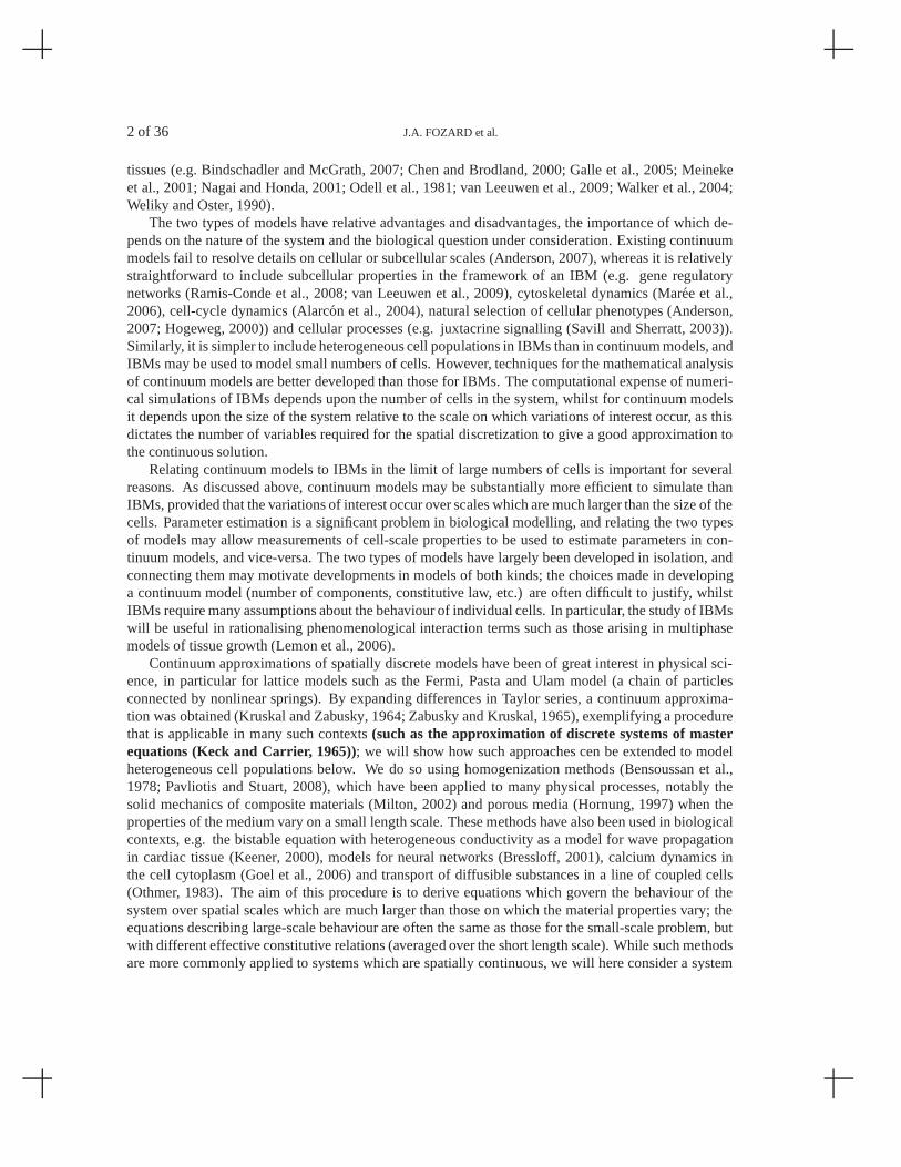
x0 x1 x2 xN

l3/2

a1/2 a3/2 aN−1/2

xN−1

FIG. 1. Variables and geometry for the one-dimensional vertex-based model.

The IBM will first be described in some detail in Section 2, where we discuss the underlyingmechanical framework. As in the CPM, the motion is driven by afree energy or Hamiltonian, butunlike the CPM, explicit consideration is made of dissipative forces. The approximation of thisIBM by a continuum model in the limit of a large number of cells is the subject of Section 3. Wederive a continuum approximation when the cell parameters differ slowly between cells throughreplacing finite differences in the IBM by derivatives in a relatively straightforward fashion. Wealso consider cells with heterogeneous parameters, for which continuum approximations are ob-tained using a multiple-scales approach. These are expressed in spatial variables in Section 4,permitting comparison with existing models; the continuummodels derived from the IBM con-tain convective derivatives which are not usually includedin models of this type. In order toassess the accuracy of these approximations, and to illustrate the behaviour of both the IBM andthe continuum approximation, we use our model framework to study an aggregate that consists ofexpanding cells in Section 5, making a brief comparison between the behaviour of this IBM andsome of the observations from wound-healing experiments inSection 5.5.

2. One-dimensional discrete model

We now give a detailed description of the one-dimensional IBM which is the subject of this paper.

2.1 Geometrical representation

We assume that each cell occupies a bounded interval; the cells adhere to each other and are unableto exchange positions with their neighbours. ForN touching cells arranged along a line, we denotethe positions of theN + 1 vertices byx0,x1, . . . ,xN, and the vertex velocities byun = dxn/dt; the cellsoccupy the intervals(x0,x1),(x1,x2), . . . ,(xN−1,xN), as illustrated in Figure 1. Quantities associatedwith the cell lying betweenxn andxn+1 are labelled with the subscriptn+ 1

2 (n = 0, . . . ,N− 1). Thephysical length of the cell by is given byln+1/2 ≡ xn+1−xn, so that

dln+1/2

dt= un+1−un, n = 0, . . . ,N−1. (2.1)

The notationx = (x0, . . . ,xN)T andu = (u0, . . . ,uN)T will sometimes be used for brevity. The dependentvariables of the system will comprise the vertex positions,x (or as the IBM will be invariant undertranslation, the cell lengths,ln+1/2), and the “target” (or “natural”) lengths of the cells,an+1/2, n =0, . . . ,N−1; the latter will increase at a rate which possibly depends on the properties and environmentalconditions of the cells.


2.2 Energy gradient formulation

As with many IBMs, such as theCPM (Graner and Glazier, 1992), vertex-based models (Nagai andHonda, 2001) or the one-dimensional model of Childress and Percus (1981), we will consider the evo-lution of the system as being driven by the decrease in anotional mechanical free energyH(x); weassume thatH depends only on the vertex positions, as their speeds (and hence the corresponding kineticenergies) are small.This provides a convenient framework through which to derive force balanceson individual vertices (boundaries between cells), although of courseH does not explicitly incorpo-rate the the constant turnover of chemical energy in cell maintenance and biochemical processes.However, mechanical energy will be generated by the cells through growth using chemical sourcesof energy; this will be included in the model later through parametric changes of some variables.Growth in the CPM is often handled in a similar manner (Glazier et al., 2007). This energy isdissipated through various mechanisms, such as viscous forces in the cell cytoplasm and cytoskeleton,and the breaking of cell-cell (cadherin) and cell-substrate (integrin) adhesions. The net rate of energydissipation is given byΦ(x,u), which we require to be non-negative, vanishing only whenu = 0. Therate of change of energy is given as a function ofu by

dHdt

= u ·∇xH(x),

where∇x ≡ (∂/∂x0,∂/∂x1, . . . ,∂/∂xN)T . Following Childress and Percus (1981), we assume that thesystem evolves such thatH(x) decreases most rapidly, under the constraint

Φ(x,u) = −u ·∇xH(x), (2.2)

on the velocityu, which is that the rate of change of energy balances the dissipation rate. The velocityu which minimises dH/dt, subject to (2.2), satisfies

∇xH(x)+ η∇uΦ(x,u) = 0, (2.3)

whereη is a Lagrange multiplier enforcing (2.2) and∇u ≡ (∂/∂u0,∂/∂u1, . . . ,∂/∂uN)T . We takeΦ tobe a quadratic form in the vertex velocities,

Φ(x,u) = uTD(x)u, (2.4)

(which is expected to be the case when the velocities are small, the resulting drag forces being linearfunctions of the vertex velocities) withD a symmetric matrix, in which case∇uΦ(x,u) = 2D(x)u.Taking the dot product of (2.3) withu, and subtracting (2.2), we find thatη = 1

2.The potential and dissipation functions can be considered as exerting generalized forces on the

vertices. The forcesF = (F0,F1, . . . ,FN)T acting as a result of the potential are defined as

F ≡−∇xH(x). (2.5)

We term such forces “static”, as they are independent of the vertex velocities. The damping forces,D = (D0,D1, . . . ,DN)T , generated by the dissipative processes are given (from (2.4)) by

D ≡−η∇uΦ(x,u) = −D(x)u.

With this notation (2.3) becomes

F+D = 0, (2.6)


which can be thought of as force balances on the vertices. In the specific model developed below, thefree energy and dissipation rate will both consist of a sum ofcontributions from individual cells, whichdepend only on the local properties and parameters of the cell. Each cell will exert static and drag forceson its end vertices, and so interacts directly only with its immediate neighbours.

2.2.1 The energy function Many types of cells will adhere to and spread out upon a surface (assumingthat the surface properties permit cell adhesion). This is acomplicated process, involving a balancebetween extensional forces generated by the cell (through the extension of pseudopodia and adhesion tothe substrate) and contractile forces actively generated by the cytoskeleton and as a result of its elasticity(Reinhart-King et al., 2005). Here we make the simple assumption that it is energetically favourable foreach cell,if isolated from its environment (but still adherent to a substrate), to attain its target length,an+1/2 (cf. the equilibrium area in the two-dimensional vertex-based model of Nagai and Honda (2001)).This length performs the same role in the resulting model as the length of a cell in the zero-stressstate for mathematical theories of tissue growth (Rodriguez et al., 1994).A similar energy term isincluded in the CPM (Graner and Glazier, 1992) in order to enforce cell incompressibility. In some two-dimensional models for epithelial cells (Chen and Brodland, 2000; Hilgenfeldt et al., 2008), the cellsare treated as having a fixed area in the plane of interest; in these models there is also a contribution tothe energy from the cell perimeter, as a result of the elasticproperties of the cortical cytoskeleton.

The energyH(x) will be taken to be a sum of contributions from each of the cells (depending onlyon local quantities), namely

H =N−1

∑n=0

C(ln+1/2,an+1/2;λn+1/2),

for some functionC(l ,a;λ ), whereλn+1/2 parametrises the mechanical properties of then-th cell (herethe cell elasticity and substrate adhesion). From (2.5), the static forces are then given by

Fn = pn−1/2− pn+1/2, n = 0, . . . ,N, (2.7)

where the cell “pressures”pn+1/2 are defined by

pn+1/2 ≡−∂C∂ l

(ln+1/2,an+1/2;λn+1/2), n = 0, . . . ,N−1.

Whilst thepn+1/2 are introduced primarily for notational convenience, theycorrespond to the forces (perunit length in the transverse direction) that would be exerted by the cells upon their neighbours (normalto the interface between cells), were the vertices stationary. We have not yet definedp−1/2 andpN+1/2;these depend on the external forces acting on the end vertices.

One simple model for the energy of the cells, equivalent to a system of linear springs between thevertices, is given by

C(l ,a;λ ) =λ2

(a− l)2 , pn+1/2 = λn+1/2(an+1/2− ln+1/2), n = 0, . . . ,N−1, (2.8)

whereλn+1/2 > 0, sopn+1/2 > 0 whenever a cell is under compression (an+1/2 > ln+1/2). This linearmodel is likely to be reasonable for small deformations; however it is not appropriate for situationswhere cells are highly compressed, when the pressure may exceedλn+1/2an+1/2.


2.2.2 The energy dissipation rateIn some works (e.g. Nagai and Honda, 2001), particularly wherethe equilibrium configurations are of primary concern, the dissipation rate is taken to beΦ = µuTu/2,with µ > 0, the corresponding drag forcesD = −µu being proportional to the speed of the vertices. Inthis paper, we will consider a more general model. We assume that

Φ =N−1

∑n=0

G(un,un+1, ln+1/2;µn+1/2,δn+1/2),

whereµn+1/2 > 0 parametrises the substrate drag of then-th cell andδn+1/2 > 0 parametrises its internalviscosity. The viscosity of a cell refers to the resistance of a cell to dynamic changes in shapethrough viscous dissipation in the cell cytoplasm and cytoskeleton.We model the energy dissipationof each cell as taking the formG = Gs+Gv, whereGs is the energy dissipated by drag between the celland substrate andGv is that dissipated by the internal viscosity of the cell. Thecorresponding drag forceon the vertexxn is Dn = Ds

n +Dvn, where

Ds,vn = −

12

∂∂un

(

min(n,N)

∑m=max(n−1,0)

Gs,v(um,um+1, lm+1/2;µm+1/2,δm+1/2)

)

.

The substrate exerts a drag on every point on the basal surface of the cell, the force per unit lengthbeing assumed proportional to the velocity, given by linearly interpolating the vertex velocities acrossthe base of the cell. The associated energy dissipation is then

Gs(un,un+1, ln+1/2;µn+1/2) = µn+1/2

∫ xn+1

xn

u2 dx

≃ µn+1/2

∫ ln+1/2

0

(

un(ln+1/2−y)+un+1y

ln+1/2

)2

dy

= 13µn+1/2ln+1/2

(

u2n +unun+1 +u2

n+1

)

.

Summing the contributions from all cells, the drag forces are given by

Dsn = −

µn−1/2ln−1/2(un−1+2un)

6−

µn+1/2ln+1/2(2un +un+1)

6, n = 0, . . . ,N. (2.9)

This formula holds for the end vertices (n = 0 andn = N) if we defineµ−1/2 = 0, µN+1/2 = 0.In reality, the cells form a large number of dynamic adhesions with the substrate and actively exert

forces upon it; in monolayers of proliferating cells these forces have been found to be mostly localizedat the boundaries between cells (du Roure et al., 2005). Experiments on wound healing in confluentmonolayers of cells (Farooqui and Fenteany, 2005) have indicated that, whilst the cells generally remainadherent to each other at their apical (top) end, the individual cells extend lamellipodia at their base andactively crawl on the substrate, rather than being pulled orpushed along by their neighbours. However,we neglect such details here, and assume that the cells “slide” across the substrate.

The cells also dissipate energy as a result of their internalviscosity; this is modelled using

Gv(un,un+1, ln+1/2;δn+1/2) = δn+1/2(un+1−un)2 (2.10)

for each cell, giving additional contributions of

Dvn = δn+1/2(un+1−un)− δn−1/2(un−un−1), n = 0, . . . ,N, (2.11)


to the drag forces acting on each vertex (as would be generated by dashpots connecting the vertices ofthe cells). Expression (2.11) is valid for alln if we takeδ−1/2 = δN+1/2 = 0. An alternative approachof Childress and Percus (1981) is to consider the cells as being filled with a fluid of viscosityηn+1/2,and to assume that each cell occupies a rectangle of fixed areaAn+1/2 in the cross section normal to thesubstrate. Further assuming that the extensional flow interpolates the velocities of the boundaries gives

Gv∗ = 4ηn+1/2An+1/2(un+1−un)2/l2n+1/2. (2.12)

We will not use this expression directly, but instead apply it later to estimate the typical size of theδn+1/2; if we fix ln+1/2 in (2.12) to be a typical cell length then it becomes of the same form as (2.10).

Using (2.7), (2.9) and (2.11), the force balance equation (2.6) becomes, forn = 0, . . . ,N,

µn−1/2ln−1/2(un−1+2un)

6+

µn+1/2ln+1/2(2un +un+1)

6−δn+1/2(un+1−un)+ δn−1/2(un−un−1) = pn−1/2− pn+1/2. (2.13)

2.3 Cell elongation

As indicated in Section 2.2,cellular metabolic processes do not fit naturally into the energy-gradientframework, and will instead be modelled separately with additional equations and rules. To include cellelongation or flattening (growth without cell division), wewill assume that the target lengths of the cellssatisfy

dan+1/2

dt= Γ (ln+1/2, pn+1/2,an+1/2;γn+1/2), n = 0, . . . ,N−1, (2.14)

whereγn+1/2 parametrises the growth-related properties (elongation rate) of then-th cell. As a simplemodel, we take

Γ (l , p,a;γ) = γ, (2.15)

so the target length of thenth cell increases at the constant rateγn+1/2; however, in comparisons withother models is it useful to consider other forms for the growth rate. We expect that cell elongation will,in general, be accompanied by cell division, but this process will be deferred to a later paper.

2.4 Overview of model

In summary, our IBM comprises the equations (2.1), (2.8) and(2.14), which hold for each cell (n =0, . . . ,N−1), and the force-balance equations (2.13), which hold for each vertex (n = 0, . . . ,N).

This differential-algebraic system contains a large number of subscripted quantities: the cell targetlengths,an+1/2, and actual lengths,ln+1/2, are differential variables (i.e. time derivatives appearexplic-itly) whilst the cell pressures,pn+1/2, and vertex velocities,un, are algebraic variables (time derivativesdo not appear explicitly). The remaining quantitiesµn+1/2, δn+1/2, λn+1/2 andγn+1/2 are non-negativeparameters, which will all be assumed to be constant.

2.5 Non-dimensionalisation and parameter estimation

We scale the cell parameters with typical values (denoted byasterisks)

µn+1/2 = µ∗µn+1/2, λn+1/2 = λ ∗λn+1/2, δn+1/2 = δ ∗δn+1/2, γn+1/2 = γ∗γn+1/2,


where we retain the possibility that properties may vary between cells. We scale the variables accordingto

an+1/2 = a∗an+1/2, ln+1/2 = a∗ ln+1/2, pn+1/2 = λ ∗a∗ pn+1/2, un = (λ ∗/µ∗)un,

t = (µ∗a∗/λ ∗)t,

and the growth function byΓ = Γ ∗Γ ,

whereΓ ∗ is a typical value ofΓ , anda∗ is the typical length of a cell. With the growth law (2.15) oneof Γ ∗ andγ∗ is redundant, in which case we take them to be equal.

We will use only dimensionless quantities in the remainder of this paper and henceforth omit thehats from the dimensionless variables. The system of equations then becomes

µn−1/2ln−1/2(un−1 +2un)

6+

µn+1/2ln+1/2(2un +un+1)

6−Vδn+1/2(un+1−un)+Vδn−1/2(un−un−1) = pn−1/2− pn+1/2, (2.16a)

for n = 0, . . . ,N, and

pn+1/2 = λn+1/2(an+1/2− ln+1/2), (2.16b)

dln+1/2

dt= un+1−un, (2.16c)

dan+1/2

dt= αΓ (ln+1/2, pn+1/2,an+1/2;γn+1/2), (2.16d)

for n = 0, . . . ,N−1, whereV = δ ∗/µ∗a∗, α = Γ ∗µ∗/λ ∗, (2.17)

are dimensionless parameters. HereV is the ratio of the drag due to the viscosity of the cells to that dueto the substrate, andα is the ratio of the cell elongation rate (Γ ∗/a∗) to the substrate-drag relaxationrate (λ ∗/µ∗a∗). The equations for the end vertices (n = 0,N) are that

µ1/2l1/2(2u0+u1)

6−Vδ1/2(u1−u0) = −p1/2, (2.18a)

µN−1/2lN−1/2(uN−1 +2uN)

6+VδN−1/2(uN −uN−1) = pN−1/2. (2.18b)

Representative parameter values are listed in Table 1. Mi etal. (2007) proposed a one-dimensionalcontinuum model for the healing of a wound in a monolayer of IEC-6 cells (intestinal epithelial cells);they considered a layer of cells with linear elasticity and cell-substrate drag which was pulled along bytraction forces generated by cells at the free edge. Estimating the traction forces using measurements ofPrass et al. (2006) of the force required to stall a migratingcell, and fitting the results of their model tothe experimental data of Cetin et al. (2007), gave estimatesof parameters which are equivalent toµ andλ in our model.

The model of Mi et al. (2007) did not include the effects of cell viscosity. We estimateδ ∗ using(2.12), and the approximate valueη ≃ 104Pas for the cell viscosity (Thoumine and Ott, 1997), fromwhich we have

δ ∗ =4ηh∗

a∗≃ 2×104Pas≃ 7Pah= 7×10−3hnN/µm2. (2.19)


Parameter Definition Value Sourcea∗ Cell target length 10µmh∗ Average cell height 6µmµ∗ Cell-substrate drag constant 0.01nNh/µm3 (Mi et al., 2007)λ ∗ Cell elastic constant 0.4nN/µm2 (Mi et al., 2007)δ ∗ Cell viscosity constant 7×10−3hnN/µm2 (2.19)Γ ∗ Cell growth rate 0.07µm/h (2.20)N Number of cells 10–40 (Poujade et al., 2007)

Table 1. Parameter estimates for epithelial cells

Before reaching confluence, IEC-6 cells have been observed to double in number every 20h (Quaroniet al., 1979). However, the growth rate may be significantly smaller within a monolayer because ofcontact inhibition; Corkins et al. (1999) suggested a doubling time ofTd ≃ 72h. If we assume that thetarget length of a cell must increase from a sizea∗/2 to a sizea∗ in this period, we obtain the estimate

Γ ∗ =a∗

2Td≃ 0.07µm/h. (2.20)

With these estimates, we find that the timescale for the dimensionless variables isµ∗a∗/λ ∗ ≃ 0.25h,and the dimensionless parameters describing the evolutionof individual cells are approximately

α ≃ 0.002, V ≃ 0.07, (2.21)

although we expect there to be significant deviations from these values for different cell types and whenindividual cells are exposed to different environmental signals.

3. Continuum approximations

The approximation of the IBM (2.16) by continuum models in the large cell-number limit is the focus ofthis paper. We first examine the case when the cell parametersvary slowly with respect to the cell indexin Section 3.1, introducing appropriate scalings for the cell variables and parameters, and replacing thefinite differences in the IBM by partial derivatives. In order to study this approximation in more detail,we compare the dispersion relationship for the continuum model with that for the IBM in Section 3.2.

To examine the case when cell parameters vary substantiallybetween neighbouring cells, we con-sider cell properties which are periodic in the cell index inSection 3.3. When the cell viscosity is small,the cell pressures and vertex velocities vary slowly with respect to the index, and satisfy the same systemof equations as for cells with properties that vary slowly inspace. However, when the cells have signifi-cant viscosity, we find that the pressures of neighbouring cells differ substantially, with the relationshipbetween the mean cell pressure and lengths depending upon the history of the cell lengths.

3.1 Slowly-varying approximation

The IBM (2.16) has a similar form to a (semi-discrete, or method of lines) finite-difference methodfor a particular system of partial differential equations.Such methods are usually considered in thelimit of vanishing mesh size, in which case the solution of the discrete equations generally convergesto the solution of the continuous equations. Here, the mesh size for the discrete equations is instead


fixed. If variations in cellular variables occur over large numbers of cells, then the derivatives of thecorresponding continuous functions are small, and so the (truncation) errors made in the approximationare also small; provided this slowly-varying condition holds, the continuum system will be a goodapproximation to the discrete model.

The physical quantities associated with each cell (pressure, target length, etc.) are defined only ata finite set of points for the IBM. For a given quantityφn+1/2 we may extend the initial data (e.g. byband-limited interpolation (Trefethen, 2000)) to a smoothfunctionφ(ν,t) (we useν, rather thann, todenote the cell label in the continuous case) forν ∈ [0,N], and we require that

φn+1/2 = φ(n+ 12,0), n = 0, . . . ,N−1.

This will serve as initial data for the system of partial differential equations (3.2), to be described shortly;for t > 0 we expect that

φn+1/2 ≃ φ(n+ 12,t), n = 0, . . . ,N−1.

We may similarly extend the initial data for the vertex positions to a smooth functionx(ν,t) on [0,N],although we now require thatxn = x(n,0), n = 0, . . . ,N, and for t > 0 we have the approximationxn ≃ x(n,t), n = 0, . . . ,N. The continuous velocityu(ν,t) is then defined byu(ν,t) = ∂x/∂ t, and wehave thatun ≃ u(n,t), n = 0, . . . ,N for t > 0. We then expand alln-dependent quantities using theirTaylor series, in (2.16a) aboutn, and in (2.16c) aboutn+ 1

2, as this minimises the asymptotic order ofthe error in the approximation. Assuming that all quantities are slowly-varying inν, with variationstypically occurring overN ≫ 1 cells, we rescale

ν = Nν , x = Nx, u = u/N, t = N2t, V = N2V, α = α/N2, p = p (3.1)

(these scalings ofV andα constitute a distinguished limit). To leading order asN → ∞ (in effect, retain-ing only the lowest derivatives that do not cancel in the Taylor expansions), (2.16) gives the followingsystem of equations:

µ l u− V∂

∂ ν

(

δ∂ u∂ ν

)

= −∂ p∂ ν

, (3.2a)

p = λ (a− l), (3.2b)

∂ l∂ t

=∂ u∂ ν

, (3.2c)

∂a∂ t

= αΓ (a, l , p,γ). (3.2d)

The terms omitted from these expansions are ofO(N−2). We discuss the physical interpretation of (3.2)in Section 4.1, where we also consider these equations in Eulerian (spatial) rather than Lagrangian (cell-based) coordinates. The appropriate boundary conditions are given by the Taylor expansions of (2.18);with the current scalings these become

p = Vδ∂ u∂ ν

at ν = 0,1, (3.3)

where the omitted terms are againO(N−2) provided that ˜u and p satisfy (3.2a).


The dimensionless parametersα andV for this rescaled system depend not only on the propertiesof the individual cells, but also the number of cells present, which will lie in the rangeN = 10 toN = 1000 for applications of interest here;in the wound healing experiments of Poujade et al. (2007)the the system is100to 400µm (roughly 10 to 40 cell diameters) across in the direction of interest.Assuming that the properties of individual cells are independent of monolayer size, we haveα = 0.2andV = 7× 10−4 for N = 10, whilst α = 2000 andV = 7× 10−8 for N = 1000. We note that withthese estimatesV is small compared with 1/N, which is the small parameter used in our continuumapproximations. However, we retain the viscous terms in thecontinuum approximations in order for ourmodel to be more generally applicable.

The IBM can be identified with a particular finite-element discretization of the continuum approxi-mation (3.2), and (3.2) could also be derived directly from the energy-gradient formulation of the IBM;both these matters are discussed in more detail in Appendix A. From (A.1), the free energyH = H/Nand dissipation rateΦ = NΦ associated with the continuum approximation are given by

H =

∫ 1

0

p2

2λdν, Φ =

∫ 1

0

{

µ l u2 + Vδ(

∂ u∂ ν

)2}

dν . (3.4)

3.2 Dispersion relationship for the IBM and the slowly-varyingcontinuum approximation

In order to investigate how the scale on which cell properties (e.g. pressure, length) vary affects thevalidity of the continuum approximation, and to illustratethe properties of both models, we examineand compare the dispersion relationships for the IBM (2.16)and the continuum approximation (3.2).In the absence of cell elongation,pn+1/2 = 0 for all n is the only steady state of the IBM; asH(x) isnon-increasingin this casethe trivial solution is stable.

We expect that short-wavelength modes will be poorly approximated as the derivatives of the so-lution, and hence the truncation errors, will not be small; as this is a local effect we will (just in thissection) consider an infinite line of cells. With uniform cell parameters (i.e.an+1/2 = µn+1/2 = λn+1/2 =δn+1/2 = 1 for all n), the IBM (2.16) linearized about the steady-state can be written as

16

(

dpn−1/2

dt+4

dpn+1/2

dt+

dpn+3/2

dt

)

−V

(

dpn−1/2

dt−2

dpn+1/2

dt+

dpn+3/2

dt

)

= pn+3/2−2pn+1/2+ pn−1/2

for all n. For modes of the formpn+1/2 = ℜ{

Ak(t)eikn}

(where admissible values ofk lie in the range0 6 k 6 2π : if k > 2π then the mode is identical to that with wavenumberkmod2π , a phenomenonknown as aliasing, see e.g. Trefethen (2000)) we have that the decay rate of the amplitude,dIBM, isgiven by

dIBM = −1Ak

dAk

dt=

12sin2 k2

(

1+2cos2 k2

)

+12V sin2 k2

.

(AsAk(t) remains real if the initial valueAk(0) is real, we may further restrict consideration to wavenum-bers in the range 0< k < π , because cos((2π −k)n) = cos(kn) for all integern.)

Linearizing the continuum approximation (3.2) about the steady statep = 0 yields the pseudo-parabolic equation

(

1−V∂ 2

∂ν2

)

∂ p∂ t

=∂ 2p∂ν2 .


Equations of this type arise in the study of second-order fluids (Ting, 1963) and in the flow of liquidthrough fissured rock (Barenblatt et al., 1960). For modes ofthe formp= ℜ

{

Ak(t)eikν}, the decay rateof the amplitude is

dC = −1Ak

dAk

dt=

k2

1+Vk2 .

For the IBM, the decay ratedIBM increases from 0 fork = 0 to a maximum value of 1/(V + 1/12) fork = π ; for the continuum approximation,dC increases from 0 fork = 0 to 1/V ask → ∞. In the limitk→ 0, which corresponds to our slowly-varying assumption, we have that

dIBM ∼ k2 +( 112−V)k4 +O(k6), dC ∼ k2

−Vk4 +O(k6);

these decay rates agree to leading order, and so long-wavelength modes are well approximated. ForV ≪ 1, short-wavelength modes (varying over finite numbers of cells), which are poorly approximatedby the continuum approximation, decay significantly more rapidly than those that vary on the scale ofthe whole aggregate (for whichk = O(N−1)). WhenV = V/N2 = O(1), modes which vary over a finitenumber of cells and over the whole aggregate decay at comparable rates.

3.3 Heterogeneous cell parameters

The approximation of Section 3.1 is valid only if the cell variables and parameters vary slowly withrespect to the cell index. However, we are also interested incases for which there is substantial variationin parameters between adjacent cells. In this case, we adopta multiple-scales approach, allowing allvariables to depend on both the discrete index,n, and the large length-scale variable,ν. Throughtreating these as independent variables, expanding all dependent quantities in inverse powers ofN, andimposing solvability conditions at each order, a system of partial differential equations for the dependentvariables is obtained. The analysis is presented in more detail in Appendix B, and we summarise theresults below. In order for the method used to be well-grounded, we restrict attention to situations inwhich the cell properties are periodic in the cell-indexn+ 1/2, with periodM = O(1)—this allows usto pursue a multiple-scales analysis that is traditional inperiodic homogenization. However, we discussthe application of these continuum models to problems with less well-structured cell properties. We alsoonly consider the case where the growth rate is constant for each cell (Γ ≡ γ).

WhenV = 0, we find in Appendix B.1 that the cell pressures,pn+1/2, and vertex velocities,un+1/2,at leading order depend on the index only through the large-scale variableν . Provided thatµn+1/2 isnot correlated with any of the other parameters (i.e. that the average of the product of the two quantitiesis equal to the product of the averages), we recover (3.2) forthe leading-order cell pressures, vertexvelocities and mean cell lengths, but with all parameters replaced by their average values over a period(which we denote by an overline), except forλn+1/2 for which the appropriate average is the harmonic

mean 1/(1/λn+1/2). The drag forces and growth rates for a group of cells combinelinearly, whichexplains the use of the arithmetic mean forµn+1/2 andγn+1/2. That the appropriate average for thestiffnessλn+1/2 is the harmonic mean can be understood by considering a groupof compressed cells atuniform pressure: the length of each cell will be less than its target length by an amount proportional to1/λn+1/2, and so the least stiff cells are the most compressed. The boundary conditions (3.3) again holdin this case (to leading order),as do the expressions (3.4), but with all parameters replaced by theirappropriate averages and the cell lengths replaced by theirmean values.


The viscous case (V = O(1)) is examined in Appendix B.2. Whilst the leading-order vertex veloci-ties again vary slowly with respect to the discrete index, the cell pressures are found to differ substan-tially between neighbouring cells. The mean cell lengthsl(ν , t), the mean target lengths ¯a(ν, t) and thevertex velocities, ˜u(ν,t), satisfy (to leading order)

µ l u−∂

∂ ν

(

κ∂ u∂ ν

)

= −∂

∂ ν

(

κ(

p

Vδ

)

)

, (3.5a)

∂ l∂ t

=∂ u∂ ν

, (3.5b)

∂ a∂ t

= α γ, (3.5c)

provided thatµn+1/2 is not correlated with any of the other cell parameters, where 1/κ =(

1/Vδ)

.However, the relationship between the mean cell pressures and cell lengths cannot be directly obtainedfrom the average of (2.16b), as ˜pn+1/2 andln+1/2 are correlated withλn+1/2, δn+1/2 andγn+1/2. Instead,we must considerM additional equations

qm+1/2− Vδm+1/2

(

αγm+1/2−1

λm+1/2

∂ qm+1/2

∂ t

)

= κ

{

(

p

Vδ

)

−∂ u∂ ν

}

, (3.5d)

which govern the pressures ˜qm+1/2(ν, t), m= 0, . . . ,M−1 of each of the cells in the periodic unit. Theleft-hand side of (3.5d) is (an approximation to)pn+1/2−Vδdln+1/2/dt, which is the total force exertedby a cell on its neighbours; as the right-hand side of (3.5d) is independent ofm, we see that it is thisquantity which differs only slightly between adjacent cells, whilst the pressure may vary substantially.Note that the ˜qm+1/2 are functions of the continuous cell indexν and so (3.5d) consists ofM partialdifferential equations (of the same form as (3.5b)) that arecoupled to (3.5a)–(3.5c).

In (3.5a) and (3.5d), the average of the pressures is given by

(

p

Vδ

)

=1M

M−1

∑m=0

qm+1/2(ν, t)

Vδm+1/2. (3.5e)

The pressures ˜pn+1/2 of the cells in the IBM are related to the ˜qm+1/2 through

pn+1/2(t) ≃ qn(modM)+1/2

(

n+ 12

N, t

)

.

The boundary conditions for equations (3.5) are that

(

p

Vδ

)

=∂ u∂ ν

at ν = 0,1. (3.6)

Equations (3.5d) provide a relationship between cell pressures and lengths, and are equivalent to simu-lating an aggregate ofM cells at each pointν ∈ [0,1], where the cells have no cell-substrate drag, andthe end vertices move such that the aggregate is expanding ata rateM∂ u/∂ ν.

To illustrate the need for (3.5d)–(3.5e), we consider the behaviour of this problem with constantexpansion rate∂ u/∂ ν, in which case the cell pressures can be found to be linear functions of time in the


long-time limit. However, the cell pressures relax to this solution on anO(V) timescale, and so whent = O(1) andV = O(1) we cannot treat the problem as being in quasi-equilibrium.

The above results were derived under the assumption that thecell properties were periodic withrespect to the cell index, with this period being much smaller than the total number of cells. Whilst it isrelatively straightforward to extend this analysis to cellproperties which are locally periodic, but varyon a long length-scale, this seems to be an unrealistic modelfor a heterogeneous collection of cells.Nethertheless, we believe that the resulting continuum approximation is applicable to less regularlystructured cell properties; this belief is borne out by numerical experiments (reported below). WhenV = 0, we expect that the same equations will hold as in the periodic case, but with the average overa period (overbars) interpreted as a ‘local’ average over cells that are large in number but comprise asmall fraction of the cell population (e.g.O(N1/2)). WhenV = O(1), we expect that (3.5a)-(3.5c) willstill hold with the average over a period replaced by the local average. However, rather than solvingequations (3.5d) for the pressures of each of the cells in a period, we instead examine ˜q(ν, t;δ ,γ,λ ),which is the local distribution of the pressure as a functionof the cell parameters. This satisfies

q− Vδ(

αγ −1λ

∂ q∂ t

)

= κ

{

(

p

Vδ

)

−∂ u∂ ν

}

, (3.7)

the average (3.5e) being replaced by

(

p

Vδ

)

=

∫∫∫

W(δ ,λ ,γ)q(ν , t;δ ,λ ,γ)

Vδdδ dγ dλ , (3.8)

whereW(δ ,λ ,γ) is the local distribution of cell properties, the integral in (3.8) being over the supportof W. The equations (3.7)–(3.8) can be seen to reduce to (3.5d)–(3.5e) in the spatially periodic case.

4. Spatial form of the continuum approximations, and comparison with existing models

The continuum approximations are now written in terms of spatial variables. We start by discussingthe features of these equations and then compare them with existing continuum models of growingmulticellular tissues,paying particular attention to the slow-elongation limit.

4.1 Spatial form of the continuum approximations

The use of the (Lagrangian) cell indexν as an independent variable in the continuum model hinderscomparison with existing models. Instead, we transform theindependent variables from(ν,t) to (x,t),wherex(ν,t) is the physical (Eulerian) position of the vertex with indexν (corresponding toxn in thediscrete model). On the population scale, we writex = Nx, andx(ν, t) satisfies

(

∂ x∂ ν

)

t= l ,

(

∂ x∂ t

)

ν= u


(cf. dxn/dt = un for the discrete equations). In spatial variables, (3.2) becomes

µ u− V∂∂ x

(

δ l∂ u∂ x

)

= −∂ p∂ x

, (4.1a)

p = λ (a− l), (4.1b)

DlDt

= l∂ u∂ x

, (4.1c)

DaDt

= αΓ (a, l , p;γ), (4.1d)

where we have introduced the convective derivative

DDt

≡∂∂ t

+ u∂∂ x

.

Thus

DφDt

= 0, (4.1e)

for any propertyφ which is constant in time for a particular cell (e.g.λ , δ , γ, µ). These equations holdon xL < x < xR, where (3.3) becomes

p = Vδ l∂ u∂ x

at x = xL, xR, (4.2)

and the boundaries move with the local cell velocity ˜u, so dxL,R/dt = u(xL,R, t).We note that the transport of other cellular properties (such as protein concentrations) may be mod-

elled using equations similar to (4.1e); ifcn+1/2 is a cellular property satisfying dcn+1/2/dt = F(cn+1/2)(e.g. c could be the level of a protein with intracellular production rateF(c)), and which varies slowlywith the cell index, then the appropriate equation in spatial coordinates is

DcDt

= F(c).

The restriction that the cell properties vary slowly with the cell index is essential; a differentapproach would be needed when this is not the case (e.g. for cell-cycle models).

Using (4.1b)–(4.1d), we may rewrite (4.1c) as

αΓ − l∂ u∂ x

=1λ

DpDt

, (4.3)

from which we see that the convective derivative of the cell pressure is also contained in this model.Whilst this convective derivative appears in the continuummodel derived from an IBM by Childressand Percus (1981), or implicitly in models formulated in Lagrangian coordinates (e.g. Mi et al. (2007)),many other extant models neglect such contributions. Defining the cell density byρ = 1/l , (4.1c) isequivalent to

∂ρ∂ t

+∂∂ x

(ρ u) = 0,


corresponding to conservation of cell number.WhenV = 0, (4.1a) reduces to Darcy’s law (used to model the flow of a viscous fluid through a

porous medium); similar pressure-velocity relationshipshave been used in incompressible fluid modelsfor solid tumours (e.g. Greenspan, 1976), although the biological system considered here is a two-dimensional sheet of cells lying on a substrate rather than athree-dimensional spheroid. WhenV > 0,there is an additional term of Brinkmann-viscosity form corresponding to the extensional viscosity ofthe cells in (4.1a), and a similar term in the boundary condition (4.2).

We may apply the same transformation from cell-based to spatial variables for heterogeneous cellparameters, but for brevity we omit the resulting equationshere.

4.2 Comparison with other models in the slow-elongation limit

We now approximate (4.1) in the slow-elongation limitα ≪ 1 (with V = O(1) or smaller), which (fromthe estimates of Section 3.1) we expect to be appropriate forrelatively small numbers of cells; this limitmay also be appropriate for larger numbers of cells of a different type, or if there is significant inhibitionof growth within the layer. The appropriate timescale ist = O(1/α), as the cells grow by a finite amountover this long period. The cell pressures and vertex velocities should be of equal order to balance termsin (4.1a), and from (4.3) we see that ˜p = O(α) andu = O(α). We rescale using

p = α p, u = αu, t = t/α, (4.4)

in which case we have to leading orderl = a+O(α) and

µ u− V∂∂ x

(

δa∂ u∂ x

)

= −∂ p∂ x

, (4.5a)

a∂ u∂ x

= Γ , (4.5b)

DaDt

= Γ ,DφDt

= 0, φ = λ ,µ ,δ ,γ, (4.5c)

whereDDt

≡∂∂ t

+ u∂∂ x

,

with boundary conditions (4.2) at ˜x = xL andx = xR, the boundaries moving with the local cell velocityu; the convective derivative of the cell pressures on the right-hand side of (4.3) is small in this limit.Differentiating (4.5a) with respect to ˜x gives

Γa− V

∂∂ x

(

1µ

∂∂ x

(δΓ )

)

= −∂∂ x

(

1µ

∂ p∂ x

)

,

with the boundary conditions ˇp = VδΓ , x = xL, xR, which is an elliptic problem for the cell pressuresat each moment in time. This approximation will be valid fort = O(1); for small time there will betransient behaviour in which the solution evolves from the initial data to a quasi-equilibrium state.

If Γ ≡ γ lS(p) ≃ γaS(p) (so that the source term per unit length is a function of pressure alone), thesystem (4.5) becomes

γ{

S(p)− V∂∂ x

(

1µ

∂∂ x

(δaS(p))

)}

= −∂∂ x

(

1µ

∂ p∂ x

)

,∂ u∂ x

= γS(p),DaDt

= γaS(p),DφDt

= 0,


along with the boundary conditions ˇp = VδγaS(p) at x = xL, xR. WhenV = 0, this is similar in form tothe single-phase incompressible-fluid models developed byGreenspan (1976) to describe the growth ofa (three-dimensional) cellular aggregate. Many other models exist for solid tumours, some of which arereviewed by Araujo and McElwain (2002) and Roose et al. (2007). Sheets of cells have been less wellstudied using continuum models; along with those mentionedpreviously (Childress and Percus, 1981;Mi et al., 2007), there are also reaction-diffusion models (Sherratt and Murray, 1990), those which con-sider cells moving within an elastic tissue (Murray and Oster, 1984; Olsen et al., 1995; Tranquillo andMurray, 1992) (comprising a force balance equation for the whole tissue and conservation equations forcell densities), and models which treat an epithelium as a growing elastic beam (Edwards and Chapman,2007).

5. Expansion of a cellular island

We now consider the expansion of an island of cells caused by an increase in their target lengths (cellexpansion). We examine the validity of the continuum approximations as the number of cells in the IBMvaries and discuss the effects of cell heterogeneity. We also consider the behaviour of the models in thesmall-growth-rate and long-time limits. Rather than give an exhaustive description of the behaviour ofthe system in all possible parameter regimes, we instead illustrate its behaviour for a few choices ofparameter values.

5.1 Parameters, initial data and continuum approximations

In the simulations, the growth rate (rate of increase of the target length,a) will be taken to be constant intime for each cell (Γ ≡ γ). For uniform cell parameters, through an appropriate choice of scales in ournon-dimensionalisation, we setλn+1/2 = δn+1/2 = µn+1/2 = γn+1/2 = 1 and take the initial target lengthsto bean+1/2 = 1 att = 0 for all cells, so thatan+1/2(t) = 1+ α t from (3.2d). The initial positions of thevertices are taken to be

xn = n− N2 , n = 0, . . . ,N,

so all cells are uncompressed (pN+1/2 = 0) and have unit length (ln+1/2 = 1), the aggregate occupyingthe region−N/2< x< N/2. In the heterogeneous case, the cell parameters and initial target lengths aretaken to beδn+1/2 = µn+1/2 = 1 andan+1/2(0) = 1 for all cells, butλn+1/2 andγn+1/2 are periodic inthe cell index (with period 4) as listed in Table 2. The cell target lengths are thenan+1/2 = 1+ αγn+1/2t,with the mean being ¯a = 1+ α t. The initial vertex positions,xn, are again chosen such that all cellshave zero pressure, the aggregate occupying the region−N/2 < x < N/2. Solutions to these discreteproblems depend upon timet, the dimensionless parametersα andV, and the number of cellsN.

For both slowly-varying and heterogeneous cell parameters(in the latter case, forV ≪ 1), the celllengths can be eliminated from the continuum approximation, giving

(1+ α t − p)u− V∂ 2u∂ ν2 = −

∂ p∂ ν

, α −∂ p∂ t

=∂ u∂ ν

, (5.1)

on 0< ν < 1, with boundary conditions

p = V∂ u∂ ν

at ν = 0,1, (5.2)

and initial data ˜p = 0 at t = 0. For heterogeneous cell parameters with significant cell viscosity (V =O(1)), the cell viscosities are taken to be uniform (δn+1/2 = 1 for all n) for simplicity; the continuum


n 4s 4s+1 4s+2 4s+3γn+1/2 3/2 1/2 3/2 1/2λn+1/2 2/3 2/3 2 2

Table 2. Cell parameter values used for the heterogeneous problems: δn+1/2 = µn+1/2 = 1 for all cells, whilst the cell elasticconstants,λn+1/2, and growth rates,γn+1/2, are as shown above for fors= 0, . . . ,(N−4)/4, with periodM = 4.

approximation (3.5) can be written as

(

1+ α t −

(

qm+1/2

λm+1/2

)

)

u− V∂ 2u∂ ν2 = −

∂ q∂ ν

, (5.3a)

1

V

(

qm+1/2− q)

− αγm+1/2 +1

λm+1/2

∂ qm+1/2

∂ t= −

∂ u∂ ν

, m= 0, . . . ,M−1, (5.3b)

on 0< ν < 1, with boundary conditions

q = V∂ u∂ ν

at ν = 0,1,

and the initial data ˜qm+1/2 = 0, m= 0, . . . ,M −1. Whilst we solve the problem (numerically) in cell-based variables, the transformation to spatial coordinates, x(ν, t), is given by the solution of∂ x/∂ t = uwith initial data x = ν − 1/2 at t = 0. The solution ˜p(ν , t), u(ν , t) and x(ν , t) (or qm+1/2(ν, t), m =

0, . . . ,M − 1, u(ν , t) and x(ν , t)) depends only onα andV. In general, we are unable to find an ex-plicit solution to the initial-boundary value problems(5.1) and (5.3), but instead approximate themnumerically using a semi-discrete Galerkin finite element method, as described in Appendix A.

5.2 Uniform cell parameters

We examine numerical simulations of the IBM (2.16)–(2.18) and the continuum model (5.1)–(5.2)in Figures 2 and 3, without and with cell viscosity, respectively. In both cases, we find that the totalsize of the aggregate and the maximum cell pressure increasewith time. In Figure 2, there is no cellviscosity (V = 0); the vertex velocities are approximately linear inν (or x), and the pressure profile isapproximately parabolic, driving the motion of the cells. The pressure is greatest in the centre of theaggregate, as the aggregate expands symmetrically about its centre. Figure 3 shows that, with viscosity(V = 1), the pressure profile is still approximately parabolic, but now contains a uniform componentthat increases with time and is needed to overcome the internal viscosity of the cells as they expand.The velocity profile is still approximately linear in the cell index ν, but the maximum cell speed nowincreases (noticeably) with time. Both with and without cell viscosity, we find that the differencesbetween the IBM and the continuum approximation att = 1 (and withα = 1) scale likeN−2. Evenfor N = 5 cells, the IBM and the continuum approximation are in closeagreement, with the maximumabsolute errors in ˜p andu (with α = 1 and att = 1) being approximately 4×10−3 and 1×10−4 withoutviscosity (V = 0), or 5×10−4 and 3×10−5 with cell viscosity (V = 1).

As discussed in Section 4.2, the continuum approximation simplifies to (4.5) in the limitα ≪ 1; inthis case it is appropriate to examine the solution in the rescaled variables ˇp, u andt, as defined by (4.4).


00.050.1

0.150.2

0.250.3

0.350.4

0.45

-1.5 -1 -0.5 0 0.5 1 1.5

p

x

t = 0.5t = 1t = 2

(a)

-0.5-0.4-0.3-0.2-0.1

00.10.20.30.40.5

-1.5 -1 -0.5 0 0.5 1 1.5

u

x

t = 0.5t = 1t = 2

(b)

00.050.1

0.150.2

0.250.3

0.350.4

0.45

0 0.2 0.4 0.6 0.8 1

p

ν

t = 0.5t = 1t = 2

(c)

-0.5-0.4-0.3-0.2-0.1

00.10.20.30.40.5

0 0.2 0.4 0.6 0.8 1

u

ν

t = 0.5t = 1t = 2

(d)

FIG. 2. Expansion of a homogeneous aggregate ofN = 20 cells without cell viscosity (V = 0), extending at a constant rate (Γ ≡ 1),and with expansion rate parameterα ≡ N2α = 1. Results are displayed in rescaled variables ˜x≡ x/N, ν ≡ ν/N, u≡ u/N, p≡ p,and the solutions are evaluated att ≡ t/N2 = 0.5,1,2. The markers show the pressures at the mid-points of the cells, pn+1/2, in (a),(c) and the velocities of the vertices, ˜un, in (b), (d) computed using the IBM (2.16)–(2.18), whilst the broken lines are numericalsimulations of the continuum approximation (5.1)–(5.2). Plots (a), (b) show the solution in terms of the spatial variable x, whilst(c), (d) show the solution in terms of the cell-index variable ν.

0.4

0.6

0.8

1

1.2

-1.5 -1 -0.5 0 0.5 1 1.5

p

x

t = 0.5t = 1t = 2

(a)

-0.5-0.4-0.3-0.2-0.1

00.10.20.30.40.5

-1.5 -1 -0.5 0 0.5 1 1.5

u

x

t = 0.5t = 1t = 2

(b)

0.4

0.6

0.8

1

1.2

0 0.2 0.4 0.6 0.8 1

p

ν

t = 0.5t = 1t = 2

(c)

-0.5-0.4-0.3-0.2-0.1

00.10.20.30.40.5

0 0.2 0.4 0.6 0.8 1

u

ν

t = 0.5t = 1t = 2

(d)

FIG. 3. Expansion of a homogeneous aggregate of cells; as in Figure 2 but with cell viscosity (V = 1).


0

0.05

0.1

0.15

0.2

0.25

0.3

0.35

0.4

-1 -0.5 0 0.5 1

p≡

p/α

x

α = 1α = 0.1

α = 0.01

(a)

-0.6

-0.4

-0.2

0

0.2

0.4

0.6

-1 -0.5 0 0.5 1

u≡

u/α

x

α = 1α = 0.1

α = 0.01

(b)

0.6

0.8

1

1.2

1.4

1.6

-1 -0.8 -0.6 -0.4 -0.2 0 0.2 0.4 0.6 0.8 1

p≡

p/α

x

α = 1α = 0.1

α = 0.01

(c)

-0.5-0.4-0.3-0.2-0.1

00.10.20.30.40.5

-1 -0.8 -0.6 -0.4 -0.2 0 0.2 0.4 0.6 0.8 1u≡

u/α

x

α = 1α = 0.1

α = 0.01

(d)

FIG. 4. Small growth-rate behaviour of the IBM and continuum approximation for an aggregate ofN = 20 cells, with varyingvalues ofα; the solutions are displayed in the rescaled variables ˜x≡ x/N and p≡ p/α ≡ p/N2α in (a), (c), oru≡ u/α ≡ u/Nαin (b), (d), all solutions being evaluated att ≡ α t ≡ αt = 1. Plots (a), (b) show the behaviour without cell viscosity (V = 0), whilst(c), (d) are with cell viscosity (V = 1). The broken lines show the solution of the continuum approximation (5.1)–(5.2) for eachvalue ofα , whilst the solid line is the approximation (5.4), valid in the limit α → 0.

The reduced system (4.5) has the exact solution

p =1+ t

2

{

14−

x2

(1+ t)2

}

+ V, u =x

1+ t, −

1+ t2

6 x 61+ t

2. (5.4)

We compare numerical simulations of the IBM, the continuum approximation (5.1)–(5.2), and (5.4) att = 1 in Figure 4, where we confirm that the models approach the solution (5.4) in the limitα → 0, bothwith and without cell viscosity.

5.3 Heterogeneous cell parameters

In this section, we consider cells with heterogeneous parameters, as listed in Table 2. Withoutcell viscosity (V = 0), the IBM and continuum approximation (5.1)–(5.2) can be seen in Figure 5 tobe in reasonable agreement, even when the number of cells is moderate (N = 8). The solution to thecontinuum approximation is symmetric about ˜x = 0, but the solution to the IBM is shifted to the left;this higher-order correction is a consequence of the asymmetry of the cell parameters in each period.

WhenV = O(1), the leading-order cell pressures depend on the discrete indexn, whilst the leading-order vertex velocities depend on the discrete index only through the large length-scale variableν . Thiscan be seen in Figure 6, where we examine the solution of the IBM at a single point in time: the cellpressures are oscillatory in space, whilst the vertex velocities differ only slightly between neighbouring


00.050.1

0.150.2

0.250.3

0.350.4

-1.5 -1 -0.5 0 0.5 1 1.5

p

x

t = 0.5t = 1t = 2

(a)

-0.5-0.4-0.3-0.2-0.1

00.10.20.30.40.5

-1.5 -1 -0.5 0 0.5 1 1.5

u

x

t = 0.5t = 1t = 2

(b)

FIG. 5. Expansion of an inviscid aggregate of (N = 8) cells; as in Figure 2 (a), (b), but with periodic cell properties as listed inTable 2.

00.20.40.60.8

11.21.41.61.8

-0.8 -0.6 -0.4 -0.2 0 0.2 0.4 0.6 0.8

p

x

t = 1(a)

-0.4

-0.3

-0.2

-0.1

0

0.1

0.2

0.3

0.4

-0.8 -0.6 -0.4 -0.2 0 0.2 0.4 0.6 0.8

u

x

t = 1

(b)

FIG. 6. Expansion of an aggregate of cells with periodic cell properties; as in Figure 5, but forN = 32 cells with viscosity (V = 1).The markers show the pressures at the mid-points of the cells(a) and the vertex velocities (b) in the IBM (2.16)–(2.18), evaluatedat t = 1. In (a), we plot the solutions ˜q1/2 (short dashes), ˜q1+1/2 (dash-dotted), ˜q2+1/2 (solid) and ˜q3+1/2 (long dashes) of the

continuum approximation (5.3), which are the pressures of the cells in each period ( ˜pn+1/2 ≃ qn(modM)+1/2((n+ 12)/N, t)); we

also plot a dotted line joining the pressures at the centres of the first six cells to emphasise the spatial oscillations.


00.050.1

0.150.2

0.250.3

0.350.4

-1.5 -1 -0.5 0 0.5 1 1.5

p

x

t = 0.5t = 1t = 2

(a)

-0.5-0.4-0.3-0.2-0.1

00.10.20.30.40.5

-1.5 -1 -0.5 0 0.5 1 1.5

u

x

t = 0.5t = 1t = 2

(b)

00.20.40.60.8

11.21.41.61.8

-0.8 -0.6 -0.4 -0.2 0 0.2 0.4 0.6 0.8

p

x

t = 1(c)

-0.4

-0.3

-0.2

-0.1

0

0.1

0.2

0.3

0.4

-0.8 -0.6 -0.4 -0.2 0 0.2 0.4 0.6 0.8u

x

t = 1

(d)

FIG. 7. Expansion of aggregates of (N = 32) cells with non-periodic heterogeneous cell properties; for (a), (b) without viscosity(V = 0 as in Figure 5), and for (c), (d), with cell viscosity (V = 1 as in Figure 6), but with the parameters in each period of 4 cellspermuted randomly.

vertices. This is compared with the simulations of (5.3), which yields approximations ˜qm+1/2, m =0, . . . ,M −1, to the pressures of theM = 4 cells in each period. Both with and without cell viscosity,the maximum absolute difference between the IBM and the continuum approximation is found to beO(N−1) for largeN. This error has a spatially oscillating component caused bylocal variation in cellularparameters, and a smooth component needed for the solution to satisfy the discrete boundary conditions(2.18).

To confirm our belief that the continuum approximation does not require periodicity of cell parame-ters, we examine the simple case in which the parameters of the cells are as in Table 2, but with the fourcells in each period permuted randomly.The cell parameter distribution W(δ ,λ ,µ) is the same asin the periodic case, namely

W(δ ,λ ,µ) =1M

M−1

∑m=0

d(δ − δm+1/2)d(λ −λm+1/2)d(µ − µm+1/2),

where d(·) denotes the delta function; (3.7) and (3.8) reduce to (3.5d)and (3.5e), respectively.Theresults of these simulations are shown in Figure 7, where thecontinuum approximation and IBM canagain be seen to be in reasonable agreement; for the simulations withV = 0 the error is noticeably largerthan in Figure 5, although we note that the number of cells (N = 8 cells, corresponding to two groupsof four cells) is not overly large.

The behaviour in the slow-growth-rate (α ≪ 1) limit is also of interest. In the absence of cellviscosity (V = 0), the leading-order behaviour is given by (5.4), just as for uniform cell parameters.When the cells have significant viscosity (V = O(1)), on rescaling ˜qm+1/2 = αqm+1/2 and all other


variables following (4.4), equations (5.3) become

u− V∂ 2u∂ ν2 = −

∂ q∂ ν

, (5.5a)

qm+1/2− q = V

(

γm+1/2−∂ u∂ ν

)

, m= 0, . . . ,M−1 (5.5b)

to leading order. Taking the average of (5.5b) over a period gives

∂ u∂ ν

= 1 (5.6)

(asγ = 1 here), so the pressures of the individual cells are relatedto the mean pressureq through

qm+1/2 = q+ V(γm+1/2−1), m= 0, . . . ,M−1, (5.7)

the local variations in cell pressure being caused by differences in growth rates, and so viscous forces.The solution to (5.5a) and (5.6) is given by (5.4) with ˇp replaced by the average cell pressureq. We notethat the continuum approximation greatly simplifies in thislimit, as (5.3b) has the explicit (approximate)solution (5.7).

5.4 Long-time behaviour

Finally, we briefly examine the long-time behaviour of solutions to (5.1). Posing the ansatz ˜p= α tP(ν),u = U(ν), x = α tX(ν), we have from (5.1) that

(1−P)U = −dPdν

, α(1−P) =dUdν

,dXdν

= 1−P, X(12) = 0,

to leading order int, with the boundary conditionsP = 0 at ν = 0,1, and the symmetry conditionX(1/2) = 0. This has solution

P = 1−B−αX2

2, U = αX, X =

√

2Bα

tan

(

√

Bα2

(

ν −12

)

)

, (5.8)

for some constantB determined by the boundary conditionsP = 0 at ν = 0 andν = 1: for α ≪ 1 wehaveB∼ 1− α/8; for α ≫ 1 it is found thatB∼ 2π2(1−4

√

2/α)/α. The cell viscosity,V, does notaffect the leading-order solution in this limit (provided that t ≫ V). We plot simulations of the IBMand the continuum approximation (5.1)–(5.2) in these similarity variables in Figure 8, where they canbe seen to approach (5.8) in the long-time limit. The simulations in Figure 8 are the same cases as thosein Figures 2 and 3, but evaluated at later time points.

For heterogeneous cell parameters, we find that the long-time behaviour is the same as with uniformcell parameters (the cell pressures being slowly-varying to leading order even forV = O(1)). However,the IBM can be observed numerically to break down in this limit; the maximum pressure grows likeα tP(1/2), whilst the maximum pressure which can be sustained by a cell(with the model (2.8) for thecell mechanical properties) isλn+1/2(1+ αγn+1/2t). As P(1/2) is an increasing function ofα, withP(1/2) = 0 for α = 0 andP(1/2) → 1 asα → ∞, the lengths of some cells become negative ifα issufficiently large (namely ifP(1/2) > min(γm+1/2λm+1/2); this is not the case in the simulations ofFigure 8).


0

0.02

0.04

0.06

0.08

0.1

0.12

0.14

0.16

-0.6 -0.4 -0.2 0 0.2 0.4 0.6

P≡

p/α

t

X ≡ x/α t

t = 10t = 20t = 40

(a)

-0.5-0.4-0.3-0.2-0.1

00.10.20.30.40.5

-0.6 -0.4 -0.2 0 0.2 0.4 0.6

U≡

u

X ≡ x/α t

t = 10t = 20t = 40

(b)

0

0.05

0.1

0.15

0.2

0.25

-0.5 -0.4 -0.3 -0.2 -0.1 0 0.1 0.2 0.3 0.4 0.5

P≡

p/α

t

X ≡ x/α t

t = 20t = 40t = 80

(c)

-0.5-0.4-0.3-0.2-0.1

00.10.20.30.40.5

-0.5 -0.4 -0.3 -0.2 -0.1 0 0.1 0.2 0.3 0.4 0.5U

≡u

X ≡ x/α t

t = 20t = 40t = 80

(d)

FIG. 8. Long-time behaviour for the expansion of an island of cells (with N = 20 cells andα = 1), plotted in the similarityvariablesP = p/α t , U = u andX = x/α t, with V = 0 in (a), (b) andV = 1 in (c), (d); the solid line is the asymptotic solution(5.8), where forα = 1 we have thatB≃ 0.893.

5.5 Wound-healing assays

The migration of cells can be investigated using ‘wound-healing’ assays, in which a confluent ep-ithelium is made to have a free edge, either by scratching thelayer with a razor blade or pipettecone, or by removing a stencil which previously confined the cells (Poujade et al., 2007). Some ep-ithelial cell lines (e.g MDCK cells) maintain cell-cell contacts and migrate collectively as a sheet, inwhich case the mean distance travelled by the free edge is a superlinear (approximately quadratic)function of time (Farooqui and Fenteany, 2005; Rosen and Misfeldt, 1980) (although the speed ofthe edge may level off after several days, as suggested by Rosen and Misfeldt (1980)). Whilst celldivision does occur in such an assay (Poujade et al., 2007), with the total number of cells increasinglinearly with time, similar results for the first 10 hours aft er wounding have been obtained withmitotically inhibited cells.

In Figure 9, we examine the velocity of the right-hand edge ofan island of N = 20 identicalcells, with expansion rate parameterα = 1 and a variety of values for the cell viscosity parameter,V. (The lines for V = 0 and V = 1 correspond to the simulations of Figures 2 and 3, respectively.)In all cases, the speed of the edge increases with time. In theabsence of cell viscosity (V = 0), thisacceleration is associated with the establishment of a parabolic pressure profile in the layer; forthe continuum approximation the speed of the edge is found tobe proportional to t1/2 for smalltime. Cell viscosity acts to further slow the development ofa pressure gradient in the aggregate,reducing the initial acceleration; the behaviour for small dimensionless time may partly explainthe roughly uniform acceleration observed in experiments.The velocity of the edge tends towardsa constant value for sufficiently large time (see (5.8)) as a consequence of the fixed number of cellsand the constant growth rates. The present model therefore provides a mechanistic description of


00.050.1

0.150.2

0.250.3

0.350.4

0.450.5

0 0.5 1 1.5 2u

t

V = 0V = 0.1

V = 0.25V = 1

FIG. 9. The velocity of the right hand-edge of an expanding island of cells (withN = 20 andα = 1), for a variety of differentvalues of the cell viscosity parameter,V. The results are displayed in the rescaled dimensionless variablesu≡ u/N andt ≡ t/N2.

the superlinear growth seen experimentally.

6. Discussion

In this paper, we have presented a simple one-dimensional IBM for a layer of adherent cells. Continuummodels which approximate its behaviour in the limit of largenumbers of cells were derived, both whenthe cell parameters vary slowly in space, and when they are heterogeneous (and periodic);most previousworks which derive a continuum model from an IBM assume that all cells are identical. In theformer case, we were able to replace finite differences in theIBM by partial derivatives in the resultingcontinuum model. In the latter case, we adopted a multiple-scales approach; when the cell viscositywas small (V ≪ 1), we found that the cell pressures and vertex velocities varied slowly in space. Thecontinuum approximation with heterogeneous parameters took the same form as in the slowly-varyingcase, but with all cell parameters replaced by their appropriate averages; for the cell stiffnessλn+1/2, this

was not the arithmetic meanλn+1/2, but rather the geometric mean 1/(1/λn+1/2). However, when thecells have significant viscosity (V = O(1)) and heterogeneous parameters, the pressures of neighbouringcells may differ substantially, and the relationship between mean cell lengths and pressures is found todepend upon the history of the solution; the local problem relaxes to a steadily expanding state on atimescale which is comparable to that on which the large-scale problem evolves. As a consequence,a group of cells (without cell-substrate adhesion) must be simulated at each point in space in order toobtain the effective constitutive relation.

The resulting continuum models (apart from that for the heterogeneous problem with cell viscosity)resemble existing incompressible fluid models for cell growth, but with the addition of Brinkmann-viscosity terms and convective derivatives of the cell pressures. From the parameter estimation in Sec-tion 2.5, it seems likely that the viscous terms are small, but the convective derivatives(often ignored incontinuum models of growing tissues, e.g. Greenspan (1976), Byrne and Chaplain (1996))may besignificant. The continuum models provide good approximations to the IBM, even for moderate (N = 5)numbers of cells. Furthermore, the continuum approximation facilitates the analysis of the system inthe slow-growth-rate and long-time limits.

The IBM considered here was intentionally simplistic, in order to illustrate the techniques involvedin the derivation of continuum approximations. As each cellis treated as a distinct entityin the IBMit is straightforward to include subcellular processes, for example regulatory networks modelled bysystems of ordinary differential equations,such as those controlling planar cell polarization (Klein


and Mlodzik, 2005). We reiterate that the continuum approximation of Section 4.1 is valid onlywhen the state of the cellular processes varies slowly between neighbouring cells; when this isnot the case, for example in patterning through juxtacrine signalling (Owen et al., 2000), or formodels of the cell cycle (Novak and Tyson, 2004), a more sophisticated approach is necessary. Themechanical model used for the cells could also be increased in complexity—in particular, the treatmentof cell-cell and cell-substrate adhesion could be made morephysically realistic.Active cell migrationcould also be included in this model by the addition of terms (the chemotactic potential) to the freeenergy of the cells (as discussed by Glazier et al. (2007) forthe CPM). However, the most significantprocess which is lacking in the current IBM is cell division.Cell division complicates the model, as thenumber of discrete entities in the system (and so the number of variables in the IBM) increases, requiringrelabelling of the cells in both the IBM and the continuum approximation (in cell-based coordinates).Furthermore, cells are unlikely to divide in synchrony, causing local variation in cell sizes and providingadditional motivation for our study of the IBM with heterogeneous cell parameters.

This IBM is a one-dimensional analogue of the two- or three-dimensional vertex-based models ofNagai and Honda (2001) and Chen and Brodland (2000); it is clearly desirable to extend the analysis ofthis paper to higher dimensions. However, this is significantly complicated by the fact that the neigh-bours of a given cell are not fixed, but may change through topological transitions (Weaire and Fortes,1994; Weaire and Rivier, 1984), leading to irreversible plastic deformations of the tissue.Preliminarystudies of a two-dimensional version of this model suggest that the cells on the outer surface of anaggregate may adopt a significantly different shape to thosein the interior. Such discrete effectsmay require consideration of a hybrid model, in which a continuum approximation in the interioris matched with a discrete solution valid near the edge.

In summary, when the number of cells in the IBM is large, we mayapproximate its behaviour witha continuum model. When the parameters of cells vary slowly in space, the approximation is valid if thecell pressures and vertex velocities vary spatially over many cells; for spatially periodic cell propertieswe require that variation in mean pressures and velocities occurs on a scale which is much larger than theperiodic unit. Whilst we do not givea priori restrictions on the model parameters for these assumptionsto hold, for any particular simulation these conditions canbe verified from the (numerical) solution ofthe continuum approximation.

This analysis shows how convective derivatives arise naturally in continuum models of cell popu-lations, even though they have been neglected in many previous models. It also puts other models ona stronger theoretical foundation by connecting continuummodels with the mechanical properties ofindividual cells.

Acknowledgements

This work was supported by the Biotechnology and BiologicalSciences Research Council [grant num-ber BBD0085221].We also thank the anonymous referees for their helpful comments.

A. Variational formulation of the slowly-varying approxim ation

The slowly-varying continuum approximation (3.2) may alsobe derived directly from the energy-gradient formulation (through a similar procedure to that of Childress and Percus (1981)), and the IBMmay be identified with a particular (mixed Galerkin) finite-element discretization of the continuum ap-proximation.

We introduce the finite-dimensional spacesSN ⊂ L2([0,N]), which consists of the functions that are


constant on each sub-interval(n,n+ 1) for all n = 0, . . . ,N−1, andVN ⊂ H1([0,N]), which consistsof the continuous functions that are linear on each sub-interval (n,n+ 1). The spaceSN has a basis ofpiecewise constant functions

ψn+1/2(ν) =

{

1, ν ∈ (n,n+1),

0, elsewhere,n = 0, . . . ,N−1,

andVN has a basis of linear hat functions

χn(ν) =

ν −n+1, ν ∈ [n−1,n),

n+1−ν, ν ∈ [n,n+1),

0, elsewhere,

n = 0, . . . ,N.

On extending all cell-based quantities and parameters to functions inSN through

φd(ν,t) =N−1

∑n=0

φn+1/2(t)ψn+1/2(ν),

and the vertex velocities to a function inVN,

ud(ν,t) =N

∑n=0

un(t)χn(ν),

the free energy and dissipation rate for the IBM can be written (exactly)as

H =

∫ N

0

λ d

2(ad

− ld)2dν, Φ =

∫ N

0

{

µdld(ud)2 +Vδ d(

∂ud

∂ν

)2}

dν. (A.1)

Equations (2.16a) and (2.16c) of the IBM are identical to

(

µdldud,χn

)

+V

(

δ d ∂ud

∂ν,dχn

dν

)

=

(

pd,dχn

dν

)

, n = 0, . . . ,N,

(

∂ ld

∂ t,ψn+1/2

)

=

(

∂ud

∂ν,ψn+1/2

)

, n = 0, . . . ,N−1,

where(·, ·) denotes the inner product onL2([0,N]), given by

( f ,g) =

∫ N

0f (ν)g(ν)dν.

On scaling all variables according to (3.1), these are the Galerkin equations for the weak forms

(µ l u,χ)+ V

(

δ∂ u∂ ν

,dχdν

)

=

(

p,dχdν

)

, ∀χ ∈ H1([0,1]), (A.2a)(

∂ l∂ t

,ψ)

=

(

∂ u∂ ν

,ψ)

, ∀ψ ∈ L2([0,1]), (A.2b)


of the slowly-varying equations (3.2a) and (3.2c) with boundary conditions (3.3). Alternatively, we mayarrive at (A.2) by first replacing all the approximate functions in (A.1) by their continuum counterparts,rescaling all quantities following (3.1), and applying thevariational principle used for the IBM (maxi-mum rate of decrease in the free energy); the boundary conditions (3.3) are the natural conditions arisingfor this variational problem.

We will not consider the convergence of this scheme in any rigorous detail, but note that the accu-racy of the approximation requires that the solutions of thecontinuum models be well approximated inthe finite-dimensional subspaces (SN andVN), which corresponds to the slowly-varying assumption. Ahigher-order version of this discretization (with a piecewise linear discretization for the pressure, piece-wise quadratic velocities, and with the rescaled domainν ∈ [0,1] divided into a number of intervalswhich differs from the number of cells in the IBM) was used fornumerical simulation of the continuumapproximations.

B. Continuum approximation with heterogeneous cell parameters

Here we restrict attention to problems with periodic cell properties (with periodM = O(1)), and examinethe behaviour of the system for large total cell numberN. We consider the discrete system (2.16), withthe growth rate constant for each cell (Γ (l , p,a;γ) ≡ γ). As in the slowly-varying approximation, weexpect that the leading-order pressure and velocities willvary overN ≫ 1 cells, and introduce thescalings (3.1). Following the usual multiple-scales philosophy, we write

pn+1/2 ≡ p(n+ 12, ν + 1

2N , t), ln+1/2 ≡ l(n+ 12, ν + 1

2N , t), un ≡ u(n, ν, t),

wheren and ν are treated as as independent variables, and we require thatp, l and u areM-periodicfunctions ofn for each fixed value ofν. We differ from the standard analysis by only allowingn totake integer values, whilstν is a continuous variable. The finite differences in (2.16a) and (2.16c) arereplaced by

pn−1/2− pn+1/2 ≡ p(n− 12, ν −

12N , t)− p(n+ 1

2, ν + 12N , t)

= p(n− 12, ν, t)− p(n+ 1

2, ν , t)−1

2N

(

∂ p∂ ν

(n− 12, ν, t)+

∂ p∂ ν

(n+ 12, ν , t)

)

+O(N−2),

un+1− un ≡ u(n+1, ν + 1N , t)− u(n, ν, t)

= u(n+1, ν + 12N , t)− u(n, ν + 1

2N , t)

+1

2N

(

∂ u∂ ν

(n+1, ν + 12N , t)+

∂ u∂ ν

(n, ν + 12N , t)

)

+O(N−2),

and the vertex velocities in (2.16a) are expanded as

un+1 ≡ u(n+1, ν + 1N , t) = u(n+1, ν, t)+

1N

∂ u∂ ν

(n+1, ν, t)+1

2N2

∂ 2u∂ ν2 (n+1, ν, t)+O(N−3),

un−1 ≡ u(n−1, ν −1N , t) = u(n−1, ν, t)−

1N

∂ u∂ ν

(n−1, ν, t)+1

2N2

∂ 2u∂ ν2 (n−1, ν, t)+O(N−3).

The somewhat unusual form of these expansions comes from a desire to write the differences in asymmetric form, with all quantities in each equation being evaluated at the same value ofν . We seekasymptotic expansions of the solutions of the form

p∼ p(0) +1N

p(1) + . . . , u∼ u(0) +1N

u(1) + . . . , l ∼ l (0) +1N

l (1) + . . . .


We consider situations without (B.1) and with (B.2) cell viscosity below.

B.1 No cell viscosity (V = 0)

B.1.1 Short-scale variations At leading order, (2.16a) gives

p(0)(n− 12, ν , t)− p(0)(n+ 1

2, ν, t) = 0,

for all ν ∈ [0,1], and as ˜p(0) is periodic in the discrete variablen, we have that ˜p(0) ≡ p(0)(ν , t) (i.e. theleading-order cell pressures depend on the cell index only through the continuous variableν .)

The leading-order terms in (2.16c) are

u(0)(n+1, ν + 12N , t)− u(0)(n, ν + 1

2N , t) = 0,

so (as for ˜p(0)) u(0) ≡ u(0)(ν, t). At O(1/N), (2.16a) gives

12

{

µn−1/2l (0)(n− 12, ν, t)+ µn+1/2l

(0)(n+ 12, ν , t)

}

u(0)(ν , t)+∂ p(0)

∂ ν(ν, t)

= p(1)(n− 12, ν, t)− p(1)(n+ 1

2, ν, t) (B.1)

for all ν ∈ [0,1], where

l (0)(n+ 12, ν , t) = an+1/2(t)−

1λn+1/2

p(0)(ν, t). (B.2)

Periodicity of p(1) requires that

µn+1/2l (0)(n+ 12, ν , t)u(0)(ν, t) = −

∂ p(0)

∂ ν(ν, t), (B.3)

where the over-line denotes the average value of a quantity,with respect to the discrete cell indexn, overone period ofM cells. If µn+1/2 is not correlated withan+1/2 or 1/λn+1/2 (i.e. µa= µ a, µ/λ = µ(1/λ )),

thenµ l (0)(ν , t) = µ l (0)(ν, t) and (B.3) becomes

µ l (0)(ν, t)u(0)(ν , t) = −∂ p(0)

∂ ν(ν, t). (B.4)

Observe that (B.4) relates the leading-order vertex velocities and cell pressures, and is equivalent to(3.2a) in the slowly-varying approximation, with all parameters replaced by their cell-based averages,the cell pressures and vertex velocities replaced by their slowly-varying parts, and the cell lengths re-placed by their average values over a period. Taking the average of (B.2), we have

l (0)(ν , t) = a(t)− (1/λ )p(0)(ν, t), (B.5)

which has the same form as (3.2b), but withλ now replaced by 1/(1/λ ).


B.1.2 Large-scale variations At O(1/N2), (2.16c) becomes

∂ l (0)

∂ t(n+ 1

2, ν + 12N , t)−

∂ u(0)

∂ ν(ν + 1

2N , t) = u(1)(n+1, ν + 12N , t)− u(1)(n, ν + 1

2N , t). (B.6)

Again, in order for ˜u(1) to have a periodic solution we require that the average of theleft-hand side overthe period vanishes; this condition becomes

∂ l (0)

∂ t(ν + 1

2N , t) =∂ u(0)

∂ν(ν + 1

2N , t), (B.7)

which is equivalent to (3.2c).Taking the average of (2.16d) over a period, we find that

∂ a∂ t

= α γ, (B.8)

which is equivalent to (3.2d).At leading order, the equations (2.18) for the end vertices become

p(0)(0, t) = 0, p(0)(1, t) = 0,

which are the same as the boundary conditions (3.3) for the slowly-varying approximation whenV = 0.In summary, we find that the leading-order cell pressures andvertex velocities depend on the cell

index only through the large length-scale variableν; these (along with the mean cell lengths) satisfythe system of equations (B.4), (B.5), (B.7) and (B.8), whichare the analogue of (3.2), but with allparameters replaced by their appropriate average values.

B.2 With cell viscosity

In order for the cell viscosity terms to affect the leading-order equations, we require (as in the slowly-varying approximation) thatV ≡V/N2 = O(1) asN → ∞.

B.2.1 Short-scale variations Whilst (2.16c) still gives us that ˜u(0) ≡ u(0)(ν, t), it is helpful to rewrite(2.16a) as

µn−1/2ln−1/2(un−1 +2un)

6+

µn+1/2ln+1/2(2un+un+1)

6

−V

(

δn+1/2dln+1/2

dt− δn−1/2

dln−1/2

dt

)

= pn−1/2− pn+1/2, (B.9)

which, on scaling all variables following (3.1), introducing the multiple-scales ansatz, and expandingall variables in powers of 1/N, hasO(1) contribution

−V

{

δn+1/2∂ l (0)

∂ t(n+ 1

2, ν , t)− δn−1/2∂ l (0)

∂ t(n− 1

2, ν , t)

}

= p(0)(n− 12, ν , t)− p(0)(n+ 1

2, ν, t).

The condition for this to have solutions forl (0) andp(0) which are periodic inn is

p(0)(n+ 12, ν , t)− Vδn+1/2

∂ l (0)

∂ t(n+ 1

2, ν , t) = A(0)(ν , t), (B.10)


for some functionA(0)(ν , t); we note that the left-hand side of (B.10) is the total force exerted by a cellon its neighbours (not including cell-substrate drag forces). We also have from (2.16b) that

l (0)(n+ 12, ν , t) = an+1/2(t)−

p(0)(n+ 12, ν , t)

λn+1/2, (B.11)

and so (B.10), (B.11) and (2.16d) give us the differential equations

p(0)(n+12, ν , t)− Vδn+1/2

(

αγn+1/2−1

λn+1/2

∂ p(0)

∂ t(n+

12, ν , t)

)

= A(0)(ν , t), (B.12)

for n = 0, . . . ,M−1. Taking the average of (B.10) over a period we have that

A(0)(ν, t) = p(0)(ν , t)− Vδn+1/2∂ l (0)

∂ t(n+ 1

2, ν , t), (B.13)

or alternatively(

1

Vδn+1/2

)

A(0)(ν, t) =

(

p(0)(n+ 12, ν, t)

Vδn+1/2

)

−∂ l (0)

∂ t(ν , t). (B.14)

Taking the average of (B.2), we have that

l (0)(ν , t) = a(t)−

(

p(0)(n+ 12, ν, t)

λn+1/2

)

.

We expect from (B.12) that ˜p(0)(n+ 12, ν , t) and l (0)(n+ 1

2, ν, t) will be correlated withλn+1/2, δn+1/2andγn+1/2.

B.2.2 Large-scale variations As for the case whereV = 0, (B.6) still holds, so we again recover(B.7) from the solvability condition; (B.8) also holds in this case.

TheO(1/N) contribution to (B.9) is

12

(

µn−1/2l (0)(n− 12, ν, t)+ µn+1/2l

(0)(n+ 12, ν , t)

)

u(0)(ν, t)

− V

{

δn+1/2∂ l (1)

∂ t(n+ 1

2, ν, t)− δn−1/2∂ l (1)

∂ t(n− 1

2, ν , t)+

12

(

δn+1/2∂ 2l (0)

∂ t∂ ν(n+ 1

2, ν, t)+ δn−1/2∂ 2l (0)

∂ t∂ ν(n− 1

2, ν, t)

)}

= p(1)(n− 12, ν, t)− p(1)(n+ 1

2, ν, t)−12

(

∂ p(0)

∂ ν(n+ 1

2, ν, t)+∂ p(0)

∂ ν(n− 1

2, ν , t)

)

. (B.15)

The solvability condition (the average of (B.15) over a period) becomes

µn+1/2l (0)(n+ 12, ν , t)u(0)(ν, t)− V

(

δn+1/2∂ 2l (0)

∂ t∂ ν(n+ 1

2, ν, t)

)

= −∂ p(0)

∂ ν(ν, t),


which using (B.13) gives

µn+1/2l (0)(n+ 12, ν , t)u(0)(ν, t) = −

∂A(0)

∂ ν(ν, t). (B.16)

To leading order, the equations (2.18) for the end vertices become

p(0)(12,0, t)− Vδ1/2

∂ l (0)

∂ t(1

2,0, t) = 0, p(0)(N−12,1, t)− VδN−1/2

∂ l (0)

∂ t(N−

12,1, t) = 0,

and so the boundary conditions for this approximation are

A(0)(0, t) = A(0)(1, t) = 0. (B.17)

In summary, assuming that theµn+1/2 are not correlated with the other cellular parameters, by

eliminatingA(0) from (B.7), (B.8), (B.14) and (B.16) we obtain the system of equations (3.5a)–(3.5c)(with u replaced by ˜u(0), l replaced byl (0), p replaced by ˜p(0), etc.). To close this system of equationswe need a relationship between the mean cell lengths and the weighted average pressure appearing in(B.14); from (B.7), (B.12) and (B.14) we obtain the system ofequations (3.5d), and the appropriateaverage pressure is given by (3.5e). The boundary conditions (3.6) are given from (B.7), (B.14) and(B.17).

REFERENCES

Alarcon, T., Byrne, H.M. and Maini, P.K. (2004). Towards whole-organ modelling of tumour growth,Prog.Biophys. Mol. Biol.85: 451–472.

Alber, M., Chen, N., Lushnikov, P.M. and Newman, S.A. (2007). Continuous macroscopic limit of a discretestochastic model for interaction of living cells,Phys. Rev. Lett.99: 168102.

Alberts, B. et al (2002).Molecular biology of the cell, Garland Science, New York.Albeverio, S. and Alt, W. (2008). Stochastic dynamics of viscoelastic skeins: condensation waves and continuum

limits, Math. Models Meth. Appl. Sci.18: 1149–1191.Alt, W. (2002). Nonlinear hyperbolic systems of generalized Navier-Stokes type for interactive motion in biology,

in S. Hildebrandt and H. Karcher (eds),Geometric Analysis and Nonlinear Partial Differential Equations,Springer-Verlag, Heidelberg, pp. 431–461.

Anderson, A.R.A. (2007). A hybrid multiscale model of tumour invasion: evolution and the microenvironment,inA. Anderson, M. Chaplain and K. Rejniak (eds),Single-cell-based models in biology and medicine, Mathe-matics and biosciences in interaction, Birkhauser, Basel, chapter I.1, pp. 3–28.

Anderson, A.R.A. and Quaranta, V. (2008). Integrative mathematical oncology,Nat. Rev. Cancer8: 227–234.Araujo, R.P. and McElwain, D.L.S. (2002). A history of the study of solid tumour growth: the contribution of

mathematical modelling,Bull. Math. Biol.66: 1039–1091.Barenblatt, G.I., Zheltov, I.P. and Kochina, I.N. (1960). Basic concepts in the theory of seepage of homogeneous

liquids in fissured rocks (strata),J. Appl. Math. Mech.24: 1286–1303.Bensoussan, A., Lions, J.L. and Papanicolaou, G. (1978).Asymptotic analysis for periodic structures, North

Holland, Amsterdam.Bindschadler, M. and McGrath, J.L. (2007). Sheet migrationby wounded monolayers as an emergent property of

single-cell dynamics,J. Cell Sci.120: 876–884.Bodnar, M. and Velazquez, J.J.L (2005). Derivation of macroscopic equations for individual cell-based models: a

formal approach,Math. Models Methods Appl. Sci.28: 1757–1779.Bressloff, P.C. (2001). Travelling fronts and wave propagation failure in an inhomogeneous neural network,Phys.

D 155: 83–100.


Brodland, G.W. (2004). Computational modeling of cell sorting, tissue engulfment, and related phenomena: Areview,Appl. Mech. Rev.57: 47–76.

Byrne, H.M. and Chaplain, M.A.J. (1996). Modelling the roleof cell-cell adhesion in the growth and developmentof carcinomas,Math. Comp. Model.24: 1–17.

Cetin, S., Leaphart, C.L., Li, J., Ischenko, I., Hayman, M.,Upperman, J., Zamora, R., Watkins, S., Ford, H.R.,Wang, J. and Hackam, D.J. (2007). Nitric oxide inhibits enterocyte migration through activation of RhoA-GTPase in a SHP-2 dependent manner,Am. J. Physiol. Gatrointest. Liver Physiol.292: G1347–G1358.

Chen, H.H. and Brodland, G.W. (2000). Cell-level finite element studies of viscous cells in planar aggregates,J.Biomech. Eng.122: 394–401.

Childress, S. and Percus, J.P. (1981). Modeling of cell and tissue movements in the developing embryo,Lectureson Mathematics in the Life Sciences14: 59–88.

Corkins, M.R., Park, J.H.Y, Davis, D.V., Slentz, D.H. and MacDonald, R.G. (1999). Regulation of the insulin-likegrowth factor axis by increasing cell number in intestinal epithelial (IEC-6) cells,Growth Horm. IGF Res.9: 414–424.

de Masi, A., Luckhaus, S. and Presutti, E. (2007). Two scaleshydrodynamic limit for a model of malignant tumourcells,Ann. Inst. H. Poincare Probab. Statist.43: 257–297.

Drasdo, D. (2005). Coarse graining in simulated cell populations,Adv. Complex Syst.8: 319–363.du Roure, O., Saez, A., Buguin, A., Austin, R. H., Chavrier, P., Siberzan, P. and Ladoux, B. (2005). Force mapping

in epithelial cell migration,Proc. Natl Acad. Sci. USA102: 2390–2395.Edwards, C.M. and Chapman, S.J. (2007). Biomechanical modelling of colorectal crypt budding and fission,Bull.

Math. Biol.69: 1927–1942.Farooqui, R. and Fenteany, G. (2005). Multiple rows of cellsbehind an epithelial wound edge extend cryptic

lamellipodia to collectively drive cell-sheet movement,J. Cell Sci.118: 51–63.Galle, J., Loeffler, M. and Drasdo, D. (2005). Modeling the effect of deregulated proliferation and apoptosis on the

growth dynamics of epithelial cell populations in vitro,Biophys. J.88: 62–75.Glazier, J.A., Balter, A. and Poplawski, N.J. (2007). Magnetization to morphogenesis: A brief hostory of the

Glazier-Graner-Hogeweg model.,in A. Anderson, M. Chaplain and K. Rejniak (eds),Single-Cell-Based mod-els in biology and medicine, Mathematics and Biosciences in Interaction, BirkhauserVerlag, Basel, chapterII.1, pp. 79–106.

Goel, P., Sneyd, J. and Friedman, A. (2006). Homogenizationof the cell cytoplasm: The calcium bidomainequations,Multiscale Model. Simul.5: 1045–1062.

Graner, F. and Glazier, J.A. (1992). Simulation of biological cell sorting using a two-dimensional extended Pottsmodel,Phys. Rev. Lett.69: 2013–2016.

Greenspan, H.P. (1976). On the growth and stability of cell cultures and solid tumors,J. Theor. Biol.56: 229–242.Haga, H., Irahara, C., Kobayshi, R., Nakagaki, T. and Kawabata, K. (2005). Collective movement of epithelial cells

on a collagen gel substrate,Biophys. J.88: 2250–2256.Hilgenfeldt, S., Eriksen, S. and Carthew, R.W. (2008). Physical modeling of cell geometric order in an epithelial

tissue,Proc. Natl Acad. Sci. USA105: 907–911.Hogeweg, P. (2000). Evolving mechanisms of morphogenesis:on the interplay between differential adhesion and

cell differentiation,J. Theor. Biol.203: 317–33.Hornung, U. (ed.) (1997).Homogenization and porous media, Springer-Verlag, Heidelberg.Humphries, A. and Wright, N.A. (2008). Colonic crypt organization and tumorigenesis,Nat. Rev. Cancer8: 415–

424.Keck, J. and Carrier, G. (1965). Diffusion theory of nonequilibrium dissociation and recombination,J. Chem. Phys.

43: 2284–2298.Keener, J.P. (2000). Homogenization and propagation in thebistable equation,Phys. D136: 1–17.Kevrekidis, P.G., Kevrekidis, I.G., Bishop, A.R. and Titi,E.S. (2002). Continuum approach to discreteness,Phys.

Rev. E.65: 046613.


Klein, T.J. and Mlodzik, M. (2005). Planar cell polarization: An emerging model points in the right direction,Ann.Rev. Cell. Devel. Biol.21: 155–176.

Kruskal, M.D. and Zabusky, N.J. (1964). Stroboscopic-perturbation procedure for treating a class of nonlinearwave equations,J. Math. Phys.5: 231–244.

Lemon, G., King, J.R., Byrne, H.M., Jensen, O.E. and Shakesheff, K. (2006). Multiphase modelling of tissuegrowth using the theory of mixtures,J. Math. Biol.52: 571–594.

Lushnikov, P.M., Chen, N. and Alber, M. (2008). Macroscopicdynamics of biological cells interacting via chemo-taxis and direct contact,Phys. Rev. E78: 061904.

Maree, A.F.M., Jilkine, A., Dawes, A., Grieneisen, V.A. and Edelstein-Keshet, L. (2006). Polarization and move-ment of keratocytes: a multiscale modelling approach,Bull. Math. Biol.68: 1169–1211.

Martin, P. (1997). Wound healing–aiming for perfect skin regeneration,Science276: 75–81.Meineke, F.A., Potten, C.S. and Loeffler, M. (2001). Cell migration and organization in the intestinal crypt using a

lattice-free model,Cell Prolif. 34: 253–266.Merks, R.M.H. and Glazier, J.A. (2005). A cell-centered approach to developmental biology,Physica A352: 113–

130.Mi, Q., Swigon, D., Riviere, B., Cetin, S., Vodovotz, Y. andHackam, D.J. (2007). One-dimensional elastic

continuum model of enterocyte layer migration,Biophys. J.93: 3745–3752.Milton, G.W. (2002).The Theory of Composites, C.U.P., Cambridge.Murray, J.D. and Oster, G.F. (1984). Generation of biological pattern and form,IMA J. Math. Appl. Med. Biol.

1: 51–75.Nagai, T. and Honda, H. (2001). A dynamic cell model for the formation of epithelial tissues,Phil. Mag. B

81: 699–719.Newman, T.J. and Grima, R. (2004). Many-body theory of chemotactic cell-cell interactions,Phys. Rev. E

70: 051916.Novak, B. and Tyson, J.J. (2004). A model for restriction point control of the mammalian cell cycle.,J. Theor. Biol.

230: 563–579.Odell, G.M., Oster, G., Alberch, P. and Burnside, B. (1981).The mechanical basis of morphogenesis. I. Epithelial

folding and invagination,Dev. Biol.85: 446–462.Olsen, L., Sherratt, J.A. and Maini, P.K. (1995). A mechanichemical model for adult dermal wound contraction:

on the permanence of the contracted tissue displacement profile, J. Theor. Biol.177: 113–128.Othmer, H.G. (1983). A continuum model for coupled cells,J. Math. Biol.17: 351–369.Owen, M.R., Sherratt, J.A. and Wearing, H.J. (2000). Lateral induction by juxtacrine signaling is a new mechanism

for pattern formation,Dev. Biol.217: 54–61.Pavliotis, G.A. and Stuart, A.M. (2008).Multiscale methods: averaging and homogenization, Springer, Heidelberg.Poujade, M., Grasland-Mongrain, E., Hertzog, A., Jouanneau, J., Chavrier, P., Ladoux, B., Buguin, A. and Sil-

berzan, P. (2007). Collective migration of an epithelial monolayer in response to a model wound,Proc. Natl.Acad. Sci.104: 15988–15993.

Prass, M., Jacobson, K., Mogilner, A. and Radmacher, M. (2006). Direct measurement of the lamellipodialprotrusive force in a migrating cell,J. Cell. Biol.174: 767–772.

Quaroni, A., Wands, J., Trelstad, R.L. and Isselbacher, K.J. (1979). Epithelioid cell cultures from rat small intestine.Characterization by morphologic and immunologic criteria, J. Cell. Biol.80: 248–265.

Ramis-Conde, I., Drasdo, D. Anderson, A.R.A. and Chaplain,M.A.J. (2008). Modeling the influence of theE-cadherin-β -catenin pathway in cancer cell invasion: A multiscale approach,Biophys. J.95: 155–165.

Reinhart-King, C.A., Dembo, M. and Hammer, D.A. (2005). Thedynamics and mechanics of endothelial cellspreading,Biophys J89: 676–689.

Rodriguez, E. K., Hoger, A. and McCulloch, A.D. (1994). Stress-dependent finite growth in soft elastic tissues,J.Biomech.27: 455–467.

Roose, T., Chapman, S.J. and Maini, P.K. (2007). Mathematical models of avascular tumor growth,SIAM Rev.


49: 179–208.Rosen, P. and Misfeldt, D.S. (1980). Cell density determines epithelial migration in culture,Proc. Natl. Acad. Sci.

77: 4760–4763.Savill, N.J. and Sherratt, J.A. (2003). Control of epidermal stem cell clusters by Notch-mediated lateral induction,

Dev. Biol.258: 141–153.Schock, F. and Perrimon, N. (2002). Molecular mechanisms of epithelial morphogenesis,Ann. Rev. Cell Dev. Biol.

18: 463–93.Sherratt, J.A. and Murray, J.D. (1990). Models of epidermalwound healing,Proc. Roy. Soc. Lond. Ser. B

241: 29–36.Stevens, A. (2000). The derivation of chemotaxis equationsas limit dynamics of moderately interacting stochastic

many-particle systems,SIAM J. Appl. Math.61: 183–212.Thoumine, O. and Ott, A. (1997). Time scale dependent viscoelastic and contractile regimes in fibroblasts probed

by microplate manipulation,J. Cell. Sci110: 2109–2116.Ting, T.W. (1963). Certain non-steady flows of second order fluids,Arch. Rat. Mech. Anal.14: 1–26.Tranquillo, R.T. and Murray, J.D. (1992). Continuum model of fibroblast-driven wound contraction: inflammation-

mediation,J. Theor. Biol.158: 135–172.Trefethen, L.N. (2000).Spectral methods in MATLAB, SIAM, Philadelphia.Turner, S., Sherratt, J.A., Painter, K.J. and Savill, N.J. (2004). From a discrete to a continuous model of biological

cell movement,Phys. Rev. E69: 021910.van Leeuwen, I.M.M., Mirams, G.R., Walter, A., Fletcher, A., Murray, P., Osborne, J., Varma, S., Young, S.J.,

Cooper, J., Pitt-Francis, J., Momtahan, L., Pathmanathan,P., Whiteley, J.P., Chapman, S.J., Gavaghan, D.J.,Jensen, O.E., King, J.R., Maini, P.K., Waters, S.L. and Byrne, H.M. (2009). An integrative computationalmodel for intestinal tissue renewal,Cell Prolif. (to appear).

Walker, D.C., Hill, G., Wood, S.M., Smallwood, R.H. and Southgate, J. (2004). Agent-based computationalmodeling of wounded epithelial cell monolayers,IEEE Trans. Nanobiosci.3: 153–163.

Weaire, D. and Fortes, M.A. (1994). Stress and strain in liquid and solid foams,Adv. Phys.43: 685–738.Weaire, D. and Rivier, N. (1984). Soap, cells and statistics–random patterns in two dimensions,Contemp. Phys.

25: 59–99.Weliky, M. and Oster, G. (1990). The mechanical basis of cellrearrangement. I. Epithelial morphogenesis during

Fundulus epiboly.,Development109: 373–386.Zabusky, N.J. and Kruskal, M.D. (1965). Interactions of “solitons” in a collisionless plasma and the recurrence of

initial states,Phys. Rev. Lett.15: 240–243.

Date post:	20-Aug-2018
Category:	Documents
Upload:	hathuan
View:	215 times
Download:	0 times

Continuum approximations of individual-based models …ojensen/OpenArchive/fozardetal.pdf ·...

Documents