25
CONTINUUM SOLUTION OF LATERAL LOADING OF LARGE PILE GROUPS CUED/D-SOILS/TR 334 (July 2004) By A. Klar, A.D. Spasojevic and K. Soga
| Date post: | 04-Jul-2018 |
| Category: |
Documents |
| Upload: | nguyencong |
| View: | 213 times |
| Download: | 0 times |

CONTINUUM SOLUTION OF LATERAL LOADING OF LARGE PILE GROUPS
CUED/D-SOILS/TR 334 (July 2004) By
A. Klar, A.D. Spasojevic and K. Soga

Klar, A. Spasojevic, A.D. and Soga, K. “Continuum Solution of Lateral Loading of Large Pile Groups,”
Technical Report of the University of Cambridge CUED/D-SOILS/TR 334 Page 1
1. Introduction Direct rigorous 3D solutions of large pile group using either finite element methods or boundary element method are still computationally costly. Unless the superposition approach (e.g. Poulos, 1971; Randolph, 1981) is used, the memory requirement and calculation time are great. As a result, investigations of large pile groups are rare. A limit case of a large pile group is an infinite pile group for which the calculation effort may be even less demanding than for a single pile. This is due to the fact that each pile behaves identically to all other piles, allowing for creation of unit cell. This unit cell can easily be solved using periodic boundaries which essentially couple the degrees of freedom of the unit cell boundaries. Using such a technique Klar et al. (2004) studied the seismic behavior of infinite pile groups and noticed that pile spacing has limited affects on the stiffness of the foundation system. This behavior might be a direct result of an overcompensating effect that inherently exists in the problem: For a defined pile group foundation area, as the piles are spaced closer the soil-pile stiffness is reduced due to interaction, however, the number of piles increases and therefore balance this reduction. This report deals with that problem by utilized an iterative procedure similar to that suggested by Chow (1987) for solution of large pile groups under static loading in elastic continuum with flow failure mechanism around the pile. The report consist of 4 sections, starting with representation of the formulation which includes discussion of its efficiency, followed by verification and validation sections which examine both elastic and plastic cases of single pile and pile groups, and ending with a section handling the large pile group problem. Interesting observations regarding the nature of loading in the elasto-plastic problem of the pile are referred to in the validation section. 2. Formulation Solution of soil structure interaction in elastic continuum is rigorously obtained by use of Green’s functions. The Green’s functions are used to construct the flexibility matrix for the soil, which is then inversed and incorporated in the stiffness approach as follows: � �� � � �
jiji Gs
PusS
,,
1
][][][
�
�� �
��
Eq. 1
where [S] is the structure stiffness matrix, [�s] is the soil flexibility matrix, {u} is the displacement vector and {P} is the external loading vector, and Gi,j is the Green’s function which defines the elastic soil continuum displacement at point i due to unit loading at point j. In general, solving linear problems with full matrix requires O(N3) arithmetic operations, where N*N is the dimensions of the matrix involved in the calculation. It is not that the above equation cannot be solved iteratively with O(N2) operation using matrix splitting methods, but the inverse itself of the flexibility matrix requires O(N3) arithmetic operations. In addition memory allocation of N*N is also required. The suggested method treats the problem with computational complexity of O(N2) and memory allocation of N as follows: Using Green’s functions for the displacement of soil continuum results in:
�
�n
jjiji
C Gfu1
,}{}{ Eq. 2

Klar, A. Spasojevic, A.D. and Soga, K. “Continuum Solution of Lateral Loading of Large Pile Groups,”
Technical Report of the University of Cambridge CUED/D-SOILS/TR 334 Page 2
where {f} is the force acting on the soil medium. The displacement can be further decomposed:
����������
iCA
iCL
u
n
ij
jjij
u
iiiiC GfGfu
}{
1,
}{
, }{}{}{
�
�� Eq. 3
where {uCL} is defined herein as local displacement which is the displacement at a point due to its loading solely, and {uCA} is additional displacement at that point due to forces acting at different points. Remembering that the force acting on the soil is the reaction for the structure, one can define the soil reaction on the structure from the above equation:
ii
iCL
ii Gu
fF,
}{}{}{ ���� Eq. 4
Where {F} is the soil reaction acting on the structure. The structure itself is loaded by external loads and by the reaction from the soil:
}{}{}]{[ FPuS �� Eq. 5 Considering that {u}={uC} due to compatibility of displacement the following equation can be written by introducing Eq. 3 and 4 to Eq. 5:
��
� �
��
���
ji
jiGK
PuuKuS
iiji
CA
0
1][
}{}]{[}]{[
,,*
*
Eq. 6
where [K*] is a local stiffness matrix, and is diagonal. Rewriting the above equation results in:
}]{[}{}]{[}]{[ ** CAuKPuKuS ��� Eq. 7
Remembering that }]{[}{ * fsu CA �� , where }for ,for 0{][ ,,* jiGjis jiji ��� , Eq. 7
can be rewritten as follows: � � � � }]{][[}]{[}{ *** fsKPuKuS ���� Eq. 8 From Eq. 5 it is known that }]{[}{}{}{ uSPFf ���� , therefore Eq. 8 can be rewritten as:
� � � � }]{][[}{]][][[][][ ***** PsKPuSsKKS �� ���� Eq. 9 which is a mixed flexibility-stiffness approach equation for the interaction problem. The solution of Eq. 9 is identical to that of Eq. 1. Later on, an iterative solution for Eq. 7 is suggested. This iterative procedure is both memory and time efficient when large systems are considered. At this point let us extend the above formulation to include local plasticity. In the current framework, local plasticity is regarded as any plasticity which is not distributed to the continuum and is limited to the point of loading. Example for such problems is interface problems where two elastic bodies are interacting through an elastic plastic interface. In the current formulation it is assumed that the pile can deflect differently than the elastic continuum since it is connected to it by an interface; therefore a compatibility equation is required:
}{}{}{ IC uuu ��

Klar, A. Spasojevic, A.D. and Soga, K. “Continuum Solution of Lateral Loading of Large Pile Groups,”
Technical Report of the University of Cambridge CUED/D-SOILS/TR 334 Page 3
where {uI} is the interface displacement. According to the above equation, positive interface displacement is associated with a decrease in relative displacement between the pile and the elastic continuum. Let us decompose the interface displacement into elastic and plastic components (denoted by e and p respectively):
}{}{}{}{ IpIeC uuuu ��� Eq. 10 In order for the system to produce a correct elastic behavior under small loading, the elastic component of interface displacement must be zero, at least for small displacement. In the current analysis we shall consider a rigid plastic interface which means }0{}{ �Ieu . Eq. 3 still holds for the current plastic case as it just describe the continuum behavior which is assumed to remain elastic at all time. Eq. 4 simply describes equilibrium, hence it is also still valid. By combining Eqs. 3,4,5,10, and considering that 0}{ �Ieu one can obtain the following relation:
}]{[}{
}]{[}]{[}{}]]{[][[*
***
fsu
uKuKPduKSCA
LpCA
��
���� Eq. 11
The solution must be such that it does not violate the yield criteria. In general, plastic solution should be solved incrementally, allowing for redistribution of forces with loading path. However, if {f} monotonically increase through the incremental loading, the solution may be obtain using single increment. In that case, one can use secant stiffness for solution:
� � }]{][[}{}{]][][[][][
}{}]{[}]{[*sec*secsec
sec
PsKPuSsKKS
PuuKuS CA
�� ����
��� Eq. 12
Where [Ksec] is the secant stiffness and is function of the relative displacement {u-uCA}. This equation may also represent problems of nonlinear elastic interface, where the pattern in which {f} develops throughout the loading does not affect the results. In the following section iterative procedures are given for the elastic, nonlinear elastic, and plastic problems. 2.1 Iterative solution For the elastic system the following iterative procedure may be used: Set 0}{ �CAu
Loop while ��� ]1}{[ CIMAX
� � � �
� �
�
�
�
��
�
�
�
���
�
�
1
}{]}{}[{
}{)(
}{
]}{}[{
)(
}{};]{[}]{[}{)(
1 ,
,
1 ,
,
**
iCA
n
ijj
jCA
jjj
ji
iCA
i
n
jj
CAj
jj
ji
i
CA
uuuG
G
uc
u
uuG
G
CIb
duforsolveduKPuKuSa
End Loop
Eq. 13

Klar, A. Spasojevic, A.D. and Soga, K. “Continuum Solution of Lateral Loading of Large Pile Groups,”
Technical Report of the University of Cambridge CUED/D-SOILS/TR 334 Page 4
Where � is a controlling parameter equal or greater then 0, and CI is a compatibility index. If all components of CI are equal to unit the solution converged and is unique, hence the condition for convergence is satisfies when the error is smaller than �. In a similar fashion the iterative procedure for the nonlinear elastic behavior is:
Set 0}{ �CAu ,�� ][
][ ,sec i
ii
pK �
Loop while ��� ]1}{[ CIMAX
� � � �
� �
�
�
�
�
��
���
�
��
�
���
�
���
�
�
�
�
iCAINiIN
iCAINiINi
iiIN
iCA
n
ijj
jCA
jjji
iCA
i
ii
iCA
iin
ijj
jCA
jjji
i
CA
uu
uupKd
uuupG
uc
u
K
uupuupG
CIb
duforsolveduKPuKuSa
}{}{
]}{}{[][)(
1
}{]}{}[{
}{)(
}{
][
]}{}[{]}{}[{
)(
}{};]{[}]{[}{)(
1
1
,sec
1,
,sec
1,
secsec
End Loop
Eq. 14
Where pi is the force corresponding to relative displacement u-uCA for point i, � is an infinitesimal positive number.

Klar, A. Spasojevic, A.D. and Soga, K. “Continuum Solution of Lateral Loading of Large Pile Groups,”
Technical Report of the University of Cambridge CUED/D-SOILS/TR 334 Page 5
For the elasto-plastic system, an iterative procedure for each incremental loading is required: Procedure for solution of an increment (denoted as INC)
Set 0}{ �Ipdu Loop
Set 0}{ �CAu Loop
i
n
ji
Ipjji
i
IpCA
du
dudfGCIc
duSdPdfb
duforsolvedduKduKdPduKSa
}{
}{}{}{)(
}]{[}{}{)(}{};]{[}]{[}{}]]{[][[)(
1,
**
�
�
�
��
����
If ��� ]1}{[ CIMAX Exit Loop
�
�
�
�
�
�
1
}{}{
}{)(1
,
n
ij
ji
CAjji
iCA
dudfG
dud
End Loop
� � � �� � � �� � � �
iIp
iIpoldi
Ip
ierr
iCA
iiiiiIp
IpIpold
iINCINCyyi
iINCINCyyi
iyiINCINC
i
INCINC
INCINC
dududu
IPj
dudfGdudui
duduh
uSPffduSdP
uSPffduSdP
duSdPfuSP
dfg
dPPPf
duuue
}{}{}{
}){(
}{}{}{}{ )(
}{}{ )(
}]{[}{}]{[}{}]{[}{}]{[}{
}]{[}{}]{[}{}{ )(
}{}{}{ )(
}{}{}{ )(
,
11
11
1
1
��
���
�
��
�
�
�����
����
���
�
��
��
��
��
�
�
If ��][ errIPMAX Exit Loop
End Loop
Eq. 15
The above procedure for the elasto-plastic cases contains two loops, internal and external. The internal loop supplies the solution of the system where the plastic displacement is known, while the external loop examines whether it should be changed in order not to violate the yield criteria.

Klar, A. Spasojevic, A.D. and Soga, K. “Continuum Solution of Lateral Loading of Large Pile Groups,”
Technical Report of the University of Cambridge CUED/D-SOILS/TR 334 Page 6
The above procedure first assume that the solution is elastic, by initiating 0}{ �Ipdu . The solution is then examined against the yield criteria, and if it is violated, an estimation for the plastic displacement is established. This plastic displacement is smaller than the final one, since it is based on a stiffer system than the accurate one. It can be shown that:
ioveriiiIpoldi
Ip dfGdudu }{}{}{ ,�� Eq. 16
where }{ overdf is the over estimation of the force; i.e. the amount of force exceeding the yield criteria. The procedure is such that it monotonically increases the plastic displacement until convergence is reached. The internal loop may be solved directly, however, this will requires formation of full matrices that will lead the solution to be of O(N3) operations. A faster solution may be obtained by combining the two loops into a single one, as shown in Eq. 17. The single loop procedure without condition Eq.17(i) might result in a slight overestimation of the plastic displacement, which in turn results in a force being underestimated and the yield criteria apparently not violated. This results in an inaccurate convergence. Condition Eq.17(i) prevents such unwanted scenario by decreasing the calculated plastic displacement by a factor � (�<1) for that case. The two procedures (i.e Eq.15 and Eq. 16), results in identical solution. Procedure for solution of an increment (denoted as INC)
Set 0}{ �Ipdu 0}{ �CAu
Loop while ��� ]1}{[],[[ CIMAXIPMAXMAX err
� � � �� � � �� � � �
�
�
�
�
�
���
�
��
�
��
�
�
�����
����
���
�
��
��
����
�
�
��
��
�
�
1
}{}{
}{ )(
}{}{}{}{ )(
}{}{ )(
}{
}{}}]{[}{{}{ )(
}]{[}{}]{[}{}]{[}{}]{[}{
}]{[}{}]{[}{}{ )(
}{}{}{ )(
}{}{}{ )(}{ };]{[}]{[}{}]]{[][[ )(
1,
,
1,
11
11
1
1
**
n
ijj
iCA
jji
iCA
iCA
iiiiiIp
IpIpold
i
n
ji
Ipjji
i
iINCINCyyi
iINCINCyyi
iyiINCINC
i
INCINC
INCINC
IpCA
dudfG
duh
dudfGdudug
duduf
du
duduSdPGCIe
uSPffduSdP
uSPffduSdP
duSdPfuSP
dfd
dPPPc
duuub
duforsolvedduKduKdPduKSa
(i) If � � iIp
iIp
yiINCINCiIp duduthenfuSPanddu }{}{}]{[}{0}{ �����
iIp
iIpoldi
Ip
ierr dududu
IPj}{
}{}{}{)(
��
End Loop
Eq. 17
Klar, A. Spasojevic, A.D. and Soga, K. “Continuum Solution of Lateral Loading of Large Pile Groups,”
Technical Report of the University of Cambridge CUED/D-SOILS/TR 334 Page 7
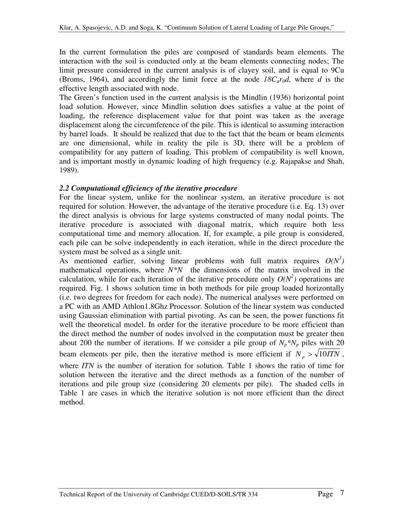
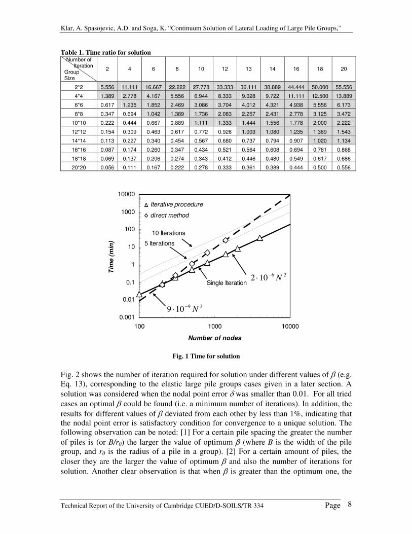
In the current formulation the piles are composed of standards beam elements. The interaction with the soil is conducted only at the beam elements connecting nodes; The limit pressure considered in the current analysis is of clayey soil, and is equal to 9Cu (Broms, 1964), and accordingly the limit force at the node 18Cur0d, where d is the effective length associated with node. The Green’s function used in the current analysis is the Mindlin (1936) horizontal point load solution. However, since Mindlin solution does satisfies a value at the point of loading, the reference displacement value for that point was taken as the average displacement along the circumference of the pile. This is identical to assuming interaction by barrel loads. It should be realized that due to the fact that the beam or beam elements are one dimensional, while in reality the pile is 3D, there will be a problem of compatibility for any pattern of loading. This problem of compatibility is well known, and is important mostly in dynamic loading of high frequency (e.g. Rajapakse and Shah, 1989). 2.2 Computational efficiency of the iterative procedure For the linear system, unlike for the nonlinear system, an iterative procedure is not required for solution. However, the advantage of the iterative procedure (i.e. Eq. 13) over the direct analysis is obvious for large systems constructed of many nodal points. The iterative procedure is associated with diagonal matrix, which require both less computational time and memory allocation. If, for example, a pile group is considered, each pile can be solve independently in each iteration, while in the direct procedure the system must be solved as a single unit. As mentioned earlier, solving linear problems with full matrix requires O(N3) mathematical operations, where N*N the dimensions of the matrix involved in the calculation, while for each iteration of the iterative procedure only O(N2) operations are required. Fig. 1 shows solution time in both methods for pile group loaded horizontally (i.e. two degrees for freedom for each node). The numerical analyses were performed on a PC with an AMD Athlon1.8Ghz Processor. Solution of the linear system was conducted using Gaussian elimination with partial pivoting. As can be seen, the power functions fit well the theoretical model. In order for the iterative procedure to be more efficient than the direct method the number of nodes involved in the computation must be greater then about 200 the number of iterations. If we consider a pile group of Np*Np piles with 20 beam elements per pile, then the iterative method is more efficient if ITNN p 10� , where ITN is the number of iteration for solution. Table 1 shows the ratio of time for solution between the iterative and the direct methods as a function of the number of iterations and pile group size (considering 20 elements per pile). The shaded cells in Table 1 are cases in which the iterative solution is not more efficient than the direct method.
Klar, A. Spasojevic, A.D. and Soga, K. “Continuum Solution of Lateral Loading of Large Pile Groups,”
Technical Report of the University of Cambridge CUED/D-SOILS/TR 334 Page 8
Table 1. Time ratio for solution Number of
Iteration Group Size
2 4 6 8 10 12 13 14 16 18 20
2*2 5.556 11.111 16.667 22.222 27.778 33.333 36.111 38.889 44.444 50.000 55.556
4*4 1.389 2.778 4.167 5.556 6.944 8.333 9.028 9.722 11.111 12.500 13.889
6*6 0.617 1.235 1.852 2.469 3.086 3.704 4.012 4.321 4.938 5.556 6.173
8*8 0.347 0.694 1.042 1.389 1.736 2.083 2.257 2.431 2.778 3.125 3.472
10*10 0.222 0.444 0.667 0.889 1.111 1.333 1.444 1.556 1.778 2.000 2.222
12*12 0.154 0.309 0.463 0.617 0.772 0.926 1.003 1.080 1.235 1.389 1.543
14*14 0.113 0.227 0.340 0.454 0.567 0.680 0.737 0.794 0.907 1.020 1.134
16*16 0.087 0.174 0.260 0.347 0.434 0.521 0.564 0.608 0.694 0.781 0.868
18*18 0.069 0.137 0.206 0.274 0.343 0.412 0.446 0.480 0.549 0.617 0.686
20*20 0.056 0.111 0.167 0.222 0.278 0.333 0.361 0.389 0.444 0.500 0.556
0.001
0.01
0.1
1
10
100
1000
10000
100 1000 10000
Number of nodes
Tim
e (m
in)
Iterative procedure
direct method
26102 N��
39109 N��
Single Iteration
5 Iterations
10 Iterations
Fig. 1 Time for solution
Fig. 2 shows the number of iteration required for solution under different values of � (e.g. Eq. 13), corresponding to the elastic large pile groups cases given in a later section. A solution was considered when the nodal point error � was smaller than 0.01. For all tried cases an optimal � could be found (i.e. a minimum number of iterations). In addition, the results for different values of � deviated from each other by less than 1%, indicating that the nodal point error is satisfactory condition for convergence to a unique solution. The following observation can be noted: [1] For a certain pile spacing the greater the number of piles is (or B/r0) the larger the value of optimum � (where B is the width of the pile group, and r0 is the radius of a pile in a group). [2] For a certain amount of piles, the closer they are the larger the value of optimum � and also the number of iterations for solution. Another clear observation is that when � is greater than the optimum one, the

Klar, A. Spasojevic, A.D. and Soga, K. “Continuum Solution of Lateral Loading of Large Pile Groups,”
Technical Report of the University of Cambridge CUED/D-SOILS/TR 334 Page 9
number of iterations for solution increases more or less linearly with �. One should remember that all of the above values were obtained for maximum nodal error �=0.01. A less rigorous demand will decrease significant the number of iterations. Increasing the tolerance to �=0.05 can decrease the number of iterations by more than half, consequently leading to less than half the calculation time, making the iterative scheme even more appealing. For example, the case of B/r0=150, S/r0=7.5 (20*20 pile group) ,where S is the spacing between the piles, was solved with �=25 and reached �=0.05 in 20 iteration, for which the deviation in pile group stiffness from the �=0.01 solution was only 0.85%. A �=0.18 was obtained after 10 iterations and the stiffness deviation from the �=0.01 solution was only 5%. Considering Table 1 for time saving, it seems reasonable in some cases to substitute accuracy for computational efficiency.
0
5
10
15
20
25
0 1 2 3 4 5 6 7 8 9 10 11 12ββββ
Num
ber
of it
erat
ions
Single pileS/r0=30, B/r0=60, 2*2S/r0=15, B/r0=30, 2*2S/r0=7.5, B/r0=15, 2*2S/r0=30, B/r0=120, 4*4S/r0=15, B/r0=60, 4*4S/r0=7.5, B/r0=30, 4*4S/r0=30, B/r0=300, 10*10S/r0=15, B/r0=150, 10*10S/r0=7.5, B/r0=75, 10*10
Fig. 2 Influence of ���� on iteration procedure, ����=0.01.
3. Validation To validate the operation of the written code, several problems were considered, both for single pile and pile groups. 3.1 Single pile – Elastic response Fig. 3 shows flexibility coefficient from different analysis methods of elastic material. The coefficients involved in the pile head defalcation are as follows:
30
2220
21
20
120
11
rEM
arE
Pa
rEM
arE
PaU
ss
ss
���
��
Eq. 18
where U is � are the horizontal translation and rotation of the pile’s head, P and M are the horizontal force and moment acting on the head of the pile, r0 is the pile radius and Es is the Young’s modulus of the soil. The analyses results, shown in Fig. 2, are for pile with slenderness ratio of L/r0=60 and is composed of 30 beam elements. The iterative procedure is compared with 3 different results: Poulos elastic solution, Kuhlemeyer

Klar, A. Spasojevic, A.D. and Soga, K. “Continuum Solution of Lateral Loading of Large Pile Groups,”
Technical Report of the University of Cambridge CUED/D-SOILS/TR 334 Page 10
(1979) rigorous finite element analysis, and Klar and Frydman (2002) relaxed finite different analysis, in which the continuum motion in the vertical direction is prevented. As can be seen the agreement is excellent. It should be noted that some of Poulos's results are considered to be in error due to numerical discretization effects (e.g. Kuhlemeyer, 1979).
0.001
0.01
0.1
1
100 1000 10000Ep/Es
a11,
a12,
a21,
a22
PoulosKuhlemeyerF.D., Klar and FrydmanIterative procedure
�s=0.5�s=0.4
�s=0.4�s=0.5
a11
a22
a12=a21
Fig. 3 Elastic solution
3.2 Single pile – Plastic response To extend the solution to the plastic case let us use both the secant stiffness method and the plasticity solution. It should be realized that generally these two systems are not identical. Only if {df} in Eqs.15 or 17 holds a consistent sign throughout the incremental loading the secant method (i.e. Eq. 14) and the plastic solution (i.e. Eqs. 15 or 17) will be identical, even when the plastic solution is obtained using single increment of loading. It will be shown later that this is not always the case for the soil-pile interaction problem. To normalize the plastic solutions let us consider a limit yield load derived from limit equilibrium conditions. The pile in the current calculation is elastic, hence it can not fail under bending moment, and as a result the limit load will correspond to the soil limit reaction. Fig. 4 shows the mechanism of failure assumed for the limit load of a free head pile, Py. This mechanism is similar to Broms (1964) mechanism of short pile, excluding the omission of the soil reaction near the surface. Note, Broms definition of short piles and long piles is different than that related to deformation analysis. Broms defines short piles as piles that do not fail under bending moment, while long piles in deformation analysis are piles that their length does not affect their response.
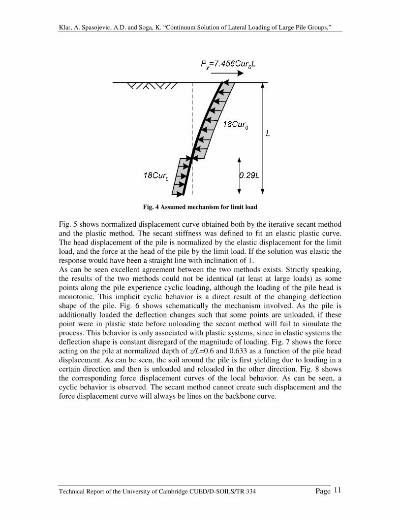
Klar, A. Spasojevic, A.D. and Soga, K. “Continuum Solution of Lateral Loading of Large Pile Groups,”
Technical Report of the University of Cambridge CUED/D-SOILS/TR 334 Page 11
Fig. 4 Assumed mechanism for limit load
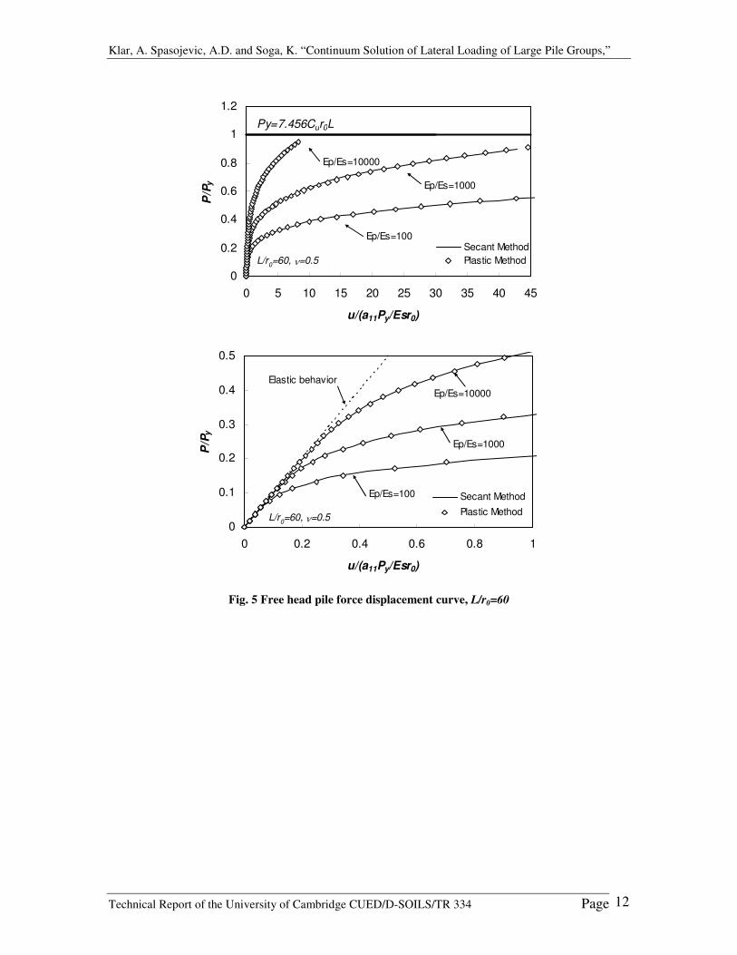
Fig. 5 shows normalized displacement curve obtained both by the iterative secant method and the plastic method. The secant stiffness was defined to fit an elastic plastic curve. The head displacement of the pile is normalized by the elastic displacement for the limit load, and the force at the head of the pile by the limit load. If the solution was elastic the response would have been a straight line with inclination of 1. As can be seen excellent agreement between the two methods exists. Strictly speaking, the results of the two methods could not be identical (at least at large loads) as some points along the pile experience cyclic loading, although the loading of the pile head is monotonic. This implicit cyclic behavior is a direct result of the changing deflection shape of the pile. Fig. 6 shows schematically the mechanism involved. As the pile is additionally loaded the deflection changes such that some points are unloaded, if these point were in plastic state before unloading the secant method will fail to simulate the process. This behavior is only associated with plastic systems, since in elastic systems the deflection shape is constant disregard of the magnitude of loading. Fig. 7 shows the force acting on the pile at normalized depth of z/L=0.6 and 0.633 as a function of the pile head displacement. As can be seen, the soil around the pile is first yielding due to loading in a certain direction and then is unloaded and reloaded in the other direction. Fig. 8 shows the corresponding force displacement curves of the local behavior. As can be seen, a cyclic behavior is observed. The secant method cannot create such displacement and the force displacement curve will always be lines on the backbone curve.
Klar, A. Spasojevic, A.D. and Soga, K. “Continuum Solution of Lateral Loading of Large Pile Groups,”
Technical Report of the University of Cambridge CUED/D-SOILS/TR 334 Page 12
0
0.2
0.4
0.6
0.8
1
1.2
0 5 10 15 20 25 30 35 40 45
u/(a11Py/Esr0)
P/P
y
Secant MethodPlastic Method
Py=7.456Cur0L
L/r0=60, �=0.5
Ep/Es=10000
Ep/Es=1000
Ep/Es=100
0
0.1
0.2
0.3
0.4
0.5
0 0.2 0.4 0.6 0.8 1
u/(a11Py/Esr0)
P/P
y
Secant MethodPlastic MethodL/r0=60, �=0.5
Ep/Es=10000
Ep/Es=1000
Ep/Es=100
Elastic behavior
Fig. 5 Free head pile force displacement curve, L/r0=60

Klar, A. Spasojevic, A.D. and Soga, K. “Continuum Solution of Lateral Loading of Large Pile Groups,”
Technical Report of the University of Cambridge CUED/D-SOILS/TR 334 Page 13
Fig. 6 Unloading of point A
-1.5
-1
-0.5
0
0.5
1
1.5
0 10 20 30 40 50
u/(a11Py/Esr0)
f/fy
z/l=0.6
z/l=0.633
Ep/Es=1000; L/r0=60
Fig. 7 Loading along the pile as function of head displacement
Klar, A. Spasojevic, A.D. and Soga, K. “Continuum Solution of Lateral Loading of Large Pile Groups,”
Technical Report of the University of Cambridge CUED/D-SOILS/TR 334 Page 14
-1.5
-1.0
-0.5
0.0
0.5
1.0
1.5
-4.0 -2.0 0.0 2.0 4.0 6.0
(u-u A )/f yG i,i
f/fy
z/l=0.6
z/l=0.633Ep/Es=1000; L/r0=60
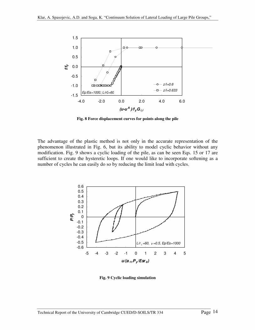
Fig. 8 Force displacement curves for points along the pile
The advantage of the plastic method is not only in the accurate representation of the phenomenon illustrated in Fig. 6, but its ability to model cyclic behavior without any modification. Fig. 9 shows a cyclic loading of the pile, as can be seen Eqs. 15 or 17 are sufficient to create the hysteretic loops. If one would like to incorporate softening as a number of cycles he can easily do so by reducing the limit load with cycles.
-0.6-0.5-0.4-0.3-0.2-0.1
00.10.20.30.40.50.6
-5 -4 -3 -2 -1 0 1 2 3 4 5
u/(a 11Py/Esr 0)
P/P
y
L/r 0=60, ν =0.5, Ep/Es=1000
Fig. 9 Cyclic loading simulation
Klar, A. Spasojevic, A.D. and Soga, K. “Continuum Solution of Lateral Loading of Large Pile Groups,”
Technical Report of the University of Cambridge CUED/D-SOILS/TR 334 Page 15
3.3 Comparison with common practice methods API current practice employs the use of nonlinear Winkler model. For static loading in soft clays Matlock’s (1970) p-y curve is suggested:
yo
pr
yp
3/1
5055.0 ��
�
����
��
� Eq. 19
Where p is the pressure per unit length acting on the pile and y is the pile displacement, �50 is the strain corresponds to one-half of the maximum principal stress difference, and py is the limit pressure, calculated as the minimum between wedge type failure mechanism and a flow around mechanism }5.0'26,18{ 000 zCuzrCurCurMinp y ��� . Since in the current analysis only the “flow around” mechanism is considered we shall limit Matlock’s p-y curve to that mode of failure. Note, the presented method can account for any prescribed limit load; hence the two different mechanism can still be included. However, in this case the logical reasoning (i.e. local plastic failure) does not apply and the model is less rigorous. For sake of comparison between the methods let us assume that the soil is elasto-plastic, correspondingly �50 is equal to Cu/Es. Fig. 10 shows comparison of API model with the continuum solution. As can be seen, once the continuum solution ceases to be completely elastic (i.e. breaks from the straight line) the agreement is excellent. However, for point before that state the API model results in a stiffer system. It is not suggested that in reality this is not the case. However, theoretically, Matlock’s p-y curve must over predict the stiffness at small displacement as
!"## yp / when 0"y . If, however, the API model represents the true soil-pile behavior, then the current analysis indicates that a choice of Es, for the continuum solution, according to �50 will result in a more flexible system for small loads and a well one for large loads.

Klar, A. Spasojevic, A.D. and Soga, K. “Continuum Solution of Lateral Loading of Large Pile Groups,”
Technical Report of the University of Cambridge CUED/D-SOILS/TR 334 Page 16
0
0.2
0.4
0.6
0.8
1
1.2
0 10 20 30 40
u/(a 11Py/Esr 0)
P/P
y
API (Winkler Model)Contiuum solution
Py=7.456C ur 0L
Ep/Es=10000
Ep/Es=1000
Ep/Es=100
L/r 0=60, ν =0.5
0
0.1
0.2
0.3
0.4
0.5
0.6
0 0.2 0.4 0.6 0.8 1
u/(a 11Py/Esr 0)
P/P
y
API (Winkler Model)Contiuum solution
Ep/Es=10000 Ep/Es=1000
Ep/Es=100
L/r 0=60, ν =0.5
Fig. 10 Comparison with API method
Klar, A. Spasojevic, A.D. and Soga, K. “Continuum Solution of Lateral Loading of Large Pile Groups,”
Technical Report of the University of Cambridge CUED/D-SOILS/TR 334 Page 17
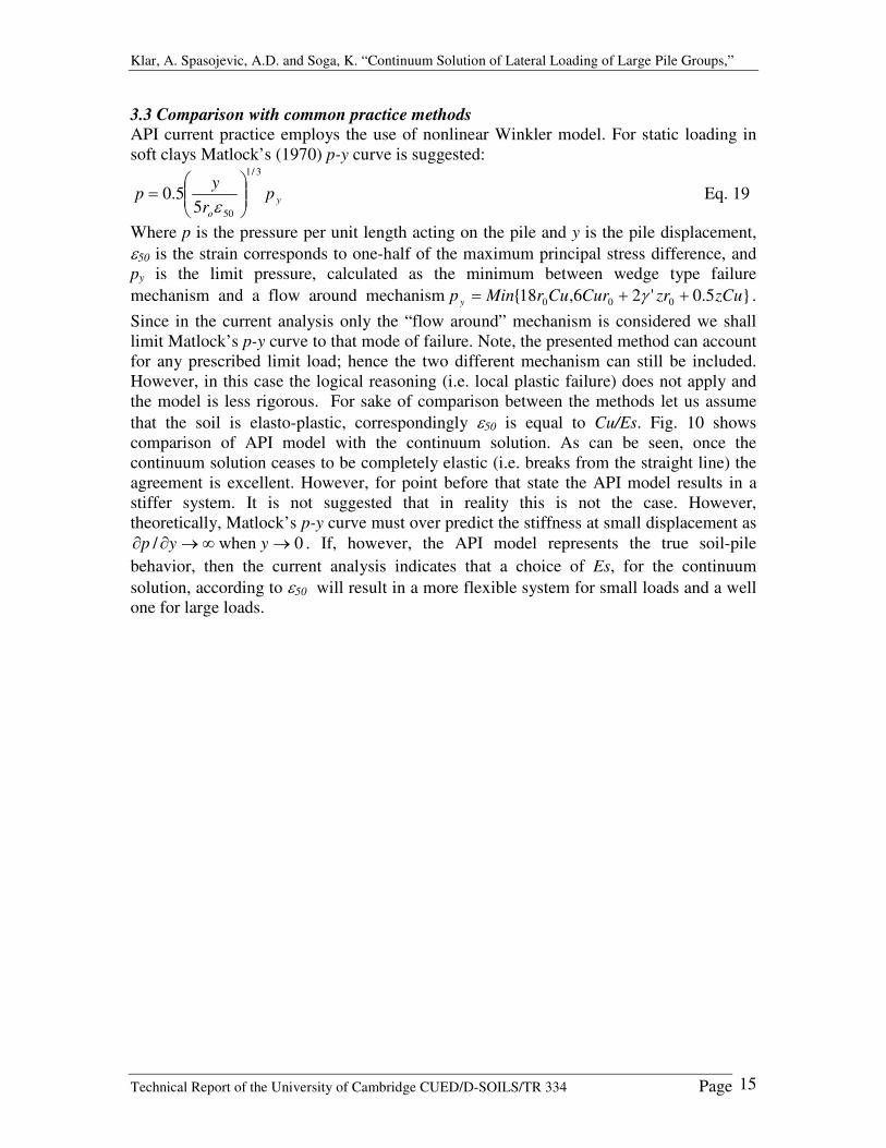
3.4 Pile-soil-pile interaction Before referring to the large pile group solution, let us consider the most simple case of pile group – two piles. In addition of allowing validation of the correctness of the code for modeling pile-soil-pile interaction, this case is important since it relates to the super position method, in which the interaction between every two piles in a group is superimpose for the group response. In the superposition method interaction factor are used to obtain the behavior of the group, }]{[}{ Pu $�� (where � is the flexibility of a single pile). The interaction factor $i,j is defined as the additional displacement to pile i due to unit loading on pile j, $i,i is always equal to 1. Since it is so popular, it will be used for comparison also in the following section dealing with large pile groups. Fig. 11 shows comparison between the Randolph’s (1981) interaction factors, Poulos (1971), and values obtained using the current method. As can be seen the current method results with interaction factor similar to those of Poulos (1971). Randolph’s interaction factors agree well for large pile spacing but slightly over predict interaction of closely spaced piles.
00.10.20.30.40.50.60.70.80.9
1
0 10 20 30 40
S/r 0
Inte
ract
rion
fact
or
Ep/Es=8000, L/r0=50Ep/Es=200 , L/r0=20Ep/Es=8000, L/r0=50 - PoulosEp/Es=200 , L/r0=20 - PoulosEp/Es=8000, L/r0=50 - Randolph Ep/Es=200 , L/r0=20 - Randolph
Fig. 11 Comparison of interaction factors for fixed head piles, ����=0.5 (piles are lined with the direction
of loading). 4. Large pile Groups 4.1 Elastic behavior In the present section we shall view the response of a large pile group based on superposition method and the method presented in the previous sections. Let us consider a case of symmetric pile group, N*N, with a rigid cap of size B*B. A load per unit area, or average horizontal stress, may be defined as PA=PG/B2. PG is the force acting on the cap and is equal also to N times the average load on a pile, �� aviG NPPP , where N is the number of piles. Assuming the symmetric configuration shown in Fig. 12 N=(B/S)2
, where S is the spacing between the piles, and as a result 2/ SPP avA � . If the pile group cap is rigid, the head displacements of all piles are equal to the cap displacement UG which is:
AGG PBPU 2%�%� Eq. 20

Klar, A. Spasojevic, A.D. and Soga, K. “Continuum Solution of Lateral Loading of Large Pile Groups,”
Technical Report of the University of Cambridge CUED/D-SOILS/TR 334 Page 18
where % is the pile group flexibility. If no interaction occurs between the piles �� �� // GGG NUUP , where � is single fixed head pile flexibility. An efficiency factor may be considered:
%����
��
��&
NNUP
UU
PwithP
G
G
constPG
G
ConstUG
G
GG
1)ninteractiowith (
)ninteractiowithout ()ninteractiowithout (
)ninteractio ( Eq. 21
Note that the solution without interaction is still affected by the spacing between the piles as it defines the number of piles supporting the cap. Relations between % and & can be developed as a function of the ratios B/r0 and S/r0:
20
20
2 )/()/(111
rBrS
SBN &
&&�
�
��
���
���
% Eq. 22
Note that for static loading & is bounded by 1�& , as a result %/� has a lower bound. It will be shown later that %/� becomes insensitive to the spacing between the piles as the pile group becomes larger. The argument for that might be explained from the above equation; as the pile are spaced closer the efficiency of each pile is reduced, however the total response is balanced by the increased number of pile such that N& is more or less constant.
Fig. 12 Notation and geometry of symmetric pile group
One of the common techniques for solution of pile groups is the superposition method (e.g. Poulos, 1971; Randolph, 1981). One should realize that this method is not rigorous since it does not consider superposition of loads on a single system, but instead superimpose pile responses; i.e. whenever two piles are interacting they are not “aware” of the existence other piles.

Klar, A. Spasojevic, A.D. and Soga, K. “Continuum Solution of Lateral Loading of Large Pile Groups,”
Technical Report of the University of Cambridge CUED/D-SOILS/TR 334 Page 19
For rigid cap pile group the stiffness is �
�N
i
N
jjiGG PU
1,/ �� , where �i,j are the
component of the inverse interaction factors matrix $'(As a result: 1
1,
�
����
����
��
%
N
i
N
jji�
� Eq. 23
Let us adopt Randolph’s (1981) popular superposition factor for fixed pile head:
) *Rr
EsEp
f02
7/1
cos175.01
126.0 +
��
$ ���
���
��
�� Eq. 24
Where + is the angle between the line joining the pile centers and the direction of loading, and pile and R is the distance between the piles. Since the superposition method is still popular and more computationally efficient, it will be used to for comparison. Fig. 13 shows normalized pile group flexibility %/� for B/r0=20,40,60,80,100,150 and for pile spacing S/r0 up to 30 both for the superposition method (e.g. SP) and the rigorous one. Few trends can be immediately recognized: [1] For a certain pile spacing, the larger the pile group is the stiffer it is, [2] For a certain pile group dimension, B/r0, the smaller the spacing between the piles is the stiffer it is. However, [3] the larger the pile group dimension, B/r0, is the change of stiffness with spacing is less noticeable.
0
0.1
0.2
0.3
0.4
0.5
0.6
2 4 6 8 10 12 14 16 18 20 22 24 26 28 30S/r0
Λ/λ
Λ/λ
Λ/λ
Λ/λ
B/r0=20 - SP B/r0=20 - RigorousB/r0=40 -SP B/r0=40 - RigorousB/r0=60 - SP B/r0=60 - RigorousB/r0=80 - SP B/r0=80 - RigorousB/r0=100 - SP B/r0=100 - RigorousB/r0=150 - SP B/r0=150 - Rigorous
Fig. 13 Normalized pile group flexibility, Ep/Es=1000 L/r0=60
The third trend suggests that if B/r0 approaches infinite the pile spacing should not have effect at all. If B/r0 approaches infinite the pile group is also infinite and for that case each pile in the group behaves identically to all other piles. For that case flexibility of the system can be evaluated by a simpler expression than that shown in Eq. 23:

Klar, A. Spasojevic, A.D. and Soga, K. “Continuum Solution of Lateral Loading of Large Pile Groups,”
Technical Report of the University of Cambridge CUED/D-SOILS/TR 334 Page 20
��%
$$
� 20
20
)/()/(
rBrS
N Eq. 25
Where, $ is the interaction factor of all other piles with a certain pile. Considering pile numbering as in Fig. 13, and Randolph’s interaction factors, Eq. 25 is equal to
7/1
0
2222
20
20
20
75.011
26.0
11
1)/()/(
��
���
��
��
,,,
-
.
///
0
1
��
���
����
�
����
% !
�!�
!
�
�!�
EsEp
A
lklkk
ASr
rBrS
N kkl
l
��
$
� Eq. 26
The series in the above equation does not converge, hence %/�(has no limit for infinite pile group. However, for the value of (B/r0)(%/�), there is a limit when !")/( 0rB :
AZr
S
lklkk
ZA
rB Z
Zk
Z
klZlZ
rB
287.511
11
limlim0
2/
2/
2/
02/ 2222
2
00
���
���
����
�
���
% ��
�
��!"!" � Eq. 27
As can be seen the limit value of (B/r0)(%/�) is not a function of piles spacing. No correction for closely spaced piles was considered; however, since the solution is not dependent on spacing, it still holds for interaction factors values for which no correction was required. One should realize that this result is based on the superposition assumption and Randolph’s interaction factor, and is not necessarily the true behavior of infinite pile group. There is additional limit that can be analytically calculated. If the pile group is extremely large and is placed in a semi infinite continuum, then the result should also correspond to horizontal loading of a rigid rectangular on the surface since the ratio l/B approaches zero. Barkan (1962) gave approximation for the horizontal loading of rigid rectangle on the surface:
QEsBLx
h�
23
21�� Eq. 28
Where 3h is the displacement and Q is the horizontal load, B and L are the dimension of the rectangle, �x is a factor depending on the both B/L and � and for B/L=1 and �=0.5 its value is 0.704. By manipulating the above relation one can achieve the following limit for the pile group.
EsrrB
xrB
0
2
0
1lim0
��2
��
�%
!"
Eq. 29
Randolph (1981) expression for the stiffness of a fixed head single pile is:
��
��
� 2275.01
75.011
229.61
0
7/1
��
��
���
��
��� sEr
EsEp
k Eq. 30
Introducing it to Eq. 29 results in:
AArB
x
12.575.025.01
24.55.02
0
�
���
�% �
���
� Eq. 31

Klar, A. Spasojevic, A.D. and Soga, K. “Continuum Solution of Lateral Loading of Large Pile Groups,”
Technical Report of the University of Cambridge CUED/D-SOILS/TR 334 Page 21
Remarkably we achieve a close value to that obtained from the infinite series of interaction factors. Disregarding the values, these limits suggests that the ratio (B/r0)(%/�) should reach a limit when as the pile group behave more and more as a large group. Fig. 15 shows the values of Fig. 13 multiplied by B/r0.
Fig. 14 Numbering of piles
4
6
8
10
12
14
16
18
20
2 4 6 8 10 12 14 16 18 20 22 24 26 28 30S/r0
)) ))B/r
0 *)*) *)*)%% %%44 44 �� ��
** **
B/r0=20 - SP B/r0=20 - RigorousB/r0=40 -SP B/r0=40 - RigorousB/r0=60 - SP B/r0=60 - RigorousB/r0=80 - SP S/r0=80 - RigorousB/r0=100 - SP B/r0=100 - RigorousB/r0=150 - SP B/r0=150 - Rigorous
Fig. 15 Normalized pile group flexibility, Ep/Es=1000 L/r0=60
As can be clearly seen from Fig. 15 as the size of the pile group increase the flexibility or stiffness is less sensitive to the pile spacing. It seems that this insensitivity is more pronounce in the superposition method using Randolph’s interaction factors for small pile spacing. Nevertheless, as the pile group becomes larger the rigorous method also shows this pattern of behavior. It should be noted that the values obtained for the superposition method are still smaller than the limit value from the above equations. This is probably because a correction method is involved and that the pile group is not large enough to
Klar, A. Spasojevic, A.D. and Soga, K. “Continuum Solution of Lateral Loading of Large Pile Groups,”
Technical Report of the University of Cambridge CUED/D-SOILS/TR 334 Page 22
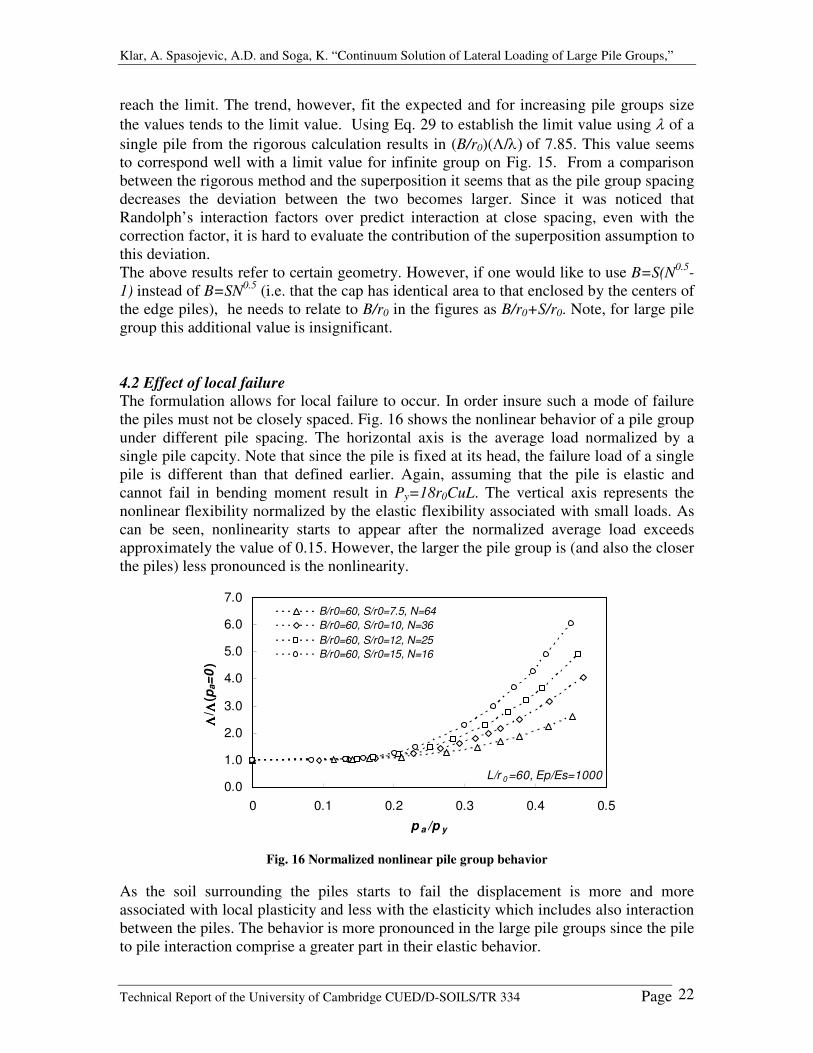
reach the limit. The trend, however, fit the expected and for increasing pile groups size the values tends to the limit value. Using Eq. 29 to establish the limit value using � of a single pile from the rigorous calculation results in (B/r0)(%/�*(of 7.85. This value seems to correspond well with a limit value for infinite group on Fig. 15. From a comparison between the rigorous method and the superposition it seems that as the pile group spacing decreases the deviation between the two becomes larger. Since it was noticed that Randolph’s interaction factors over predict interaction at close spacing, even with the correction factor, it is hard to evaluate the contribution of the superposition assumption to this deviation. The above results refer to certain geometry. However, if one would like to use B=S(N0.5-1) instead of B=SN0.5 (i.e. that the cap has identical area to that enclosed by the centers of the edge piles), he needs to relate to B/r0 in the figures as B/r0+S/r0. Note, for large pile group this additional value is insignificant. 4.2 Effect of local failure The formulation allows for local failure to occur. In order insure such a mode of failure the piles must not be closely spaced. Fig. 16 shows the nonlinear behavior of a pile group under different pile spacing. The horizontal axis is the average load normalized by a single pile capcity. Note that since the pile is fixed at its head, the failure load of a single pile is different than that defined earlier. Again, assuming that the pile is elastic and cannot fail in bending moment result in Py=18r0CuL. The vertical axis represents the nonlinear flexibility normalized by the elastic flexibility associated with small loads. As can be seen, nonlinearity starts to appear after the normalized average load exceeds approximately the value of 0.15. However, the larger the pile group is (and also the closer the piles) less pronounced is the nonlinearity.
0.0
1.0
2.0
3.0
4.0
5.0
6.0
7.0
0 0.1 0.2 0.3 0.4 0.5
p a /p y
ΛΛ ΛΛ/ ΛΛ ΛΛ
(pa=
0)
B/r0=60, S/r0=7.5, N=64B/r0=60, S/r0=10, N=36B/r0=60, S/r0=12, N=25B/r0=60, S/r0=15, N=16
L/r 0 =60, Ep/Es=1000
Fig. 16 Normalized nonlinear pile group behavior
As the soil surrounding the piles starts to fail the displacement is more and more associated with local plasticity and less with the elasticity which includes also interaction between the piles. The behavior is more pronounced in the large pile groups since the pile to pile interaction comprise a greater part in their elastic behavior.

Klar, A. Spasojevic, A.D. and Soga, K. “Continuum Solution of Lateral Loading of Large Pile Groups,”
Technical Report of the University of Cambridge CUED/D-SOILS/TR 334 Page 23
Fig. 17 shows the ratio %/�, where in this case � is the nonlinear flexibility of a single pile under the average load (i.e. PG/N). As can be seen from Eq. 25, %/� can be defined as the average interaction factor. As the normalized average load increases the interaction is reduced, and the pile group behavior becomes more and more sensitive to the pile spacing. For example, the pile group with S/r0=12 is only about 20% more flexible than that of S/r0=7.5 for small loading, while for large loading it is more than 2.5 times greater. In practice, although not rigorous, interaction factor and the superposition method are used sometimes to obtain the nonlinear behavior of the pile groups. It is clear that in that case, an overestimation of pile group flexibility results.
0.00
0.02
0.04
0.06
0.08
0.10
0.12
0.14
0.16
0 0.1 0.2 0.3 0.4 0.5
p a /p y
ΛΛ ΛΛ/ λλ λλ
(pa)
B/r0=60, S/r0=7.5, N=64B/r0=60, S/r0=10, N=36B/r0=60, S/r0=12, N=25B/ro=60, S/r0=15, N=16
Lines of no interaction (i.e. λp a =Λp a N )
S/r 0 =12S/r 0 =10S/r 0 =7.5
S/r 0 =15
L/r 0 =60, Ep/Es=1000
Fig. 17 Normalized interaction behavior, L/r0=60, Ep/Es=1000
5. Summary and conclusions Large pile groups under static horizontal loading were solved. The solution employed an iterative procedure which reduce both computation time and memory allocation. Investigation of pile spacing and pile group size was conducted and the following trends were found: [1] For a certain pile spacing, the larger the pile group is, the stiffer it is, [2] For a certain pile group dimension, B/r0, the smaller the spacing between the piles, the stiffer it is. However, [3] the larger the pile group dimension, B/r0, is, the change of stiffness with spacing is less noticeable. The last trend was supported by referring to infinite pile group and solving it using the superposition method which resulted with the spacing term diminished. The investigation extended to include local failure around the pile. Obviously, this sort of failure corresponds more to distant piles rather than closely spaced piles. It was found that the greater the number of piles in a group, the less it is sensitive to failure; as the soil surrounding the piles starts to fail the displacement is more and more associated with local plasticity and less with the elasticity which includes significant interaction between the piles. In addition to the above observations, it was found in the process of validating the code that under elasto-plastic state, the soil along the pile may experience cyclic loading although the pile itself is monotonically loaded.

Klar, A. Spasojevic, A.D. and Soga, K. “Continuum Solution of Lateral Loading of Large Pile Groups,”
Technical Report of the University of Cambridge CUED/D-SOILS/TR 334 Page 24
6. References Barkan, D.D. (1962) “Dynamics of bases and foundations,” McGraw Hill, New York. Broms, B.B. (1964) “Lateral Resistance of Piles in Cohesive Soils,” Journal of the Soil Mechanics and Foundations Division, ASCE, Vol. 90(2) pp.27-63 Chow Y.K. (1987) “Iterative Analysis of Pile-Soil-Pile Interaction,” Geotechnique 37(3) pp.321-333 Klar, A. and Frydman, S. (2002) “Three-Dimensional Analysis of Lateral Pile Response using Two-Dimensional Explicitly Numerical Scheme,” J. Geotechnical and Geo environment Engineering, ASCE Vol. 128(GT9) pp. 775-784 Klar, A., Frydman, S. and Baker, R. (2004) “Seismic Analysis of Infinite Pile Group in Liquefiable Soil,” Soil Dynamics and Earthquake Engineering. In press. Kuhlemeyer, R. (1979) ‘‘Static and dynamic laterally loaded floating piles.’’ J. Geotech. Eng., 105(2), 289–304. Matlock, H. (1970) “Correlations for Design of Laterally Loaded Piles in Soft Clay,” Paper No. OTC 1204, Proceeding, Second Annual Offshore Technology Conference, Houston, Texas, Vol. 1 pp. 577-594 Mindlin R.D., (1936) “Force at a Point in the Interior of a Semi-Infinite Solid,” Journal of Applied Physics, Vol. 7, No. 5 pp-195-202 Poulos, H.G. (1971) “Behavior of Laterally Loaded Piles: I – Single Piles,” Journal of the Soil Mechanics and Foundation Division, Vol. 97. No. 5 pp.711-731 Rajapakse, R. K. N. D., and Shah, A. H. (1989) ‘‘Impedance curves for an elastic pile.’’ Soil Dyn. Earthquake Eng., 8(3), 145–152. Randolph, M.F. (1981) “The Response of Flexible Piles to Lateral Loading,” Geotechnique Vol. 31(2) pp. 247-259


