Contract Mo. EM3C­0008­D (Β)

NUMERICAL 3­D SEISMIC MODELLIMG

A. BEHLE1, J. CARCIOHE3, H. FRETER1, Ζ. KOREH3 D. KOSLOFF2, Β. KUMMER1 and E. TESSMER1

1 Hamburg University 3 Tel Aviv University and Hamburg University

Summary The objective of this research project is to develop and test algo­rithms and computer programs that enable a realistic modelling of seismic wave propagation in 3­D (three­dimensional) laterally inho­mogeneous media. Various material rheologies are considered: acou­

stic/elastic, viscoacoustic/­elastic, anisotropic. The numerical so­lution of the equations of motion is obtained by the Fourier method. Hew time integration schemes are developed which are superior to the conventional finite difference time stepping approach. Time sections and snapshots of the wavefield for 2­D and 3­D laterally inhomogeneous media of different rheologies are presented.

1. IMTRODUCTIOM The growing importance of 3­D seismic surveys in hydrocarbon explora­tion requires the development of appropriate forward modelling techni­ques for quality control and interpretation of results. Appropriate in our opinion is a wide­band technique suitable for the simulation of the full wave response in 3­D generally varying media and allowing the implementation of various rheologies. Numerical methods which are based on finite difference techniques can­not be applied to 3­D exploration models of realistic size and rheo­logy because they require a computing capacity which cannot be met even by the supercomputers available today. The proposed approach is based on the Fourier method [1]. The main advantage of this method over finite difference techniques is that the ratio of minimum wave length to the spatial increment is three times smaller. This permits a significant reduction of the working space dimensions so that a seismic modelling of realistic 3­D structures can

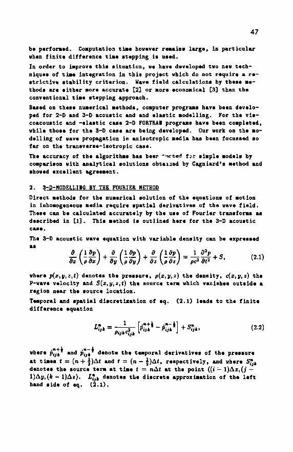
47 be performed. Computation time however remain· large, in particular when finite difference time stepping is used. In order to improve thia situation, we have developed two new tech­nique· of ti«· integration in thi· project which do not require a re­strictiv* stability criterion. Wave field calculation· by these me­thod· are either more accurate [2] or more economical [3] than the conventional time stepping approach. Based on these numerical methods, computer programs have been develo­ped for 2­D and 3­D acoustic and and elastic modelling. For the vis­coacoustic and ­elastic case 2­D FORTRAN programs have been completed, while those for the 3­D case are being developed. Our work on the mo­delling of wave propagation in anisotropic media has been focussed so far on the tranaverse­isotropic case. The accuracy of the algorithms has been "­wrteri for simple models by comparison with analytical solutions obtained by Cagniard's method and showed excellent agreement.

2. 3­D­MODELLING BY THE FOURIER METHOD Direct methods for the numerical solution of the equations of motion in inhomogeneous media require spatial derivatives of the wave field. These can be calculated accurately by the use of Fourier transforms as described in [1]. This method is outlined here for the 3­D acoustic case. The 3­D acoustic wave equation with variable density can be expressed

Õx \pÕx) + dy \pdy) + dz \pdz) " po' dt' + '

{ '

where p(x,y,z,t) denotes the pressure, p(x,y,z) the density, c(x,y,z) the P­wave velocity and S(x,y,z,t) the source term which vanishes outside a region near the source location. Temporal and spatial discretization of eq. (2.1) leads to the finite difference equation

L" = rh­ ft* ­ &]

+ s*» ( 2

·2 )

where |>yj and Py» denote the temporal derivatives of the pressure at time· t = (η + *)Δί and f = (η ­ j)A<, respectively, and where S*à denotes the source term at time t = ηΔί at the point ((i ­ l)Ax,(j ­

1)Δν,(fc ­ 1)Δ*). ¿'t denotes the discrete approximation of the left hand side of eq. (2.1).

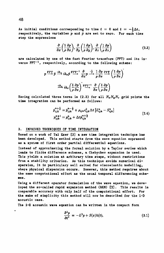
48 As initial conditions corresponding to time t = 0 and t = —^At, respectively, the variables ρ and ρ are set to zero. For each time step the expressions

dx\pdx)'dy Xpoy)' dz\pdz) ^

are calculated by use of the fast Fourier transform (FFT) and its in­verse FFT­1

, respectively, according to the following scheme:

FFT . iks ., . FFT­ 1 d 'ρ 1 Op FFT

ρ — ► ρ — ► ikxp — ► —ρ — > - - ► οχ ρ αχ

\pdxj

•ikş ., fl£p\ FFT"1 d ί\ dp\ x\pdxJ dx\pdx)

Having calculated three terms in (2.3) for all NxNyNz grid points the time integration can be performed as follows:

PÏk* = P*hlέ + PüK$kto [Vjk - S?jk]

Pijk ­ Pi]k + At

Pijk

3. IMPROVED TECHNIQUES OF TIME INTEGRATION Based on a work of Tal Ezer [3] a new time integration technique has been developed. This method starts from the wave equation expressed as a system of first order partial differential equations. Instead of approximating the formal solution by a Taylor series which leads to finite difference schemes, a Chebychev expansion is used. This yields a solution at arbitrary time steps, without restrictions from a stability criterion. As this technique avoids numerical di­spersion, it is particulary well suited for viscoelastic modelling, where physical dispersion occurs. However, this method requires about the same computational effort as the usual temporal differencing sche­mes. Using a different operator formulation of the wave equation, we deve­loped the so­called rapid expansion method (REM) [2]. This results in comparable accuracy with only half of the computational effort. For the sake of simplicity this method will now be described for the 1­D acoustic case. The 1­D acoustic wave equation can be written in the compact form

j * = -l2p+S(x)h(t), (3.1)

49

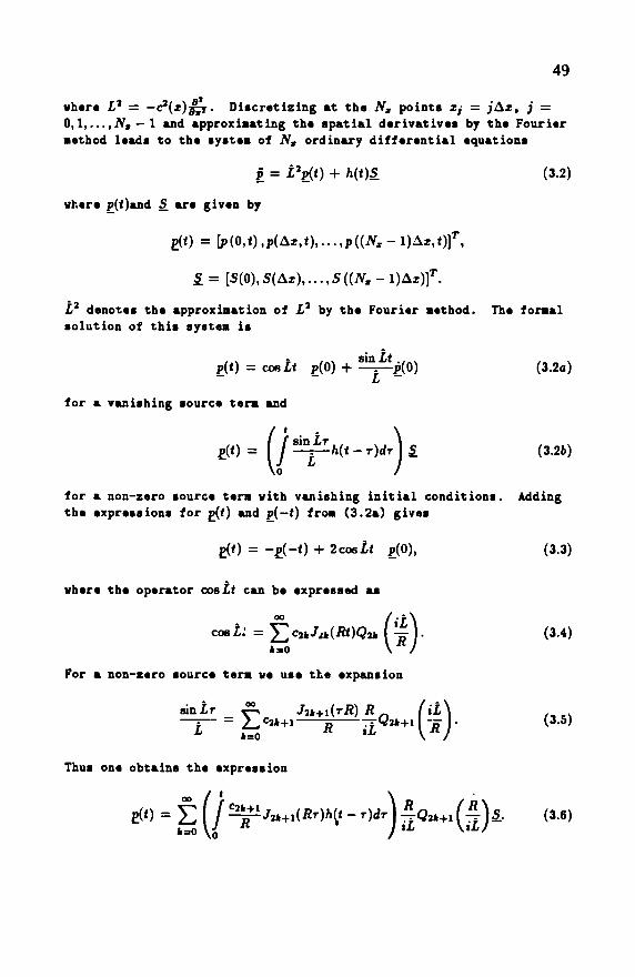
where L1 — ­ < ^ ( Γ ) ^ Τ · Discretizing at the NM pointa x¡ = jAx, j =

0,1 , . . . , jy, — 1 and approximating the spatial derivatives by the Fourier ■ethod leads to the system of Ns ordinary differential aquations

£ = VM + h{t)S (3.2)

where p(t)and Ş are given by

£(<) = \p(0,t),p(Ax,t),...,p((Nx­l)^x,t)]T,

S = [S(0), S{Ax) S ((ΛΓ, ­ 1)Δζ)]τ.

¿3 denotes the approximation of X

2 by the Fourier method. The formal solution of this system i s

¿t) = ccett £(0) + ^ ¿ ( 0 ) (3.2a) L·

for a varnishing source term and

£(<) = ( ƒ ^y^M* - r)dr J S. (3.26)

for a non-zero source term with vanishing in i t ia l conditions. Adding the expressions for p(t) and p(—t) from (3.2a) gives

£(') = - £ ( - 0 + 2coe£< p(0), (3.3)

where the operator cos It can be expressed as

cosi: = ¿ e » J r t ( Ä ) Q a . Í ^ J . (3.4)

For a non-zero source term we use the expansion

sin LT _ ^ _ Jn+ijrR) R n ('il\

— - ¿ C a * + 1 — R — a Q u + l [ R ] · (35)

Thus one obtains the expression

EO = Σ ( ƒ ^Ju+iWK} - T)dr\ 4 Q « + 1 ( ^ ) Ş . (3.6)

50 Since there are only even or odd indices in eqs. (3.4) and (3.6), respectively, the computational effort of the HEN is only half of the effort of the method described in [3].

4. HYBRID MODELLIHG Based on [4] and [6] a new hybrid modelling method is in development for a calculation of the wave field at irregular interfaces by means of local boundary Green's function. This approach is expected to per­form a forward modelling very efficiently in particular for partially homogeneous media.

5. ABSORBING BOUNDARIES The use of the discrete Fourier transform implies a periodic continua­tion of the model in each spatial direction. Usually, this periodicity causes waves incident at a model boundary, to be folded back onto the opposite boundary and to be propagated again through the model. This cascading of propagation by wraparound must be suppressed. This is done by introducing absorbing model boun­daries. The absorbing boundary zone usually covers a range of 15 grid points at each of the model boundaries. Damping in this zone is achieved by multiplying the pressure ρ and its time derivative ρ by a weighting function w (with |ιο|<1). This absorbing boundary zone corresponds to a modified wave equation published in [6], [7].

6. NECESSARY COMPUTER RESOURCES Seismic 3D modelling requires extensive computer resources. Memory size and computing time will be determined by the following criteria: Nyquist Condition The spatial increment Ax = Ay = Az must be chosen according to the relation: Ax < 2"mint where A mj n denotes the Nyquist wavelength. Stability Condition The time increment At is subjected to the equation

where Cmax denotes the maximum velocity of propagation in the model. This stability condition is not required when using the improved time integration methods described in chapter 3. Storage Requirements

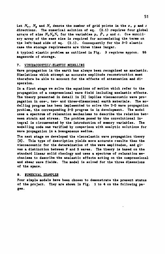
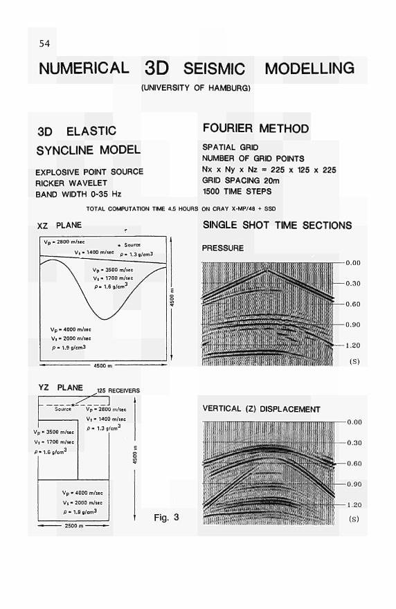
51 Let Nw, Np and Ν, denote the number of grid points in the x, y and ζ directions. The numerical solution of eq. (2.1) requires four global arrays of size ΝτΝ9Ν, for the variables ρ , Ρ, μ and c. One auxili­ary array of the same size is required for accumulating the teras on the left­hand side of eq. (2.1). Consequently for the 3­D elastic case the storage requirements are three times larger. A typical elastic problem as outlined in Fig. 3 requires approx. 95 megaword· of storage.

7. VISCOACOUSTIC/­ELASTIC M0DELLI1G Wave propagation in the earth has always been recognized as anelastic. Simulations which attempt an accurate amplitude reconstruction must therefore be able to account for the effects of attenuation and di­spersion. In a first stage we solve the equations of motion which refer to the propagation of a compressional wave field including anelastic effects. The theory presented in detail in [8] implies viscoacoustic wave pro­pagation in one­, two­ and three­dimensional earth materials. The mo­delling program has been implemented to solve the 2­D wave propagation problem, the corresponding 3­D program is in development. The model uses a spectrum of relaxation mechanisms to describe the relation bet­ween strain and stress. The problem posed by the convolutional in­tegral is circumvented by the introduction of memory variables. The modelling code was verified by comparison with analytic solutions for wave propagation in a homogeneous medium. The next stage we developed the viscoelastic wave propagation theory [9]. This type of description yields more accurate results than the viscoacoustic for the determination of the wave amplitudes, and gi­ves a distinction between Ρ and S waves. The theory is based on the standard linear solid rheology and uses a spectrum of relaxation me­chanisms to describe the anelastic effects acting on the compressional and shear wave fields. The model is solved for the three dimensions of the space.

8. IUMERICAL EXAMPLES Four simple models have been chosen to demonstrate the present status of the project. They are shown in Fig. 1 to 4 on the following pa­ges.

52

NUMERICAL 3D-SEISMIC MODELLING UNIVERSITY OF HAMBURG

t = 0.30 s

SNAPSHOTS — OF PRESSURE WAVEFIELD

3D-ACOUSTIC MODEL

1280 m

MEDIUM

SPECIFICATIONS : FOURIER - METHOD

P-WAVE VELOCITY UPPER LOWER

CONSTANT DENSITY EXPLOSIVE POINT SOURCE RICKER WAVELET (25 Hz) BAND WIDTH 0 - 5 0 Hz 64 * 64x64 GRID ELEMENTS GRID SPACING 20 m

PRESSURE TIME SECTION 0

xtmj

ABSORBING BOUNDARY

j r >à t = 0.35 s

ae Fig. 1 t ime [s]

\

53

NUMERICAL 3D­SEISMIC MODELLING UNIVERSITY OF HAMBURG

3D ­ ACOUSTIC MODEL

440 m

Pressure Snapshot t=300 ms

// \v SPÉCHCATIONS. FOURER­METHOO

P­WAVE VELOCITY:

UPPER 2000 m/l ME DUM

LOWER 4000 ml»

CONSTANT DCNSrrr EXPLOSIVE POUT SOURCE RICKER WAVELET ( 25 Hi ) BAND WOTH 0 . . . SO Hj 84 » 84 » 84 ORD ELEMENTS ORO SPAONQ 20 m

Pressure Snapshot t=350 ms

Pressure Time Section

0Λ0

OSO

0.M

Pressure Snapshot t=400 ms

Fig. 2

54

NUMERICAL 3D SEISMIC MODELLING (UNIVERSITY OF HAMBURG)

3D ELASTIC SYNCLINE MODEL

FOURIER METHOD SPATIAL GRID NUMBER OF GRID POINTS Nx χ Ny χ Nz = 225 χ 125 χ 225 GRID SPACING 20m 1500 TIME STEPS

EXPLOSIVE POINT SOURCE RICKER WAVELET BAND WIDTH 0­35 Hz

TOTAL COMPUTATION TIME 4.5 HOURS ON CRAY X­MP/48 + SSO

XZ PLANE „ SINGLE SHOT TIME SECTIONS Vp ­ 2800 m/sec

Vp V i

Ρ

V i ­ 14

­ 4000 m/iec

­ 2000 m/sec

■ 1.9 g/cm3

00 m/sec

Vp ­ 3500

Vs

P ­

■ 1700

I . 6 9 /

* Source

p « 1.3 g/cm3

m/sec ^ ^

m/sec /

cm3 /

PRESSURE 0.00

— 0.30

0.60

YZ PLANE 125 RECEIVERS

ΖΤΞΠ Source Vp ■ 2800 m/sec

1400 m/sec 3

Vp - 3500 m/sec

Vs - 1700 m/sec

P-1.6g/cm3

Vi

p - 1.3 g/cm'

Vp - 4000 m/sec

Vs - 2000 m/sec

Ρ - 1.9 g/cm3 Fig. 3

VERTICAL (Z) DISPLACEMENT

VISCOELASTIC SEISMIC MODELING (UNIVERSITY OF HAMBURG)

55

70 Rtctivtrs

TWO­DIMENSIONAL MEDIUM RHEOLOQY GENERALIZED STANDARD LINEAR SOLO CONSTANT­Q MEDIA USING TWO SETS OF RELAXATION MECHANISMS FOR EACH PROPAGATING MODE TIME INTEGRATION BEST POLYNOMIAL APPROXIMATION OF THE EVOLUTION OPERATOR IN THE COMPLEX PLANE

SPATIAL DERIVATIVES FOURIER METHOD NUMBER OF GRID POINTS Nx χ Ny ­ 106 χ 106 GRO SPACING 20m

VERTICAL POINT SOURCE RICKER WAVELET PEAK FREQUENCY 20 Hz

SINGLE SHOT TIME SECTIONS

ELASTIC X­OSPLACEMENT

VISCOELASTIC X­OtSPLACEMENT

­2100m

1» Hi) Mil

ÍIO0 1100 JI00 4000

1» Ml) HV»I

1 700 t 700 1 700 laoo

ELASTIC Z­OtSPLACEMENT

VISCOELASTIC Ζ­DISPLACEMENT

i l l l l l l i l l l l i l l l lül i i i i i l i i !« Fig. 4

56

9. REFERENCES [1] Kosloff, D., and Baysal, E., (1982) Forward modelling by the

Fourier­Method, Geophysics,47, 1402 ­ 1412. [2] Kosloff, D., Filho, A.Q., Tessmer, E., and Behle, Α., (1988) Nu­

merical solution of the acoustic and elastic wave equations by a new rapid expansion method (REM), submitted to Geophysical Pro­specting

[3] Tal­Ezer, H., (1986) Spectral methods in time for hyperbolic equations, SIAH J. Numer.Anal., 23, 11 ­ 26.

[4] Kummer, B., Behle, Α., and Dorau, F., (1987) Hybrid modelling of elastic wave propagation in two­dimensional laterally inhomoge­neous media, Geophysics, 52, 765 ­ 771.

[5] Kummer, Β., and Behle, Α., (1988) Fast modelling of seismic wa­ves in laterally inhomogeneous media, submitted to the E8th SEG­meeting, Anaheim, USA.

[6] Kummer, Β., and Behle, Α., (1984) Simulation of transparent boun­daries in finite difference modelling, SEG­meeting, Atlanta, USA.

[7] Kosloff, R., and Kosloff, D., (1986) Absorbing boundaries for wave propagation problems. J.Comp.Phys., Vol.63, 363 ­ 376.

[8] Careione, J.M., Kosloff, D., and Kosloff, R., (1988) Wave pro­pagation simulation in a linear viscoacoustic medium, Geophys. Journal, 93, 2,393 ­ 407.

[9] Care ione, J.H., Kosloff, D., and Kosloff, R., (1987) Wave propa­gation simulation in a linear viscoelastic medium, submitted to Geophysical Journal.