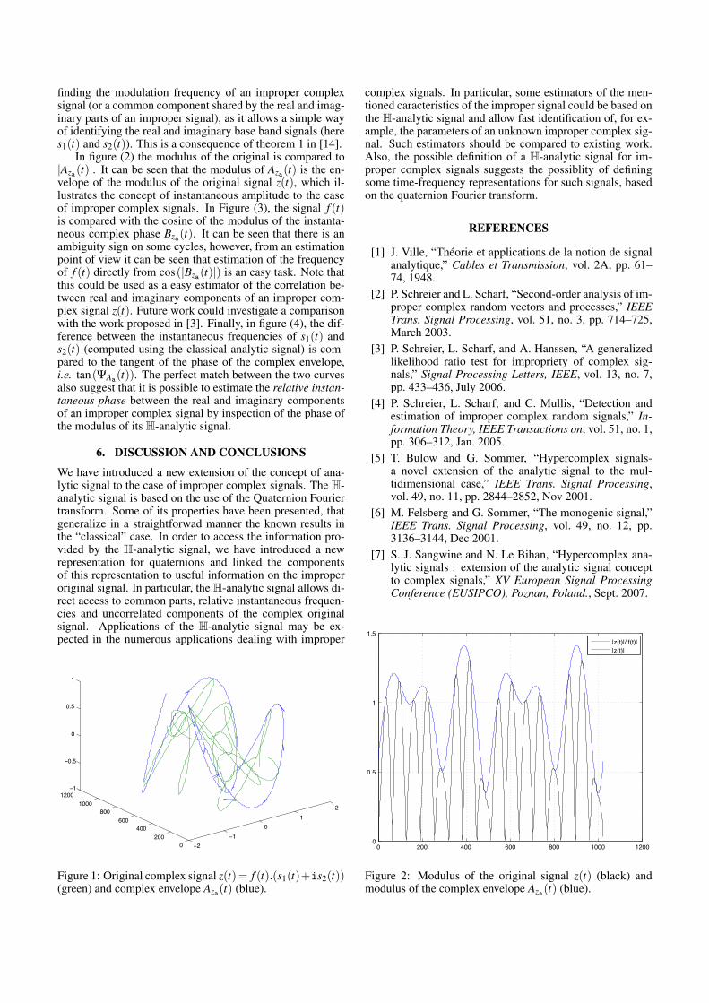
HAL Id: tel-00606665 https://tel.archives-ouvertes.fr/tel-00606665 Submitted on 7 Jul 2011 HAL is a multi-disciplinary open access archive for the deposit and dissemination of sci- entific research documents, whether they are pub- lished or not. The documents may come from teaching and research institutions in France or abroad, or from public or private research centers. L’archive ouverte pluridisciplinaire HAL, est destinée au dépôt et à la diffusion de documents scientifiques de niveau recherche, publiés ou non, émanant des établissements d’enseignement et de recherche français ou étrangers, des laboratoires publics ou privés. Contributions au traitement des signaux à valeurs sur des structures algébriques non-commutatives Nicolas Le Bihan To cite this version: Nicolas Le Bihan. Contributions au traitement des signaux à valeurs sur des structures algébriques non-commutatives. Traitement du signal et de l’image. Université de Grenoble, 2011. <tel-00606665>
Transcript
HAL Id: tel-00606665https://tel.archives-ouvertes.fr/tel-00606665
Submitted on 7 Jul 2011
HAL is a multi-disciplinary open accessarchive for the deposit and dissemination of sci-entific research documents, whether they are pub-lished or not. The documents may come fromteaching and research institutions in France orabroad, or from public or private research centers.
L’archive ouverte pluridisciplinaire HAL, estdestinée au dépôt et à la diffusion de documentsscientifiques de niveau recherche, publiés ou non,émanant des établissements d’enseignement et derecherche français ou étrangers, des laboratoirespublics ou privés.
Contributions au traitement des signaux à valeurs surdes structures algébriques non-commutatives
Nicolas Le Bihan
To cite this version:Nicolas Le Bihan. Contributions au traitement des signaux à valeurs sur des structures algébriquesnon-commutatives. Traitement du signal et de l’image. Université de Grenoble, 2011. <tel-00606665>
ÉCOLE DOCTORALE EEATSSIGNAL, IMAGE, PAROLE ET TÉLÉCOMMUNICATOINS
HABILITATION À DIRIGERLES RECHERCHES
Présentée et soutenue par
Nicolas Le Bihan
Contributions au traitement dessignaux à valeurs sur des
structures algébriquesnon-commutatives
préparée au GIPSA-Lab, Grenoblesoutenue le 20 Juin 2011
Jury :
Rapporteurs : Alfred O. Hero III - University of Michigan, Ann Arbor, USAÉric Moulines - Télécom ParisTech (ENST), ParisPhilippe Réfrégier - Institut Fresnel, Marseille
Président : Olivier J.J. Michel - Grenoble INP, GrenobleExaminateur : Bernard Castaing - ENS, Lyon
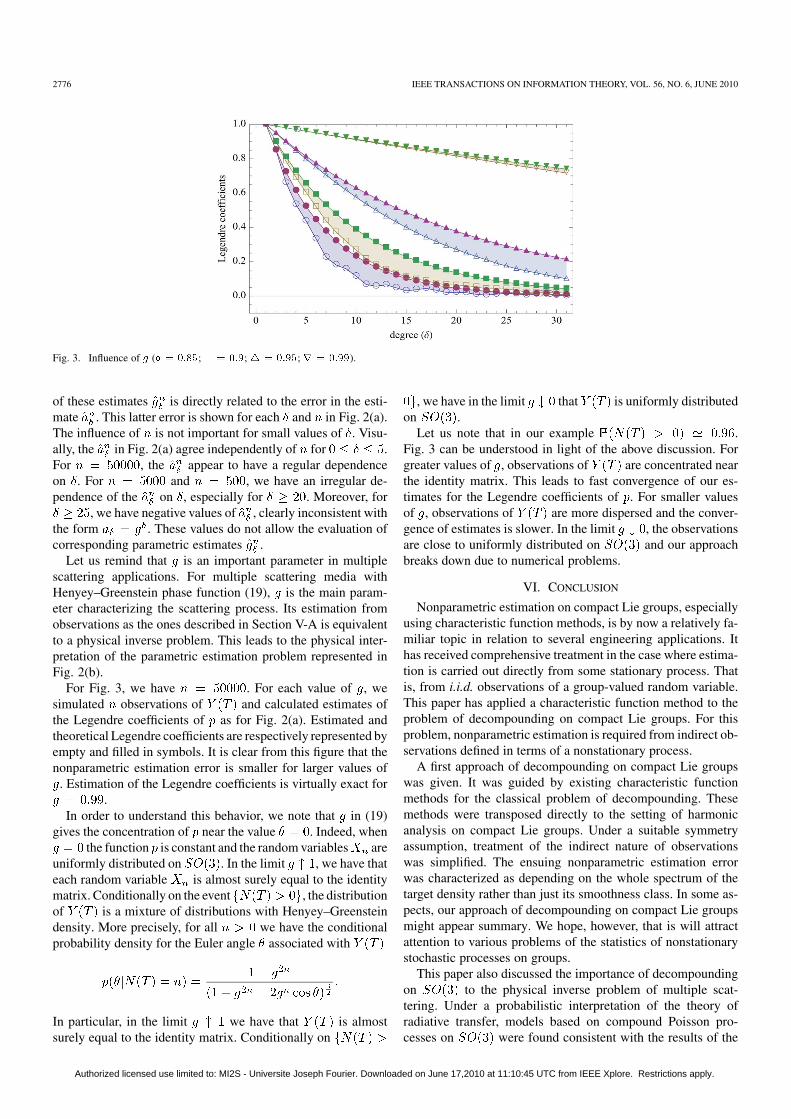
Ce manuscrit présente les travaux de recherche que j’ai menés depuis une dizaine d’an-nées. Il se compose de deux parties distinctes qui possèdent néanmoins un point commun : lanon-commutativité. Les signaux qui sont rencontrés dans ce manuscrit ont tous en communla spécificité de prendre leurs valeurs sur des structures algébriques non-commutatives : qua-ternions, biquaternions, groupes de Lie (groupes matriciels, groupe des rotations), variétésdifférentiables.
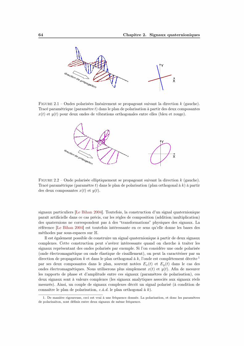
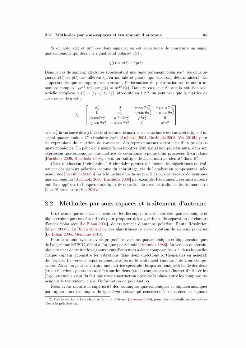
Dans une première partie, je présente les outils de traitement du signal quaternioniquequi vont du traitement d’antenne, à la transformation de Fourier, en passant par l’ex-tension de la notion de circularité. Il est montré comment l’extension quaternionique deces concepts et techniques permet de proposer de nouveaux algorithmes de traitement dessignaux à valeurs quaternioniques ou complexes. La mise au point de ces algorithmes a né-cessité le développement d’outils théoriques nouveaux que nous présentons dans le chapitre1 : décomposition matricielle, circularité des variables aléatoires quaternioniques, représen-tations polaires des quaternions. Dans le chapitre 2, il est montré comment on en arrive àconsidérer des signaux quaternioniques : soit par une modélisation particulière de signauxissus de capteurs vectoriels, soit par transformation de signaux à valeurs complexes. Nousillustrons quelques-uns des résultats obtenus dans le domaine du traitement des signauxquaternioniques, en particulier en traitement d’antenne sismologique et pour l’extension dusignal analytique dans le chapitre 2.
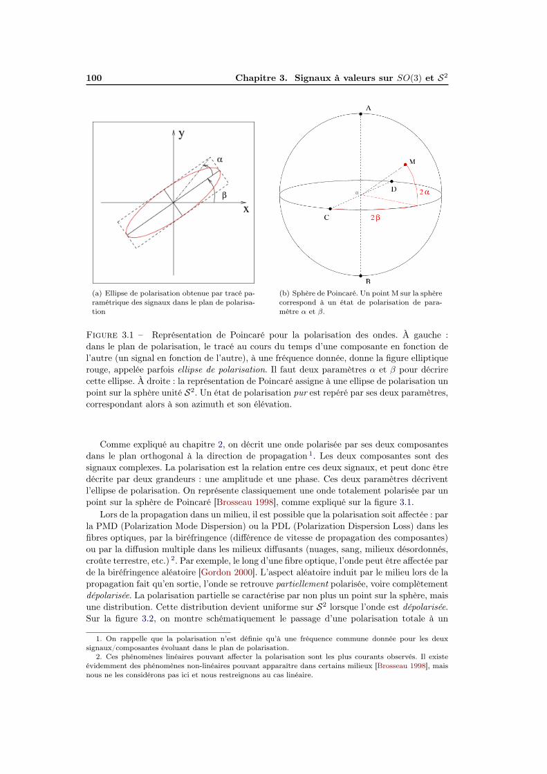
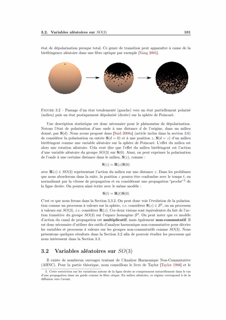
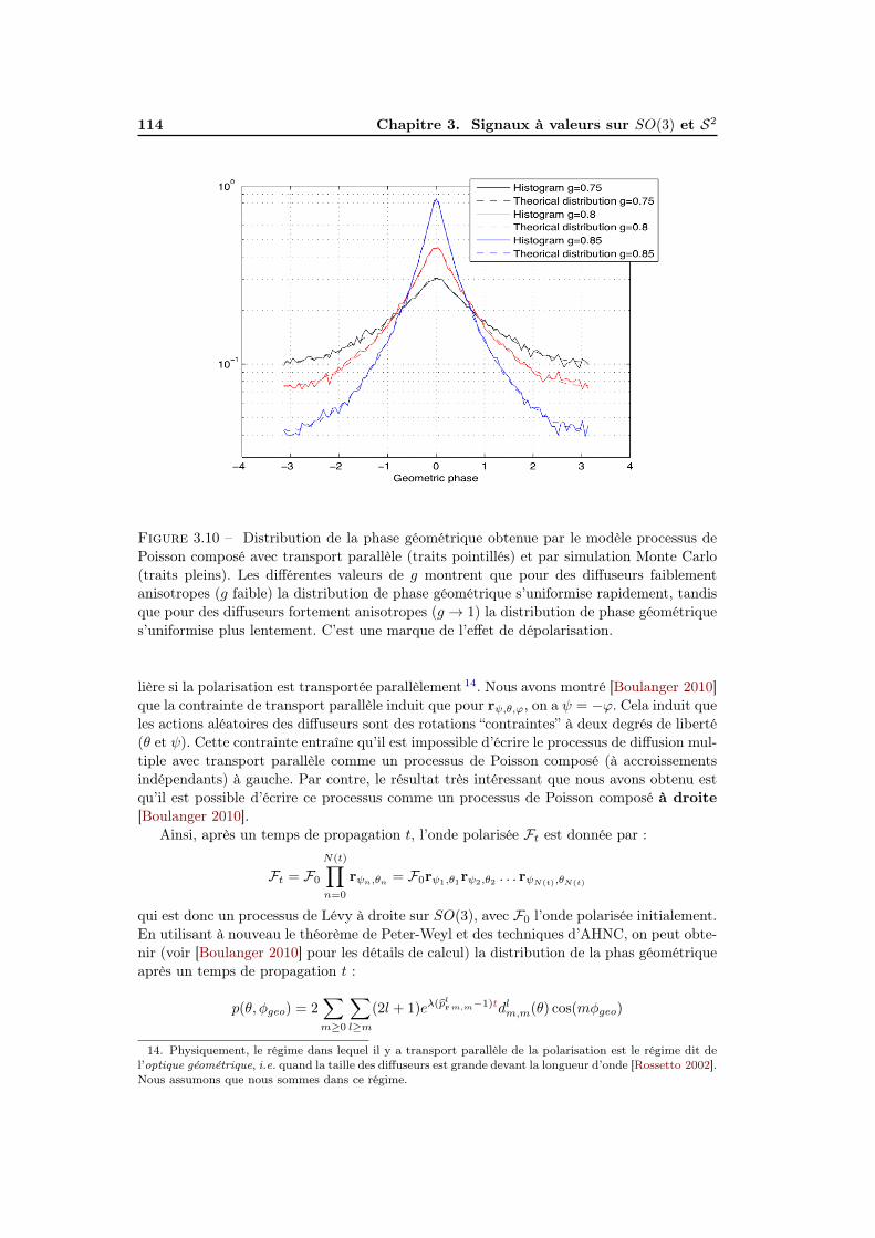
Dans la seconde partie, nous nous intéressons aux signaux qui prennent leurs valeurssur la sphère unité dans R3, i.e. S2, et le groupe des rotations dans l’espace, i.e. SO(3).Les signaux considérés dans cette partie sont les signaux polarisés, et en particulier lessignaux liés aux ondes élastiques. Nous proposons une nouvelle approche pour l’étude dela propagation de ces signaux dans les milieux aléatoires fondée sur les processus de Lévyà valeurs sur le groupe des rotations. Ce modèle nous permet d’étudier les phénomènes dedépolarisation des ondes dans les fibres optiques ou les milieux hétérogènes. L’originalité del’approche proposée permet également un éclairage nouveau sur l’étude de la polarisation,en particulier par une nouvelle définition du degré de polarisation, dite d’ordre supérieur.
Enfin, je présente mes travaux récents sur l’étude de la phase géométrique des ondesélastiques, phénomène dont nous avons rapporté l’observation récemment. Je présente éga-lement un modèle statistique qui prédit l’apparition de cette phase lors de la propagationdes ondes polarisées dans les milieux aléatoires.
Les travaux présentés dans ce manuscrit sont donc de natures diverses, mais ont tous encommun de considérer des signaux et processus dont les échantillons sont à valeurs sur desstructures algébriques non-commutatives. La spécificité de ces signaux fait que leur étuden’est pas très répandue, souvent dispersée, mais leurs champs d’application sont de plus enplus importants. Je présente principalement des techniques de traitement du signal polarisé(sans doute par affinité personnelle), mais les algorithmes qui sont exposés ont un spectrepotentiel d’applications plus large que les seuls signaux polarisés.
1.7.1 "Fundamental representation and algebraic properties of biquater-nions or complexified quaternions” AACA 2010 . . . . . . . . . . . . 18
1.7.2 "Fast Complexified Quaternion Fourier Transform” IEEE TSP 2008 481.7.3 "On Properness Of Quaternion Random Variables” IMA 2004 . . . . 58
Ce premier chapitre présente quelques définitions sur les quaternions ainsi que quelquescontributions qui seront utilisées dans les algorithmes présentés dans le chapitre 2.
Depuis longtemps en traitement du signal, les signaux à valeurs complexes ont oc-cupé une place importante, soit pour décrire l’évolution temporelle du contenu spectrald’un signal monovarié (via le signal analytique [Gabor 1946, Ville 1948] et ses extensions[Hahn 1991, Bulow 2001, Felsberg 2001], soit récement pour étudier des signaux bivariés[Lilly 2010]. Comme souligné régulièrement par les auteurs (en l’occurence par B. Picinbono[Picinbono 1994]), un signal complexe n’est qu’un signal bidimensionnel, mais l’intérêt del’étudier via sa représentation complexe réside dans les outils d’analyse complexe. Un autreavantage, qui a largemant motivé mes travaux utilisant les extensions des complexes, est lefait que les nombres complexes font le lien entre algèbre et géométrie. Ce lien est résumédans la formule d’Euler :
eiθ = cos θ + i sin θ
que Feynmann considérait comme "notre joyau" [Feynman 1963]. Les nombres complexesencodent les transformations géométriques du plan et permettent de les considérer commedes scalaires, plutôt que des matrices. Malgré cela, les signaux complexes sont rarementinterprétés géométriquement, et leur étude est quasi systématiquement conduite via l’étuded’un couple de signaux [Schreier 2010, Lilly 2010].
6 Chapitre 1. Quaternions H
L’idée d’utiliser les quaternions en traitement du signal est venue avec l’introductionde signaux ou images dont les échantillons sont à trois ou quatre dimensions. Dans lespremières tentatives, la géométrie a été mise de côté et l’on a cherché à se soustraire aucas calcul vectoriel en passant par le formalisme des quaternions [Sangwine 1996]. De plusen plus maintenant, l’aspect géométrique est exploité en signal, ce qui rend l’utilisation desquaternions plus pertinente. Cet aspect géométrique (lien avec le groupe des rotations dansR3) a par ailleurs été exploité depuis longtemps en computer graphics [Shoemake 1985].
Un fait particulièrement remarquable est que la formule d’Euler est valable pour lesquaternions. Cela place les quaternions au même rang que les complexes pour faire le lienentre algèbre et géométrie, mais cette fois-ci dans l’espace 3D ou 4D. Avant de présenterquelques aspects des quaternions, notions de base et contributions, rappelons quelques faitshistoriques.
1.1 Historique
Les quaternions ont été découverts en 1843, par Sir William Ronan Hamilton, Physi-cien, astronome et mathématicien irlandais. C’est après une dizaine d’années de tentativesd’extension des nombres complexes à l’espace 3D que Sir W.R. Hamilton réalisa qu’il fallaitquatre dimensions pour construire une algèbre géométrique. Il inventa les quaternions et lafameuse relation entre les trois imaginaires purs. La légende dit qu’il grava cette équationde relation entre les trois imaginaires purs quaternioniques sur le pont de Brougham (aussiappelé pont de Broom) à Dublin. Hamilton développa le calcul pour les quaternions et lesbiquaternions (quaternions à coefficients complexes), mais le calcul vectoriel pris l’ascen-dant sur les quaternions rapidement. Les quaternions ne sont pas tombés dans l’oubli, etleur utilité est reconnue dans plusieurs domaines, entre autre récemment en animation gra-phique [Shoemake 1985, Hanson 2006]. En traitement du signal, si l’on omet leur utilisationpour coder les rotations, ils sont apparus via les transformations de Fourier des images cou-leurs au milieu des années 90 [Sangwine 1996], et depuis ont trouvé quelques applications.Certaines d’entre elles vont être exposées dans ce manuscrit.
Le passage des réels aux complexes fait perdre l’ordonancement (impossible de diresi un complexe est plus grand ou plus petit qu’un autre). Le passage des complexes auxquaternions fait, lui, perdre la commutativité du produit. D’un point de vue purementthéorique, les quaternions sont donc la structure algébrique non-commtative quasiment laplus “simple” sur laquelle on peut commencer à appréhender le traitement du signal non-commutatif. Ce manque de commutativité est une constante dans les travaux présentésdans ce manuscrit et on la retrouvera sur d’autres structures algébriques (qui sont en faitintimement liées aux quaternions) dans la seconde partie du manuscrit.
Il n’est pas vraiment possible de faire une bibliographie complète sur les quaternions. Ilest préférable de se fier à quelques ouvrages de référence. De nombreux ouvrages présententles propriétés des quaternions. Parmi les références les plus complètes, on peut citer le livrede Ward [Ward 1997], celui de Kantor [Kantor 1989] qui présente les quaternions via leurnature hypercomplexe, ou le livre de Girard [Girard 2004] plus orienté vers les formulationsquaternioniques en Physique et le lien avec les algèbres de Clifford. Il existe égalementnombre d’ouvrage présentant le lien entre les quaternions et les groupes de rotations. Uneréférence assez complète sur ce sujet est le livre d’Altman [Altman 1986].
1.2. Définitions et propriétés 7
1.2 Définitions et propriétés
Les quaternions sont des nombres hypercomplexes de dimension 4. L’ensemble des qua-ternions est noté H en l’honneur de Sir W.R. Hamilton. Un quaternion q ∈ H s’écrit, danssa forme Cartésienne, comme :
q = a+ bi + cj + dk (1.1)
avec a, b, c, d ∈ R, et i, j, k des nombres imaginaires purs obéissant aux fameuses 1 relations :
i2 = j2 = k2 = ijk = −1 (1.2)
On en déduit les relations suivantes :
ij = −ji = k (1.3)ki = −ik = j (1.4)jk = −kj = i (1.5)
Le conjugué de q est q = a − bi − cj − dk et son module est |q| =√qq =
√qq = (a2 +
b2 + c2 + d2)1/2. Un quaternion de module égal à 1 est dit unitaire. Pour tout q 6= 0, soninverse est donné par : q−1 = q/|q|2. On dénomme a la partie réelle (ou scalaire) de q,notée Sq et Vq = q − a sa partie vectorielle . De manière évidente, on retrouve la partieréelle par : Sq = (q + q)/2 et la partie vectorielle Vq = (q − q)/2. La conjugaison n’estpas une involution sur H, du fait que ∀q, p on a pq = q p. Il existe tout de même desinvolutions sur H, elles sont de la forme −µqµ, avec µ un quaternion pure unitaire, i.e. uneracine de -1. Parmi toutes ces involutions, trois sont particulières, et permettent d’obtenirles composantes réelles (a, b, c, d) de q par combinaison linéaire comme suit :
a =q − iqi− jqj− kqk
4b =
q − iqi + jqj + kqk
4i
c =q + iqi− jqj + kqk
4jd =
q + iqi + jqj− kqk
4k
La règle d’addition est triviale pour les quaternions, et pour la multiplication, la règleest la suivante, pour p, q ∈ H :
pq = SpSq − Vp.Vq + SpVq + SqVp + Vp ∧ Vq
ou ∧ et le produit vectoriel classique, en considérant les parties vectorielles de p et q commedes vecteurs de R3. La non-commutativité du produit dans H peut se voir ici dans la non-commutativité du produit vectoriel. En complément de ces quelques propriétés, le lecteurpourra consulter par exemple [Ward 1997] pour une liste plus complète des propriétés al-gébriques des quaternions.
1.2.1 Théorèmes de Frobenius et Hurwitz
Sans entrer dans les détails, nous mentionnons ici les théorèmes de Frobenius et Hur-witz 2. Pour une explication particulièrement claire, on consultera les chapitres 17 et 19 de[Kantor 1989]. Ces théorèmes démontrent la place particulière des quaternions (ainsi quecelle des complexes et des octonions). En substance, ces deux théorèmes disent que toute
1. Ces relations auraient été gravées par Sir W.R. Hamilton au matin du 16 octobre 1843, sur le pontde Bourgham à Dublin.
2. Le théorème d’Hurwitz est aussi appelé théorème de Frobenius généralisé.
8 Chapitre 1. Quaternions H
algèbre normée 3 de division 4 est isomorphe à R (réels), C (complexes), H (quaternions) ouO (octonions).
Ces théroèmes motivent l’utilisation des quaternions en traitement des signaux à échan-tillons 3D ou 4D. En effet, il peut s’avérer intéressant de conserver des propriétés liées à lanorme des échantillons qui soient proches de celles connues sur R et C. De plus, l’utilisationd’autres modélisations (algèbres de Clifford, nombres hypercomplexes, bicomplexes) ne ga-rantit pas que tout élément non-nul possède un inverse. Ceci pourrait avoir des conséquenceséventuelles sur la bonne marche de certains algorithmes.
Cette argumentation est éventuellement discutable. En pratique, les conséquences sontinfimes. Malgré tout, l’utilisation des quaternions pour modéliser les échantillons 3D et 4Dparaît plus naturelle du fait de la position exceptionnelle de cette algèbre.
1.2.2 Représentations
En complément de la représentation Cartésienne donnée en (1.1) et de l’expression sca-laire/vectorielle, il est possible de représenter un quaternion de plusieurs manières. Cesreprésentations autorisent pour certaines des interprétations géométriques et d’autres per-mettent d’appréhender le passage entre les complexes (2D) et les quaternions (4D) 5.
Forme polaire : Une propriété remarquable des quaternions est que la formule d’Eulerest toujours valide sur H. Ainsi, tout quaternion q s’écrit :
q = |q| (cos θ + µq sin θ) = |q|eµqθ
avec |q| ∈ R+, µq un quaternion unitaire pure (µ2q = −1) appelé axe de q et θ ∈ [0, 2π[
l’angle de q. L’existence de l’exponentielle quaternionique est due à la convergence de sasérie, qui est possible sur H grâce à l’existence de la norme quaternionique. Il est à noterque le comportement de l’exponentielle sur H est différent de celui connu sur R ou C. Eneffet, d’une manière générale, on a, pour p, q ∈ H non nuls :
eµpθpeµqθq 6= eµpθp+µqθq
C’est une manifestation de la formule de Baker-Campbell-Hausdorff, bien connue en théoriedes groupes de Lie (voir par exemple [Belinfante 1966]).
Forme de Cayley-Dickson : Une façon assez naturelle de voir les quaternions est de lesconsidérer comme des nombres complexes dont les coefficients sont eux-même complexes,mais avec un axe imaginaire orthogonal au premier. Ainsi, on réécrit q comme :
q = z1 + z2j = a+ bi + cj + dk
avec z1 = a + ib et z2 = c + id. On comprend avec cette notation que z1 et z2 sont deuxnombres complexes qui vivent dans deux plans orthogonaux de R4 ne s’intersectant qu’àl’origine. Cette notation est obtenue par un processus de doublement connu dans l’étudedes nombres hypercomplexes [Kantor 1989]. Cette notation est largement utilisée dans lesalgorithmes de traitement du signal et la modélisation des signaux quaternioniques décritsdans le chapitre 2.
3. Une algèbre normée est un corps muni d’une norme ‖.‖ sur lequel on a ‖x‖‖y‖ = ‖xy‖ ∀x, y appar-tenant à ce corps.
4. Une algèbre de division est en fait un corps. En anglais, on parle de “division algebra”.5. Cela s’avère utile lors de la généralisation de techniques/outils de traitement du signal complexe au
cas quaternionique.
1.2. Définitions et propriétés 9
Forme de Cayley-Dickson polaire : Nous avons récemment introduit une nouvellenotation pour les quaternions [Sangwine 2010]. Cette notation a originalement été proposéedans un but d’interprétation du signal hyperanalytique décrit dans le paragraphe 2.3 et dans[Le Bihan 2008]. Tout quaternion q peut d’écrire :
q = AeBj (1.6)
avec A,B ∈ C. A est un module complexe et B une phase complexe. Plus de détails sur cettenotation ainsi que son lien avec celles précédement citées se trouvent dans [Sangwine 2010].
Représentations matricielles : Il est possible (voir par exemple [Ward 1997]) de re-présenter les quaternions par certaines matrices 2× 2 complexes :
H 3 a+ ib+ jc+ kd ∼M =
[a+ ib c+ id
−c+ id a− ib
]=
[z1 z2−z∗2 z∗1
]∈M2×2(R)
avec z1 et z2 issus de la notation de Cayley-Dickson. Cette notation matricielle permetd’intuiter le lien particulier entre les quaternions unitaires (i.e. q ∈ H t.q. |q| = 1) et legroupe spécial unitaire SU(2) (voir [Altman 1986]).
Représentations vectorielles : Les quaternions étant des nombres 4D, il est égalementpossible de les considérer comme des vecteurs de dimension 4. Cette notation a été utiliséedans l’étude de la circularité des variables aléatoires quaternioniques [Amblard 2004]. Ilexiste principalement trois représentations pour un quaternion q ∈ H :
– Réelle : qR = [a b c d]t
– Complexe : qC = [z1 z∗1 z2 z
∗2 ]t
– Quaternionique qH =[q qi qj qk
]tOn peut donc voir un quaternion alternativement comme un vecteur de R4, de C4 ou de H4.Cette façon d’appréhender les quaternions est similaire à la repésentation dite de "vecteuraugmenté" utilisée en traitement des signaux complexes [Schreier 2010].
1.2.3 Géométrie
La faculté des quaternions a représenter les transformations géométriques en 3D est unfait connu depuis longtemps. Ils ont été utilisés dans de nombreux domaines (animation[Shoemake 1985], aéronautique [Kuipers 1999]) et la description de leur lien avec le groupedes rotations est décrite dans de nombreux ouvrages (par exemple [Altman 1986]). Nousprésentons quelques résultats bien connus sur les transformations géométriques à l’aidedes quaternions. Pour un inventaire plus exhaustif, nous renvoyons à [Coxeter 1946] et[Ward 1997].
Rotations en 3D Étant donné un point P dans l’espace tridimensionnel, représenté parle quaternion p = xi + yj + zk, alors pRq
donné par :
pRq= q−1pq
avec q = cosθ+µ sin θ un quaternion unitaire (i.e. |q| = 1), est le point obtenu par rotationdu vecteur p autour de µ d’un angle 2θ. Un quaternion pur peut être vu alternativementcomme un vecteur ou un point de R3. Attention tout de même car rigoureusement c’est unbivecteur.
10 Chapitre 1. Quaternions H
Rotations en 4D Étant donné un point P de l’espace 4D, représenté par un quaternionp = s+ xi + yj + zk, alors la transformation suivante :
pRab= apb
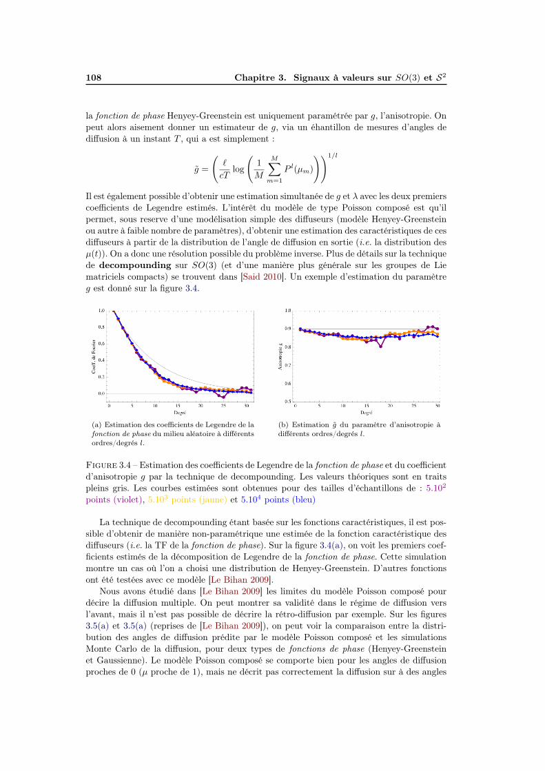
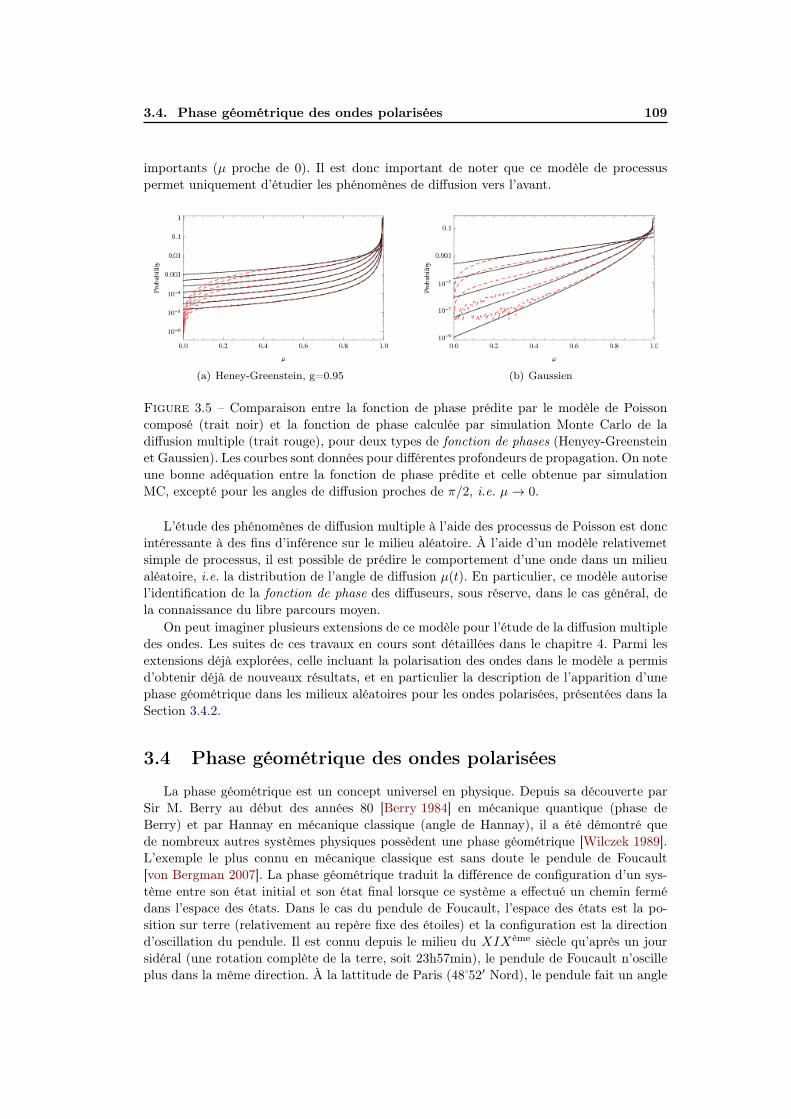
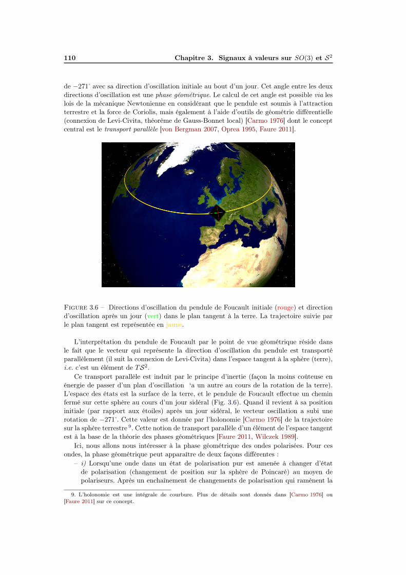
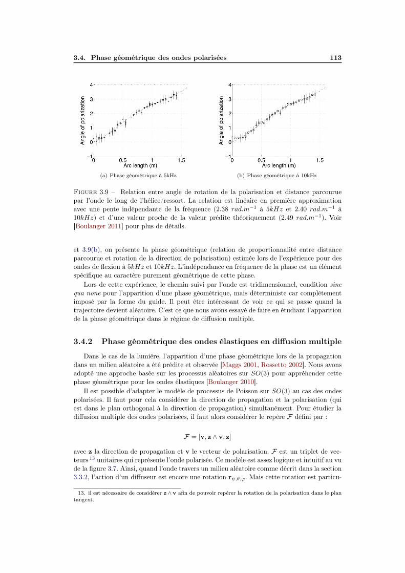
avec a ∈ H et b ∈ H deux quaternions unitaires, est une rotation de p autour du plan définipar les parties vectorielles de a et b.
Translation de Clifford Étant donné un point de R4, noté P et représenté par le qua-ternion p = s+ xi + yj + zk, la transformation suivante :
pT ga
= ap
avec a ∈ H un quaternion unitaire, est une translation de Clifford à gauche. On définitde même une translation à droite comme pT g
a= pa. Géometriquement, la translation de
Clifford consiste en une rotation simultanée d’un même angle (si a = eηϕ cette rotation estd’angle ϕ), et dans deux plans distincts de R4, définis par les deux nombres complexes quiforment le quaternion q 6.
Les quaternions, tout comme les complexes en 2D, représentent des transformationsgéométriques par des opérations algébriques sur des scalaires, évitant ainsi de recourir àl’usage des matrices. Ceci a des conséquences, en particulier en stabilité numérique dansl’accumulation des rotations.
1.2.4 H et les groupes SU(2) et SO(3)
Comme nous venons de le voir, les quaternions permettent d’écrire de manière conciseles transformations géométriques dans R3 (ainsi que dans R4). En fait, le lien entre les qua-ternions et le groupe des rotations est bien connu [Altman 1986]. Les quaternions unitairessont isomorphes à SU(2), le groupe des matrices complexes de déterminant égal à 1 et uni-taires. On peut se convaincre de cet isomorphisme en rematquant l’isomorphisme entre leséléments de base des quaternions, i.e. 1, i, j et k, et les matrices de Pauli [Altman 1986].
Pour SO(3), chaque élément de ce groupe est en correspondance avec deux quater-nions unitaires, +q et −q. Cet homomorphisme entre SO(3) et SU(2) est bien connu, avecquelques implications amusantes comme le “belt trick” [Hanson 2006] qui traduit le fait qu’ilfaut “deux copies de SU(2) pour recouvrir SO(3)”.
Nous n’utiliserons pas dans ce chapitre cette correspondance entre quaternions unitaireset le groupe des rotations SO(3), mais ce lien permet de voir les connexions possibles entreles deux parties de ce manuscrit.
1.2.5 Quaternions complexes, octonions et algèbres de Clifford
Parmi les généralisations à la dimension 8 des nombres hypercomplexes, nous en men-tionnons ici deux.
Les biquaternions HC sont construits par la procédure de doublement. Cela revient à“complexifier” les coefficients d’un quaternion q ∈ H comme défini dans l’équation 1.1. Ainsiles coefficients a, b, c et d d’un biquaternion sont des complexes, avec pour nombre imagi-naire I (par exemple a = <(a) + I=(b)), et évidement I2 = −1. Le nombre imaginaire Icommute avec tous éléments de la base canonique de H, i.e. Ii = iI, Ij = jI et Ik = kI.Comme le prédit le théorème de Frobenius, les biquaternions ne forment pas une algèbre
6. Dans la translation de Clifford du quaternion q, les deux partie de a décomposition de Cayley-Dicksonde q vont être “tournées” est fonction de l’axe de la translation de Clifford.
1.3. Matrices de quaternions 11
normée de division. En fait, il existe des biquaternions non-nuls dont la norme est 0 (divi-seurs de zéros) et la norme d’un produit de biquaternions n’est pas le produit des normes 7
des biquaternions. L’article [Sangwine 2011] qui est inclus dans la section 1.7 fait un étatde l’art des propriétés des biquaternions.
Les octonions O sont les nombres hypercomplexes de dimension 8 qui possèdent lespropriétés intéressantes vis à vis de la norme (définie de manière standard). Malheureuse-ment, ils souffrent d’un problème assez important, ils ne sont pas associatifs par rapport auproduit, i.e. (ab)c 6= a(bc) pour a, b, c ∈ O en général. Quelques utilisations des octonionsexistent, principalement en Physique théorique (formulation octonionique en électrodyna-mique par exemple [Lounesto 2001]). On peut dire que si les octonions n’ont pas trouvéd’applications en traitement du signal, c’est sans doute parce qu’ils ne possèdent pas dereprésentation matricielle (une représentation matricielle est forcement associative). Ceciexplique que la TF octonionique, entre autre, ne peut être obtenue via une repésentationmatricielle réelle, complexe ou quaternionique.
Les limitations des nombres hypercomplexes dans les dimensions “élevées” sont peut-êtrele signe que la solution se trouve du côté des algèbres de Clifford (parfois appelées également“algèbres géométriques”). Plusieurs ouvrages présentent des applications de ces algèbres entraitement des images et en robotique [Sommer 2001], et il est sans doute possible d’utiliserces algèbres en traitement du signal (1D, à échantillons multivariés). Ce point sera abordéde nouveau dans les perspectives de mes travaux liés au signal hyperanalytique et presentédans la section 2.3.
1.3 Matrices de quaternions
La non-commutativité des quaternions induit quelques difficultés dans l’étude des ma-trices de quaternions. Les matrices de quaternions ont été étudiées depuis le milieu duXXeme siècle [Wolf 1936, Lee 1949, Brenner 1951] et il existe toujours une activité de re-cherche sur le sujet [Wu 2008]. L’article de référence est celui de F. Zhang [Zhang 1997] quifait une synthèse des résultats théoriques connus à l’époque. À titre d’exemple, on men-tionne ici deux concepts très connus dans l’étude des matrices qui se compliquent lors dupassage à H : 1) les valeurs propres d’une matrice quaternioniques peuvent être droites ougauches [Zhang 1997] ; 2) le calcul du déterminant d’une matrice dépend du sens de par-cours des éléments. Le problème 1) est lâchement évité 8 dans ce manuscrit, car nous neparlons que de valeurs propres droites (les seules pour lesquelles la théorie est bien établieà ce jour). Dans le cas du déterminant, plusieurs définitions existent, par exemple, nouscitons celle de J. Dieudonné [Dieudonné 1943].
Singular Value Decomposition (SVD) L’existence de la SVD pour une matrice dontles éléments sont des quaternions est connue depuis un certain temps [Zhang 1997]. Ainsi,tout matrice A ∈MN×M (H) peut s’écrire :
A = U∆Vt
avec U ∈ MN×N (H) et V ∈ MM×M (H) deux matrices unitaires et ∆ ∈ MN×M (R) unematrice diagonale réelle. En 2001, nous avons proposé un algorithme de calcul de cette SVD
7. Il est à noter que la définition de la norme pose problème également pour les biquaternions. Voir[Ward 1997, Sangwine 2011]
8. ou habilement contourné, selon le point de vue ...
12 Chapitre 1. Quaternions H
[Le Bihan 2004], se basant sur la matrice adjointe, notée χA9, de la matrice quaternionique
A.En 2006 et 2007, nous avons proposé avec S.J. Sangwine, deux nouveaux algorithmes
en arithmétique quaternionique pour le calcul de cette décomposition [Sangwine 2006,Le Bihan 2007b]. L’approche algorithmique purement quaternionique permet d’atteindreune précision plus importante dans le calcul des valeurs singulières et nécessite moins d’opé-rations arithmétiques, réduisant ainsi le coup de calcul. Ces deux algorithmes sont basés surdes extensions quaternioniques des transformations de Householder [Bunse-Gerstner 1989]et de Givens [Janovská 2003].
Eigenvalue decomposition (EVD) Comme précisé auparavant, nous parlons ici desvaleurs propres droites, c’est à dire les λ t.q. Aλ = vλ avec A ∈ MN×N (H) et v ∈ HN .Plus de détails sur ces valeurs propres se trouvent dans [Zhang 1997]. Ici, nous mentionnonsla contribution que nous avons apporté à l’étude des valeurs propres des matrices de biqua-ternions (quaternions à coefficients complexes). Nous avons proposé un algorithme de calculdes valeurs propres d’une matice de biquaternions Hermitienne à l’aide d’une technique dematrice adjointe quaternionique [Le Bihan 2007a].
Matrices polynomiales Quelques résultats sont connus pour les polynômes de quater-nions, et en particulier pour le calcul des zéros de ces polynômes [Serôdio 2001]. Dansla continuité des résultats de diagonalisation des matrices quaternioniques et biquaternio-niques, nous avons proposé un algorithme de diagonalisation pour les matrices polynomialesquaternioniques [Le Bihan 2005]. Il est ainsi possible de montrer qu’une matrice polyno-miale quaternionique A[z] ∈MN×N (H[z]) de degré p, donnée par :
A[z] =
p−1∑
l=0
Alzl = A0 + A1z + A2z
2 + ...+ Ap−1zp−1 (1.7)
avec Aα ∈MN×N (H) ∀α et z = <(z) + I=(z) ∈ C, peut être diagonalisée dans le cas para-hermitien (voir les détails dans [Le Bihan 2005]). L’algorithme que nous avons proposépour cette diagonalisation est basé sur les transformations de Givens quaternioniques. Cetalgorithme a été utilisé à des fins de séparation de mélanges convolutifs d’ondes polarisées[Le Bihan 2005, Menanno 2010].
1.4 Transformation de Fourier quaternionique
L’idée de définir une Transformée de Fourier Quaternionique (TFQ), ou hypercomplexe,est apparue à plusieurs auteurs, et vraisemblablement de manière indépendante, dans desdomaines de recherche distincts. En 1987-88, une TF hypercomplexe (bicomplexe en fait)est introduite pour le traitement des données RMN 2D [Ernst 1987, Delsuc 1988]. Cettetransformée a été introduite afin de séparer des fréquences de rotation de spins en RMN.
La transformation de Fourier quaternionique a ensuite été redécouverte en 1992 parTodd A. Ell dans un autre contexte. Il avait pour objectif de procurer un équivalent à latransformée de Fourier dans le cas de systèmes bilinéaires invariants dans le temps. Il aainsi pu proposer une description en gain-phase de ces systèmes [Ell 1992, Ell 1993].
En 1996, S.J. Sangwine a proposé une transformation de Fourier 2D pour les imagescouleurs, i.e. pour les signaux bidimensionnels à échantillons vectoriels (chaque pixel RGB
9. La matrice matrice adjointe d’une matrice quaternionique A ∈ MN×M (H) est une matrice χA ∈M2N×2M (C), à valeurs complexes, dont les propriétés peuvent être reliées à celle de A, voir [Zhang 1997,Le Bihan 2004] pour plus de détails
1.4. Transformation de Fourier quaternionique 13
est représenté par un quaternion pur) [Sangwine 1996]. S.J. Sangwine a ensuite beaucouptravaillé sur les différentes définitions des TF 2D quaternioniques, établissant le lien entre lesdifférentes définitions possibles (gauche, droite, bilatérale) 10. Bien que sa définition originalede la TFQ 2D soit bilatérale [Ell 1993, Sangwine 1996], S.J. Sangwine a principalementtravaillé depuis sur les TFQ unilatérales et leur interprétation dans l’étude des imagescouleurs. La TFQ unilatérale droite d’un signal bivarié s(x, y) : R×R→ H est donnée par :
Sµ(ν, ω) = TFQµ [s(x, y)] =
∫ +∞
−∞s(x, y)e−2πµ(νx+ωy)dxdy
avec µ un quaternion pure unitaire. On remarque tout de suite qu’il existe une infinité dedéfinitions possibles du fait du choix possible de µ. En pratique, pour les images couleurs,le choix de µ n’a pas beaucoup d’importance. On verra plus tard qu’il est plus contraintdans le cas de TFQ 1D.
Au début des années 2000, l’équipe de G. Sommer à Kiel, sous l’impulsion de T. Bulöw,s’est intéressée à l’extension du signal analytique au cas des images (signaux 2D), en utilisantla TFQ. Une bonne synthèse de leurs travaux se trouve dans le livre édité par Sommer[Sommer 2001]. Les travaux de Bulöw sont basés sur une TFQ bilatérale très similaire àcelle de T.A. Ell [Ell 1992] et s’intéressent à proposer une TFQ pour des images dont lespixels sont à valeurs réelles. Ainsi, la TFQ bilatérale de s(x, y) : R × R → R est donnéepar :
S(ν, ω) =
∫ +∞
−∞e−2πjνxs(x, y)e−2πkωydxdy
L’utilisation de cette transformée pour la définition d’un signal analytique 2D conduità la définition de plusieurs phases exploitables dans le cas de signaux 2D séparables[Bulow 2001]. On notera que Bulow utilise dans ses travaux un triplet de phases 11 quisont liées aux angles d’Euler, ce qui revient à utiliser encore une autre représentation desquaternions (voir [Bulow 2001]).
Depuis la publication de tous ces résultats sur les TFQs 2D, quelques applications ont étéproposées pour ces algorithmes. Encore une fois, sans vouloir être exhaustif, on peut citerpar exemple : l’analyse d’images [Ell 2007], l’estimation de mouvement [Alexiadis 2009], lewatermarking [Bas 2003] ou la détection en sonar [Redfield 2002], etc.
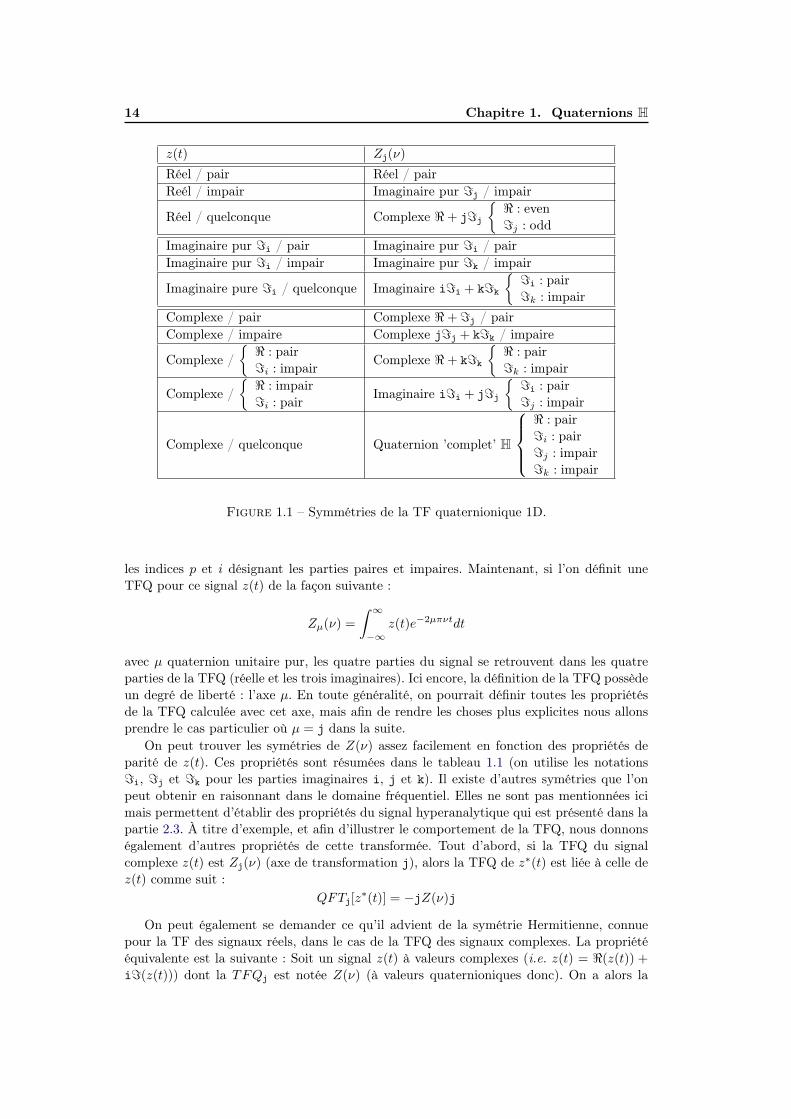
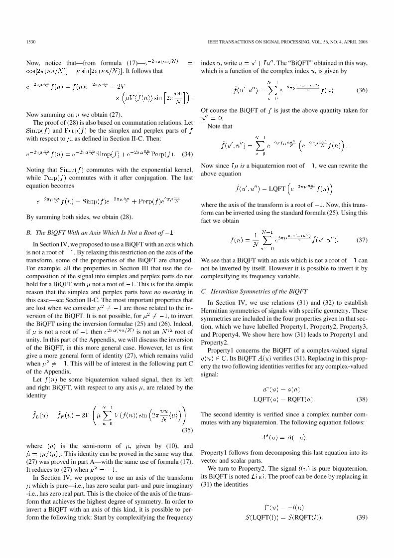
L’idée que nous avons avancée avec S.J. Sangwine en 2006 est différente. Nous avonsentrepris de définir une transformation de Fourier Quaternionique pour des signaux à valeurscomplexes 1D. L’idée de base est en fait la même que celle développée en RMN ou dansles travaux de T. Bulöw, elle consiste à séparer les symétries du signal dans des partiesimaginaires de la transformée. Dans le cas complexe 1D, on sait que la transformée deFourier (complexe) d’un tel signal ne satisfait plus la symétrie hermitienne (S∗(ν) = S(−ν))quand le signal complexe est "quelconque” (parties réelles et imaginaires possédant unepartie paire et une partie impaire). Ainsi, un signal complexe z(t) peut s’écrire d’une manièregénérale :
z(t) = [<(z(t))p + <(z(t))i] + i [=(z(t))p + =(z(t))i]
10. La non-commutativité des quaternions rend possible la définition de plusieurs TF, selon que le noyaude la transformée est à gauche, droite, ou que deux noyaux (à gauche et droite) soient utilisés. On consultera[Ell 2007] pour un état de l’art récent et l’équivalence entre les différentes transformations 2D possibles.11. En fait, il existe encore une autre notation de type “polaire” pour les quaternions. On peut écrire
q ∈ H comme : q = ‖q‖ exp(iϕ) exp(iθ) exp(iψ). Nous n’utiliserons pas cette notation dans ce manuscrit,mais il pourrait être intéressant d’essayer de l’appliquer dans l’interprétation du signal hyperanalytiquedécrit dans la section 2.3.
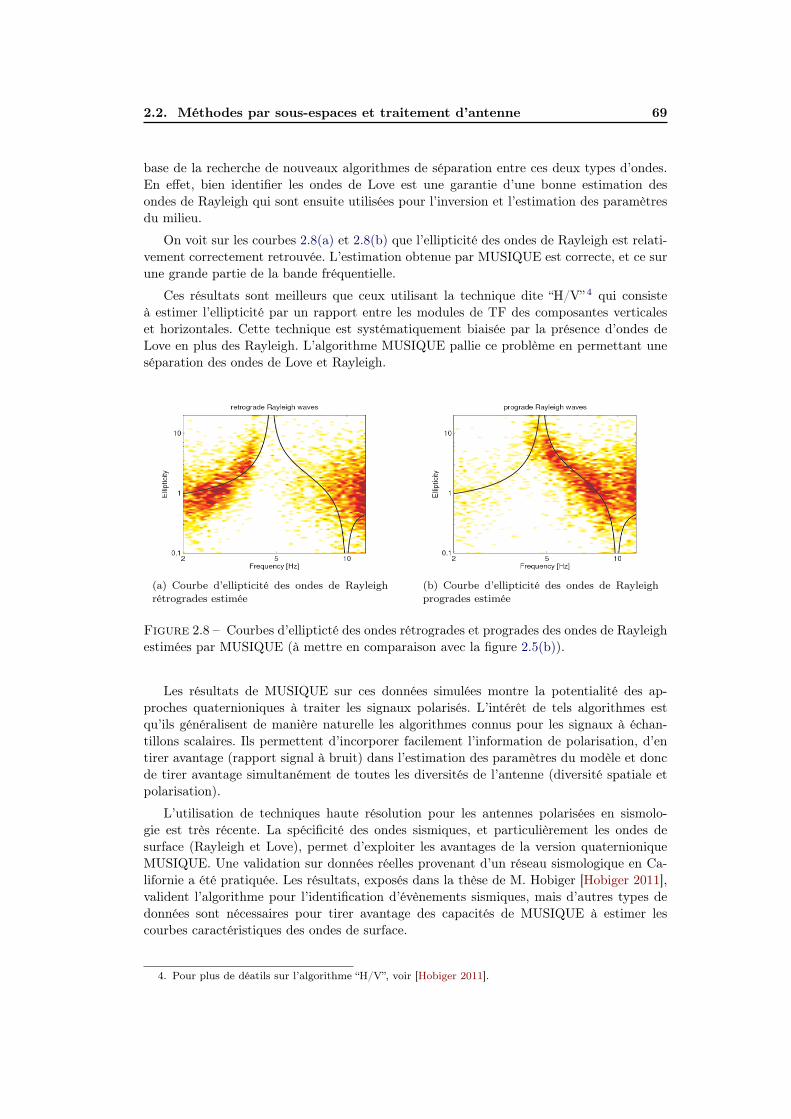
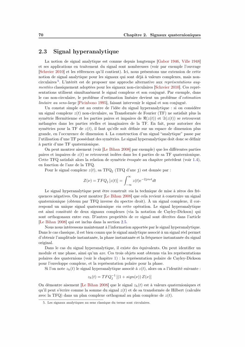
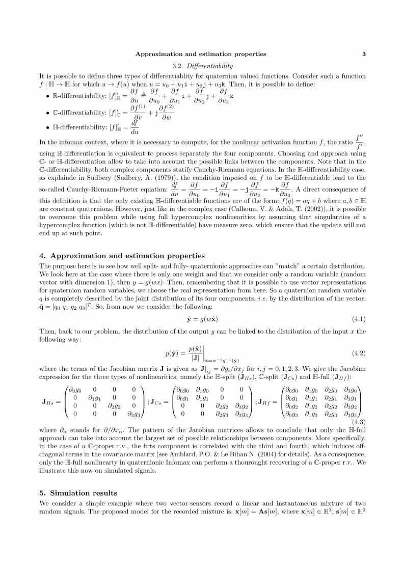
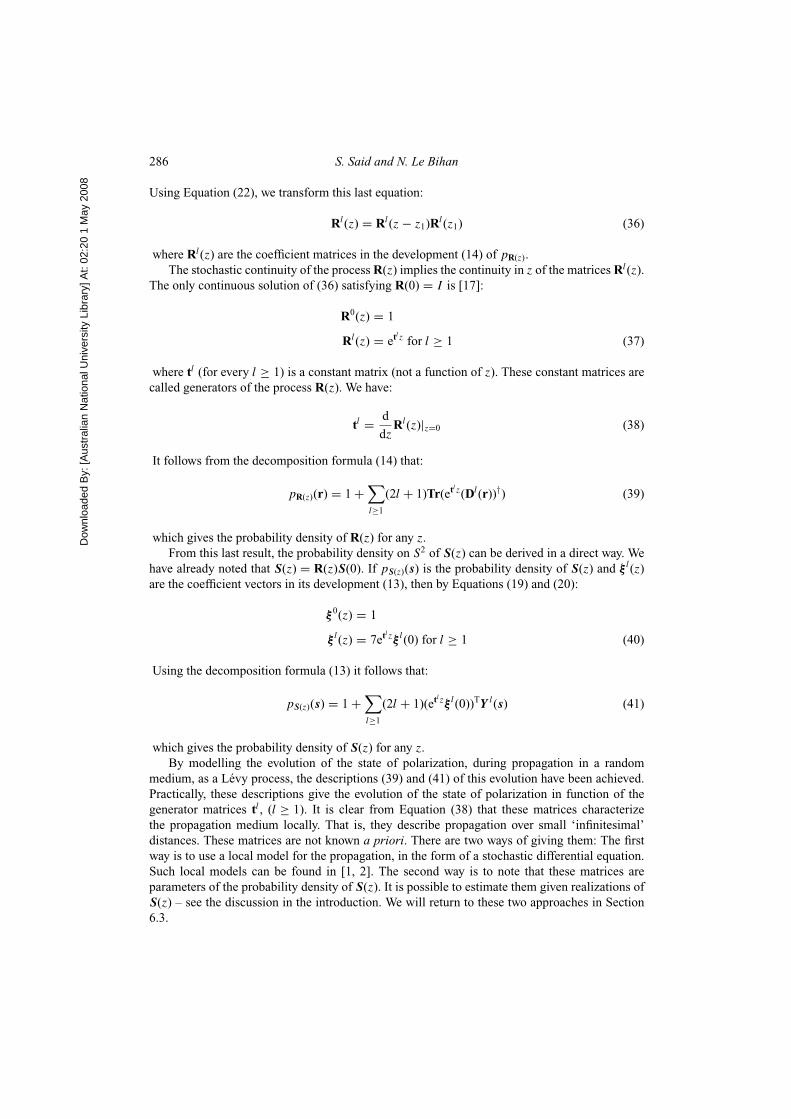
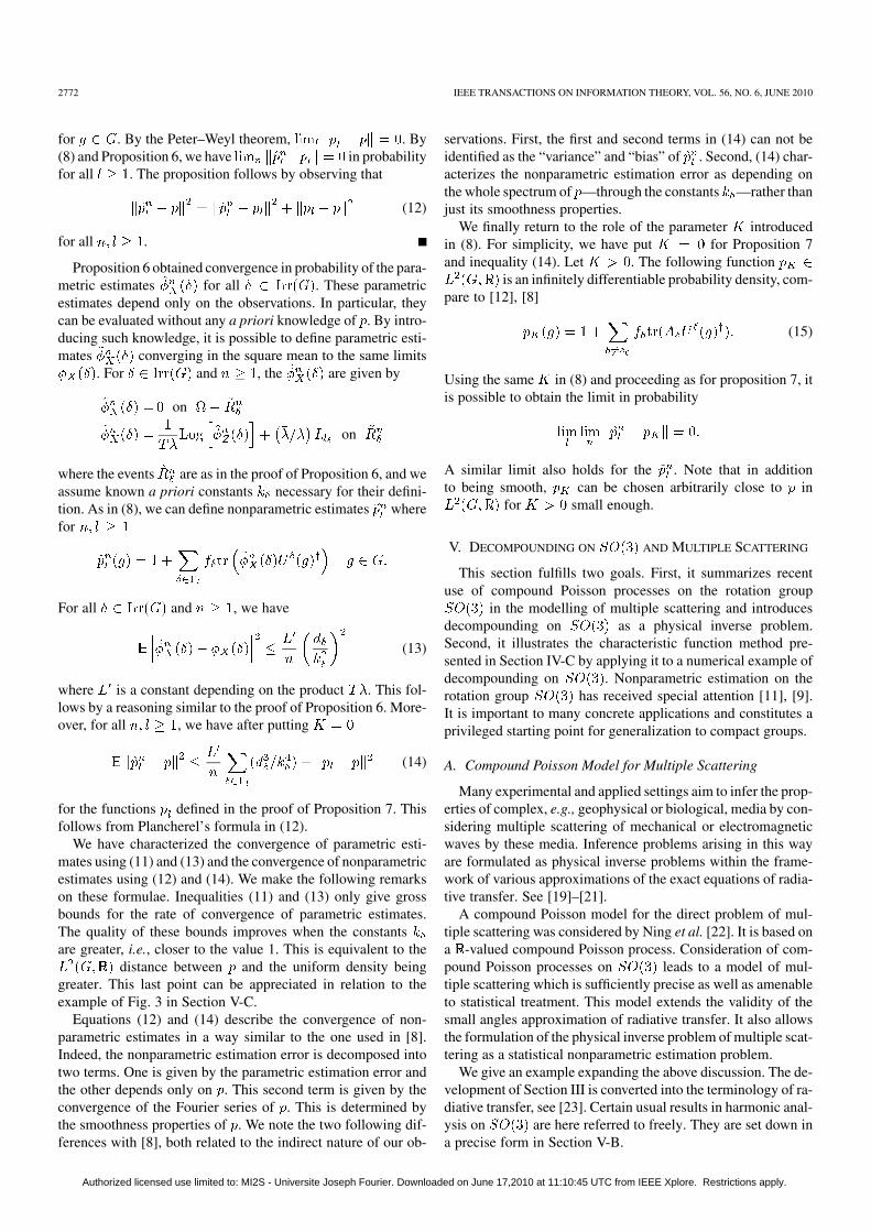
Figure 1.1 – Symmétries de la TF quaternionique 1D.
les indices p et i désignant les parties paires et impaires. Maintenant, si l’on définit uneTFQ pour ce signal z(t) de la façon suivante :
Zµ(ν) =
∫ ∞
−∞z(t)e−2µπνtdt
avec µ quaternion unitaire pur, les quatre parties du signal se retrouvent dans les quatreparties de la TFQ (réelle et les trois imaginaires). Ici encore, la définition de la TFQ possèdeun degré de liberté : l’axe µ. En toute généralité, on pourrait définir toutes les propriétésde la TFQ calculée avec cet axe, mais afin de rendre les choses plus explicites nous allonsprendre le cas particulier où µ = j dans la suite.
On peut trouver les symétries de Z(ν) assez facilement en fonction des propriétés deparité de z(t). Ces propriétés sont résumées dans le tableau 1.1 (on utilise les notations=i, =j et =k pour les parties imaginaires i, j et k). Il existe d’autres symétries que l’onpeut obtenir en raisonnant dans le domaine fréquentiel. Elles ne sont pas mentionnées icimais permettent d’établir des propriétés du signal hyperanalytique qui est présenté dans lapartie 2.3. À titre d’exemple, et afin d’illustrer le comportement de la TFQ, nous donnonségalement d’autres propriétés de cette transformée. Tout d’abord, si la TFQ du signalcomplexe z(t) est Zj(ν) (axe de transformation j), alors la TFQ de z∗(t) est liée à celle dez(t) comme suit :
QFTj[z∗(t)] = −jZ(ν)j
On peut également se demander ce qu’il advient de la symétrie Hermitienne, connuepour la TF des signaux réels, dans le cas de la TFQ des signaux complexes. La propriétééquivalente est la suivante : Soit un signal z(t) à valeurs complexes (i.e. z(t) = <(z(t)) +
i=(z(t))) dont la TFQj est notée Z(ν) (à valeurs quaternioniques donc). On a alors la
1.5. Circularité 15
relation suivante par calcul direct :
X(ν) = −iX(−ν)i
On voit ainsi que dans le cas des TFQ, c’est l’involution dont l’axe est le même que celuide la transformation qui joue le rôle de la conjugaison dans le cas “classique” 12.
Finalement, on peut tenter de réécrire l’identité de Parseval dans le cadre des TFQ.Étant donnés x(t) et y(t) deux signaux complexes, et leurs TFQj notées X(ν) et Y (ν),alors l’égalité suivante est vérifiée :
∫ +∞
−∞x(t)y∗(t)dt =
∫ +∞
−∞X(ν) (−jY (ν)j) dν
On démontre aisement cette égalité avec la propriété de la TFQ de y∗(t) donnée précéde-ment.
Ces propriétés illustrent les spécificités du calcul impliquant la TFQ et montrent l’im-portance des involutions dans l’étude de cette transformée. On gardera à l’esprit égalementque la non-commutativité du produit des TFQ rend leur manipulation délicate et qu’un soinparticulier doit être apporté à l’ordre des produits. Toutefois, une étude systématique de laTFQ 1D reste encore à être menée. Une étude complète n’existe pas à l’heure actuelle. Cetteétude fait partie de mes perspectives. Dans nos travaux, nous avons utilisé cette transfor-mée afin de définir des grandeurs instantanées pour les signaux complexes non-stationnairesnon-circulaires. Ce travail est présenté dans la section 2.3 et illustre l’intérêt de la TFQ dansl’étude des signaux complexes non-circulaires.
Enfin, on peut se demander comment étendre ces résultats obtenus pour la transforméede Fourier Quaternionique à des dimensions supérieures. Plusieurs solutions existent, et nousavons travaillé sur une extension à la dimension 8 : la TF Biquaternionique [Said 2008b].Nous avons étudié cette transformation et montré son intérêt pour l’étude des signaux àéchantillons vectoriels 4D. Les détails sont dans l’article inclus dans la section 1.7. On peutévidement se poser la question de la généralisation de ces transformées hypercomplexesaux dimensions supérieures à 8. Les travaux que nous avons mené depuis quelques annéesmontrent que l’aspect géométrique qu’apportent les transformées quaternioniques est cen-tral. Si cet aspect est accessible en dimension 4 ou 8, au delà, c’est moins évident. Il mesemble qu’une théorie plus générale doit pouvoir être établie en se basant sur les algèbresde Clifford [Sommer 2001]. Les transformations de Fourier de Clifford existent est doiventpermettre de mener le même type d’analyse que celles quaternioniques que nous avons me-nées, mais pour n’importe quelle dimension N . L’étude de ces transformées en traitementdes signaux est une des perspectives de ces travaux.
1.5 Circularité
La notion de circularité pour les variables aléatoires et les signaux complexes est bienconnue en traitement du signal. Elle a donné lieu à un grand nombre de publications depuisles premiers travaux dans le domaine du signal par B. Picinbono [Picinbono 1994]. Lecas circulaire est finalement assez simple et beaucoup des travaux récents s’intéressent enparticulier au cas non-circulaire 13. Ne pouvant être exhaustif, nous renvoyons à l’ouvrage
12. En fait, la conjugaison est une involution sur C, alors qu’elle ne l’est pas ( !) sur H. La symétrieHermitienne est donc liée aux involutions sur l’espace considéré et s’étend donc au cas quaternionique viacelles-ci.
13. On rappelle qu’une variable aléatoire complexe z est dite circulaire au sens large si z d= zeiθ pour
tout θ ∈ R. La conséquence est que la partie réelle et la partie imaginaire de z sont décoréllées et de mêmevariance.
16 Chapitre 1. Quaternions H
récent [Schreier 2010] et les références s’y trouvant. Ce livre présente une synthèse destravaux dans le domaine.
Dans le cas des quaternions, la notion de circularité a tout d’abord été introduite parN.N. Vakhania [Vakhania 1998]. En 2004, nous avons généralisé la définition de Vakhania[Amblard 2004] pour la circularité des variables aléatoires quaternioniques. Ainsi, pour unevariable aléatoire quaternionique q, il existe deux niveaux de circularité : la Cη-circularitéet la Hη-circularité. Ainsi, une variable aléatoire quaternionique q est dite Cη-circulaire si :
qd= eηϕq, ∀ϕ
pour un et un seul quaternion unitaire pur η = i, j ou k (quand q est exprimé dans la basequaternionique classique 1, i, j, k ). Une variable aléatoire quaternionique q sera dite Hη-circulaire si la même égalité est vérifiée quelque soit le quaternion pur η. On remarquera quedans le cas quaternionique, il ne s’agit pas d’une invariance par rotation de la distributionde q pour la Cη-circularité, mais une invariance par translation de Clifford à gauche.
La différence majeure entre le cas complexe et le cas quaternionique est donc qu’ilexiste deux niveaux de circularité sur H. Ces niveaux de circularité se répercutent surla matrice de covariance de la variable q dont la structure peut être étudiée grâce auxreprésentations vectorielles données en 1.2.2. Ces matrices de covariance ainsi que des dé-tails techniques et un exemple de distribution Gaussienne Cj-circulaire sont visibles dansl’article [Amblard 2004] inclus dans la section 1.7. Nos travaux ont récement étés repriset les implications de la circularité dans le traitement des signaux quaternioniques sontutilisées dans différents algorithmes : détection/estimation [Le Bihan 2006a, Via 2010a],filtrage [Mandic 2011, Took 2009, Ujang 2009, Took 2010] ou analyse en composantes in-dépendantes [Le Bihan 2006b, Via 2011, Via 2010c].
1.6 Conclusion
Ce chapitre a présenté quelques résultats connus sur les quaternions ainsi que quelquescontributions récentes sur les représentations, les transformations de Fourier ou les matricesquaternioniques. Ces résultats ont été obtenus dans le but de résoudre des problèmes ap-paraissant lors du traitement de signaux à valeurs complexes ou quaternioniques. Certainsde ces traitements seront présentés au chapitre 2.
Depuis 1993, beaucoup de nouveaux résultats ont permis de comprendre l’intérêt desquaternions pour le traitement du signal et depuis le début des années 2000, une petite com-munauté s’est créée en traitement du signal, qui fait avancer les connaissances sur le sujet eten parallèle fait apparaître de nouveaux problèmes intéressants autour des quaternions. Enparticulier, l’algèbre linéaire (matriciel) sur H n’a pas encore complétement été formalisé, etpar exemple, l’intérêt des valeurs propres gauches n’a pas été identifié. On peut égalementse demander comment les décompositions multilinéaires comme PARAFAC ou la HOSVD,qui sont devenues populaires en signal, se comportent quand les tableaux/tenseurs sont àvaleurs quaternioniques. C’est peut-être une piste de recherche intéressante.
Finalement, je mentionne que plusieurs des résultats de simulations obtenus dans nostravaux quaternioniques ont été obtenus grâce à la Toolbox Matlab QTFM (QuaternionToolbox For Matlab) développée en collaboration avec S.J. Sangwine [QTFM 2005].
1.7. Publications annexées en lien avec ce chapitre 17
1.7 Publications annexées en lien avec ce chapitre
Les articles suivants sont inclus ici :
1. “Fundamental representation and algebraic properties of biquaternions or complexifiedquaternions”, S.J. Sangwine, T.A. Ell and N. Le Bihan, Advances in Applied CliffordAlgebras, Online First, 2011.
2. “Fast Complexified Quaternion Fourier Transform”, S. Said, N. Le Bihan and S.J.Sangwine, IEEE Transactions on Signal Processing, Vol. 56, No. 4, 2008.
3. “On Properness of quaternion random variables”, P.O. Amblard and N. Le Bihan,IMA Conf. on Math. in Signal Processing, Cirencester, 2004.
Fundamental Representations and AlgebraicProperties of Biquaternions or ComplexifiedQuaternions
Stephen J. Sangwine, Todd A. Ell and Nicolas Le Bihan
Abstract. The fundamental properties of biquaternions (complexifiedquaternions) are presented including several different representations,some of them new, and definitions of fundamental operations such asthe scalar and vector parts, conjugates, semi-norms, polar forms, andinner products. The notation is consistent throughout, even betweenrepresentations, providing a clear account of the many ways in which thecomponent parts of a biquaternion may be manipulated algebraically.
It is typical of quaternion formulae that, though they be difficultto find, once found they are immediately verifiable.
J. L. Synge (1972) [40, p 34]
1. Introduction
Fundamental properties of the quaternions are relatively accessible in theliterature, both in terms of abstract algebraic properties and applied formu-lae. This is less true for quaternions with complex components (complexifiedquaternions, or biquaternions1), even though the algebra, being isomorphic tothe Clifford algebra C3,0, has been well studied. This paper aims to set outthe fundamental definitions of biquaternions and some elementary results,which, although elementary, are often not trivial and thereby render moreaccessible the fundamental properties of the biquaternions. The emphasis inthis paper is on the biquaternions as an applied (and numerical) algebra –that is, a tool for the manipulation of algebraic expressions and formulae to
1Biquaternions was a word coined by Hamilton himself [19] and [17, § 669, p664]. (Theword was used 18 years later by Clifford [6] for a different concept, which is unfortunate.)
Advances inApplied Cliff ord Algebras
S.J. Sangwine, T.A. Ell and N. Le Bihan
allow deep insights into scientific and engineering problems. It is not a studyof the abstract properties of the biquaternion algebra, nor its relations withother algebras. Throughout the paper ‘quaternion’ means a quaternion withreal components (a quaternion over the reals, R), and ‘biquaternion’ meansa quaternion with complex components (a quaternion over the field of com-plex numbers, C). We denote the set of quaternions by H, and the set ofbiquaternions by B. H is, of course, a subset of B.
Some of the material in the paper is based on the book by Ward [42,Chapter 3] which is one of the few readily accessible sources of detail on thebiquaternions. We have not followed Ward’s notation in this paper, preferringinstead a scheme based on bold or plain symbols without hats and underlines.
We have also drawn upon the paper by Sangwine and Alfsmann [34]which sets out comprehensive results on the divisors of zero, and their subsetsthe idempotents and nilpotents. Sangwine and Alfsmann’s paper uses thesame notations as this paper (having benefited from access to this paper indraft).
The quaternions themselves (with real elements) are well-covered invarious books, for example [2, 3, 26, 27, 28]. Hamilton’s works on quaternionswere published in book form in [17, 18, 14], and many are also now availablefreely on the Internet in various digital repositories. The paper by Coxeter[7] is also a useful source.
We begin by setting out various ways in which quaternions and bi-quaternions may be represented. We start with representations for quater-nions, for reference, and because these representations are generalized forbiquaternions. In what follows, we use notation as consistently as we can. Inparticular, the complex operator usually denoted by i (or in electrical engi-neering j) is represented in this paper as I in every case. This is to keep thecomplex operator distinct from the first of the three quaternion operatorsi, since it is independent. The independence of i and I is perhaps the mostfundamental axiomatic aspect of the biquaternions that must be understood.Bold symbols denote vectors and bivectors2, whereas normal weight symbolsdenote scalar or complex quantities or quaternions.
Throughout the paper3 we use the term norm or the more specializedterm semi-norm, both denoted ‖q‖, to mean the sum of the squares of thecomponents of a quaternion or biquaternion, and modulus, denoted |q|, tomean the square root of the norm and thus the Euclidean magnitude. Thisis not universally accepted terminology, many sources using norm where weuse modulus. However, our usage is consistent with several authors who havewritten on quaternions, including Synge [40] and Ward [42], but it does re-quire care when using statements made about norms in other sources.
Many of the concepts given in this paper are implemented in numericalform in a MATLAB toolbox [36] which two of the authors first developed in2005 and are built upon in a toolbox for handling linear quaternion systems,
2Bivectors represent directed areas, and are explained in Table 3 and § 3.7.3Except in (32), where we use the notation of the cited reference.
Fundamental Representations of Biquaternions
first developed in 2007 [11]. The toolbox [36] was essential to the developmentof this paper and the results presented within it, since otherwise, errors inalgebra would go unnoticed. In many cases we have established results firstby using the toolbox, and then derived the algebraic proofs or statementswhich appear here.
2. Quaternions
Classically, quaternions are represented in the form of hypercomplex numberswith three imaginary components. In Cartesian form this is:
q = w + xi + yj + zk (1)
where i, j and k are mutually perpendicular unit bivectors4 obeying the fa-mous multiplication rules: i2 = j2 = k2 = ijk = −1, discovered by Hamiltonin 1843 [20], and w, x, y, z, are real. Quaternions are generalized to biquater-nions by permitting w, x, y and z to be complex, as discussed in § 3, but inthis paper we reserve the symbols w, x, y, z for the real case. A quaternionwith w = 0 is known as a pure quaternion (Hamilton’s terminology, but stillused and widely understood).
The conjugate of a quaternion is given by negating the three imaginarycomponents: q = w − xi − yj − zk. It is easily shown that q p = pq forgeneral quaternions p and q. Indeed the formula may be generalized to morethan two quaternions (the generalized formula was first noted by Hamilton[22, § 20, p238], and was also included in [27, p60, § 31]): pqrst = t s r q p.The quaternion conjugate may be expressed in terms of multiplications andadditions [10, Theorem 11] using any system of three mutually orthogonalunit pure quaternions (here i, j,k):
q = −1
2(q + iqi + jqj + kqk) (2)
Similar formulae, based on involutions [9, 10], exist for extracting the fourCartesian components of a quaternion5 [38]:
w =1
4(q − iqi− jqj − kqk) , x =
1
4i(q − iqi + jqj + kqk)
y =1
4j(q + iqi− jqj + kqk) , z=
1
4k(q + iqi + jqj − kqk)
(3)
The norm of a quaternion is given by the sum of the squares of itscomponents: ‖q‖ = w2 + x2 + y2 + z2, ‖q‖ ∈ R. It can also be obtained by
4Classic texts often refer to the operators i, j and k as vectors, a misconception that hascaused considerable confusion over many years, but is understandable, since it could not
be cleared up without the concept of geometric algebra and bivectors. We discuss this in
§ 3.7.5These formulae, and that for the quaternion conjugate, generalize to biquaternions. If anarbitrary set of mutually orthogonal unit pure quaternions or biquaternions μ, ξ,μξ, is
substituted for i, j and k, the formulae give the four components of the biquaternion qexpressed in a new basis defined by (1,μ, ξ,μξ).
S.J. Sangwine, T.A. Ell and N. Le Bihan
multiplying the quaternion by its conjugate, in either order since a quaternionand its conjugate commute: ‖q‖ = qq = qq. The modulus of a quaternion is
the square root of its norm: |q| =√
‖q‖.Every non-zero quaternion has a multiplicative inverse6 given by its
conjugate divided by its norm: q−1 = q/ ‖q‖.The quaternion algebra H is a normed division algebra, meaning that for
any two quaternions p and q, ‖p q‖ = ‖p‖ ‖q‖, and the norm of every non-zeroquaternion is non-zero (and positive) and therefore the multiplicative inverseexists for any non-zero quaternion.
Of course, as is well known, multiplication of quaternions is not com-mutative, so that in general for any two quaternions p and q, pq = qp. Thiscan have subtle ramifications, for example: (p q)2 = p q p q = p2q2.
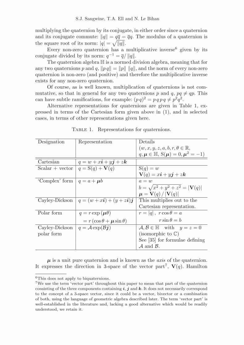
Alternative representations for quaternions are given in Table 1, ex-pressed in terms of the Cartesian form given above in (1), and in selectedcases, in terms of other representations given here.
Table 1. Representations for quaternions.
Designation Representation Details(w, x, y, z, a, b, r, θ ∈ R,q,μ ∈ H, S(μ) = 0,μ2 = −1)
Cartesian q = w + xi + yj + zkScalar + vector q = S(q) + V(q) S(q) = w
V(q) = xi + yj + zk‘Complex’ form q = a + μb a = w
b =√
x2 + y2 + z2 = |V(q)|μ = V(q) / |V(q)|
Cayley-Dickson q = (w + xi) + (y + zi)j This multiplies out to theCartesian representation.
Polar form q = r exp (μθ)
= r (cos θ + μ sin θ)
r = |q| , r cos θ = a
r sin θ = b
Cayley-Dickson q = A exp(Bj) A,B ∈ H with y = z = 0polar form (isomorphic to C)
See [35] for formulae definingA and B.
μ is a unit pure quaternion and is known as the axis of the quaternion.It expresses the direction in 3-space of the vector part7, V(q). Hamilton
6This does not apply to biquaternions.7We use the term ‘vector part’ throughout this paper to mean that part of the quaternion
consisting of the three components containing i, j and k. It does not necessarily correspond
to the concept of a 3-space vector, since it could be a vector, bivector or a combinationof both, using the language of geometric algebra described later. The term ‘vector part’ is
well-established in the literature and, lacking a good alternative which would be readilyunderstood, we retain it.
Fundamental Representations of Biquaternions
himself showed that any unit pure quaternion is a square root of −1 [21,pp 203, 209][17, § 167, p179] and a proof is also given in [9, Lemma 1]. Thisis why we call the form a + μb the ‘complex’ form, since it is isomorphicto a complex number a + Ib. This means that the modulus and argumentof the quaternion are identical to those of a + Ib (one could think of themas having similar Argand diagrams, where in the case of quaternions, theArgand diagram represents a plane section of 4-space defined by the ‘axis’ μand the scalar quaternion axis – along which w is measured).
The polar form of a quaternion is analogous to the polar form of acomplex number, with one exception. The argument, θ, is confined to theinterval [0, π) because the modulus of the vector part is conventionally takento be positive (there is no universally applicable8 coordinate-invariant wayto define an orientation in 3-space which would permit the sign of the vectorpart to be determined). If we negate the argument of the exponential in thepolar form, therefore, the negation is conventionally applied to the axis, μand not to the argument θ. When θ is computed numerically, the result isalways in [0, π) because we have to use the (non-negative) modulus of thevector part to compute it (using an atan2 function, typically).
The Cayley-Dickson polar form [35] has a complex modulus A, and acomplex argument B, (both in fact are degenerate quaternions of the formw + ix, isomorphic to complex numbers).
3. Biquaternions
To generalize the quaternions to biquaternions we simply permit the fourelements to be complex rather than real, thus giving us the Cartesian repre-sentation:
q = W + Xi + Y j + Zk (4)
where i, j and k are exactly as in § 2 and W , X, Y , Z, are complex. Thisgeneralization was first studied by Hamilton himself [19] and [17, § 669, p664],and was also discussed by Cayley [41].
In (4) each of the four elements is of the form W = (W ) + I(W ),where I2 = −1 is the usual complex operator, distinct from i. Axiomatically,I commutes with the three quaternion operators i, j and k, that is iI =Ii, jI = Ij and kI = Ik. Since reals commute with the three quaternionoperators, so do all complex numbers of the form a + Ib, where a, b ∈ R.It is important to maintain a clear conceptual separation between complexnumbers a+ Ib and quaternions of the form a+ bi or a+ bj, which, althoughisomorphic to a complex number, remain quaternions (or biquaternions if thecoefficients are complex). Similarly the ‘complex form’ of a quaternion a+μbin Table 1 is a quaternion, and not a complex number in the sense we aretalking about here since μ is a unit pure quaternion.
8Of course, in specific applications it may be possible to define a reference direction.
S.J. Sangwine, T.A. Ell and N. Le Bihan
Some familiar rules of algebra apply to biquaternions. Since the realand imaginary parts are quite separate from the concept of the four quater-nion components, real and imaginary parts may be equated just as whenworking with complex equations. However, some of the elementary proper-ties of quaternions can become non-elementary when the quaternions arecomplexified. For example, some generalizations of the norm and modulus ofa quaternion are complex in general for biquaternions, and so is the argumentin one of the polar forms. We discuss each of these non-trivial properties ina later section.
The existence of complex generalizations of the norm, modulus and innerproduct, yields a problem of terminology, since conventionally these quanti-ties are real, and satisfy properties that their complex generalizations cannot(the triangle inequality ‖p + q‖ ≤ ‖p‖ + ‖q‖, for example, requires ordering,but complex numbers lack ordering, hence the triangle inequality cannot beapplicable to a ‘norm’ with a complex value). Rather than invent new terms,we use the existing accepted terms (with the exception of norm, where wesubstitute semi-norm, for reasons discussed in § 3.3), but caution the readerthat because these quantities are complex, they cannot be assumed to satisfyall the usual properties of their conventional real equivalents. In taking thisapproach, we are following Synge [40, p 9], and to some extent Ward [42],both of whom use the term norm to refer to a complex generalization. Syngealso refers to a scalar product with a complex value, and Ward uses the terminner product for a complex generalization of the concept in his section onthe Minkowski metric [42, § 3.3, p 115].
Although a biquaternion commutes with its quaternion conjugate, andcomplex numbers commute (including with their complex conjugates), some-what surprisingly, a biquaternion does not necessarily commute with its com-plex conjugate (Proposition 1 in § 3.1).
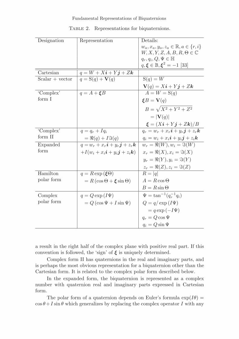
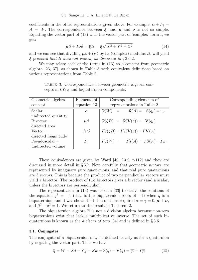
Alternative representations for biquaternions are shown in Table 2, ex-pressed in terms of the Cartesian form given above in (4), and in selectedcases, in terms of other representations given here. In the scalar/vector form,the scalar part is complex, and the vector part is a pure biquaternion.
Complex form I corresponds to the ‘complex’ form in Table 1. Thedifferences are that A and B are now complex, whereas a and b were real,and the imaginary unit ξ is a pure biquaternion root of −1 of the formξ = bμ+dIν, where b2−d2 = 1 and μ and ν are mutually perpendicular unitpure quaternions (themselves also roots of −1) [33]. Note that B can vanish– as discussed in § 3.6.2 and in detail in [34, § 2] – although its components(X, Y and Z), and therefore q, do not vanish. ξ can be thought of as acomplex axis, in the sense that it has real and imaginary parts which eachdefine directions in 3-space. The geometric interpretation of biquaternionsis discussed further in § 3.7. As in the quaternion case, B (the result of thesquare root operation) may be arbitrarily negated, provided ξ is negated tocompensate. Conventionally, the computation of a complex square root yields
Fundamental Representations of Biquaternions
Table 2. Representations for biquaternions.
Designation Representation Details:wa, xa, ya, za ∈ R, a ∈ r, iW,X, Y, Z,A,B,R,Θ ∈ Cqr, qi, Q,Ψ ∈ Hq, ξ ∈ B, ξ2 = −1 [33]
Cartesian q = W + Xi + Y j + ZkScalar + vector q = S(q) + V(q) S(q) = W
V(q) = Xi + Y j + Zk
‘Complex’form I
q = A + ξB A = W = S(q)
ξB = V(q)
B =√X2 + Y 2 + Z2
= |V(q)|ξ = (Xi + Y j + Zk)/B
‘Complex’form II
q = qr + Iqi
= (q) + I(q)
qr = wr + xri + yrj + zrk
qi = wi + xii + yij + zik
Expandedform
q =wr + xri + yrj + zrk
+I(wi + xii + yij + zik)
wr = (W ), wi = (W )
xr = (X), xi = (X)
yr = (Y ), yi = (Y )
zr = (Z), zi = (Z)
Hamiltonpolar form
q = R exp (ξΘ)
= R (cos Θ + ξ sin Θ)
R = |q|A = R cos Θ
B = R sin Θ
Complexpolar form
q = Q exp (IΨ)
= Q (cos Ψ + I sin Ψ)
Ψ = tan−1(q−1r qi)
Q = q/ exp (IΨ)
= q exp (−IΨ)
qr = Q cos Ψ
qi = Q sin Ψ
a result in the right half of the complex plane with positive real part. If thisconvention is followed, the ‘sign’ of ξ is uniquely determined.
Complex form II has quaternions in the real and imaginary parts, andis perhaps the most obvious representation for a biquaternion other than theCartesian form. It is related to the complex polar form described below.
In the expanded form, the biquaternion is represented as a complexnumber with quaternion real and imaginary parts expressed in Cartesianform.
The polar form of a quaternion depends on Euler’s formula exp(Iθ) =cos θ+I sin θ which generalizes by replacing the complex operator I with any
S.J. Sangwine, T.A. Ell and N. Le Bihan
root of −1. In the case of quaternions, the set of unit pure quaternions pro-vides an infinite number of roots of −1 and the general polar form r exp(μθ),as given in Table 1 is therefore a straightforward extension of Euler’s formula.In the case of biquaternions there are two possibilities for the root of −1: thecomplex root I, or any one of the biquaternion roots of −1 defined in § 3.5.Thus we have two possible fundamental polar forms.
The first (‘Hamilton’) polar form generalizes the polar form in the realcase. R, the ‘modulus’ of the biquaternion, is complex; ξ is a biquaternionroot of −1; and Θ, the ‘angle’ in the exponential, is also complex9. Theinterpretation of complex angles is discussed further in § 3.2.
In the second (‘complex’) polar form, the standard complex operator Iserves as the root of −1 in the exponential, but in this form, the ‘argument’ ofthe exponential, Ψ, is a quaternion, and the exponential is scaled by a quater-nion ‘modulus’ Q. We thus have a polar form with a ‘modulus’ and ‘argument’in H. Note that it is not possible to find Q by the obvious direct route ofQ =
√q2r + q2i because qr = Q cos Ψ and squaring this gives Q cos Ψ Q cos Ψ
and not Q2 cos2 Ψ. However, it is the case that cos2 Ψ + sin2 Ψ = 1, as wouldbe expected. Further, note that care is needed in computing the inverse tan-gent in order to find Ψ: it is important that the real part is divided on theleft. This is because
tan Ψ = (Q cos Ψ)−1(Q sin Ψ) = cos−1Ψ Q−1Q sin Ψ = cos−1Ψ sin Ψ (5)
whereas with a division on the right we have:
tan Ψ = (Q sin Ψ)(Q cos Ψ)−1 = Q sin Ψ cos−1Ψ Q−1 (6)
and Q and its inverse are at opposite ends of the product and do not cancel,in general10. (Note that cos Ψ and sin Ψ commute, so their quotient is thesame whether divided on the left or right.) The exponential is a biquaternionbecause of the presence of I and it has a complex modulus. The modulus ofthis complex modulus is 1. We discuss both polar forms further in § 3.1 in thecontext of conjugation. Finally, note that in the complex polar form, Q andthe exponential do not commute. It is therefore possible to define a variantby placing Q on the right of the exponential. The variant is related to theform in Table 2 by the conjugate rule.
De Leo and Rodrigues [8] discussed polar forms of biquaternions butapparently did not see that there were two simple polar forms as here, withdifferent imaginary units. Instead they described a single polar form contain-ing the product of two exponentials. We can do this with either of our polar
9The cosine and sine of a complex angle are simply defined in terms of Euler’s formula
as cos z = 12
(eIz + e−Iz
)and sin z = − 1
2I(eIz − e−Iz
); or, if we write z = x + Iy:
cos z = cosx cosh y− I sinx sinh y and sin z = sinx cosh y+ I cosx sinh y [5, See complexes].10It is of course possible for Q and Ψ to commute in special cases. When this is the case itdoes not matter whether the inverse tangent is computed by dividing the real part on the
left or right, since the result will be the same. Since the left division will give the correctresult in all cases, this is the one that should be implemented numerically.
Fundamental Representations of Biquaternions
forms, representing the ‘modulus’ in each case in its own polar form. Thusthe ‘Hamilton’ polar form can be written:
q = R exp (ξΘ) = r exp (Iφ) exp (ξΘ) (7)
where r, φ ∈ R are the modulus and argument of R, the complex ‘modulus’of q. Note that, because I and ξ commute, the two exponentials commute,and it is possible to write this polar form as:
q = r exp(Iφ + ξΘ) (8)
where the argument of the exponential is now a biquaternion with Iφ asscalar part and ξΘ as vector part. (In general, with quaternions as well asbiquaternions, ep eq = epq because of non-commutativity.)
Similarly, the ‘complex’ polar form can also be written in this way,expanding the quaternion ‘modulus’, Q, into the standard polar form of aquaternion as given in Table 1:
q = Q exp (IΨ) = r exp (μθ) exp (IΨ) (9)
where μ ∈ H and r, θ ∈ R. Notice that the single real modulus r is thesame in each case, but the various ‘angles’ are different in value and type(φ, θ ∈ R,Θ ∈ C,Ψ ∈ H). The real modulus, r, is the absolute value of thesquare root of the semi-norm as discussed in § 3.3. In this case, the argumentsof the two exponentials (specifically μ and Ψ) do not commute in general,hence the two exponentials cannot be combined by adding μθ to IΨ, and nei-ther can the order of the exponentials be changed. In the special case whenμΨ = Ψμ, the vector part of Ψ must be a (real or complex) scalar multipleof μ (commuting quaternions must have the same axis). Combining the ex-ponentials and separating Ψ into scalar and vector parts, we may thereforewrite the quaternion as:
q = r exp (μθ + I (S(Ψ) + V(Ψ))) (10)
= r exp(I S(Ψ)) exp (μθ + IV(Ψ)) (11)
and writing V(Ψ) as αμ, α ∈ C:
= r exp(I S(Ψ)) exp (μ (θ + Iα)) (12)
we find that the axis of the quaternion q is the real unit quaternion μ whichis the axis of Q (the quaternion ‘modulus’ in the polar form). The complexsemi-norm of the quaternion is clearly r exp (I S(Ψ)), and the complex angleis θ + Iα.
We can usefully combine the ‘complex’ representation of a quaternionfrom Table 1 with ‘complex’ form II from Table 2 to give the following rep-resentation, which was used in [33] to derive the biquaternion roots of −1:
q = (α + μβ) + I(γ + νδ) (13)
in which μ and ν are real pure unit quaternions, and α, β, γ and δ arereal. The four real coefficients in this representation may be related to the
S.J. Sangwine, T.A. Ell and N. Le Bihan
coefficients in the other representations given above. For example: α + Iγ =A = W . The correspondence between ξ, and μ and ν is not so simple.Equating the vector part of (13) with the vector part of ‘complex’ form I, weget:
μβ + Iνδ = ξB = ξ√X2 + Y 2 + Z2 (14)
and we can see that dividing μβ+Iνδ by its (complex) modulus B, will yieldξ provided that B does not vanish, as discussed in § 3.6.2.
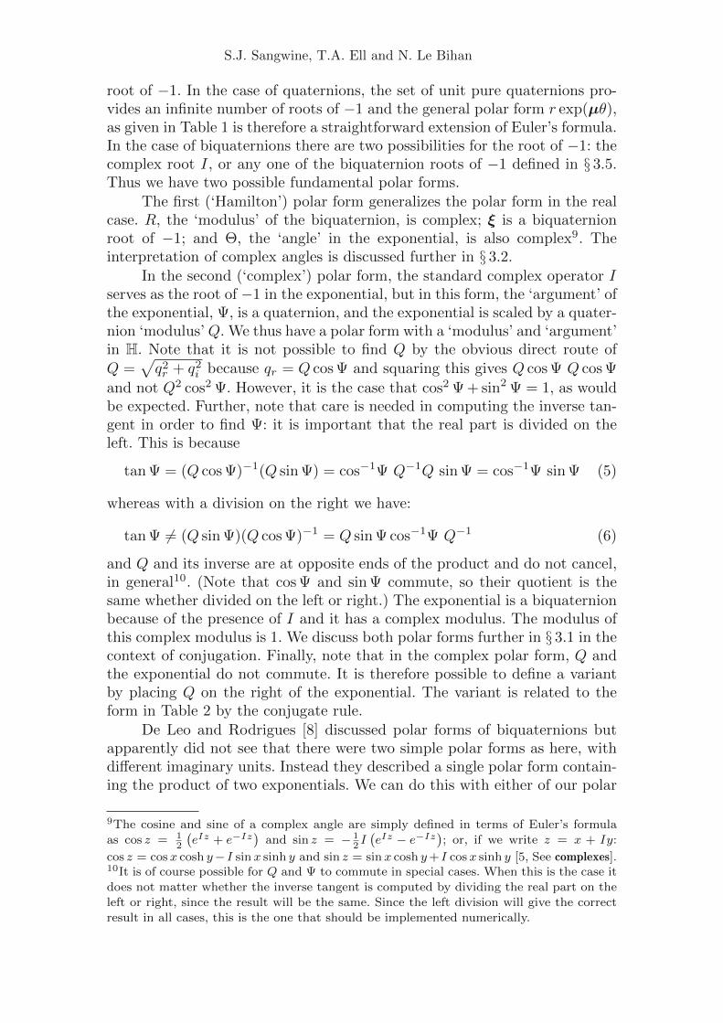
We may relate each of the terms in (13) to a concept from geometricalgebra [23, 37], as shown in Table 3 with equivalent definitions based onvarious representations from Table 2.
Table 3. Correspondence between geometric algebra con-cepts in C3,0 and biquaternion components.
Geometric algebra Elements of Corresponding elements ofconcept equation 13 representations in Table 2
Scalar –undirected quantity
α (W ) = (A) = S(qr) =wr
Bivector –directed area
μβ (ξB) = (V(q)) = V(qr)
Vector –directed magnitude
Iνδ I(ξB) = I(V(q)) = IV(qi)
Pseudoscalar –undirected volume
Iγ I(W ) = I(A) = I S(qi) = Iwi
These equivalences are given by Ward [42, § 3.2, p 112] and they arediscussed in more detail in § 3.7. Note carefully that geometric vectors arerepresented by imaginary pure quaternions, and that real pure quaternionsare bivectors. This is because the product of two perpendicular vectors mustyield a bivector. The product of two bivectors gives a bivector (and a scalar,unless the bivectors are perpendicular).
The representation in (13) was used in [33] to derive the solutions ofthe equation q2 = −1 (that is the biquaternion roots of −1) when q is abiquaternion, and it was shown that the solutions required α = γ = 0, μ ⊥ ν,and β2 − δ2 = 1. We return to this result in Theorem 2.
The biquaternion algebra B is not a division algebra because non-zerobiquaternions exist that lack a multiplicative inverse. The set of such bi-quaternions is known as the divisors of zero [34] and is defined in § 3.6.
3.1. Conjugates
The conjugate of a biquaternion may be defined exactly as for a quaternionby negating the vector part. Thus we have
q = W −Xi− Y j − Zk = S(q) −V(q) = qr + Iqi (15)
Fundamental Representations of Biquaternions
We call this the ‘Hamiltonian’ or quaternion conjugate, in agreement withSynge [40, Equation 3.4, p 8]. The conjugate rule q p = p q and its generaliza-tion to more than two quaternions applies equally to biquaternions. Similarly,a biquaternion commutes with its quaternion conjugate, and the product ofthe two is the semi-norm, as discussed in § 3.3.
However, there is another possible conjugate – that obtained by takingthe complex conjugate of the complex components of the quaternion. Wedenote this complex conjugate by a superscript star, which is a commonconvention with complex numbers. Thus the complex conjugate is given by:
q = W + Xi + Y j + Zk = S(q)
+ V(q)
= qr − Iqi (16)
Our definition in equation 16 agrees with that of Synge [40, p8, equation 3.4]and appears to be the obvious way to define the complex conjugate, but itdiffers from that of Ward [42] who defines a complex conjugate which is aquaternion conjugate with complex conjugate components. There is no wayto define the complex conjugate in terms of additions and multiplications ascan be done with the quaternion conjugate — if a means existed, it wouldalso apply to complex numbers because a degenerate biquaternion of the formα+Iγ with α, γ ∈ R, is isomorphic to a complex number. Instead the complexconjugate must be seen as a fundamental operation. Note very carefully thata biquaternion does not commute with its complex conjugate, a surprisingresult that we examine in Proposition 1 below.
Of course, we can apply both conjugates [42] (we call this a total con-jugate, but the term biconjugate has also been suggested in [12], and weconsider it apposite). It is not difficult to show the following results:
q = q (17)
(pq) = pq (18)
(pq) = q p (19)
In terms of the various representations above, the total or biconjugate is:
q = wr − xri− yrj − zrk − I(wi − xii− yij − zik)
= qr − I qi (20)
= S(q) −V(q)
However, the ramifications of non-commutativity are deep, as shown by thefollowing Proposition.
Proposition 1. A biquaternion does not, in general, commute with its complexconjugate: reversing the order of the product yields a complex conjugate result.
Proof. Represent an arbitrary biquaternion in complex form I, as given inTable 2: q = qr + Iqi. Then the two products of q with its complex conjugateq are:
The results are a complex conjugate pair, and therefore differ. Note that important exceptions to Proposition 1 are:
• Quaternions, that is biquaternions with qi = 0 (trivial).• Imaginary biquaternions, with qr = 0. In this case the product is q2i ,
regardless of order.• Biquaternions with real and imaginary parts that commute (co-planar,
with a common axis). In this case the imaginary part of the productvanishes and the result is q2r + q2i , regardless of order.
The Hamilton and complex conjugates correspond to negation of theargument of the exponential in the two polar forms in Table 2. In the ‘Hamil-ton’ polar form, negating the argument of the exponential negates the sineterm, which corresponds to the vector part of q, and thus yields the classicalHamilton conjugate. In the ‘complex’ polar form, negating the argument ofthe exponential again negates the sine term, but in this case the sine termcorresponds to the imaginary part of the quaternion, and thus it is the com-plex conjugate that is obtained. A third possibility would be a polar formthat would correspond (in the sense just outlined) to the total conjugate.However, this would require the sine term to represent all the components in(20) except wr, which would be represented in the cosine term. This appearsimprobable.
The three types of conjugate allow us to construct formulae for extract-ing the geometric components of a biquaternion, as defined in Table 3. Theformulae in Table 4 are obtained by substitution from four formulae for thescalar/vector and real/imaginary parts of a quaternion based on sums anddifferences of the Hamilton or complex conjugates. Unlike the formulae inequation 3 however, which are based on involutions, and therefore requiremultiplication and addition only, these formulae contain complex conjugates,which are primitive operations that cannot be expressed in terms of mul-tiplications and additions. Similarly, and fairly trivially, by combining theformulae in equation 3 with formulae based on sums and differences of com-plex conjugates, one can obtain formulae for extracting any of the eight realcomponents of a biquaternion11. For example, that for the real part of thescalar part is wr = 1
8 (q+q−iqi−iqi−jqj−jqj−kqk−kqk). Finally wenote that the operations represented by the formulae in Table 4 are known ingeometric algebra as ungrading operations which return the different ‘grades’within a multivector [30, § 6.1.3].
3.2. Inner Product
The definition of the inner product in the classic quaternion case was given byPorteous [32, Prop. 10.8, p 177] and we take this as the basis for defining theinner product of two biquaternions, since it is consistent with the quaternioncase, and also yields the semi-norm (see the next section) in the case of the
11The utility of such formulae is not in numeric computation, where explicit access to the
components is a much better approach, but in algebraic manipulation, where the formulaemay allow an algebraic solution to an otherwise seemingly difficult derivation.
Fundamental Representations of Biquaternions
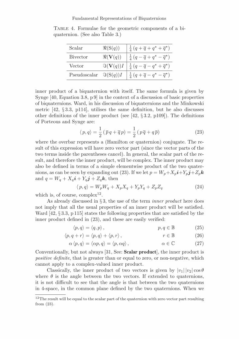
Table 4. Formulae for the geometric components of a bi-quaternion. (See also Table 3.)
Scalar (S(q)) 14 (q + q + q + q)
Bivector (V(q)) 14 (q − q + q − q)
Vector (V(q))I 14 (q − q − q + q)
Pseudoscalar (S(q))I 14 (q + q − q − q)
inner product of a biquaternion with itself. The same formula is given bySynge [40, Equation 3.8, p 9] in the context of a discussion of basic propertiesof biquaternions. Ward, in his discussion of biquaternions and the Minkowskimetric [42, § 3.3, p114], utilises the same definition, but he also discussesother definitions of the inner product (see [42, § 3.2, p109]). The definitionsof Porteous and Synge are:
〈 p, q〉 =1
2( p q + q p) =
1
2( p q + q p) (23)
where the overbar represents a (Hamilton or quaternion) conjugate. The re-sult of this expression will have zero vector part (since the vector parts of thetwo terms inside the parentheses cancel). In general, the scalar part of the re-sult, and therefore the inner product, will be complex. The inner product mayalso be defined in terms of a simple elementwise product of the two quater-nions, as can be seen by expanding out (23). If we let p = Wp+Xpi+Ypj+Zpkand q = Wq + Xqi + Yqj + Zqk, then
〈 p, q〉 = WpWq + XpXq + YpYq + ZpZq (24)
which is, of course, complex12.As already discussed in § 3, the use of the term inner product here does
not imply that all the usual properties of an inner product will be satisfied.Ward [42, § 3.3, p 115] states the following properties that are satisfied by theinner product defined in (23), and these are easily verified:
〈p, q〉 = 〈q, p〉 , p, q ∈ B (25)
〈p, q + r〉 = 〈p, q〉 + 〈p, r〉 , r ∈ B (26)
α 〈p, q〉 = 〈αp, q〉 = 〈p, αq〉 , α ∈ C (27)
Conventionally, but not always [31, See: Scalar product], the inner product ispositive definite, that is greater than or equal to zero, or non-negative, whichcannot apply to a complex-valued inner product.
Classically, the inner product of two vectors is given by |v1| |v2| cos θwhere θ is the angle between the two vectors. If extended to quaternions,it is not difficult to see that the angle is that between the two quaternionsin 4-space, in the common plane defined by the two quaternions. When we
12The result will be equal to the scalar part of the quaternion with zero vector part resultingfrom (23).
S.J. Sangwine, T.A. Ell and N. Le Bihan
extend this concept to biquaternions, the angle between them, and theirmoduli, must be complex, in general, so the geometric interpretation of theinner product is slightly more difficult. In the quaternion case, orthogonalityarises from the angle between the two quaternions (having a vanishing cosine),but in the biquaternion case there is the additional possibility that one orboth moduli are zero, resulting in a vanishing inner product. Expressing theinner product of two biquaternions in terms of inner products of the realand imaginary parts makes it possible to understand what the inner productrepresents geometrically. Representing p as follows: p = pr+Ipi and similarlyfor q, the inner product may be expanded as:
Certain special cases are apparent after careful inspection:
• 〈p, q〉 = 0 indicates that the two biquaternions are orthogonal or ‘per-pendicular’, and it requires the real and imaginary parts of the innerproduct to vanish separately. The detailed conditions required for thisare many, since the four inner product components (two real, two imagi-nary) may have positive or negative real values and can cancel in severalways. We list here four different ways in which the scalar product canvanish:
Strongest constraint. This is when all four real and imaginary partsof the two biquaternions are mutually orthogonal. A simple ex-ample is p = 1 + Ii and q = j + Ik, but it is easy to con-struct a more general example starting from a random quaternion.Let p1 be a randomly chosen (pure or full) quaternion. Then letp2 = p1i, p3 = p1j and p4 = p1k
13. The four quaternions thus con-structed have the same four numeric components permuted withsign changes in such a way that any two will have a vanishing innerproduct14. Two biquaternions p = p1 + Ip2 and q = p3 + Ip4 (orany other permutation) will have 〈p, q〉 = 0. This pair of biquater-nions will be found to be divisors of zero (see § 3.6), but scaling thereal and imaginary parts with different scale factors will result inbiquaternions that are not divisors of zero, but are still orthogonal(orthogonality not being dependent on norm). Choosing the initialrandom value to be pure does not result in the pair of biquaternionsbeing pure, because of permutation of the components.
Weaker constraint I.1. The real parts of the two biquaternions are orthogonal, and
the imaginary parts of the two biquaternions are orthogonal,hence the real part of the scalar product vanishes because itis the difference of two vanishing scalar products.
13Any set of three mutually orthogonal unit pure quaternions may be used here in place
of i, j and k, and similarly in the next two cases.14Three other permutations can be obtained by multiplication on the right, or by divisionon either side by i, j and k.
Fundamental Representations of Biquaternions
2. The real part of each biquaternion is not orthogonal to theimaginary part of the other. However, the scalar products ofthe real part of one biquaternion with the imaginary partof the other have the same values, but opposite signs. Thismeans the imaginary part of the scalar product of the twobiquaternions vanishes by cancellation.
A pair of biquaternions satisfying this constraint can be obtainedfrom an arbitrary biquaternion p, by choosing q = p i (and twoothers also orthogonal to the first may be constructed by choosingq = pj or q = pk)15.
Weaker constraint II.1. The real parts of the two biquaternions are not orthogonal,
and neither are the imaginary parts, but the scalar productof the two real parts has the same value and sign as the scalarproduct of the two imaginary parts. This means the real partof the scalar product of the two biquaternions vanishes bycancellation.
2. The real part of each biquaternion is orthogonal to the imagi-nary part of the other, hence the imaginary part of the scalarproduct of the two biquaternions vanishes because it is thesum of two vanishing scalar products.
A pair of biquaternions satisfying this constraint can be obtainedfrom an arbitrary biquaternion p, by choosing q = p Ii (and ditto,mutatis mutandis.).
Weakest constraint. This is when none of the real and imaginaryparts of the two biquaternions are orthogonal, but the real andimaginary parts of the scalar product of the two biquaternionsvanish by cancellation. A pair of biquaternions satisfying this con-straint can be constructed from an arbitrary biquaternion p, bychoosing q = p(i+ Ij) or similar. Note that this results in q beinga divisor of zero (see § 3.6) because (i + Ij) is a divisor of zero.
• 〈p, q〉 is real, that is with zero imaginary part. There is a trivial case:the two biquaternions may be imaginary with zero real parts. Other-wise, the imaginary part of the inner product can vanish in two ways,as in the weaker cases above of 〈p, q〉 = 0: either the imaginary partvanishes by cancellation, or it vanishes because the real part of each bi-quaternion is orthogonal to the imaginary part of the other. It is easy toconstruct a biquaternion to satisfy the second condition using the tech-nique outlined above for the strongest constraint: construct two pairsof orthogonal quaternions, and then construct two biquaternions usingthe components of these pairs.
• 〈p, q〉 is imaginary, that is with zero real part. The conditions requiredfor this are very similar to the previous case, with the appropriate
15As in the stronger case, it is also possible to multiply by i on the left, etc.
S.J. Sangwine, T.A. Ell and N. Le Bihan
changes. A trivial case is where one biquaternion is real and the otheris imaginary.
Clearly, from the above analysis, orthogonality of biquaternions is not as sim-ple as orthogonality of real quaternions where a geometrical interpretation interms of a plane and a real angle is straightforward. In the biquaternion case,interpreting the inner product 〈p, q〉 as |p| |q| cos Θ, where the two moduli andthe angle are complex, is not at all obvious. This remains a topic for furtherwork.
3.3. Semi-norm
In this section we consider the generalization of the quaternion norm ‖q‖ =w2 + x2 + y2 + z2, ‖q‖ ∈ R to the biquaternion case by allowing the fourCartesian components to become complex. Conventionally a norm is real andpositive definite, that is non-negative, but in the case of biquaternions, thisconvention must be relaxed because the norm has a complex value. Addi-tionally, the existence of divisors of zero (see § 3.6) means that a non-zerobiquaternion can have a vanishing norm. For this reason, we use the termsemi-norm. A semi-norm is a generalization of the concept of a norm, withno requirement that the norm be zero only at the origin (of a vector space)[4, See: semi-norm]. As with our use of the term inner product in § 3.2 fora complex-valued generalization of the inner product, we are here extendingthe term semi-norm to a complex-valued quantity analogous to a norm, withthe additional property of vanishing in the case of divisors of zero. We alsouse the term modulus for the square root of the semi-norm – and since thesemi-norm is complex, we define the modulus to be complex, in general (insome cases it may be real).
The semi-norm can be real and negative in special cases, as well as purelyimaginary. The semi-norm can be defined in terms of the inner product ofa biquaternion with itself, that is ‖q‖ = 〈q, q〉 or directly in terms of the
four complex components: ‖q‖ = |q|2 = W 2 + X2 + Y 2 + Z2. Although thesemi-norm is complex-valued the result given by Coxeter for quaternions [7,
§ 2] still holds: ‖q‖ = |q|2 = q q = q q. This is, of course, a special case of theformula for the inner product, in this case of q with itself (23).
Lemma 1. [34, Lemma 1] Let q = qr + Iqi be a non-zero biquaternion withreal part qr ∈ H and imaginary part qi ∈ H. The real part of ‖q‖ is equal tothe difference between the norms of qr and qi, and the imaginary part of ‖q‖is equal to twice the inner product of qr and qi:
‖q‖ = ‖qr‖ − ‖qi‖ + 2I 〈qr, qi〉 (29)
Proof. We express the semi-norm of q as the product of q with its quaternionconjugate: ‖q‖ = qq. Writing this explicitly:
The real part of ‖q‖ can be recognised as ‖qr‖ − ‖qi‖ from Coxeter’s result[7, § 2]. The imaginary part of ‖q‖ is twice the inner product of qr and qi asgiven by Porteous [32, Prop. 10.8, p 177] and (23).
There are some special cases of the result given in Lemma 1:
• biquaternions with perpendicular real and imaginary parts have a realsemi-norm (because the imaginary part vanishes), but the semi-normmay be negative if the norm of the imaginary part exceeds the norm ofthe real part;
• biquaternions with real and imaginary parts with equal norms have animaginary semi-norm (because the real part vanishes).
• imaginary biquaternions (with qr = 0) have a negative real semi-norm,and therefore an imaginary modulus.
• biquaternions with perpendicular real and imaginary parts with equalnorms have a vanishing semi-norm. This important special case is cov-ered in more detail in § 3.6.
The semi-norm is invariant under quaternion conjugation, that is ‖q‖ =‖q‖, but under complex conjugation the semi-norm of the conjugate equalsthe complex conjugate of the semi-norm: ‖p‖ = ‖p‖. This can be seen easilyfrom Lemma 1, since quaternion conjugation does not affect the norms of thereal and imaginary parts, nor their inner product. However, although complexconjugation does not alter the norms of the real and imaginary parts, it doesnegate their inner product and therefore negates the imaginary part of thesemi-norm.
The semi-norm as defined here (and by Ward [42, § 3.3, p 115]) obeysthe ‘rule of the norms’16 so that for any two biquaternions, the semi-normof their product equals the product of their semi-norms: ‖p q‖ = ‖p‖ ‖q‖.This is true even in the case where one or both of p and q is a divisor ofzero, with vanishing semi-norm, as discussed in § 3.6 (but the result will bezero, computed as the semi-norm of the product, or the product of the semi-norms). Hence B is a normed algebra using the definition of the semi-normused in this section. The non-zero biquaternions that have zero semi-norm(the divisors of zero) lack a multiplicative inverse.
We now consider the properties of the modulus, or square root of thesemi-norm as defined above. What we here call the modulus is usually re-quired to satisfy the following three properties [4, See: norm]17. In fact only
16The ‘rule of the norms’ holds also for the modulus (the square root of the semi-norm),
which is what the term ‘norm’ refers to in many sources in the literature.17The cited reference states these properties using the notation ‖x‖ where we use |x| andit uses the term ‘norm’ to mean what is here called ‘modulus’.
S.J. Sangwine, T.A. Ell and N. Le Bihan
the second of these is valid for biquaternions.
|λx| = |λ| |x| (Not valid for x ∈ B) (32)
|−x| = |x| (33)
|x + y| ≤ |x| + |y| (Triangle inequality – not applicable for x ∈ B) (34)
The first of these properties does not hold for biquaternions because λ isusually taken to be a scalar, that is in the biquaternion context, a complexnumber. The formula assumes that |λ| equals λ apart from sign, which isnot true for complex numbers. However, a similar formula for the semi-normdoes apply to biquaternions: ‖λx‖ = λ2 ‖x‖. This can be shown as follows:noting that ‖q‖ = 〈q, q〉 for all q ∈ B and using the third property of the innerproduct given in (27), we have that λ2 〈q, q〉 = 〈λq, λq〉 and hence the result
stated. However, taking the square root of both sides gives |λx| =√λ2 |x|.
The square root of the square of a complex number is neither the modulus ofthe complex number, nor necessarily the original complex number: the resultof the square root is always in the right half-plane (because the argument ishalved by the square root operation). The second of these properties is easilyseen to be satisfied for all q ∈ B because negating a complex number doesnot change its square, and therefore does not alter the sum of the squaresof the four components of a biquaternion, nor the square root of the sum ofthe squares. The triangle inequality, as has already been noted in § 3 is notapplicable to the biquaternion semi-norm, because ordering is not defined forcomplex numbers.
3.4. Real norms
It is possible to define more than one norm for the biquaternions includingsome which are real-valued (see for example [42, §§ 3.2 and 3.3]).
There is only one possible real-valued norm which satisfies the ‘rule ofthe norms’. Gurlebeck and Sprossig [13, Lemma 1.30] state that there is aunique real norm satisfying ‖p q‖ = ‖p‖ ‖q‖ and ‖μσ0‖ = |μ| , μ ∈ R whereσ0 is the 2 × 2 identity (Pauli) matrix. This norm is simply the square rootof the absolute value of the semi-norm, in other words, r in equations 7 and9, or |Q| in Table 2.
There is another way to define a real norm [42, § 3.2, p 109], which doesnot satisfy the ‘rule of the norms’, as we would expect, since this norm differsfrom that given by Gurlebeck and Sprossig:
‖q‖ = S(qq
)= ‖qr‖ + ‖qi‖ (35)
= w2r + x2
r + y2r + z2r + w2i + x2
i + y2i + z2i (36)
If we define a modulus (as the square root of this norm), the modulus satisfiesthe properties in (32), including the triangle inequality. Finally, note that thisnorm can be seen as a special case of the following real-valued inner product:〈p, q〉 = 〈pr, qr〉 + 〈pi, qi〉. This is easily seen from (36).
Fundamental Representations of Biquaternions
3.5. Roots of −1
This section draws on and builds on results first presented by Sangwine in[33]. These results have been generalized to Clifford algebras by Hitzer andAblamovicz [25] where the concept is aptly referred to as geometric roots of−1.
Biquaternion roots of -1 appear as ξ in Table 2, in the ‘complex’ and‘Hamilton polar’ forms.
Theorem 1. Any non-zero quaternion or biquaternion with a non-vanishingmodulus, divided by its modulus has a unit real norm.
Proof. Let q be an arbitrary quaternion or biquaternion and let p = q/ |q|.For any quaternion or biquaternion x we have ‖x‖ = xx and |x| =
√‖x‖.
Therefore p = q/√qq and we can write the norm of p as:
‖p‖ = p p =q√q q
(q√q q
)(37)
Since√q q is complex, it is unaffected by the quaternion conjugate and we
can simplify this to:
=q√q q
q√q q
=q q
q q= 1 (38)
Theorem 2. Any pure quaternion or biquaternion with a non-vanishing mod-ulus, divided by its modulus, is a root of −1.
Proof. Let q be an arbitrary quaternion or biquaternion with |q| = 0. Then
(q/ |q|)2 = q2/q q = q/q. If we restrict q to have zero scalar part, the conjugate
reduces to negation and we have (q/ |q|)2 = q/− q = −1.
Theorem 2 is simply a restatement of the well-known fact that unit purequaternions are roots of −1 [17, § 167, p179], but in the case of biquaternions,the ramifications of the result are not so obvious. Theorem 2 is also easilydemonstrated using the Cartesian form:
(Xi + Y j + Zk√X2 + Y 2 + Z2
)2
=
⎛⎜⎝
−X2 + XY (ij + ji)
−Y 2 + XZ(ik + ki)
−Z2 + Y Z(jk + kj)
⎞⎟⎠ /(X2 + Y 2 + Z2)
=−(X2 + Y 2 + Z2
)
X2 + Y 2 + Z2= −1 (39)
It was shown in [33, Theorem 2.1] that any pure biquaternion ξ sat-isfying the constraints (ξ) ⊥ (ξ) and ‖(ξ)‖ − ‖(ξ)‖ = 1 is a root of−1 and that no other biquaternions are roots of −1. It follows therefore thatdividing an arbitrary pure biquaternion by its (complex) modulus producesa result that satisfies the constraints stated. Since these constraints are by nomeans obvious from (39), it is interesting to verify them directly. To verify the
S.J. Sangwine, T.A. Ell and N. Le Bihan
constraints stated, we take an arbitrary pure biquaternion p, divide it by its(complex) modulus and show that the result satisfies the constraints stated.Dividing p by its modulus gives a root of −1: ξ = p/ |p|. We have to show thatthe real and imaginary parts of ξ are orthogonal, that is 〈(ξ),(ξ)〉 = 0,and also that the difference between the norms of the real and imaginaryparts of ξ is 1. We can express the real and imaginary parts of ξ as follows,by taking the sum and difference of ξ with its complex conjugate:
(ξ) =1
2(ξ + ξ), (ξ) =
1
2I(ξ − ξ) (40)
The inner product of two quaternions is given by (23), but since we aredealing with pure quaternions, the conjugates reduce to negation, and theinner product simplifies to:
〈u, v〉 = −1
2(uv + vu) (41)
Substituting the results above for the real and imaginary parts of ξ, we obtainthe following:
〈(ξ),(ξ)〉 = −1
2
[1
2(ξ + ξ)
1
2I(ξ − ξ) +
1
2I(ξ − ξ)
1
2(ξ + ξ)
]
= − 1
8I[(ξ + ξ) (ξ − ξ) + (ξ − ξ) (ξ + ξ)]
= − 1
8I
[ξ2 + ξξ − ξ
2 − ξξ + ξ2 − ξξ − ξ2
+ ξξ]
= − 1
4I
[ξ2 − ξ
2]
(42)
Since ξ is a root of −1 by Theorem 2, its complex conjugate must also be a
root of minus one18, thus ξ2 = ξ2
= −1 and therefore 〈(ξ),(ξ)〉 = 0 asexpected.
To show that the real and imaginary parts of ξ have norms differing by1, we can use a similar approach. Starting with the fact that the norm is theinner product of a quaternion with itself, as stated in § 3.3, the formula in(41) simplifies to ‖u‖ = −u2 when u is pure and v = u. Thus the differencebetween the norms of the real and imaginary parts of ξ is given by:
‖(ξ)‖ − ‖(ξ)‖ = −(ξ)2 + (ξ)2
= −[1
2(ξ + ξ)
]2+
[1
2I(ξ − ξ)
]2
= −1
4
[ξ2 + ξ
2+ ξξ + ξξ
]− 1
4
[ξ2 + ξ
2 − ξξ − ξξ]
= −1
2
[ξ2 + ξ
2]
(43)
which is 1 because ξ and its conjugate are roots of −1.
18This is easily shown using the ‘complex’ form ξ = ξr + Iξi, since the imaginary part
must be zero in both ξ2 and ξ2 if they are each equal to −1.
Fundamental Representations of Biquaternions
3.6. Divisors of zero
It is possible for the semi-norm, ‖q‖, of a biquaternion to be zero, even thoughq = 0. In modern terminology, the biquaternions with vanishing semi-normare better known as divisors of zero. The ‘rule of the norms’ given in § 3.3shows that multiplying an arbitrary biquaternion by a divisor of zero (withvanishing semi-norm) yields a result which is also a divisor of zero (withvanishing semi-norm).
The conditions for the semi-norm to vanish were discovered by Hamilton[17, Lecture VII, § 672, p669]19 — if we represent a non-zero biquaternion inthe form: q = qr + Iqi then its norm is zero iff ‖qr‖ = ‖qi‖ and 〈qr, qi〉 = 0,that is, the real and imaginary parts must have equal norms and be perpen-dicular in 4-space. This result follows easily from (29) in Lemma 1 (§ 3.3).The conditions stated are equivalent to the condition W 2+X2+Y 2+Z2 = 0,which can be expanded into a pair of simultaneous equations each equivalentto one of the two conditions above, by equating the real and imaginary partsto zero separately [34, Proposition 1]. Notice that the conditions required fora vanishing semi-norm may be satisfied in the case of a pure biquaternion(the real and imaginary components are then perpendicular in 3-space). Itfollows from these conditions that any non-zero quaternion or any non-zeroimaginary biquaternion must have a non-zero norm, since the constraint ofreal and imaginary parts having equal norm is violated.
Sangwine and Alfsmann have shown in [34] that every biquaterniondivisor of zero is one of:
• an idempotent as defined in the next section in Theorem 3;• a complex multiple of an idempotent (dividing the divisor of zero by
twice its scalar part yields an idempotent);• a nilpotent as defined in § 3.6.2.
3.6.1. Idempotents. An idempotent is a value that squares to give itself. Anexample of a biquaternion idempotent is given in [12] (quoting a paper ofLanczos from 1929) but no general case is given in the paper. More recentlybiquaternion idempotents were analysed in [1, § 7.1] using a matrix represen-tation of the isomorphic Clifford algebra C3,0.
We present here a derivation of the set of idempotents in B, drawing onresults presented in [34] by Sangwine and Alfsmann.
Theorem 3. [34, Theorem 2] Any biquaternion of the form q = 12± 1
2ξI, whereξ ∈ B is a root of −1, is an idempotent. There are no other idempotents inB.
Proof. The proof is by construction from an arbitrary biquaternion repre-sented in the form q = A + ξB (A,B ∈ C). Squaring and equating to qgives:
q2 = A2 −B2 + 2ABξ = A + ξB = q (44)
19In [17, Lecture VII, § 673, p671], Hamilton rather quaintly refers to an evanescent tensor— a tensor being what we here call a semi-norm.
S.J. Sangwine, T.A. Ell and N. Le Bihan
Equating coefficients of 1 and ξ (that is, equating the real and imaginaryparts with respect to ξ) gives:
A = A2 −B2 (45)
B = 2AB (46)
The second of these equations requires that A = 12 . Making this substitution
into the first equation gives: 12 = 1
4 − B2, from which B2 = − 14 . Since B is
complex, the only solutions are B = ±I/2. Thus q = 12 ± ξI
2 .
The roots of −1 in B include two trivial cases, as noted in [33, Theorem2.1]. These are ±I which yields the trivial idempotents q = 0 and q = 1; and±μ where μ is a real pure quaternion root of −1.
Since every biquaternion idempotent, q, is a solution of q2 = q, it mustalso be a solution of q(q − 1) = 0. Therefore every biquaternion idempotentis also a divisor of zero and must satisfy the conditions stated in § 3.6. Thisis demonstrated in detail in [34, § 4, Proposition 2].
All non-pure biquaternion divisors of zero have been shown to be of theform p = αq where α is a non-zero complex number, and q is a biquaternionidempotent [34, § 4, Theorem 3]. Further, dividing a non-pure biquaterniondivisor of zero by twice its scalar part yields an idempotent [34, § 4, Corollary1].
3.6.2. Nilpotents. A nilpotent is a quantity whose square vanishes. Hamiltondiscovered nilpotent biquaternions and was aware that all such biquaternionswere divisors of zero [17, Lecture VII, § 674, pp671-3].
We first present the case of a pure biquaternion with vanishing semi-norm and show a result due to Hamilton [17, Lecture VII, § 672, p669] thatthe square of such a biquaternion vanishes.
Theorem 4. Let p = pr + Ipi be a non-zero pure biquaternion with vanishingsemi-norm. Then p2 = 0.
Proof. From the fact that p has a vanishing semi-norm, ‖pr‖ = ‖pi‖, thereforewe may divide by their common norm, and obtain p/ ‖pr‖ = μ + Iν whereμ and ν are perpendicular unit pure quaternions. Then:
(p
‖pr‖
)2
= (μ + Iν)2 = μ2 − ν2 + I(μν + νμ) (47)
which vanishes because the squares of the two unit pure quaternions are −1and the imaginary part vanishes because the products of two perpendicularunit pure quaternions changes sign when the order of the product is reversed.
Sangwine and Alfsmann, in [34, § 5, Lemma 1] have shown that all nilpo-tent biquaternions are pure, and in [34, § 5, Proposition 3] that all nilpotentbiquaternions are divisors of zero. It follows that all nilpotent biquaternionshave real and imaginary parts with equal norm and therefore that any nilpo-tent biquaternion can be normalised to the form μ+ Iν as in Theorem 4. We
Fundamental Representations of Biquaternions
see therefore that all nilpotent biquaternions are constructed from a pair ofmutually orthogonal unit pure quaternions.
All nilpotent biquaternions are pure. Non-nilpotent pure biquaternionsmay be expressed in the form q = ξB where ξ is a root of −1 and B iscomplex (the square root of the semi-norm: B =
√X2 + Y 2 + Z2). Since a
nilpotent biquaternion q is a divisor of zero, its semi-norm, and therefore B,is zero, even though q = 0. A consequence is that it is not possible to computethe ‘axis’ ξ of a nilpotent biquaternion q by dividing q by B.
3.7. The biquaternions as a geometric algebra
In this section we discuss equivalences between the biquaternions and geomet-ric algebra [23, 24, 29, 37, 39]. In particular, since there are many geometricalgebras of different dimension, we consider the particular case of the Cliffordalgebra C3,0 to which the biquaternion algebra is isomorphic.
Hamilton himself, in his Lectures on Quaternions [17, Lectures I, II, III]was interested in an algebra of points, lines and planes, and clearly was mo-tivated by a desire to have an algebra applicable to 3-dimensional geometry.The modern notion of a geometric algebra uses different language, and someof the concepts are more sophisticated, but essentially the aim is the same:to represent and manipulate geometric objects algebraically.
The geometric algebra C3,0 (and therefore the biquaternion algebra,through isomorphism) contains four types of element, as already introducedin § 3 and Tables 3 and 4: scalars, vectors, bivectors and pseudoscalars. Scalarsare quantities without geometric form, vectors represent directed magnitudes,bivectors represent directed areas, and pseudoscalars represent signed vol-umes. The product of two perpendicular vectors is a bivector, representingthe area swept out by one vector when moved along the other [39, § 2.1].This is why vectors are identified with pure imaginary biquaternions. Giventwo perpendicular pure quaternions, μ and ν, such that 〈μ,ν〉 = 0, the twovectors Iμ and Iν have a product −μν which is perpendicular to both μand ν. The negative sign is a consequence of squaring I. Changing the orderof the two vectors changes the sign of the resulting bivector (it is oppositelydirected), so the minus sign is of little consequence. It is usual in geometric al-gebra to have to choose the sense of the product of two vectors by conventionand this applies also to the quaternions/biquaternions, where the choice isbetween ijk = −1 (the usual choice) or kji = −1, giving oppositely handedcoordinate systems. The product of three orthogonal vectors defines a vol-ume, represented by a pseudoscalar. For example, (Ii)(Ij)(Ik) = I, as givenby Ward [42, p 113].
There has been much confusion caused by the use of the term vectorwhen in fact the objects under consideration were bivectors. In physics theconcepts of axial and polar vectors have been used, causing further confu-sion, because the two terms suggest different types of vector, rather thanfundamentally different types of quantity. Even the present authors, in theirearlier works, used the term vector to refer to quantities which are now clearly
S.J. Sangwine, T.A. Ell and N. Le Bihan
Table 5. Biquaternion basis multiplication table.
1 iI jI kI i j k I
1 1 iI jI kI i j k IiI iI 1 −k j −I kI −jI −ijI jI k 1 −i −kI −I iI −jkI kI −j i 1 jI −iI −I −ki i −I kI −jI −1 k −j iIj j −kI −I iI −k −1 i jIk k jI −iI −I j −i −1 kII I −i −j −k iI jI kI −1
seen to be bivectors. Unfortunately, the scalar/vector part terminology com-monly applied to quaternions has this wrong, and we are stuck with it: thevector part of a (bi)quaternion is simply that part which is not the scalarpart – it may be a (geometric algebra) vector, a bivector or a combination ofboth20. Similarly, we must be careful not to confuse the scalar part of a bi-quaternion with the geometric algebra concept of a scalar: the scalar part ofa biquaternion is a complex number consisting of the scalar and pseudoscalarparts of the biquaternion.
In the geometric algebra C3,0 a composite quantity consisting of twoor more of the four types of quantity (scalar, vector, bivector, pseudoscalar)is called a multivector. A biquaternion may contain all four types of geo-metric quantity, and except in degenerate cases (such as a pure imaginarybiquaternion), corresponds to the concept of a multivector.
Although multivectors in C3,0 are regarded as composites of scalar,vector, bivector and pseudoscalar, a biquaternion is not constructed in thisway. Instead it has four complex components, but as we have seen in § 3, it ispossible to interpret these in multiple ways, for example as a complex numberwith quaternion components. It is also possible to consider the biquaternionsas 8-dimensional quantities with basis (1, iI, jI,kI, i, j,k, I) where we placethe vector basis first. The multiplication table is then easily derived fromthe rules of quaternion multiplication (Table 5). The table is in 1:1 corre-spondence with the multiplication table for C3,0 — this is the basis of theisomorphism between the two algebras.
From the rules of quaternion multiplication, it is fairly easy to draw upa table showing how the geometric components of a biquaternion multiplytogether. Table 6 shows the result. The four centre entries apply in the generalcase, but in the specific cases where the bivector/vector are perpendicular,the scalar or pseudoscalar part of the product will be zero. Multiplication by
20The same word causes another terminology problem in the field of matrices of quater-nions, where a matrix with one row or column is known as a vector, using the usual matrix
terminology. Of course it is nothing to do with the vector part of a quaternion, or indeedthe vector part of a quaternion matrix.
Fundamental Representations of Biquaternions
Table 6. Multiplication table for components of a biquater-nion multivector
S B V P
S – scalar S B V PB – bivector B S + B P + V VV –vector V P + V S + B BP – pseudoscalar P V B S
Table 7. Correspondence between components of the C3,0algebra and the biquaternions.
the inverse of the pseudoscalar21 is known as the dual operation: it maps abivector into a perpendicular vector, and a scalar into a pseudoscalar or viceversa. The notion of perpendicular depends on an inner product [24, p 10]:
Two multivectors are said to be orthogonal or perpendicular to oneanother, if their inner product is zero.
However, the inner product defined in (23) is not zero for j and −jI which area perpendicular pair of bivector and vector respectively. It is not straight-forward to consider other possible inner products by simply replacing thequaternion conjugation in (23) with a complex or total conjugate, or withno conjugate. We note the following in support of this assertion, and thenleave it for future work: a biquaternion does not commute with its complexconjugate. This means there are several possible variants of (23) if we replacethe quaternion conjugates with complex conjugates, by varying the order ofthe multiplicands in each term.
The biquaternions are isomorphic to the Clifford algebra C3,0 [13,§ 1.1.3 and p 22]. The basis vectors of C3,0 are conventionally written e1,e2 and e3 although sometimes other notations are used22. Table 7 shows thecorrespondences between the basis elements of a biquaternion and a C3,0multivector. Notice that the Clifford basis vectors are multiplied cyclically to
21The inverse of the pseudoscalar in the biquaternion algebra is 1/I, that is −I.22The basis elements in [13] are written as σi, i ∈ 0, 1, 2, 3 otherwise known as the Pauli
matrices.
S.J. Sangwine, T.A. Ell and N. Le Bihan
give the basis bivectors. Thus the biquaternion j is isomorphic to the Cliffordbivector −e3e1 = +e1e3. The quaternions are a subset of the biquaternions,and the corresponding subset in the Clifford algebra C3,0 is known as theeven grade part C+3,0.
3.7.1. Outer products. In geometric algebra, the algebraic or geometric prod-uct of two vectors is the sum of the scalar product and the wedge (∧) or outerproduct:
p q = p · q + p ∧ q (48)
It is possible to define an outer product for quaternions and biquaternionsusing a formula widely used in geometric algebra [39, Equation 3.10]:
1
2(p q − q p) (49)
This formula gives the cross product of the vector parts (because the compo-nents of the products involving the scalar parts, and the dot product of thevector parts, commute and therefore cancel). If applied to a pair of vectors(i.e. pure biquaternions with zero real part), the result is a bivector (i.e. apure biquaternion with zero imaginary part). Applied to a pair of bivectors(pure quaternions) the result is another bivector. Applied to a vector anda bivector, the result is a vector. This indicates that the formula as statedmixes several geometric algebra concepts. As with the various possible for-mulations of the inner product discussed in the previous section, we couldconsider variants of the formula using one or more of the three types of bi-quaternion conjugation, but as with the inner products, we leave this forfurther work.
4. Further Work
There is further interpretation needed of the biquaternions as a geometricalgebra, making use of the isomorphism between biquaternions and C3,0.As discussed in the previous section, the inner and outer product formulaecan be studied, and matched to formulae already known for C3,0 to give anexplicit set of geometric formulae expressed in terms of B.
The interpretation of complex angles in the polar form and in the con-text of the inner product also requires further work.
Acknowledgements
This paper was started in 2005 at the Laboratoire des Images et des Signaux(now part of the GIPSA-Lab), Grenoble, France with financial support fromthe Royal Academy of Engineering of the United Kingdom and the CentreNational de la Recherche Scientifique (CNRS).
Thanks are due to Dr Sebastian Miron, who gave a short series of sem-inars on biquaternions in Grenoble in 2005, and thus started us on the road
Fundamental Representations of Biquaternions
to this paper. We also acknowledge the contribution made by Daniel Alfs-mann who, working with one of us, and using his knowledge of hypercomplexalgebras in general, greatly clarified the topic of divisors of zero [34].
Dr T. A. Ell is a Visiting Fellow at the University of Essex, funded bygrant numbers GR/S58621 and EP/E010334/1 from the United KingdomEngineering and Physical Sciences Research Council from September 2003 –September 2009.
We also thank the anonymous referee who made over 50 suggestionson the paper, many of them non-trivial, which have improved the paperconsiderably.
References
[1] R. Ablamowicz, B. Fauser, K. Podlaski, and J. Rembielinski, Idempotents ofClifford algebras. Czechoslovak Journal of Physics, 53 (11) (2003), 949–954.
[2] Simon L. Altmann, Rotations, Quaternions, and Double Groups. Oxford Uni-versity Press, Oxford, 1986.
[3] Benno Artmann, The concept of number : from quaternions to monads andtopological fields. Ellis Horwood series in mathematics and its applications. El-lis Horwood, Halsted, Chichester, 1988. Translation of: Der Zahlbegriff, Got-tigen: Vandenhoeck & Rupprecht, 1983. Translated with additional exercisesand material by H.B. Griffiths.
[4] E. J. Borowski and J. M. Borwein, editors, Collins Dictionary of Mathematics.HarperCollins, Glasgow, 2nd edition, 2002.
[5] Alain Bouvier, Michel George, and Franois Le Lionnais, editors. Dictionnairedes Mathmatiques. Quadrige/Puf, Paris, 2e edition, 2005.
[6] William K. Clifford, Preliminary sketch of biquaternions. Proc. London Math.Soc., s1-4 (1) (1871), 381–395.
[7] H. S. M. Coxeter, Quaternions and reflections. American MathematicalMonthly, 53 (3) (1946), 136–146.
[8] Stefano de Leo and Waldyr A. Rodrigues, Jr. Quaternionic electron theory:Geometry, algebra, and Dirac’s spinors. International Journal of TheoreticalPhysics, 37 (6) (1998), 1707–1720. ISSN 0020-7748 (Print) 1572-9575 (Online).
[9] T. A. Ell and S. J. Sangwine. Quaternion involutions. Preprint:http://www.arxiv.org/abs/math.RA/0506034, June 2005.
[10] T. A. Ell and S. J. Sangwine, Quaternion involutions and anti-involutions.Computers and Mathematics with Applications, 53 (1) (2007), 137–143.
[12] Andre Gsponer and Jean-Pierre Hurni, Lanczos – Einstein – Petiau: FromDirac’s equation to nonlinear wave mechanics. Preprint, August 2005. URLhttp://www.arxiv.org/abs/physics/0508036.
[13] Klaus Gurlebeck and Wolfgang Sprossig, Quaternionic and Clifford Calculusfor Physicists and Engineers. John Wiley, Chichester, 1997.
S.J. Sangwine, T.A. Ell and N. Le Bihan
[14] H. Halberstam and R. E. Ingram, editors, The Mathematical Papers of SirWilliam Rowan Hamilton, volume III Algebra. Cambridge University Press,Cambridge, 1967.
[15] W. R. Hamilton, On a new species of imaginary quantities connected with thetheory of quaternions. Proceedings of the Royal Irish Academy, 2 (1844), 424–434.
[16] W. R. Hamilton, Researches respecting quaternions. Transactions of the RoyalIrish Academy, 21 (1848), 199–296.
[17] W. R. Hamilton, Lectures on Quaternions. Hodges and Smith, Dublin, 1853.Available online at Cornell University Library:http://historical.library.cornell.edu/math/.
[18] W. R. Hamilton, Elements of Quaternions. Longmans, Green and Co., London,1866.
[19] W. R. Hamilton, On the geometrical interpretation of some results obtainedby calculation with biquaternions. In Halberstam and Ingram [14],chapter 35,pages 424–5. First published in Proceedings of the Royal Irish Academy, 1853.
[20] W. R. Hamilton, On a new species of imaginary quantities connected with thetheory of quaternions. In Halberstam and Ingram [14],chapter 5, pages 111–116.First published as [15].
[21] W. R. Hamilton, Researches respecting quaternions. First series (1843). InHalberstam and Ingram [14],chapter 7, pages 159–226. First published as [16].
[22] W. R. Hamilton, On quaternions. In Halberstam and Ingram [14], chapter 8,pages 227–297. First published in various articles in Philosophical Magazine,1844–1850.
[23] David Hestenes and Garret Sobczyk, Clifford Algebra to Geometric Calculus.D. Reidel Publishing Company, Dordrecht, 1984.
[24] David Hestenes, Hongbo Li, and Alyn Rockwood, New algebraic tools for clas-sical geometry. In Sommer [37], chapter 1, pages 3–26.
[25] Eckhard Hitzer and Rafal Ablamowicz. Geometric roots of −1 in Clifford al-gebras Cp,q with p + q ≤ 4. Preprint: http://arxiv.org/abs/arxiv:0905.3019,May 2009.
[26] I. L. Kantor and A. S. Solodnikov, Hypercomplex numbers, an elementary in-troduction to algebras. Springer-Verlag, New York, 1989.
[27] Philip Kelland and Peter Guthrie Tait, Introduction to quaternions. Macmillan,London, 3rd edition, 1904.
[28] J. B. Kuipers, Quaternions and Rotation Sequences. Princeton UniversityPress, Princeton, New Jersey, 1999.
[29] Joan Lasenby, Anthony N. Lasenby, and Chris J. L. Doran, A unified mathe-matical language for physics and engineering in the 21st century. PhilosophicalTransactions of the Royal Society A: Mathematical, Physical and EngineeringSciences, 358 (2000) 21–39.
[30] H. Li, Invariant Algebras and Geometric Reasoning. World Scientific, Singa-pore, 2008.
[31] David Nelson, editor, The Penguin Dictionary of Mathematics. Penguin Books,London, third edition, 2003.
Fundamental Representations of Biquaternions
[32] I. R. Porteous, Topological Geometry. Cambridge University Press, Cambridge,second edition, 1981.
[33] S. J. Sangwine, Biquaternion (complexified quaternion) roots of -1. Adv. appl.Clifford alg., 16 (1) (2006), 63–68.
[34] S. J. Sangwine and Daniel Alfsmann, Determination of the biquaternion divi-sors of zero, including the idempotents and nilpotents. Adv. appl. Clifford alg.,20 (2) (2010), 401–410.
[35] S. J. Sangwine and N. Le Bihan, Quaternion polar representation with a com-plex modulus and complex argument inspired by the Cayley-Dickson form. Adv.appl. Clifford alg., 20 (1) (2010), 111–120.
[37] G. Sommer, editor, Geometric computing with Clifford algebras: theoreticalfoundations and applications in computer vision and robotics. Springer-Verlag,London, UK, 2001.
[38] A. Sudbery, Quaternionic analysis. Mathematical Proceedings of the Cam-bridge Philosophical Society, 85 (2) (1979), 199–225.
[39] Jaap Suter, Geometric algebra primer. Self-published on personal website:http://www.jaapsuter.com/data/2003-3-12-geometric-algebra/geometric-algebra.pdf
[40] J. L. Synge, Quaternions, Lorentz transformations, and the Conway-Dirac-Eddington matrices. Communications of the Dublin Institute for AdvancedStudies, Series A 21, Dublin Institute for Advanced Studies, Dublin, 1972.
[41] P. G. Tait, Sketch of the analytical theory of quaternions. In An elementarytreatise on Quaternions, chapter VI, pages 146–159. Cambridge UniversityPress, third edition, 1890. Chapter by ‘Prof Cayley’ (Arthur Cayley).
[42] J. P. Ward, Quaternions and Cayley Numbers: Algebra and Applications. vol-ume 403 of Mathematics and Its Applications. Kluwer, Dordrecht, 1997.
Stephen J. SangwineSchool of Computer Science and Electronic EngineeringUniversity of EssexWivenhoe ParkColchester, CO4 3SQUnited Kingdom
Nicolas Le BihanGIPSA-Lab, Departement Images et Signal961 Rue de la Houille BlancheDomaine Universitaire, BP 4638402 Saint Martin d’Heres cedexFrancee-mail: [email protected]
Received: January 4, 2010.
Revised: August 19, 2010.
Accepted: August 30, 2010.
1522 IEEE TRANSACTIONS ON SIGNAL PROCESSING, VOL. 56, NO. 4, APRIL 2008
Fast Complexified Quaternion Fourier TransformSalem Said, Nicolas Le Bihan, and Stephen J. Sangwine, Senior Member, IEEE
Abstract—In this paper, we consider the extension of the Fouriertransform to biquaternion-valued signals. We introduce a trans-form that we call the biquaternion Fourier transform (BiQFT).After giving some general properties of this transform, we showhow it can be used to generalize the notion of analytic signal tocomplex-valued signals. We introduce the notion of hyperanalyticsignal. We also study the Hermitian symmetries of the BiQFT andtheir relation to the geometric nature of a biquaternion-valuedsignal. Finally, we present a fast algorithm for the computation ofthe BiQFT. This algorithm is based on a (complex) change of basisand four standard complex FFTs.
Index Terms—Biquaternion Fourier transform (BiQFT), bi-quaternion-valued signals, fast algorithm (BiQFFT), Hermitiansymmetries, hyperanalytic signal.
I. INTRODUCTION
THE aim of this paper is to introduce a tool of harmonicanalysis for biquaternion-valued signals, the Biquaternion
Fourier transform, or BiQFT. Our interest in biquaternion-valued signals stems from the geometric properties of biquater-nions. These properties allow a biquaternion-valued signal toencode several signals of different geometric nature that mightoccur together. This is an interesting goal, since signals ofdifferent geometric nature that occur/propagate together arisein many domains. In electromagnetics one has to deal with anelectric field (vector signal) propagating along with a mag-netic field (bivector signal). In acoustics one has to deal withpressure (a pseudoscalar signal) and particle velocity (a vectorsignal) propagating together, and there is a similar situation inseismology for pressure and particle displacement.
A biquaternion, which is a quaternion with complex com-ponents, is a composite quantity. It has a scalar, pseudoscalar,vector and a bivector part.1 This makes it possible to encodeseveral coexisting/copropagating signals of different geometricnature in a single biquaternion-valued signal. We thus have, forthese different signals, a single-signal representation that pre-serves the difference between their geometries. It is not pos-sible to realize such a representation by simply incorporating
Manuscript received October 5, 2006; revised September 6, 2007.The asso-ciate editor coordinating the review of this manuscript and approving it for pub-lication was Dr. Markus Pueschel.
S. Said and N. Le Bihan are with the GIPSA-Lab, Département Images etSignal, 38 402 Saint Martin d’Hères Cedex, France (e-mail: [email protected]; [email protected]).
S. J. Sangwine is with the Department of Computing and Electronic Systems,University of Essex, Colchester CO4 3SQ, U.K. (e-mail: [email protected]).
Color versions of one or more of the figures in this paper are available onlineat http://ieeexplore.ieee.org.
Digital Object Identifier 10.1109/TSP.2007.910477
1Biquaternions are quaternions with complex components, sometimes knownas complexified quaternions. The biquaternions form a geometric algebra—More precisely, biquaternions are isomorphic to C (3) the geometric algebraof the 3-D Euclidian space.
the signals into a kind of long-vector—such as for instance a6-component electric and magnetic field vector—nor by usingquaternions. From this point of view, the use of biquaternionsseems necessary.
Biquaternions are isomorphic to the Clifford algebra . Wecould have used the notations and formalism of Clifford algebrain this paper. However, we made the choice of using the biquater-nion formalism. This choice is made for consistency with the pre-vious work of one of the authors [1], and also because two au-thors of the present paper have developed a Matlab toolbox forquaternions which has many biquaternion capabilities [2].
This paper contributes to the study of generalizations of theFourier transform to hypercomplex number systems, whichhas gained interest in the last decade. The first major stepwas performed by Ell [3] who considered quaternion Fouriertransforms in his Ph.D. thesis in 1992. Chernov [4]–[6] intro-duced the quaternion and Clifford-valued Fourier transformfor use in fast algorithms of conventional complex-valued 2-DFourier transforms in 1995. These ideas were then generalizedby Sommer et al. (see [7] for a thorough review of their work)to Clifford algebras. Shortly after the work of Chernov, theproblem of quaternion Fourier transforms was studied by Sang-wine [1] (later in collaboration with Ell) and in parallel by Pei[8] for the definition of a Fourier transform for color images.
The transform we propose in the present work, the BiQFT,will be applied to signals with biquaternion-valued samples.This is a significant difference from previous work where thecomponents of the signals considered took values over the reals.The BiQFT generalizes many of the interesting properties of theusual Fourier transform to biquaternion-valued signals. Further-more, we will see that it can be used to define a generalization ofthe notion of analytic signal to complex-valued signals. Indeed,we will use it to introduce the notion of hyperanalytic signal.We will also study the Hermitian symmetries of the BiQFT.We will arrive at the interesting result that signals with differentgeometric natures transform, via the BiQFT, to spectra with dif-ferent (and complementary) Hermitian symmetries. This meansthat the BiQFT preserves, in the spectral domain, the separationthat exists in the time domain between signals with different ge-ometries. In this sense, the BiQFT is adapted to the motivationfor its introduction mentioned at the beginning of this section.
In the following, it will be possible to note that the BiQFTis different from the ones developed by Bülow [9], who pro-posed a quaternion Fourier transform for 2-D scalar-valued im-ages, and by Felsberg [10] who defined a Clifford Fourier trans-form for -dimensional scalar-valued signals, and by Eblingand Scheuermann [11] who proposed a Clifford Fourier trans-form (with bivector or pseudo-scalar exponential) to analyzevector-field images. In particular, our approach is different fromthis last example in the definition of the exponential kernel. Infact, the transform of Ebling and Scheuermann is a special case
SAID et al.: FAST COMPLEXIFIED QUATERNION FOURIER TRANSFORM 1523
of the transform proposed in this paper. In our approach, the axisof the exponential is biquaternion-valued, introducing a degreeof freedom in the transform orientation. This point will be de-tailed in Section III. Thus, the proposed transform is a general-ization of the quaternion transform proposed by Ell and Sang-wine for color images [1], [12].
The paper is organized as follows. First, in Section II we in-troduce the biquaternion algebra and some of the properties ofbiquaternions including the exponential of a biquaternion andthe biquaternion roots of . Also, biquaternion-valued signalsare presented and it is seen how they can be used to encode coex-isting signals of different geometric natures. Then, in Section IIIwe introduce the definition and properties of the biquaternionFourier transform. In Section III-C, we give an application ofthe BiQFT in the form of the definition—and some examplesof—the notion of hyperanalytic signal. In Section IV we studythe Hermitian symmetries of the BiQFT and their relation to thegeometric properties of biquaternion-valued signals. Finally inSection V we propose a fast algorithm for the calculation of thetransform using four complex fast Fourier transforms (FFTs)and allowing calculation of the transform with complexity oforder . Conclusions are given in Section VI.
II. BIQUATERNIONS
Biquaternions form an 8-dimensional algebra first discoveredby Hamilton in 1853 [13]. In the following, we present their def-initions and useful properties. For a more complete discussion,a good reference is Ward’s book [14].
A. Basics
Biquaternions, also known as complexified quaternions, arequaternions with complex coefficients. The set of biquaternionsis generally denoted .
Definition 1 (Biquaternions): A biquaternion , iswritten in its Cartesian form as
(1)
where are complex numbers. We write com-plex numbers using the notation
(2)
and so any complex number is noted: .It is also possible to write a biquaternion in the following
form:
(3)
where is the (complex-valued) scalar part of whileis its (complex quaternion-valued) vector part. Also, the realand imaginary parts (with respect to ) of a biquaternion arerespectively defined as
(4)
where and are (real) quaternions, allowing us to writeany biquaternion as . The multipli-cation of biquaternions is carried out using the usual rules ofquaternion multiplication [14], along with the additional rules:
(5)
which are equivalent to stating that the complex imaginary unitcommutes with the quaternion imaginary units .From these two definitions we can see that biquaternions
form an 8-dimensional associative algebra. However, they donot form, as we will see, a normed division algebra becausethere exist nonzero biquaternions with vanishing norm.
B. Conjugation and Norms
1) Conjugation: There are two basic ways of conjugating abiquaternion. Quaternion conjugation is related to the imagi-nary units and complex conjugation to .
Definition 2: The quaternion conjugate of a biquaternionis
(6)
Definition 3: The complex conjugate of a biquaternionis defined as
(7)
where are the complex conjugates of the complexcoefficients of .
Definition 4: Biquaternion conjugation is the combination ofthe two conjugations that have just been defined. The biquater-nion conjugate of is thus
(8)
Note that biquaternion conjugation is known as the reversionoperation in the Clifford algebra formalism. Similarly, quater-nion conjugation corresponds to Clifford conjugation and com-plex conjugation to grade involution. It is interesting to note that,while complex conjugation is multiplicative, i.e., ,quaternion conjugation and biquaternion conjugation are invo-lutive. That is, for instance, .
2) Norm and Semi-norm of a Biquaternion: The definitionsof complex conjugation and quaternion conjugation can be usedto define a norm and a semi-norm on biquaternions.
Definition 5: The following real positive-definite expression:
(9)
defines a norm, , on the vector space of biquaternions.As mentioned before, biquaternions are not a normed algebra.
So the norm is not multiplicative, . It is how-ever possible to construct a complex-valued semi-norm whichis multiplicative.
1524 IEEE TRANSACTIONS ON SIGNAL PROCESSING, VOL. 56, NO. 4, APRIL 2008
Definition 6: The semi-norm of a biquaternion isdefined as the complex number
(10)
Note that . The semi-norm is multiplicative.However, the semi-norm is complex-valued and it can vanish
for a nonzero biquaternion.2 For example, the biquaternionsatisfies and . If then ,
and if then .
C. Biquaternion Roots of
An important issue in defining a biquaternion Fourier trans-form is to define a biquaternion-valued exponential for the kernelof the transform. In the following, we will mainly considerexponential kernels containing a biquaternion root of . Thedefinition of such roots was recently introduced by Sangwine[15]. Their presence in the exponential kernel is essential to manyproperties of the BiQFT as well as for the fast Fourier transform(FFT) decomposition presented in this paper, Section V. Note,however, that in Section IV, we will consider an exponentialkernel which does not contain a biquaternion root of .
A biquaternion is a biquaternion root of -1 iff
(11)
Assuming that is given by , ithas been shown in [15] that, except for the trivial cases
is a root of if it is a pure biquater-nion (i.e., and are pure (real) quaternions3) and thefollowing two conditions are satisfied
(12)
where is a standard (real) quaternion-valued scalar product.Given two (real) pure quaternions and
, their scalar product is given by .Any three mutually orthogonal roots of can be used as a basisto decompose a biquaternion. Indeed, given any biquaternionroot of , and any biquaternion ,it is possible to rewrite as
(13)
or equivalently
(14)
where is a biquaternion root of -1 orthogonal to andare complex numbers. Equation (13) allows the
definition of a decomposition for any biquaternion , with re-spect to and , into its simplex Simp and perplex Perpparts in the following way:
• Simp ;• Perp ;
2The conditions for the semi-norm to vanish are quite specific, and were dis-covered by Hamilton. In short the real and imaginary parts of the biquaternionmust have equal norms and a vanishing inner product.
3A real quaternion q = a+ biii+ cjjj+ dkkk where a; b; c; d 2 is called pureif a = 0.
and with . This decomposition can becarried out in the same way as described in [16]. It will be ofuse for the definition of a fast algorithm in Section V.
D. Exponential of a Biquaternion
The kernel of the biquaternion Fourier Transform is, like thatof the usual Fourier transform, anexponential. Asstatedbefore—see last paragraph Section II-C—we do not restrict our attentionto exponential kernels containing biquaternion roots of .
Here, the precise meaning of the exponential of a biquater-nion is explained.
Definition 7: The exponential of a biquaternion is abiquaternion denoted , and given by the sum of the series
(15)
This series is convergent in the norm , for all . Indeed,the norm of the th term of the series is less than so thatthe norms clearly converge.
Thus, any biquaternion can be written in its exponential formas
(16)
where is its semi-norm and its normalized vector part,i.e., . If is a pure biquaternion4 andprovided that , then is a biquaternion rootof . Using (15), it is possible to express the exponential of apure biquaternion as
(17)
Note that, in the general case, and are complex.Furthermore, for any biquaternion one can write
(18)
where is a complex number.5
Finally, we mention the following properties which will beused in the study of the Hermitian symmetries of the BiQFT,Section IV. Given a biquaternion , then
(19)
In particular, in the case where is a pure biquaternion, then
(20)
and if , then
(21)
4A biquaternion q 2 is called pure if its scalar part vanishes, i.e., S(q) =0.
5This identity follows from the fact that if p; q 2 commute then e =e e . In general, e 6= e e , since biquaternion algebra is not commutative.
SAID et al.: FAST COMPLEXIFIED QUATERNION FOURIER TRANSFORM 1525
E. Biquaternions and Vector Signals
We now show how signals with different physical natures canbe embedded in a biquaternion-valued signal. In Section IV,a generalization of the BiQFT is presented that allows to ex-hibit the physical nature of a signal as a symmetry of its BiQFTspectrum.
A biquaternion-valued signal is given by
(22)
where and are complex-valued signals. Suchsignals could represent various physical quantities captured onco-located sensors (for example dipoles and magnetic loops forelectromagnetic signal recording).
It is a well known fact [14] that the components of a biquater-nion are scalar, pseudo-scalar, vector and bivector. Theidentification is made in the following way, with possible signalassociation.
• is a scalar, invariant under all geometric transfor-mations. An example of a scalar signal is an electric poten-tial (voltage).
• is a pseudo-scalar, invariant under rotations butchanging its sign in parity transformations.
• is a bivector. An example of a bivector valuedsignal is a magnetic field.
• is a vector, invariant in parity transformationsbut otherwise transforming like a vector. An example ofa vector signal is an electric field.
It is then obvious that biquaternion-valued signals can describecoexisting signals with different geometrical natures, for ex-ample, an electric signal and a magnetic signal propagating to-gether. They can be encoded in for the magneticfield and in for the electric field. It is then possibleto process these signals together but still treat the electric signalas a vector quantity and the magnetic signal as a bivector quan-tity (preservation of their physical natures). Also, the biquater-nion model allows us to take advantage of all the informationavailable in the electromagnetic field.
Finally, we note that the polarization-dependent effects ofpropagation may be directly modeled on electromagnetic sig-nals via Clifford (biquaternion) transformations [17]. This mo-tivates our development of a Fourier transform for such sig-nals. We stress again the fact that this is not possible with along vector containing the components of both fields, nor witha quaternion-valued signal.
III. THE BIQUATERNION FOURIER TRANSFORM: BIQFT
In the sequel, we will consider discretized biquaternion-valued signals. This approach is sufficient for the propertieswe will discuss. It is also closer to numerical implementa-tion. Thus, the discretized signal will be indexed aswith the sample number. A biquaternion-valued signal will be considered as a vector of , i.e.,
.After introducing definitions and properties of the biquater-
nion Fourier transform, we give, in Section III-C, an example
of an application of the BiQFT that takes advantage of its bi-quaternion nature. This application involves defining the notionof hyperanalytic signal which generalizes the concept of the(complex) analytic signal of a real signal to the (hypercomplex)hyperanalytic signal of a complex signal. In Section IV, we con-sider a generalized version of the BiQFT which has interestingHermitian symmetry properties.
In this paper, we limit the transforms considered to the caseof a single exponential kernel on the left or right of the signalfunction (this is usually called a one-sided hypercomplex trans-form). It is possible (indeed likely) that various two-sided trans-forms can be formulated with exponentials on both sides of thesignal function, but we have not considered this to date, becausethe one-sided transforms defined by Ell and Sangwine [12] forquaternions have proved to be versatile, and we have found thatthe one-sided biquaternion transforms defined in this paper havesimilar properties. It may be worthwhile to study the two-sidedcase, but there are many possibilities and establishing whichones are invertible is not a trivial task.
A. The Left and Right BiQFT
We now introduce the definitions of the left and right bi-quaternion Fourier transform.
Definition 8: Given a biquaternion root of , then forevery biquaternion-valued signal , its Left BiQFT is definedas
LQFT (23)
where is a frequency variable.In a similar way, we define the Right BiQFT by changing the
order of the signal and the exponential.Definition 9: Given a biquaternion root of , then for
every biquaternion-valued function , its Right BiQFT is de-fined as
RQFT (24)
where is a frequency variable.It is very important to note that to every different chosen
there corresponds a different transform. We call the axis of thetransform. If, as a special case, is chosen, then one obtainsa transform equivalent to that defined by Ebling and Scheuer-mann [11]. Since the exponential in this case is complex, andnot quaternion- or biquaternion-valued, the transform is equiv-alent to independent complex Fourier transforms applied to thecomponents of the biquaternion signal. Another special case iswhen is chosen to be a quaternion (not biquaternion) rootof , in which case the transform is equivalent to two inde-pendent quaternion transforms as defined in [12] applied to thereal and imaginary parts of the biquaternion signal. It is onlywhen is chosen to be a biquaternion that we obtain a trulybiquaternion Fourier transform in which the samples of the bi-quaternion signal are treated as a whole, and not as independentcomponents.
1526 IEEE TRANSACTIONS ON SIGNAL PROCESSING, VOL. 56, NO. 4, APRIL 2008
The left and right transforms are both invertible, as follows6:
(25)
and
(26)
The proof of these inversion formulae is the same as for a usualdiscrete Fourier transform. It is based on the fact thatis an root of unity.
The left and right BiQFTs are related by the two followingidentities:
(27)
LQFT
RQFT RQFT (28)
where and denote the simplex and perplexparts of with respect to , i.e., where
and are biquaternion-valued in . The proofof these identities is given in the Appendix A.
In the following, when the type of the transform, left or right,is not specified, then the property considered is true for both.
B. The Convolution Theorem
The convolution of two functions and is defined as
(29)
Since biquaternions are not commutative .Using a BiQFT, whose axis is any root of , a convolution
can be transformed into a product. This simplifies and acceler-ates its calculation
RQFT
RQFT (30)
where RQFT RQFT , andRQFT . This identity is a generaliza-
tion of the convolution theorem for quaternion-valued functions,proved in [18]. It can be proved in the same way.
C. Hyperanalytic Signal
We present here a brief exposition of an application ofthe BiQFT which makes use of the biquaternion nature of the
6We are here adopting the convention of applying the scale factor (1=N) tothe inverse transform, which is not, of course, the only possibility.
Fig. 1. Complex signal f [n] (blue) and its complex envelope ja[n]j (green).
transform by generalizing the concept of the (complex) analyticsignal of a real signal [19], [20] to the case of a complex signalwith a hypercomplex (in fact biquaternion) analytic signal.Given a real-valued signal , its analytic signal is acomplex-valued signal with the following important properties:
(where means orthogonal).The modulus of is the envelope of . The analytic signalis defined in terms of the Hilbert transform of . In thediscrete case it can be computed by suppressing the negativefrequency components of the Fourier transform of : theinverse Fourier transform of the modified spectrum yields theanalytic signal. This is explained thoroughly by Bracewell [21,Chapter 13].
We now generalize this idea to the case where is complex-valued and demonstrate a result that shows the validity of theidea. There is much work to be done to develop the theoreticalexplanation of this result. Nevertheless it shows that the BiQFTmakes possible a generalization of the analytic signal in a verystraightforward way. Using the BiQFT implementation in [2],we have taken a complex-valued discrete signal defined as
where , and computed its BiQFFT by placingin the scalar part of a biquaternion signal with zero vector part.Suppressing the negative frequency coefficients, and doublingthe amplitude of the positive frequency coefficients in exactlythe same way as in the standard case with a complex FFT we ob-tain the Fourier spectrum of a hyperanalytic signal. The inverseBiQFFT yields the hyperanalytic signal itself , which is, ofcourse, biquaternion-valued. The semi-norm (defined in (10)) ofthe hyperanalytic signal is complex, and we find that it is indeeda complex envelope as shown in Fig. 1: notice that the complexenvelope is tangent to the original signal at some of the pointsof inflexion. The computation of this complex envelope requiresphase unwrapping, otherwise it exhibits discontinuities, but oth-erwise it is simply the complex modulus of . We have foundthat the complex envelope is independent of the transform axis
, even though each choice of transform axis yields a differenthyperanalytic signal. We find also that the modulus of the com-plex envelope is the envelope of the modulus of , as shown
SAID et al.: FAST COMPLEXIFIED QUATERNION FOURIER TRANSFORM 1527
Fig. 2. Modulus of the complex envelope (green) and modulus of f [n] (blue).
in Fig. 2, suggesting that the complex envelope is indeed funda-mental.7 Furthermore, it is possible to derive a complex signalorthogonal to by projection of the hyperanalytic signalonto any biquaternion direction perpendicular to the transformaxis . (Projection of onto yields .)
A full study of the properties of the hyperanalytic signal mustbe deferred to a later paper but the results demonstrated hereshow that the BiQFT provides a simple and natural way to ex-tend the idea of the analytic signal to the case of a complexsignal with a hypercomplex hyperanalytic signal. Of course,the BiQFT may not be the only way in which a hyperanalyticsignal can be computed, but that also remains a subject for fur-ther study.
IV. HERMITIAN SYMMETRIES
In this section, the Hermitian symmetries of the BiQFT arestudied. As in the case of the classical Fourier transform, theBiQFT representation translates the symmetries of the signal toHermitian symmetries of the spectrum. It has been mentioned,Section II-E, that a biquaternion-valued signal can be used toencode several coexisting/copropagating physical signals of dif-ferent geometric natures. In this section it will be seen that byallowing a more general choice of the axis of the BiQFT—infact, by allowing an axis of the transform which is not a biquater-nion root of —the transform gains additional Hermitian sym-metry properties, that allow it to transform signals with differentgeometric natures into spectra with complementary Hermitiansymmetries. In other words, the Hermitian symmetry proper-ties obtained in this way preserve the separation, explained inSection II-E, between signals of various geometries which arethe components of a biquaternion-valued signal. This means thatthe BiQFT of a biquaternion-valued signal will map the differentcomponents of the signal having different geometries to parts ofthe spectrum with different symmetries.
Let us consider the left and right BiQFT, as defined in for-mulae (23) and (24). We now consider that in these formulaeis a pure biquaternion, not necessarily a root of . The trans-forms obtained in this way generalize the BiQFT. These gener-alizations retain many of the properties given in Section III. Wediscuss which of these properties continue to hold and whichneed to be modified in Appendix B. In the following we con-tinue to refer to these generalized transforms, whose axis is nota root of , as the left and right BiQFT.
7The value of used for the computation of Fig. 2 was iii+(1+I)jjj+(1I)kkk.The same result is obtained for other values of .
The specificity of biquaternions is that there are two essen-tial kinds of conjugation, quaternion conjugation and complexconjugation. With an adequate choice of the transform axis, theBiQFT will have Hermitian symmetry properties with respect toeach of these two kinds of conjugation. We examine these prop-erties in the two following paragraphs.
A. Symmetries With Respect to Quaternion Conjugation
Let be a biquaternion-valued function. Then its BiQFT sat-isfies the following property:
(31)
This property can be proved by direct calculation ofusing identity (20). Note that in order to apply (20), the axis
must satisfy . Using identity (31), it is possible toprove the two following properties—see Appendix C:
Property 1: Let be a complex-valued signal. ItsBiQFT, which we denote , has the following property:
• is even;• is odd.Property 2: Let be a pure
biquaternion-valued signal, . Its BiQFT,satisfies the following:
• is odd.It is, in general, impossible to conclude anything about the sym-metry of the vector part of the spectrum.
It is obvious that the quaternion conjugation in the biquater-nion Fourier domain allows us to exhibit some symmetries of theconsidered signal. In order to extract more symmetries, complexconjugation has to be considered.
B. Symmetries With Respect To Complex Conjugation
The Hermitian symmetry of the BiQFT with respect to quater-nion conjugation, described by property (31), allows the separa-tion of the spectra of and —for a biquaternion-valuedfunction —based on their symmetries. To be able to separate
and in the same way, we need to use the Hermitiansymmetry of the BiQFT with respect to complex conjugation.The Hermitian symmetry with respect to complex conjugationis described by the following property:
Let be a pure biquaternion such that . Thenthe BiQFT of with respect to axis satisfies the followingproperty:
(32)
Again, this can be proved by direct calculation, using iden-tity (21). In order for (21) to apply, the axis needs to satisfy
. This means that it cannot be a root of . If we limitthe choice of to roots of we can only obtain the symmetrywith respect to quaternion conjugation (31).
The two following properties result from (32), in the sameway as Property 1 and Property 2 result from (31):
Property 3: Letwith be a (real) quaternion-valued signal,then:
• is even;• is odd.
1528 IEEE TRANSACTIONS ON SIGNAL PROCESSING, VOL. 56, NO. 4, APRIL 2008
TABLE ISYMMETRIES OF THE BIQFT
Property 4: Letwith be a pure imaginary biquater-
nion-valued signal, then:• is odd;• is even.
These separations between the components of the biquaternion-valued signal are only accessible through complex conjugation.
C. Synthesis: Separating the Spectra of Signals With DifferentGeometries
Now we will see how the BiQFT maps signals that are scalar,pseudoscalar, vector or bivector, into spectra that have differentHermitian symmetries. This is based on the simultaneous useof the Hermitian symmetries of the BiQFT with respect toquaternion and to complex conjugation (i.e., properties (31)and (32)). Property (31) allows the parts and of asignal to be separated in the Fourier domain. Property (32)separates and . If we use the two properties simulta-neously, we can separate the spectra of the four parts
and , that is of the—respectively,as it was seen in Section II-E—scalar, pseudoscalar, vector andbivector parts of the signal .
Remember that property (31) is only verified if the axis ofthe transform verifies . Property (32) is only ver-ified if . Indeed these conditions are necessary for(20) and (21). So in order to have (31) and (32) together, it isnecessary that the axis verifies and .This choice of axis allows maximum Hermitian symmetry of theBiQFT and makes possible the separation of all four parts/com-ponents of the signal (scalar, pseudoscalar, vector and bivector)in the Fourier domain.
Let verify and . We consider theBiQFT, with axis , of a scalar, a pseudoscalar, a vector anda bivector signal. Each of these four signals verifies one of thetwo properties 1 and 2 of paragraph IV-B, and one of the twoproperties 3 and 4 of paragraph IV-B. Thus, the BiQFT of thesesignals are subject to four conditions, two from each propertywhich is verified. For instance, a scalar signal verifies proper-ties 1 and 3 and its BiQFT is subject to the symmetry conditionsstated in each of these two properties.
For each of the four kinds of signals, we can solve the sym-metry conditions imposed by the verified properties and obtainTable I, where we denote the signal by and its BiQFT by .8
No two lines of this table are identical. This means that theBiQFT of each of the four kinds of signals has completely dif-ferent symmetry. In other words, scalar, pseudoscalar, vector
8For unique separation, we assume general scalar, pseudoscalar, bivector sig-nals q with nonzero even and odd parts.
and bivector signals are mapped by the BiQFT to spectra thathave complementary symmetries and that are, in this way, dis-tinguishable from one another.
Just as in the original biquaternion-valued signal, the fourkinds of signals are separated on different components. Theyare, in the BiQFT of the signal, separated on orthogonal sub-spaces (due to the multivector structure of biquaternion vectorspace) of functions with a particular symmetry.
V. THE BIQFFT ALGORITHM
In this section, a fast algorithm for calculating the BiQFTis presented: the fast BiQFT, or BiQFFT. The complexity ofthis algorithm is the same as the usual FFT, i.e., ,apart from a scale factor. The BiQFFT algorithm is based on theone introduced in [16] for the quaternion Fourier transform (seealso [12]).
The BiQFFT algorithm first decomposes the BiQFT into fourcomplex Fourier transforms. This is done using a linear trans-formation. The four complex Fourier transforms can then becalculated using an existing FFT algorithm or code. The lineartransformation is then inverted and the BiQFT is retrieved. Thismeans that the BiQFFT algorithm costs four complex FFTs plusa constant time for the linear transformation, which will be smallcompared to the time taken to compute the four complex trans-forms. We will first define the BiQFFT for the calculation of theleft BiQFT and then explain how it can be modified in order tocalculate the right BiQFT.
A. Factorization of the BiQFT Into Four Complex Transforms
Consider the biquaternion-valued signal given in (22)and express it in terms of a complex orthonormal basis definedby , the transform axis. The complex orthonormal basis is de-fined by and two other unit pure biquaternions and suchthat and (and ).9 This basisinduces a simplex/perplex decomposition which is the basis ofthe algorithm presented here. As in the real quaternion case pre-sented in [12], it is much more efficient numerically to imple-ment the decomposition by a change of basis. The only differ-ence here is that the basis is complex rather than real. The basismay be represented by a 3 3 complex orthogonal (not Hermi-tian) matrix
Given a value for , the choice of and is arbitrary within theconstraints given. As an example, if we take the real part of tobe in the direction thus: , thena suitable value for the imaginary part is , sothat , which has a (real) modulusof 1 and a square of as can easily be verified algebraically.This value for could be said to be a natural choice since itdoes not favor any of the or directions (at least in the realpart). In general of course, the choice of (complex) direction for
must be dependent on the application and the nature of thesignals, particularly where some preferred direction exists. This
9 ? means = 0.
SAID et al.: FAST COMPLEXIFIED QUATERNION FOURIER TRANSFORM 1529
remains a topic to be studied as the transforms defined in thispaper are applied to real-world applications.
In the new basis, we have
Using this change of basis, we are able to separate the transforminto the sum of two transforms:
We now separate the terms on the right into real and imaginaryparts and group the real components together and the imaginarycomponents together to make four complex terms.
All four of the transforms within this expression are now iso-morphic to a complex Fourier transform. That is, we may re-place with (the complex root of ) in order to compute thetransform, and we will obtain the same numeric results. In com-puting these four ‘complex’ transforms, we can use any avail-able FFT algorithm. After computing the four complex trans-forms, all that remains is to re-assemble the parts of andinvert the change of basis. The latter step is equivalent to multi-plying out the factors of and appearing above, but it is moreeasily performed by a change of basis using the transpose of theoriginal basis matrix used to change from the standard basis tothe basis.
B. Algorithm for the Right BiQFT
We use formula (28) plus a standard DFT trick. Formula (28)shows that the left BiQFT can be expressed in terms of the rightBiQFFT provided the signal is split into simplex and perplexcomponents, as shown in Appendix A. The first term in formula(28) is the right BiQFFT of the simplex part. In fact, because thesimplex part commutes with the hypercomplex exponential, theright BiQFFT of the simplex part is identical to the left BiQFFTof the simplex part. The second term is the right inverse BiQFFTof the perplex part, or it may be regarded as the right BiQFFTof the perplex part with negated , apart from the scale factor of
. Since the computation of the left BiQFFT requires sep-aration into simplex and perplex parts, as shown in the previoussection, the only change needed to compute the right BiQFFT isto the computation of the BiQFFT of the perplex part. This re-quires the hypercomplex exponential to be conjugated, which isa trivial implementation problem. In fact a trick is used: insteadof conjugating the exponential (which would require a specialmodification to the FFT code, or a call to an inverse FFT), thesignal is conjugated before computing the FFT, and the result is
conjugated afterwards.10 The interested reader is referred to ouropen-source code in [2] for details.11
In this way, a right BiQFFT algorithm, similar to the onegiven in Section V-A, can be defined. It has the same complexity,
.Note that in order for the two fast algorithms that have been
presented for the left and right BiQFT to work, the transformaxis must be a biquaternion root of . It was explained inSection IV-C that in order to take full advantage of the Hermitiansymmetries of the BiQFT, we must choose an axis such that
and . Since such an axis can not be a root of, the BiQFFT algorithm we have presented can not be applied
in this case.
VI. CONCLUSION
We have introduced the Biquaternion Fourier transform, orBiQFT. This transform is a tool for the harmonic analysis ofbiquaternion-valued signals. Our interest for these signals is mo-tivated by their ability to encapsulate several physical signalswith different geometric properties into one biquaternion signalrepresentation. We have considered an application of this trans-form in the form of the definition of the hyperanalytic signal.This notion generalizes that of the analytic signal to complex-valued signals. It is based on the biquaternion structure of theBiQFT. We have also discussed the Hermitian symmetries of theBiQFT. We have seen under what conditions these symmetriesretain, in the spectral domain, the separation between signalswith different geometric natures that exists in the time domain.Finally, the BiQFFT algorithm was introduced. This fast algo-rithm allows the calculation of the BiQFT in a time of the orderof , using a complex change of basis and four usualFFTs. This allows efficient implementation of the BiQFT usingcommonly existing libraries. The BiQFFT algorithm is imple-mented in the quaternion toolbox for Matlab [2], developed bytwo of the authors.
APPENDIX
In this Appendix, we prove some of the properties given in thepaper. This is an interesting exercise as it shows instances of howwe can manipulate the BiQFT. In part A we prove the identities(27) and (28), relating the left and right transforms. In part B wediscuss the properties of the BiQFT with an axis which is not abiquaternion root of , which was proposed in Section IV. Inparticular, we see how it can be inverted. Finally, in part C weprove the Hermitian symmetry properties of Section IV.
A. Relations Between the Left and Right Transforms
Here we prove the identities (27) and (28) relating the left andright BiQFT.
The proof of (27) is based on the commutation relation, truefor any two biquaternions and :
(33)
10This is the standard DFT trick referred to above: an inverse DFT can alwaysbe computed by conjugating the signal, computing a forwards DFT, and conju-gating the result. This follows simply from the identity AB = (A B) .
11See the file qfft.m
1530 IEEE TRANSACTIONS ON SIGNAL PROCESSING, VOL. 56, NO. 4, APRIL 2008
Now, notice that—from formula (17)—. It follows that
Now summing on we obtain (27).The proof of (28) is also based on commutation relations. Let
and be the simplex and perplex parts ofwith respect to , as defined in Section II-C. Then:
(34)
Noting that commutes with the exponential kernel,while commutes with it after conjugation. The lastequation becomes
By summing both sides, we obtain (28).
B. The BiQFT With an Axis Which Is Not a Root of
In Section IV, we proposed to use a BiQFT with an axis whichis not a root of . By relaxing this restriction on the axis of thetransform, some of the properties of the BiQFT are changed.For example, all the properties in Section III that use the de-composition of the signal into simplex and perplex parts do nothold for a BiQFT with not a root of . This is for the simplereason that the simplex and perplex parts have no meaning inthis case—see Section II-C. The most important properties thatare lost when we consider are those related to the in-version of the BiQFT. It is not possible, for , to invertthe BiQFT using the inversion formulae (25) and (26). Indeed,if is not a root of then is not an root ofunity. In this part of the Appendix, we will discuss the inversionof the BiQFT, in this more general case. However, let us firstgive a more general form of identity (27), which remains validwhen . This will be of interest in the following part Cof the Appendix.
Let be some biquaternion valued signal, then its leftand right BiQFT, with respect to any axis , are related by theidentity
(35)
where is the semi-norm of , given by (10), and. This identity can be proved in the same way that
(27) was proved in part A—with the same use of formula (17).It reduces to (27) when .
In Section IV, we propose to use an axis of the transformwhich is pure—i.e., has zero scalar part- and pure imaginary
-i.e., has zero real part. This is the choice of the axis of the trans-form that achieves the highest degree of symmetry. In order toinvert a BiQFT with an axis of this kind, it is possible to per-form the following trick: Start by complexifying the frequency
index , write . The “BiQFT” obtained in this way,which is a function of the complex index , is given by
(36)
Of course the BiQFT of is just the above quantity taken for.
Note that
Now since is a biquaternion root of , we can rewrite theabove equation
LQFT
where the axis of the transform is a root of . Now, this trans-form can be inverted using the standard formula (25). Using thisfact we obtain
(37)
We see that a BiQFT with an axis which is not a root of cannot be inverted by itself. However it is possible to invert it bycomplexifying its frequency variable.
C. Hermitian Symmetries of the BiQFT
In Section IV, we use relations (31) and (32) to establishHermitian symmetries of signals with specific geometry. Thesesymmetries are included in the four properties given in that sec-tion, which we have labelled Property1, Property2, Property3,and Property4. We show here how (31) leads to Property1 andProperty2.
Property1 concerns the BiQFT of a complex-valued signal. Its BiQFT verifies (31). Replacing in this prop-
erty the two following identities verifies for any complex-valuedsignal:
LQFT RQFT (38)
The second identity is verified since a complex number com-mutes with any biquaternion. The following equation follows:
Property1 follows from decomposing this last equation into itsvector and scalar parts.
We turn to Property2. The signal is pure biquaternion,its BiQFT is noted . The proof can be done by replacing in(31) the identities
LQFT RQFT (39)
SAID et al.: FAST COMPLEXIFIED QUATERNION FOURIER TRANSFORM 1531
The second of these identities can be seen to follow from (35)or (27).
In the same way as these two properties—Property1 andProperty2—have been shown to follow from (31), Property3and Property4 can be shown to follow from (32).
REFERENCES
[1] S. J. Sangwine, “Fourier transforms of colour images using quater-nions, or hypercomplex, numbers,” Electron. Lett., vol. 32, no. 21, pp.1979–1980, 1996.
[2] S. Sangwine and N. Le Bihan, Quaternion Toolbox for Matlab [Online].Available: http://qtfm.sourceforge.net/ (online software library).
[3] T. A. Ell, “Hypercomplex spectral transformations,” Ph.D. dissertation,University of Minnesota, Minneapolis, 1992.
[4] V. M. Chernov, “Arithmetic method in the theory of discrete orthog-onal transforms,” Proc. SPIE, vol. 2363, pp. 134–141, 1995.
[5] V. M. Chernov, “Discrete orthogonal transforms with data representa-tion in composition algebras,” in Proc. 9th Scandinavian Conf ImageAnalysis (SCIA), Uppsala, Sweden, 1995, vol. 1, pp. 357–364.
[6] V. M. Chernov, “Algorithms of two-dimensional discrete orthogonaltransforms realized in Hamilton-Eisenstein codes,” Transl.:ProblemyPeredachi Informatsii Prob. Inf. Transmission, vol. 31, no. 3, pp.228–235, 1995.
[7] G. Sommer, Ed., Geometric Computing With Clifford Algebras. NewYork: Springer, 2001.
[8] S.-C. Pei and C.-M. Cheng, “A novel block truncation coding of colorimages by using quaternion-moment preserving principle,” in Proc.IEEE Int. Symp. Circuits systems, Atlanta, GA, May 12–15, 1996, vol.2, pp. 684–687.
[9] T. Bülow and G. Sommer, “Hypercomplex signals—A novel extensionof the analytic signal to the multidimensional case,” IEEE Trans. SignalProcess., vol. 49, no. 11, pp. 2844–2852, Nov. 2001.
[10] M. Felsberg and G. Sommer, “The monogenic signal,” IEEE Trans.Signal Process., vol. 49, no. 12, pp. 3136–3144, Dec. 2001.
[11] J. Ebling and G. Scheuermann, “Clifford Fourier transform on vectorfields,” IEEE Trans. Vis. Comput. Graphics, vol. 11, no. 4, pp. 469–479,Jul.–Aug. 2005.
[12] T. A. Ell and S. J. Sangwine, “Hypercomplex Fourier transforms ofcolor images,” IEEE Trans. Image Process., vol. 16, no. 1, pp. 22–35,Jan. 2007.
[13] W. R. Hamilton, “On the geometrical interpretation of some resultsobtained by calculation with biquaternions,” Proc. Roy. Irish Acad.,vol. V, pp. 388–390, 1853.
[14] J. P. Ward, Quaternions and Cayley Numbers, Algebra and Applica-tions. Norwell, MA: Kluwer Academic, 1997.
[15] S. J. Sangwine, “Biquaternion (complexified quaternion) roots of—1,”Adv. Appl. Clifford Alg., vol. 16, no. 1, pp. 63–68, 2006.
[16] T. A. Ell and S. J. Sangwine, “Decomposition of 2-D hypercomplexFourier transforms into pairs of complex Fourier transforms,” in Proc.Eur. Conf. Signal Image Processing (EUSIPCO), Tampere, Finland,2000, pp. 1061–1064.
[17] M. Reimer and D. Yevick, “A clifford algebra analysis of polariza-tion-mode dispersion and polarization-dependent loss,” IEEE Photon.Technol. Lett., vol. 18, no. 6, pp. 734–736, 2006.
[18] T. A. Ell and S. J. Sangwine, “Hypercomplex Wiener–Kintchinetheorem with application to color image processing,” in Proc. IEEEInt. Conf. Image Processing (ICIP), Vancouver, Canada, 2000, pp.792–795.
[19] D. Gabor, “Theory of communication,” J. Inst. Elec. Eng., vol. 93, no.26, pt. III, pp. 429–457, 1946.
[20] J. Ville, “Théorie et applications de la notion de signal analytique,”Cables et Transmission, vol. 2A, pp. 61–74, 1948.
[21] R. N. Bracewell, The Fourier Transform and Its Applications, 3rd ed.Boston, MA: McGraw-Hill, 2000.
Salem Said was born in Paris, France, in 1983. Hereceived the Engineering Diploma degree in telecom-munications engineering and the Master’s degree inimage, signal, and speech processing from the InstitutNational Polytechnique de Grenoble (INPG), France,in 2005. He is currently working towards the Ph.D.degree at the Department of Images and Signals at theGIPSA-Lab (CNRS UMR 5083), Grenoble, France.His Ph.D. work is focusing on Clifford algebra andmanifold-valued signals.
Nicolas Le Bihan was born in Morlaix, France,in 1974. He received the B.Sc. in physics from theUniversité de Bretagne Occidentale (UBO), Brest,France, in 1997 and the M.Sc. and Ph.D. degrees insignal processing from the Institut National Poly-technique de Grenoble (INPG), Grenoble, France, in1998 and 2001, respectively.
Since 2002, he has been a Chargé de Recherchewith the Centre National de la Recherche Scientifique(CNRS) and is working with the Department of Im-ages and Signals at the GIPSA-Lab. (CNRS UMR
5083), Grenoble, France. His research interests include polarized signal pro-cessing using multilinear, geometric algebra and group theory techniques, andapplications of signal processing in geophysics.
Stephen J. Sangwine (SM’90) was born in London,U.K., in 1956. He received the B.Sc. degree inelectronic engineering from the University ofSouthampton, Southampton, U.K., in 1979 andthe Ph.D. degree from the University of Reading,Reading U.K., in 1991.
He is a Senior Lecturer with the Department ofComputing and Electronic Systems, University ofEssex, Colchester, U.K. His interests include linearvector filtering and transforms of vector signals andimages using hypercomplex algebras, and digital
hardware design.
On Properness Of Quaternion Valued Random Variables
By Pierre-Olivier Amblard and Nicolas Le BihanLaboratoire des Images et des Signaux,
CNRS UMR 5083,961 Rue de la Houille Blanche,Domaine Universitaire, BP 46,
In this paper, we present the concept of properness for quaternion random variables and emphasize some sec-ond order geometrical consequences on the four dimensional probability distribution for such variables. Proper-ness is stated in terms of the invariance of the variable distribution under Clifford translations.
1. IntroductionProperness of complex valued random variables and vectors is a well-known subject in signal processing andinformation theory (Neeser, F.D. & Massey, J.L. (1993)). In the last decade, geometric algebras, and amongthem quaternions, have found applications in signal and image processing. Examples are the modelling andthe analysis of color images (Sangwine S.J. (1996)), the definition of quaternion valued Fourier transforms forgreyscale images (Bulow & Sommer (2001)), or the quaternion representation of 3D- or 4D-sensor measurementsfor polarization modelling (Le Bihan, N. & Mars, J. (2004)). In all these works, variables, signals or images wereconsidered as deterministic quantities. However, many applications need a stochastic modelling of the observedphenomena (e.g. polarized magnetic disturbances, electromagnetic waves carrying random codes, noise in colorimage processing. . . ). In this paper, we examine the extension of properness to the case of quaternion randomvariables, and link it with some geometrical invariance properties of the distributions of such variables.
2. Quaternions and quaternion random variablesAfter a recall on the definition of quaternions and their properties, we introduce the concept of quaternionrandom variable and pay attention to its possible vector representations.
2.1. Definition and propertiesQuaternions algebra is a four dimensional hypercomplex numbers system discovered by Sir R.W. Hamilton in1843 (Hamilton W.R. (1843)). A quaternion q has a real part and a three dimensional imaginary part such as:
q = a + ib + jc + kd (2.1)
and with the following relations between the imaginary units: ij = k = −ji and i2 = j2 = k2 = ijk = −1.Quaternions form a noncommutative division algebra, noted H, so that for q1, q2 ∈ H, q1q2 #= q2q1 generally.
The conjugate of q ∈ H is q = a−ib−jc−kd, its norm is |q| =√
a2 + b2 + c2 + d2 and its inverse is q−1 = q/|q|2.Note that, as C ⊂ H, conjugation of a complex number z will be noted z. A quaternion is called pure when itsreal part is null and unit if its norm equals one. If q is a pure unit quaternion, then: |q|2 = 1 and q2 = −1.
Euler formula extends to H, so that any quaternion q can be written: q = |q|eξθ, where ξ is a pure unitquaternion usually called the axis; θ is the angle. Any pure unit quaternions µ can thus be written: µ = eµ π
2 .Conjugation is an anti-involution over H (q1q2 = q2q1), but there exist three important involutions, noted qi,
qj and qk, defined as:qi = −iqi , qj = −jqj , qk = −kqk (2.2)
These involutions are isometries and are special cases of 4D rotations (see Coxeter H.S.M. (1946)).In fact, for any quaternion q the mapping:
q → eµ1θqe−µ1θ (2.3)
where µ1 is a pure unit quaternion and θ ∈ [0, 2π), leaves invariant the plane spanned by 1, µ1 while it performsa clockwise rotation of angle 2θ in the plane spanned by µ2, µ3, assuming 1, µ1, µ2, µ3 is an orthonormalbasis of H. Note that for involutions in (2.2), the mapping axis are respectively i, j and k with angle θ = π/2.
Particular isometries of interest in this work are the so called Clifford translations. There are two types ofsuch translations (see Coxeter H.S.M. (1946)). A left Clifford translation is the mapping:
q → eµ1θq (2.4)
while the mapping q → qeµ1θ is a right Clifford translation. A left Clifford translation performs a clockwiserotation of angle θ in the plane spanned by 1, µ1 as well as in in the plane spanned by µ2, µ3. However, aright Clifford translation performs a clockwise rotation in 1, µ1 and an counterclockwise rotation in µ2, µ3(both of angle θ).
It possible to consider quaternions as complexified complex numbers, such that: q = z1+z2j where z1, z2 ∈ Ci.Due to noncommutativity of quaternions product, the order in z2j is important. In this notation, known as theCayley-Dickson notation, z1 = a + ib and z2 = c + id.
A quaternion can be seen as a four dimensional real vector, i.e. an element of R4. Also, it is possible to obtainthe four real elements (a, b, c, d) from combinations of z1 and z2 and their conjugates, or from combinations ofq and its three involutions. This allows to introduce for a quaternion random variable q, the three followingvector representations:
These representations are linked the following way:
q = A[RC]q and q = A[CH]q (2.6)
with:
A[RC] =
1 i 0 01 −i 0 00 0 1 i0 0 1 −i
;A[CH] =
1 0 0 j1 0 0 −j0 1 j 00 1 −j 0
(2.7)
Vector representations are of interest in the study of a quaternion random variable as they allow easier geomet-rical interpretations in 4D space.
2.2. Quaternion random variablesA quaternion valued random variable is defined unambiguously as a real valued four dimensional random vector.As such, a quaternion random variable q is fully described by the joint probability density function (pdf) of thefour components a, b, c, d of its vector representation q, or equivalently by the characteristic function. However,special features of the pdf, such as symmetries under some transformations, may not be easily revealed by thisrepresentation. Precisely, using the complex representation q or the quaternion representation q may revealmore easily these features. Since q, q and q are linked by relations (2.6), using the complex or the quaternionrepresentations amounts to define the pdf of the quaternion variable on C4 and on H4. This can be done ifone consider that z1, z1, z2, z2 are algebraically independent variables, and q, qi, qj, qk are algebraicallyindependent variables also. This can be rigorously formalized–as was done for complex variables in (Amblard,P.O. et. al. (1996)). However, we restrict in the following to first and second order statistics only.
When considering a quaternion random variable q, the mathematical expectation of q is given as follows:
E[q] = E[a] + E[b]i + E[c]j + E[d]k (2.8)
where the expectation of real valued random variables (a, b, c, d) is taken in the classical sense. Without lossof generality, the considered quaternion random variables are supposed centered (i.e. E[q] = 0) in the sequel.Using the real vector representation of q, noted q, its covariance matrix is:
Λq = E[qqT
](2.9)
that contains second order statistical relationships between a, b, c and d. Using the two other representations,it is possible to define a complex and a quaternion representation of the covariance matrix given by:
Λq = E[qq†]Λq = E[qq†]
(2.10)
Λq contains the second order cross-moments between z1, z1, z2 and z2, and Λq the second order cross-momentsbetween q, qi, qj and qk. Operator † stands for conjugation-transposition.
3. Properness of quaternion random variablesIn (Vakhania, N.N. (1998)), it was shown that there exists two levels of properness for a quaternion randomvariable, namely C- and H-properness. Vakhania proposed a definition of properness based on the fact that thereal representation of the covariance matrix commutes with either the real matrix representation of i or withboth the real representations of i and j. This properness can be interpreted as the invariance of the pdf undersome specific rotations of angle π/2. Here, we extend the definition to an arbitrary axis and angle and examinethe consequences of so defined properness on the second order statistical relationships between components ofthe quaternion random variable.
3.1. C-properness
Definition 1. A quaternion valued random variable q is called Cη-proper if:
qd= eηϕq, ∀ϕ (3.1)
for one and only one imaginary unit η = i, j or k.
Clearly, a Cη-proper quaternion random variable has a distribution that is invariant by left Clifford translationof axis η and of any angle ϕ (i.e. simultaneous rotations in of angle ϕ in two orthogonal planes of 4D space).As an example, we now study the case of a Ci-proper quaternion random variable.
Property 1. The real, complex and quaternion representation covariance matrices of a Ci-proper quaternionrandom variable q have the following structures:
Λq =
σ21 0 τβ τγ
0 σ21 τγ −τβ
τβ τγ σ22 0
τγ −τβ 0 σ22
and Λq =
Σ21 0 0 Ω
0 Σ21 Ω 0
0 Ω Σ22 0
Ω 0 0 Σ22
and Λq =
Σ ∆ 0 0∆i Σ 0 00 0 Σ ∆0 0 ∆i Σ
(3.2)
where σ21 = E[a2] = E[b2], σ2
2 = E[c2] = E[d2], τβ = E[ac] = −E[bd] and τγ = E[ad] = E[bc] are real coefficientscorresponding to cross-covariances between pairs of variables (a, b) and (c, d). We also have Σ2
1 = E[|z1|2] = 2σ21,
Σ22 = E[|z2|2] = 2σ2
2 and Ω = E[z1z2] = 2(τβ + τγ). Finally, we have Σ = E[|q|2] = E[|qi,j,k|2] = 2σ21 + 2σ2
2 and∆ = E[qqi] = E[qjqk] = 2σ2
1 − 2σ22 + 2(τβ + iτγ)j.
Proof. Ci-properness of q involves that E[qq] = eiϕE[qq]e−iϕ. Using vector representations of q given in (2.5)and transition matrices in (2.7), the structures of Λq , Λq and Λq come out by straightforward calculation.
Thus, a Ci-proper quaternion random variable q is correlated with the variable qi while it is decorrelatedwith variables qj and qk. Ci-properness involves an invariance of the distribution under left Clifford translation.It means that the distribution is left invariant by simultaneous rotations of angle π/2 in the planes spannedby 1, i and j, k. Looking at the complex representation of q, Ci-properness is equivalent to the secondorder circularity of both z1 and z2. Recall that a complex random variable z is circular if its pdf is invariantunder any rotations; second order circularity of z is achieved if the real and imaginary parts of z have samevariance and are uncorrelated. Furthermore, Ci-properness does not require uncorrelation between z1 and z2.As an example, consider a Gaussian Ci-proper random variable with σ2
1 = 1, σ22 = 1.5, τβ = 0.7 and τγ = 0.2.
In figure 1, we plot 104 samples of this variable. Looking at planes 1, i and j, k, we can see that z1 and z2
are both circular: the distributions are invariant under rotations. However, the correlation between z1 and z2 isrevealed by looking at the distributions in the planes 1, j and i, k: the ellipsis parameter are governed byτβ , whereas looking at the distributions in the planes 1, k and i, j reveals parameter τγ .
3.2. H-properness
Definition 2. A quaternion random variable q is said to be H−proper if:
qd= eηϕq, ∀ϕ (3.3)
and for any pure unit quaternion η.
!5 0 5!5
0
5
1
i
!5 0 5!5
0
5
jk
!5 0 5!5
0
5
1
j
!5 0 5!5
0
5
i
k
!5 0 5!5
0
5
1
k
!5 0 5!5
0
5
i
j
Figure 1. C-proper Gaussian random variable. Three possible representations: 1- planes 1, i and j, k (upper-left),2- planes 1, j and i, k (upper-right), 3- planes 1, k and i, j (lower-center).
In this case, the real, complex and quaternion representations of the covariance matrix have the followingstructure:
Λq = σ2I4 ; Λq = 2σ2I4 ; Λq = 4σ2I4 (3.4)
where I4 is the 4 × 4 identity matrix and σ2 = E[a2] = E[b2] = E[c2] = E[d2]. Clearly, the distribution of aH-proper quaternion random variable is invariant under any four dimensional isometric transformation. In theGaussian case, the distribution of a H-proper variable is contained in a 4D hypersphere.
4. DiscussionWe have extended a definition of properness for quaternion valued random variables based on the invariance ofthe pdf under the action of left Clifford translations. This allows to go deeper in the study of the symmetriesof the pdf. We have however restricted the implications of properness to the second order statistics. Of course,for Gaussian variables the analysis is full since Gaussian are entirely described by the second order statistics.Further work will consist in the use of higher order statistics to characterize some 4D geometrical propertiesof quaternion valued random variable distributions. For example, we are working on the notion of n-th orderproperness, for which the rotational invariance are no longer continuous but rather discrete 2π/n. This notionwill be of importance in the study of 4D constellations used for communication purposes, see for example(Zetterberg, L. H. & Brandstrom (1977)).
REFERENCES
Amblard, P.O. & Lacoume J.L. & Gaeta M. 1996 Statistics for Complex Random Variables and Signals : Part 1and 2 Signal Processing Vol. 53, pp. 1–25.
Neeser, F.D. & Massey, J.L. 1993 Proper Complex Random Process with applications to information theory IEEETrans. on Information Theory Vol. 39, No. 4, pp. 1293–1302.
Hamilton W.R. 1843 On quaternions Proceeding of the Royal Irish AcademyCoxeter H.S.M. 1946 Quaternions and reflections The american mathematical monthly Vol. 53, pp. 136–146.Sangwine, S. J. 1996 Fourier transforms of colour images using quaternions, or hypercomplex, numbers Electronics
letters Vol. 32, No. 21, pp. 1979–1980.Bulow, T. & Sommer, G. 2001 Hypercomplex Signals– A Novel Extension of the Analytic Signal to the Multidimen-
sional Case IEEE Trans. on Signal Processing vol. 49, No. 11, pp. 2844–2852.Le Bihan, N. & Mars, J. 2004 Singular Value Decomposition of matrices of quaternions: a new tool for vector-sensor
signal processing Signal Processing Vol. 2004.Vakhania, N.N. 1998 Random vectors with values in quaternions Hilbert spaces Th. Probab. Appl. Vol. 43, No. 1, pp.
99–115Zetterberg, L. H. & Brandstrom, H. 1977 Codes for combined phase and amplitude modulated signals in a four-
dimensional space IEEE Trans. on Communications Vol. 25, No. 9, pp. 943–950.
Dans ce chapitre, nous présentons quelques exemples de contributions à l’utilisa-tion des quaternions en traitement du signal. Un choix arbitraire a été pour ne présen-ter que quelques contributions. De plus, en fin de chapitre, nous avons inclus un ar-ticle sur l’analyse en composantes indépendantes quaternionique [Le Bihan 2006b], su-jet qui n’est pas détaillé dans le corps de ce chapitre. Cette inclusion a été faite àtitre d’illustration des autres travaux que j’ai mené sur le thème du traitement des si-gnaux quaternioniques. Mes autres contributions dans le domaine sont [Le Bihan 2004,Miron 2006b, Buchholz 2008, Menanno 2010, Le Bihan 2001, Bas 2003, Le Bihan 2003,Miron 2005, Miron 2006a, Buchholz 2006, Le Bihan 2006a, Javidi 2011].
Dans ce chapitre, les travaux concernant le traitement d’antenne vectorielle ont étémenés dans le cadre des thèses de Sebastian MIRON et Manuel HOBIGER.
2.1 Signaux quaternioniques et polarisation
Il y a plusieurs façons d’obtenir des signaux quaternioniques. On peut construire unsignal quaternionique à partir de trois ou quatre signaux réels (ou complexes dans le casbiquaternionique). Une telle construction n’a d’intérêt que si les signaux sont reliés entreeux et si ces relations sont décrites de manière simple sur H. Historiquement, l’utilisationdes quaternions pour la modélisation de signaux temporels a commencé avec des sériestemporelles dand R3 [Kuipers 1999]. On peut également mentionner les séries temporellesde rotations (éléments de SO(3)) qui peuvent être facilement implémentée sur H. L’étudedes séries temporelles de rotations sera abordée dans la partie II.
On peut aussi mentionner la modélisation des signaux issus de capteurs sismiques OBS(Ocean Bottom Seismometer) et OBC (Ocean Bottom Cable) qui sont constitués d’un ac-céléromètre à trois composantes (qui enregistrent les vibrations dans les trois directionsde l’espace) et d’un hydrophone (capteur de pression). Les signaux de ces capteurs four-nissent donc un signal vectoriel 3D et un signal scalaire 1D. Modéliser ces signaux 4Dcomme des signaux quaternioniques permet d’étendre les algorithmes classiques pour ces
64 Chapitre 2. Signaux quaternioniques
Figure 2.1 – Ondes polarisées linéairement se propageant suivant la direction k (gauche).Tracé paramétrique (paramètre t) dans le plan de polarisation à partir des deux composantesx(t) et y(t) pour deux ondes de vibrations orthogonales entre elles (bleu et rouge).
Figure 2.2 – Onde polarisée elliptiquement se propageant suivant la direction k (gauche).Tracé paramétrique (paramètre t) dans le plan de polarisation (plan orthogonal à k) à partirdes deux composantes x(t) et y(t).
signaux particuliers [Le Bihan 2004]. Toutefois, la construction d’un signal quaternioniqueparaît artificielle dans ce cas précis, car les règles de composition (addition/multiplication)des quaternions ne correspondent pas à des “transformations” physiques des signaux. Laréférence [Le Bihan 2004] est toutefois intéressante en ce sens qu’elle donne les bases desméthodes par sous-espaces sur H.
Il est également possible de construire un signal quaternionique à partir de deux signauxcomplexes. Cette construction peut s’avérer intéressante quand on cherche à traiter lessignaux représentant des ondes polarisés par exemple. Si l’on considère une onde polarisée(onde électromagnétique ou onde élastique de cisaillement), on peut la caractériser par sadirection de propagation k et dans le plan orthogonal à k, l’onde est complètement décrite 1
par ses deux composantes dans le plan, souvent notées Ex(t) et Ey(t) dans le cas desondes électromagnétiques. Nous utiliserons plus simplement x(t) et y(t). Afin de mesurerles rapports de phase et d’amplitude entre ces signaux (paramètres de polarisation), cesdeux signaux sont à valeurs complexes (les signaux analytiques associés aux signaux réelsmesurés). Ainsi, un couple de signaux complexes décrit un signal polarisé (à condition deconnaître le plan de polarisation, c.à.d. le plan orthogonal à k).
1. De manière rigoureuse, ceci est vrai à une fréquence donnée. La polarisation, et donc les paramètresde polarisaiton, sont définis entre deux signaux de même fréquence.
2.2. Méthodes par sous-espaces et traitement d’antenne 65
Si on note x(t) et y(t) ces deux signaux, on est alors tenté de construire un signalquaternionique qui décrit le signal total polarisé q(t) :
q(t) = x(t) + jy(t)
Dans le cas de signaux aléatoires représentant une onde purement polarisée 2, les deux si-gnaux x(t) et y(t) ne diffèrent qu’en module et phase (qui eux sont déterministes). Ensupposant ici que ce rapport est constant, l’information de polarisation se résume à unnombre complexe ρeiθ tel que y(t) = ρeiθx(t). Dans ce cas, en utilisant la notation vec-torielle complexe qC(t) = [z1 z
∗1 z2 z
∗2 ] introduite en 1.2.2, on peut voir que la matrice de
covariance de q est :
Λq =
σ2x 0 ρ cos θσ2
x −ρ sin θσ2x
0 σ2x −ρ sin θσ2
x −ρ cos θσ2x
ρ cos θσ2x −ρ sin θσ2
x ρ2σ2x 0
−ρ sin θσ2x −ρ cos θσ2
x 0 ρ2σ2x
avec σ2x la variance de x(t). Cette structure de matrice de covariance est caractéristique d’un
signal quaternionique Ci-circulaire (voir [Amblard 2004, Buchholz 2008, Via 2010b] pourles expressions des matrices de covariance des représentations vectorielles d’un processusquaternionique). On peut de la même façon montrer q’un signal non polarisé aura, dans sonexpression quaternionique, une matrice de covariance typique d’un processus H-circulaire[Buchholz 2006, Buchholz 2008], c.à.d. un multiple de I4, la matrice identité dans R4.
Cette distinction C-circulaire / H-circulaire permet d’élaborer des algorithmes de trai-tement des signaux polarisés, comme du débruitage, via de l’analyse en composantes indé-pendantes [Le Bihan 2006b] (article inclus dans la section 2.5) ou des réseaux de neuronesquaternioniques [Buchholz 2006, Buchholz 2008] par exemple. Récemment, certains auteursont développé des techniques statistiques de detection de circularité afin de discriminer entreC- et H-circularité [Via 2010a].
2.2 Méthodes par sous-espaces et traitement d’antenne
Les travaux que nous avons menés sur les décompositions de matrices quaternioniques etbiquaternioniques ont été utilisés pour proposer des algorithmes de séparation de champsd’ondes polarisées [Le Bihan 2004], de traitement d’antenne polarisée Haute Résolution[Miron 2006b, Le Bihan 2007a] ou des algorithmes de déconvolution de signaux polarisés[Le Bihan 2005, Menanno 2010].
Pour les antennes, nous avons proposé des versions quaternioniques et biquaternioniquesde l’algorihme MUSIC, défini à l’origine par Schmidt [Schmidt 1986]. La version quaternio-nique permet de traîter les signaux issus d’antennes à deux composantes, i.e. dans lesquelleschaque capteur enregistre les vibrations dans deux directions (orthogonales en général)de l’espace. La version biquaternionique autorise le traitement simultané de trois compo-santes. Ainsi, on peut construire une matrice spectrale (bi)quaternionique à l’aide des deux(trois) matrices spectrales calculées sur les deux (trois) composantes. L’intérêt d’utiliser les(bi)quaternions vient du fait que cette construction préserve la phase entre les composantespendant le traitement, c.a.d. l’information de polarisation.
Nous avons montré la supériorité des techniques quaternioniques et biquaternioniquespar rapport aux techniques de type long-vecteur qui consistent à concaténer les signaux
2. Voir la section 3.1 du chapitre 3, ou la référence [Brosseau 1998], pour plus de détails sur les notionsliées à la polarisation.
66 Chapitre 2. Signaux quaternioniques
des différentes composantes en un seul grand vecteur. Cette supériorité est flagrante dansla robustesse aux erreurs de modèle. À titre d’exemple, on reprend ici sur la figure 2.3la comparaison entre BQ-Music (Biquaternion Music) et LV-Music (Long-Vecteur Music)pour l’estimation des paramètres et l’estimation de la direction d’arrivée dans un cas où lesparamètres de polarisation sont biaisés (erreur de modèle). L’erreur est de 5% et on peutremarquer la perte de résolution de de l’approche LV 2.3(a) ainsi que l’accroissement del’erreur d’estimation des paramètres de polarisation 2.3(b).
(a) Robustesse au biais dans le modèle de pola-risation.
(b) Erreur d’estimation du paramètre de polari-sation en fonction du rapport signal sur bruit.
Figure 2.3 – Comportement de l’algorithme BQ-Music vis à vis de l’approche Long-Vecteur dans le cas où le modèle est biaisé.
Ces figures sont prises de l’article [Le Bihan 2007a] qui est inclus ici à la section 2.5.Comme expliqué dans [Le Bihan 2007a], la supériorité de l’approche biquaternionique estdue à la contrainte d’orthogonalité entre vecteurs biquaternioniques, qui permet entre autrede conserver une résolution théoriquement infinie de l’algorithme BQ-MUSIC, même dansdes configurations où il y a des erreurs de modélisation.
Dans le cas quaternionique, nous avons montré récement l’intérêt d’utiliser l’algorithmeQuaternion-Music, combiné avec l’algortihme Music classique [Schmidt 1986], pour l’esti-mation des paramètres des ondes de Rayleigh et leur utilisation dans l’identification des pa-ramètres du sous-sol (vitesses des ondes). Avec cet algorithme [Hobiger 2011], il est possibled’estimer l’ellipticité (paramètre de polarisation) de ces ondes, ainsi que leur sens de rota-tion (prograde ou rétrograde) de manière directe (expression analytique des estimateurs), cequi apporte une information précieuse dans l’identification du milieu de propagation local(estimation de la variation de la vitesse des ondes en fonction de la profondeur).
La problématique que nous considérons ici peut être résumée ainsi : à partir des signauxpolarisés enregistrés sur une antenne de capteurs vectoriels, estimer la courbe de dispersiondes ondes de Love et Rayleigh ainsi que la courbe d’ellipticité des ondes de Rayleigh. Cescourbes 3 sont ensuite utilisées pour obtenir une estimation du profil de vitesse du milieu(via un algorithme d’inversion).
Afin d’illuster les performances de cet algorithme, nous présentons les résultats obte-nus par MUSIQUE pour l’estimation des ondes de surface, sur des données synthétiquesobtenues par le code de simulation en nombres d’ondes Hisada [Hisada 1995].
Nous considérons un milieu dont le profil est présenté sur la figure 2.4(a). Ce profil donne
3. En fait, seules les courbes des ondes de Rayleigh sont utilisées dans l’algorithme d’inversion. L’infor-mation sur les ondes de Love est complémentaire sans être indispensable à l’étape d’inversion du milieu.
2.2. Méthodes par sous-espaces et traitement d’antenne 67
(a) Profils de vitesse (b) Géométrie du réseau et position des sources
Figure 2.4 – Paramètres physiques utilisés pour la simulation et position du réseau decapteurs et des sources sismiques.
la vitesse de propagation des ondes P et S en fonction de la profondeur. La géométrie duréseau de capteurs est présentée sur la figure 2.4(b).
Dans ce modèle de simulation, on connaît les profils des ondes de Love et Rayleighattendus (cette information est donnée par la connaissance des vitesses des ondes dans lemilieu). On a donc la courbe théorique de dispersion (vitesse en fonction de la fréquence) desondes de Love et Rayleigh, ainsi que la courbe théorique d’ellipticité des ondes de Rayleigh(la courbe d’ellipticité traduit le déphasage entre les composantes verticale et horizontalede l’onde, en fonction de la fréquence).
Sur les figures 2.5(a) et 2.5(b), on présente les courbes de dispersion des ondes deRayleigh et Love ainsi que la courbe d’ellipticité des ondes de rayleigh. Les différents sensde rotation des ondes (prograde et rétrograde) sont indiqués en fonction de la fréquence.
Les signaux simulés par le code Hisada sont des signaux vectoriels (3 composantes) dontla durée était ici de 300 secondes. L’algorithme MUSIQUE travaille à bande étroite, de qui
(a) Courbes de dispersion (b) Ellipticité des ondes de Rayleigh
Figure 2.5 – Courbes théoriques de dispersion et d’ellipticité issues du modèle 2.4(a).
68 Chapitre 2. Signaux quaternioniques
veut dire que pour chaque fréquence, une première étape d’identification de direction d’ar-rivée est effectuée (Music classique) en même temps qu’une identification de la vitesse desondes détectées. Ensuite, la version quaternionique de MUSIC identifie les différents typesd’ondes (Love ou Rayleigh, prograde ou rétrograde) et permet d’identifier la contributionde chaque type d’onde.
En travaillant fréquence par fréquence, l’agorithme MUSIQUE permet d’estimer lescourbes de dispersion et la courbe d’ellipticité. Des résultats obtenus sur les signaux simuléssont présentés sur les figures 2.6(a), 2.6(b), 2.7, 2.8(a) and 2.8(b).
(a) Courbe de dispersion des ondes de Rayleighrétrogrades estimée
(b) Courbe de dispersion des ondes de Rayleighprogrades estimée
Figure 2.6 – Courbes de dispersion des ondes de Rayleigh estimées par MUSIQUE (àmettre en comparaison avec la figure 2.5(a)).
Figure 2.7 – Courbe de dispersion des ondes de Love estimée par MUSIQUE (à mettreen comparaison avec la figure 2.5(a)).
Sur les figures 2.6(a) et 2.6(b), on voit les courbes de dispersion des ondes de Rayleighrétrogrades et progrades estimées par MUSIQUE. Ces courbes sont en accord avec lescourbes théoriques 2.5(b), malgré des difficultés d’estimation pour les hautes fréquences (audelà de 10 Hz). En particulier, sur les figures 2.6(a) et 2.6(b), on voit que dans les hautesfréquences, l’algorithme ne parvient pas à distinguer entre les ondes de Rayleigh et les ondesde Love. C’est également le cas sur la figure 2.7 où malgré une estimation correcte de lacourbe de dispersion de l’onde de Love, il subsiste des erreurs de classification, l’algorithmene pouvant pas distinguer entre Love et Rayleigh. Ce problème récurrent est d’ailleurs à la
2.2. Méthodes par sous-espaces et traitement d’antenne 69
base de la recherche de nouveaux algorithmes de séparation entre ces deux types d’ondes.En effet, bien identifier les ondes de Love est une garantie d’une bonne estimation desondes de Rayleigh qui sont ensuite utilisées pour l’inversion et l’estimation des paramètresdu milieu.
On voit sur les courbes 2.8(a) et 2.8(b) que l’ellipticité des ondes de Rayleigh est relati-vement correctement retrouvée. L’estimation obtenue par MUSIQUE est correcte, et ce surune grande partie de la bande fréquentielle.
Ces résultats sont meilleurs que ceux utilisant la technique dite “H/V” 4 qui consisteà estimer l’ellipticité par un rapport entre les modules de TF des composantes verticaleset horizontales. Cette technique est systématiquement biaisée par la présence d’ondes deLove en plus des Rayleigh. L’algorithme MUSIQUE pallie ce problème en permettant uneséparation des ondes de Love et Rayleigh.
(a) Courbe d’ellipticité des ondes de Rayleighrétrogrades estimée
(b) Courbe d’ellipticité des ondes de Rayleighprogrades estimée
Figure 2.8 – Courbes d’ellipticté des ondes rétrogrades et progrades des ondes de Rayleighestimées par MUSIQUE (à mettre en comparaison avec la figure 2.5(b)).
Les résultats de MUSIQUE sur ces données simulées montre la potentialité des ap-proches quaternioniques à traiter les signaux polarisés. L’intérêt de tels algorithmes estqu’ils généralisent de manière naturelle les algorithmes connus pour les signaux à échan-tillons scalaires. Ils permettent d’incorporer facilement l’information de polarisation, d’entirer avantage (rapport signal à bruit) dans l’estimation des paramètres du modèle et doncde tirer avantage simultanément de toutes les diversités de l’antenne (diversité spatiale etpolarisation).
L’utilisation de techniques haute résolution pour les antennes polarisées en sismolo-gie est très récente. La spécificité des ondes sismiques, et particulièrement les ondes desurface (Rayleigh et Love), permet d’exploiter les avantages de la version quaternioniqueMUSIQUE. Une validation sur données réelles provenant d’un réseau sismologique en Ca-lifornie a été pratiquée. Les résultats, exposés dans la thèse de M. Hobiger [Hobiger 2011],valident l’algorithme pour l’identification d’évènements sismiques, mais d’autres types dedonnées sont nécessaires pour tirer avantage des capacités de MUSIQUE à estimer lescourbes caractéristiques des ondes de surface.
4. Pour plus de déatils sur l’algorithme “H/V”, voir [Hobiger 2011].
70 Chapitre 2. Signaux quaternioniques
2.3 Signal hyperanalytique
La notion de signal analytique est connue depuis longtemps [Gabor 1946, Ville 1948]et ses applications en traitement du signal sont nombreuses (voir par exemple l’ouvrage[Schreier 2010] et les références qu’il contient). Ici, nous présentons une extension de cettenotion de signal analytique pour les signaux qui sont déjà à valeurs complexes, mais non-circulaires 5. L’intérêt est de proposer une approche alternative aux représentations aug-mentées classiquement adoptées pour les signaux non-circulaires [Schreier 2010]. Ces repré-sentations utilisent simultanément le signal complexe et son conjugué. Par exemple, dansle cas non-circulaire, le problème d’estimation linéaire devient un problème d’estimationlinéaire au sens-large [Picinbono 1995], faisant intervenir le signal et son conjugué.
Un constat simple est au centre de l’idée du signal hyperanalytique : si on considèreun signal complexe z(t) non-circulaire, sa Transformée de Fourier (TF) ne satisfait plus lasymétrie Hermitienne et les parties paires et impaires de <(z(t)) et =(z(t)) se retrouventmélangées dans les parties réelles et imaginaires de la TF. En fait, pour autoriser dessymétries pour la TF de z(t), il faut qu’elle soit définie sur un espace de dimension plusgrande, en l’occurence de dimension 4. La construction d’un signal “analytique” passe parl’utilisation d’une TF possédant des symétries. Le signal hyperanalytique doit donc se définirà partir d’une TF quaternionique.
On peut montrer aisement (voir [Le Bihan 2008] par exemple) que les différentes partiespaires et impaires de z(t) se retrouvent isolées dans les 4 parties de sa TF quaternionique.Cette TFQ satisfait alors la relation de symétrie évoquée au chapitre précédent (voir 1.4),en fonction de l’axe de la TFQ.
Pour le signal complexe z(t), sa TFQj (TFQ d’axe j) est donnée par :
Z(ν) = TFQj [z(t)] =
∫ ∞
−∞z(t)e−2jπνtdt
Le signal hyperanalytique peut être construit via la technique de mise à zéros des fré-quences négatives. On peut montrer [Le Bihan 2008] que cela revient à construire un signalquaternionique (obtenu par TFQ inverse du spectre droit). À un signal complexe, il cor-respond un unique signal quaternionique via cette opération. Le signal hyperanalytiqueest ainsi consituté de deux signaux complexes (via la notation de Cayley-Dickson) quisont orthogonaux entre eux. D’autres propriétés de ce signal sont décrites dans l’article[Le Bihan 2008] qui est inclus dans la section 2.5.
Nous nous intéressons maintenant à l’information apportée par le signal hyperanalytique.Dans le cas classique, il est bien connu que le signal analytique associé à un signal réel permetd’obtenir l’amplitude instantanée, la phase instantanée et la fréquence instantanée du signaloriginal.
Dans le cas du signal hyperanalytique, il existe des équivalents. On peut identifier unmodule et une phase, ainsi qu’un axe. Ces trois objets sont obtenus via les représentationspolaires des quaternions (voir le chapitre 1) : la représentation polaire de Cayley-Dicksonpour l’enveloppe complexe, et la représentation polaire pour la phase.
Si l’on note zh(t) le signal hyperanalytique associé à z(t), alors on a l’identité suivante :
zh(t) = TFQ−1j [(1 + sign(ν))Z(ν)]
On démontre aisement [Le Bihan 2008] que le signal zh(t) est à valeurs quaternioniques etqu’il peut s’écrire comme la somme du signal z(t) et de sa transformée de Hilbert (calculéeavec la TFQ) dans un plan complexe orthogonal au plan complexe de z(t).
5. Les signaux analytiques au sens classique du terme sont circulaires.
2.3. Signal hyperanalytique 71
Figure 2.9 – Signal complexe non-circulaire (en noir) et son amplitude instantanée (enrouge) donnée par l’enveloppe complexe du signal hyperanalytique associé.
Afin d’illustrer les informations contenues dans le signal hyperanalytique, nous présen-tons les concepts d’enveloppe complexe et de phase instantanée sur un exemple de signalcomplexe simple. Le signal z(t) est présenté sur la figure 2.9. C’est un chirp 6 modulé enamplitude par des gaussiennes réelles (enveloppe) et par une exponentielle complexe non-stationnaire (phase).
L’enveloppe complexe de zh(t) est donnée par le module de la fome de Cayley-Dicksonpolaire [Sangwine 2010]. Elle est représentée en rouge sur la figure 2.9. Comme dans le casclassique du signal analytique, elle représente les oscillations lentes du signal, mais ici, elleest à valeurs complexes. L’enveloppe de zh(t) est l’amplitude instantanée (complexe) dez(t).
On s’intéresse maintenant à la “phase instantanée” ou la “fréquence instantanée” de z(t).Ici, quelques précautions s’imposent du fait que le signal zh(t) est à valeurs quaternioniques.Si l’on écrit zh(t) dans sa forme polaire :
zh(t) = ‖zh(t)‖eηz(t)ϕz(t)
on voit que la “phase instantanée” de z(t) peut être simplement définie comme l’argumentde zh(t). On notera que ce n’est pas un scalaire, mais un bivecteur.
Maintenant, pour en déduire une fréquence instantanée, quelques considérations géomé-triques simples permettent d’appréhender cette notion de fréquence qui est différente ducas classique du fait de la dimensionalité du signal original.
On travaille sur la version normée de zh(t), i.e. zh(t) = zh(t)/‖zh(t)‖. On a alors di-rectement par un calcul de mécanique classique (dont la formulation quaternionique est
6. Le signal consiste en réalité d’une succession de deux chirps, un “montant” et l’autre “descendant”.
72 Chapitre 2. Signaux quaternioniques
Figure 2.10 – Parties réelles et imaginaires du signal z(t) (en noir) et de son enveloppecomplexe (en rouge). Fréquence instantanée de z(t) obtenue à partir de la dérivée de laphase instantanée du signal hyperanalytique zh(t).
détaillée dans [Kuipers 1999, p. 264]) que :
dϕz(t)
dt= arg
(z−1h (t)
dzh(t)
dt
)
Cette fréquence instantanée est en fait l’argument d’une fréquence angulaire. En com-plément de cette “fréquence”, et contrairement au cas classique du signal analytique, il fautconsidérer une direction de rotation, qui est représentée par ηz(t). Cette direction indiquecomment la normale au plan osculateur, dans lequel le signal se déplace localement, évolueau cours du temps. La fréquence instantanée donne la vitesse de cette rotation.
Dans le cas du signal présenté sur la figure 2.9, nous présentons sur la figure 2.10 lesparties réelles et imaginaires du signal (avec les parties réelles et imaginaires de l’amplitudeinstantanée), ainsi que la valeur de la fréquence instantanée obtenue par dérivation dela partie unitaire du signal hyperanalytique. On voit que l’on retrouve le chirp du signalcomplexe que l’on avait construit, c’est à dire la fréquence instantanée. Il est à noter que ladescription totale du comportement “géométrique” du signal z(t) requiert la connaissancede l’axe de rotation.
Nous avons illustré l’utilité du signal hyperanalytique, défini via la TF Quaternionique,pour la description géométrique des signaux complexes non-circulaires. Dans le cas où z(t)est circulaire, sa partie réelle est en quadrature avec sa partie imaginaire, et donc la connais-sance d’une des deux composantes engendre la connaissance de la seconde. Quand ce n’estplus le cas, il est nécessaire de connaître le comportement non-stationnaire du signal z(t)
2.4. Conclusion 73
et cela peut être fait via le signal hyperanalytique. Ce dernier nous permet de connaîtreà tout instant les changements de directions dans le plan complexe via l’argument et lesvariations d’amplitude via l’enveloppe complexe.
Le signal hyperanalytique est intéressant dans le sens où il permet d’exhiber des carac-téristiques géométriques d’un signal complexe via des manipulations “fréquentielles”. C’estl’argument principal de l’utilisation des transformations de Fourier Quaternioniques (et plusgénéralement les transformées de Fouier géométriques). Le signal hyperanalytique souffredes même limitations que le signal analytique en ce qui concerne le nombre de composantesprésentes dans le signal : dès que le contenu spectral devient large-bande, l’interprétationen fréquence instantanée a atteint sa limite, et il faut se tourner vers des outils qui ne sontpas développé pour l’heure : les représentations temps-fréquences quaternioniques pour lessignaux complexes non-circulaires. C’est un des axes naturels de poursuite de ces travaux.Nous reparlerons de ce point au chapitre 4.
2.4 Conclusion
Ce chapitre a présenté quelques applications des quaternions en traitement du signal.Le formalisme des quaternions permet de développer des traitements naturellement adap-tés aux signaux à échantillons 3D ou 4D. Nous avons montré comment, par exemple, entraitement d’antenne, ils permettent d’extraire directement l’information de polarisation,et en particulier de faire la distinction entre ondes progrades et rétrogrades.
Maintenant au-delà de l’extension simple des algorithmes existants du cas complexe aucas quaternionique, les quaternions ont sans doute un autre rôle à jouer. Réécrire systé-matiquement tous les algorithmes connus pour les adapter aux signaux quaternioniques etles utiliser pour le traitement de signaux à échantillons de dimension 3 ou 4, écrits sousforme de quaternions, peut permettre quelques avancées, mais n’est pas vraiment stimulantà mon sens. La contribution la plus intéressante des quaternions, de mon point de vue, estdans la géométrie qu’ils apportent, en particulier via leurs représentations polaires et leursphases. Le concept de signal hyperanalytique me paraît la contribution la plus complètedes quaternions en traitement du signal car l’apport de la TF Quaternionique réside égale-ment dans l’alliance d’une analyse spectrale et géométrique d’un signal complexe. C’est sansdoute la contribution de la TFQ en traitement du signal, et ses extensions aux dimensionssupérieures via les algèbres de Clifford, qui me paraît être la plus prometteuse.
74 Chapitre 2. Signaux quaternioniques
2.5 Publications annexées en lien avec ce chapitre
Les articles suivants sont inclus ici :
1. “MUSIC algorithm for vector-sensors array using biquaternions”, S. Miron, N. LeBihan and J. Mars, IEEE Transactions on Signal Processing, Vol. 55, No. 9, pp. 4523– 4532, 2007.
2. “The H-analytic signal”, N. Le Bihan and S.J. Sangwine, Eusipco, Lausanne, 2008.
3. “Quaternionic independent component analysis using hypercomplex nonlinearities”,N. Le Bihan and S. Buchholz, IMA, Cirencester, 2006.
IEEE TRANSACTIONS ON SIGNAL PROCESSING, VOL. 55, NO. 9, SEPTEMBER 2007 4523
MUSIC Algorithm for Vector-Sensors ArrayUsing Biquaternions
Nicolas Le Bihan, Sebastian Miron, and Jérôme I. Mars
Abstract—In this paper, we use a biquaternion formalism tomodel vector-sensor signals carrying polarization information.This allows a concise and elegant way of handling signals witheight-dimensional (8-D) vector-valued samples. Using this model,we derive a biquaternionic version of the well-known arrayprocessing MUSIC algorithm, and we show its superiority toclassically used long-vector approach. New results on biquaternionvalued matrix spectral analysis are presented. Of particular in-terest for the biquaternion MUSIC (BQ-MUSIC) algorithm is thedecomposition of the spectral matrix of the data into orthogonalsubspaces. We propose an effective algorithm to compute such anorthogonal decomposition of the observation space via the eigen-value decomposition (EVD) of a Hermitian biquaternionic matrixby means of a newly defined quantity, the quaternion adjoint ma-trix. The BQ-MUSIC estimator is derived and simulation resultsillustrate its performances compared with two other approachesin polarized antenna processing (LV-MUSIC and PSA-MUSIC).The proposed algorithm is shown to be superior in several as-pects to the existing approaches. Compared with LV-MUSIC, theBQ-MUSIC algorithm is more robust to modelization errors andcoherent noise while it can detect less sources. In comparaison withPSA-MUSIC, our approach exhibits more accurate estimation ofdirection of arrival (DOA) for a small number of sources, whilekeeping the polarization information accessible.
Index Terms—Biquaternions and biquaternion-valued matrices,Biquaternion MUSIC (BQ-MUSIC), eigenvalue decomposition(EVD) of biquaternionic matrices, vector-sensor array processing.
I. INTRODUCTION
THE vector-sensors are now of common use in differentapplications such as electromagnetics, communications,
seismic sensing, seismology, etc. These sensors record thecomponents of the observed nonisotropic field and allow therecovery of polarization information. Depending on the applica-tion and the type of sensors, one can record two (two-componentsensors) to six (three components of and three componentsof for electromagnetic wave fields) signals on a collocatedsensor. The use of such sensors has proved its advantages inincreasing the performances of classical algorithms (due tothe redundancy of signals on the different components) andrepresents at the same time the only possibility to recoverpolarization information. There is a large number of studies on
Manuscript received February 6, 2006; revised December 25, 2006. The as-sociate editor coordinating the review of this manuscript and approving it forpublication was Dr. A. Rahim Leyman.
N. Le Bihan and J. I. Mars are with the GIPSA-Lab, INPG, CNRS, Dé-partement Signal-Images, Domaine Universitaire, 38402 Saint Martin d’HèresCedex, France (e-mail: [email protected]; [email protected]).
S. Miron is with the Centre de Recherche en Automatique de Nancy(CRAN), Faculte des Sciences et Techniques, 54506 Vandoeuvre-les-nancyCedex, France (e-mail: [email protected]).
Digital Object Identifier 10.1109/TSP.2007.896067
the extensions of classical signal/array processing techniquesto the vector-sensor case (see [1] and references therein).Further, high-resolution array processing algorithms werestudied for the multicomponent case, mainly by Nehorai [2],[3], Wong and Zoltowski [1], [4]–[7] and Li ([8]–[11]), fordifferent configurations and both for MUSIC- and ESPRIT-likealgorithms. Furthermore, the performances of vector-sensorarrays were analyzed and quantified in [3] and [12]. In all thesecontributions considering arrays of vector-sensors, the vectordimension of the recorded signals was unfolded along thedistance (related to the number of sensors/aperture of the array)dimension, resulting in the so-called “long-vector” approach.This way of processing data originated from vector-sensorshas the main advantage of allowing, together with a rathercomplicated parametrization of the data, the use of well-knownmatrix algebra techniques over the real or the complex field.However, the “long-vector” approach has the drawback ofdestroying locally the vector-type of the signal because of thereorganization of the data into a large vector.
In this paper, we propose an alternative way to processsignals from vector-sensor arrays. Instead of reorganizing datainto long vectors, we introduce a hypercomplex model formulticomponent signals impinging on vector-sensors. Thismodel is based on biquaternions (quaternions with complexcoefficients) and allows the processing of multicomponentsignals using linear algebra algorithms over the biquaternions.Consequently, the derivation of high-resolution techniques forvector-sensors array is possible. We illustrate our approach byderiving a Biquaternion MUSIC (BQ-MUSIC)-like algorithmfor this type of arrays. The use of biquaternions allows us toskip the parametrization step used in long-vector techniques [3]as it intrinsically includes the vector dimension in the process.The authors previously proposed the use of quaternions toprocess vector-sensor signals [13], [14]. In [13], a quaternionmodel for three-components vector-sensor signals was used anda subspace method was derived in the time domain, allowingdenoising of polarized waves. In [14], only two-componentvector-sensors arrays were considered. A quaternion modeliza-tion of the output signals was used and a MUSIC algorithmderived for direction-of-arrival (DOA) and polarization pa-rameters estimation. The proposed technique in this paper isa generalization of the one presented in [14] to the case ofthree-component vector-sensor arrays. The use of biquater-nions for signal modelization leads to new problems, such asthe diagonalization of the biquaternionic sample covariancematrix. An original technique is proposed for this task.
Since biquaternions have not been widely studied in litera-ture, there is a lack of known results on matrices with biquater-
4524 IEEE TRANSACTIONS ON SIGNAL PROCESSING, VOL. 55, NO. 9, SEPTEMBER 2007
nion coefficients. We present here some novel results aboutsuch matrices with emphasis on eigenvalue decomposition.We provide a way to compute the eigenvalue decompositionof a Hermitian biquaternion valued matrix and show its ap-plication in a biquaternion MUSIC algorithm. The proposedbiquaternion MUSIC algorithm is then compared with the clas-sical long-vector MUSIC and to the Polarization SmoothingAlgorithm (PSA)-MUSIC algorithm [15]; its superiority incomputational/robustness/resolution issues is demonstrated onnumerical examples.
The biquaternion approach developed here is part of a newway of considering vector-sensor signals, whose global un-derlying philosophy consists in considering that these signalsevolve on extended algebraic structures, rather than trying tomake the signal fit the already existing algorithms/concepts.1
The paper is organized as follows. In Section II, we introducebiquaternions and their basic properties. Then in Section III, wepresent a detailed study of biquaternion valued matrices withparticular attention to the eigenvalue decomposition problem.This decomposition is introduced, and the link with orthogonaldecomposition and rank properties are illustrated. In Section IV,the biquaternion model for polarized waves recorded on three-component vector-sensor arrays is introduced. This model,together with the eigenvalue decomposition (EVD) allows thedefinition of a BQ-MUSIC algorithm described in Section V.Simulation results and comparisons with the long-vectorapproach and PSA-MUSIC are enlightened in Section VI. Con-cluding remarks about this work are presented in Section VII.
II. BIQUATERNIONS
Biquaternions, also known as “complexified quaternions,”are an eight-dimensional (8-D) algebra and consist of quater-nion numbers with complex coefficients. They were discoveredby Hamilton in 1853 [17]. While Hamilton’s (real) quaternions[18] are noted , the set of complex quaternions is noted
[19].Definition 1: A complexified quaternion is given by
(1)
where and with elements of defined as
(2)
with and , . The following standardrelations between imaginary quaternion units hold:
(3)
with, in addition, the following relations between compleximaginary unit and quaternion imaginary units:
(4)
1This approach has to be put in parallel with the one developed by Manton[16], who developed the processing of signals evolving on manifolds.
meaning that any complex coefficient commutes with anyquaternion imaginary unit.
Thus, biquaternions form an 8-D vector space over withbasis:
(5)
Biquaternions form an associative algebra but not a normeddivision algebra. The only 8-D normed division algebra are theones isomorphic to Cayley’s octonions (this is known as gener-alized Frobenius and Hurwitz theorems, see [20] for details).
Biquaternions are isomorphic to Clifford algebra (theClifford algebra built over with basis and suchthat ), with identifications, as follows:
and (6)
where are bivectors and is a pseudoscalar [21],[22].
Next, we present a nonexhaustive list of properties for bi-quaternions. The interested reader will find more material in[19]. Note that (real) Hamilton’s quaternions are a special caseof biquaternions. As in the case of quaternions, any biquater-nion can be seen as the sum of a scalar and a vector part, bothwith complex valued coefficients, as follows:
(7)
where
(8)
At the same time, can be seen as the sum of a real and animaginary part, both being quaternion valued, as follows:
(9)
where
(10)
This notation of a biquaternion can be seen as an equivalent ofthe Cayley–Dickson notation for real quaternions [20], and itwill be useful in the study of biquaternion valued matrices. Notethat a biquaternion with zero scalar part is calledpure.
Some known properties of complex and quaternions num-bers, such as the multiplication and the addition, extend nat-urally to biquaternions. For some others, the extension is nottrivial.
Definition 2: There exist three different conjugations over. Thus, given a complex quaternion , it is possible to define
its conjugations, as follows:• -conjugate: ;• -conjugate: ;• (Total) -conjugate: .
These definitions induce different possible definitions fornorms. We mention here a norm and a pseudonorm.
LE BIHAN et al.: MUSIC ALGORITHM FOR VECTOR-SENSORS ARRAY USING BIQUATERNIONS 4525
Definition 3: The norm of a biquaternion , noted ,is given by
(11)
Note that , and ; thebiquaternions are not a normed algebra under this norm, so ingeneral for .
It is possible to define a pseudo-norm satisfying the propertythat the pseudo-norm of a product of biquaternions is equal tothe product of the pseudo-norms of the individuals.
Definition 4: The pseudo-norm of a biquaternion ,noted , is given by
(12)
and it satisfies the following equality: for. It has the drawback of being complex valued in general.
This involves that the pseudo-norm of a nonzero biquaternioncan vanish. For example, for the biquaternion
, its norm is while itspseudo-norm is . This problem forbids a systematic useof this pseudo-norm in biquaternion valued signal processingfor obvious reasons (problems in estimating the magnitude orthe energy of a signal for example). We also give the followingproperty that will be useful in the sequel.
Property 1: Any complex number with, (i.e., ) commutes with any biquaternion
defined as in (1), as follows:
(13)
The proof is straightforward from the multiplication rules in (3)and (4). We now introduce some material on matrices with bi-quaternion valued coefficients and on their decomposition.
III. MATRICES WITH BIQUATERNION COEFFICIENTS
In this section, we present definitions and properties of bi-quaternion valued matrices. The study of these matrices was notpaid much attention to in literature. In [23], Tian proved the ex-istence of the eigenvalues and the eigenvectors for biquaternionmatrices as well as a few other properties. We present in thissection the definitions necessary for our purpose and we con-centrate mainly on Hermitian biquaternion matrices as they willbe of interest in Section V.
A. Vectors and Matrices of Biquaternions
Biquaternions have mainly been used in formulations of elec-tromagnetics [24] and special relativity [19], [25]. However, insuch studies, the case of matrices with biquaternions coefficientshas not been considered. We present here some results of a studyon such matrices with particular attention to the eigendecompo-sition of Hermitian biquaternion matrices.
1) Biquaternion Valued Vectors: A biquaternion valuedvector is an element of . Equipped with the classical ad-dition of vectors and the multiplication with a biquaternionic
scalar, is a (vector space over the ring). The scalar product of two biquaternion valued vectors
is defined the following way:
(14)
where stands for total conjugation-transposition. With this def-inition, two biquaternion valued vectors are said or-thogonal iff
(15)
Based on the scalar product definition, the norm of a biquater-nion valued vector is given by
(16)
where is the scalar part defined in (8). We now turn tomatrices with biquaternion coefficients.
2) Matrices of Biquaternions: A biquaternion valued matrixwith rows and columns is an element of . Given abiquaternion valued matrix , one can definethe following[23], [26]:
• the dual matrix of : ;• the transpose-conjugate of : .A matrix is then called Hermitian if and
unitary if . Invertibility and the definition ofthe inverse of a biquaternion valued matrix are defined similarlyto the real or complex case. Given two matricesand , then the following equalities stand [23], [26]:
1) , ;2) , ;3) , if and are invertible;4) , if is invertible.
These properties will be of use in the sequel.3) Quaternionic Adjoint Matrix of a Biquaternion Valued
Matrix: In order to compute the eigenvalue decomposition of abiquaternion valued matrix, we now introduce the quaternionicadjoint matrix of a given biquaternionic matrix. A similar tech-nique was employed by Lee and Brenner [27] in the study ofquaternion matrices. The use of such an “equivalent” quaternionmatrix is possible because any Clifford algebra is isomorphic toa complex matrix algebra [28]. Consequently, any biquaternion(and by extension any matrix of biquaternions) is isomorphic toa complex matrix (by extension to a tensor product of complexmatrices). (For more details on isomorphisms between complexmatrices algebras and Clifford algebras, see [28, Ch. 11].)
Given a biquaternion valued matrix written as, where , then its quaternionic ad-
joint matrix, noted , takes values in and has thefollowing expression:
(17)
Consider now the complex matrix defined as
(18)
4526 IEEE TRANSACTIONS ON SIGNAL PROCESSING, VOL. 55, NO. 9, SEPTEMBER 2007
where is the identity matrix of dimension . It isstraightforward that the following equality holds:
(19)
It is also important to notice the two following properties of thematrix that will be of use in the forthcoming calculations:
(20)
(21)
Property (20) can be demonstrated by direct calculationwhile, for the equality (21), it can be proved by multiplicationon the left by and on the right by . Property (20) is thenused to fulfill the demonstration.
Lemma 1: The quaternion adjoint matrix of a Hermitian bi-quaternion matrix is also Hermitian.
Proof: Consider a biquaternion valued Hermitian matrix
(22)
and its quaternion adjoint matrix . Substituting(19) in (22), one can write
(23)
Using the fact that for biquaternion valued matrices, (23) becomes
(24)
leading to
(25)
Thus is Hermitian.In a similar way, using definition (17) and properties (20) and
(21), it is possible to prove that the quaternion adjoint matrixconserves the unitary property of a biquaternion valued matrix.
Next, we make use of the quaternion adjoint matrix for thecomputation of the eigenvalue decomposition of a biquaternionvalued matrix.
B. Eigendecomposition of a Biquaternion Valued Matrix
As in the quaternion case [29], the noncommutativity ofbiquaternion multiplication leads to two possible eigenvalues,namely the left and the right eigenvalues. However, in thesequel, we will only consider right eigenvalues. This choice ismotivated by the link between biquaternionic right eigenvaluesand quaternionic eigenvalues of the quaternion adjoint matrix.In the quaternion case, the theory of left eigenvalues is still notcomplete [30], and this motivates our choice to consider onlyright eigenvalues, which have been well understood for severalyears now [31].
After a definition of (right) EVD for biquaternion valued ma-trices, we present several lemmas and corrolaries that are helpful
for effective computation of the eigenelements of a biquaternionmatrix.
Definition 5: Given a biquaternion valued matrix, then its eigenvalue decomposition is given
by
(26)
where is a biquaternion valued matrix containingthe eigenvectors of and is a diagonal matrixcontaining eigenvalues of on its diagonal.
Next, we present some results showing how the eigenele-ments of a biquaternion matrix can be obtained from theeigenvalue decomposition of its quaternion adjoint matrix.First, the (right) eigenvectors of a square biquaternionic matrix
can be obtained using the following lemma.Lemma 2: Given a square biquaternionic matrix ,
then if is a right eigenvector of its quaternion adjointmatrix , then , defined as
(27)
is a right eigenvector of .Proof: Assume is a right eigenvector of , then the
following equality holds:
(28)
Using (19) and (27), one can write
(29)
Substituting (28) in (29) results in
(30)
so is a right eigenvalue of .As a result, the eigenvalue decomposition of a biquaternion
valued matrix can be obtained from the eigendecomposition ofa double size quaternion valued matrix, the quaternion adjointmatrix. As a consequence, it is possible to use algorithms de-veloped for quaternion valued matrices for this calculation [13].The following corollary states this fact.
Corollary 1: Consider a biquaternion valued matrixand assume that its quaternion adjoint matrix has
the following EVD: , where and
j ( j is a subset of , isomorphic to , for whichthe coefficients of the imaginary units and are null). Theeigendecomposition of is then given by
(31)
where and is the diagonalmatrix with the eigenvalues of as diagonal elements.
Proof: Assuming the EVD of can be written as
(32)
LE BIHAN et al.: MUSIC ALGORITHM FOR VECTOR-SENSORS ARRAY USING BIQUATERNIONS 4527
with and j , then, by replacing (32)in (19), one gets
(33)
Knowing that , then it ispossible to write
(34)
where is a diagonal matrix, and contains theeigenvectors of on its columns, as previously shown.
The eigenvalues of are also the eigenvalues of . In thegeneral case, the eigenvalues of a biquaternion valued matrixare quaternion valued. However, the possible values taken bythe eigenvalues are either in i, j, or k, which are, in thebiquaternion case, degenerate quaternions.2 This means that inthe biquaternion case, the eigenvalues are generally quaternionswith two or three null components.
Nevertheless, it is important to notice that the eigenvalues ofthe quaternion adjoint matrix do not appear in conjugate pairsalong the diagonal of , as opposed to the quaternion casewhere this happens for the eigenvalues of the complex adjointmatrix [29], [31]. As a consequence, it is necessary to considerall the eigenvectors and their associated eigenvalues to re-build a whole biquaternionic matrix .
Note that in the case of symmetric octonion3 valued matrices,it has been demonstrated that a 3 3 matrix has six independenteigenvalues [32].
An interpretation to this large number of eigenvalues can begiven using isomorphisms. It has been shown that the algebraof complexified quaternions is identical to that generated byPauli matrices (elements of ) [19], [28]. The space ofbiquaternion valued matrices is then isomorphic to
, where denotes the tensor product of twovector-spaces. As a consequence the dimension of the columnvector space of is given by
(35)
1) EVD of a Hermitian Biquaternionic Matrix: The high-resolution vector-sensor array processing algorithm presentedin Section V is based on the decomposition of the covariancematrix of the observations into orthogonal subspaces, using abiquaternion model. This covariance matrix is biquaternionic
2Note that the biquaternion case is different from the quaternion case; as forthe latter, the eigenvalues of quaternion matrices are isomorphic to complexeigenvalues.
3Octonions are the only 8-D normed division algebra [20]. They form a nonas-sociative and noncommutative algebra.
Hermitian. Consequently, we now pay attention to the EVD ofa Hermitian biquaternion valued matrix.
A matrix is called Hermitian if . Wehave already demonstrated (Lemma 1) that the quaternion ad-joint matrix of a Hermitian biquaternionic ma-trix is also Hermitian. Thus, .
As the eigenvalues of are the same as the ones of , anddue to the fact that the eigenvalues of a Hermitian quaternionvalued matrix are real valued [29], then the eigenvalues of a Her-mitian biquaternion valued matrix are real as well. It is easy todemonstrate (see [33] for the quaternion case) that for Hermitianmatrices, the right and left eigenvalues (and associated eigen-vectors) are the same. We now prove that an important lemma,well known for the real, complex, and quaternionic case, ex-tends to biquaternions. This is fundamental for the constructionof any algorithm based on orthogonal decomposition of the ob-served data.
Lemma 3: Given a Hermitian biquaternion valued matrix ,then any two of its eigenvectors corresponding to two differenteigenvalues are orthogonal.
Proof: Consider two eigenvalues of ,, and their associated eigenvectors .
Then, one can write
(36)
As and , then equality (36) involves, which means that and are orthogonal.
The following numerical example illustrates the link betweenthe rank of a biquaternion valued matrix and its eigenvalue de-composition. Consider a biquaternion valued vector of dimen-sion 3, , given as (37), shown at the bottom of the page.
Then, the following matrix is Hermitian:
(38)
Using the classical definition for the rank of a matrix, by con-struction has a rank equal to 1. The eigendecomposition of
gives two different non-null real eigenvalues:and . The remaining four other eigenvalues arenull. The eigenvectors associated to the non-null eigenvalues are
and and have the numerical values of (39)and (40), shown at the bottom of the next page.
It can be directly verified by calculation that and areorthogonal. Thus, the eigendecomposition of can be writtenas
(41)
(37)
4528 IEEE TRANSACTIONS ON SIGNAL PROCESSING, VOL. 55, NO. 9, SEPTEMBER 2007
Now, comparing (41) and (38), one remarks that in order torecover the information contained in , it is necessary to con-sider two eigenvalues and their associated biquaternion eigen-vectors. This result will be used in the vector-sensor HR arrayprocessing algorithm derived in Section V.
We saw that in order to be consistent with the real, com-plex, and quaternion valued matrix theory, the classical defi-nition of the rank of a matrix needs to be revisited. Thus, thefollowing definition stands for rank definition for biquaternionvalued matrices.
Definition 6: The rank of a biquaternionic matrixis given by
rank rank (42)
Now, with the presented material on spectral decompositionof biquaternion matrices and the matrix algebra tools over ,we are ready for developing our biquaternionic model and thealgorithm for vector-sensor array processing purpose.
IV. POLARIZED SIGNAL MODEL USING BIQUATERNIONS
Following the approach proposed in [14] for the processingof signals recorded on two-component vector-sensors, we intro-duce a biquaternionic model for polarized signals recorded onthree-component vector-sensors.
A. Three-Component Vector-Sensor Signals
Consider a three-component vector-sensor, recording thethree orthogonal components of an incident vector wave field,yielding the output signals , , and . The threecomponents of the vector-sensor define an orthogonal basis inthe Euclidean 3-D space. If is the orthonormal basisassociated to the vector-sensor, the vector product relationsbetween the unit vectors fit perfectly the relationshipsbetween the quaternionic units [see (3)]. Thus, the idea ofusing quaternions/biquaternions to model the signals recordedon the three components of a vector-sensor comes naturally.
The associated three-components pure quaternion valuedsignal is then given by
(43)
Defining the Fourier transform of as a triplet of complexFourier transforms applied separately on each of the three com-ponents, one gets
(44)
where , with 1, 2, 3 and with theFourier transform taking values in . Using the modulus-phaserepresentation, (44) can be rewritten as
(45)
where are the amplitudes and arethe phases of the signals recorded on the three components. Inthe following, the frequency argument is omitted for clarity asthe proposed algorithm is derived for narrowband signals, or it isapplied at different frequencies independently. Considering thefirst component as reference, one can rewrite the biquaternionsignal as the product between a pure biquaternion containing therelative amplitude ratios and the phase shifts of the second andthe third components with respect to the first component, and acomplex number representing the absolute amplitude and phaseof the signal on the first component, as follows:
(46)
The expression for is given by
(47)
with , and ,. In this model, contains the polarization
information of the signal, if we consider the first component asreference.
B. Polarized Plane Waves
Now, given a set of equally spaced three-componentvector-sensors, recording the contributions of polarizedplane waves, using the biquaternion model, the recorded signal
is given by
...(48)
where is the biquaternion valued polariza-tion coefficient of the wave, containing its polarization pa-rameters, is the propagation vector of the wave on thearray and is given (assuming plane waves contributions only) by
(49)
The vector contains unpolarized noise contributionson the vector-sensor array. Also, the coefficients correspond
(39)
(40)
LE BIHAN et al.: MUSIC ALGORITHM FOR VECTOR-SENSORS ARRAY USING BIQUATERNIONS 4529
to the magnitude contribution of the wave (at a fixed fre-quency). In the following, we use the notation
(50)
where is called the polarized steering vector of the waveand so that the observations can be written as
(51)
The biquaternion observation vector is built from theobservations (in frequency domain) on the threecomponents as
(52)
C. Long-Vector Approach
As a comparison, the long-vector approach classically usedin vector-sensor array processing [2], [3] makes use of the con-catenated vector built the following way:
(53)
with . The long-vector approach allows, with addi-tional parametrization, the use of classical matrix algebra algo-rithms and was used to define MUSIC- and ESPRIT-like algo-rithms for vector-sensor arrays [3], [8]. However, the use of longvectors has some drawbacks, such as leading to “over computa-tion” and breaking the local polarized structure of the data. Thislast point has no deep consequences in the presented algorithmbut could be of importance in more complicated ones, for ex-ample, if higher order statistics (HOS) are used. The use of longvectors in a processing involving HOS would lead to (highly)complicated structures in tensor valued cumulants or cost func-tions. We claim here that the use of hypercomplex numbers (andmore generally the use of geometric numbers/algebras) can leadto easier manipulation of vector valued signals.
V. BIQUATERNION MUSIC ESTIMATOR
The BQ-MUSIC algorithm is based on the decompositionof the biquaternionic spectral matrix of the observation datavector into signal and noise orthogonal subspaces. Using themodelization and linear algebra tools previously presented, wederive in the sequel an expression for this new BQ-MUSICestimator.
A. Biquaternionic Spectral Matrix
Since second-order statistics of the observed data are used inthe BQ-MUSIC, we now introduce the biquaternionic spectralmatrix. All the biquaternion valued signals are considered cen-tered here.
1) Definition: Considering that the output of the vector-sensor array is given in (51), then the spectral ma-trix is defined as
(54)
The mathematical expectation is defined naturally over, just like it is done over or [34]. Substituting (51) in (54)
and assuming decorrelation between the different sources (i.e.,
for ) and between sources and noise (i.e.,), the biquaternionic spectral matrix takes
the following form:
(55)
where are the powers of the sources on the antenna andare the biquaternionic source vectors describing
source contributions on the antenna. The matrix is given by, where
is the power of the noise on the sensor. In order to build aMUSIC estimator, it is necessary to decompose the observationdata spectral matrix into orthogonal subspaces, using the algo-rithm derived in Section III-B-1).
B. BQ-MUSIC Estimator
As presented in (50), every polarized wave impinging onthe vector-sensor array is parametrized by five parameters, andthe proposed version of MUSIC aims to estimate the five ofthem simultaneously. In order to do so, and as usual in MUSICapproach, a parametrized steering vector is projected onto thenoise subspace built using the last eigenvectors of the spectralmatrix of the observations. The biquaternionic steering vectorhas the following expression:
(56)
where
Then, the BQ-MUSIC consists of finding the set of parametersthat maximizes the following functional:
(57)
where , built with the lasteigenvectors of is the orthogonal biquaternionic projector onnoise subspace. One can see that the use of hypercomplex num-bers allows an estimator expression very similar to scalar-valuedsignal, without any “additional” structure in the projector, ex-cept the algebra on which it is expressed. The functionalhas maxima for the values of the parameters corresponding topolarized plane waves that have impinged on the local vector-sensor array. In the case where those parameters are unknown,finding these maxima will consist in finding the extrema of a5-D surface. The use of a biquaternionic formulation for po-larized MUSIC estimator has not been studied for this opti-mization problem. Consequently, the presented study does notallow to conclude on possible advantages of the proposed ap-proach among others on this aspect of the algorithm. We presentnext some results for the long-vector and the biquaternion ap-proaches regarding computational and orthogonality issues.
C. Computational Issues
If the three-component long-vector model (53) is used, thespectral matrix is complex of size . Compared
4530 IEEE TRANSACTIONS ON SIGNAL PROCESSING, VOL. 55, NO. 9, SEPTEMBER 2007
to this long-vector matrix having complex entries, thespectral matrix in the biquaternionic approach has biquater-nion-valued coefficients. As a biquaternion is composed of fourcomplex numbers, the biquaternion spectral matrix can thus berepresented on complex values. This way, the memoryrequirements for data covariance representation are reduced bya factor of 4/9, provided that a biquaternion model is used.
D. Orthogonality Issues
As we saw in Section V-B, BQ-MUSIC algorithm is basedon the orthogonality between biquaternion-vectors. We shownext that this orthogonality constraint implies stronger rela-tionships between the three components of the signal thanthe long-vector approach does. Consider two biquaternionicvectors , with their expressions given by
(58)
The corresponding long-vector representations [see (53)] are, as follows:
and (59)
By imposing the orthogonality constraint for the biquaternionvectors
(60)
one gets the following relationships between the complexcomponents:
(61)
(62)
(63)
(64)
The orthogonality constraint for the long-vector approach
(65)
yields only (61), implying that
(66)
The reciprocal is not always true meaning that the biquater-nionic orthogonality imposes stronger constraints between thecomponents of the vector-sensor array, and implicitly betweenthe signal and noise subspaces. This affects in a positive way therobustness of BQ-MUSIC algorithm to different kinds of errorsas we show in the next section.
The following section compares some simulation results onthe resolution and robustness of the BQ-MUSIC estimator tothe long-vector approach and to PSA-MUSIC proposed by Ra-hamim [15], which uses the polarization information to improvethe spectral matrix conditioning.
Fig. 1. Robustness to polarization parameters errors.
VI. SIMULATION RESULTS
By maximizing the functional (57) over the five parameterssimultaneously, it is possible to jointly estimate the DOA andthe polarization parameters for the sources impinging on the an-tenna. For computational power reasons, we supposed in thissection that the polarization parameters were known or theyhave been estimated previously and we focused only on theestimation of the direction of arrival parameter . In practice,this situation corresponds to DOAs estimation for sources ofknown polarization, as it is often the case in electromagnetics.Before presenting the simulation results, notice that on an arrayof three-component vector-sensors, the BQ-MUSIC algo-rithm allows detection of maximum sources while thelong-vector approach (LV-MUSIC) detects a maximum numberof sources. This reduction of the signal subspace dimen-sion is directly related to the fact that a stronger orthogonalityconstraint is imposed between signal and noise subspaces (asshown in Section V-D). On the other hand, this stronger con-straint increases the algorithm robustness to noise, model er-rors and polarization parameters estimation errors as we showin simulations.
First, we consider an array of 20 vector-sensors and sevensources of known polarization parameters ,
impinging on the antenna. The simulated DOAsfor the sources are as follows: 50 , 35 , 20 , 0 , 10 ,35 , 40 , and the SNR 30 dB. If the polarization parametersare correctly estimated, the two algorithms (BQ-MUSIC andLV-MUSIC) perform identically well. For the plots in Fig. 1,we supposed that the estimated polarization parameters wereslightly biased (the perturbation bias has a equal to 5% of thenorm of the original vector). The DOA detection results forthe two algorithms are presented. The detection curves corre-sponding to each of the seven sources were superposed in orderto have all results on the same plot (Fig. 1). The long-vectorapproach undergoes a serious loss in resolution power, failingto discriminate sources 6 and 7, while BQ-MUSIC performs a
LE BIHAN et al.: MUSIC ALGORITHM FOR VECTOR-SENSORS ARRAY USING BIQUATERNIONS 4531
Fig. 2. RMS estimation error for modelization errors.
Fig. 3. RMS estimation error for one source in the presence of noncoherentnoise.
very accurate detection, proving to be more robust to polariza-tion parameters estimation errors.
The second simulation tests the robustness of the algorithmsto modelization errors. The same set of sources is consideredas before. We assume that the model used for the source vectors
[(50)] is not accurate and we modeled this lack of knowledgeby an additive Gaussian noise of variable power. Fig. 2 plots theroot-mean-square (RMS) error for the estimation of the DOA ofsource number 4 0 , versus the energy of the noise cor-rupting the model. For each point on the image, 100 runs wereused. As expected, for a perfectly fitting model, the errors for thetwo methods approach zero. As the error increases, BQ-MUSICoverperforms the classical approach and seems to be more ro-bust to modelization errors.
Fig. 3 illustrates the behavior of the two algorithms to non-coherent noise on the sensors. A scenario with one source ofDOA 10 , impinging on a ten-vector-sensors array was consid-ered. We supposed that the snapshots were corrupted by addi-tive Gaussian, nonpolarized, spatially white noise. The polar-
Fig. 4. RMS estimation error for one source in the presence of coherent noise.
ization parameters of the source are supposed perfectly known.For each point, 100 runs were used. We plotted the RMS es-timation error for the source DOA estimation versus the SNR.The proposed algorithm performs fairly well compared with thelong-vector approach, with only a slight loss of accuracy forvery low SNR.
In addition, we tested the robustness of the BQ-MUSIC algo-rithm to coherent noise as it is well known that this is the weakpoint of MUSIC-like algorithms. We considered the same con-figuration as before, but this time, the additive noise is coherentalong the array and on the three components. Noncoherent noisewas also injected with a signal-to-noise ratio of 0 dB. The resultsof the simulation are presented in Fig. 4 which plots the esti-mation error for the DOA of the source versus the signal-to-co-herent-noise ratio. The BQ-MUSIC algorithm proves to be morerobust to this kind of errors than its long-vector version. Thestrange form of the detection curves for low SNR ( 10 dB) canbe explained by the fact that when the coherent noise becomesimportant, it behaves as an interfering source, biasing the signalsubspace estimation and strongly perturbing the detection of thetargeted source. For high values of SNR, noncoherent noise be-comes more important than the coherent one, and we fall intothe configuration previously studied.
As we mentioned at the beginning of this section, the “long-vector” approach allows the detection of maximum number ofsources almost three times larger than BQ-MUSIC; therefore,the comparison between algorithms is not completely fair. Inthe sequel, we compare in simulations BQ-MUSIC with PSA-MUSIC [15] a high-resolution technique based on PSA. Theidea behind this algorithm is to use the polarization informationto improve the estimation of the spectral matrix, by averagingover the three components of the antenna. As a result, the infor-mation on the polarization parameters is lost, which is not thecase for LV-MUSIC and BQ-MUSIC; the maximum number ofdetectable sources is (the same as BQ-MUSIC).
We considered two scenarios, the first with six sources im-pinging on a seven-vector-sensor array (Fig. 5) and the secondwith only one source (Fig. 6). In the first case, the sources have
4532 IEEE TRANSACTIONS ON SIGNAL PROCESSING, VOL. 55, NO. 9, SEPTEMBER 2007
Fig. 5. RMS estimation error in the presence of six sources recorded on sevensensors, for different SNR.
Fig. 6. RMS estimation error in the presence of one source recorded on sevensensors, for different SNR.
different polarizations and their DOAs are 50 , 35 , 20 ,0 , 10 , 35 , 40 . In Fig. 5, we plotted the RMS estimationerror for the forth source with respect to the SNR (in decibels).In the second, the same curve was plotted (Fig. 6), assumingthe presence of only one source of DOA equal to 20 in therecorded data. For each point on the figures, 100 runs were used,and the spectral matrix was estimated with 50 samples. One canremark that when the number of sources is large (equal to thelimit of MUSIC algorithm), PSA-MUSIC performs better thanthe biquaternion algorithm. This can be explained by the factthat the estimation of the spectral matrix is more accurate inthe case of PSA-MUSIC, because the number of samples usedfor estimation is three times larger than for BQ-MUSIC algo-rithm (in the case of PSA the three components can be assim-ilated to three snapshots). However, when the noise subspacedimension grows, the biquaternion orthogonality constraint pre-vails and BQ-MUSIC behaves better than PSA-MUSIC (Fig. 6).The main advantage of our algorithm over PSA-MUSIC is thepreservation of the polarization information of the sources.
Meanwhile, if the polarization parameters are unknown, theperformance of BQ-MUSIC is expected to degrade. A versionof BQ-MUSIC including the estimation of polarization infor-mation will be the focus of future work.
VII. CONCLUSION
In this paper, we proposed a MUSIC-like algorithm(BQ-MUSIC) for three-component vector-sensor array pro-cessing, based on biquaternions. The performances of thisalgorithm are compared in simulations to the classical approach(LV-MUSIC) based on the concatenation of the three compo-nents in a long vector and with PSA-MUSIC, which performsan average over the three components. Furthermore, we presenta technique for the decomposition of biquaternion-valuedmatrices into eigenelements.
The BQ-MUSIC algorithm is based on a quaternionic modelof a polarized source, and it is well adapted to the acquisition ge-ometry. The use of this model preserves the polarization infor-mation and imposes a stronger orthogonality constraint betweenthe signal and noise subspaces. As a result, the proposed methodproves to be more robust to coherent noise, modelization errors,and polarization parameters estimation errors. Nevertheless, theuse of biquaternions provides a more compact and elegant wayof handling multicomponent signals.
Also, this paper illustrates the high potentiality of high-di-mensional algebras (and especially geometric algebras) tomodel complex-structured data in signal processing.
REFERENCES
[1] K. T. Wong and M. D. Zoltowski, “Uni-vector-sensor ESPRIT formulti-source azimuth, elevation and polarization estimation,” IEEETrans. Antennas Propag., vol. 45, no. 10, pp. 1467–1474, 1997.
[2] A. Nehorai and E. Paldi, “Vector-sensor array processing for electro-magnetic source localisation,” in Proc. 25th Asilomar Conf. Signals,Systems, Computers, Pacific Grove, CA, 1991, pp. 566–572.
[3] A. Nehorai and E. Paldi, “Vector-sensor array processing for electro-magnetic source localization,” IEEE Trans. Signal Process., vol. 42,no. 2, pp. 376–398, Feb. 1994.
[4] K. T. Wong, L. Li, and M. D. Zoltowski, “Root-MUSIC-based direc-tion-finding & polarization-estimation using diversely-polarized pos-sibly-collocated antennas,” IEEE Antennas Wireless Propag. Lett., vol.12, no. 8, pp. 129–132, 2004.
[5] K. T. Wong and M. D. Zoltowski, “Root-MUSIC-based azimuth-ele-vation angle of arrival estimation with uniformly spaced but arbitrarilyoriented velocity hydrophones,” IEEE Trans. Signal Process., vol. 47,no. 12, pp. 3250–3260, Dec. 1999.
[6] K. T. Wong and M. D. Zoltowski, “Self-initiating MUSIC direc-tion finding and polarization estimation in spatio-polarizationalbeamspace,” IEEE Trans. Antennas Propag., vol. 48, no. 8, pp.1235–1245, 2000.
[7] M. D. Zoltowski and K. T. Wong, “ESPRIT-based 2-D directionfinding with a sparse array of electromagnetic vector-sensors,” IEEETrans. Signal Process., vol. 48, no. 8, pp. 2195–2204, Aug. 2000.
[8] J. Li and T. Compton, “Angle estimation using a polarization sensitivearray,” IEEE Trans. Antennas Propagat., vol. 39, pp. 1539–1543, 1991.
[9] J. Li and T. Compton, “Performance analysis for angle and polarizationestimation using ESPRIT,” in Proc. IEEE Int. Conf. Acoustics, Speech,Signal Processing, Apr. 1992, pp. V417–V420.
[10] J. Li and T. Compton, “Two-dimensional angle and polarization esti-mation using the ESPRIT algorithm,” IEEE Trans. Antennas Propag.,vol. 40, no. 5, pp. 550–555, May 1992.
[11] J. Li and T. Compton, “Angle and polarization estimation in a coherentsignal environment,” IEEE Trans. Aerosp. Electron. Syst., vol. 29, no.3, pp. 706–716, Jul. 1993.
[12] A. J. Weiss and B. Friedlander, “Performance analysis of diversely po-larized antenna arrays,” IEEE Trans. Signal Process., vol. 39, no. 7, pp.1589–1603, Jul. 1991.
LE BIHAN et al.: MUSIC ALGORITHM FOR VECTOR-SENSORS ARRAY USING BIQUATERNIONS 4533
[13] N. Le Bihan and J. Mars, “Singular value decomposition of quater-nion matrices: A new tool for vector-sensor signal processing,” SignalProcess., vol. 84, no. 7, pp. 1177–1199, 2004.
[14] S. Miron, N. Le Bihan, and J. Mars, “Quaternion-music for vector-sensor array processing,” IEEE Trans. Signal Process., vol. 4, no. 54,pp. 1218–1229, 2006.
[15] D. Rahamim, J. Tabrikian, and R. Shavit, “Source localization usingvector sensor array in multipath environment,” IEEE Trans. SignalProcess., vol. 52, no. 11, pp. 3096–3103, Nov. 2004.
[16] J. Xavier and J. Manton, “On the generalization of AR processes toRiemannian manifolds,” in IEEE Int. Conf. Acoustics, Speech, SignalProcessing, Toulouse, France, 2006, pp. V–V.
[17] W. Hamilton, “On the geometrical interpretation of some results ob-tained by calculation with biquaternions,” in Proc. Roy. Irish Acad.,1853, vol. V, pp. 388–390.
[18] W. Hamilton, “On quaternions,” in Proc. Roy. Irish Acad., 1843, pp.1–16.
[19] J. Ward, Quaternions and Cayley Numbers, Algebra and Applications.New York: Kluwer Academic, 1997.
[20] I. Kantor and A. Solodovnikov, Hypercomplex Numbers, an Elemen-tary Introduction to Algebras. New York: Springer-Verlag, 1989.
[21] P. Lounesto, Clifford Algebra and Spinors, ser. Electrical and computerengineering: Digital signal processing. Cambridge, U.K.: CambridgeUniv. Press, 1997.
[22] D. Hestenes and G. Sobzcyk, Clifford Algebra to Geometric Calculus:A Unified Language for Physics and Mathematics. Amsterdam, TheNetherlands: Reidel, 1984.
[23] Y. Tian, “Matrix theory over the complex quaternion algebra,” ArXivMathematics e-prints 2000 [Online]. Available: http://arxiv.org/abs/math/0004005
[24] V. Majernick, “Quaternionic formulation of the classical fields,” Appl.Clifford Algebras, vol. 9, no. 1, pp. 119–130, 1999.
[25] J. Edmond, “Nature’s natural numbers: Relativistic quantum theoryover the ring of complex quaternions,” Int. J. Theoret. Phys, vol. 6,no. 3, pp. 205–224, 1972.
[26] M. Mehta, Matrix Theory, Selected Topics and Useful Results. Delhi,India: Hindustan Publishing Corp., 1989, 2nd ed.
[27] L. Wolf, “Similarity of matrices in which the elements are real quater-nions,” Bull. Amer. Math. Soc., vol. 42, pp. 737–743, 1936.
[28] I. Porteous, Clifford Algebra and Classical Groups. Cambridge,U.K.: Cambridge Univ. Press, 1995.
[29] F. Zhang, “Quaternions and Matrices of Quaternions,” Linear AlgebraIts Appl., vol. 251, pp. 21–57, 1997.
[30] L. Huang and W. So, “On left eigenvalues of a quaternionic matrix,”Linear Algebra Its Appl., vol. 323, pp. 105–116, 2001.
[31] H. Lee, “Eigenvalues and canonical forms of matrices with quaternionscoefficients,” Proc. Roy. Irish Acad., vol. 52A, no. 2, pp. 253–260,1949.
[32] S. Okubo, “Eigenvalue problem for symmetric 3 3 octonionic ma-trix,” Adv. Appl. Clifford Algebras, vol. 1, no. 9, pp. 131–176, 1999.
[33] R. Serôdio, E. Pereira, and J. Vitória, “Computing the zeros of quater-nion polynomials,” Comput. Math. With Appl., vol. 42, no. 8, pp.1229–1237, 2001.
[34] P.-O. Amblard and N. Le Bihan, “On properness of quaternion valuedrandom variables,” presented at the 6th IMA Conf. Mathemathics inSignal Processing, Cirenceister, U.K., 2004.
Nicolas Le Bihan was born in Morlaix, France, in1974. He received the B.Sc. degree in physics fromthe Universit de Bretagne Occidentale (UBO), Brest,France, in 1997 and the M.Sc. degree and the Ph.D.degree in signal processing from the Institut NationalPolytechnique de Grenoble (INPG), Grenoble,France, in 1998 and 2001, respectively.
Since 2002, he is Charg de Recherche at the CentreNational de la Recherche Scientifique (CNRS) and isworking with the Laboratoire des Images et des Sig-naux (UMR 5083) of Grenoble, France.
His research interests include polarized signal processing using multilinear,geometric algebra and group theory techniques, and applications of signal pro-cessing in geophysics.
Sebastian Miron was born in Suceava, Romania,in 1977. He graduated from “Gh. Asachi” TechnicalUniversity of Iasi, Romania, in 2001 and received theM.Sc. and Ph.D. degree in signal, image, and speechprocessing from the Institut National Polytechniqueof Grenoble, France, in 2002 and 2005, respectively.
He is currently a Maître de Conférence at the Uni-versity of Nancy, France, and he is conducting re-search at the Centre de Recherche en Automatiquede Nancy (CRAN), Nancy. His current research in-terests include seismic data processing, vector-sensor
array processing, multilinear algebra, and hypercomplex numbers.
Jérôme I. Mars received the M.Sc. degree in geo-physics from Joseph Fourier University, Grenoble,France, in 1986 and the Ph.D. degree in signalprocessing from the Institut National Polytechniqueof Grenoble, France, in 1988.
From 1989 to 1992, he was a Postdoctoral Re-searcher at the Centre d’Étude des PhénomènesAléatoires et Géophysiques, Grenoble, France.From 1992 to 1995, he was a visiting Lecturer anda Scientist in the Materials Sciences and MineralEngineering Department, University of California,
Berkeley. He is currently Professor of signal processing at the Institut NationalPolytechnique of Grenoble and is with the Laboratoire des Images et desSignaux, Grenoble, France. His research interests include seismic and acousticsignal processing, wave-field separation methods, time-frequency time-scalecharacterization, and applied geophysics.
Prof. Mars is a Member of the Society of Exploration Geophysics (SEG) andthe European Association of Geoscientisits and Engineers (EAGE).
THE H-ANALYTIC SIGNAL
Nicolas Le Bihan(1), Stephen J. Sangwine(2)
(1): GIPSA-Lab, Dept. Images and Signal, Grenoble, France,(2): Dept. of Computing and Electronic Systems, Univ. of Essex, Colchester, United Kingdom
ABSTRACTWe consider the extension of the analytic signal conceptknown for real valued signals to the case of complex signals.This extension is based on the Quaternion Fourier Transform(QFT) and leads to the so-called H-analytic signal. Afterdefining the H-analytic signal and giving some of its prop-erties, we present a new notation for quaternions, named thepolar Cayley-Dickson form, which allows the extension ofinstantaneous phase and amplitude for the H-analytic signal.Identification of the components of a complex signal are thenperformed through the analysis of its H-analytic signal. Weillustrate these new ideas on simulations.
1. INTRODUCTION
The definition of an analytic signal for general complex sig-nals is still an open question. When considering complex sig-nals, the class of proper (or analytic, in the sense originallystated by [1]) signals contain the signals with real and imagi-nary parts having the same amplitude and being decorrelated,while the improper class contains the remaining complex sig-nals. While the proper signal can be identified as the analyticsignal (in the sense defined by Ville [1]) of a real signal (infact, its real part), the improper signal has no such link withreal signals. However, improper signals arise in different ar-eas in signal processing such as communications, for exam-ple [2, 3, 4]. The aim of this paper is to propose an extensionof the analytic signal concept for improper complex signals,and this requires the use of a Quaternion Fourier Transform.It must be noticed that previous extensions of the analyticsignal concept already exist [5, 6], some based on Quater-nion Fourier Transforms as well, but they all considered mul-tidimensional real signals, while our approach here is aboutcomplex signals.
In previous work [7], Sangwine and Le Bihan proposedthe use of the biquaternion Fourier Transform [8] to definea hyperanalytic signal. This previous approach was moti-vated by the definition of the complex envelope which hadmost of the “classical” properties and thus was an obviouscandidate for the extension of the analytic signal to complexsignals. In this paper, we demonstrate that the QuaternionFourier Transform, as defined in [9], is “sufficient” to con-struct the so-called H-analytic signal. Provided that the axisof the Quaternion Fourier Transform is correctly chosen, it ispossible to construct the H-analytic signal which exhibits thesame properties as the “classical” analytic signal. In order toextend the concept of instantaneous phase and amplitude toimproper complex signals, we also introduce a new quater-nion representation, named the polar Cayley-Dickson form,which is helpful to interpret the H-analytic signal. Simula-tions illustrate the concept introduced in this paper.
2. PRELIMINARY CONCEPTSWe present here some useful concepts used in the definitionof the H-analytic signal.
2.1 QuaternionsWe review shortly some facts about quaternions. Details canbe found for example in [10]. A quaternion q is a 4D hy-percomplex number classicaly written in its Cartesian formas: q = a+bi+jc+kd, where a,b,c,d ∈ R are its compo-nents and where i,j and k are roots of −1 and multiply to-gether like: ij=−ji and ijk=−1. The norm of q is |q| =(a2 + b2 + c2 + d2)
12 , its conjugate is q = a− bi− jc− kd
and its inverse is q−1 = q/|q|2. Any quaternion q can beexpressed in the polar form: q = |q|(sin(θ) + µ cos(θ)) =|q|exp(µθ). Another notation, called Cayley-Dickson nota-tion, represents a quaternion as a complex number with com-plexified components (with a different imaginary unit), thefollowing way: q = s+rj where s = a+ib and r = c+id. Aquaternion is called unitary if |q| = 1 and any unitary quater-nion can be written as: exp(µθ). A pure quaternion q issuch that a = 0. A pure unit quaternion is a square root of-1. A quaternion basis is a 4D basis such as 1,µ,ξ ,µξwhere µ , ξ are two orthogonal pure unit quaternions1. Overthe set of quaternions H, it is possible to define some invo-lutions and we present here one of use in the sequel. Givena quaternion q ∈ H and a pure unit quaternion p ∈ H, thenqp = −pqp is an involution2. Such involutions are useful inquaternion components identification, see for example [5].More on quaternion involutions can be found in [11].
2.2 Generalized Cayley-Dickson formConsider a quaternion valued signal q(t) that can be ex-pressed in a (generalized) Cayley-Dickson form:
q(t) = z1(t)+ z2(t)µ (1)
where z1(t) = ℜ(z1(t)) + ξ ℑ(z1(t)), z2(t) = ℜ(z2(t)) +ξ ℑ(z2(t)) are complex signals and 1,µ,ξ ,µξ is a quater-nion basis. Such signals are representative of polarized sig-nals for example [12, 13]. The two components of theCayley-Dickson decomposition can be expressed as follows:
z1(t) =12
(qξ (t)+q(t)
)
z2(t) =12
(qξ (t)−q(t)
)µ
(2)
1Among all the possible quaternion basis, the most widely used is1,i,j,k
2Involution means here that (qp)p = q and (qm)p = qpmp where q,m∈H
where qξ (t) = −ξ q(t)ξ . In this notation, z1(t) is called thesimplex part of q(t) while z2(t) is called the perplex part ofq(t) (see [9] for details). Thus, any quaternion signal can beseen as a pair of complex signals in any quaternion basis.
2.3 Quaternion Fourier transformHere, we present an important property of the QuaternionFourier Transform (QFT). We make use of the right QFTdefintion given given by Sangwine and Ell in [9].
Consider the complex signal z(t) = ℜ(z(t))+ ξ ℑ(z(t)),i.e. z(t) takes values in Cξ . Before trying to build itsH-analytic signal, we examine how it is transformed us-ing a QFT of axis µ (noted as QFTµ in the sequel), when(1,ξ ,µ,ξ µ) is a quaternion basis. The QFTµ of z(t) is thus:
Z(ν) = QFTµ [z(t)] =∫ +∞
−∞z(t)e−µ2πνtdt
=∫ +∞
−∞ℜ(z(t)) [cos(2πνt)−µ sin(2πνt)]dt
+ξ∫ +∞
−∞ℑ(z(t)) [cos(2πνt)−µ sin(2πνt)]dt
=∫ +∞
−∞ℜ(z(t))cos(2πνt)dt
−µ∫ +∞
−∞ℜ(z(t))sin(2πνt)dt
+ξ∫ +∞
−∞ℑ(z(t))cos(2πνt)dt
−ξ µ∫ +∞
−∞ℑ(z(t))sin(2πνt)dt
(3)This last equality shows that the QFTµ of z(t) naturally
makes the following decomposition/association:• Even part of ℜ(z(t)) −→ ℜ(Z(ν)).• Odd part of ℜ(z(t)) −→ ℑµ(Z(ν))• Even part of ℑ(z(t)) −→ ℑξ (Z(ν)).• Odd part of ℑ(z(t)) −→ ℑξ µ(Z(ν))
where ℑη (when η is a pure unit quaternion) stands for the ηimaginary component of the quaternion. So, the QFTµ of acomplex signal z(t) = ℜ(z(t))+ξ ℑ(z(t)) allows us to isolatethe odd and even parts of its real and imaginary parts in thefour different components of its Z(ν). This point guaranteesthat the symmetries of the real and imaginary parts are notmixed.
Now, consider two functions g and f such that: g : R→Cand f : R→R. Then, consider the QFT of their convolution:
QFTµ [g∗ f (t)] =∫ +∞
−∞
∫ +∞
−∞g(τ) f (t− τ)dτe−2µπνtdt
=∫ +∞
−∞
∫ +∞
−∞g(τ)e−µ2πν(t ′+τ) f (t ′)dτdt ′
=∫ +∞
−∞g(τ)e−2µπντ dτ
∫ +∞
−∞f (t ′)e−2µπνt ′dt ′
(4)and so:
QFTµ [g∗ f (t)] = QFTµ [g(t)]QFTµ [ f (t)]= QFTµ [ f (t)]QFTµ [g(t)] (5)
Thus, the definition of the QFT we use here has the propertyof “verifying” the convolution theorem in the considered caseof functions g and f . This will be of use for the extensionof the analytic signal (definition of the Hilbert transform).Futhermore, the QFT of f (t) = 1
πt is given by:
F(ν) =−µ sign(ν) (6)
This is obvious from the possiblity of calculating the QFTwith axis µ from two complex Fourier transforms in an ap-propriate basis [9]. Here, as f is real valued, the change ofbasis has no effect.
3. THE H-ANALYTIC SIGNALWe now give the definition and properties of the H-analyticsignal based on the QFT.
3.1 Definition and propertiesThe H-analytic signal of z(t) presented here has been workedout with an approach similar to the one originally developedby Ville [1]. The following definitions give the details of theconstruction of this signal. Note that the signal z(t) is con-sidered to be an improper complex signal, i.e. for exampleℜ(z(t)) and ℑ(z(t)) are not orthogonal.
Definition 1. Consider a complex signal z(t) = ℜ(z(t)) +ξ ℑ(z(t)) and its Quaternion Fourier Transform Z(ν) givenby:
Z(ν) = QFTµ [z(t)] =∫ +∞
−∞z(t)e−µ2πνtdt (7)
where µ , the axis of the transform, is taken such that(1,ξ ,µ,ξ µ) is a quaternion basis. Then, the “Hilbert trans-form” of z(t), noted zh(t), has the following QFTµ :
Zh(ν) =−µ sign(ν)Z(ν) (8)
where the Hilbert transform is defined as:
HT [z(t)] = p.v.(
z∗ 1πt
)
The principal value (p.v.) is understood in its classicalsense here (see [1] for example).
This definition of the Hilbert transform based on QFTµ isderived thanks to the convolution property given in Section2.3.
Definition 2. Given a complex valued signal z(t) that can beexpressed as z(t) = ℜ(z(t))+ξ ℑ(z(t)), and given a pure unitquaternion µ such that (1,ξ ,µ,ξ µ) is a quaternion basis,then the H-analytic signal of z(t), noted za(t) is given by:
za(t) = z(t)+ zh(t)µ (9)
where zh(t) is the “Hilbert transform” of z(t) given in Defi-nition 1. The QFT of the H-analytic signal is thus:
Za(ν) = Z(ν)−µ sign(ν)Z(ν)µ (10)
which is a direct extension of the “classical” analytic signal.
With this definition of the H-analytic signal given in Def-inition 2, we now investigate some of its properties.
Property 1. The spectrum of the H-analytic signal is right-sided, i.e. Za(ν) = 0, ∀ ν < 0.
Proof. The QFT of za(t) is given by:
Za(ν) = Z(ν)−µ sign(ν)Z(ν)µ
=∫ +∞
−∞z(t)e−µ2πνtdt
−µ sign(ν)(∫ +∞
−∞z(t)e−µ2πνtdt
)µ
=∫ +∞
−∞ℜ(z(t))cos(2πνt)dt−
µ∫ +∞
−∞ℜ(z(t))sin(2πνt)dt+
ξ∫ +∞
−∞ℑ(z(t))cos(2πνt)dt
−ξ µ∫ +∞
−∞ℑ(z(t))sin(2πνt)dt
−µ sign(ν)(∫ +∞
−∞ℜ(z(t))cos(2πνt)dt
)µ
+µ sign(ν)(
µ∫ +∞
−∞ℜ(z(t))sin(2πνt)dt
)µ
−µ sign(ν)(
ξ∫ +∞
−∞ℑ(z(t))cos(2πνt)dt
)µ
+µ sign(ν)(
ξ µ∫ +∞
−∞ℑ(z(t))sin(2πνt)dt
)µ
Noting that µ and ξ commute with all the other terms (sinand cos, sign, ℜ and ℑ) and remembering that ξ µ = −µξ ,then the QFT of za(t) takes the following simple expression:
Za(ν) = (1+ sign(ν))Z(ν)
which completes the proof.
Property 1 together with the property of the QFTµ givenin section 2.3 show that the H-analytic signal is right-sidedand at the same time, keeps the different part of the originalsignal in different imaginary components of the transform.
Property 2. The original signal z(t) is the simplex part ofits corresponding H-analytic signal za(t). It is obtained by:
z(t) =12
(za(t)−ξ za(t)ξ )
Note that if the original signal z(t) is expressed in theclassical complex basis 1,i and if the axis of the QFTis taken as j, then the ℑj and ℑk parts of za(t) contain theHilbert transform of z(t). This property is a direct conse-quence of the way we have defined the H-analytic signalgiven in eq. (9), and this allows us to recover the originalcomplex signal from its quaternion valued H-analytic sig-nal. Note that this is the counterpart of the fact that, in the“classical” case, the original real signal is the real part of theanalytic signal [1].
Also, note that our definition of the H-analytic signal in-cludes the classical definition of Ville [1] as a special case.If the signal z(t) is real, then the H-analytic signal is simplycomplex with the imaginary axis being the one chosen forthe QFT.
4. THE POLAR CAYLEY-DICKSON FORMWe now look at the definition of the amplitude and phaseconcepts for the H-analytic signal. In order to so, we intro-duce a new notation for quaternions. It is different from theclassical polar form and the polar form introduced in [5]. Itis based on the Cayley-Dickson notation. Details about thisnew quaternion representation can be found in [14].
Definition 3. Any quaternion q ∈H with Cartesian form as:q = a + bi+ cj+ dk can be expressed in a polar Cayley-Dickson form:
q = AeBj (11)
where A = ℜ(A)+iℑ(A) ∈ C and B = ℜ(B)+iℑ(B) ∈ C.
This form of a quaternion q is the counterpart of the polarform of complex numbers. Here, the modulus and phase arecomplex valued. A method for finding A and B is detailed in[14].
Now, in the case of the H-analytic signal z(t), its polarCayley-Dickson form is given as:
za(t) = Aa(t)eBa(t)j (12)
The values of the components (as well as the informationthey provide on the original signal) of this polar Cayley-Dickson form of the H-analytic signal are illustrated in thefollowing section.
5. SIMULATIONSWe illustrate here the H-signal concept on a simple simula-tion example. Consider a complex signal z(t) made up in thefollowing way:
z(t) = f (t).(s1(t)+is2(t)) (13)
where s1(t) = sin(2πν1t); and s2(t) = sin(2πν2t + ξ ) andf (t) = sin(2πν f t) and with ν f > ν1 > ν2. The H-analyticsignal of z(t), i.e. za(t), is computed, using j as the axis ofthe QFT, and expressed in its polar Cayley-Dickson form asin (12).
Then, from the polar Cayley-Dickson form of the H-analytic signal, and remembering that Aa(t) and Ba(t)are complex valued and can be expressed as Aa(t) =|Aa(t)|exp
(ΨAa(t)
)and Aa(t) = |Ba(t)|exp
(ΨBa(t)
), the fol-
lowing information is available:
s1(t) = ℜ(Aa(t))s2(t) = ℑ(Aa(t))
Φ2(t)−Φ1(t) = tan(ΨAa(t)
)
|z(t)|| f (t)| = |Aa(t)|
f (t) = ∓cos(|Ba(t)|)
(14)
where Φ2(t) and Φ1(t) are the instantaneous amplitudes ofs2(t) and s1(t) respectively. In figure (1) we present, as afunction of time, the complex amplitude Aza(t) as well as theoriginal signal z(t). It shows that the complex envelope ofthe H-analytic signal, namely Aza(t) is covering the originalsignal.
As presented above, Aza(t) allows to recover parts of theoriginal signal: ℜ(Aza(t)) = s1(t) and ℑ(Aza(t)) = s2(t).This interesting property could be of interest for example in
finding the modulation frequency of an improper complexsignal (or a common component shared by the real and imag-inary parts of an improper signal), as it allows a simple wayof identifying the real and imaginary base band signals (heres1(t) and s2(t)). This is a consequence of theorem 1 in [14].
In figure (2) the modulus of the original is compared to|Aza(t)|. It can be seen that the modulus of Aza(t) is the en-velope of the modulus of the original signal z(t), which il-lustrates the concept of instantaneous amplitude to the caseof improper complex signals. In Figure (3), the signal f (t)is compared with the cosine of the modulus of the instanta-neous complex phase Bza(t). It can be seen that there is anambiguity sign on some cycles, however, from an estimationpoint of view it can be seen that estimation of the frequencyof f (t) directly from cos(|Bza(t)|) is an easy task. Note thatthis could be used as a easy estimator of the correlation be-tween real and imaginary components of an improper com-plex signal z(t). Future work could investigate a comparisonwith the work proposed in [3]. Finally, in figure (4), the dif-ference between the instantaneous frequencies of s1(t) ands2(t) (computed using the classical analytic signal) is com-pared to the tangent of the phase of the complex envelope,i.e. tan(ΨAa(t)). The perfect match between the two curvesalso suggest that it is possible to estimate the relative instan-taneous phase between the real and imaginary componentsof an improper complex signal by inspection of the phase ofthe modulus of its H-analytic signal.
6. DISCUSSION AND CONCLUSIONSWe have introduced a new extension of the concept of ana-lytic signal to the case of improper complex signals. The H-analytic signal is based on the use of the Quaternion Fouriertransform. Some of its properties have been presented, thatgeneralize in a straightforwad manner the known results inthe “classical” case. In order to access the information pro-vided by the H-analytic signal, we have introduced a newrepresentation for quaternions and linked the componentsof this representation to useful information on the improperoriginal signal. In particular, the H-analytic signal allows di-rect access to common parts, relative instantaneous frequen-cies and uncorrelated components of the complex originalsignal. Applications of the H-analytic signal may be ex-pected in the numerous applications dealing with improper
−2−1
01
2
0200
400600
8001000
1200−1
−0.5
0
0.5
1
Figure 1: Original complex signal z(t)= f (t).(s1(t)+is2(t))(green) and complex envelope Aza(t) (blue).
complex signals. In particular, some estimators of the men-tioned caracteristics of the improper signal could be based onthe H-analytic signal and allow fast identification of, for ex-ample, the parameters of an unknown improper complex sig-nal. Such estimators should be compared to existing work.Also, the possible definition of a H-analytic signal for im-proper complex signals suggests the possiblity of definingsome time-frequency representations for such signals, basedon the quaternion Fourier transform.
REFERENCES
[1] J. Ville, “Theorie et applications de la notion de signalanalytique,” Cables et Transmission, vol. 2A, pp. 61–74, 1948.
[2] P. Schreier and L. Scharf, “Second-order analysis of im-proper complex random vectors and processes,” IEEETrans. Signal Processing, vol. 51, no. 3, pp. 714–725,March 2003.
[3] P. Schreier, L. Scharf, and A. Hanssen, “A generalizedlikelihood ratio test for impropriety of complex sig-nals,” Signal Processing Letters, IEEE, vol. 13, no. 7,pp. 433–436, July 2006.
[4] P. Schreier, L. Scharf, and C. Mullis, “Detection andestimation of improper complex random signals,” In-formation Theory, IEEE Transactions on, vol. 51, no. 1,pp. 306–312, Jan. 2005.
[5] T. Bulow and G. Sommer, “Hypercomplex signals-a novel extension of the analytic signal to the mul-tidimensional case,” IEEE Trans. Signal Processing,vol. 49, no. 11, pp. 2844–2852, Nov 2001.
[6] M. Felsberg and G. Sommer, “The monogenic signal,”IEEE Trans. Signal Processing, vol. 49, no. 12, pp.3136–3144, Dec 2001.
[7] S. J. Sangwine and N. Le Bihan, “Hypercomplex ana-lytic signals : extension of the analytic signal conceptto complex signals,” XV European Signal ProcessingConference (EUSIPCO), Poznan, Poland., Sept. 2007.
0 200 400 600 800 1000 12000
0.5
1
1.5
|z(t)|/|f(t)||z(t)|
Figure 2: Modulus of the original signal z(t) (black) andmodulus of the complex envelope Aza(t) (blue).
0 200 400 600 800 1000 1200−1
−0.8
−0.6
−0.4
−0.2
0
0.2
0.4
0.6
0.8
1
cos(|Bz(t)|)
f(t)
Figure 3: Cosine of the modulus of the complex phase of theH-analytic signal |Bza(t)| (blue) and the f (t) signal (black).
0 200 400 600 800 1000 1200−4
−3
−2
−1
0
1
2
3
4
Φ2(t)−Φ1(t)
tan(ΨA(t))
Figure 4: Tangent of the phase of the complex modulus ofthe H-analytic signal Aza(t) (blue) and the difference of in-stantaneous phases between original signals s1(t) and s2(t),namely f Φ2(t)−Φ1(t) (black).
[8] S. Said, N. Le Bihan, and S. J. Sangwine, “Fast com-plexified quaternion Fourier transform,” IEEE Trans.Signal Processing, vol. 56, no. 4, pp. 1522–1531, Apr.2008.
[9] T. A. Ell and S. J. Sangwine, “Hypercomplex Fouriertransforms of color images,” IEEE Trans. Image Pro-cessing, vol. 16, no. 1, pp. 22–35, Jan. 2007.
[10] J. P. Ward, Quaternions and Cayley Numbers: Alge-bra and Applications, ser. Mathematics and Its Appli-cations. Dordrecht: Kluwer, 1997, vol. 403.
[11] T. A. Ell and S. J. Sangwine, “Quaternion involutionsand anti-involutions,” Comput. Math. Appl., vol. 53,no. 1, pp. 137–143, 2007.
[12] J. Seberry, K. Finlayson, S. S. Adams, T. A. Wysocki,T. Xia, and B. J. Wysocki, “The theory of quaternion
orthogonal designs,” IEEE Trans. Signal Processing,vol. 56, no. 1, pp. 256–265, Jan. 2008.
[13] O. Isaeva and V. Sarytchev, “Quaternion presenta-tions polarization state,” Combined Optical-MicrowaveEarth and Atmosphere Sensing, 1995. Conference Pro-ceedings., Second Topical Symposium on, pp. 195–196,3-6 Apr 1995.
[14] S. J. Sangwine and N. Le Bihan, “Quaternionpolar representation with a complex modulus andcomplex argument inspired by the Cayley-Dicksonform,” Preprint, Feb. 2008. [Online]. Available:http://arxiv.org/abs/arxiv:0802.0852
We propose a quaternionic version of the Infomax algorithm to perform ICA on quaternion valued data.We introduce the three possible types of nonlinearities that can be used as activation functions and derivetheir differentiability properties. We show that only hypercomplex nonlinearity can lead to the estimation ofall possible classes of proper quaternion random variable. We finally illlustrate this on a simulation where acomparison of the results of separation obtained on a mixture of different proper signals with Infomax usingdifferent types of nonlinearities is presented. The proposed fully quaternionic Infomax algorithm is shown to bethe only one to perform separation of polarized signal corrupted by H-proper (non-polarized) noise.
1. Quaternion random variables
Quaternions are 4D hypercomplex numbers. They form a non-commutative algebra and a quaternion q is givenby q = q0 +q1i+q2j+q3k, where i, j and k are pure imaginary numbers obeying the well-known multiplicationrules: i2 = j2 = k2 = −1 and ijk = −1. For a introduction to quaternions, see Ward, J.P. (1997). Quaternionvalued random variables (r.v.) have been studied in (Vakhania, N.N. (1998)) and (Amblard, P.O. & Le Bihan N.(2004)). As presented in (Amblard, P.O. & Le Bihan N. (2004)), it is possible to consider a quaternion randomvariable as a 4D random variable over R, C or H. Mathematical expectation is defined in a very natural wayfor quaternions, so that for a quaternion random variable q, the mean is simply µq = E[q] and the variance isσ2qE = [qq], where q is the conjugate of q.
1.1. Properness
The concept of properness was first introduced in (Vakhania, N.N. (1998)) and generalized in (Amblard, P.O.& Le Bihan N. (2004)). There exists two levels of properness:
• A quaternion r.v. q is called C-proper if: qd= eηϕq, ∀ϕ for one and only one imaginary unit η = i, j or k.
• A quaternion r.v. q is called H-proper if: qd= eηϕq, ∀ϕ for any pure unit quaternion η.
It is possible to link such properties of quaternion random variables to statistical description of polarized signals.
1.2. Proper random variables and polarization
It is a well known fact in Physics (and more precisely in Optics) that polarized signal can be described using aJones vector, which is in fact a spinor and isomorphic to a quaternion. Quaternion models for polarized signalshave recently been used in Polarization Mode Dispersion (PMD) and Polarization Dispersion Losses (PDL)treatment (Karlsson, M. & Petersson M. (2004)). Thus, a polarized signal s[m] with m samples can be writtenlike s[m] = s1[m] + s2[m]j where s1 and s2 are complex valued and correspond to the components of theElectrical field (Ex, Ey) if, for example, propagation is in the z direction. If the signal is purely polarized, thens[m] is deterministic. But if the signal is partialy polarized, then s[m] is random (Brosseau, C. (1998)).
As demonstrated in (Buchholz, S. & Le Bihan N. (2006)), if the two components of the signal are linked bya complex number (which phase and amplitude are linked with the polarization ellipsis), then its associatedquaternion signal is C-proper. If the two components are decorrelated, then the signal is H-proper. Propernesscan be seen as a way to distinguish between polarized and non polarized signals. More precisely, unpolarizedsignals will be considered as noise in the sequel. The aim of the algorithm now proposed is to perform separationbetween different polarized signals or between polarized signals and noise.
Quaternionic Independent Component Analysis using hypercomplex nonlinearities 2
2. Quaternionic Infomax
The Infomax algorithm was first proposed by Bell and Sejnowski (Bell, A.J., & Sejnowski, T.J. (1995)) andcomplex versions were proposed by Calhoun et al. (Calhoun, V. & Adalı, T. (2002), Adalı, T. & Kim, T. &Calhoun, V. (2004)). We present here a quaternionic version of this agorithm. Special attention is paid onhypercomplex nonlinearities that allow the separation achievement in section 3.
We consider that the observation datas x are a linear mixture of some quaternion valued sources s :
x[m] = As[m] m = 0, 1, . . . ,M − 1 (2.1)
where x ∈ HN , s ∈ HN and A ∈ HN×N . m is the time index. The mixing matrix is supposed constant intime and the sources (and consequently the observations) are supposed stationnary. The infomax algorithmmaximizes the entropy of the output y[m] of a single layer neural network:
y[m] = g(u[m]) (2.2)
where g(.) is a nonlinear function taking values in H: g : H → H. The vector u[m] is a weighted version of theinput data x:
u = Wx (2.3)
where W ∈ HN×N is the weighting matrix.The entropy of the output vector y ∈ HN is given as:
H(y) = −E[ln p(y)] = −∫ ∞
−∞p(y) ln p(y)dy (2.4)
The definition of the mathematical expectation is taken in the classical sense, such that for a quaternion valuedrandom variable q = q0 + iq1i + q2j + q3k, we have E[q] = E[q0] + iE[q1]i + E[q2]j + E[q3]k. The pdf of aquaternion random vector is in fact the joint pdf of its four vector components. As explained, it is possible touse real, complex or quaternion representation to handle quaternion random vectors and variables. So, the pdf ofa quaternion random vector is: p(y) = p(q0,q1,q2,q3) ' p(q′,q′∗,q′′,q′′∗) ' p(q,qi,qj,qk), where q=q’+q”j(q′ = q0 + q1i ∈ CN and q′′ = q2 + q3i ∈ CN ) and qη = −ηqη with
√−1 = η and η ∈ H.
In a similar way as for complex valued random vectors, the entropy of a quaternion valued random vector isthe joint entropy of its components (and there is also three possible ways to represent it):
H(q) , H(q0,q1,q2,q3) (2.5)
The calculations for the weight update are the same as in the complex case, and so the update expression:
∆W =∂H(y)
∂WW†W = µ
[I + ϕ(u)u†]W (2.6)
where ϕ will be −2 tanh(u) in the case where g(u) = tanh(u). Here, we only consider the tanh nonlinearity andturn now to the possible definitions of this nonlinearity and their differentiation properties.
3. Quaternionic nonlinearities
In the work of Calhoun et al., it is emphasized that it is possible to use two different definitions for thenonlinearity: the full complex and split. In the tanh case, the two possible definitions, namely the split gs(u) =gs(uRe + iuIm) = tanh(uRe) + i tanh(uIm), and the full gf (u) = gf (uRe + iuIm) = tanh(uRe + iuIm). We nowpropose the extension of this work to the quaternion case.
3.1. Nonlinearities definition
In the quaternionic case there is three possible cases for the nonlinearity definition:• H-split: g(u = u0 + u1i + u2j + u3k) , tanh(u0) + tanh(u1)i + tanh(u2)j + tanh(u3)k• C-split: g(u0 + u1i + u2j + u3k) , tanh(u0 + u1i) + j tanh(u2 + u3i)• H-full: g(u0 + u1i + u2j + u3k) , tanh(u0 + u1i + u2j + u3k)
Clearly, the H-split nonlinearity process each component seprately, while the C-split one process the two complexcomponent independently. Those two types of nonlinearities are not able to take into account possible correlationbetween the components. Only the H-full one can do this. We show in Section 4 how this ablity to take intoaccount the relationship between components allow the identification of C-proper random variables.
Approximation and estimation properties 3
3.2. Differentiability
It is possible to define three types of differentiablity for quaternion valued functions. Consider such a functionf : H → H for which u→ f(u) when u = u0 + u1i + u2j + u3k. Then, it is possible to define:
• R-differentiability: [f ]′R =∂f
∂u, ∂f
∂u0+
∂f
∂u1i +
∂f
∂u2j +
∂f
∂u3k
• C-differentiability: [f ]′C =∂f (1)
∂v+ j
∂f (2)
∂w
• H-differentiability: [f ]′H =df
du
In the infomax context, where it is necessary to compute, for the nonlinear activation function f , the ratiof ′′
f ′,
using R-differentiation is equivalent to process separately the four components. Choosing and approach usingC- or H-differentiation allow to take into account the possible links between the components. Note that in theC-differentiability, both complex components statify Cauchy-Riemann equations. In the H-differentiability case,as explainde in Sudbery (Sudbery, A. (1979)), the condition imposed on f to be H-differentiable lead to the
so-called Cauchy-Riemann-Fueter equation:df
du=
∂f
∂u0= −i ∂f
∂u1= −j ∂f
∂u2= −k ∂f
∂u3. A direct consequence of
this definition is that the only existing H-differentiable functions are of the form: f(q) = aq + b where a, b ∈ Hare constant quaternions. However, just like in the complex case (Calhoun, V. & Adalı, T. (2002)), it is possibleto overcome this problem while using full hypercomplex nonlinearities by assuming that singularities of ahypercomplex function (which is not H-differentiable) have measure zero, which ensure that the update will notend up at such point.
4. Approximation and estimation properties
The purpose here is to see how well split- and fully- quaternionic approaches can ”match” a certain distribution.We look here at the case where there is only one weight and that we consider only a random variable (randomvector with dimension 1), then y = g(wx). Then, remembering that it is possible to use vector representationsfor quaternion random variables, we choose the real representation from here. So a quaternion random variableq is completely described by the joint distribution of its four components, i.e. by the distribution of the vector:q = [q0 q1 q2 q3]T . So, from now we consider the following:
y = g(wx) (4.1)
Then, back to our problem, the distribution of the output y can be linked to the distribution of the input x thefollowing way:
p(y) =p(x)
|J|
∣∣∣∣x=w−1g−1(y)
(4.2)
where the terms of the Jacobian matrix J is given as J|ij = ∂gi/∂xj for i, j = 0, 1, 2, 3. We give the Jacobianexpression for the three types of nonlinearities, namely the H-split (JHs), C-split (JCs) and H-full (JHf ):
(4.3)where ∂α stands for ∂/∂xα. The pattern of the Jacobian matrices allows to conclude that only the H-fullapproach can take into account the largest set of possible relationships between components. More specifically,in the case of a C-proper r.v., the firts component is correlated with the third and fourth, which induces off-diagonal terms in the covariance matrix (see Amblard, P.O. & Le Bihan N. (2004) for details). As a consequence,only the H-full nonlinearty in quaternionic Infomax can perform a thourought recovering of a C-proper r.v.. Weillustrate this now on simulated signals.
5. Simulation results
We consider a simple example where two vector-sensors record a linear and instantaneous mixture of tworandom signals. The proposed model for the recorded mixture is: x[m] = As[m], where x[m] ∈ H2, s[m] ∈ H2
Quaternionic Independent Component Analysis using hypercomplex nonlinearities 4
Figure 1. Original signal (a), mixture recorded on sensor 1 (b) and 2 (c), estimated signal with C-split tanh (d) andH-full (e) nonlinearities, estimated H-proper noise with with C-split tanh (f) and H-full (g) nonlinearities
and A ∈ H2×2. Source s1[m] is a H-proper signal (non polarized, assumed as noise), Gaussian and i.i.d.. Signals2[m] is a random signal taking values on the edges of a 4D polytope (see Zetterberg, L. H. & Brandstrom(1977) for details). The Quaternionic Infomax results are presented in Figure 1. One can see that the C-splitapproach is not able to separate the signal from noise while the H-full approach lead to a better estimation ofthe signal and futhermore to the recovery of the H-properness property for the noise.
6. Conclusion
We have proposed an extension of the Infomax algorithm to the quaternionic signals case. The choice of the non-linearity has been demonstrated to be determinant in the separation result. Despite the lake of H-differentiability,H-full nonlinearities are the best choice to achieve the separation between polarized signals and noise. The pro-posed algorithm could be of interest in applications such as Optics, Electromagnetism or Seismic where polarizedsignals corrupted by noise are encountered and where ICA can help to recover the wavefield sources.
REFERENCES
Adalı, T. & Kim, T. & Calhoun, V. 2004 Independent component analysis by complex nonlinearities, IEEE Interna-tional Conference on Acoustis, Speech and Signal Processing (ICASSP) Montreal, Quebec, Canada.
Amblard, P.O. & Le Bihan N. 2004 On properness of quaternion valued random variables, IMA Conference onMathematics in Signal Processing Cirencester, UK.
Bell, A.J., & Sejnowski, T.J. 1995 An information maximisation approach to blind separation and blind deconvolu-tion, Neural Computation Vol. 7, No. 6, pp. 1129–1159
Brosseau, C. 1998 Fundamentals of Polarized Light: A Statistical Approach, John Wiley and Sons.
Conclusion 5
Buchholz, S. & Le Bihan N. 2006 Optimal Separation of Polarized Signals by Quaternionic Neural Networks, EuropeanSignal and Image Processing Conference (EUSIPCO) Florencia, Italy.
Calhoun, V. & Adalı, T. 2002 Complex infomax: convergence and approximation with complex nonlinearities, IEEEWorkshop on Neural Networks for Signal Processing (NNSP) Martigny, Switzerland.
Karlsson, M. & Petersson M. 2004 Quaternion approach to PMD and PDL phenomena in optical fiber systems,IEEE Journal of Lightwave technology Vol. 22, No. 4, pp. 1137–1146.
Sudbery, A. 1979 Quaternionic analysis, Math. Proc. Camb. Phil. Soc. Vol. 85, pp. 199–225.Vakhania, N.N. 1998 Random vectors with values in quaternions Hilbert spaces, Th. Probab. Appl. Vol. 43, No. 1, pp.
99–115.Ward, J.P. 1997 Quaternions and Cayley numbers, Kluwer Academic Publisher.Zetterberg, L. H. & Brandstrom, H. 1977 Codes for combined phase and amplitude modulated signals in a four-
dimensional space IEEE Trans. on Communications Vol. 25, No. 9, pp. 943–950.
3.6.3 "Non-adiabatic geometric phase of elastic waves” Soumis à Journalof the Acoustical Society of America 2011 . . . . . . . . . . . . . . . 148
Dans ce chapitre, nous présentons quelques résultats concernant des signaux à valeurs surles groupes de Lie et les variétés, en particulier la sphère unité dans R3, i.e. S2, et le groupedes rotations SO(3). Les résultats présentés s’appuient sur la théorie de la représentation, lesprocessus aléatoires à valeurs sur les variétés et quelques résultats de géométrie différentielle.Une des préoccupations centrale des travaux qui sont exposés ici est le traitement dessignaux polarisés.
Les travaux présentés dans ce chapitre concernant les processus de Lévy à valeurs surles groupes de Lie ont été menés dans le cadre de la thèse de Salem SAID. Les résultatsconcernant la phase géométrique sont liés aux travaux menés actuellement dans la thèse deJérémie BOULANGER.
3.1 Polarisation, sphère de Poincaré et SO(3)
La polarisation des ondes est une propriété partagée par les ondes électromagnétiqueset élastiques. Dans ce qui suit, nous nous intéresserons particulièrement aux ondes dont lapolarisation est confinée au plan orthogonal à leur direction de propagation, ce qui est lecas pour la lumière et les ondes élastiques de cisaillement (ondes S) [Aki 2002].
100 Chapitre 3. Signaux à valeurs sur SO(3) et S2
(a) Ellipse de polarisation obtenue par tracé pa-ramétrique des signaux dans le plan de polarisa-tion
(b) Sphère de Poincaré. Un point M sur la sphèrecorrespond à un état de polarisation de para-mètre α et β.
Figure 3.1 – Représentation de Poincaré pour la polarisation des ondes. À gauche :dans le plan de polarisation, le tracé au cours du temps d’une composante en fonction del’autre (un signal en fonction de l’autre), à une fréquence donnée, donne la figure elliptiquerouge, appelée parfois ellipse de polarisation. Il faut deux paramètres α et β pour décrirecette ellipse. À droite : la représentation de Poincaré assigne à une ellipse de polarisation unpoint sur la sphère unité S2. Un état de polarisation pur est repéré par ses deux paramètres,correspondant alors à son azimuth et son élévation.
Comme expliqué au chapitre 2, on décrit une onde polarisée par ses deux composantesdans le plan orthogonal à la direction de propagation 1. Les deux composantes sont dessignaux complexes. La polarisation est la relation entre ces deux signaux, et peut donc êtredécrite par deux grandeurs : une amplitude et une phase. Ces deux paramètres décriventl’ellipse de polarisation. On représente classiquement une onde totalement polarisée par unpoint sur la sphère de Poincaré [Brosseau 1998], comme expliqué sur la figure 3.1.
Lors de la propagation dans un milieu, il est possible que la polarisation soit affectée : parla PMD (Polarization Mode Dispersion) ou la PDL (Polarization Dispersion Loss) dans lesfibres optiques, par la biréfringence (différence de vitesse de propagation des composantes)ou par la diffusion multiple dans les milieux diffusants (nuages, sang, milieux désordonnés,croûte terrestre, etc.) 2. Par exemple, le long d’une fibre optique, l’onde peut être affectée parde la biréfringence aléatoire [Gordon 2000]. L’aspect aléatoire induit par le milieu lors de lapropagation fait qu’en sortie, l’onde se retrouve partiellement polarisée, voire complètementdépolarisée. La polarisation partielle se caractérise par non plus un point sur la sphère, maisune distribution. Cette distribution devient uniforme sur S2 lorsque l’onde est dépolarisée.Sur la figure 3.2, on montre schématiquement le passage d’une polarisation totale à un
1. On rappelle que la polarisation n’est définie qu’à une fréquence commune donnée pour les deuxsignaux/composantes évoluant dans le plan de polarisation.
2. Ces phénomènes linéaires pouvant affecter la polarisation sont les plus courants observés. Il existeévidemment des phénomènes non-linéaires pouvant apparaître dans certains milieux [Brosseau 1998], maisnous ne les considérons pas ici et nous restreignons au cas linéaire.
3.2. Variables aléatoires sur SO(3) 101
état de dépolarisation presque total. Ce genre de transition peut apparaître à cause de labiréfringence aléatoire dans une fibre optique par exemple [Yang 2001].
Figure 3.2 – Passage d’un état totalementé (gauche) vers un état partiellement polarisé(milieu) puis un état pratiquement dépolarisé (droite) sur la sphère de Poincaré.
Une description statistique est donc nécessaire pour le phénomène de dépolarisation.Notons l’état de polarisation d’une onde à une distance d de l’origine, dans un milieudonné, par S(d). Nous avons proposé dans [Said 2008a] (article inclus dans la section 3.6)de considérer la polarisation en entrée S(d = 0) et à une position z, S(d = z) d’un milieubiréfringent comme une variable aléatoire sur la sphère de Poincaré. L’effet du milieu estalors une rotation aléatoire. Cela veut dire que l’effet du milieu biréfringent est l’actiond’une variable aléatoire du groupe SO(3) sur S(0). Ainsi, on peut exprimer la polarisationde l’onde à une certaine distance dans le milieu, S(z), comme :
S(z) = R(z)S(0)
avec R(z) ∈ SO(3) représentant l’action du milieu sur une distance z. Dans les problèmesque nous aborderons dans la suite, la position z pourra être confondue avec le temps t, ennormalisant par la vitesse de propagation et en considérant une propagation “proche” 3 dela ligne droite. On pourra ainsi écrire avec le même modèle :
S(t) = R(t)S(0)
C’est ce que nous ferons dans la Section 3.3.2. On peut donc voir l’évolution de la polarisa-tion comme un processus à valeurs sur la sphère, i.e. considérer S(z) ∈ S2, ou un processusà valeurs sur SO(3), i.e. considérer R(z). Ces deux visions sont équivalentes du fait de l’ac-tion transitive du groupe SO(3) sur l’espace homogène S2. On peut noter que ce modèled’action du canal de propagation est multiplicatif, mais également non-commutatif. Ilest donc nécessaire d’utiliser des outils d’analyse harmonique non-commutative pour décrireles variables et processus à valeurs sur les groupes non-commutatifs comme SO(3). Nousprésentons quelques résultats dans la Section 3.2 afin de pouvoir étudier les processus quinous intéressent dans la Section 3.3.
3.2 Variables aléatoires sur SO(3)
Il existe de nombreux ouvrages traitant de l’Analyse Harmonique Non-Commutative(AHNC). Pour la partie théorique, nous conseillons le livre de Taylor [Taylor 1986] et le
3. Cette restriction sur les variations autour de la ligne droite se comprennent naturellement dans le casd’une propagation dans un guide comme la fibre otique. En milieu aléatoire, ce régime correspond à de ladiffusion vers l’avant.
102 Chapitre 3. Signaux à valeurs sur SO(3) et S2
cours de Dieudonné [Dieudonné 1980]. Le livre de Chirikjian donne un nombre d’exemplesimportant d’applications de l’AHNC en robotique ou mécanique [Chirikjian 2000]. Récem-ment, il est à noter qu’une activitét importante de recherche s’est également développéedans la communauté signal autour de l’utilisation de l’AHNC, par exemple sur le dévelop-pement d’algorithmes rapides de Tranformation de Fourier (TF) sur SO(3) [Kostelec 2008]ou d’analyse en ondelettes sur la sphère [Bogdanova 205]. Pour ce qui est des variablesaléatoires sur les espaces “non-standards”, on pourra consulter [Grenander 1963].
Pour ce qui nous intéresse, nous reprenons quelques résultats d’AHNC, en particulierle théorème de Peter-Weyl. Le cas général des groupes de lie compacts est traité dans[Dieudonné 1980]. Nous présentons uniquement ici le cas du groupe des rotations SO(3).
3.2.1 Théorème de Peter-Weyl
On note L2(SO(3),C) l’espace de Hilbert des fonctions de carré sommable sur SO(3). Lamesure de Haar sur SO(3) est notée dµ(g) avec g ∈ SO(3). En utilisant la convention ZY Zdes angles d’Euler 4 pour SO(3), on a la formule explicite dµ(ϕ, θ, ψ) = 1
8π2 sin θdϕdθdψ.On note Irr(G) l’ensemble des classes d’équivalence des représentations iréductibles de G.C’est un ensemble dénombrable. Maintenant si l ∈ Irr(G), toutes les représentations dela classe l sont de même dimension et il existe une représentation unitaire U l dans cetteclasse. En choisissant cette représentation, on peut supposer que U l : G → SU(Cdl), avecSU(Cdl) le groupe spécial unitaire 5 de dimension dl [Dieudonné 1980].
Dans le cas où G = SO(3), le théorème de Peter-Weyl assure qu’il existe des fonctionsd1/2l U lmn, pour l ∈ Irr(SO(3)) et m,n = 1, . . . , dl, qui forment une base orthonormée deL2(SO(3),C). Dans le cas de SO(3), Irr(SO(3)) = N et donc dl = 2l + 1.
Soit f : SO(3) → R une fonction de carré sommable, f ∈ L2(SO(3),R), par rapport àla mesure de Haar. Le théorème de Peter-Weyl nous permet de donner une série de Fourierde f :
f(g) =∑
l≥0
∑
|m,n|≤l(2l + 1)AlmnU
lmn(g)
avec g ∈ SO(3) et les U lmn(g) donnés dans le cas de la convention ZY Z pour SO(3) par :
U lmn(ϕ, θ, ψ) = e−imϕdlmn(cos θ)e−inψ
où les fonctions dlmn(cos θ) sont les fonctions de Wigner-d pouvant s’exprimer via les poly-nômes de Jacobi [Dieudonné 1980]. Les coeffients de Fourier Almn sont donnés par la formuleinverse :
Almn =1
8π2
∫ 2π
0
∫ π
0
∫ 2π
0
p(ϕ, θ, ψ)eimϕdlmn(cos θ)einψ sin θdϕdθdψ
Les coefficients Almn peuvent être mis sous forme matricielle Al, avec pour chaque degrél ≥ 0 une matrice de dimension (2l + 1)× (2l + 1). On peut également utiliser la notationmatricielle pour les éléments de la base de SO(3), i.e. Ul. La décomposition de Fourierdevient :
f(g) =∑
l≥0(2l + 1)Tr
(Al(Ul(g)
)†)
avec Tr(.) l’opérateur trace.
4. On note ϕ ∈ [0, 2π[, θ ∈ [0, π[ et ψ ∈ [0, 2π[ les trois angles d’Euler.5. Le groupe spécial unitaire SU(Cdl ) est l’ensemble des matrices complexes de taille dl × dl qui sont
unitaires, MM† = Idl et de determinant égal à 1.
3.2. Variables aléatoires sur SO(3) 103
Une application directe du téorème de Peter-Weyl est le théorème de convolution. Soitf1, f2 ∈ L2(SO(3),R), deux fonctions de SO(3). Leur convolution est également une fonc-tion de SO(3) donnée par :
w(g) = (f1 ∗ f2)(g) =
∫
SO(3)
f1(h)f2(h−1g)dh
où l’on voit l’analogie avec la convolution sur R. Une conséquence du théotème de Peter-Weyl est que cette convolution est équivalente à :
wl = f l1fl2 ∀l
Ce qui veut dire que les coefficients de Fourier de w sont obtenus par produits matricielsdes coefficients de Fourier de f1 et f2. On retrouve bien la transformation d’un produit deconvolution en un produit dans le domaine de Fourier, à ceci près qu’ici c’est un produitmatriciel pour chaque degré l, avec une taille croissante des coefficients avec l.
Des résultats similaires se retrouvent pour les fonctions sur S2, via l’action transitivede SO(3) sur S2. Les fonction de base sur S2 sont les harmoniques sphériques Y lm(ϕ, θ)
[Dieudonné 1980], les coefficients sont vectoriels, et le produit de convolution entre unefonction de SO(3) et une fonction de S2 est une fonction de S2 dont les coefficients deFourier vectoriels sont obtenus par produit matrice-vecteur pour chaque l. Pour plus dedétails, on consultera par exemple [Chirikjian 2000].
L’analyse harmonique non-commutative permet une description “fréquentielle” des fonc-tions à valeurs sur SO(3) ou S2. La différence majeure avec le cas classique connu en trai-tement du signal est que, dans le cas de l’AHNC, les coefficients de Fourier sont matricielset leur dimension est croissante avec l’ordre (équivalent des hautes fréquences dans le cascommutatif). Notons que dans le cas de SO(3) et S2, la compacité du support fait quel’analyse harmonique donne une série harmonique infinie. C’est d’ailleurs le cas pour lesgroupes de Lie matriciels compacts d’une manière générale. Pour les groupes non-compactscomme SE(3) par exemple, l’analyse de Fourier est plus complexe [Chirikjian 2000]. Par lasuite, nous utiliserons les résultats d’AHNC principalement pour l’étude des distributionsde variables aléatoires sur SO(3) et S2. En particulier, nous ferons usage des fonctionscaractéristiques.
3.2.2 Fonctions caractéristiques
On considère des variables aléatoires à valeurs sur SO(3). Ces variables sont définiessur un espace probabilisé adéquat (Ω,A,P). On note E l’espérance mathématique sur cetespace. Étant donnée une variable aléatoire X sur SO(3), sa fonction caractéristique ΦX(l)
est :ΦX(l) = E[Ul(X)] =
∫
SO(3)
pX(g)Ul(g)dµ(g)
pour tout l. Parmi les propriétés de ces fonctions caractéristiques (listées dans [Said 2010]),nous en donnons une qui est assez remarquable et utile par la suite. Soit X et Y deuxvariables aléatoires indépendantes à valeurs sur SO(3). Alors, Z = XY a pour fonctioncaractéristique :
ΦZ(l) = ΦX(l)ΦY (l) ∀lOn voit ici que dans le produit de variables aléatoires sur SO(3), les densités sont convoluéeset donc les fonctions caractéristiques multipliées entre elles (avec importance de l’ordredans le produit). C’est en fait l’équivalent de la somme de variables aléatoires dans lecas scalaire commutatif classique. Dans la suite, nous montrerons comment nous avons
104 Chapitre 3. Signaux à valeurs sur SO(3) et S2
utilisé ces fonctions caractéristiques sur SO(3) pour proposer une méthode d’estimationnon-paramétrique des fonctions de phase des milieux aléatoires [Said 2010] (article inclusdans la section 3.6) basée sur la résolution du problème de “decompounding” qui sera abordédans la section 3.3.
3.3 Processus de Lévy sur SO(3)
Nous adoptons ici un modèle de processus de Lévy pour décrire des phénomènes dedépolarisation et de diffusion multiple. Pour ces deux phénomènes, nous utilisons les deuxcomposantes d’un processus de Lévy : le mouvement Brownien et le processus de Poissoncomposé [Applebaum 2000]. Avant de montrer comment utiliser ces deux processus particu-liers dans l’étude de la polarisation, nous rappelons les propriétés d’un processus de Lévy surSO(3). Une étude complète est disponible dans la littérature [Liao 2004a, Applebaum 2000].
On dit que le processus S(t) = St, t ≥ 0, défini sur (Ω,A,P) et à trajectoire càdlàg, 6
est un processus de Lévy (à gauche 7) sur SO(3) si :– Il est à accroissements indépendants : pour tout suite strictement croissantet0, t1, t2, . . . , tN , les S−1t1 St0 , S−1t2 St1 , . . ., S−1tN StN−1
sont indépendants.– Ses accroissements sont stationnaires : S−1t+τSt = Sτ , ∀t.– Il vérifie la propriété de continuité stochastique : ∀ε, lim
τ→0P(∥∥S−1t+τSt
∥∥ ≥ ε)
= 0.
On rajoute en général la condition que S0 = I3, avec I3 la matrice identité dand R3×3. Pourplus de détails sur les processus de Lévy on consultera [Cont 2003], et plus particulièrement[Liao 2004b] pour les processus de Lévy sur les groupes de Lie.
Dans la suite, nous allons nous intéresser à deux cas particuliers de processus de Lévy :les processus de diffusion purs (Brownien) et les processus de sauts purs (Poisson composé).Ces deux processus vont être utilisés pour modéliser le comportement d’ondes polarisées.Il est du coup intéressant de comprendre ce que veulent dire physiquement les conditionsque nous venons de lister. Utiliser les processus de Lévy induit donc des contraintes demodèlisation physiques du milieu dans lequel se propage les ondes polarisées :
– Accroissements indépendants : deux parties du milieu de propagation qui ne sechevauchent pas sont indépendantes.
– Accroissements stationnaires : le milieu est statistiquement homogène.– Continuité stochastique : une partie du milieu de petite taille ne peut pas engendrer
un “grand” changement.Avec ce choix de modèle, nous allons maintenant voir comment il est possible d’utiliser
des processus de Lévy pour étudier le comportement d’ondes polarisées, ou même non-polarisées, dans des milieux “aléatoires”.
3.3.1 Dépolarisation
Si l’on revient à l’étude de la propagation d’une onde polarisée dans une fibre optique,on a l’état de polarisation à une distance z dans la fibre S(z) = Sz qui est donné par :
Sz = RzS0
L’indépendance des accroissements et les résultats sur la convolution présentés plus hautpermettent de donner une expression de la densité de Sz (voir [Said 2008a]), i.e. de prédirele comportement de la polarisation en fonction de la distance parcourue. De plus, comme
6. càdlàg : continu à droite et limité à gauche7. On définit le processus de Lévy à droite de la même manière, simplement en définissant les incréments
à droite. Cette distinction est possible du fait de la non-commutativité du produit.
3.3. Processus de Lévy sur SO(3) 105
nous l’avons démontré dans [Said 2008a], le modèle de processus de Lévy permet de prédiretoute quantité moyenne de Sz, i.e. les quantités de la forme E [f(Sz)], avec f une fonctionde carré intégrable sur S2. Ainsi, on a une expression de la forme :
E [f(Sz)] =∑
l≥0(2l + 1)f let
lzξl(0)
avec f l les coefficients de Fourier de f , ξl(0) les coefficients de Fourier de S0 et tl descoefficients (appelés “générateurs du processus Rz”) directement déterminés par le canalde propagation (voir [Said 2008a] pour les détails). On peut alors considérer toute sortede fonction f , et en particulier celles définissant l’entropie de l’état de polarisation ou desquantités liées aux paramètres de l’ellipse de polarisation. Cette approche basée sur lesprocessus de Lévy donne donc un cadre théorique simple pour l’étude du phénomène dedépolarisation.
De plus, nous avons défini dans [Said 2008a] une généralisation du degré de polarisation.Classiquement, cette quantité est basé sur des moments d’ordre 2 [Brosseau 1998] des ob-servables. À l’aide de l’AHNC, nous avons proposé la définition de degrés de polarisationd’ordre supérieur basée sur les coefficients de Fourier de la distribution de polarisation sur lasphère de Poincaré. Un tel degré de polarisation peut être utile dans le cas de distributionsnon-gaussiennes sur la sphère de Poincaré (voir les références données dans [Said 2008a]).Ce degré de polarisation, noté P l, est défini à tous les ordres l. Il est obtenu par la normedes coefficients de la décomposition de Fourier :
P l = ‖ξl‖ = ‖E[Y l(S)]‖
avec S la variable à valeurs sur S2 et Y l les harmoniques sphériques (voir [Said 2008a]encore pour les détails). Par exemple, un état de polarisation sera pur quand P l = 1 ∀l.Avec le modèle de processus de Lévy que nous avons introduit, on peut également prédirel’évolution de la polarisation lors d’une propagation dans un milieu aléaoire caractérisé parRz. On a directement la relation :
P l(z) = ‖etlzξl(0)‖
qui nous donne l’évolution des degrés de polarisations à tous les ordres en fonction de ladistance parcourue z. Sachant que limz→0 e
tlz = 0 8, on voit que l’effet aléatoire de Rz tendinexorablement à dépolariser l’onde, et ce à tous les ordres l.
L’utilisation du modèle de processus de Lévy sur SO(3) combinée à de l’AHNC sur lasphère S2 permet, dans un formalisme original, de définir un degré de polarisation d’ordresupérieur et de décrire l’évolution de ce degré de polarisation lors d’une propagation dansun milieu dont l’action est aléatoire. L’intérêt de notre modèle est qu’il est générique et nefait pas de supposition sur la distribution des Rz, qui peuvent être Gaussiens ou non. Enparticulier, ce sont les actions de milieux non-Gaussiens qui devraient tirer avantage de ceformalisme que nous avons proposé pour l’étude de la polarisation en milieu aléatoire.
Nous allons à présent nous intéresser à un type particulier de processus de Lévy pourla description de la propagation en milieu aléatoire, les processus de Poisson composés.
3.3.2 Diffusion multiple et Processus de Poisson composé sur SO(3)
À présent, nous nous intéressons à la propagation d’une onde dans un milieu diffusant.On ne considère plus une onde polarisée ici. Nous retouverons la polarisation et la diffusion
8. Comme expliqué dans [Said 2008a], cette limite vaut 0 du fait que les valeurs propres de tl ont unepartie réelle négative.
106 Chapitre 3. Signaux à valeurs sur SO(3) et S2
multiple dans l’étude de la phase géométrique dans la section 3.4. La diffusion multiple estici modélisée par un processus de sauts pur sur SO(3).
Nous avons montré dans [Le Bihan 2009, Said 2010] que l’on peut considérer le proces-sus de diffusion des ondes dans un milieu aléatoire comme un processus de Poisson composésur le groupe des rotations. Le milieu de propagation est composé d’une matrice homogènedans laquelle des inclusions sphériques de propriétés physiques différentes (densité, vitessede propagation) sont présentes à des positions inconnues. On considère une répartitionhomogène de ces inclusions. Le modèle que nous avons proposé consiste à étudier le com-portement aléatoire de la direction de propagation d’une onde lors de son cheminementdans un tel milieu. Les grandeurs caractéristiques qui nous intéressent sont la direction depropagation µ(t) ∈ S2 (un vecteur unitaire de R3), le libre parcours moyen ` et la fonc-tion de phase des diffuseurs. On ne s’intéresse pas ici à l’amplitude des ondes et les chocsque subit l’onde avec les diffuseurs sont supposés parfaitement élastiques. Le libre parcoursmoyen est la distance moyenne entre deux évènements de diffusion et la fonction de phasedécrit comment un diffuseur modifie (aléatoirement) la direction de propagation. La figure3.3 schématise le modèle que nous considérons.
Figure 3.3 – Modélisation de la propagation en milieu aléatoire. La direction incidente del’onde est µ0. Après propagation dans le milieu aléatoire, la distribution de la direction depropagation µ(t) est distributée aléatoirement sur S2.
3.3. Processus de Lévy sur SO(3) 107
Supposant l’entrée d’une onde plane dans un milieu aléatoire bidimensionnel (cetterestriction est obtenue par hypothèse de symmétrie de la diffusion, valable pour le casdes diffuseurs parfaitement sphériques et isotropes), nous avons proposé le modèle suivantpour la direction de propagation. Après un temps de propagation t, et en supposant que ladirection de propagation en entrée du milieu aléatoire est µ0, la direction de propagationµ(t) peut s’écrire :
µ(t) = R(t)µ0 =
N(t)∏
n=0
rnµ0 = rN(t) . . . r1r0µ0
avec µ(t), µ0 ∈ S2. Les rn sont des rotations aléatoires dues aux diffuseurs. Ce sont doncdes variables aléatoires à valeurs sur SO(3), i.e. rn ∈ SO(3). Elles sont caractérisées parleur densité, également appelée fonction de phase, pr. N(t) est un processus de Poisson, deparamètre λ = τ−1, où τ est lié au libre parcours moyen : τ = `/c, avec c la célérité del’onde. Clairement, N(t) compte le nombre de diffusions qui sont survenues dans le tempst. µ(t) est donc un processus à valeurs sur la sphère S2. R(t) est un processus de Poissoncomposé sur SO(3), et par l’action transitive de SO(3) sur S2, il agit sur la direction depropagation. Les rn sont supposés i.i.d. et indépendants de N(t).
L’utilisation des processus de Poisson composés pour la description de la diffusion mul-tiple a été introduite dans [Ning 1995], mais uniquement pour estimer la distribution desortie de l’angle de diffusion. Nous avons proposé d’utiliser ce modèle à des fins d’estima-tion des paramètres du milieu aléatoire. En effet, à l’aide des résultats d’AHNC et sur lesfonctions caractéristiques sur SO(3) présentés dans les sections 3.2.1 et 3.2.2, il est possiblede relier la fonction caractéristique de µ(t) et celle des rn de la façon suivante :
φµ(t)(l) = φR(t)(l)φµ0(l) = exp
(λt(φr(l)− I(2l+1))
)φµ0
(l)
avec exp l’exponentielle de matrices, I(2l+1) la matrice identité de dimension (2l+1)×(2l+1),et φr(l) la fonction caractéristique commune des rn, i.e. la TF de la fonction de phase prn .On voit donc qu’il existe une relation simple entre l’expression de la fonction caractéristiquede µ(t) et celle des rn. C’est l’intérêt du modèle basé sur le processus de Poisson composé.
Ceci suggère la possible résolution du probème de decompounding : connaissant λ,donner une estimée de pr à l’aide d’observations de µ(t). Nous avons étudié de problème dedecompounding dans [Said 2010], et présenté sa résolution (définition et propriétés des esti-mateurs, convergence). Connaissant µ0 et le paramètre de Poisson λ, on peut ainsi, à l’aided’un échantillon [µ1, µ2, . . . , µM ] d’angles de diffusion en sortie du milieu, inverser l’expres-sion entre les fonctions caractéristiques et estimer prn par “Transformée de Fourier inverse”.Les détails se trouvent dans [Said 2010]. C’est en fait une approche non-paramètrique, équi-valent à une méthode des moments sur SO(3).
En combinant cette approche avec une paramétrisation de la fonction de phase, il estpossible d’estimer cette fonction de phase. Un modèle simple et assez courament utilisé enphysique pour la fonction de phase de diffuseurs est le modèle d’Henyey-Greenstein. Dansce modèle, pr est de la forme :
pr(cos θ) =1− g2
(1 + g2 − 2g cos θ)32
=
+∞∑
l=0
(2l + 1)plP l(cos θ)
avec g le paramètre d’anisotropie ou asymétrie, et θ l’angle de diffusion. On remarque qu’unseul angle intervient dans cette fonction de phase, alors que d’une manière très générale, onpourrait avoir trois angles. Une conséquence directe est que les U l(ϕ, θ, φ) introduits plushaut deviennent ici des polynômes de Legendre, i.e. des P l(cos θ), conduisant à l’expressionde pr donnée plus haut. Les coefficients de Fourier pl sont alors à valeurs scalaires. De plus,
108 Chapitre 3. Signaux à valeurs sur SO(3) et S2
la fonction de phase Henyey-Greenstein est uniquement paramétrée par g, l’anisotropie. Onpeut alors aisement donner un estimateur de g, via un éhantillon de mesures d’angles dediffusion à un instant T , qui a est simplement :
g =
(`
cTlog
(1
M
M∑
m=1
P l(µm)
))1/l
Il est également possible d’obtenir une estimation simultanée de g et λ avec les deux premierscoefficients de Legendre estimés. L’intérêt du modèle de type Poisson composé est qu’ilpermet, sous reserve d’une modélisation simple des diffuseurs (modèle Henyey-Greensteinou autre à faible nombre de paramètres), d’obtenir une estimation des caractéristiques de cesdiffuseurs à partir de la distribution de l’angle de diffusion en sortie (i.e. la distribution desµ(t)). On a donc une résolution possible du problème inverse. Plus de détails sur la techniquede decompounding sur SO(3) (et d’une manière plus générale sur les groupes de Liematriciels compacts) se trouvent dans [Said 2010]. Un exemple d’estimation du paramètreg est donné sur la figure 3.4.
(a) Estimation des coefficients de Legendre de lafonction de phase du milieu aléatoire à différentsordres/degrés l.
(b) Estimation g du paramètre d’anisotropie àdifférents ordres/degrés l.
Figure 3.4 – Estimation des coefficients de Legendre de la fonction de phase et du coefficientd’anisotropie g par la technique de decompounding. Les valeurs théoriques sont en traitspleins gris. Les courbes estimées sont obtenues pour des tailles d’échantillons de : 5.102
points (violet), 5.103 points (jaune) et 5.104 points (bleu)
La technique de decompounding étant basée sur les fonctions caractéristiques, il est pos-sible d’obtenir de manière non-paramétrique une estimée de la fonction caractéristique desdiffuseurs (i.e. la TF de la fonction de phase). Sur la figure 3.4(a), on voit les premiers coef-ficients estimés de la décomposition de Legendre de la fonction de phase. Cette simulationmontre un cas où l’on a choisi une distribution de Henyey-Greenstein. D’autres fonctionsont été testées avec ce modèle [Le Bihan 2009].
Nous avons étudié dans [Le Bihan 2009] les limites du modèle Poisson composé pourdécire la diffusion multiple. On peut montrer sa validité dans le régime de diffusion versl’avant, mais il n’est pas possible de décrire la rétro-diffusion par exemple. Sur les figures3.5(a) et 3.5(a) (reprises de [Le Bihan 2009]), on peut voir la comparaison entre la distri-bution des angles de diffusion prédite par le modèle Poisson composé et les simulationsMonte Carlo de la diffusion, pour deux types de fonctions de phase (Henyey-Greensteinet Gaussienne). Le modèle Poisson composé se comporte bien pour les angles de diffusionproches de 0 (µ proche de 1), mais ne décrit pas correctement la diffusion sur à des angles
3.4. Phase géométrique des ondes polarisées 109
importants (µ proche de 0). Il est donc important de noter que ce modèle de processuspermet uniquement d’étudier les phénomènes de diffusion vers l’avant.
(a) Heney-Greenstein, g=0.95 (b) Gaussien
Figure 3.5 – Comparaison entre la fonction de phase prédite par le modèle de Poissoncomposé (trait noir) et la fonction de phase calculée par simulation Monte Carlo de ladiffusion multiple (trait rouge), pour deux types de fonction de phases (Henyey-Greensteinet Gaussien). Les courbes sont données pour différentes profondeurs de propagation. On noteune bonne adéquation entre la fonction de phase prédite et celle obtenue par simulationMC, excepté pour les angles de diffusion proches de π/2, i.e. µ→ 0.
L’étude des phénomènes de diffusion multiple à l’aide des processus de Poisson est doncintéressante à des fins d’inférence sur le milieu aléatoire. À l’aide d’un modèle relativemetsimple de processus, il est possible de prédire le comportement d’une onde dans un milieualéatoire, i.e. la distribution de l’angle de diffusion µ(t). En particulier, ce modèle autorisel’identification de la fonction de phase des diffuseurs, sous réserve, dans le cas général, dela connaissance du libre parcours moyen.
On peut imaginer plusieurs extensions de ce modèle pour l’étude de la diffusion multipledes ondes. Les suites de ces travaux en cours sont détaillées dans le chapitre 4. Parmi lesextensions déjà explorées, celle incluant la polarisation des ondes dans le modèle a permisd’obtenir déjà de nouveaux résultats, et en particulier la description de l’apparition d’unephase géométrique dans les milieux aléatoires pour les ondes polarisées, présentées dans laSection 3.4.2.
3.4 Phase géométrique des ondes polarisées
La phase géométrique est un concept universel en physique. Depuis sa découverte parSir M. Berry au début des années 80 [Berry 1984] en mécanique quantique (phase deBerry) et par Hannay en mécanique classique (angle de Hannay), il a été démontré quede nombreux autres systèmes physiques possèdent une phase géométrique [Wilczek 1989].L’exemple le plus connu en mécanique classique est sans doute le pendule de Foucault[von Bergman 2007]. La phase géométrique traduit la différence de configuration d’un sys-tème entre son état initial et son état final lorsque ce système a effectué un chemin fermédans l’espace des états. Dans le cas du pendule de Foucault, l’espace des états est la po-sition sur terre (relativement au repère fixe des étoiles) et la configuration est la directiond’oscillation du pendule. Il est connu depuis le milieu du XIXème siècle qu’après un joursidéral (une rotation complète de la terre, soit 23h57min), le pendule de Foucault n’oscilleplus dans la même direction. À la lattitude de Paris (48 52′ Nord), le pendule fait un angle
110 Chapitre 3. Signaux à valeurs sur SO(3) et S2
de −271 avec sa direction d’oscillation initiale au bout d’un jour. Cet angle entre les deuxdirections d’oscillation est une phase géométrique. Le calcul de cet angle est possible via leslois de la mécanique Newtonienne en considérant que le pendule est soumis à l’attractionterrestre et la force de Coriolis, mais également à l’aide d’outils de géométrie différentielle(connexion de Levi-Civita, théorème de Gauss-Bonnet local) [Carmo 1976] dont le conceptcentral est le transport parallèle [von Bergman 2007, Oprea 1995, Faure 2011].
Figure 3.6 – Directions d’oscillation du pendule de Foucault initiale (rouge) et directiond’oscillation après un jour (vert) dans le plan tangent à la terre. La trajectoire suivie parle plan tangent est représentée en jaune.
L’interprétation du pendule de Foucault par le point de vue géométrique réside dansle fait que le vecteur qui représente la direction d’oscillation du pendule est transportéparallèlement (il suit la connexion de Levi-Civita) dans l’espace tangent à la sphère (terre),i.e. c’est un élément de TS2.
Ce transport parallèle est induit par le principe d’inertie (façon la moins coûteuse enénergie de passer d’un plan d’oscillation ‘a un autre au cours de la rotation de la terre).L’espace des états est la surface de la terre, et le pendule de Foucault effectue un cheminfermé sur cette sphère au cours d’un jour sidéral (Fig. 3.6). Quand il revient à sa positioninitiale (par rapport aux étoiles) après un jour sidéral, le vecteur oscillation a subi unerotation de −271 . Cette valeur est donnée par l’holonomie [Carmo 1976] de la trajectoiresur la sphère terrestre 9. Cette notion de transport parallèle d’un élément de l’espace tangentest à la base de la théorie des phases géométriques [Faure 2011, Wilczek 1989].
Ici, nous allons nous intéresser à la phase géométrique des ondes polarisées. Pour cesondes, la phase géométrique peut apparaître de deux façons différentes :
– i) Lorsqu’une onde dans un état de polarisation pur est amenée à changer d’étatde polarisation (changement de position sur la sphère de Poincaré) au moyen depolariseurs. Après un enchaînement de changements de polarisation qui ramènent la
9. L’holonomie est une intégrale de courbure. Plus de détails sont donnés dans [Carmo 1976] ou[Faure 2011] sur ce concept.
3.4. Phase géométrique des ondes polarisées 111
Figure 3.7 – Modèle pour l’étude d’une onde polarisée. Le vecteur direction de propagation(jaune) est un élément de S2 et le vecteur polarisation (rouge) est un élément de TS2
polarisation de l’onde à son état initial, le chemin couvert sur la sphère de Poincaréentoure un angle solide. L’onde polarisée finale est alors déphasée par rapport à l’ondeinitiale et le déphasage est égal à la moitié de l’angle solide entouré par le chemin.Cette phase géométrique est connue sous le nom de phase de Pancharatnam et sa miseen évidence expérimentale date de 1988 [Bhandari 1988, Chyba 1988].
– ii) Lorsqu’une onde polarisée se propage suivant une trajectoire tridimensionnelle, lapolarisation étant confinée au plan orthogonal à la direction de propagation, elle seratransportée parallèlement lors de la propagation. La direction de propagation étantun vecteur unitaire de R3, c’est un élément de S2. La polarisation est contrainte auplan tangent à S2, i.e. elle évolue dans TS2. Le théorème de Gauss-Bonnet local[Carmo 1976] prédit donc que si la trajectoire suivie par l’onde est “fermée” (point dedépart et d’arrivée identiques), la polarisation aura subi une rotation égale à l’aireentourée par la trajectoire.
C’est cette dernière phase qui nous intéresse ici. La phase géométrique pour les ondespolarisées est connue depuis plusieurs années. Elle a été prédite théoriquement par Berry[Berry 1984] (et pour le cas non-adiabatique par Segert [Segert 1987]) et la mise en évidenceexpérimentale dans le cas adiabatique est due à Tomita et Chiao en 1986 [Tomita 1986].Nous avons mis en évidence expérimantalement l’existence d’une même phase pour les ondesélastiques, et ce dans un régime non-adiabatique.
3.4.1 Phase géométrique non-adiabatique : mise en évidence expé-rimentale pour les ondes élastiques
Nous avons mis en place récemment une expérience pour démontrer l’existence de laphase géométrique pour les ondes élastiques [Boulanger 2011] (cet article est inclus dansla section 3.6). En fait, les ondes de cisaillement S sont de même nature que les ondesélectromagnétiques : leur polarisation est confinée au plan orthogonal à la direction depropagation. On peut donc appréhender la propagation d’une onde polarisée en observantle trajet du vecteur représentant sa direction de propagation, i.e. un élément de S2 (vecteurjaune sur la figure 3.7), ainsi que la polarisation de l’onde qui évolue dans le plan tangent
112 Chapitre 3. Signaux à valeurs sur SO(3) et S2
Figure 3.8 – Correspondance entre expérience et modèle. À gauche : Lors de la propagationdans le ressort, la direction de propagation (vecteur jaune) est tangente à la trajectoire(ressort). La polarisation (vecteur rouge) est dans le plan tangent à cette direction depropagation. À droite : Le trajet du vecteur de propagation est en fait le long d’un parallèlede S2 (courbe grise) situé à une lattitude sur S2 égale à l’angle du ressort. La polarisation,élément de TS2, est transportée parallèlement le long de la trajectoire sur la sphère.
TS2 (vecteur rouge sur la figure 3.7).Afin de mesurer la phase géométrique pour les ondes S, nous avons fait propager des
ondes de flexion dans un guide de section circulaire et à géométrie hélicoïdale : un ressorten métal. La symétrie du ressort est telle que lorsque l’onde le parcourt, cela équivautpour le vecteur de direction de propagation sur S2 à effectuer un chemin sur un parallèle delattidute égale à l’angle d’inclinaison de l’hélice/ressort 10. La polarisation étant transportéeparallèlement, elle doit donc tourner proportionnellement à la distance de propagation 11.Cette relation de proportionalité avait été observée pour la lumière en faisant propager unfaisceau laser dans une fibre optique enroulée autour d’un cylindre de bois [Tomita 1986].L’expérience que nous avons mis en place a permis de voir le même comportement pour lesondes élastiques, avec une différence majeure tout de même : le caractère non-adiabatique.
Les ondes de flexion que nous avons considérées avaient des longueurs d’onde de l’ordrede plusieurs centimètres, et la longueur de propagation était de l’ordre de 1,30m. C’est to-tallement hors du régime adiabatique 12. Nous avons donc mis en évidence lors de cette ex-périence la phase géométrique des ondes élastiques hors du régime adiabatique. Cette phasegéométrique avait été prédite théoriquement [Aharonov 1987, Anandan 1988, Segert 1987],mais n’avait jamais été observée jusque là.
Les détails de l’expérience se trouvent dans [Boulanger 2011]. Sur les figures 3.9(a)
10. L’angle d’inclinaison de l’hélice est l’angle que fait le vecteur tangent à l’hélice avec la directionhorizontale.11. Les détails du calcul du coefficient de proportionnalité sont donnés dans [Boulanger 2011].12. En termes classiques, le régime adiabatique revient à avoir des oscillations rapides dans le plan
tangent TS2 par rapport à la vitesse de déplacement de ce plan tangent le long de la trajectoire sur S2.C’est le cas pour le pendule de Foucault dont les oscillations sont nettement plus rapides que la vitesse derotation de la terre.
3.4. Phase géométrique des ondes polarisées 113
(a) Phase géométrique à 5kHz (b) Phase géométrique à 10kHz
Figure 3.9 – Relation entre angle de rotation de la polarisation et distance parcouruepar l’onde le long de l’hélice/ressort. La relation est linéaire en première approximationavec une pente indépendante de la fréquence (2.38 rad.m−1 à 5kHz et 2.40 rad.m−1 à10kHz) et d’une valeur proche de la valeur prédite théoriquement (2.49 rad.m−1). Voir[Boulanger 2011] pour plus de détails.
et 3.9(b), on présente la phase géométrique (relation de proportionnalité entre distanceparcourue et rotation de la direction de polarisation) estimée lors de l’expérience pour desondes de flexion à 5kHz et 10kHz. L’indépendance en fréquence de la phase est un élémentspécifique au caractère purement géométrique de cette phase.
Lors de cette expérience, le chemin suivi par l’onde est tridimensionnel, condition sinequa none pour l’apparition d’une phase géométrique, mais déterministe car complètementimposé par la forme du guide. Il peut être intéressant de voir ce qui se passe quand latrajectoire devient aléatoire. C’est ce que nous avons essayé de faire en étudiant l’apparitionde la phase géométrique dans le régime de diffusion multiple.
3.4.2 Phase géométrique des ondes élastiques en diffusion multiple
Dans le cas de la lumière, l’apparition d’une phase géométrique lors de la propagationdans un milieu aléatoire a été prédite et observée [Maggs 2001, Rossetto 2002]. Nous avonsadopté une approche basée sur les processus aléatoires sur SO(3) pour appréhender cettephase géométrique pour les ondes élastiques [Boulanger 2010].
Il est possible d’adapter le modèle de processus de Poisson sur SO(3) au cas des ondespolarisées. Il faut pour cela considérer la direction de propagation et la polarisation (quiest dans le plan orthogonal à la direction de propagation) simultanément. Pour étudier ladiffusion multiple des ondes polarisées, il faut alors considérer le repère F défini par :
F = [v, z ∧ v, z]
avec z la direction de propagation et v le vecteur de polarisation. F est un triplet de vec-teurs 13 unitaires qui représente l’onde polarisée. Ce modèle est assez logique et intuitif au vude la figure 3.7. Ainsi, quand l’onde travers un milieu aléatoire comme décrit dans la section3.3.2, l’action d’un diffuseur est encore une rotation rψ,θ,ϕ. Mais cette rotation est particu-
13. il est nécessaire de considérer z∧ v afin de pouvoir repérer la rotation de la polarisation dans le plantangent.
114 Chapitre 3. Signaux à valeurs sur SO(3) et S2
Figure 3.10 – Distribution de la phase géométrique obtenue par le modèle processus dePoisson composé avec transport parallèle (traits pointillés) et par simulation Monte Carlo(traits pleins). Les différentes valeurs de g montrent que pour des diffuseurs faiblementanisotropes (g faible) la distribution de phase géométrique s’uniformise rapidement, tandisque pour des diffuseurs fortement anisotropes (g → 1) la distribution de phase géométriques’uniformise plus lentement. C’est une marque de l’effet de dépolarisation.
lière si la polarisation est transportée parallèlement 14. Nous avons montré [Boulanger 2010]que la contrainte de transport parallèle induit que pour rψ,θ,ϕ, on a ψ = −ϕ. Cela induit queles actions aléatoires des diffuseurs sont des rotations “contraintes” à deux degrés de liberté(θ et ψ). Cette contrainte entraîne qu’il est impossible d’écrire le processus de diffusion mul-tiple avec transport parallèle comme un processus de Poisson composé (à accroissementsindépendants) à gauche. Par contre, le résultat très intéressant que nous avons obtenu estqu’il est possible d’écrire ce processus comme un processus de Poisson composé à droite[Boulanger 2010].
Ainsi, après un temps de propagation t, l’onde polarisée Ft est donnée par :
Ft = F0
N(t)∏
n=0
rψn,θn = F0rψ1,θ1rψ2,θ2 . . . rψN(t),θN(t)
qui est donc un processus de Lévy à droite sur SO(3), avec F0 l’onde polarisée initialement.En utilisant à nouveau le théorème de Peter-Weyl et des techniques d’AHNC, on peut obte-nir (voir [Boulanger 2010] pour les détails de calcul) la distribution de la phas géométriqueaprès un temps de propagation t :
p(θ, φgeo) = 2∑
m≥0
∑
l≥m(2l + 1)eλ(p
lrm,m−1)tdlm,m(θ) cos(mφgeo)
14. Physiquement, le régime dans lequel il y a transport parallèle de la polarisation est le régime dit del’optique géométrique, i.e. quand la taille des diffuseurs est grande devant la longueur d’onde [Rossetto 2002].Nous assumons que nous sommes dans ce régime.
3.5. Conclusion 115
avec φgeo la phase géométrique, λ le paramètre de Poisson et plrm,m les coefficients de Fourierde la fonction de phase des diffuseurs. Comme dans le cas de la diffusion multiple des ondesnon polarisées présenté dans la section 3.3.2, l’obtention d’une expression semi-analytiquepour la distribution de la phase géométrique permet de prévoir son comportement dans unmilieu aléatoire, et permet d’envisager une étape d’estimation (problème inverse) autorisantl’estimation de paramètre du milieu via la distribution de la phase géométrique. Cettedistribution permet également de prédire la vitesse de dépolarisation des ondes dans unrégime de diffusion multiple.
Sur la figure 3.10, on montre la distribution de phase géométrique prédite par le processusde Poisson avec transport parallèle (pointillés) et la distribution obtenue par simulationsMonte Carlo de la distribution (traits pleins). Plusieurs distributions sont données pour desvaleurs d’anisotropie (g dans le modèle Henyey-Greenstein) des diffuseurs différentes. Onremarque une très bonne adéquation de la prédiction du modèle de type processus avec lessimulations Monte Carlo.
Ces premiers résultats sur la distribution de la phase géométrique montrent l’intérêtd’utiliser les processus de Poisson sur le groupe des rotations pour étudier le comportementdes ondes polarisées. L’étape d’estimation est pour le moment une des perspectives de cestravaux. Ces perspectives sont exposées dans le chapitre 4.
3.5 Conclusion
Nous avons utilisé des outils de théorie des groupes et de géométrie différentielle pourl’étude de signaux à valeurs sur SO(3) et S2. Nous avons proposé une approche fondée surles processus de Lévy sur le groupe SO(3) pour modéliser et étudier des phénomènes commela dépolarisation, la diffusion multiple des ondes (polarisées ou non) et la phase géométriquedes ondes élastiques (apparaissant dans les guides d’ondes à géométrie déterministe ou dansles milieux aléatoires). Tous ces modèles ont été validés sur simulations numériques et nousavons également proposé une expérience pour l’observation de la phase géométrique desondes élastiques dans un régime non-adiabatique. Une telle observation n’avait jamais étéfaite auparavant. L’intérêt des processus de Poisson composés gauches et droits sur SO(3)
est qu’ils permettent une résolution du problème inverse via la technique de decompounding.Cette approche pourrait être intéressante dans un cadre expérimental de diffusion multipleafin d’estimer des paramètres du milieu de diffusion par exemple.
Plus généralement, les travaux présentés dans ce chapitre montrent l’utilité des processusde Lévy pour la description des ondes polarisées, et en même temps ils ouvrent la voieà l’étude de processus plus généraux : les processus non-holonomes et les processus deMarkov sur SO(3) et S2. Les processus non-holonomes qui, après une trajectoire close dansl’espace des états, ne se retouvent pas dans la même configuration, pourraient être utilesà la compréhension plus fine des phénomènes d’apparition de phases géométriques. Uneperspective de ces travaux est donc d’étudier ces processus dans le cadre plus large del’étude des chaînes de Markov sur SO(3).
116 Chapitre 3. Signaux à valeurs sur SO(3) et S2
3.6 Publications annexées en lien avec ce chapitre
Les articles suivants sont inclus ici :
1. “Higher-order statistics of Stokes parameters in a random birefringent medium”, S.Salem and N. Le Bihan, Waves in random and complex media, Vol. 18, No. 2,pp. 275 – 292, 2008.
2. “Decompounding on compact Lie groups”, S. Said, C. Lageman, N. Le Bihan andJ.H. Manton, IEEE Transactions on Information Theory, Vol. 56, No. 6, pp.2766-2777, 2010.
3. “Non-adiabatic geometric phase of elastic waves”, J. Boulanger, N. Le Bihan, S. Ca-theline and V. Rossetto, soumis à Journal of the Acoustical Society of America,2011 (http://arxiv.org/abs/1103.4506).
This article was downloaded by:[Australian National University Library]On: 1 May 2008Access Details: [subscription number 773444842]Publisher: Taylor & FrancisInforma Ltd Registered in England and Wales Registered Number: 1072954Registered office: Mortimer House, 37-41 Mortimer Street, London W1T 3JH, UK
Waves in Random and ComplexMediaPublication details, including instructions for authors and subscription information:http://www.informaworld.com/smpp/title~content=t716100762
Higher-order statistics of Stokes parameters in arandom birefringent mediumSalem Said a; Nicolas Le Bihan a
a Gipsa-Lab, D partement DIS, ENSIEG, Domaine Universitaire, Saint Martind'H res Cedex, France
Online Publication Date: 01 May 2008
To cite this Article: Said, Salem and Bihan, Nicolas Le (2008) 'Higher-orderstatistics of Stokes parameters in a random birefringent medium', Waves inRandom and Complex Media, 18:2, 275 — 292
To link to this article: DOI: 10.1080/17455030701762636URL: http://dx.doi.org/10.1080/17455030701762636
PLEASE SCROLL DOWN FOR ARTICLE
Full terms and conditions of use: http://www.informaworld.com/terms-and-conditions-of-access.pdf
This article maybe used for research, teaching and private study purposes. Any substantial or systematic reproduction,re-distribution, re-selling, loan or sub-licensing, systematic supply or distribution in any form to anyone is expresslyforbidden.
The publisher does not give any warranty express or implied or make any representation that the contents will becomplete or accurate or up to date. The accuracy of any instructions, formulae and drug doses should beindependently verified with primary sources. The publisher shall not be liable for any loss, actions, claims, proceedings,demand or costs or damages whatsoever or howsoever caused arising directly or indirectly in connection with orarising out of the use of this material.
Dow
nloa
ded
By:
[Aus
tralia
n N
atio
nal U
nive
rsity
Lib
rary
] At:
02:2
0 1
May
200
8
Waves in Random and Complex MediaVol. 18, No. 2, May 2008, 275–292
Higher-order statistics of Stokes parameters in a randombirefringent medium
Salem Said∗ and Nicolas Le Bihan
Gipsa-Lab, Departement DIS, ENSIEG, Domaine Universitaire,Saint Martin d’HŁres Cedex, France
(Received 17 July 2007; final version received 20 October 2007)
We present a new model for the propagation of polarized light in a random birefringentmedium. This model is based on a decomposition of the higher-order statistics of the reducedStokes parameters along the irreducible representations of the rotation group. We show howthis model allows a detailed description of the propagation, giving analytical expressions forthe probability densities of the Mueller matrix and the reduced Stokes vector throughout thepropagation. It also allows an exact description of the evolution of averaged quantities, suchas the degree of polarization. We also discuss how this model allows a generalization of theconcepts of reduced Stokes parameters and degree of polarization to higher-order statistics.We give some notes on how it can be extended to more general random media.
1. Introduction
The interaction of polarized light with a random medium is of interest in many domains. Ex-amples include imagery, telecommunications, medicine and instrumentation. In this paper, wepresent a new model for the propagation of a polarized lightwave in a random birefringentmedium. This problem is relevant to telecommunications. Indeed, it occurs in optical fibressubject to polarization mode dispersion (PMD); see for instance [1–3]. The review [4] givesa comprehensive introduction to PMD. The approach offered in [1, 2] is based on stochas-tic differential equations satisfied by the Jones (or Mueller) matrix of a certain length of themedium.
Our main aim in this paper is to introduce a new model for the propagation of polarizedlight in a birefringent random medium. All the main features of this model are generalizableto random media in general. However, we use this simpler situation as a starting point. Unlikethe ones given in [1, 2], the model we present is global and not local. This means that insteadof using a stochastic differential equation that describes propagation over short ‘infinitesimal’distances, we concentrate on the linear operators describing propagation over finite distances. Thetwo approaches are complementary. However, the results described here are more far-reachingthan the ones obtained using stochastic differential equations.
One of the main features of this model is that it considers the random medium as a whole.In other words, the random medium is considered as a system and a certain type of statisticalrelation between its input and output is studied. The microscopic characteristics of the mediumare thus related to the parameters of the probability laws involved in the input–output relation
characterizing the medium (system). They can be estimated given samples of the input and outputof the medium. In fact, the whole probability density of the Mueller matrix of the medium can,in principle, be estimated given samples of the input and output.1
The proposed model is based on a decomposition of the higher-order statistics of the reducedStokes parameters along the irreducible representations of the rotation group. The rotation groupis important because a birefringent medium acts on the Poincare sphere by rotations [5]. Therelation between the probability densities, on the Poincare sphere, of the input and output reducedStokes vectors will be shown to be given by a spherical convolution. The decomposition alongirreducible representations of the rotation group is used to obtain from this relation the laws oftransformation of the higher-order statistics of the reduced Stokes vector. On the one hand, theselaws of transformation constitute generalizations of the Stokes–Mueller formalism to higher-order statistics. On the other hand, they will be shown to be a powerful tool for describing thepropagation of polarized light in a random medium. This whole approach is actually an exampleof harmonic analysis on the rotation group [6] which is an instance of non-commutative harmonicanalysis [6–8].
Classical models for the state of polarization of a lightwave, such as the Jones and Stokesmodels, only involve statistics of order 1 and 2 [5]. Whenever the fluctuations of the field of thelightwave are non-Gaussian, it is necessary to consider higher-order statistics. Non-Gaussian fieldsoccur in many situations in optics [9]. Different ways of including higher-order statistics havebeen proposed. For instance, Refregier in [10, 11] gives a measure of the degree of polarizationbased on Kullback relative entropy between the field of the lightwave and a completely isotropicfield with the same intensity distribution. In [12], Luis proposes a measure of the degree ofpolarization based on the mean quadratic distance between the probability density function on thePoincare sphere, corresponding to the state of polarization of the lightwave, and the probabilitydensity function of a uniform distribution on the Poincare sphere. In [9] Ellis and Dogariu proposeusing the correlations of the Stokes parameters to discriminate states of polarization with the samesecond order statistics. In [13], they use the symmetries of the probability distribution of the Stokesparameters on the Poincare sphere to make this same distinction. All these models emphasizetwo aspects: that it is important to include higher-order statistics, and that this should be donein accordance with the symmetries of the probability distribution on the Poincare sphere. Ourapproach is quite similar to them. It has the additional advantage of formalizing the importanceof the spherical symmetry underlying the problem, by using the irreducible representation of therotation group.
The plan of the paper is the following: In Section 2 we outline the physical situations wewish to consider. In Section 3, we explain the mathematical tools we will be using, namely theirreducible representations of the rotation group. In Section 4 we give the main equations of ourmodel. In Section 5, we discuss how it generalizes the Stokes–Mueller formalism to higher-orderstatistics. In Section 6 we show how it can be used to describe the propagation of a lightwave ina random birefringent medium. In Section 7, we discuss how our model can be extended to thecase of a general random medium and conclude.
2. Physical problem
Let us quickly outline the kind of physical setup we are interested in. We consider the effect ofa random birefringent medium on the state of polarization of an incident lightwave. We will beinterested in two kinds of relations. The first kind of relations is between the input and output
1This discussion is illustrated by the example given in Section 6.3.
Dow
nloa
ded
By:
[Aus
tralia
n N
atio
nal U
nive
rsity
Lib
rary
] At:
02:2
0 1
May
200
8
Waves in Random and Complex Media 277
states of polarization when the medium is taken as a whole. The second kind is the relationsgoverning the changes in the state of polarization of the lightwave during its propagation in therandom medium. The second kind of relations can be considered as a more detailed model forthe first.
In general, the state of polarization of a lightwave will be modelled as a random variableon the Poincare sphere [5]. If we are considering the input and output states of polarization to abirefringent random medium taken as a whole, we will denote by Sin and Sout the random variableson the Poincare sphere corresponding to the input and output states of polarization. The effect ofthe random medium on Sin is given by its Mueller matrix. Here, it is understood that this Muellermatrix is a matrix-valued random variable [14]. In general, the Mueller matrix acts on the Stokesvector of the incident lightwave and not on the reduced Stokes vector Sin. However, in the specialcase of a birefringent medium the Mueller matrix reduces to a rotation matrix acting on the reducedStokes vector Sin. According to this discussion, the effect of a random birefringent medium isgiven by a random variable R, with values in the rotation group SO(3), according to the followingequation:
Sout = RSin (1)
where Sin and Sout are random variables on the Poincare sphere S2 and R is a SO(3)-valuedrandom variable.
When considering the propagation of a lightwave in a birefringent random medium we willgive its state of polarization by a stochastic process S(z) with values on S2. Here z ≥ 0 is thedistance along which the wave has propagated through the random medium. For every z, S(z)is a random variable on S2 giving the state of polarization of the wave after a distance z of itstrajectory in the medium. In relation to Equation (1), we can note S(0) = Sin and S(Z) = Sout
for some given distance Z. We make the hypothesis that a length z of any trajectory of the wavecan be described using a rotation matrix (as in (1)) denoted R(z). We have, as a first model forthe propagation:
S(z) = R(z)S(0) (2)
By associating a matrix R(z) to every distance z, over which the wave propagates in the medium,we are implicitly making two assumptions. First, that all scattering or beam divergence effectsin the medium can be ignored. This amounts to supposing that light remains collimated in themedium [15]. Second, that the properties of the medium, although random, do not vary in time.Under these assumptions, Equation (2) is derived from the wave equation for a spectral componentof the effective transverse electrical field of the lightwave in [4, 15].
In the following section we give the mathematical tools we will use to analyse Equations (1)and (2) to obtain the main equations of our model as given in Section 4.
3. Irreducible representations of the rotation group
The main idea of this paper is to decompose the higher-order statistics of the reduced Stokesparameters along the irreducible representations of SO(3). This decomposition is central to thespherical convolution theorem which we present shortly and which allows us to obtain the lawsof transformation of the higher-order statistics of the reduced Stokes parameters. These laws oftransformation constitute the main equations of our model and are given in Section 4. In fact, we
Dow
nloa
ded
By:
[Aus
tralia
n N
atio
nal U
nive
rsity
Lib
rary
] At:
02:2
0 1
May
200
8
278 S. Said and N. Le Bihan
will be interested in the realization of the irreducible representations of SO(3) in the space ofsquare integrable functions on S2. Under this form, the study of the irreducible representationsof SO(3) is known as spherical harmonic analysis [6–8].2
Let f (s) = f (φ, θ ) – where φ and θ are the azimuth and polar angle of s = (s1, s2, s3) – bea square integrable function on S2. f can be decomposed along the orthogonal basis of sphericalharmonics Y l
m(s), where l ∈ N and −l ≤ m ≤ l:
f (s) =∑l∈N
m=l∑m=−l
(2l + 1)f lmY l
m(s) (3)
where f lm is the projection:
f lm =
∫S2
f (s)Y lm(s)ds (4)
ds is the Haar measure ds = 14π
sinθdφdθ and the bar represents complex conjugation. Rememberthat spherical harmonics are given by the formula:
Y lm(s) = Y l
m(φ, θ ) =√
(l − m)!
(l + m)!P l
m(cosθ )eimφ (5)
where the P lm are associated Legendre functions, and also by the Cartesian formula:
Y lm(s) = Y l
m(s1, s2, s3)
= im√
(l − m)!(l + m)!
2πl!
s1 + is2√
s21 + s2
2
m ∫ 2π
0
(s3 + i
√1 − s2
3 cost)l
cos(mt)dt (6)
Under the effect of a rotation r ∈ SO(3), the (2l + 1) coefficients f lm (for every l ∈ N) transform
according to an irreducible unitary representation, of dimension (2l + 1), of SO(3). In otherwords, for the rotated function fr(s) = f (rs) we have the development:
fr(s) =∑l∈N
m=l∑m=−l
(2l + 1) ˆ(fr)l
mY lm(s) (7)
where the coefficients ˆ(fr)l
m of the development are given (for every l ∈ N) by the linear trans-formation:
ˆ(fr)l
m =n=l∑
n=−l
Dlmn(r)f l
n (8)
The functions on SO(3), Dlmn(r), which give the elements of the matrix of the linear transfor-
mation (8), are the matrix elements of the irreducible representation of dimension (2l + 1) of
2See these same references for all the results in this section.
Dow
nloa
ded
By:
[Aus
tralia
n N
atio
nal U
nive
rsity
Lib
rary
] At:
02:2
0 1
May
200
8
Waves in Random and Complex Media 279
SO(3). They can be given explicitly, as functions of the Euler angles (φ, θ, ψ) of the rotation r:
Dlmn(r) = Dl
mn(φ, θ, ψ) = e−imφP lmn(cosθ )e−inψ (9)
where the polynomials P lmn are given by Jacobi polynomials.
The (2l + 1) × (2l + 1) matrices Dl(r) = Dlmn(r), −l ≤ m, n ≤ l, are unitary and satisfy
the homomorphism property:
Dl(r2r1) = Dl(r2)Dl(r1) (10)
where r1, r2 ∈ SO(3) and l is any natural number.The functions Dl
mn(r), on SO(3), play a similar role to that played by spherical harmonics onS2. Indeed, let g(r) be a square integrable function on SO(3), then g can be decomposed alongthe orthogonal basis of matrix elements Dl
mn(r):
g(r) =∑l∈N
m,n=l∑m,n=−l
(2l + 1)glmnD
lmn(r) (11)
where glmn is the projection:
glmn =
∫SO(3)
g(r)Dlmn(r)dr (12)
and dr is the Haar measure on SO(3), given in terms of Euler angles by dr = 18π2 sinθdφdθ
dψ .It is interesting, at this point, to rewrite the developments (3) and (11) in matrix form.
This will clarify the rest of the article and avoid cumbersome notations. To do this, adopt the
following notations: denote by fl, for every l ∈ N, the (2l + 1)-dimensional column vector whose
components are the coefficients f lm, −l ≤ m ≤ l, from Equation (3). In the same way, denote
by Y l(s) the column vector of spherical harmonics Y lm(s). Denote by gl the (2l + 1) × (2l + 1)
matrix with elements glmn, in Equation (11). The notation Dl(r) has already been explained. Using
these notations, Equation (3) can be rewritten as follows:
f (s) =∑l∈N
(2l + 1)( f1)TY l(s) (13)
where T stands for transposition. Equation (11) can be rewritten as:
g(r) =∑l∈N
(2l + 1)Tr(
gl(Dl(r)
)†)(14)
where Tr stands for the trace and † for the Hermitian conjugate.As explained above, the spherical convolution theorem will be used to obtain the basic
equations of our model. This theorem uses the decompositions (13) and (14) to transform aspherical convolution into a family of matrix products. It is an analogue of the classical convolutiontheorem, which is used to transform a convolution of functions of a real variable into a productof their Fourier transforms.
Dow
nloa
ded
By:
[Aus
tralia
n N
atio
nal U
nive
rsity
Lib
rary
] At:
02:2
0 1
May
200
8
280 S. Said and N. Le Bihan
The convolution of two functions g2 and g1 on SO(3) is a function g on SO(3) defined as:
g(r) = (g2 ∗ g1)(r) =∫
SO(3)g2(t)g1(t−1r)dt (15)
This definition is analogous to that of the convolution of two functions of a real variable. Formally,it can be obtained from it by replacing the usual r − t by t−1r. The convolution of a function g
on SO(3) with a function f on S2 is a function h on S2. It has a similar definition:
h(s) = (g ∗ f )(s) =∫
SO(3)g(t)f (t−1s)dt (16)
The convolution theorem states that Equation (15) is equivalent to:
gl = gl2gl
1 for l ∈ N (17)
where the product on the right-hand side is a product of (2l + 1) × (2l + 1) matrices. It also statesthat Equation (16) is equivalent to:
hl = gl f
lfor l ∈ N (18)
where the product on the right-hand side is a product of the (2l + 1) × (2l + 1) matrix gl with
the (2l + 1)-dimensional vector f1.
4. Main equations of the model
In this section, we give the main equations of our model. In the following Section 5, they willbe interpreted as giving the laws of transformation of the higher-order statistics of the reducedStokes parameters. In Section 6, they will be used to give a detailed probabilistic description ofthe propagation of polarized light in a random birefringent medium.
Let us return to the physical situation described by Equation (1) of Section 2. This equationdescribes a random medium taken as a whole. It gives the relation between the random variableson the Poincare sphere, Sin and Sout, describing (respectively) the input and output states ofpolarization to the medium. In this section, the mathematical tools given in the last Section 3will be used to analyse Equation (1). First, we will establish the relation, between the probabilitydensities of the random variables Sout, R and Sin, appearing in this equation, as a sphericalconvolution. Then we will use the convolution theorem (18) to transform this relation.
Denote by pin(s) and pout(s) the probability densities of Sin and Sout. Denote by pR(r) theprobability density of R. To see that the relation between these three probability densities is givenby a spherical convolution (16), apply the law of total probabilities: The probability for Sout totake a value near s ∈ S2, conditionally to the event ‘R is near r ∈ SO(3)’ is equal to pin(r−1s).Indeed, the random variables Sin and R are independent (the properties of the medium do notdepend on the incident wave). By summing these conditional probabilities, we obtain:
pout(s) =∫
SO(3)pR(r)pin(r−1s)dr = (pR ∗ pin)(s) (19)
Dow
nloa
ded
By:
[Aus
tralia
n N
atio
nal U
nive
rsity
Lib
rary
] At:
02:2
0 1
May
200
8
Waves in Random and Complex Media 281
which is a spherical convolution. This relation is analogous to the classical relation stating thatthe probability density of the sum of two independent real random variables is the convolution oftheir probability densities [16].
We now apply the convolution theorem – Equation (18) – to this last relation. Denote by ξ lin
and ξ lout the coefficient vectors in the development (13) of (respectively) pin and pout. Denote by
Rl the coefficient matrices in the development (14) of pR. Then according to (18):
ξ lout = Rlξ l
in (20)
This is the first main equation of our model. First of all, it describes the state of polarization of alightwave using a family of coefficients, e.g. ξ l
in and ξ lout, instead of a probability density function
on S2. It also describes the law of transformation of these coefficients, when the lightwave passesthrough a random birefringent medium. This description presents some similarities to the modelsuggested in [12], for the description of quantum polarization effects.
Now consider that Sin is affected by the composition of two ‘random elements’. That is, letSout = R2R1 Sin, where R2 and R1 are, as in (1), random variables in SO(3). Let R = R2R1 anddenote by pR(r) the probability density of R and similarly write pR1 and pR2 . Applying the samereasoning as that used to obtain Equation (19), we have:
pR(r) =∫
SO(3)pR2 (t)pR1 (t−1r)dt = (pR2 ∗ pR1 )(r) (21)
In order to apply the convolution theorem (17) to this equation, denote by Rl , Rl2 and Rl
1 thecoefficient matrices in the development (14) of (respectively) pR, pR2 and pR1 . Then, accordingto (17):
Rl = Rl2Rl
1 (22)
This relation can be generalized to the composition of n random elements, R = RnRn−1 . . . R2R1.Using a similar notation to that in (22), we have:
Rl = RlnRl
n−1 . . . Rl2Rl
1 (23)
This is the second main equation of our model. It shows how Equation (20) can be applied whenthe input wave is subjected to the consecutive effect of several random elements. This relationwill be used in Section 6 where we study the propagation of polarized light in random birefringentmedia.
5. Statistical interpretation and generalization of Stokes formalism
In this section, we give a statistical interpretation of the results of the last section, especiallyEquation (20). We study the relation of these results to the classical Stokes–Mueller formal-ism [5] as well as to recent works that study the role of higher-order statistics in polarizationoptics [9,10,12,13]. The main idea is to notice that the coefficient vectors ξ l
in and ξ lout, of
Equation (20), contain combinations of the moments of order l of the random vectors Sin andSout, that transform under irreducible representations of SO(3). This observation is used togeneralize the notions of reduced Stokes vector and of degree of polarization to higher-orderstatistics.
Dow
nloa
ded
By:
[Aus
tralia
n N
atio
nal U
nive
rsity
Lib
rary
] At:
02:2
0 1
May
200
8
282 S. Said and N. Le Bihan
5.1. Generalized reduced Stokes vectors
Let us consider a random variable S on the Poincare sphere, describing the state of polarizationof a lightwave. Let p(s) be the probability density of S. If ξ l are the coefficient vectors of thedevelopment (13) of p, then by definition – see Equation (4):
ξ l =∫
S2
p(s)Y l(s)ds = E(Y l(S)
)(24)
By considering the Cartesian expression (6) for the spherical harmonics Y l(s), it is possible to seethat the coefficient vector ξ l contains complex combinations of the moments of order l of the vectorS. Let us take the example of l = 1. Using formula (6) we can see that the vector Y 1(S) is givenby3 Y 1(S) = (
S1−iS2√2
, S3,− S1+iS2√2
)T. It results from this that ξ 1 = (E(S1+iS2)√
2,E(S3),−E(S1−iS2)√
2
)T.
In other words, ξ 1 is related by a complex change of basis to the average reduced Stokes vectorE(S) = (E(S1),E(S2),E(S3)).
The degree of polarization is classically defined using the average reduced Stokes vector, thatis, using the second order statistics of the field of the lightwave. It is given by [5]:4
P = ‖E(S)‖ =√E2(S1) + E2(S2) + E2(S3) (25)
Note that we can also write P = ‖ξ 1‖ =√
|ξ 1−1|2 + |ξ 1
0 |2 + |ξ 11 |2.
This example shows that, using the first coefficient vector ξ 1 of the development of theprobability density of S, we retrieve the classical average reduced Stokes vector as well as theclassical notion of degree of polarization [5]. To generalize this result to higher-order statistics,we construct, for every l ∈ N, a real version of the (2l + 1)-dimensional coefficient vector ξ l .This can be done as follows. Define for every l the (2l + 1)-dimensional real vector Sl , by putting:
Sl =
Slm = −1√
2((−1)mξ l
−m + ξ lm) = −√
2(ξ lm) for m > 0
Sl0 = ξ l
0 for m = 0
Slm = −1
i√
2((−1)−mξ l
m − ξ l−m) = √
2(ξ l−m) for m < 0
(26)
We will call the vector Sl the reduced Stokes vector of order l. It contains the moments of orderl of the vector S. For example:
S2 =(√
3
2E(2S1S2),
√3E(S3S2),E
(3
2S2
3 − 1
2
),√
3E (S3S1) ,E
(√3
2
(S2
2 − S21
)))T
(27)
and, S1 = (E(S1),E(S3),E(S2)), so that S1 is equivalent to the average reduced Stokes vectorE(S).
3Y l(s) has been defined as a column vector, whence the transpose.4For the definition (25) to correspond precisely to the usual definition of the degree of polarization, wemust add the hypothesis that the total intensity of the lightwave is independent from the other threecomponents of the Stokes vector. This is not a very restrictive hypothesis when considering birefringentmedia.
Dow
nloa
ded
By:
[Aus
tralia
n N
atio
nal U
nive
rsity
Lib
rary
] At:
02:2
0 1
May
200
8
Waves in Random and Complex Media 283
The definition of the vectors Sl allows the generalization of the notion of degree of polarizationto higher-order statistics. Indeed, by analogy with formula (25), we can define:
P l = ‖Sl‖ = ‖ξ l‖ (28)
We will call P l the degree of polarization of order l. It is possible to prove that P l ∈ [0, 1].Indeed, P l is evidently positive. Note also that:
P l = ‖ξ l‖ ≤√
(2l + 1)|ξ ln|
where −l ≤ n ≤ l is such that max−l≤m≤l |ξ lm| = |ξ l
n|. Now [8, 6]:5
|ξ ln|2 ≤
∫S2
p(s)|Y ln(s)|2ds ≤
∫S2
|Y ln(s)|2ds = 1
2l + 1
So that P l ≤ 1. For l = 1, the fact that P 1 = P ∈ [0, 1] is well established [5]. It means that theonly physical states of polarization are the ones with E(S) inside the Poincare sphere.
5.2. Examples and relation to other work
In this subsection, we give a few examples of how the notions of reduced Stokes vector oforder l and degree of polarization of order l, introduced in the last Section 5.1, can be usedto distinguish states of polarization which are indistinguishable in the framework of classicalmodels for polarization [5]. We also explain how our model is related to other recent works onhigher-order statistics in polarization optics [9,10,12,13].
Remember that – see the introduction – classical models for polarization only use the firstand second order statistics of the field of the lightwave [5]. This corresponds to using the averageStokes vector or reduced Stokes vector. This approach is sufficient for Gaussian fields but failsfor non-Gaussian fields [9, 13]. Indeed, considering only the average reduced Stokes vectorE(S), or equivalently only S1, would lead to identifying states of polarization which have thesame average E(S) but might have different higher-order moments of this vector. That is, in theformalism introduced in the last Section 5.1, different Sl for l > 1.
In [13], the three following states of polarization are studied. In the framework of the classicalStokes formalism, they are all considered to be identical states of polarization corresponding tototally depolarized light. However, they all have different higher-order statistics: (i) a state ofpolarization with reduced Stokes vector S distributed uniformly on the Poincare sphere; (ii) astate of polarization with reduced Stokes vector S distributed uniformly on the equator of thePoincare sphere (only linearly polarized light); (iii) a state of polarization with reduced Stokesvector S taking the value (0, 0, 1)T with probability 1/2 and the value (0, 0,−1)T with probability1/2 (only left or right circularly polarized light).
In all these three cases E(S) = S1 = (0, 0, 0)T and P = P 1 = 0, so that, in the classicalStokes formalism, they all correspond to the same state of polarization. Using the vectors Sl ,with l > 1, we can see how they are different: (i) For this state, the vector Sl is zero and P l = 0for all l ≥ 1. (ii) For this state S1 = (0, 0, 0)T and P 1 = 0, however S2 = (0, 0,−1/2, 0, 0)T
and P 2 = 1/2. (iii) For this state S1 = (0, 0, 0)T and P 1 = 0, however S2 = (0, 0, 1, 0, 0)T andP 2 = 1.
5The first inequality follows from Jensen’s inequality.
Dow
nloa
ded
By:
[Aus
tralia
n N
atio
nal U
nive
rsity
Lib
rary
] At:
02:2
0 1
May
200
8
284 S. Said and N. Le Bihan
It appears from these three examples, in addition to the somewhat evident fact that higher-order statistics are necessary when studying non-Gaussian fields, that in order to call a state ofpolarization totally depolarized, it is not sufficient to have P = 0. Indeed, the state of polarizationcan satisfy P = 0 but still refer to a specific type of polarization ellipse: only linear polarization(state (ii)), or only circular polarization (state (iii)). More examples are given in [9, 13]. In [12]a new definition of the degree of polarization is proposed which takes into account higher-orderstatistics. This definition is based on the following quantity:
D =∫
S2
[p(s) − 1]2ds (29)
where p(s) is the probability density of the reduced Stokes vector S. D is actually a quadraticmeasure of the difference between p(s) and a uniform distribution, whose probability density isequal to 1. The degree of polarization is then defined as [12]:
P = D
1 + D∈ [0, 1] (30)
This definition is closely related to the quantities P l , which we introduced in the last Section 5.1.In fact [6, 8]:
D =∑l≥1
(P l)2 (31)
It is possible to synthesize the results of our model, with the measure of degree of polarizationproposed in [12], by defining a totally depolarized state of polarization as one for which P l = 0for all l ≥ 1. If we have P l = 0 only for 1 ≤ l ≤ L, then we can say that the state of polarizationis depolarized to the order L. Classical models only consider depolarization to the order 1. Also,we should consider a state of polarization to be totally polarized only if P l = 1 for all l ∈ N.This corresponds to a distribution concentrated at one point on the sphere.
Let us make a final observation, without developing it. The measures of degree of polarization,and the criteria for distinguishing states of polarization with the same second order statistics,proposed in this article and in [9, 12, 13], do not take into account the intensity distribution of thelightwave. The definition of degree of polarization proposed by Refregier [10, 11], is based on thewhole probability distribution of the field of the lightwave, including its intensity distribution. Acomparative study of these two general approaches may help clarify the importance of includingthe intensity distribution in a measure of the degree of polarization.
6. Evolution of the state of polarization during propagation
In this section, we use our main Equations (20) and (23) of Section 4, to study the evolutionof the state of polarization of a lightwave, propagating in a random birefringent medium. Thisproblem, as mentioned in the introduction, arises in optical fibre telecommunications [1–3].By using the model we have introduced in this paper, we will be able to achieve a detailedprobabilistic description of the problem at hand. In particular, we will be able to give an exactanalytical expression for the probability density on the Poincare sphere, representing the state ofpolarization, after any distance of propagation. We will also be able to follow exactly the evolutionof different averaged quantities, such as the degree of polarization.
Dow
nloa
ded
By:
[Aus
tralia
n N
atio
nal U
nive
rsity
Lib
rary
] At:
02:2
0 1
May
200
8
Waves in Random and Complex Media 285
The physical problem we are interested in is the one described by Equation (2) in Section2. We have a lightwave, propagating in a random birefringent medium. We denote by z ≥ 0 thedistance along which the wave has propagated. To each z ≥ 0 is associated a random variable S(z)on the Poincare sphere. It represents the state of polarization after a distance z in the medium. Asexplained in Section 2, we suppose that there exists, for every z, a rotation R(z) such that:
S(z) = R(z)S(0) (32)
The evolution of the state of polarization during propagation can then be described by a stochasticprocess S(z) on the sphere, or a stochastic process R(z) on SO(3). Our description of this evolutionis based on the mathematical concept of a Levy process on SO(3) [17], which we introduce inthe following Section 6.1.
6.1. Levy process model
We model R(z) as a Levy process on SO(3). This model reflects a set of simple physical propertiesof the propagation medium. It is based on the following hypotheses: Independent increments: For z1 < z2 we have that R(z1) and R(z2)R−1(z1) are independent.
Physically, this means that non-overlapping parts of the medium are not coupled. Stationary increments: For z1 < z2 we have that R(z2)R−1(z1) = R(z2 − z1).6 Physically,this means that the medium is homogeneous and only locally random. This hypothesis, moregenerally means that:
Stochastic continuity: The stochastic process R(z) is stochastically continuous. This meansthat the probability for R(z1) and R(z2) to be different tends to zero as z2 − z1 goes to zero.Physically, this means that a very short length of the medium cannot induce a big change inthe state of polarization.7 We add the simplifying hypothesis that R(0) = I, where I is the 3 × 3 identity matrix.
A stochastic process on SO(3) – or any other Lie group – satisfying these properties is calleda left Levy process, or just a Levy process [17].
This model can be very effectively reduced, using the main Equations (20) and (23). Denoteby pR(z)(r) the probability density of R(z). According to equation (33):
R(z) = R(z − z1)R(z1) for z > z1 (34)
Using the results of Section 4 – Equation (21) – we can write:
pR(z)(r) = (pR(z−z1) ∗ pR(z1))(r) (35)
6This equality is only in distribution, i.e. the two members of the equality have the same probabilitydistribution.7This does not imply that the trajectories on the Poincare sphere of S(z) are continuous. They can have jumpdiscontinuities.
Dow
nloa
ded
By:
[Aus
tralia
n N
atio
nal U
nive
rsity
Lib
rary
] At:
02:2
0 1
May
200
8
286 S. Said and N. Le Bihan
Using Equation (22), we transform this last equation:
Rl(z) = Rl(z − z1)Rl(z1) (36)
where Rl(z) are the coefficient matrices in the development (14) of pR(z).The stochastic continuity of the process R(z) implies the continuity in z of the matrices Rl(z).
The only continuous solution of (36) satisfying R(0) = I is [17]:
R0(z) = 1
Rl(z) = etl z for l ≥ 1 (37)
where tl (for every l ≥ 1) is a constant matrix (not a function of z). These constant matrices arecalled generators of the process R(z). We have:
tl = d
dzRl(z)|z=0 (38)
It follows from the decomposition formula (14) that:
pR(z)(r) = 1 +∑l≥1
(2l + 1)Tr(etl z(Dl(r))†) (39)
which gives the probability density of R(z) for any z.From this last result, the probability density on S2 of S(z) can be derived in a direct way. We
have already noted that S(z) = R(z)S(0). If pS(z)(s) is the probability density of S(z) and ξ l(z)are the coefficient vectors in its development (13), then by Equations (19) and (20):
ξ 0(z) = 1
ξ l(z) = 7etl zξ l(0) for l ≥ 1 (40)
Using the decomposition formula (13) it follows that:
pS(z)(s) = 1 +∑l≥1
(2l + 1)(etl zξ l(0))TY l(s) (41)
which gives the probability density of S(z) for any z.By modelling the evolution of the state of polarization, during propagation in a random
medium, as a Levy process, the descriptions (39) and (41) of this evolution have been achieved.Practically, these descriptions give the evolution of the state of polarization in function of thegenerator matrices tl , (l ≥ 1). It is clear from Equation (38) that these matrices characterizethe propagation medium locally. That is, they describe propagation over small ‘infinitesimal’distances. These matrices are not known a priori. There are two ways of giving them: The firstway is to use a local model for the propagation, in the form of a stochastic differential equation.Such local models can be found in [1, 2]. The second way is to note that these matrices areparameters of the probability density of S(z). It is possible to estimate them given realizations ofS(z) – see the discussion in the introduction. We will return to these two approaches in Section6.3.
Dow
nloa
ded
By:
[Aus
tralia
n N
atio
nal U
nive
rsity
Lib
rary
] At:
02:2
0 1
May
200
8
Waves in Random and Complex Media 287
6.2. Depolarization
The most important effect of a random medium on the state of polarization of a lightwave is todepolarize it. After a long distance of propagation, we can expect the state of polarization of thelightwave to become totally depolarized. Here, we use the mathematical description presented inthe last Section 6.1 to give the evolution, during propagation in a random birefringent medium,of the degree of polarization. We see that this evolution tends to a totally depolarized stateindependently of initial conditions.
It is possible to show, under very general conditions [17], that the (real parts of the) eigenvaluesof the generator matrices tl in Equation (37) are all negative. Since Rl = etl z, this means thatRl → 0 exponentially for large z. By taking the limit of Equation (41) for large z, we find thatpS(z)(s) → 1. In other words the probability distribution of S(z) tends to a uniform distributionon the Poincare sphere, which is characteristic of a totally depolarized state. Note, from Equation(41), that as the matrices Rl tend to zero, pS(z)(s) will tend to a uniform distribution independentlyof the initial distribution pS(0)(s).
We have established that the state of polarization of a lightwave propagating in a randommedium tends, with the distance of propagation, to a totally depolarized state represented by auniform probability distribution on the Poincare sphere. Let us now examine the dependence onz of the degree of polarization of order l, P l , for l ≥ 1. Remember that P l was defined in Section5.1, Equation (28), as the norm of the complex vector ξ l . Using Equation (40), we can write:
P l(z) = ‖ξ l(z)‖ = ‖etl zξ l(0)‖ (42)
It is clear in this equation that P l(z) tends to zero independently of initial conditions. This is, inparticular, true for the usual degree of polarization P = P 1.
We have just given the law of evolution, i.e. the dependence on z, of the degree of polarizationof order l, P l , for all l ≥ 1. These quantities are an example of what might be called averagedquantities associated to the process S(z). That is, combinations of the averages of functions ofS(z). Averaged quantities are, of course, deterministic. Let f (s) be any real square integrablefunction on the sphere S2. An example of an averaged quantity is E (f (S(z))). The fact that f isreal can be used to slightly transform its development (13), in the following way:
f (s) = f (s) =∑l∈N
(2l + 1)( fl)†Y l(s) (43)
Using the fact that – Equation (24) – ξ l(z) = E(
Y l(S(z)))
, it is possible to write:
E (f (S(z))) =∑l∈N
(2l + 1)( fl)†ξ l(z) (44)
or, using the expression (40) for ξ l(z):
E (f (S(z))) =∑l∈N
(2l + 1)( fl)†etl zξ l(0) (45)
The last Equation (45) shows that the evolution of any averaged quantity can be followed exactlyif the generator matrices tl are known. Averaged quantities include the entropy of the state ofpolarization, the average parameters of the ellipse of polarization, or any other attribute of thestate of polarization that we may wish to study. Equation (45) can for instance be used to establish
Dow
nloa
ded
By:
[Aus
tralia
n N
atio
nal U
nive
rsity
Lib
rary
] At:
02:2
0 1
May
200
8
288 S. Said and N. Le Bihan
that the informational entropy of the state of polarization is strictly increasing during propagationin a random birefringent medium. Thus, depolarization can be associated with an increasinginformational entropy.
6.3. Estimation of physical parameters: an example
In Section 6.1, the evolution of S(z) during propagation was modelled as a Levy process. Thismodel led to an analytical formula (41), for the probability density of S(z), containing thegenerator matrices tl (l ≥ 1) – see Equations (37) and (38) – as free parameters. As mentionedbefore, these matrices are related to the local properties of the propagation medium. In order togive them concrete expressions or values, two approaches can be used: The first is to use a localphysical model for the evolution of S(z). This model can take the form of a stochastic differentialequation [1, 2]. The second way is to estimate them from realizations of S(z), since indeed, thesematrices appear as parameters of the probability density of S(z).
A particularly simple case arises when the generator matrices correspond to the stochasticdifferential equation proposed in [2]. This is a stochastic differential equation describing theevolution of the vector on the Poincare sphere S(z) during propagation in an optical fibre affectedby PMD. The main idea of this model is that S(z) rotates on the Poincare sphere with an angularvelocity which is essentially a white noise vector:
d
dzS(z) = µW × S(z) (46)
where µ is a constant, W is a three-dimensional white noise vector, × is the vector (cross)product and the equation is to be understood as a Stratonovich stochastic differential equation [2].
This stochastic differential equation is well known in mathematics [6, 17–19]. It describesBrownian motion on the sphere S2. The generator matrices for this process are given by [6,17–19]:
tl = −µ2
2l(l + 1)Il (47)
where Il is the (2l + 1) × (2l + 1) identity matrix. By replacing this result in (41), it follows that:
pS(z)(s) =∑l∈N
(2l + 1)e−µ2
2 l(l+1)z(ξ l(0))TY l(s) (48)
This situation is particularly simple. By starting from the local model suggested in [2], we arriveat an expression for the probability density of S(z) which depends on only one free parameter,namely µ, instead of having the (infinite) family of matrices tl as free parameters.
Note also that, in this case, the degree of polarization of order l takes on a simpler form:
P l(z) = e−µ2
2 l(l+1)z‖ξ l(0)‖ (49)
Now let us see how,8 in this simple case which only has one parameter in the probability densityof S(z), we can use realizations of S(z) to estimate µ. We need to consider the medium as a whole
8For a non-parametric estimation method, which allows the estimation of the whole probability density ofSout, independently of any physical model, see [16].
Dow
nloa
ded
By:
[Aus
tralia
n N
atio
nal U
nive
rsity
Lib
rary
] At:
02:2
0 1
May
200
8
Waves in Random and Complex Media 289
(a closed system). We note S(0) = Sin and consider a length Z of the medium so that we canwrite S(Z) = Sout. The medium is represented by the rotation R = R(Z), which uniquely definesits Mueller matrix. In an experimental framework Sin should be known to us. Here, it is assumedto be a pure state of polarization such that Sin takes the value (0, 0, 1)T with probability one (leftcircular polarization). In this case, the probability density of Sout is given by the formula9 (48):
pout(s) = pSout (s) =∑l∈N
(2l + 1)e−µ2
2 l(l+1)ZY l0(s) (50)
where we have replaced the values of ξ l(0) corresponding to Sin, and the degree of polarizationis given by – using formula (49):
P = P 1 = e−µ2Z (51)
Formula (50) gives the probability density function of Sout. This probability density functioncontains µ2 as a parameter. A standard way of estimating µ2 is, for instance, maximum-likelihoodestimation [20]. Using formula (50), in order to find an analytical expression of the maximumof likelihood estimator of µ2, is not a straightforward task. Still, an exact maximum-likelihoodestimator of µ2 can be found numerically in a standard way. When µ2Z is small, the maximum-likelihood estimator of µ2 can be approximated with the following estimator [21, 22]:
µ2 ≈ 1
2ZN
i=N∑i=1
θ2i (52)
This estimator is evaluated from realizations Si – with i = 1, 2, . . . , N – of the random variableSout. Here θi is the polar angle of Si , that is, its angular distance, on the Poincare sphere, to theinitial value Sin = (0, 0, 1)T. The estimator is thus based on the empirical mean of the squaredangular distance between the initial state Sin and each realization of Sout. An estimator similarto this one is used in [15] for the standard deviation of speckle noise. Another approach to theestimation of µ2 is to estimate the degree of polarization and use Equation (51) to retrieve µ2.According to our definition of the degree of polarization, formula (25), P can be estimated as:
P ≈∥∥∥∥∥ 1
N
i=N∑i=1
Si
∥∥∥∥∥ (53)
The degree of polarization can also be estimated from intensity measurements [23].The example treated in this subsection outlines a certain methodology for the application
of our formalism to the characterization of an underlying physical system, using the higher-order statistics of a wavefield that has interacted with it. More concrete examples of such useof higher-order statistics are given in [24–27]. In [9], an experimental setup is described thatallows the recording of an ensemble of realizations of a random Stokes vector. In our case,these would be the realizations Si we need in order to evaluate the estimators (52) or (53). Suchan ensemble of realizations allows the practical evaluation of the estimators obtained, for thephysical characteristics of the propagation medium, in any application of our model similar tothe one described in this section. It also allows the measurement (in fact, the evaluation from
9This formula was first given by F. Perrin in 1928 [19].
Dow
nloa
ded
By:
[Aus
tralia
n N
atio
nal U
nive
rsity
Lib
rary
] At:
02:2
0 1
May
200
8
290 S. Said and N. Le Bihan
measurements) of our main statistical descriptors, the generalized Stokes vectors Sl or theircomplex counterparts ξ l . In [9], this experimental setup is used to construct the probabilitydensity function on the Poincare sphere, of a random Stokes vector. If the vectors ξ l have beenestimated, the probability density function can alternatively be recovered using Equation (3) –see [16] for a detailed study of this method. It appears that while the higher-order statistics of anon-Gaussian wavefield are not related to the observables of this wavefield, they are often charac-teristic of physical systems that have interacted with it [9, 24–27]. On the contrary, second orderstatistics are related to observables but provide little information about the underlying physicalsystem.
7. Conclusions and outlook
This article was aimed at presenting a new model for the propagation of polarized light in randombirefringent media. The physical situations to which this model would be applicable are boundedby the hypotheses introduced in Section 2. This model was intended to be adapted to a detailedstatistical treatment of the physical problems it describes. This is done by including higher-orderstatistics of the reduced Stokes vector and by describing the random medium via a certain type ofstatistical input–output relation. It was argued that this type of relation, as introduced in Section4, can accommodate a variety of physical models and make it easier to estimate the physicalparameters appearing in these models. The model that was presented is based on a decompositionof the higher-order statistics of the reduced Stokes vector along the irreducible representations ofthe rotation group SO(3), which is the group giving the action of a birefringent medium on thePoincare sphere. In Section 5.1, this decomposition was used to generalize the notions of reducedStokes vector and degree of polarization to higher-order statistics. This generalization was dis-cussed in relation to recent work studying the role of higher-order statistics in polarization optics.In addition to these more theoretical results, the decomposition along irreducible representationwas used, Section 4, to give the laws of transformation, i.e. the input–output relations, for thehigher-order statistics of the reduced Stokes vector of a lightwave propagated through a bire-fringent random medium. These laws of transformation arise mathematically from the sphericalconvolution theorem.
In Section 6, the evolution of the state of polarization of a lightwave propagating in a randombirefringent medium was studied. It was modelled using the concept of Levy processes on therotation group, see Section 6.1. The framework of Levy processes on the rotation group was usedto give an analytical expression of the probability density on the Poincare sphere, representing thestate of polarization after propagation over any distance in the medium. In Section 6.2, the Levyprocess model was used to study the depolarization of a lightwave by propagation in a randombirefringent medium. An analytic law for the evolution of the degree of polarization under theeffect of propagation in the medium was given. It was shown that depolarization takes placeindependently of initial conditions. In Section 6.3, an example of propagation in optical fibreswas discussed. In particular, the probability density on the Poincare sphere, representing the stateof polarization of a lightwave propagating in an optical fibre affected by PMD, was given in ananalytical form. The estimation of the physical parameters appearing in this probability density,from observations of the reduced Stokes vector, was discussed.
An important question to address is how the model presented in this paper, which is specificto birefringent random media, can be generalized to any random medium. Such a general randommedium acts on the Poincare sphere by nonlinear transformations. This makes it difficult to modelusing the Poincare sphere formalism. However, if we use the complete Stokes formalism (i.e. withall four components of the Stokes vector), then the medium acts on the Stokes vector essentiallyby Lorentz transformations [28, 29]. These are, of course, linear transformations.
Dow
nloa
ded
By:
[Aus
tralia
n N
atio
nal U
nive
rsity
Lib
rary
] At:
02:2
0 1
May
200
8
Waves in Random and Complex Media 291
In this article, we have deduced the laws of transformation of the higher-order statistics of thereduced Stokes vector by using the irreducible representations of the rotation group. In the caseof a general random medium, it is possible to do the same for the higher-order statistics of thecomplete Stokes vector. The finite-dimensional irreducible representations of the Lorentz group(which contains the rotation group as a subgroup) should then be used. The finite-dimensionalirreducible representations of the Lorentz group are known as spinor representations [30]. All themain features of the model presented in this paper can be, in this way, generalized to any randommedium. However, some additional technical difficulties would arise, since the Lorentz group,unlike the rotation group, is not compact.
The general idea of the model we have presented is to group as much a priori knowledge as pos-sible, about polarized light in random birefringent media, in one consistent statistical frameworktaking into account the higher-order statistics of the wavefield. In other words, to construct a gen-eral signal model for the state of polarization of a lightwave in a random birefringent medium. Thissignal model would allow the extraction of significant physical information, in a variety of practi-cal problems, using different signal processing techniques such as detection, estimation, filtering,etc. In this paper, we have presented our signal model and given a toy example of how it can be used.We hope to demonstrate the usefulness of this model by applying it to concrete problems in futurework.
References[1] J. Yang, W.L. Kath, and C.R. Menyuk, Polarization mode dispersion probability distribution for
arbitrary distances, Optic. Lett. 26 (2001), pp. 1472–1474.[2] A. Vanucci and A. Bononi, Statistical characterization of the Jones matrix of long fibers affected by
polarization mode dispersion (PMD), J. Lightwave Tech. 20 (2002), pp. 811–821.[3] M. Karlsson, Geometrical interpretation of second order PMD, J. Lightwave Technol. 24 (2006),
pp. 643–651.[4] J.P. Gordon and H. Kogelnik, PMD fundamentals: Polarization mode dispersion in optical fibers, Proc.
Natnl. Acad. Sci. USA 97 (2000), pp. 4541–4550.[5] C. Brosseau, Fundamentals of Polarized Light: A Statistical Approach, John Wiley, New York, 1998.[6] G.S. Chirikjian and A.B. Kyatkin, Engineering Applications of Non-commutative Harmonic Analysis,
CRC Press, 2000.[7] M.E. Taylor, Noncommutative Harmonic Analysis, American Mathematical Society, 1986.[8] N.Ya. Vilenkin and A.U. Klimyk, Fonctions speciales et theorie des representations des groupes,
(Dunod, Collection Travaux et recherches mathematiques, 1969).[9] J. Ellis and A. Dogariu, Discrimination of globally unpolarized fields through Stokes vector element
correlations, J. Opt. Soc. Am. 22 (2005), pp. 491–496.[10] Ph. Refregier, Polarization degree of optical waves with non-Gaussian probability density functions:
Kullback relative entropy-based approach, Optic. Lett. 30 (2005), pp. 1090–1092.[11] Ph. Refregier and F. Goudail, Kullback relative entropy and characterization of partially polarized
optical waves, J. Opt. Soc. Am. 23 (2006), pp. 671–678.[12] A. Luis, Degree of polarization in quantum optics, Phys. Rev. A (2002).[13] J. Ellis and A. Dogariu, Differentiation of globally unpolarized complex random fields, J. Opt. Soc.
Am. 21 (2004), pp. 988–983.[14] K. Kim, L. Mandel, and E. Wolf, Relationship between Jones and Mueller matrices for random media,
J. Opt. Soc. Am. 4 (1987), pp. 433–437.[15] J. Park, N.J. Kemp, H.N. Zaatari, H.G. Rylander, and T.E. Milner, Differential geometry of normalized
Stokes vector trajectories in anisotropic media, J. Opt. Soc. Am. 23 (2006), pp. 679–690.[16] P.T. Kim and J.Y. Koo, Optimal spherical deconvolution, J. Multivariate Anal. (1999), pp. 21–42.[17] M. Liao, Levy Processes in Lie Groups, Cambridge University Press, 2004.[18] E.P. Hsu, Stochastic Analysis on Manifolds, American Mathematical Society, 2002.[19] F. Perrin, Etude mathmatique du mouvement brownien de rotation, Annales scientifiques de l’ENS,
tome 45 (1928).
Dow
nloa
ded
By:
[Aus
tralia
n N
atio
nal U
nive
rsity
Lib
rary
] At:
02:2
0 1
May
200
8
292 S. Said and N. Le Bihan
[20] S.M. Kay, Fundamentals of Statistical Signal Processing, Volume II: Estimation Theory, Prentice Hall,1998.
[21] P.T. Fletcher, S. Joshi, C. Lu, and S. Pizer, Gaussian distributions on Lie groups and their applicationsto statistical shape analysis, in Information Processing in Medical Imaging (2003), pp. 450–462.
[22] X. Pennec, Probabilities and Statistics on Riemannian Manifolds: A Geometric Approach, INRIAResearch Report No. 5093, (2004).
[23] Ph. Refregier, J. Fade, and M Roche, Estimation precision of the degree of polarization from a singleintensity image, Optic. Lett. 32 (2007), pp. 739–741.
[24] B. Ruffing and J. Fleischer, Spectral correlation of partially or fully developed speckle patternsgenerated by rough surfaces, J. Opt. Soc. Am. 2 (1985), pp. 1637–1643.
[25] J. Ohtsubo and T. Asakura, Measurement of surface roughness using speckle patterns with non-Gaussian statistics, Opt. Commun. 25 (1978), pp. 1742–1753.
[26] E. Jakeman, Polarization characteristics of non-Gaussian scattering by small particles, Waves inRandom Media 5 (1995), pp. 427–442.
[27] E.M. Ortiz, F. Gonzales, and F. Moreno, Intensity statistics of the light scattered from particulatesurfaces: Interacting particles and non-Gaussian effects, Optic. Commun. 181 (2000), pp. 231–238.
[28] Sudha and A.V. Gopala Rao, Polarization elements, a group theoretic study, J. Opt. Soc. Am. 18(2001), pp. 3130–3134.
[29] D.G.M. Anderson and R. Barakat, Necessary and sufficient conditions for a Mueller matrix to bederivable from a Jones matrix, J. Opt. Soc. Am. 11 (1994), pp. 2305–2319.
[30] M.A. Naimark, Linear Representations of the Lorentz Group, Pergamon Press, 1964.
2766 IEEE TRANSACTIONS ON INFORMATION THEORY, VOL. 56, NO. 6, JUNE 2010
Decompounding on Compact Lie GroupsSalem Said, Christian Lageman, Nicolas Le Bihan, and Jonathan H. Manton, Senior Member, IEEE
Abstract—Noncommutative harmonic analysis is used to solve anonparametric estimation problem stated in terms of compoundPoisson processes on compact Lie groups. This problem of decom-pounding is a generalization of a similar classical problem. The pro-posed solution is based on a characteristic function method. Thetreated problem is important to recent models of the physical in-verse problem of multiple scattering.
T HIS paper studies the following nonparametric estimationproblem. Let be i.i.d. -valued random vari-
ables for some group , and let denote the identity elementof . For example, might be the group of 3 3 orthogonalmatrices, in which case each would be a random 3 3 or-thogonal matrix and would be the 3 3 identity matrix. Theprocess
where is a Poisson process with parameter, is called a -valued compound Poisson process. If
is not commutative, the above products are taken to be orderedfrom left to right, and is called a left compound Poissonprocess. It is assumed that the random variables andare independent of each other, and for simplicity, it is furtherassumed that the Poisson parameter is known. The generalproblem is to estimate the distribution of the given par-tial observations of one or more realisations of the compoundPoisson process . Of specific interest, is the case when mul-tiple realisations of are available, for some fixed time in-stant .
Manuscript received July 13, 2009; revised January 06, 2010. Current ver-sion published May 19, 2010. Parts of this research were carried out whileC. Lageman was at the Australian National University and supported by theAustralian Research Council Centre of Excellence for Mathematics and Statis-tics of Complex Systems.
S. Said and N. Le Bihan are with the GIPSA-Lab, Department of Imagesand Signal, Grenoble, France (e-mail: [email protected];[email protected]).
C. Lageman is with the Department of Mathematics, University of Würzburg,Am Hubland, 97074 Würzburg, Germany (e-mail: [email protected]).
J. H. Manton is with the University of Melbourne, Department ofElectrical and Electronic Engineering, Victoria 3010, Australia (e-mail:[email protected]).
Communicated by H. Bölcskei, Associate Editor for Detection andEstimation.
Color versions of one or more of the figures in this paper are available onlineat http://ieeexplore.ieee.org.
Digital Object Identifier 10.1109/TIT.2010.2046216
The real numbers form a group, with addition being the groupoperation. Choosing to be this group results in the ordinarycompound Poisson process where and
for are real-valued i.i.d. random variables. Estimatingthe distribution of the is known as decompounding and hasbeen well-studied [1], [2]. In the present paper, decompoundingtechniques are extended to the case when is a noncommuta-tive group. This new case can not be obtained trivially and re-quires ideas from noncommutative harmonic analysis. Althoughgroup-valued compound Poisson processes were introduced byApplebaum in [3], the corresponding decompounding problemhas not been addressed in generality before.
This paper contributes to the relatively recent trend consistingin the application of noncommutative harmonic analysis (i.e.,harmonic analysis on groups) to estimation and inverse prob-lems. It addresses a nonparametric estimation problem stated interms of compound Poisson processes on compact Lie groups.We refer to this as the problem of decompounding on compactLie groups, since it directly generalizes the classical problemof decompounding for scalar processes. This generalization ismathematically natural and is motivated by the physical inverseproblem of multiple scattering. In particular, this paper also con-tributes to the modelling of multiple scattering using compoundPoisson processes.
Compound Poisson processes model the accumulation ofrare events. As such, scalar compound Poisson processes areimportant tools in queuing and traffic problems and in risktheory. The classical problem of decompounding arises inthe context of these processes. A functional approach to thisproblem is given by Buchmann and Grübel [1]. A characteristicfunction method is studied by van Es et al. [2]. The applica-tions of decompounding in queuing problems and risk theoryare referenced in [1]. We extend this problem by consideringdecompounding on compact Lie groups. We approach thisnew problem by using noncommutative harmonic analysis togeneralize the above mentioned method of [2].
The important potential which noncommutative harmonicanalysis holds for engineering problems is well illustratedin the book of Chirikjian and Kyatkin [4]. Its importance tononparametric estimation stems from the fact that it leads tothe successful generalization of the highly important concept ofcharacteristic function in probability. In mathematical research,this generalization was pioneered by Grenander [5] and exten-sively developed by Heyer [6]. It has received special attentionin the engineering community. See Yazici [7] and the papers byKim et al. [8]–[11].
The paper is organized as follows. Section II sets down thenecessary background in harmonic analysis and characteristicfunctions on compact Lie groups. Section III introduces com-pound Poisson processes on compact Lie groups. In Section IV,we state the decompounding problem for these processes and
Authorized licensed use limited to: MI2S - Universite Joseph Fourier. Downloaded on June 17,2010 at 11:10:45 UTC from IEEE Xplore. Restrictions apply.
SAID et al.: DECOMPOUNDING ON COMPACT LIE GROUPS 2767
present our approach based on noncommutative harmonic anal-ysis. In Section V, we propose a model for multiple scatteringbased on compound Poisson processes on the rotation group
. Within this model, decompounding appears as a phys-ical inverse problem. We apply our approach as described inSection IV to this problem using numerical simulations.
II. CHARACTERISTIC FUNCTIONS ON COMPACT LIE GROUPS
Characteristic functions of scalar and vector-valued randomvariables are defined using the usual Fourier transform. Theirextension to random variables with values on compact Liegroups owes to the tools of harmonic analysis on these groups.Our presentation of characteristic functions is adapted from [5],[12]. Harmonic analysis on compact Lie groups is presented inmore detail in recent papers [8], [7]. More thorough classicalreferences thereon include [13], [14].
Let be a compact connected Lie group with identity .We denote by the biinvariant normalized Haar measure on
. Hilbert spaces of square integrable (with respect to ) com-plex and real-valued functions on are denoted and
. A representation of is a continuous homomor-phism with a complex Hilbert spaceand the group of invertible bounded linear maps of
. It is called irreducible if any -invariant subspace of istrivial i.e., equals or . Two representations
-with -are called equivalent if there exists an in-vertible bounded linear map such that
for all . Using this relation, the set of irreduciblerepresentations of is partitioned into equivalence classes.
The central result of harmonic analysis on compact groupsis the Peter–Weyl theorem. For the current context, it can bestated as follows. Let be the set of equivalence classes ofirreducible representations of . is a countable set. If
then we have the two following facts. All representationsof the class have the same finite dimension . There existsin this class a unitary representation . Choosing one suchrepresentation we can suppose that with
the group of special unitary matrices. Wedistinguish the unit representation where
for all . With this choice being fixed, we can state thePeter–Weyl theorem.
Theorem 1 (Peter–Weyl): The functions taken forand form an orthonormal basis
of .Note that is the usual notation for the matrix elements of. For all the theorem gives the Fourier pair
(1)
(2)
where denotes the Hermitian conjugate and the trace. TheFourier series (2) converges in .
Consider the example . It is possible to make theidentification . Then for .
Writting for some , this gives the classicalFourier expansion of periodic functions.
We consider random objects and in particular -valuedrandom variables defined on a suitable probability space
. When referring to the probability density ofsuch a random variable , we mean a probability density
with respect to . The characteristic functionof a -valued random variable is defined as follows. Compareto [5].
Definition 1: Let be a -valued random variable. The char-acteristic function of is the map given by
Here, stands for expectation on the underlying probabilityspace. For all , the expectation in the definition isfinite since has unitary values. When has a probabilitydensity its characteristic function gives the Fourier coeffi-cients of as in (1). We have
The following proposition 1 recalls the relation between char-acteristic functions and the concepts of convolution and con-vergence in distribution. It is a generalization of classical prop-erties for scalar random variables. Remember that a sequence
of -valued random variables is said to converge indistribution to a random variable if for all real-valued contin-uous function on , we have
The proof of proposition 1 is straightforward. See [5].Proposition 1: The following two properties hold.
1) Let and be independent -valued random variablesand let . We have for all
2) A sequence of -valued random variables con-verges in distribution to a random variable iff for all
In order to solve our estimation problem in Section IV wewill require random variables to have certain symmetry proper-ties. We deal with these properties here. The following analysisdraws on Liao [12], [15].
We will say that a -valued random variable is inverse in-variant if . We will say that it is conjugate invariantif for all we have that . As usual de-notes equality in distribution. The following proposition 2 char-acterizes these two symmetry properties in terms of character-istic functions. It will be important to remember that for anytwo -valued random variables and we have iff
Authorized licensed use limited to: MI2S - Universite Joseph Fourier. Downloaded on June 17,2010 at 11:10:45 UTC from IEEE Xplore. Restrictions apply.
2768 IEEE TRANSACTIONS ON INFORMATION THEORY, VOL. 56, NO. 6, JUNE 2010
. This results from the completeness of the basis givenby the as stated in the Peter–Weyl theorem [5].
Proposition 2: The following properties hold.1) is inverse invariant iff for all we have that
is Hermitian.2) Let be inverse invariant. If are indepen-
dent copies of then the product is inverse in-variant.
3) is conjugate invariant iff for all we havethat where and is theidentity matrix.
4) If and are independent and conjugate invariant thenis conjugate invariant.
5) is conjugate invariant iff for all -valued random vari-able independent of we have .Proof:
1) Note that for all we have by the homomorphismproperty of and the fact that it has unitary values
2) This follows from 1 of proposition 2 and 1 of proposition1, since the powers of a Hermitian matrix are Hermitian.
3) Note that for all we have that iff forall
identifying on both sides, this becomes
If this relation is verified for all then is amultiple of . This follows by Schur’s lemma [13].
4) This follows from 3 of proposition 2 and 1 of proposition1.
5) The if part follows by setting for arbitrary .The only if part follows from 3 of proposition 2 and 1 ofproposition 1.
Article 1 of proposition 2 motivates a practical recipe for gen-erating inverse invariant random variables from general randomvariables. Let and be -valued random variables. Suppose
and are independent with . It can be verified by1 of proposition 2 that and that both these productsare inverse invariant. In practice, if we have generated thenwe can immediately generate as above. In this way, an inverseinvariant or is generated from .
III. COMPOUND POISSON PROCESSES
Compound Poisson processes on groups naturally generalizescalar compound Poisson processes. They are introduced byApplebaum in [3]. Let us start by recalling the definition ofscalar compound Poisson processes. Let bea Poisson process with parameter . Suppose arei.i.d. -valued random variables. Suppose the family
is itself independent of . The following process is said to bea compound Poisson process
-valued compound Poisson processes are defined by analogyto this formula. We continue with the process . Letbe i.i.d. -valued random variables and suppose as before thatthe family is independent of . The following process
is said to be a -valued left compound Poisson process
We understand that products are ordered from left to right. Itis possible to obtain a right compound Poisson process by con-sidering instead. Thus, the two concepts are equivalent.See [12] and [3].
Before going on, we make the following remark on the abovedefinition of compound Poisson processes. This definition wasstated for a compact connected Lie group. This topologicaland manifold structure of is not necessary for the definition,which can be stated in its above form for any group with a mea-surable space structure. The compact group structure of al-lows us to use the Peter–Weyl theorem and characteristic func-tions. The connected Lie group structure allows the introductionof Brownian noise in Section IV, see [12].
We wish to summarize the symmetry properties of the randomvariables for . Note first that for all , doesnot have a probability density. Indeed, for all we have
. It follows that hasan atom at . In the absence of a probability density, we study
for using its characteristic function. This is given inthe following Proposition 3 which can be seen to immediatelyextend the well known formula for scalar compound Poissonprocesses. This proposition follows [12], [3].
Proposition 3: For all the characteristic functionof is given by
(3)
for , where .Proof: Let . can be calculated by conditioning
over the values of . Using the independence of andwe have for
Using the fact that are i.i.d. it is possible to replace
the proposition follows by rearranging the sum.
Authorized licensed use limited to: MI2S - Universite Joseph Fourier. Downloaded on June 17,2010 at 11:10:45 UTC from IEEE Xplore. Restrictions apply.
SAID et al.: DECOMPOUNDING ON COMPACT LIE GROUPS 2769
Combining Propositions 3 and 2, we have the followingproposition. It states that for all the symmetry propertiesof are the same as those of the .
Proposition 4: For all we have:1) if is inverse invariant, then so is ;2) if is conjugate invariant, then so is .We end this section with Proposition 5. It gives a property
of uniformization of the distribution of as . This issimilar to the behavior of the products for , see[5]. For a more general version of Proposition 5 see [12], [15].We say that a -valued random variable is supported by ameasurable subset of if . If and are
-valued random variables with then is supportedby iff is supported by . In Proposition 5, is a -valuedrandom variable with probability density identically equal to 1.That is, is uniformly distributed on .
Proposition 5: If is not supported by any closed propersubgroup of or coset , of such a subgroup then
converges in distribution to as .Proof: Under the conditions of the proposition we have
for all that the eigenvalues of are all inmodulus [5]. It follows that the eigenvalues of allhave negative real parts. Thus, when we have by (3)that as . Moreover, it is immediate that
for . We conclude using 2 of Proposition 1.Note that [13]
and trivially.
IV. DECOMPOUNDING
In existing literature, decompounding refers to a set ofnonparametric estimation problems involving scalar compoundPoisson processes [1], [2]. In this section, we will considerthe generalization of these problems to compound Poissonprocesses on compact Lie groups. The new problems can bestated in the notation of Section III. We refer to them also asdecompounding problems. As in the scalar case, they consistin estimation of the common probability density (supposed toexist) of the random variables from observations of theprocess . The unknown common probability density of the
will be denoted . We are unaware of any work on similarproblems for vector-valued compound Poisson processes.Our consideration of compact Lie groups is motivated by theapplications presented in Section V.
A. Typology of Decompounding Problems
Several decompounding problems can be stated, dependingon the nature of the observations made of [2]. Decom-pounding is performed from high-frequency observations if anindividual trajectory of the process is observed over time in-tervals where . It is performed from low-frequencyobservations if i.i.d. observations are made of the randomvariable for a fixed .
Decompounding from high- and low-frequency observationslead to different difficulties. For high-frequency observations,
the problem is greatly simplified if the assumption is made thatdoes not take the value , for any . With probability 1,
a trajectory of has infinitely many jumps over . Underthe assumption we have made, all these jumps correspond tojumps of which we do observe. The jumps of then givei.i.d. observations of and the average time between thesejumps is . In particular, it is important for high-frequencyobservations to take the limit .
Low frequency observations do not give direct access to .In scalar decompounding from low-frequency observations,is often assumed to be known [1], [2]. In the context of a com-pact group , Proposition 5 leads to a difficulty that does notappear in scalar decompounding. Under the conditions of thisproposition, if low-frequency observations are made at a suffi-ciently large time then these observations will be uniformlydistributed on and will have no memory of the random vari-ables .
A third intermediate type of observations is possible. It ispossible to make observations of an individual trajectory ofat regular time intervals . This is in fact equivalentto low-frequency distributions. Remember that is a Lévyprocess, i.e., has independent stationary increments. Moreoverwe have that the are i.i.d. Using this, it is possible toprove that the -valued random variables
are i.i.d.. Thus, our observations are i.i.d. observations of .This remark refers to the fact that is a left Lévy process in[12]. We do not develop this here.
B. Noise Model for Low Frequency Observations
We will consider decompounding from low-frequency obser-vations. is fixed and i.i.d. observations of anoisy version of are available. is given by cor-rupted by multiplicative noise. We have the noise model
(4)
where is independent of . By 1 of Proposition 1 we havefor the characteristic function of
The noise model is equivalent to having an initial valuewith a general distribution. We consider the case of Brownian
noise. The characteristic function of is then given by [12], [8]
where is a variance parameter and for the con-stant is the corresponding eigenvalue of the Laplace–Bel-trami operator. In particular, and for . Itis clear from 3 of Proposition 2 that is conjugate invariant. Itfollows by 4 of Proposition 2 that, as far as the distribution ofis concerned, left and right multiplication of by the noise
are indifferent.It is possible to construct a -valued process such that
. The corresponding construction is well known in
Authorized licensed use limited to: MI2S - Universite Joseph Fourier. Downloaded on June 17,2010 at 11:10:45 UTC from IEEE Xplore. Restrictions apply.
2770 IEEE TRANSACTIONS ON INFORMATION THEORY, VOL. 56, NO. 6, JUNE 2010
the theory of group-valued Lévy processes and is referred to asinterlacing [3], [12]. Here we only state this construction. Let
be a Brownian motion on independent of and with vari-ance parameter . This is a process with continuous paths andindependent stationary increments. Moreover, andfor
Let and suppose are the jump times of . Theinterlaced process is defined as follows. We have .For and we have
on
where the following formula holds at each time (here,denotes the left limit at ):
This definition is sufficient, since almost surely. Theterm interlacing comes from the fact that the trajectories ofare obtained by introducing the jumps of into the trajectoriesof as these jumps occur. The trajectories of are thus in-terlaced with the jumps of .
For the characteristic function of is given by
(5)
for . It follows that we have if .Although we do not deal with the case of high-frequency ob-
servations, we would like to end this subsection with a remarkon the role of noise in this case. The trajectories of the interlacedprocess are noisy versions of the trajectories of . However,these trajectories have the same jumps as the trajectories of . Inthis sense, high-frequency observations are unaltered by noise.
C. Characteristic Function Method
We present a characteristic function method for decom-pounding from low-frequency observations. This methodextends a similar one considered in [2]. In carrying out thisextension, we are guided by the properties of characteristicfunctions on presented in Section II. Our observations
and noise model (4) were described in Section IV-B.We aim to estimate the common density of the . A charac-teristic function method consists in constructing nonparametricestimates for from parametric estimates for its Fourier coeffi-cients given for . See [8].
We suppose that and are known. Equation (5) can becopied as follows:
(6)
where is a constant determined by and . We refer tothis transformation as the compounding transforma-tion. Decompounding will involve local inversion of the com-pounding transformation. This is clearly related to inversion
of the matrix exponential in a neighborhood of for all. Rather than deal with this problem in general, we
make the following simplifying assumption.Assumption: is inverse invariant.For all we have by applying 1 of Proposition 2 and
(6) to this assumption that is Hermitian positive definite.Note the unique Hermitian matrix logarithm of a hermitianpositive definite matrix. We can now express the inverse of thecompounding transformation. From (6), it follows that
(7)
Let . It follows from definition 1 that empirical esti-mates of based on the observations are unbiasedand consistent. This is a simple consequence of the strong law oflarge numbers. See for example [16]. In order to estimateusing (7), it is then important to ensure that the empirical esti-mates of are asymptotically Hermitian positive definite.
We start by defining the empirical estimates forand
Hermitian symmetrization of empirical estimates is necessaryfor the application of (7). Since it is a projection operator, thissymmetrization moreover contributes to a faster convergence ofthe to .
Continuous dependence of the spectrum of a matrix on its co-efficients is a classical result in matrix analysis. Several more orless sophisticated versions of this result exist [17]. For a remark-ably straightforward statement, see [18]. For a complex matrix
we will denote its spectrum. For each anddefine the event by
For , the sequence controls the convergence
of the spectra of the empirical estimates . In particular,since almost surely
Using the events we can write down well defined estimatesof . These are denoted for and
on
on
This expression gives our parametric estimates for the Fouriercoefficients of . We use them to construct nonparametric esti-mates based on an expression of the form (2). Let be anincreasing sequence of finite subsets with the limit
. Let and for eachdefine
Authorized licensed use limited to: MI2S - Universite Joseph Fourier. Downloaded on June 17,2010 at 11:10:45 UTC from IEEE Xplore. Restrictions apply.
SAID et al.: DECOMPOUNDING ON COMPACT LIE GROUPS 2771
For and , our nonparametric estimate is given by
(8)
The subscript corresponds to a cutoff or smoothing pa-rameter. Indeed, infinitely many representations are excludedfrom the sum over . A more complete expression of this factappears in [8]. When the coefficients form a con-volution mask ensuring that the estimates can be taken toconverge to a smooth probability density. We make this moreprecise in Section IV-D.
It is usual to rewrite expressions similar to (8) in terms of agroup invariant kernel. See [8] and [9]. Such a transformation isnot possible here due to the indirect nature of our observations.This is in particular related to the more involved form of the
as given above.
D. Convergence of Parametric and Nonparametric Estimates
Here, we discuss the convergence of the parametric and non-parametric estimates given in Section IV-C. Our argument ispresented in the form of Propositions 6 and 7 below. Proposi-tion 6 gives the consistency of the parametric estimates .Proposition 7 states a subsequent result for the nonparametricestimates .
For Proposition 6, we will need inequalities (9) and (10).These express stability results for the eigenvalues of Hermitianmatrices and for the Hermitian matrix function . Let and
be Hermitian matrices, for some . For ,let and be the eigenvalues of and , respectively. Sup-pose they are arranged in nondecreasing order. We have
(9)
where is the Euclidean matrix norm. This inequality is knownas the Wielandt–Hoffman theorem. In [17], it is stated for and
real symmetric. The general case of Hermitian and canbe obtained from this statement using a canonical realificationisomorphism.
Suppose and are positive definite. For our purpose, itis suitable to assume both and are contained in aninterval for some . Under this assumption we havethe following Lipschitz property:
(10)
In order to obtain (10), it is possible to start by expressingas follows:
This expression results from a similar one for the real logarithmapplied to each eigenvalue of . Subtracting the same expres-sion for , (10) follows by simple calculations.
Proposition 6: For all we have the limit in prob-ability .
Proof: We only need to consider . Indeed,for all . Let , for all , we have
where is the operator matrix norm. Passing to the limit,we have the same inequality for . It follows that all eigen-values of or are . Since is positive def-inite, there exists such that . For
, let be the event
From inequality (9), we have
Since , it follows from inequality (10) that
for all , where .The proof can be completed by a usual application of Cheby-
chev’s inequality
(11)for all .
Proposition 7 relies on Proposition 6 and the Peter–Weyl the-orem. It implies the existence of sequences , of non-parametric estimates given by (8), converging to in probabilityin with any prescribed rate of convergence. Conver-gence in probability in means that the following limitin probability holds:
where is the norm. It is clear from (8) that forall , we have . In order to obtain nonpara-metric estimates in and converging to in the samesense, it is enough to consider the real parts of the . The fol-lowing proof of Proposition 7 uses Plancherel’s formula as in[8].
Proposition 7: Putting in (8), we have the limit inprobability
Proof: For , let be given by
Authorized licensed use limited to: MI2S - Universite Joseph Fourier. Downloaded on June 17,2010 at 11:10:45 UTC from IEEE Xplore. Restrictions apply.
2772 IEEE TRANSACTIONS ON INFORMATION THEORY, VOL. 56, NO. 6, JUNE 2010
for . By the Peter–Weyl theorem, . By(8) and Proposition 6, we have in probabilityfor all . The proposition follows by observing that
(12)
for all .
Proposition 6 obtained convergence in probability of the para-metric estimates for all . These parametricestimates depend only on the observations. In particular, theycan be evaluated without any a priori knowledge of . By intro-ducing such knowledge, it is possible to define parametric esti-mates converging in the square mean to the same limits
. For and , the are given by
on
on
where the events are as in the proof of Proposition 6, and weassume known a priori constants necessary for their defini-tion. As in (8), we can define nonparametric estimates wherefor
For all and , we have
(13)
where is a constant depending on the product . This fol-lows by a reasoning similar to the proof of Proposition 6. More-over, for all , we have after putting
(14)
for the functions defined in the proof of Proposition 7. Thisfollows from Plancherel’s formula in (12).
We have characterized the convergence of parametric esti-mates using (11) and (13) and the convergence of nonparametricestimates using (12) and (14). We make the following remarkson these formulae. Inequalities (11) and (13) only give grossbounds for the rate of convergence of parametric estimates.The quality of these bounds improves when the constantsare greater, i.e., closer to the value 1. This is equivalent to the
distance between and the uniform density beinggreater. This last point can be appreciated in relation to theexample of Fig. 3 in Section V-C.
Equations (12) and (14) describe the convergence of non-parametric estimates in a way similar to the one used in [8].Indeed, the nonparametric estimation error is decomposed intotwo terms. One is given by the parametric estimation error andthe other depends only on . This second term is given by theconvergence of the Fourier series of . This is determined bythe smoothness properties of . We note the two following dif-ferences with [8], both related to the indirect nature of our ob-
servations. First, the first and second terms in (14) can not beidentified as the “variance” and “bias” of . Second, (14) char-acterizes the nonparametric estimation error as depending onthe whole spectrum of —through the constants —rather thanjust its smoothness properties.
We finally return to the role of the parameter introducedin (8). For simplicity, we have put for Proposition 7and inequality (14). Let . The following function
is an infinitely differentiable probability density, com-pare to [12], [8]
(15)
Using the same in (8) and proceeding as for proposition 7, itis possible to obtain the limit in probability
A similar limit also holds for the . Note that in additionto being smooth, can be chosen arbitrarily close to in
for small enough.
V. DECOMPOUNDING ON AND MULTIPLE SCATTERING
This section fulfills two goals. First, it summarizes recentuse of compound Poisson processes on the rotation group
in the modelling of multiple scattering and introducesdecompounding on as a physical inverse problem.Second, it illustrates the characteristic function method pre-sented in Section IV-C by applying it to a numerical example ofdecompounding on . Nonparametric estimation on therotation group has received special attention [11], [9].It is important to many concrete applications and constitutes aprivileged starting point for generalization to compact groups.
A. Compound Poisson Model for Multiple Scattering
Many experimental and applied settings aim to infer the prop-erties of complex, e.g., geophysical or biological, media by con-sidering multiple scattering of mechanical or electromagneticwaves by these media. Inference problems arising in this wayare formulated as physical inverse problems within the frame-work of various approximations of the exact equations of radia-tive transfer. See [19]–[21].
A compound Poisson model for the direct problem of mul-tiple scattering was considered by Ning et al. [22]. It is based ona -valued compound Poisson process. Consideration of com-pound Poisson processes on leads to a model of mul-tiple scattering which is sufficiently precise as well as amenableto statistical treatment. This model extends the validity of thesmall angles approximation of radiative transfer. It also allowsthe formulation of the physical inverse problem of multiple scat-tering as a statistical nonparametric estimation problem.
We give an example expanding the above discussion. The de-velopment of Section III is converted into the terminology of ra-diative transfer, see [23]. Certain usual results in harmonic anal-ysis on are here referred to freely. They are set down ina precise form in Section V-B.
Authorized licensed use limited to: MI2S - Universite Joseph Fourier. Downloaded on June 17,2010 at 11:10:45 UTC from IEEE Xplore. Restrictions apply.
SAID et al.: DECOMPOUNDING ON COMPACT LIE GROUPS 2773
A scalar plane wave is perpendicularly incident upon a planeparallel multiple scattering layer of thickness . The velocityof the wave in the layer is normalized so that we have
for the mean free time and mean free path . Coordinatesand time origin are chosen so that the wave enters the layerat time 0 with direction of propagation . Aftertime in the layer this direction of propagation becomes
. This is considered to be a random variablewith values on the unit sphere . The distribution of therandom variable is denoted . It is identified with thenormalized angular pattern of intensity transmitted by the layer.We return below to the validity of this identification.
The interaction of the wave with the layer takes place in theform of a succession of scattering events. These are understoodas interaction of the wave with individual scatterers presentat random emplacements throughout the layer. The randomnumber of scattering events up to time will bedenoted . Suppose the scattering event takes place atthe time . This affects the direction of propagationas follows:
(16)
Here, is a random variable with values in . It is iden-tified with a random orthogonal matrix. Formula (16) is under-stood as a matrix equality where and are linevectors. From (16) and the definition of we can write for
(17)
A certain number of standard physical hypotheses can be incor-porated in (17). This will allow for the random product therein tobe exhibited as a conjugate invariant compound Poisson processon .
Under the condition it is possible to make the hy-pothesis that the time between successive scattering events hasan exponential distribution [21]. This allows us to modelas a Poisson process with parameter . Moreover, we supposethe scatterers identical and scattering events independent. Thisamounts to taking the -valued random variables to bei.i.d.. If the additional assumption is accepted that the number ofscattering events is independent of the whole outcome of theseevents then formula (17) can be rewritten for as
(18)
where is a (left) compound Poisson process on withparameter . It is usual to assume that the random variables
have a common probability density . For homogeneity withSection IV, we mention that is a square integrable probabilitydensity with respect to the Haar measure of . In the theoryof radiative transfer, is known as the phase function of the layer[23].
In order to simplify the Fourier series of to a Legendreseries (22) we profit from the physical hypothesis of statis-tical isotropy. This implies that scattering events in the layer asgiven by (16) are symmetric around the direction of propagation
. Statistical isotropy is a valid assumption in a pluralityof concrete situations. It is verified by analytical models such asGaussian and Henyey–Greenstein phase functions, commonlyused to describe scattering in geophysical and biological media[24].
Under the hypothesis of statistical isotropy the phase func-tion is a zonal function in the sense precised in Section V-B.It admits a Legendre series (22) wherein the coefficients for
are said to form the associated power spectrum of het-erogenities [23]. If is the Henyey–Greenstein phase functionthen the power spectrum of heterogenities is given byfor and can be expressed in the closed form [24], [25]
(19)
In this formula the variable refers to the scatteringangle from an individual scatterer. It is given a mathematicaldefinition in formula (22) of Section V-B. The parameter
is called the anisotropy or asymmetry parameter. It can beshown to give the average cosine of the scattering angle . Forthe scattering of light waves by water clouds and blood, we haverespectively and , see [25].
Proposition 3 of Section III can be used to give the angularpattern of transmitted intensity in terms of the power spec-trum of heterogenities. This is expressed in the following (20).This relates the directly observable outcome of multiple scat-tering in the layer to the constitutive microscopic properties ofthe layer, typically quite difficult to ascertain directly. Replacingin Proposition 3 the definition of the process of (18) and usingthe Legendre series (22) of we have
(20)
where is the ratio of intensity transmitted within a pencilof angle around .
Equation (20) is well known in the small angles approxi-mation of radiative transfer where it is derived under the as-sumption of strong forward scattering [23]. Mathematically, thistranslates into a phase function with a sharp peak around
. Our probabilistic development of (20) does not explicitlymake this assumption. However, the identification of withthe angular pattern of transmitted intensity implicitly requiresfor all the intensity of the wave entering the layer to be trans-mitted. This precludes an important deviation between and
.Equation (20) is an interesting starting point for the formula-
tion of the physical inverse problem of multiple scattering. Sup-posing a situation where this equation holds, being able to in-vert it implies access to the power spectrum of heterogenitiesor alternatively the phase function from direct intensity mea-surements. This implies inference of physical parameters suchas the parameter of the Henyey–Greenstein phase function ordetermination of microscopic properties such as the shape of in-dividual scatterers [25].
Our use of compound Poisson processes on to modelmultiple scattering lead to the probabilistic counterpart (18) of(20). In relation to (18), the physical inverse problem inherent
Authorized licensed use limited to: MI2S - Universite Joseph Fourier. Downloaded on June 17,2010 at 11:10:45 UTC from IEEE Xplore. Restrictions apply.
2774 IEEE TRANSACTIONS ON INFORMATION THEORY, VOL. 56, NO. 6, JUNE 2010
to (20) is reformulated as a statistical estimation problem. Thisappears as the problem of decompounding on or somerelated parametric estimation problem. A crucial difference be-tween the two approaches is that they proceed from differenttypes of data.
Suppose the distribution of is known and symmetricaround —this is the case in many experimental settings.Instead of carrying out measurements of transmitted intensity,it is possible to make observations of . Under the hypoth-esis of statistical isotropy these observations of are equiv-alent to observations of . If our objective is to estimate thephase function then we have to deal with decompounding on
from low-frequency observations of . In many cases,we could be interested in the power spectrum of heterogenitiesor some related physical parameters. We then have to deal witha parametric estimation problem.
B. Harmonic Analysis on
We here make a short digression on harmonic analysis onin order to clarify the references made to this subject
in Section V-A and to prepare for Section V-C. is oftenused as the archetype compact connected Lie group. Essentially,we will specify the Peter–Weyl theorem as stated in Section IIto the case . For the following, see [9] or the moredetailed account in [4].
We use the notation of Section II. In particular, denotes theHaar measure of . It is possible to identify
so that for each . With this iden-tification, the most current choice of functions
can be given in analytical form using the parameteriza-tion of by Euler angles.
The Euler angles and arewell defined coordinates only on a subset of . This is,however, a dense subset in the Euclidean topology ofand has Haar measure equal to 1. Let . Ifis continuous or it follows that can beidentified with a function of the Euler angles .The chosen functions are extended by continuity from thefollowing expression for their matrix elements
(21)
for and . The notation is usedfor the real-valued Wigner d-functions, which can be given interms of the Jacobi polynomials. For we have
the Legendre polynomial of order .The Haar measure is expressed in the coordinates
as follows:
Suppose a function is expressed in the form. In order to obtain its Fourier coefficients, it is enough
to replace the above expressions for the functions and informula (1). This formula then reduces to a triple integral. Bythe Peter–Weyl theorem, the Fourier coefficients of give riseto a Fourier series approximating in .
The class of zonal functions on arises in relation tothe hypothesis of statistical isotropy mentioned in Section V-A.
We will say that a function is zonal if. That is, if the expression of in the coordinates
depends only on . Zonal functions form a closed subspace of. If is a zonal function then its Fourier series
reduces to a Legendre series
(22)
where for the Legendre coefficient is given by
(23)
Identities (22) and (23) can be found as follows. Let be a zonalfunction. For let be the Fourier coefficientsof obtained by taking in (1). The matrix elements ofeach are denoted for . For all asabove we have that is given by
which follows using (1). Thus, for all we havethat only if . In other words, the matrix
contains at most one nonzero element. This is the diagonalelement given by identity (23). Identity (22) followsby constructing the Fourier series of as in (2).
C. Numerical Simulations
Here, we will illustrate the characteristic function methodof Section IV-C by applying it to a numerical example of de-compounding on . Within this example we will considera parametric estimation problem related to a physical inverseproblem as described in Section V-A. Our example is of acompound Poisson process on . As in Section V-A,
-valued random variables are identified with randomorthogonal matrices. For
where the Poisson process has parameter and therandom variables have a common probability densitygiven by expression (19). Four values will be considered for theparameter in this expression: 0.85, 0.9, 0.95, and 0.99. Wewill put . We simulate a number of i.i.d. observationsof . The following values of are used: 500, 5000 and50000. Note that on average the number of factorsinvolved in the random product is equal to 3.
Before going on, we confirm that the method of Section IV-Ccan be applied for this example. In other words, that the withthe proposed density are inverse invariant. This follows fromthe development after identities (22) and (23). Indeed, the ma-trices obtained for are diagonal with exactly one nonzerodiagonal element . Since is real, we have that isHermitian for all . Inverse invariance follows by1 of Proposition 2.
We will present three sets of figures. Fig. 1 is concerned withthe compounding transformation of . Fig. 2 illustrates the in-fluence of on parametric and nonparametric estimation errors.
Authorized licensed use limited to: MI2S - Universite Joseph Fourier. Downloaded on June 17,2010 at 11:10:45 UTC from IEEE Xplore. Restrictions apply.
SAID et al.: DECOMPOUNDING ON COMPACT LIE GROUPS 2775
Fig. 1. Compounding transformation of (histograms). (a) Histogram of under density . (b) Histogram of under distribution of .
Fig. 3 studies the influence of on the nonparametric estimationerror for fixed . For Figs. 1 and 2, we have . For Figs. 1and 3, we have . We now comment on each of thesefigures.
Fig. 1 illustrates the relation between the distribution of theas given by the density and the distribution of . Both
these distributions are studied using histograms. The histogramin Fig. 1(a) is for the cosine of the Euler angle asso-ciated with the random variable . The histogram in Fig. 1(b)is for the cosine of associated with .
Fig. 1 is concerned with the direct compounding transforma-tion rather than the inverse decompounding transformation. Itis meant to show the histogram in Fig. 1(b) as function of theone in Fig. 1(a). As expected, the latter histogram appears as awider version of the former. This corresponds to the content ofProposition 5 of Section III. Note also that the dominant valuein Fig. 1(b) has moved away from .
For Fig. 2, the observations made of are used to carryout the decompounding approach of Section IV-C. Parametricand nonparametric estimation errors are given graphically fordifferent values of . Fig. 2(a) compares the estimated Legendrecoefficients of to their theoretical values for .In Fig. 2(b), a priori knowledge of the analytical form of theis supposed. This is used to estimate . A different parametricestimate is obtained from each estimated Legendre coefficient.
Fig. 2. Influence of ( ; ; ). (a) EstimatedLegendre coefficients from decompounding. (b) Corresponding estimates of (anisotropy parameter).
In Fig. 2(a) and (b), theoretical values are represented by a solidline.
In Fig. 2(a), we have the estimated first Legendrecoefficients for each value of . Let us call these coefficientsfor and the corresponding value of . They can beused to evaluate a nonparametric estimate of as in formula (8).This is done by replacing them in a truncated Legendre series(22). We have the nonparametric estimate of which we denote
where for all values of we have that . Dependingon , the random nonparametric estimation error from isgiven by
this is the squared distance between and . InFig. 2(a), the sum over appears as a weighted quadraticdeviation between estimated and theoretical values.
In Fig. 2(b), the estimates are used to give naive estimatesof based on the analytical form of the . The error in each
Authorized licensed use limited to: MI2S - Universite Joseph Fourier. Downloaded on June 17,2010 at 11:10:45 UTC from IEEE Xplore. Restrictions apply.
2776 IEEE TRANSACTIONS ON INFORMATION THEORY, VOL. 56, NO. 6, JUNE 2010
Fig. 3. Influence of ( ; ; ; ).
of these estimates is directly related to the error in the esti-mate . This latter error is shown for each and in Fig. 2(a).The influence of is not important for small values of . Visu-ally, the in Fig. 2(a) agree independently of for .For , the appear to have a regular dependenceon . For and , we have an irregular de-pendence of the on , especially for . Moreover, for
, we have negative values of , clearly inconsistent withthe form . These values do not allow the evaluation ofcorresponding parametric estimates .
Let us remind that is an important parameter in multiplescattering applications. For multiple scattering media withHenyey–Greenstein phase function (19), is the main param-eter characterizing the scattering process. Its estimation fromobservations as the ones described in Section V-A is equivalentto a physical inverse problem. This leads to the physical inter-pretation of the parametric estimation problem represented inFig. 2(b).
For Fig. 3, we have . For each value of , wesimulated observations of and calculated estimates ofthe Legendre coefficients of as for Fig. 2(a). Estimated andtheoretical Legendre coefficients are respectively represented byempty and filled in symbols. It is clear from this figure that thenonparametric estimation error is smaller for larger values of
. Estimation of the Legendre coefficients is virtually exact for.
In order to understand this behavior, we note that in (19)gives the concentration of near the value . Indeed, when
the function is constant and the random variables areuniformly distributed on . In the limit , we have thateach random variable is almost surely equal to the identitymatrix. Conditionally on the event , the distributionof is a mixture of distributions with Henyey–Greensteindensity. More precisely, for all we have the conditionalprobability density for the Euler angle associated with
In particular, in the limit we have that is almostsurely equal to the identity matrix. Conditionally on
, we have in the limit that is uniformly distributedon .
Let us note that in our example .Fig. 3 can be understood in light of the above discussion. Forgreater values of , observations of are concentrated nearthe identity matrix. This leads to fast convergence of our es-timates for the Legendre coefficients of . For smaller valuesof , observations of are more dispersed and the conver-gence of estimates is slower. In the limit , the observationsare close to uniformly distributed on and our approachbreaks down due to numerical problems.
VI. CONCLUSION
Nonparametric estimation on compact Lie groups, especiallyusing characteristic function methods, is by now a relatively fa-miliar topic in relation to several engineering applications. Ithas received comprehensive treatment in the case where estima-tion is carried out directly from some stationary process. Thatis, from i.i.d. observations of a group-valued random variable.This paper has applied a characteristic function method to theproblem of decompounding on compact Lie groups. For thisproblem, nonparametric estimation is required from indirect ob-servations defined in terms of a nonstationary process.
A first approach of decompounding on compact Lie groupswas given. It was guided by existing characteristic functionmethods for the classical problem of decompounding. Thesemethods were transposed directly to the setting of harmonicanalysis on compact Lie groups. Under a suitable symmetryassumption, treatment of the indirect nature of observationswas simplified. The ensuing nonparametric estimation errorwas characterized as depending on the whole spectrum of thetarget density rather than just its smoothness class. In some as-pects, our approach of decompounding on compact Lie groupsmight appear summary. We hope, however, that is will attractattention to various problems of the statistics of nonstationarystochastic processes on groups.
This paper also discussed the importance of decompoundingon to the physical inverse problem of multiple scat-tering. Under a probabilistic interpretation of the theory ofradiative transfer, models based on compound Poisson pro-cesses on were found consistent with the results of the
Authorized licensed use limited to: MI2S - Universite Joseph Fourier. Downloaded on June 17,2010 at 11:10:45 UTC from IEEE Xplore. Restrictions apply.
SAID et al.: DECOMPOUNDING ON COMPACT LIE GROUPS 2777
small angles approximation of radiative transfer. The possi-bility of reformulating physical inverse problems of multiplescattering as parametric or nonparametric statistical estimationproblems was discussed. The statistical nature of this new pointof view seems desirable given the high complexity of multiplescattering situations. In practice, it might require considerablymore elaborate measurements.
ACKNOWLEDGMENT
J. H. Manton would like to thank the Australian ResearchCouncil.
REFERENCES
[1] B. Buchmann and R. Grübel, “Decompounding: An estimationproblem for Poisson random sums,” Ann. Statist., vol. 31, no. 4, pp.1054–1074, 2003.
[2] B. van Es, S. Gugushvili, and P. Spreij, “A Kernel type nonparametricdensity estimator for decompounding,” Bernoulli, vol. 13, no. 3, pp.672–694, 2007.
[3] D. Applebaum, “Compound Poisson processes and Lévy processes ingroups and symmetric spaces,” J. Theoret. Probab., vol. 13, no. 2, pp.383–425, 2000.
[4] G. Chirikjian and A. Kyatkin, Engineering Applications of Noncom-mutative Harmonic Analysis. Boca Raton, FL: CRC, 2000.
[5] U. Grenander, Probabilities on Algebraic Structures. Hoboken, NJ:Wiley, 1963.
[6] H. Heyer, Probability Measures on Locally Compact Groups. NewYork: Springer Verlag, 1977.
[7] B. Yazici, “Stochastic deconvolution over groups,” IEEE Trans. Inf.Theory, vol. 50, pp. 494–510, 2004.
[8] J.-Y. Koo and P. Kim, “Asymptotic minimax bounds for stochasticdeconvolution over groups,” IEEE Trans. Inf. Theory, vol. 54, no. 1,pp. 289–298, Jan. 2008.
[9] P. T. Kim and J.-Y. Koo, “Optimal spherical deconvolution,” J. Multi-variate Anal., vol. 80, pp. 21–42, 2002.
[10] P. Kim and D. Richards, “Deconvolution density estimation on com-pact Lie groups,” in Algebraic Methods in Statistics and Probability.Providence, RI: AMS, 2001, pp. 155–171.
[11] P. Kim, “Deconvolution density estimation on ,” The Ann.Statist., vol. 26, no. 3, pp. 1083–1102, 1998.
[12] M. Liao, Lévy Processes on Lie Groups. Cambridge, U.K.: Cam-bridge Univ. Press, 2004.
[13] T. Bröcker and T. tom Dieck, Representations of Compact LieGroups. New York: Springer, 1985.
[14] J. Duistermaat and J. Kolk, Lie Groups. New York: Springer Verlag,2000.
[15] M. Liao, “Lévy processes and Fourier analysis on compact Lie groups,”Ann. Probab., vol. 32, no. 2, pp. 1553–1573, 2004.
[16] O. Kallenberg, Foundations of Modern Probability. New York:Springer Verlag, 2002.
[17] C. Van Loan and G. Golub, Matrix Computations. Baltimore, MD:John Hopkins Univ. Press, 1989.
[18] J. Uherka and A. Sergott, “On the continuous dependence of the rootsof a polynomial on its coefficients,” Amer. Math. Monthly, vol. 84, no.5, pp. 368–370, 1977.
[19] H. Sato and M. Fehler, Seismic Wave Propagation and Scattering inthe Heterogeneous Earth. New York: Springer, 1998.
[21] P. Sheng, Wave Scattering, Localization and Mesoscopic Phe-nomena. New York: Academic, 1995.
[22] X. Ning, L. Papiez, and G. Sandinson, “Compound Poisson processmethod for the multiple scattering of charged particles,” Phys. Rev. E,vol. 52, no. 5, pp. 5621–5633, 1995.
[23] A. Ishimaru, Wave Propagation and Scattering in Random Media.New York: Academic, 1978, vol. 1,2.
[24] L. Klimes, “Correlation functions of random media,” Pure Appl. Geo-phys., vol. 159, pp. 1811–1831, 2002.
[25] A. Kokhanovsky, “Small angle approximations of the radiative transfertheory,” J. Phys. D, vol. 30, pp. 2837–2840, 1997.
Salem Said recently completed the Ph.D. thesis at the Institut polytechniquede Grenoble, France. The subject of his thesis is “Estimation and filtering ofprocesses in matrix Lie groups”.
His general research interests include stochastic filtering and stochastic pro-cesses in manifolds. His research activity also includes stochastic modelling inpolarization optics and multiple scattering.
Christian Lageman received the Dipl.-Inf. degree in computer science and theDipl.-Math. and Dr. rer. nat. degrees in mathematics from the University ofWürzburg, Germany, in 2001, 2002, and 2007, respectively.
From 2007 to 2008, he worked as a Research Fellow at the Centre for Mathe-matics and its Applications, The Australian National University, Canberra, Aus-tralia. From 2008 to 2009, he was on a postdoctoral fellowship at the Departmentof Electrical Engineering and Computer Science, University of Liège, Belgium.Since September 2009, he has been with the Department of Mathematics, Uni-versity of Würzburg, Germany. His current research interests are in nonlinearcontrol theory, optimization, and estimation on manifolds.
Nicolas Le Bihan was born in 1974 in Morlaix, France. He received the B.Sc.degree in physics from the Université de Bretagne Occidentale (UBO, Brest),France, in 1997, and the M.Sc. and Ph.D. degrees in signal processing, re-spectively in 1998 and 2001, both from the Institut Polytechnique de Grenoble(Grenoble INP), France.
Since 2002, he has been Chargé de Recherche at the Centre National de laRecherche Scientifique (CNRS) and is working with the Department of Imagesand Signals at the GIPSA-Lab (CNRS UMR 5083) in Grenoble, France.
His research interests include statistical signal processing on groups and man-ifolds and its applications in polarized wave physics, waves in disordered media,and geophysics.
Jonathan H. Manton (S’95–M’02–SM’03) received the B.S. (mathematics)and B.Eng. (electrical) degrees in 1995 and the Ph.D. degree in 1998, all fromthe University of Melbourne, Australia.
From 1998 to 2004, he was with the Department of Electrical and ElectronicEngineering at the University of Melbourne. During that time, he held a Post-doctoral Research Fellowship then subsequently a Queen Elizabeth II Fellow-ship, both from the Australian Research Council. In 2005, he became a fullProfessor in the Department of Information Engineering, Research School ofInformation Sciences and Engineering (RSISE) at the Australian National Uni-versity. From July 2006 till May 2008, he was on secondment to the AustralianResearch Council as Executive Director, Mathematics, Information and Com-munication Sciences. Currently, he holds a distinguished Chair at the Universityof Melbourne with the title Future Generation Professor. He is also an AdjunctProfessor in the Mathematical Sciences Institute at the Australian National Uni-versity. His traditional research interests range from pure mathematics (e.g.,commutative algebra, algebraic geometry, differential geometry) to engineering(e.g., signal processing, wireless communications). Recently though, led by adesire to participate in the convergence of the life sciences and the mathemat-ical sciences, he has commenced learning neuroscience. He also has extensiveexperience in software development.
Authorized licensed use limited to: MI2S - Universite Joseph Fourier. Downloaded on June 17,2010 at 11:10:45 UTC from IEEE Xplore. Restrictions apply.
Non-adiabatic geometric phase of elastic waves
Jérémie Boulanger and Nicolas Le BihanGipsa-lab, CNRS, 961, rue de la Houille blanche,
Domaine universitaire BP 46, 38402 Saint-Martin d’Hères CEDEX
Stefan CathelineInstitut des Sciences de la Terre - CNRS & Université J. Fourier, BP 53 38041 Grenoble, FRANCE
Vincent Rossetto∗Université Joseph Fourier, Grenoble - FRANCE and
Laboratoire de Physique et Modélisation des Milieux Condensés - CNRS, Maison des Magistères - BP 16625, avenue des Martyrs - 38042 Grenoble CEDEX - FRANCE
We study the transport of elastic waves in a waveguide with helical shape. Polarization exhibitsa geometric phase (or Berry phase): The polarization plane rotates along the helix following ageometric rule called parallel transport. Whereas this experiment is similar to the first experimentalevidence of a Berry phase, by Tomita and Chiao (Phys. Rev. Lett. 57, 1986), there is a majordifference: The evolution of polarization is not adiabatic. This experiment therefore addresses theuniversality of the geometric phase beyond the adiabatic regime. We show that properties of theobserved geometric phase coincide with the ones predicted by the adiabatic theory. The measuredvalue of the phase is consistent — up to experimental uncertainty — with the theoretical value andno dependency with frequency is observable either.
INTRODUCTION
Polarization is a feature shared by several kind ofwaves: light and elastic waves, for instance, have twotransverse polarization modes. From a more generalpoint of view, quantum particles with spin can also beconsidered as polarized waves [1]. The polarization de-grees of freedom are constrained to lie in the plane or-thogonal to the propagation direction. This constraint isresponsible, in optics, for the existence of a phase calledBerry phase (in quantum mechanics) or geometric phase(in classical physics) [2]. The Berry phase can be differentfrom zero only if the optical path of the polarized beamtakes a three-dimensional shape. The Berry phase is avery general physical concept, emerging from the geom-etry of the phase space. It applies to optical waves andto quantum states as well, it was even discovered in theframe of quantum mechanics [3]. In classical mechanicsthe geometric phase appears, for instance, in Foucault’spendulum [4].
The fundamental origin of Berry and geometric phasescan be found in the geometric description of the phasespace. Being of pure geometric origin, such a phaseshould thus exist for elastic waves [5]. The geometricphase is usually defined and studied for a system, wherethe oscillations (classical or quantum) occur at a fre-quency much larger than the rate of direction change.This adiabaticity condition is fulfilled in optics by severalorders of magnitude. Foucault’s pendulum fulfills thiscondition as well, because the oscillation period of thependulum is of the order of the second while the Earth
rotates with a period of one day. Aharonov and Anandanreported, shortly after Berry’s discovery, that the adia-baticity is not required for a phase to appear [6]. Samueland Bhandari later even pointed out that the time evo-lution can also be non-unitary and non-cyclic [7].
In this article, we report on an experiment showingevidence for the Berry phase for elastic waves and wedetail the computation of its value. In this experiment,the adiabaticity condition is not fulfilled. We show thatthe existence of the phase and its value are nonethelesspreserved.
In Section I, we introduce the concept of geometricphase using a purely geometrical description. The exper-iment is described and its results are discussed in Sec-tion II. Section III presents a computation of the geo-metric phase in the framework of the experiment. Wefinally conclude by comparing the experimental values tothe geometric phase obtained from the theory and discussthe adiabaticity condition.
I. THE GEOMETRIC PHASE FOR POLARIZEDWAVES
Polarization is relevantly described by degrees of free-dom lying in the transverse plane to the direction ofpropagation of a wave. We consider in the present workonly classical waves (equivalent to quantum waves withspin 1), for which polarization is described by two de-grees of freedom in the transverse plane. When the twotransverse components oscillate in phase, (or in phase op-position), the polarization state is said to be linear andis characterized by a direction orthogonal to the prop-agation direction. Any other state can be representedas a combination of two linearly polarized states, so we
2
will only consider linear polarization here, without lossof generality. We will represent polarization as a vectorin the plane orthogonal to the direction of propagation.
If the wave travels along a straight path, polariza-tion remains constant along the trajectory; if the di-rection of propagation is not constant, polarization can-not be kept constant because it is ascribed to remain inthe orthogonal plane (see Figure 1). There is thereforea path-dependent transformation transporting polariza-tion along the trajectory. The obvious properties of thistransformation are that it is linear, reversible and contin-uous. As discussed by Segert [5], only one transformationsatisfies these requirements: parallel transport.
Considering the continuous path followed by the wave,the direction of propagation can be represented as a unitvector in R3, i.e. an element of the unit sphere S2. Ateach point on S2, the polarization is orthogonal to thepropagation vector, so it can be represented in the tan-gent plane to the sphere, as shown in Figure 1.
Let us consider a geodesic on the unit sphere, i.e. agreat circle. If polarization is orthogonal to the greatcircle, it remains constant along the path, as shown inFigure 2(a). Similarly, if polarization is oriented alongthe great circle, the colinearity holds along the path topreserve symmetry. A general polarization is a linearcombination of these two particular linear polarizations.The linearity of parallel transport implies, for linear po-larizations, that if one rotates the initial polarization inthe initial tangent plane, the parallel transported polar-ization rotates identically in all the other tangent planes(see Fig. 2(c)). Parallel transport can be extended to anysmooth and piecewise differentiable trajectory of the tan-gent vector on the unit sphere by discretizing the pathinto elementary arcs of great circles.
A vector submitted to parallel transport along a closedtrajectory does not necessarily have the same orientationin the tangent plane at the starting point and after onestride along the trajectory. The angle between the initialand final vectors is algebraically equal to the area en-closed by the trajectory on S2 (see Fig 3). In differentialgeometry, this result is known as the holonomy of thetrajectory on the tangent bundle of the sphere [8], and iscomputed using the theory of connections. We will usethis important property to interprete the results of theexperiment presented in Section II.
II. OBSERVATION OF THE GEOMETRICPHASE FOR ELASTIC WAVES
This section presents an experiment designed to ob-serve the geometric phase of elastic waves and the re-sults obtained. It is an adaptation of the experiment ofTomita and Chiao [2], performed to observe Berry phasefor light.
FIG. 1. The sphere of directions is the phase space of thepropagating wave. In the Figure, we show two directions aslarge arrows going out radially. The planes tangent to thesphere at the extremity of these arrows are the orthogonalplanes containing the polarization. Polarization is representedas a double arrow lying in the tangent planes. When thedirection of transport changes, polarization evolves in such away that it remains in the tangent plane.
A. Experimental setup
We use a metallic spring as a waveguide for elasticwaves. The spring was taken from a car’s rear damper.It has a circular section of 13.5 mm making five coils ofradius R = 75 ± 1 mm and with a pitch of P = 91.5 ±1 mm. The helix is suspended to two strings to isolatethe system.
We use two accelerometers located at one end of thespring and record vibrations in two orthogonal directions(see Figure 4). We use piezoelectric accelerometers fromBrüel & Kjaer, type 4518-003. Their transfer power isstable up to 10 % in the frequency range from 0.5 Hz to20 kHz. Pre-processing amplification (Brüel & Kjaer am-plifier, type 2694) is performed before signal processing.The sampling frequency is set to 50 kHz.
We record the waves at different distances from thesource by moving the source along the helix onto 32equally spaced positions, which distance from the ac-celerometers ranges from a few centimeters to 1.45 m.The distances are measured along the helix and corre-spond, after correction, to the wave propagation length.
Making weak impacts on the metal spring createsbending waves that are linearly polarized. Impacts aremade radially with respect to the helix. The source signalis generated manually, by gently hitting the waveguidewith a hammer at the different source positions. Polar-ization depending only on the amplitude ratio measuredby the accelerometers, it is not sensitive to the energy ofthe source. The hits are made in such a way that they
3
(a) Parallel transport of a vectororthogonal to displacement
(b) Parallel transport of a vectorcoliniear with displacement
(c) Parallel transport of an arbitraryvector
FIG. 2. Parallel transport of a polarization (double arrows)along a trajectory on the direction sphere. Figures (a) and(b) show two orthogonal linear polarizations forming a basisof the polarization space. On Figure (a), we show that thepolarization component orthogonal to the geodesic on the di-rection sphere remains constant while Figure (b) shows thatthe component tangent to the geodesic turns and remainstangent to the geodesic. Combining Figures (a) and (b), onededuces that all polarization vectors turn in the same way inall tangent planes along the geodesic, as illustrated in the ex-ample of Figure (c). The scalar product is therefore preservedby parallel transport.
(a) Parallel transport of a vector along a closedtrajectory on the tangent vector sphere.
(b) Trajectory in real space, withpolarization traced along it.
FIG. 3. A trajectory represented on the tangent vectorsphere (a) and in real space (b). At the start and at the endof the trajectory, the tangent vector points upwards. One ob-serves that in a non-flat space, parallel transport is not trivial.The red vector, although it is parallel transported all alongthe trajectory back to its initial position, rotates between thestart and the end of the displacement. The difference angle isequal to the algebraic area enclosed by the trajectory on thesphere (a).
do not saturate the sensors but provide a good signal tonoise ratio.
B. Measurements
We make several measurements at each position of thesource in order to estimate the systematical errors andreduce their influence on the final result. We show inFigure 5 an example of two signals recorded by the twoorthogonal accelerometers. Because of polarization loss,we use only the first periods of oscillation of the signal.
4
(a) Schematic representation of the experiment.
−1 0 1−1
−0.5
0
0.5
1
H. displ.
V. d
ispl
.
(b) Parametric plot of the accelerationcomponents.
FIG. 4. (a) Setup of the experiment. Accelerometers arerepresented as blue cubes, they record acceleration in two or-thogonal directions (green arrows). The large arrow symbol-izes the source, a radial impact on the helix. The dots indicatesome of other source positions. (b): Parametric plots of thetwo acceleration components recorded by the accelerometers.The direction of polarization is defined by the angle betweenthe main oscillation and the horizontal axis. These signalswere recorded 40 cm (red) and 110 cm (blue) away from theaccelerometers, in arc length distance.
The power spectrum of the signal recorded on one ofthe accelerometers is presented in figure 5 (c). The sam-pling frequency being 50 kHz, the information in the sig-nal is available up to 25 kHz. However, the maximum fre-quency used for geometric phase measurement is 10 kHz.We did not consider frequencies above 10 kHz.
Bending waves in the waveguide are dispersive; theyhave different velocities at the two frequencies we focuson: 5 kHz and 10 kHz (see Table I).
Polarization information of the early signal is displayedas parametric plot in 5 (d). We consider only the firstoscillations in the waveforms because coupling to othermodes depolarizes the bending waves (see Section IV).
In this experiment, we study how the orientation ofthe linear polarization changes as a function of the arclength along the helix. The recorded signals are not per-
fectly linearly polarized (see Section II C). The principalaxis of polarization is obtained from the records using aprincipal component analysis [9]. This technique consistsin obtaining the eigenvectors of the cross-correlation be-tween the two orthogonal signals. The eigenvector withthe largest eigenvalue gives the polarization direction. InFigure 4, the right plot represents the polarization ofearly waves, after a filtering process around 5 kHz fortwo different locations of the source. Obvioulsy, the axisof polarization rotates when the source location is dis-placed. We estimate the angle between the horizontaldirection and the polarization direction, that we call thedirection of polarization. The geometric phase is the dif-ference between the angle of polarization measured at alocation and that of a reference position, which we chooseat the accelerometers (see Figure 4).
Before giving the results of our experiments, we givesome details about the experimental errors that havebeen considered and included in the data analysis.
C. Experimental errors
In this section, we review the sources of experimentalerror and estimate their values.
• Accelerometers: The measurement of the directionof polarization relies on the orthogonality of theaccelerometers. We therefore must take into ac-count the inaccuracy of the orthogonality. We callǫ the discrepancy between the actual angle and π/2.Namely, the angle between the direction of the mea-sured accelerations is π/2 + ǫ. Furthermore, thecoupling between the vibration of the waveguideand the accelerometers cannot be controlled. We
FIG. 5. Example of unfiltered vertical (red) and horizontal(blue) signals recorded by the two orthogonal accelerometersafter the emission of one signal from the source. The originof the time axis is arbitrary. Inset b: zoom from the maingraph onto the first oscillations of the first periods of oscil-lation. Only this part of the signals is used to compute thepolarization direction. Inset c: Power spectrum of the dis-played time window signal. Inset d: Parametric plot of thefirst oscillations displayed on the inset b. The signal is visiblylinearly polarized. The direction is computed from these datausing a principal component analysis (see text).
5
FIG. 6. Geometric phase as a function of arc length alongthe helix for the 5 kHz mode. The dashed line represents thelinear regression corrected with ǫ = 0.21 and η = 0.27. Theslope found is 2.38 rad.m−1.
assume that the coupling of the vertical sensor is1 + η times the coupling of the horizontal one.
We take these errors into account in the data analy-sis to improve the model. The value Φ of the phaseis shifted by the amount ∆Φ = 1
2 (−ǫ+ ǫ cos(2Φ) +η sin(2Φ)). Using this expression, we estimate ǫand η simultaneously with the main slope.
• Source: the signal is manually created using a smallhammer. The position and the direction of hit aretherefore submitted to systematical errors. We es-timate that the positional error is around 2 mm andthat the directional error is π/20 rad.
• External sounds: although we isolated the waveg-uide as much as possible from the environment, wecan not completely remove ambient sounds frombeing recorded by the accelerometers.
To minimize the influence of these sources of error,we perform several independent measurements for eachsource position, this statistically improves the quality ofthe data. The confidence intervals presented in Figures6 and 7 include the whole mentioned sources of error.
We obtain the estimates for the slope, ǫ and η fittingthe data to a linear relation, corrected by the errors dueto accelerometer positioning and coupling. Both these er-ror contributions result in an oscillation around the linearrelation (see Figures 6 and 7).
D. Polarization rotation results
Results are presented separately in figure 6 and 7 forthe two frequencies, and in Table I. In these figures onecan see that dependency of the geometric phase is in firstapproximation linear with respect to the arc length. The
FIG. 7. Geometric phase as a function of arc length alongthe helix for the 10 kHz mode. The dashed line represents thelinear regression corrected with ǫ = 0.22 and η = 0.23. Theslope found is 2.40 rad.m−1.
TABLE I. Physical values measured from the filtered signals.The causes of the experimental errors are discussed in theSection IIC
oscillations are due to imperfections related to the ac-celerometers. We observe a linear behaviour for the twosignals filtered at 5 kHz and 10 kHz, with comparable val-ues of the slope. Numerical values are presented in Ta-ble I. We do not observe a dependency of the geometricphase with respect to the frequency or equivalently to thewave velocity or to the wavelength. Such a dependencywas not expected [7].
In the next section, we present the calculation of thegeometric phase for a helix with the same geometry asthe waveguide.
III. COMPUTATION OF THE PHASE
The computation of the geometric phase is not asstraightforward as explained in the original letter ofTomita and Chiao[2]. A more detailed approach is pre-sented here. We adopt two different points of view : anapplication of a theorem due to Fuller [10] and an ap-proach based on the explicit computation of the Levi-Civita connection, which defines parallel transport alongthe helix. The obtained expression for the phase coin-cides with the phase measured during the experimentdescribed above.
6
2πR
P
αt
b
T
FIG. 8. Description of the geometry of the helix. R is theradius and P is the pitch. The figure shows a flattened cylin-der with height equal to one pitch P and width equal to 2πR.Therefore, the trajectory makes one helix turn and is repre-sented by the diagonal. The tangent vector is representedtogether with the binormal vector b. Note that depending onthe helix handedness, the binormal vector orientation couldbe opposite.
A. Application of Fuller’s theorem
As stated in Section I, the geometric phase has orig-inally been defined for a closed trajectory in the phasespace. The holonomy of a closed curve on the sphereS2 is thus useful for the purpose of computing the ef-fect of parallel transport on polarization [11, chap. 4].However, in the experiment described in Section II, thetrajectory followed by the tangent vector is not closed ingeneral. As an example, a trajectory is shown in Fig-ure 9. If the trajectory on the unit sphere is not closed,the holonomy cannot be used as in the closed case. For-tunately, the theorem of Fuller [10] allows to compute ageometric phase by means of a deformation of the tra-jectory from a reference. In the present case, the choiceof the reference is the trajectory α = 0 (this is the limitcase where the helix becomes a flat wheel) for which itis known that the geometric phase vanishes (essentiallybecause the trajectory is two-dimensional). In Figure 9,we add the reference trajectory (in red) and coloured inyellow the area corresponding to the geometric phase.
If we call R the radius of the helix and P its pitch,then T =
√(2πR)2 + P 2 is the length of a helix turn.
We call s the arc length of the wave trajectory. s/T isthe number of turns made by the tangent vector aroundthe unit sphere axis. (See Figure 8)
Fuller’s theorem states that the geometric phase dif-ference between the trajectories is equal to the area onthe unit sphere spanned during the deformation. In thecase of the experiment presented here, the area is pro-portional to s/T and the proportionality coefficient is2π sinα, given by the classic geometry formula for thespherical cap area. We get
Φ = (2π sinα) ×( s
T
)=
2πP s
4π2R2 + P 2. (1)
FIG. 9. Geometry of the transformation from the referencetrajectory to the helix trajectory. Trajectories followed bythe tangent vector are along meridians (vertical arrow on thefigure). A displacement of s along the helix corresponds tothe angle 2πs/T on the unit sphere (horizontal arrow). Thecoloured area is the area spanned by the tangent vector duringthe deformation. It is equal to the geometric phase differencecomputed by Fuller’s formula.
B. Intrinsic point of view
Another way to compute the geometric phase is to con-sider the point of view of a walker following the trajectoryand parallel transporting a vector v. In the case of elasticwaves, vector v is the polarization vector. The movementis described in the Frénet-Serret frame by the equations(see for example [11])
dn
ds= −κt + τ b and
db
ds= −τ n. (2)
The curvature κ and the torsion τ of a helix are con-stants: κ = (2π cosα)/T and τ = (2π sinα)/T . Paral-lel transport of a vector is, by definition, the only wayto transport the vector in order to make the covariantderivative vanish along the trajectory. In other words, itcorresponds to keep the vector constant from the walker’spoint of view. The Levi-Civita covariant derivative Dprojects the derivative in the plane orthogonal to thedisplacement [8]. We have therefore the definition of theLevi-Civita derivative:
Dv =dv
ds−(
dv
ds· t)t. (3)
Along the trajectory, we must have Dv = 0. It followsthat
D(v · n) = τ(v · b) and D(v · b) = −τ(v · n). (4)
These equations show that a parallel transported vec-tor rotates at rate τ (the Frénet torsion) in the Frénet-Serret frame. The Frénet torsion of a helix being equal
7
to (2π sinα)/T , one obtains
Φ =2π sinα
T× s, (5)
which is identical to the previous expression (1) obtainedwith the deformation approach and Fuller’s theorem.
Using the characteristics of the helix used in the ex-periment, we find that the slope of the linear dependencebetween arc length and polarization rotation is theoreti-cally of 2.49±0.1 rad.m−1. The fit performed in previoussection lead to an estimation of 2.40± 0.1 rad.m−1. Thisis in good agreement with theoretical values. The inde-pendence of this value with respect to waves frequency isexpected for a geometric phase because it is only due tothe geometry of the path in the three dimensional space.
IV. DISCUSSION AND CONCLUSION
The observation of the geometric phase for elasticwaves raises different issues than those encountered inoptics. This can be seen as a consequence of the fact thatthe frequency of the waves we measure, around 5 kHz and10 kHz, is of the same order of magnitude as the rate atwhich the propagation direction evolves, i.e. c/T . Theseparameters indicate that the time evolution is not adi-abatic. Indeed, the wavelength of the bending wave isof the same order of magnitude as the length of a helixcoil. The bending wave is even a global deformation ofthe waveguide.
Apart from bending waves, compression waves and tor-sion waves can also propagate in the helix. Bending andtorsion waves propagate at the same velocity while com-pression waves have a higher velocity. In a straight rod,these propagation modes are not coupled and bendingwaves remain polarized at long times. In the helix, thecoupling between compression waves and torsion wavesincreases with curvature and torsion. Bending waves andtorsional waves are therefore partially converted into eachother, back and forth, during the propagation. This ex-plains why bending waves polarization decreases in ourmeasurements and why we had to consider only the firstoscillations of the signals.
We have demonstrated the existence of a geometricphase for elastic waves in a waveguide and in a non-adiabatic regime. This is an experimental evidence forthe universality of the geometric phase. Note that thenon-adiabatic regime could not be observed in Foucault’spendulum because the trajectory of the pendulum wouldnot remain planar.
In Nature, polarized elastic waves, such as seismicS waves, are observed under certain conditions, and theconcept of geometric phase could therefore be used tointerpret their polarization under an original angle. Forinstance, the measure of the degree of polarization in aseismic signal created by a polarized source should con-tain informations concerning the propagating medium.
[1] Rossetto, V. (2009) Phys. Rev. E 80, 056605.[2] Tomita, A & Chiao, R. Y. (1986) Phys. Rev. Lett. 57,
937–940, 2471.[3] Berry, M. V. (1984) Proc. R. Soc. Lond. A 392, 45–57.[4] von Bergmann, J & von Bergmann, H. (2007) Am. J.
Phys. 75, 888–892.[5] Segert, J. (1987) Phys. Rev. A 36, 10–15.[6] Aharonov, Y & Anandan, J. (1987) Phys. Rev. Lett. 58,
1593–1596.[7] Samuel, J & Bhandari, R. (1988) Phys. Rev. Lett. 60,
2339–2341.[8] Nakahara, M. (2003) Geometry, topology and physics,
Graduate student series in physics. (IOP publishing,Bristol).
[9] Vidale, J. (1986) Bull. of the Seismological Soc. of Am.76, 1393–1405.
[10] Fuller, F. B. (1978) Proc. Natl. Acad. Sci. USA 75, 3557–3561.
[11] Do Carmo, M. (1976) Differential Geometry of Curvesand Surfaces. (Prentice Hall).
Chapitre 4
Travaux en cours et perspectives
Les travaux exposés dans ce manuscrit soulèvent plusieurs questions et ouvrent des pistesde recherches que je compte explorer dans les années à venir. Même si les deux parties destravaux présentés semblent relativement déconnectés, il existe peut être des connexions queje souhaite tenter d’établir.
4.1 Quaternions et signal
L’étude du signal hyperanalytique est un sujet qui me semble intéressant de pousserplus loin. Le lien entre transformation de Fourier et information géométrique et fréquen-tielle me paraît justifier à lui seul la poursuite de travaux sur les transformations de Fouriersur des structures algébriques non-commutatives. Le signal hyperanalytique étant la repré-sentation “temps-fréquence” la plus simple (comme le signal analytique classique), on peutimaginer développer des outils plus performants pour l’étude des signaux non-stationnairescomplexes et non-circulaires. Par exemple, on peut imaginer la distribution de Wigner-Villequaternionique d’un signal complexe non-circulaire en utilisant la TF Quaternionique aulieu de la TF classique. On imagine aussi qu’un spectrogramme basé sur la TFQ pourradonner des informations sur le comportement du signal. En particulier, l’étude de la phase(en fait, des phases quaternioniques, vu que plusieurs définitions sont possibles) doit ap-porter un éclairage sur la façon dont le signal évolue dans le plan complexe au cours dutemps. On imagine facilement l’intérêt d’une telle représentation sur les signaux polarisésqui sont soumis à des variations de polarisations et ce en fonction de la fréquence et aucours du temps. Un spectrogramme quaternionique pourrait permettre une analyse fine ducomportement non-stationnaire polarisé. Un champ d’application pourrait être l’étude dela propagation des ondes polarisées dans les milieux dispersifs par exemple.
Ce qui a été présenté sur le signal hyperanalytique concerne les signaux déterministes.L’extension au cas des signaux aléatoires me semble une idée intéressante également etdevrait permettre de relier le signal hyperanalytique à un concept abordé dans ce manus-crit : la circularité. Des travaux en cours avec S.J. Sangwine montrent la C-circularité 1 dusignal hyperanalytique et je souhaite poursuivre cette étude. Nous souhaitons identifier lespropriétés de circularité du signal hyperanalytique de processus complexes non-circulaireset éventuellement proposer des tests statistiques d’écart à la circularité quaternionique.
Une autre piste de recherche pour la circularité concerne les statistiques d’ordres su-périeurs. Il est connu en traitement du signal que les statistiques d’ordres supérieurs per-mettent d’identifier des niveaux de circularité discrets [Lacoume 1997]. Il pourrait être in-téressant d’étendre ces résultats connus pour les signaux complexes au cas quaternionique.Cela suppose des connaissances sur les statistiques d’ordres supérieurs pour les variablesquaternioniques. Or, la non-commutativité des quaternions n’aide pas à l’étude des ordressupérieurs... Quelques résultats récents existent tout de même sur l’extension du théorèmede Wick sur H [Bryc 2009] et j’envisage de travailler sur ce sujet et sur comment utiliserces nouveaux résultats pour étudier la circularité quaternionique.
1. En fait, une version particulière de la C-circularité.
156 Chapitre 4. Travaux en cours et perspectives
Finalement, parmi les travaux en cours sur la TF Quaternionique, j’étudie commenttrouver un équivalent pour les séries temporelles à valeurs elles-mêmes quaternioniques. Onimagine par exemple que cela ait un intérêt pour l’étude de séquences de quaternions uni-taires (séquences temporelles de positions, attitudes, rotations, etc.). Comment définir uneTF pour ces séries temporelles, sans passer par la théorie de la représentation et l’isomor-phisme entre les quaternions purs et le groupe SU(2) ? Est-il vraiment impossible de définirune TF octonionique 2 ? Ou peut-on utiliser la TF biquaternionique que nous avons déjàdéveloppée pour analyser des séquences de rotations ? Il pourraît être intéressant d’avoirun signal hyperanalytique à valeurs octonioniques ou biquaternioniques et d’en extraire desinformations de vitesses de rotation instantanée par exemple.
L’étude des TF géométrique pour l’analyse des séquences temporelles est donc la suiteque je souhaite donner à mes travaux sur les quaternions, en y incluant les outils d’analysedéveloppés ces dernières années comme la circularité par exemple. Parmi ces TF géomé-trique, il me semble important également d’inclure les TF basées sur les algèbres de Cliffordqui ont connus un certain succès dans la communauté image récemment, mais restent peuutilisées dans le domaine du signal. Leur étude fait donc partie des travaux futurs que jecompte mener.
4.2 Processus de Poisson : extensions
Dans les travaux que j’ai mené jusqu’à présent, je me suis concentré sur l’utilisation desprocessus de Lévy, et en particulier sur les processus de Poisson composés sur SO(3). Cesprocessus permettent de décrire de nombreux phénomènes en lien avec la polarisation. Ilexiste plusieurs extensions possibles qui peuvent être intéressante à explorer.
4.2.1 Processus sur SE(3), ondes P et S
Dans le modèle de diffusion multiple des ondes scalaires (non polarisées) que nous avonsprésenté dans le chapitre 3, le processus sur SO(3) est uniquement fonction du temps t. Ilne permet donc pas de modéliser la dépendance spatiale de la distribution des angles dediffusion. Nous avon bien précisé que le processus de Poisson composé sur SO(3) permet demodéliser la diffusion vers l’avant, mais il pourrait être intéressant d’utiliser un processusspatio-temporel afin d’avoir une description spatiale de la diffusion multiple (particulière-ment intéressante pour la description de milieu inhomogène par exemple).
Une possibilité pour faire cela est de considérer un processus de Poisson composé surle groupe spécial Euclidien SE(3). Ce groupe (non-compact) contient en plus de SO(3) lestranslations dans l’espace 3D, donnant une information de position dans l’espace. Ce groupeest très utilisé en robotique et des outils d’AHNC ont déjà été développé pour analyser lesfonctions à valeurs sur ce groupe [Chirikjian 2000]. Cette extension du modèle est relati-vement directe et facilement réalisable. D’une manière générale, la piste des processus dePoisson spatiaux-temporels doit être intéressante pour l’étude des phénomènes de diffusionmultiple. Elle fait partie des perspectives à court terme de mes travaux.
Une autre extension du modèle de processus de Poisson dans le cas scalaire consisteà inclure les conversions entre ondes P et S lors des évènements de diffusion. Une ondeincidente P dans un milieu peut ainsi se propager en se convertissant en onde S, et éven-tuellement revenir en P, et ce plusieurs fois. Un modèle simple permettant de considérer cesconversions peut être de considérer une chaîne de Markov cachée à deux états (P et S). On
2. Certains travaux de Y. Tian [Tian 2000] sur les repésentations matricielles de certains octonionsentretiennent l’espoir de développer la TF octonionique.
4.3. Processus non-holonomes 157
peut alors imaginer écrire le processus de diffusion multiple comme l’entrelacement de deuxprocessus de Poisson (un pour chaque type d’onde), avec des probabilités de transition P/Set S/P à chaque évènement de diffusion. D’un point de vue “estimation”, pouvoir estimerces coefficients de conversion à partir d’une serie temporelle (peu envisageable d’un pointde vue expérimental) ou d’une distribution de diffusion est d’un intérêt non négligeablecar cette information sur la proportion de conversion apporte une information fine sur lemilieu diffusant. D’un point de vue technique, la non-commutativité des variables rend leproblème très compliqué : l’ordre des conversions influe sur le résultat final. J’ai commencéà travailler sur ce problème avec une simplification importante qui consiste à paramétrer lafonction de phase des diffuseurs par un seul paramètre d’anisotropie et d’assumer la com-mutativité des variables. On revient à ce moment-là à un mélange de lois et il est possiblede tenter l’estimation des taux de conversion P/S. Réintroduire la non-commutativité dansce problème fait partie de mes pistes de recherche actuelles.
4.2.2 Taches solaires
Depuis juin 2010, je participe au projet sunspot (projet IXXI Systèmes Complexes)piloté par J.-F. Coeurjolly. Certains des thèmes de ce projet de recherche ont trait aux pro-cessus ponctuels sur la sphère. Les données (disponibles jusqu’au milieu du XIXème siècle)comportent des informations temporelles (apparition, durée de vie) et spatiales (position,type, taille). Nous avons adopté une approche originale pour appréhender ces données ententant de modéliser ce phénomène par un processus spatio-temporel sur la sphère, et ce afinde développer des techniques d’estimation statistique, comme par exemple de la prédictionde séries temporelles issues d’observations du processus spatio-temporel de localisation destaches.
Ces travaux s’inscrivent dans la continuité de l’étude des processus sur la sphère que j’aidéjà menée. Mais, dans le cas des taches solaires, le processus que nous regardons est indexépar la sphère. C’est donc une nouvelle piste de recherche que je développe actuellement,toujours tout de même sur un axe alliant géométrie et signal.
4.3 Processus non-holonomes
Les travaux entrepris sur la phase géométrique dans les milieux aléatoires suggèrentl’étude plus large de processus à valeurs dans des espaces particuliers : les fibrés vectoriels.Les processus évoluant dans de tels espaces avec des contraintes de transport parallèledans la fibre au dessus de l’espace de base doivent exhiber une phase géométrique lorsqueleur trajectoire se reboucle. Je souhaite m’intéresser dans le futur à ces processus et d’unemanière générale aux signaux possédant une phase géométrique. Ces signaux sont des casparticuliers de signaux à valeurs sur des espaces courbes.
4.3.1 Chaînes de Markov
La contrainte de transport parallèle pour un processus aléatoire sur un espace courbeengendre la perte d’indépendance des incréments. Bien que dans le cas du processus dePoisson sur SO(3) nous ayons pu contourner ce problème pour obtenir un processus deLévy à droite, il n’est pas garanti que cela soit possible dans tous les cas de figure.
Afin de gérer cette dépendance, j’envisage d’utiliser des processus de pseudo-Poisson(ou processus de Feller), qui sont semblables à des processus de Poisson composés, avec nonplus des évènements indépendants mais une chaîne de Markov. Ces processus sont connussur R, mais leur étude sur des espaces courbes n’est pas très répandue. Je souhaite donc
158 Chapitre 4. Travaux en cours et perspectives
travailler à l’étude de ces processus et souhaite tenter de voir s’ils permettrent d’observeret prédire l’apparition de phases géométriques.
4.3.2 Phase géométriques, processus et analyse de Fourier géomé-trique
Enfin, parmi toutes les perspectives de mes travaux, la dernière que je mentionne icitente de faire un lien entre mes travaux antérieurs. L’analyse des processus possédant unephase géométrique peut se faire par une AHNC sur l’espace courbe où le processus évolue.Je pense qu’il est possible de décrire spectralement ces signaux avec d’autres outils : lestransformations de Fourier géométriques. Ces transformations (dont la TFQ est un casparticulier) sont basées sur les algèbres de Clifford. J’envisage d’étudier leurs propriétés etde voir comment elles pourraient permettre de caractériser les processus non-holonomes.En particulier, l’information géométrique étant disponible via la phase de ces transformées,il est possible que les phases géométriques s’expriment naturellement dans le formalismedes transformations de Fourier géométriques. Cette piste de recherche me tient à coeur carelle fait une sorte de connexion entre les travaux présentés dans ce manuscrit.
Conclusion
Les travaux exposés dans ce manuscrit présentent quelques contributions au traite-ment de signaux dont les échantillons sont à valeurs sur des structures algébriques non-commutatives. Cette propriété de non-commutativité a de multiples conséquences dans letraitement. Nous avons présenté quelques pistes de recherche prenant en compte cette spé-cificité.
L’utilisation des quaternions en traitement du signal a connu un certain essor ces der-nières années, quoique toujours marginale dans la communauté. Pour le moment, beaucoupde travaux se résument à une extension systématique des algorithmes développés depuisplusieurs années pour les signaux à valeurs réelles et complexes. Ce n’est sans doute pasdans cette voie que l’on tirera avantage de l’algèbre des quaternions. Ces derniers sont,comme les complexes dans le plan, le maillon entre algèbre et géométrie dans l’espace Eu-clidien 3D. Il y a sans doute plus d’avantages à tirer du formalisme des quaternions dansl’analyse de Fourier géométrique ou dans l’analyse des signaux de type rotation ou à va-leurs sur la sphère. La position des quaternions au sein des algèbres géométriques (algèbresde Clifford) doit, à mon sens, être exploitée pour les signaux 3D, et ce tant au niveau del’analyse spectrale que du filtrage. C’est dans cette direction que les extensions des travauxprésentés dans les premiers chapitres de ce manuscrit vont se diriger dans un futur proche.Ainsi, les résults concernant le signal hyperanalytique semblent ouvrir une voie intéressantedans l’analyse géométrique du signal.
Pour les signaux à valeurs sur SO(3) et S2, nous avons montré comment ils permettentde modéliser des problèmes physiques et comment ils permettent de prédire l’apparition decertains phénomènes physiques géométriques (phase géométrique, dépolarisation) de ma-nière rigoureuse. L’étude de ces signaux nécessite d’utiliser des outils mathématiques issusde la théorie des groupes (théorie de la représentation) et de la géométrie différentielle(holonomie, transport parallèle). À l’aide de ces outils, il est possible de développer desalgorithmes de traitement du signal qui prennent en compte la spécificité de ces signaux.Par exemple, nous avons montré l’intérêt des processus de Poisson composés sur le groupedes rotations pour la modélisation de la diffusion multiple dans le cas des ondes polariséesou scalaires. Les applications présentées sont fondées sur les processus de Lévy. Nous avonsmontré quelques résultats d’estimation pour ces processus, se basant systématiquement surla théorie de la représentation. Ces techniques non-paramétriques ont un fort potentiel dansl’étude des systèmes physiques. Il y a aussi sans doute intérêt à considérer des techniques pa-ramétriques dans la continuité de ces travaux. C’est une des suites possibles parmi d’autres,comme la prise en compte des ondes P et S dans un même modèle de processus de Poissonou de chaîne de Markov cachée.
Une autre continuation naturelle et intéressante de ces travaux est de considérer lessignaux dont les accroissements ne sont plus indépendants. Par exemple, on peut citerle processus de pseudo-Poisson (ou processus de Feller) qui consiste en un processus dePoisson composé dont les éléments de base ne sont plus des variables indépendantes maisune chaîne de Markov. L’étude de tels processus sur les groupes de Lie est assez marginaleet principalement menée par des mathématiciens. Mais ces processus ont sans doute unfort potentiel pour la modélisation et l’analyse de phénomènes de couplages entre diffuseursdans la propagation en milieux aléatoires par exemple. Une contrainte de transport parallèledoit également pouvoir s’exprimer avec de tels signaux. Un autre exemple est la famille desprocessus non-holonomes : processus qui après une trajectoire fermée dans l’espace des états(espace non plat) ne reviennent pas à leur configuration initiale. Comme nous l’avons montré
160 Chapitre 4. Travaux en cours et perspectives
pour la phase géométrique, le transport parallèle est une contrainte pour la trajectoire dessignaux, et cette contrainte doit pouvoir s’exprimer via des processus de pseudo-Poisson.Cette perspective est une des pistes les plus prometteuses à mon avis pour l’étude dessignaux possédant une phase géométrique.
Enfin, pour ce qui est des statistiques sur les structures non-commutatives, une autreextension possible est l’étude des processus ponctuels sur des variétés. Cette fois-ci, leprocessus est à valeurs réelles, mais est indexé par la variété (champ aléatoire). L’étude destaches solaires que nous avons entamée est fondée sur cette approche processus. C’est unepiste de recherche nouvelle, mais également un point de rencontre entre plusieurs travauxprésentés dans ce manuscrit.
D’une manière générale, je compte continuer à m’intéresser aux signaux et processusdont les échantillons sont à valeurs sur des structures non-commutatives et les espacescourbes, en lien étroit avec la physique. L’apport de la géométrie dans le traitement de cessignaux est encore limité et il reste encore sans doute beaucoup à faire en traitement dusignal géométrique, avec toujours, pour ma part, un lien privilégié avec la Physique.
Troisième partie
Curriculum Vitae
Le Bihan NicolasNe le 22 Mai 1974Nationalite FrancaiseMarie, trois enfants
Adresse personnelle :6 Rue de Poisat38320 POISATFrance
Adresse professionnelle :GIPSA-Lab,961 Rue de la Houille Blanche,Domaine Universitaire, B.P. 46,38402 SAINT MARTIN D’HERES CedexFRANCE
2002- Charge de recherche CNRS au GIPSA-Lab, Grenoble, France.
2001-02 ATER a l’ENSIEG, INPG, Grenoble, France.
2 Cursus
2001 These de doctorat de l’INPG avec les felicitations du jurySpecialite : Traitement du signalTitle : “Linear and multilinear algebra processing of vector signals. Application
to multicomponent seismic wave separation.”
Jury : M. Basseville, S. Bourennane, P. Comon, P. Duvaut, S.J. Sangwine, J.Meunier, J. Mars, F. Glangeaud.
1998 DEA de l’INPG, mention AB.
1992-97 Maıtrise de Physique de l’UBO (Universite de Bretagne Occidentale, Brest, France), men-tion AB.
1992 Baccalaureat C, mention AB.
3 Collaborations internationales
– Jan. 2003 - Jan. 2005 : “Visiting Fellow” au Dpt. of Computing and Eletronic Systems, Universityof Essex, Colchester, UK (Collab. avec Dr. S.J. Sangwine).
– Jun. 2007 - May 2008 : “Visiting Fellow” au the Dpt. of Information Engineering, RSISE, AustralianNational University, Canberra, Australia (Collab. avec Pr. J.H. Manton).
– Jun. 2008 : “Visiting Fellow” au the Dpt. of Electrical Engineering, The University of Melbourne,Melbourne, Australia (Collab. avec Pr. J.H. Manton).
4 Projets de recherche
– Avr. 2007 - Avr. 2009 : Coordinateur du projet de recherche “Analyse statistique non-commutativede signals sismologiques vectoriels : Application a la mesure d’heterogeneite de la croute terrestre”.Projet PEPS CNRS du departement ST2I. Collaborateurs : Ludovic Margerin (CEREGE, Aix-en-Provence, France), Salem Said (GIPSA-Lab, Grenoble, France) et J.H. Manton (RSISE, ANU,Canberra, Australia).
– Avr. 2009 - Avr. 2010 : Membre du projet “Phase geometrique des ondes elastiques”. ProjetPEPS CNRS de l’Institut INP du CNRS. Collaborateurs : Vincent Rossetto (LPMMC, Grenoble,France) and Ludovic Margerin (CEREGE, Aix-en-Provence, France).
– Juin 2011 - Juin 2013 : Membre du projet “Sunspots : Modelisation et inference statistique pourle phenomenes des taches solaires”. Projet de l’Institut Rhone-Alpin des Systemes complexes(IXXI). Collaborateurs : J.-F. Coeurjolly (LJK, Grenoble, France), P.O. Amblard (GIPSA-Lab, Gre-noble, France) et J. Lilensten (LPG, Grenoble, France).
5 Encadrement doctoral
J’ai co-encadre 4 theses deja soutenues et je co-encadre 1 these en cours actuellement.
– Annabelle OLLIVIERTitre : Une nouvelle approche dans l’extraction de parametres en altimetrie spatiale radar.Encadrants : Jean-Louis LACOUME, Ouan Zan ZANIFE et Nicolas LE BIHANDebut : Janvier 2003Soutenance : 31 Mars 2006
– Sebastian MIRONTitre : Techniques multilineaires et hypercomplexes en traitement d’antenne haute resolution.Encadrants : Jerome MARS et Nicolas LE BIHANDebut : Octobre 2002Soutenance : 4 Octobre 2005Distinction : Prix de these INPG 2006 (specialite : Sciences de la Terre)
– Salem SAIDTitre : Estimation and filtering of processes in matrix Lie groupsEncadrants : Nicolas LE BIHAN et Stephen J. SANGWINEDebut : Octobre 2006Soutenance : 17 Decembre 2009
– Manuel HOBIGERTitre : 3D characterization of seismological signals using multicomponent signal processing. Applica-tion to the study of seismic alea.Encadrants : Pierre-Yves BARD, Cecile CORNOU et Nicolas LE BIHANDebut : Octobre 2007Soutenance : 19 janvier 2011
– Jeremie BOULANGERTitre : Information, geometrie et processus aleatoires sur les varietes : Application a l’etude desmilieux aleatoires et des systemes complexes.Encadrants : Nicolas LE BIHAN et Jonathan H. MANTONSpecificite : Co-tutelle entre l’Universite de Grenoble et l’Universite de MelbourneDebut : Octobre 2010Soutenance : Prevue en octobre 2013
6 Expertise de theses (rapporteur)
J’ai ete rapporteur pour les theses suivantes :
– Giovanni M. MenannoTitre : Seismic multicomponent deconvolution and wavelet estimation by means of quaternionsUniversite : Universite de Pise, ItalieDate : Mars 2010
– Chi LiTitre : Tracking on manifolds, Quasi-Newton Optimisation algorithms on manifoldsUniversite : Australian National University (ANU), Canberra, Australie.Date : Mai 2010
7 Participation a la vie de la recherche
– Relecteur pour les revues : IEEE Transactions on Signal Processing, IEEE Transaction on Informationtheory, Elsevier Signal Processing, Geophysics, IEEE Journal of Selected Topics in Earth Observa-tions and Remote Sensing, IEEE Transactions on Circuits and Systems II, Signal, Image and VideoProcessing, Applied Mathematics and Computation.
– Membre de la comission de specialistes INPG, Section 61 (2005-2007)– Membre elu du conseil de laboratoire du Gipsa-Lab (2011 - )– Co-organisateur du Workshop “Transport of elastic Waves in heterogeneous media”, Col de Porte,
14-15 Janvier 2010.– Co-organisateur de la session Tutorial “Quaternion Signal Processing”, Eusipco, Aout 2011, Barcelone.
8 Publications et communications
8.1 Participations a des ouvrages [2]
[1] N. Le Bihan, V. Vrabie and J. Mars, Multidimensional seismic data decomposition by higherorder SVD and unimodal-ICA, in ”Signal and Image Processing for remote sensing”, edited byC.H. Chen, CRC Press (Taylor and Francis books), Sept. 2006.
[2] S.J. Sangwine, T.A. Ell and N. Le Bihan, Hypercomplex models and processing for vector images,in “Multivariate Image Processing”, edited by J. Chanussot, C. Collet and K. Chehdi, John Wiley& Sons, 2010.
8.2 Articles dans des revues internationales avec comite de lecture [17]
[3] N. Le Bihan and G. Ginolhac, Three-Mode Dataset Analysis Using Higher Order Subspace Me-thod : Application to Sonar and Seismo-acoustic Signal Processing, Signal Processing, Vol. 84,Issue 5, pp. 919-942, 2004.
[4] N. Le Bihan and J. Mars, Singular Value Decomposition of Matrices of Quaternions : A New Toolfor Vector-Sensor Signal Processing, Signal Processing, Vol. 84, Issue 7, pp. 1177-1199, 2004.
[5] S. Miron, N. Le Bihan and J. Mars, Vector-MUSIC for Polarized Seismic Source Localisation,EURASIP Journal on Applied Signal Processing, Vol. 2005, No. 1, pp. 74-84, 2005.
[6] S. Miron, N. Le Bihan and J. Mars, Quaternion-MUSIC for vector-sensor array processing, IEEETransactions on Signal Processing, Volume 54, No. 4, 1218 - 1229, 2006.
[7] V. Vrabie, N. Le Bihan and J. Mars, Multicomponent wave separation using HOSVD - unimodalICA subspace method, Geophysics, Volume 71, Issue 5, pp. V133-V143, 2006.
[8] S.J. Sangwine and N. Le Bihan, Quaternion Singular Value Decomposition based on Bidiagona-lization to a Real or Complex Matrix using Quaternion Householder Transformations, AppliedMathematics and Computation, Volume 182, Issue 1, pp. 727-738, 2006.
[9] N. Le Bihan and S.J. Sangwine, Jacobi Method For Quaternion Matrix Singular Value Decompo-sition, Applied Mathematics and Computation, Vol. 187, Iss. 2, pp. 1265-1271, 2007.
[10] N. Le Bihan, S. Miron and J. Mars, MUSIC algorithm for vector-sensors array using biquater-nions, IEEE Transactions on Signal Processing, Vol. 55, No. 9, pp. 4523-4533, 2007.
[11] S. Said, N. Le Bihan and S.J. Sangwine, Fast complexified quaternion Fourier transform, IEEETransactions on Signal Processing, Volume 56, No. 4, pp 1522-1531, 2008.
[12] S. Said and N. Le Bihan, Higher Order Statistics of Stokes Parameters in a Random BirefringentMedium, Waves in Random and Complex Media, Vol. 18, No. 2, pp. 275-292, 2008.
[13] S. Buchholz and N. Le Bihan, Polarized Signal Classification by Complex and Quaternionic MultiLayer Perceptrons, International Journal of Neural Systems, Vol. 18, No. 2, pp. 75-85, 2008.
[14] N. Le Bihan and L. Margerin, Nonparametric estimation of the heterogeneity of a random mediumusing Compound Poisson Process modeling of wave multiple scattering, Physical Review E, 80,016601, 2009.
[15] M. Hobiger, P.Y. Bard, C. Cornou and N. Le Bihan, Single Station Determination of RayleighWave Ellipticity by Using the Random Decrement Technique (RayDec), Geophysical ResearchLetters, 36, L14303, 2009.
[16] S.J. Sangwine and N. Le Bihan, Quaternion Polar Representation with a Complex Modulus andComplex Argument Inspired by the Cayley-Dickson Form, Advances in Applied Clifford Alge-bras, Vol. 36, No 1, pp. 111-120, 2010.
[17] S. Said, C. Lageman, N. Le Bihan and J.H. Manton, Decompounding on compact Lie groups,IEEE Transactions on Information Theory, Vol. 56, Issue 6, pp. 2766-2777, 2010.
[18] G.M. Menanno and N. Le Bihan, Quaternion polynomial matrix diagonalization for the separationof polarized convolutive mixture, Signal Processing, Vol. 90, Issue 7, pp. 1229-1337, 2010.
[19] S.J. Sangwine, T.A. Ell and N. Le Bihan, Fundamental representations and algebraic proper-ties of biquaternions or complexified quaternions, to appear in Advances in Applied CliffordAlgebras.
8.3 Communications dans des conferences internationales avec comite de lecture [34]
[20] N. Le Bihan and J.-L. Lacoume, Complex seismic signal and blind wave separation, 61st Confe-rence of the European Association of Geophysicists and Engineers (EAGE), Helsinki, Finland,Expanded Abstract, 6-22, june 1999.
[21] N. Le Bihan and J. Mars, Blind wave separation using vector-sensors, IEEE International Confe-rence on Acoustics, Speech and Signal Processing (ICASSP), Istanbul, Turkey, june 2000.
[22] N. Le Bihan, J. Mars and H. Pedersen, Surface wavefield separation on multicomponent sensors,62nd Conference of the European Association of Geophysicists and Engineers (EAGE), Glasgow,Scotland, Expanded Abstract, L-03, june 2000.
[23] N. Le Bihan and G. Ginolhac, Subspace methods for 3D arrays, SEE Conference on Physics inImage and Signal Processing (PSIP), Marseille, France, pp. 359-364, January 2001.
[24] N. Le Bihan and J. Mars, New 2D complex and hypercomplex seismic attributes, 71st Conferenceof the Society of Exploration Geophysicists (SEG), San Antonio, Texas, USA, September 2001.
[25] N. Le Bihan, S. Lariani and J. Mars, Seismic cube decomposition before reservoir characterisation,71st Conference of the Society of Exploration Geophysicists (SEG), San Antonio, Texas, USA,September 2001.
[26] N. Le Bihan, F. Glangeaud, J. Mars, J.-L. Mari and J. Meunier, Noise rejection by multicomponentSVD-Wiener joint filters, 64th conference of the EAGE, Florence, Italy, May 2002.
[27] N. Le Bihan and J. Mars, Subspace method for vector-sensor wave separation based on quaternionalgebra, XI European Signal Processing Conference (EUSIPCO), Toulouse, France, Sept. 2002.
[28] V. Vrabie, N. Le Bihan and J. Mars, 3D-SVD and partial ICA for 3D array sensor, 72nd Confe-rence of the Society of Exploration Geophysicists (SEG), Salt Lake City, USA, October 2002.
[29] S. Miron, M. Guillon, N. Le Bihan and J. Mars, Multidimensional signal processing using qua-ternions, SEE Conference on Physics in Image and Signal Processing (PSIP), Grenoble, France,January 2003.
[30] P. Bas, N. Le Bihan and J.-M. Chassery, Color image watermarking using Quaternion Fouriertransform, IEEE International conference on Acoustics speech and signal processing (ICASSP),Hong-Kong, June 2003.
[31] N. Le Bihan and S.J. Sangwine, Color Image Decomposition Using Quaternion Singular ValueDecomposition, IEE International conference on Visual Information Engineering (VIE), Guildford,UK, July 2003.
[32] N. Le Bihan and S.J. Sangwine, Quaternion Principal Component Analysis of Color images, IEEEInternational Conference on Image Processing (ICIP), Barcelona, Spain, September 2003.
[33] S. Miron, N. Le Bihan and J. Mars, Joint estimation of direction of arrival and polarizationparameters for multicomponent sensor array, 66th conference of the EAGE, Paris, France, June2004.
[34] S. Miron, N. Le Bihan and J. Mars, Polarized source characterization using Vector-MUSIC, XIIEuropean Signal Processing Conference (EUSIPCO), Vienna, Austria, September 2004.
[35] P.-O. Amblard and N. Le Bihan, On properness of quaternion valued random variables, IMAConference on Mathematics in Signal Processing, Cirencester, UK, December 2004.
[36] A. Ollivier, N. Le Bihan, J.-L. Lacoume and O.Z. Zanife, Improving speckle filtering with SVDto extract ocean parameters from altimeter radar echoes, SEE Conference on Physics in Image andSignal Processing (PSIP), Toulouse, France, January 2005.
[37] S. Miron, N. Le Bihan and J. Mars, High Resolution vector-sensor array processing using quater-nions, IEEE Workshop on Satistical Signal Processing (SSP), Bordeaux, France, 2005.
[38] S. Miron, N. Le Bihan and J. Mars, High resolution vector-sensor array processing based onbiquaternions, IEEE International Conference on Acoustics speech and signal processing (ICASSP),Toulouse, France, May 2006.
[39] S. Buchholz and N. Le Bihan, “Optimal separation of polarized signals by quaternionic neuralnetworks”, XIV European Signal Processing Conference (EUSIPCO), Florence, Italy, September2006.
[40] S.J. Sangwine and N. Le Bihan, “Computing the SVD of a quaternion matrix”, 7th IMA Confe-rence on Mathematics in Signal Processing, Cirencester, UK, December 2006.
[41] N. Le Bihan and S. Buchholz, “Quaternionic independent component analysis using hypercom-plex nonlinearities”, 7th IMA Conference on Mathematics in Signal Processing, Cirencester, UK,December 2006.
[42] N. Le Bihan and P.-O. Amblard, “Detection and estimation of Gaussian proper quaternion valuedrandom processes”, 7th IMA Conference on Mathematics in Signal Processing, Cirencester, UK,December 2006.
[43] S. Said, N. Le Bihan and J.H. Manton, “Neyman-Pearson detection on SU(2) : an application topolarized signals”, Workshop on Physics in Signal and Image Processing (PSIP), Mulhouse, France,January 2007.
[44] S. Said, N. Courty, N. Le Bihan and S.J. Sangwine, “Exact principal geodesic analysis for dataon SO(3)”, XV European Signal Processing Conference (EUSIPCO), Poznan, Poland, September2007.
[45] S.J. Sangwine and N. Le Bihan, “Hypercomplex analytic signals : extension of the analytic signalconcept to complex signals”, XV European Signal Processing Conference (EUSIPCO), Poznan,Poland, September 2007.
[46] N. Le Bihan and S.J. Sangwine, “The H-analytic signal”, XVI European Signal Processing Confe-rence (EUSIPCO), Lausanne, Switzerland, August 2008.
[47] S. Said, C. Lageman, N. Le Bihan and J.H. Manton, “Decompounding on compact Lie groups”,8th IMA conference on Mathematics in signal processing, Cirencester, UK, December 2008.
[48] N. Le Bihan and S.J. Sangwine, “About the extension of the 1D analytic signal to impropercomplex valued signals”, 8th IMA conference on Mathematics in signal processing, Cirencester,UK, December 2008.
[49] S. Said and N. Le Bihan, A functional approach to signal processing under nonlinear constraints,8th IMA conference on Mathematics in signal processing, Cirencester, UK, December 2008.
[50] S. Said, C. Lageman, N. Le Bihan and J.H. Manton, Nonparametric estimation for compoundPoisson processes on compact Lie groups, IEEE International Conference on Acoustics, Speech andSignal Processing (ICASSP), Taipei, Taiwan, April 2009.
[51] S. Said, N. Le Bihan and S.J. Sangwine, A stability approach to the analysis of rotation timeseries, 15th IFAC Symposium on systems identification, Saint-Malo, France, July 2009.
[52] M. Hobiger, N. Le Bihan, C. Cornou and P.-Y. Bard, Rayleigh wave ellipticity estimation fromambient seismic noise using single and multiple vector-sensor techniques, XVII European SignalProcessing Conference (EUSIPCO), Glasgow, Scotland, August 2009.
[53] S. Javidi, C. Cheong Took, C. Jahanchahi, N. Le Bihan and D. Mandic, Blind extraction of impro-per quaternion sources, IEEE International Conference on Acoustics, Speech and Signal Processing(ICASSP), Prague, Czech Republic, May 2011.
8.4 Conferences nationales avec comite de lecture [9]
[54] N. Le Bihan, J.-L. Lacoume, F. Glangeaud and S. Gaffet, Traitement des ondes sismo-acoustiquesUBF multicomposantes, 4eme journees d’acoustique sous-marine, Brest, France, December 1998.
[55] N. Le Bihan, and J. Mars, Technique d’algebre multilineaire pour le traitement sismique multi-composantes, 5eme journees d’acoustique sous-marine, Brest, France, December 2000.
[56] N. Le Bihan, J.-L. Lacoume et J. Mars, Separation d’ondes sur un reseau de capteurs multidi-mensionnel, Colloque GRETSI, Toulouse, France, September 2001.
[57] N. Le Bihan, and S.J. Sangwine, Analyse de signaux vectoriels basee sur le modele quaternionique,Colloque GRETSI, Paris, France, September 2003.
[58] J. Mars, N. Le Bihan, and V. Vrabie, Extensions de la SVD aux donnees multidimensionnelles,Application a la separation de sources, Colloque GRETSI, Paris, France, September 2003.
[59] P. Bas, N. Le Bihan, and J.-M. Chassery, Utilisation de la Transforme de Fourier Quaternioniqueen tatouage d’images couleur, Colloque GRETSI, Paris, France, September 2003.
[60] S. Miron, N. Le Bihan, and J. Mars, Etude des performances du modele quaternionique en trai-tement d’antenne vectorielle, Colloque GRETSI, Louvain-La-Neuve, Belgium, September 2005.
[61] N. Le Bihan, Diagonalisation de matrices polynomiales quaternioniques : application a laseparation de melanges convolutifs d’ondes polarisees, Colloque GRETSI, Louvain-La-Neuve, Bel-gium, September 2005.
[62] N. Le Bihan, L. Margerin and S. Salem, Infrence statistique sur la fonction de phase des milieuxalatoires par diffusion multiple des ondes, Colloque GRETSI, Dijon, France, September 2009.
8.5 Articles soumis [4]
[63] J. Boulanger, N. Le Bihan, S. Catheline and V. Rossetto, Non-adiabatic geometric phase of elasticwaves, Soumis a Journal of Acoustical Society of America, Avril 2011.
[64] J.F. Coeurjolly and N. Le Bihan, Geodesic Normal distribution on the circle, Soumis a Metrika,Fevrier 2011.
[65] M. Hobiger, C. Cornou, P.-Y. Bard, N. Le Bihan and M. Wathelet, Inversion of Rayleigh waveellipticity measurements, Part I : Theoretical aspects, Soumis a Geophysical Journal Interna-tional, Janvier 2011.
[66] M. Hobiger, C. Cornou, G. Di Giulio, B. Endrun, F. Renalier, A. Savvaidis, P.-Y. Bard, S. Hailemi-kael, N. Le Bihan, M. Ohrnberger, N. Theodulidis and M. Wathelet, Inversion of Rayleigh waveellipticity measurements, Part II : Application to real data measurements, Soumis a GeophysicalJournal International, Janvier 2011.
Bibliographie
[Aharonov 1987] Y. Aharonov et J. Anandan. Phase change during a cyclic quantum evo-lution. Physical review Letters, vol. 58, pages 1593 – 1596, 1987. 112
[Aki 2002] K. Aki et P.G. Richards. Quantitative seismology. University Science books,2nd Edition, 2002. 99
[Alexiadis 2009] D.S. Alexiadis et G.D. Sergiadis. Estimation of Motions in Color ImageSequences Using Hypercomplex Fourier Transforms. IEEE Transactions on ImageProcessing, vol. 18, no. 1, pages 168 –187, 2009. 13
[Amblard 2004] P.-O. Amblard et N. Le Bihan. On properness of quaternion valued randomvariables. IMA Conference on mathematics in signal processing, 2004. 9, 16, 65
[Applebaum 2000] D. Applebaum. Compound Poisson processes and Lévy processes ingroups and symmetric spaces. Annals of probability, vol. 13, no. 2, pages 383 –425, 2000. 104
[Bas 2003] P. Bas, N. Le Bihan et J.-M. Chassery. Color image watermarking using quater-nion Fourier transform. IEEE International Conference on Acoustics, Speech, andSignal Processing, vol. 3, pages III – 521–4, 2003. 13, 63
[Belinfante 1966] J.G. Belinfante, B. Kolman et H.A. Smith. An introduction to Lie groupsand Lie algebra, with applications. SIAM Review, vol. 8, no. 1, pages 11 – 46, 1966.8
[Berry 1984] M.V. Berry. Quantal phase factors accompanying adiabatic changes. Procee-dings of the Royal Society of London A, vol. 392, pages 45 – 57, 1984. 109, 111
[Bhandari 1988] R. Bhandari et J. Samuel. Observation of topological phase by use of alaser interferometer. Physical Review Letters, vol. 60, pages 1211 – 1213, 1988. 111
[Bogdanova 205] I. Bogdanova. Wavelets on Non-Euclidian manifolds. PhD thesis, ÉcolePoytechnique fédérale de Lausanne, 205. 102
[Boulanger 2010] J. Boulanger. A study of the geometric phase of elastic waves. Rapportde stage de Master, 2010. 113, 114
[Boulanger 2011] J. Boulanger, N. Le Bihan, S. Catheline et V. Rossetto. Non-adiabaticgeometric phase of elastic waves. submitted to the Journal of the Acoustical Societyof America, 2011. http://arxiv.org/abs/1103.4506. 111, 112, 113
[Brenner 1951] J.L. Brenner. Matrices of quaternions. Pacific J. Math., vol. 1, pages 329 –335, 1951. 11
[Brosseau 1998] C. Brosseau. Fundamentals of polarized light. a statistical approach.Wiley-Interscience, 1998. 65, 100, 105
[Bryc 2009] W. Bryc et V. Pierce. Duality of real and quaternionic random matrices. Elec-tronic journal of probability, vol. 14, no. 17, pages 452 – 476, 2009. 155
[Buchholz 2006] S. Buchholz et N. Le Bihan. Optimal separation of polarized signals byquaternionic neural networks. XIV European Signal Processing Conference (EU-SIPCO), Florence, Italy, 2006. 63, 65
[Buchholz 2008] S. Buchholz et N. Le Bihan. Polarized signal classification by complexand quaternionic multi-layer perceptrons. International journal of neural systems,vol. 18, no. 2, pages 75 – 85, 2008. 63, 65
[Bulow 2001] T Bulow et G Sommer. Hypercomplex signals-a novel extension of the analyticsignal to the multidimensional case. IEEE Transactions on signal processing, vol. 49,no. 11, pages 2844–2852, 2001. 5, 13
[Bunse-Gerstner 1989] A. Bunse-Gerstner, R. Byers et V. Mehrmann. A quaternion QRalgorithm. Numerische Mathematik, vol. 55, pages 83 – 95, 1989. 12
[Carmo 1976] M. Do Carmo. Differential geometry of curves and surfaces. Prentice Hall,1976. 110, 111
[Chirikjian 2000] G.S. Chirikjian et A.B. Kyatkin. Engineering applications of noncommu-tative harmonic analysis. CRC Press, 2000. 102, 103, 156
[Chyba 1988] T.H. Chyba, L.J. Wang et L. Mandel. Measurement of the Pancharatnamphas for a light beam. Optics Letters, vol. 13, no. 7, pages 562 – 564, 1988. 111
[Cont 2003] R. Cont et P. Tankov. Financial modelling with jump processes. Chapman &Hall / CRC Press, 2003. 104
[Coxeter 1946] H.S.M Coxeter. Quaternions and reflections. The american mathematicalmonthly, vol. 53, no. 3, pages 136–146, 1946. 9
[Delsuc 1988] M.A. Delsuc. Spectram representation of 2D NMR spectra by hypercomplexnumbers. Journal of magnetic resonance, vol. 77, pages 119 – 124, 1988. 12
[Dieudonné 1943] J. Dieudonné. Les deéterminants sur un corps non commutatif. Bulletinde la S.M.F., vol. 71, pages 27–45, 1943. 11
[Dieudonné 1980] J. Dieudonné. Special functions and linear representations of lie groups.American Mathematical Society, 1980. 102, 103
[Ell 1993] T.A. Ell. Quaternion Fourier transforms for analysis of two dimensional lineartime invariant partial differential systems. 32nd Conference on detection and control,pages 1830–1841, 1993. 12, 13
[Ell 2007] T.A. Ell et S.J. Sangwine. Hypercomplex Fourier Transforms of Color Images.IEEE Transactions on Image Processing, vol. 16, no. 1, pages 22 –35, 2007. 13
[Ernst 1987] R.R. Ernst, G. Bodenhausen et A. Wokaun. Principles of magnetic nuclearresonance in one and two dimensions. Oxford Universoty Press, 1987. 12
[Faure 2011] F. Faure. Géométrie et topologie pour la physique. note de cours du Masterde Physique UJF, 2011. 110
[Felsberg 2001] M. Felsberg et G. Sommer. The monogenic signal. IEEE Transactions onSignal Processing, vol. 49, no. 12, pages 3136 – 3144, 2001. 5
[Feynman 1963] R. P. Feynman. The feynman lectures on physics, volume I. Addison-Wiley, 1963. 5
[Gabor 1946] D. Gabor. Theory of communication. J. Inst. Elec. Eng., vol. 93, pages 429– 457, 1946. 5, 70
[Girard 2004] P.R. Girard. Quaternions, algèbre de clifford et physique relativiste. Pressespolytechniques et universitaires romandes, 2004. 6
[Gordon 2000] J.P. Gordon et H. Kogelnik. PMD fundamentals : polarization mode disper-sion in optical fibers. Proc. Nat. Acad. Sci. USA, vol. 97, pages 4541 – 4550, 2000.100
Bibliographie 173
[Grenander 1963] U. Grenander. Probabilities on algebraic structures. Hoboken, NJ :Wiley, 1963. 102
[Hahn 1991] S. Hahn. Multidimensional complex signals with single orthant spectra. Pro-ceedings of the IEEE, pages 1287 – 1300, 1991. 5
[Hisada 1995] Y. Hisada. An efficient method for computing Green’s functions for a layeredhalfspace with sources and receivers at close depths. Bulletin of the SeismologicalSociety of America, vol. 84, pages 1456 – 1472, 1995. 66
[Hobiger 2011] M. Hobiger. Polarization of Surface waves : characterization, inversion andapplication to seismic hazard assessment. PhD thesis, Université Joseph Fourier,2011. 66, 69
[Janovská 2003] D. Janovská et G. Opfer. Givens’ transformation applied to quaternionvalued vectors. BIT Numerical mathematics, vol. 43, pages 991 – 1002, 2003. 12
[Javidi 2011] S. Javidi, C. Cheong took, C. Jahanchahi, N. Le Bihan et D. Mandic. Blindextraction of improper quaternion sources. IEEE International Conference on Acous-tics, Speech and Signal Processing (ICASSP), Prague, Czech republic, 2011. 63
[Kantor 1989] I.L. Kantor et A.S. Solodovnikov. Hypercomplex numbers : an elementaryintroduction to algebras. Springer-Verlag, 1989. 6, 7, 8
[Kostelec 2008] P.J. Kostelec et D.N. Rockmore. FFTs on the rotation group. Journal ofFourier analysis and applications, vol. 14, pages 145 – 179, 2008. 102
[Kuipers 1999] J.B. Kuipers. Quaternions and rotation sequences : a primer with applica-tions to orbits, aerospace and virtual reality. Princeton University Press, 1999. 9,63, 72
[Lacoume 1997] J.-L. Lacoume, P.-O. Amblard et P. Comon. Statistiques d’ordre supérieurpour le traitement du signal. Masson, Paris, 1997. 155
[Le Bihan 2001] N. Le Bihan et J. Mars. New 2D complex and hypercomplex seismic at-tributes. Conference of the Society of Exploration Geophysics (SEG), San Antonio,Texas, USA, 2001. 63
[Le Bihan 2003] N. Le Bihan et S.J. Sangwine. Quaternion principal component analy-sis of Color images. IEEE International Conference on Image Processing (ICIP),Barcelona, Spain, 2003. 63
[Le Bihan 2004] N. Le Bihan et J. Mars. Singular Value Decomposition of Matrices ofQuaternions : A New Tool for Vector-Sensor Signal Processing. Signal Processing,vol. 84, no. 7, pages 1177 – 1199, 2004. 12, 63, 64, 65
[Le Bihan 2005] N. Le Bihan. Diagonalisation de matrices polynomiales quaternioniques :application à la séparation de mélanges convolutifs d’ondes polarisées. ColloqueGRETSI, Louvain-La-Neuve, Belgium, September, 2005. 12, 65
[Le Bihan 2006a] N. Le Bihan et P.-O. Amblard. Detection and estimation of Gaussianproper quaternion valued random processes. 7th IMA Conference on Mathematicsin Signal Processing, Cirencester, UK, 2006. 16, 63
[Le Bihan 2006b] N. Le Bihan et S. Buchholz. Quaternionic independent component ana-lysis using hypercomplex nonlinearities. 7th IMA Conference on Mathematics inSignal Processing, Cirencester, UK, 2006. 16, 63, 65
[Le Bihan 2007a] N. Le Bihan, S. Miron et J. Mars. MUSIC algorithm for vector-sensorsarray using biquaternions. IEEE Transactions on Signal Processing, vol. 55, no. 9,pages 4523 – 4533, 2007. 12, 65, 66
174 Bibliographie
[Le Bihan 2007b] N. Le Bihan et S.J. Sangwine. Jacobi Method For Quaternion MatrixSingular Value Decomposition. Applied mathematics and computation, vol. 187,pages 1265 – 1271, 2007. 12
[Le Bihan 2008] N. Le Bihan et S.J. Sangwine. The H-analytic signal. XVI European SignalProcessing Conference (EUSIPCO), Lausanne, Switzerland, 2008. 9, 70
[Le Bihan 2009] N. Le Bihan et L. Margerin. Nonparametric estimation of the heterogeneityof a random medium using Compound Poisson Process modeling of wave multiplescattering. Physical Review E, vol. 80, no. 016601, 2009. 106, 108
[Lee 1949] H.C. Lee. Eigenvalues and canonical forms of matrices with quaternions coeffi-cients. Proc. Royal Irish Acad. Sect. A, vol. 52, pages 253 – 260, 1949. 11
[Liao 2004a] M. Liao. Lévy processes and Fourier analysis on compact Lie groups. Annalsof probability, vol. 32, no. 2, pages 1553 – 1573, 2004. 104
[Liao 2004b] M. Liao. Lévy processes in lie groups. Cambridge University Press, 2004. 104
[Lilly 2010] J.M. Lilly et S.C. Olhede. Bivariate Instantaneous Frequency and Bandwidth.IEEE Transacations on Signal Processing, vol. 58, no. 2, pages 591–602, 2010. 5
[Lounesto 2001] P. Lounesto. Clifford algebra and spinors. Cambridge University press,2001. 11
[Maggs 2001] A.C. Maggs et V. Rossetto. Whriting photons and Berry phases in polariedmultiple scattering. Physical review Letters, vol. 87, no. 253901, 2001. 113
[Mandic 2011] D. Mandic. A Quaternion Gradient Operator and Its Applications. SignalProcessing Letters, IEEE, vol. 18, no. 1, pages 47 – 50, 2011. 16
[Menanno 2010] G.M. Menanno et N. Le Bihan. Quaternion polynomial matrix diagonali-zation for the separation of polarized convolutive mixture. Signal Processing, vol. 90,pages 1229 – 1337, 2010. 12, 63, 65
[Miron 2005] S. Miron, N. Le Bihan et J. Mars. High resolution vector-sensor array proces-sing using quaternions. IEEE Workshop on statistical signal processing, Bordeaux,France, 2005. 63
[Miron 2006a] S. Miron, N. Le Bihan et J. Mars. High resolution vector-sensor array pro-cessing based on biquaternions. IEEE International Conference on Acoustics, Speechand Signal Processing (ICASSP), Toulouse, France, 2006. 63
[Miron 2006b] S. Miron, N. Le Bihan et J. Mars. Quaternion-MUSIC for vector-sensorarray processing. IEEE Transactions on Signal Processing, vol. 54, no. 4, pages 1218– 1229, 2006. 63, 65
[Ning 1995] X. Ning, L. Papiez et G. Sandison. Compound-Poisson-process method for themultiple scattering of charged particles. Physical Review E, vol. 52, pages 5621 –5633, 1995. 107
[Oprea 1995] J. Oprea. Geometry and the Foucault pendulum. American MathematicalMonthly, vol. 102, pages 515 – 522, 1995. 110
[Picinbono 1994] B. Picinbono. On circularity. IEEE Transactions on Signal Processing,vol. 42, no. 12, pages 3473 – 3482, 1994. 5, 15
[Picinbono 1995] B. Picinbono et P. Chevalier. Widely linear estimation with complex data.IEEE Transactions on Signal Processing, vol. 43, no. 8, pages 2030 – 2033, 1995. 70
[Rossetto 2002] V. Rossetto. Mécanique statistique de systèmes sous contraintes : topologiede l’ADN et simulations électrostatiques. PhD thesis, Université Paris 6, 2002. 113,114
[Said 2008a] S. Said et N. Le Bihan. Higher-order statistics of Stokes parameters in arandom birefringent medium. Waves in random and complex media, vol. 18, no. 2,pages 275 – 292, 2008. 101, 104, 105
[Said 2008b] S. Said, N. Le Bihan et S.J. Sangwine. Fast complexified quaternion Fouriertransform. IEEE Transactions on Signal Processing, vol. 56, no. 4, pages 1522 –1531, 2008. 15
[Said 2010] S. Said, C. Lageman, N. Le Bihan et J.H. Manton. Decompounding on compactLie groups. IEEE Transactions on Information theory, vol. 56, no. 6, pages 2766 –2777, 2010. 103, 104, 106, 107, 108
[Sangwine 2006] S.J. Sangwine et N. Le Bihan. Quaternion Singular Value Decompositionbased on Bidiagonalization to a Real or Complex Matrix using Quaternion House-holder Transformations. Applied mathematics and computation, vol. 182, pages 727– 738, 2006. 12
[Sangwine 2010] S.J. Sangwine et N. Le Bihan. Quaternion Polar Representation with aComplex Modulus and Complex Argument Inspired by the Cayley-Dickson Form.Advances in Applied Clifford Algebras, vol. 20, pages 111–120, 2010. 9, 71
[Sangwine 2011] S.J. Sangwine, T.A. Ell et N. Le Bihan. Fundamental representationsand algebraic properties of biquaternions or complexified quaternions. to appear inAdvances in Applied Clifford Algebras, 2011. 11
[Schmidt 1986] R.O. Schmidt. Multipe emitter location and signal parameter estimation.IEEE Transactions on Antennas and Propagation, vol. 34, pages 276 – 280, 1986.65, 66
[Schreier 2010] P.J. Schreier et L.L. Scharf. Statistical signal processing of complex-valueddata : the theory of improper and noncircular signals. Cambridge University Press,2010. 5, 9, 16, 70
[Segert 1987] J. Segert. Photon Berry’s phase as a classical topological effect. PhysicalReview A, vol. 36, no. 1, pages 10–15, 1987. 111, 112
[Serôdio 2001] R. Serôdio, E. Pereira et J. Vitória. Computing the zeros of quaternionpolynomial. Computers and mathematics with applications, vol. 42, pages 1229 –1337, 2001. 12
[Shoemake 1985] K. Shoemake. Animating rotations with quaternion curves. SIGGRAPH,vol. 19, no. 3, pages 245–254, 1985. 6, 9
[Sommer 2001] G. Sommer. Geometric computing with clifford algebras. Springer, 2001.11, 13, 15
[Tian 2000] Y. Tian. Matrix representations of octonions and their applications. Advancesin Applied Clifford Algebras, vol. 10, no. 1, pages 61 – 90, 2000. 156
[Tomita 1986] A. Tomita et R.Y. Chiao. Observation of Berry’s topological phase by use ofan optical fiber. Physical Review Letters, vol. 57, pages 937 – 940, 1986. 111, 112
[Took 2009] C. Cheong Took. Study of the quaternion LMS and four-channel LMS algo-rithms. Acoustics, Speech and Signal Processing, 2009. ICASSP 2009. IEEE Inter-national Conference on, pages 3109 – 3112, 2009. 16
[Took 2010] C. Cheong Took. A Quaternion Widely Linear Adaptive Filter. Signal Proces-sing, IEEE Transactions on, vol. 58, no. 8, pages 4427 – 4431, 2010. 16
[Ujang 2009] C. Ujang, C. Took et A. Kavcic. A split quaternion nonlinear adaptive filter.Acoustics, Speech and Signal Processing, 2009. ICASSP 2009. IEEE InternationalConference on, pages 1745 – 1748, 2009. 16
[Vakhania 1998] N. Vakhania. Random vectors with values in quaternions Hilbert spaces.Theory of probability and its applicatons, vol. 43, no. 1, pages 99–115, 1998. 16
[Via 2010a] J. Via, D. P. Palomar et L. Vielva. Generalized Likelihood Ratios for Tes-ting the Properness of Quaternion Gaussian Vectors. IEEE Transactions on SignalProcessing, vol. PP, no. 99, page 1, 2010. 16, 65
[Via 2010b] J. Via, D. Ramirez et I. Santamaria. Properness and widely linear processingof quaternion random vectors. IEEE Transacations on Information Theory, vol. 57,no. 7, pages 3502–3514, 2010. 65
[Via 2010c] J. Via, L. Vielva, I. Santamaria et D.P. Palomar. Independent component ana-lysis of quaternion Gaussian vectors. In Sensor Array and Multichannel SignalProcessing Workshop (SAM), 2010 IEEE, pages 145 –148, 2010. 16
[Via 2011] J. Via, D.P. Palomar, L. Vielva et I. Santamaria. Quaternion ICA from Second-Order Statistics. to appear in IEEE Transactions on Signal Processing, 2011. 16
[Ville 1948] J. Ville. Théorie et applications de la notion de signal analytique. Cables etTransmission, vol. 2A, pages 61 – 74, 1948. 5, 70
[von Bergman 2007] J. von Bergman et H. von Bergman. Foucault pendulum through basicgeometry. American Journal of Physics, vol. 75, no. 10, pages 888 – 892, 2007. 109,110
[Ward 1997] J. P. Ward. Quaternions and cayley numbers : Algebra and applications,volume 403 of Mathematics and Its Applications. Kluwer, Dordrecht, 1997. 6, 7, 9,11
[Wilczek 1989] F. Wilczek et A. Shapere. Geometric phases in physics. World scientificSingapore, 1989. 109, 110
[Wolf 1936] L.A. Wolf. Similarity of matrices in which elements are real quaternions. Bull.Amer. Math. Soc., vol. 42, pages 737 – 743, 1936. 11
[Wu 2008] J. Wu, L. Zou, X. Chen et S. Li. The estimation of eigenvalues of sum, difference,and tensor product of matrices over quaternion division algebra. Linear Algebra andits Applications, vol. 428, no. 11-12, pages 3023 – 3033, 2008. 11
[Yang 2001] J. Yang, W.L. Kath et C.R. Menyuk. Polarization mode dispersion probabilitydistribution for arbitray distances. Optics letters, vol. 26, pages 1472 – 1474, 2001.101
[Zhang 1997] F. Zhang. Quaternions and matrices of quaternions. Linear algebra and itsapplications, no. 21, pages 21 – 57, 1997. 11, 12