Page 1
Scholars' Mine Scholars' Mine
Masters Theses Student Theses and Dissertations
Summer 2012
Control and operation of multiple distributed generators in a Control and operation of multiple distributed generators in a
microgrid microgrid
Shyam Naren Bhaskara
Follow this and additional works at: https://scholarsmine.mst.edu/masters_theses
Part of the Electrical and Computer Engineering Commons
Department: Department:
Recommended Citation Recommended Citation Bhaskara, Shyam Naren, "Control and operation of multiple distributed generators in a microgrid" (2012). Masters Theses. 5212. https://scholarsmine.mst.edu/masters_theses/5212
This thesis is brought to you by Scholars' Mine, a service of the Missouri S&T Library and Learning Resources. This work is protected by U. S. Copyright Law. Unauthorized use including reproduction for redistribution requires the permission of the copyright holder. For more information, please contact [email protected] .
Page 3
CONTROL AND OPERATION OF MULTIPLE DISTRIBUTED GENERATORS IN A
MICROGRID
by
SHYAM NAREN BHASKARA
A THESIS
Presented to the Faculty of the Graduate School of the
MISSOURI UNIVERSITY OF SCIENCE AND TECHNOLOGY
In Partial Fulfillment of the Requirements for the Degree
MASTER OF SCIENCE IN ELECTRICAL ENGINEERING
2012
Approved by
Dr. Badrul H. Chowdhury, Advisor
Dr. Mariesa L. Crow
Dr. Jonathan Kimball
Page 4
2012
Shyam Naren Bhaskara
All Rights Reserved
Page 5
iii
ABSTRACT
Small sized synchronous generator based distributed generators (DG) often have
low start-up times, and can serve as dispatchable generators in a microgrid environment.
The advantage is that it allows the power network to operate in a true smart grid
environment. The disadvantage is that such DGs typically tend to have low inertia and
the prime movers driving these resources need to be controlled in real time for them to
operate effectively in islanded, grid-connected modes and during transition from grid-
connected mode to islanded mode and vice versa. When multiple DGs are present in the
microgrid, the overall control can become complicated because of the need for sharing
the resources. A smart grid environment is then necessary to control all dispersed
generation sources in the microgrid. The most common control strategy adopted for
multiple DGs connected to a network is droop control. Droop control ensures that the
load needed to be served is shared by all the generators in the network in proportion to
their generating capability. When DGs operate in a microgrid environment, there is a
need for coordinated operation between the DGs, the utility grid and the loads. A
MicroGrid Central Controller (MGCC) can keep track of the status from the system
standpoint and command the local Microsource Controllers (MC) to ensure system
stability. In various modes of operation like grid connected, islanding and during
transition, the MGCC can support the MCs by giving them necessary information to
contribute towards stable operation.
Page 6
iv
ACKNOWLEDGMENTS
I sincerely extend my deepest sense of gratitude to my mentor and advisor Prof.
Badrul Chowdhury for his support and invaluable guidance. This thesis would not have
been possible without his patience and constant motivation. I am also grateful to Ameren
Corporation for providing me with a research assistantship to prepare state-of-the-art
technologies report on Microgrids which helped me set objectives for my thesis and
achieve them.
I would also like to thank Prof. Mariesa L. Crow and Dr. Jonathan Kimball for
serving on my graduate committee. I would also like to profoundly thank Prof. Keith
Corzine for guiding me through the process of setting up the laboratory microgrid. A
special thanks to Md. Rasheduzzaman for working with me during the course of this
thesis.
Finally, I would like to dedicate this thesis to my loving parents Dr. B. Sivarama
Sarma and Mrs. Lakshmi Krishna Latha and my brother Siddhartha for giving me all the
support and encouragement to pursue a Masters in Electrical Engineering.
Page 7
v
TABLE OF CONTENTS
Page
ABSTRACT ....................................................................................................................... iii
ACKNOWLEDGMENTS ................................................................................................. iv
LIST OF ILLUSTRATIONS ........................................................................................... viii
LIST OF TABLES .............................................................................................................. x
NOMENCLATURE .......................................................................................................... xi
1. INTRODUCTION ...................................................................................................... 1
1.1. MOTIVATION ................................................................................................... 1
1.2. OUTLINE ........................................................................................................... 2
2. BACKGROUND ........................................................................................................ 3
2.1. DISTRIBUTED GENERATION........................................................................ 3
2.2. MICROGRID ...................................................................................................... 4
2.2.1. Definition .................................................................................................. 4
2.2.2. Modes of Operation .................................................................................. 6
2.3. SYNCHRONOUS MACHINE BASED MICROSOURCES ............................. 8
2.3.1. Necessity of Synchronous Machine Based Microsources ........................ 8
2.3.2. Control of Synchronous Machine Based Microsources ........................... 9
3. SYNCHRONOUS MACHINE CONTROLLER DESIGN ..................................... 11
3.1. CONTROL STRATEGY DURING DIFFERENT MODES OF
OPERATION ................................................................................................... 11
3.1.1. Control During Islanded Mode – Droop Control ................................... 11
3.1.2. Control During Grid Connected Mode. .................................................. 17
3.2. LOCAL CONTROLLER DESIGN .................................................................. 17
Page 8
vi
4. MICROGRID CENTRAL CONTROLLER ............................................................ 21
4.1. RESPONSIBILITIES OF THE MGCC ............................................................ 21
4.2. MGCC ALGORITHM DEVELOPMENT ....................................................... 23
4.3. IMPLEMENTING THE MICROGRID CENTRAL CONTROLLER............. 26
5. LABORATORY MICROGRID TEST SYSTEM ................................................... 28
5.1. MICROGRID SYSTEM DESIGN ................................................................... 28
5.2. MICROSOURCES ........................................................................................... 30
5.3. LOADS ............................................................................................................. 31
5.4. LINES ............................................................................................................... 33
6. TEST RESULTS ...................................................................................................... 34
6.1. MICROGRID OPERATING PROCEDURE ................................................... 34
6.1.1. Startup .................................................................................................... 34
6.1.2. Unintentional Islanding .......................................................................... 35
6.1.3. Intentional Islanding ............................................................................... 38
6.2. FACTORS AFFECTING MICROGRID PERFORMANCE ........................... 39
6.2.1. Effect of Microgrid Architecture ............................................................ 40
6.2.2. Effect of Line Impedance ....................................................................... 44
6.2.3. Effect of Droop Setting .......................................................................... 46
6.2.4. Effect of Grid Connected Generation on Droop Mode Power Sharing. 47
6.2.5. Effect of Heavy Loads on System Performance .................................... 52
7. CONCLUSION AND FUTURE WORK ................................................................. 54
Page 9
vii
APPENDICES
A. LABORATORY EQUIPMENT ………………………………………………….55
B. LABORATORY WIRING DIAGRAMS ………………………………………...60
BIBLIOGRAPHY ............................................................................................................. 64
VITA ................................................................................................................................ 67
Page 10
viii
LIST OF ILLUSTRATIONS
Page
Figure 2.1 Typical Microgrid System ................................................................................. 4
Figure 2.2. Two AC sources connected through a line ....................................................... 9
Figure 3.1. Single generator serving a load ...................................................................... 12
Figure 3.2. (a) P/ω droop characteristics (b) Q/V droop characteristics ........................... 13
Figure 3.3. Two generators serving a load ........................................................................ 14
Figure 3.4. (a) P/ω droop characteristics (b) Q/V droop characteristics ........................... 14
Figure 3.5. Variation of share of generation with generator ratings assuming equal
droop .......................................................................................................................... 16
Figure 3.6. Variation of share of generation with droop assuming equal ratings ............. 16
Figure 3.7 Local controller schematic .............................................................................. 18
Figure 3.8 Screenshot of the microsource controller ........................................................ 20
Figure 4.1 Microgrid Central Controller responsibilities ................................................. 22
Figure 4.2. Microgrid central controller flowchart ........................................................... 24
Figure 4.3 Screenshot of the Microgrid Central Controller .............................................. 27
Figure 5.1. The laboratory microgrid system.................................................................... 28
Figure 5.2. Generating Unit Line Diagram ....................................................................... 30
Figure 5.3 Resistive and Resistive-Inductive load banks ................................................. 31
Figure 5.4 One-line diagram of the loads in the microgrid ............................................... 32
Figure 6.1. System behavior during unintentional islanding ............................................ 36
Figure 6.2 Voltage transient during islanding................................................................... 39
Figure 6.3 Frequency transient during islanding .............................................................. 40
Figure 6.4. Microgrid architecture .................................................................................... 41
Page 11
ix
Figure 6.5 Series microgrid system behavior ................................................................... 42
Figure 6.6 Parallel microgrid system behavior ................................................................. 43
Figure 6.7 System behavior without line impedance ....................................................... 44
Figure 6.8 System behavior with line impedance ............................................................ 45
Figure 6.9 Frequency and active power waveforms for DGs operating on different active
power - frequency droop percentages ........................................................................ 46
Figure 6.10 Frequency and active power waveforms for DGs operating on different
reactive power - voltage droop percentages ............................................................... 47
Figure 6.11 Transition to islanded mode for unintentional islanding with power deficit . 48
Figure 6.12 Transition to islanded mode for intentional islanding ................................... 49
Figure 6.13 Transition to islanded mode for unintentional islanding with excess
generation ................................................................................................................... 50
Figure 6.14 Transition to islanded mode with unequal generation ................................... 51
Figure 6.15 System behavior when load is changed from 0% to 100% of rated load ...... 53
Page 12
x
LIST OF TABLES
Page
Table 5.1 Laboratory equipment ratings ........................................................................... 29
Table 5.2 Load equipment ratings .................................................................................... 32
Table 5.3 Loads in the microgrid ...................................................................................... 33
Table 6.1 Unintentional islanding procedure .................................................................... 37
Page 13
xi
NOMENCLATURE
Symbol Description
DER Distributed Energy Resource
DG Distributed Generator
MC Microsource Controller
MGCC Microgrid Central Controller
PCC Point of Common Coupling
LC Load Controller
FPC Federal Power Commission
PUHCA Public Utility Holding Company Act
MIC Measurement, Information and Control
EPS Electric Power System
IM Induction Machine
Page 14
1. INTRODUCTION
1.1. MOTIVATION
With the increasing demand of power, the burden on the transmission network is
increasing at an unexpected pace. Updates to the transmission network are economically
challenging. Furthermore, the depletion of fossil fuels and the rampant increase in the
price of these fossil fuels have resulted in increased interest to include renewable sources
of energy for power production. Recent natural calamities have made several nations to
reconsider investing and depending on nuclear power. As a result, there is a great need
for including wind, solar, fuel cells and other types of energy sources as major
contributors to the power system. The most challenging aspect of including such sources
is their intermittency. There is also need for introducing energy storage devices such as
battery and flywheels to enhance the stability of the system.
Microgrids have emerged as a suitable solution to tackle all these issues. They
enable distributed generation and hence are capable of deferring network upgrades. They
can facilitate grouping of the various kinds of sources into smaller subsets which are
easier to manage and operate. Apart from these advantages, microgrids also enable
islanded operation when there is a fault in the sub-transmission network. The biggest
concern with microgrids is its stability. It does not have the luxury of a large power
system which can absorb the transients and recover from faults. This thesis investigates
inclusion of synchronous machine based DGs to enhance transient stability and smooth
transition between islanded and grid connected modes of operation.
Page 15
2
1.2. OUTLINE
A discussion on the background of distributed generators, microgrids, and
synchronous machines is presented in Section 2.
Section 3 describes the synchronous machine microsource controller. The control
strategies during different modes of operation are discussed in detail.
Section 4 comprises of details of the laboratory microgrid test system. Details of
the various hardware equipment used for building the microgrid are provided. Further,
the microsource controller and microgrid central controller development is elaborated and
the algorithms are discussed.
Section 5 presents the test results for various tests performed on the microgrid.
Operating procedures for the microgrid are defined and various factors affecting
microgrid performance are studied.
Future work and conclusions are described in Section 6.
Page 16
3
2. BACKGROUND
2.1. DISTRIBUTED GENERATION
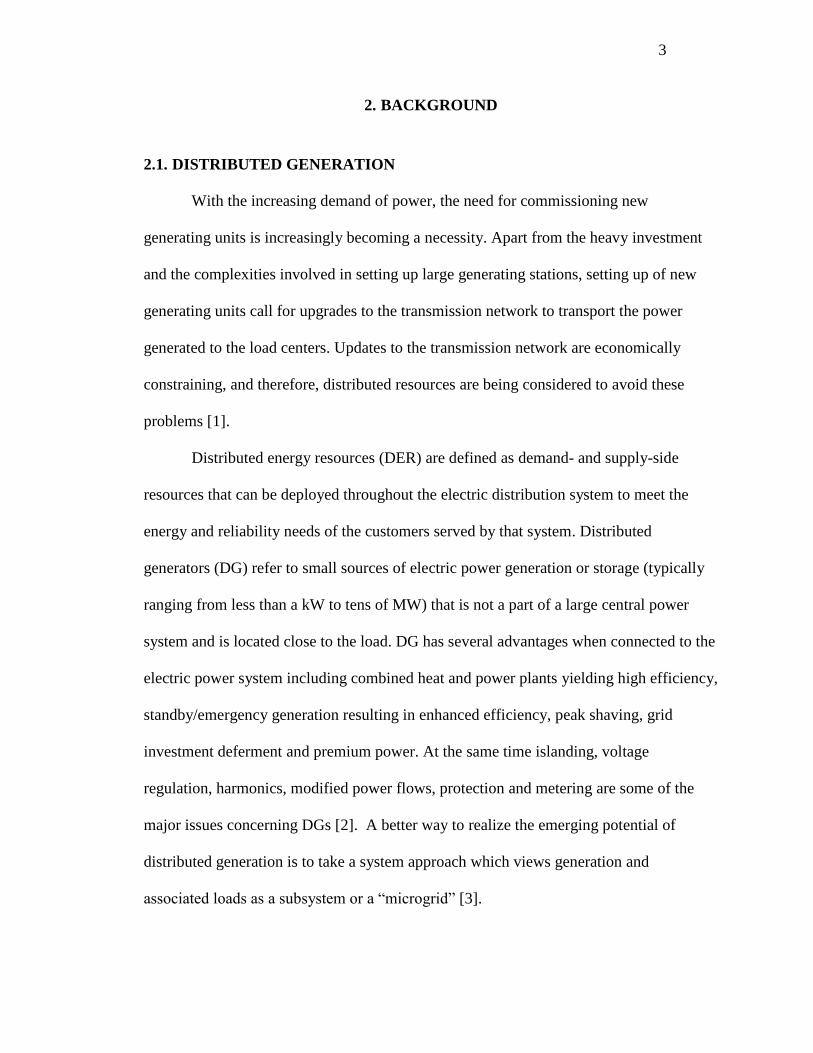
With the increasing demand of power, the need for commissioning new
generating units is increasingly becoming a necessity. Apart from the heavy investment
and the complexities involved in setting up large generating stations, setting up of new
generating units call for upgrades to the transmission network to transport the power
generated to the load centers. Updates to the transmission network are economically
constraining, and therefore, distributed resources are being considered to avoid these
problems [1].
Distributed energy resources (DER) are defined as demand- and supply-side
resources that can be deployed throughout the electric distribution system to meet the
energy and reliability needs of the customers served by that system. Distributed
generators (DG) refer to small sources of electric power generation or storage (typically
ranging from less than a kW to tens of MW) that is not a part of a large central power
system and is located close to the load. DG has several advantages when connected to the
electric power system including combined heat and power plants yielding high efficiency,
standby/emergency generation resulting in enhanced efficiency, peak shaving, grid
investment deferment and premium power. At the same time islanding, voltage
regulation, harmonics, modified power flows, protection and metering are some of the
major issues concerning DGs [2]. A better way to realize the emerging potential of
distributed generation is to take a system approach which views generation and
associated loads as a subsystem or a “microgrid” [3].
Page 17
4
2.2. MICROGRID
2.2.1. Definition. Microgrids are power systems that can operate autonomously
using combinations of conventional generation technologies such as diesel gensets and
combined heat and power systems, renewable resources, other new generation
technologies, such as micro-turbines and fuel cells, energy storage systems, and load
management systems. In many ways, a microgrid is really just a small-scale version of
the traditional power grid that the vast majority of electricity consumers in the developed
world rely on for power service today. IEEE Std. 1547.4-2011 [4] defines DER island
systems or microgrids as electric power systems (EPS) that: have DER and load, have the
ability to disconnect from and parallel with the area EPS, include the local EPS and may
include portions of the area EPS and are intentionally planned.
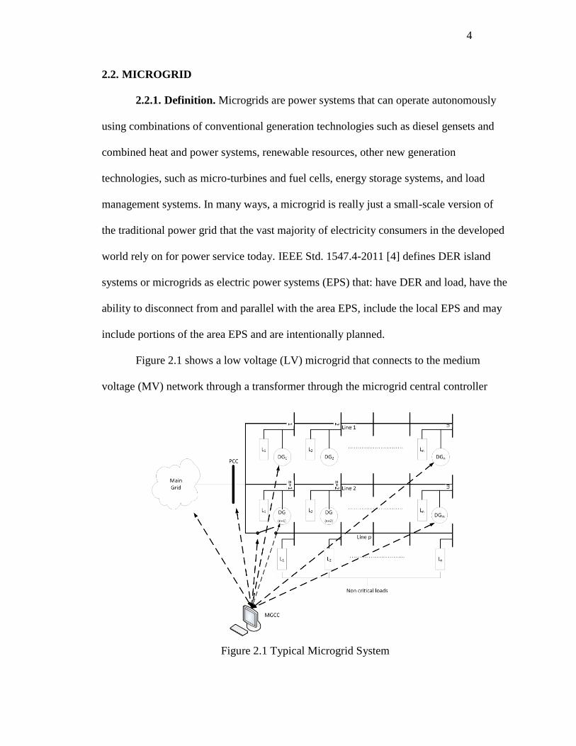
Figure 2.1 shows a low voltage (LV) microgrid that connects to the medium
voltage (MV) network through a transformer through the microgrid central controller
Figure 2.1 Typical Microgrid System
Page 18
5
(MGCC) at the point of common coupling (PCC). The microgrid comprises of various
DGs such as CHP, PV and microturbines, and energy storage resources such as batteries
and fuel cells. Every distributed generator is connected to the microgrid through a
microsource controller (MC) and the load is connected through a load controller (LC) [5].
There are several benefits to microgrids [6]. Microgrid is described as a tool for
sustainable energy [7]. Firstly, microgrids facilitate connection of distributed generation
(DG) and high penetration of renewable energy sources. They also facilitate cogeneration
in a combined heat and power (CHP) system [8]. They increase power quality and
reliability of electric supply. They defer network investments. They contribute to
adequacy of generation because of its ability to control internal loads and generation.
They also support the electrical network in remote sites and rural areas [9].
There are also economic benefits from microgrids [10]. Barker, et al [11] have
estimated the cost of power from microgrids with DG support to be 10 ¢/kWh as opposed
to 10.5¢/kWh in the case of conventional power.
The necessity of microgrids can be understood from the article in PEI magazine
[12] which quotes that the vision of DOE for smart grids to improve power quality with
more control and awareness of the operational state of the electric system at affordable
prices cannot be achieved either until the T&D system is fixed or microgrids come into
existence. Venkatramanan et al [13] present a growth model wherein the various features
and barriers for microgrids have been identified.
The other reasons for such recognition for microgrid over recent times have been
because of increased awareness for the environmental concerns and the ever increasing
price for fossil fuels which has resulted in the increased attention towards implementing
Page 19
6
renewables into power systems. Also there is a high priority for countries to have energy
security. All these reasons have increased governments’ interest in microgrids.
At the same time, several obstacles have also been identified for the growth of
microgrids which need to be addressed [4]. Lack of established regulatory policies and a
solid regulatory base in place in the United States is a major hurdle. Pudjianto et al [14]
present a review of the regulatory situation in Netherlands, United Kingdom and Spain.
At the same time there are certain legal issues, such as the Public Utility Holding
Company Act (PUHCA) in the United States which mandates that sale of electricity for
resale in interstate commerce would turn the seller into a public utility and require filings
with the Securities and Exchange Commission (SEC) and the Federal Power Commission
(FPC). Also, King [15] presents results of a survey involving the staff representing 26
different state PUCs and the PUC of the district of Columbia concerning the legality of
microgrids, interaction between microgrids and utilities and regulatory oversight of
microgrids and microgrid firms.
2.2.2. Modes of Operation. Four modes of operation have been identified by
IEEE Std. 1547.4-2011 [4], namely: area grid connected mode, transition-to-island mode,
island mode, and reconnection mode.
In the grid connected mode, it is advised that the Measuring, Information
exchange and Control (MIC) equipment needs to be in operation to make system related
information available including protection device status, generation levels, local loads,
and system voltages, to the island control scheme such that a transition can be planned in
advance.
During the transition-to-island mode, it is advised that enough DER and DER of
the correct type (DER conforming to all the IEEE Std. 1547.4 [4]) is ensured to be
Page 20
7
available to support the system voltage and frequency for whatever time the island
interconnection device and protective relaying take to effect a successful transition. Also,
if sufficient DER and DER of the correct type are not present, then black start capability
needs to be provided inside the island. Pedrasa, et al [16] identifies some more issues
such as balance between supply and demand, power quality, communication among
microgrid components and micro-source issues like lack of inertia, lack of spinning
reserves and slow response or ramp time.
During the island mode, it is suggested that one or more participating DER will
need to be operated outside the IEEE 1547 voltage regulation requirement to assure DER
island system voltage and frequency stability. Also, there should be adequate reserve
margin that is a function of the load factor, the magnitude of the load, the load shape, the
reliability requirements of the load, and the availability of DER. It is suggested that to
balance the load and the generation within the island various techniques such as load-
following, load management, and load shedding be used. Also, it is pointed out that
transient stability should be maintained for load steps, DER unit outage, and island faults.
It is also suggested that adaptive relaying may be implemented to provide adequate
protection for a variety of system operating modes. Bollen, et al [17] propose standard
operating ranges for frequency and voltage based on the European standard EN50160 for
interconnected and islanded systems. It is proposed that for interconnected systems, the
frequency shall be between ±5 Hz during 99.5% of the year and always between -3 and
+2 Hz of the nominal frequency. For islanded systems, the frequency shall be always
between ±1 Hz during 95% of one week and always between ±7.5 Hz. The voltage for
island operation lasting less than 10 minutes shall be between 85% and 110% of the
declared voltage.
Page 21
8
For reconnection of the DER island system to the EPS, monitoring should
indicate that the proper conditions exist for synchronizing the island with the EPS. It is
advised that after an area EPS disturbance, no reconnection shall take place until the area
EPS voltage is within Range B of ANSI/NEMA C84.1-2006, Table 1, the frequency
range is between 59.3 Hz to 60.5 Hz, and the phase rotation is correct. Also, the voltage,
frequency, and phase angle between the two systems should be within acceptable limits
as specified in IEEE Std 1547-2003 in order to initiate a reconnection. Several ways to
reconnect the DER island system back to the EPS are also mentioned.
2.3. SYNCHRONOUS MACHINE BASED MICROSOURCES
2.3.1. Necessity of Synchronous Machine Based Microsources. Synchronous
machine have been used as generators for several decades in the power system. Most of
the generations today are from three phase synchronous generators. Several advantages of
synchronous machines have ensured the dominance of synchronous generators.
Being inertia based, synchronous machines can maintain synchronism from
transient oscillations in the system. With appropriate controls in place, synchronous
machines can also ensure that there is a balance of demand and supply in the system.
They also have the inherent nature of operating at constant frequency. Being excited by
an external DC excitation source, synchronous machines can be operated at both leading
and lagging power factor. Hence, they can be used to also generate reactive power
required by the system or they can be used to absorb excess reactive power and hence
improve the voltage profile in the system.
Synchronous machine-based DG are normally used for combined heat and power
applications [18]. Combined heat and power systems have very high energy efficiency
Page 22
9
and reduce energy costs. Thus it is very beneficial to include synchronous machine based
DGs in the microgrid.
2.3.2. Control of Synchronous Machine Based Microsources. The control
system of the synchronous machines needs to ensure that the synchronous machine
generates active and reactive power within the ratings of the machine at nominal voltage
and frequency as demanded by the system to which it is connected. At the same time the
load in the system has to be served and the machines must each generate a share of the
power demanded by the load.
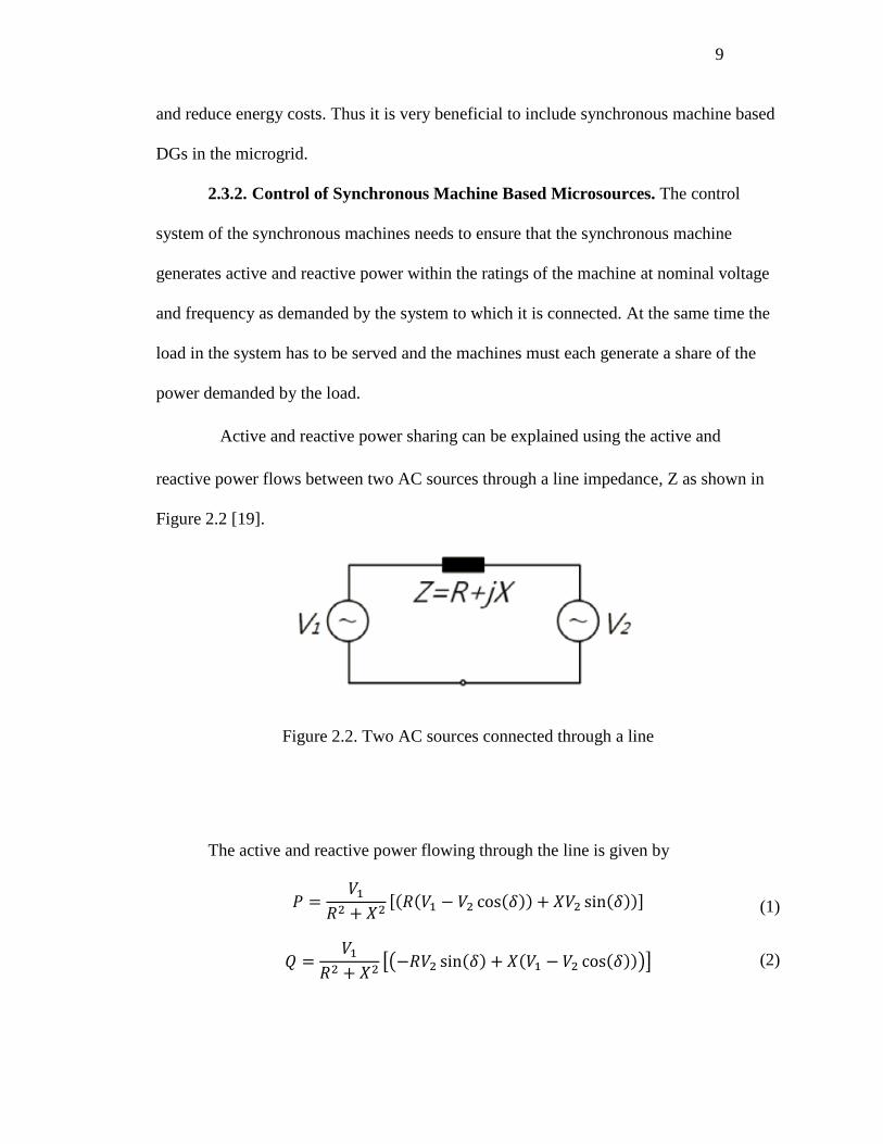
Active and reactive power sharing can be explained using the active and
reactive power flows between two AC sources through a line impedance, Z as shown in
Figure 2.2 [19].
Figure 2.2. Two AC sources connected through a line
The active and reactive power flowing through the line is given by
[( ( ( )) ( ))] (1)
[( ( ) ( ( )))] (2)
Page 23
10
For a predominantly inductive line, the phase angle between the two voltages is
very small. Hence for small δ,
( ) (3)
( ) (4)
Thus, the active power is proportional to the phase angle and the reactive power is
proportional to the voltage difference between the two systems. Hence, a DG can control
its active power by controlling the frequency at which it is generating and the reactive
power by controlling the voltage at its terminal.
From the synchronous machines view point, two inputs that can be used as control
parameters are torque applied by the prime mover to the shaft of the machine and the
voltage across the field winding of the synchronous machine. The torque applied controls
the speed of the shaft affecting the frequency of the power generated by the machine, and
hence, the active power generated by the machine. The field voltage controls the terminal
voltage, and hence, the reactive power generated by the machine.
Page 24
11
3. SYNCHRONOUS MACHINE CONTROLLER DESIGN
In a microgrid environment, the synchronous machine will be required to operate
in different scenarios or modes. In the grid connected mode, the machine is connected to
an infinite bus such as the EPS, and the voltage and frequency are no longer the control
objectives of the machine control system, and remain fixed irrespective of the torque and
the field voltage applied. Thus, we need to use the shaft torque and the field voltage as
tools to modulate the output active and reactive powers of the machine. In the islanded
mode, it will be the responsibility of the control system to ensure nominal voltage and
frequency apart from delivering the required amount of power to the system. Thus
depending on the mode of operation of the microgrid, the control system for the
synchronous machine will have to change its control strategy to fulfill the needs of the
operating mode.
3.1. CONTROL STRATEGY DURING DIFFERENT MODES OF OPERATION
3.1.1. Control During Islanded Mode – Droop Control. During islanded mode,
the objective is to ensure that the required amount of power is delivered at the nominal
voltage and frequency. It is also important to ensure that the machines in the microgrid do
not loose synchronism. Also, when multiple synchronous generators are present in the
system, there should be a provision for sharing the power demanded by the load taking
the machine ratings into consideration.
Typically frequency is reduced or "drooped" with increasing generated active
power and voltage is drooped with increasing generated reactive power. Droop control
has been extensively used with synchronous machines when multiple synchronous
machines are supplying power and need to maintain nominal voltage and frequency
Page 25
12
within the entire system. In the context of microgrids, since we need to control both the
active and reactive power, two different droop controls need to be used. The first one
being active power-frequency droop (P/ω droop) and the second one being, reactive
power-voltage droop (Q/V droop) [20–24].
First, let us consider a single machine serving a load as shown in Figure 3.1. A
prime mover PM is driving the shaft of a synchronous machine SM which is connected to
a load. As described above, the shaft torque and field voltage have to be used to control
the synchronous machine such that the machine serves the load at nominal voltage and
frequency. According to the theory of droop control, Equations (5) and (6) can be used to
calculate the commanded shaft speed and terminal voltage from the active (Pgen) and
reactive (Qgen) power being generated by the machine. Dpf and DQV are the droop
coefficients for the active and reactive power droop curves. ωrm0 and Vs0 are the speed
and the terminal voltage at no load. They also represent the base speed and terminal
voltage of the machine. Pgen,rated and Qgen,rated are the rated active and reactive power of the
machine.
SM
Load
Figure 3.1. Single generator serving a load
PM
Page 26
13
(
) (5)
(
) (6)
The variation of speed with the active power generated by the machine can be
represented by a straight line according to Equation (5) as shown in Figure 3.2 (a). The
slope of the line is the droop coefficient Dpf. It can be seen that at no load, the machine
operates at rated speed. Once the machine starts to serve load the speed starts decreasing.
Similarly, the variation of terminal voltage with the reactive power generated by
the system can also be represented by a straight line according to Equation (6) as shown
in Figure 3.2 (b). The slope of this characteristic is the droop coefficient DQV.
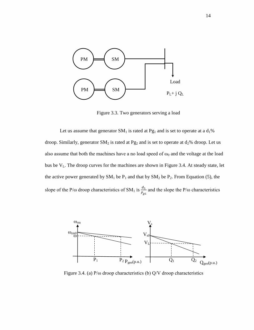
Now let us consider the situation where there are multiple machines in the system.
Let us consider a system where two machines are connected in parallel to a bus as shown
in Figure 3.3.
Vs
Vs0
Pgen(p.u.)
ωrm0
ωrm
Qgen(p.u.)
Figure 3.2. (a) P/ω droop characteristics (b) Q/V droop characteristics
Page 27
14
Let us assume that generator SM1 is rated at Pg1 and is set to operate at a d1%
droop. Similarly, generator SM2 is rated at Pg2 and is set to operate at d2% droop. Let us
also assume that both the machines have a no load speed of ω0 and the voltage at the load
bus be VL. The droop curves for the machines are shown in Figure 3.4. At steady state, let
the active power generated by SM1 be P1 and that by SM2 be P2. From Equation (5), the
slope of the P/ω droop characteristics of SM1 is
and the slope the P/ω characteristics
Load
PL+ j QL
Figure 3.3. Two generators serving a load
SMPM
SMPM
Vs
Vs0
Pgen(p.u.)
ωrm0
ωrm
Qgen(p.u.)
Figure 3.4. (a) P/ω droop characteristics (b) Q/V droop characteristics
P1 P2
ω
VL
Q1 Q2
Page 28
15
of SM2 is
. The active power load being served by both the machines is PL. Since the
frequency at all points in an electrical system has to remain the same, the shaft speed of
both the machines will have to remain the same, say ω.
Thus,
(7)
(
)
(8)
(
)
(9)
[(
)
(
)] (10)
Hence, the share of the active power load generated by each machine can be calculated
as,
(
⁄
⁄
) (11)
Equations (9) and (7) can be used to study the effect of generator rating and droop
coefficient on the share of load generated by each machine. Figure 3.5 and Figure 3.6
show the variation of share of generation by the machine with varying generator ratings
and droop coefficients. The following observations can be made from the graphs.
1. The machine with higher rating generates a higher share of the power demanded.
2. The machine with lower droop coefficient generates a higher share of the power.
Page 29
16
0
10
20
30
40
50
60
70
80
90
0 0.5 1 1.5 2 2.5 3 3.5
Pe
rce
nta
ge o
f ac
tive
po
we
r d
raw
n b
y lo
ad b
ein
g ge
ne
rate
d
Ratio of rating of SM1 to SM2
P1
P2
0
10
20
30
40
50
60
70
0.5 0.75 1 1.25 1.5 1.75
Pe
rce
nta
ge o
f ac
tive
po
we
r d
raw
n b
y lo
ad
be
ing
gen
era
ted
Ratio of droops of SM1 to SM2
P1
P2
Since both generators are connected to the same bus, the share of reactive power
is similar to that of the active power. But such a system might not be practically feasible
Figure 3.5. Variation of share of generation with generator ratings assuming equal droop
Figure 3.6. Variation of share of generation with droop assuming equal ratings
Page 30
17
in the real world. The generators may have to be separated by some physical distance
leading to a line connecting the two machines.
3.1.2. Control During Grid Connected Mode. During grid connected mode the
objective of the synchronous machine controller is to control constant output power.
Since the frequency is determined by the grid and is held stiff, the rotor speed is constant.
As a result the power output depends directly on the torque exerted by the prime mover
on the shaft. Thus the mode of operations is referred to as Constant Power Mode (CPM).
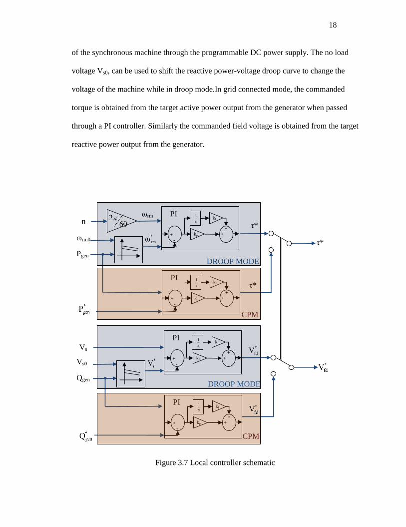
3.2. LOCAL CONTROLLER DESIGN
The local controller is responsible for maintaining stable operation of the
generating units. As shown in Figure 3.7, the local controller will have to use the stator
voltages, line currents and shaft speed to decide the commanded torque, τ* and
commanded field voltage, Vfd*. As explained earlier, the local controller will have to
switch between constant power mode for grid connected operation and droop mode for
islanded operation.
Using the stator voltages and currents, active and reactive powers delivered by the
DG is calculated. In the droop mode, the commanded torque is calculated from the active
power being generated by the machine, Pgen. Active power is passed through a droop
control block. The droop control block is also fed with the no-load speed as an input. This
input is used to shift the droop curves as explained earlier. The droop controller
calculates the target shaft speed, ωrm which is given to a PI controller which converts the
target shaft speed to a commanded torque, τ*. The DC machine is commanded to apply
this torque on the shaft through the DC machine drive. Similarly the reactive power being
generated is used to calculate the field voltage required to be applied to the field winding
Page 31
18
of the synchronous machine through the programmable DC power supply. The no load
voltage Vs0, can be used to shift the reactive power-voltage droop curve to change the
voltage of the machine while in droop mode.In grid connected mode, the commanded
torque is obtained from the target active power output from the generator when passed
through a PI controller. Similarly the commanded field voltage is obtained from the target
reactive power output from the generator.
Figure 3.7 Local controller schematic
+
-
𝑠
+ +
kI
kp
PI
+
-
𝑠
+ +
kI
kp
PI
ωrm0
Pgen
ωrm
n
τ*
τ*
τ*
+
-
𝑠
+ +
kI
kp
PI
+
-
𝑠
+ +
kI
kp
PI
Vs0
Qgen
Vs
DROOP MODE
DROOP MODE
CPM
CPM
Page 32
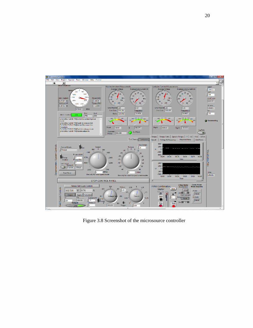
19
A screenshot of the LabVIEW interface for the local controller is shown in Figure
3.8. The drive conditions panel on the top-right shows the speed, armature and field
currents, power drawn and the torque applied on the shaft of the DC machine drive.
Below the drive conditions panel is the MGCC panel where MGCC control can be
enabled/disabled. If the MGCC control is disabled, the operator can control the DG by
selecting the mode of operation (Droop/CPM), and the commanded active and reactive
powers. Pset and Qset display the set points received from MGCC. A list of all messages
received with the date and time stamp is also recorded here. Machine armature
measurements and contactor terminal measurements panels display the measured voltage,
current and frequency. Active, reactive and apparent powers are calculated and displayed.
The Dynamometer/System Controls panels enables the operator to operate the DG
manually. For MGCC control, the control mode has to be set to Torque. The droop
control panel ensures the speed of the shaft obtained from the active power-frequency
droop equation. The Visualization Tabs plot speed, torque, active and reactive power,
voltage, frequency and grid power flows vs. time. The field supply controls panel
controls the programmable power supply. When the output is turned on and the Q~V
droop is enabled, field voltage corresponding to the reactive power-voltage droop
equation is commanded. The FVNR combination starter panel has controls to the
contactors connected to the DG.
Page 33
20
Figure 3.8 Screenshot of the microsource controller
Page 34
21
4. MICROGRID CENTRAL CONTROLLER
4.1. RESPONSIBILITIES OF THE MGCC
Microgrids can comprise of several DGs which can be located at a distance from
each other. There is a need for maintaining coordinated operation and control of all the
DGs in the microgrid to maintain stability in the system and accomplish the goals of the
microgrid [25]. Thus, there is a need for a supervisory controller which coordinates the
operation of the local microsource controllers through a communication network. The
supervisory controller or the microgrid central controller (MGCC) can receive status
information from all the local controllers and monitoring systems in the microgrid and
take decisions from a system point of view.
The importance of having a centralized controller like the MGCC is described in [26–
29]. Some of the key facts are noted based on the literature review:
To provide power set points for the DGs
To ensure economic scheduling
To supervise demand side bidding
To control peak load during peak load hours
To control non critical loads during islanding
To minimize system loss
To detect islanding conditions based on the point of common coupling (PCC)
measurements
To provide LC with the information when grid comes back for
resynchronization
To monitor power flow through local generating units and PCC
Page 35
22
The MGCC can be very beneficial for managing the overall stability of the
microgrid. Decisions such as when to island the microgrid can be crucial for the
operation of the microgrid. It is important that all the microsource controllers take action
on these decisions simultaneously. If such decisions are taken by the local controllers
themselves then coordinated operation cannot ensured.
Figure 4.1 describes the various functionalities that the MGCC can provide for the
microgrid. Since the MGCC can monitor the point of common coupling (PCC), the
MGCC can analyze the power quality at the PCC and decide to island the microgrid.
Islanding decisions can also be dependent on economic considerations as well. Also, the
MGCC can monitor power being generated by the renewable energy sources and
optimize the power generated by other sources. Further, the MGCC can keep a record of
the power flows and system conditions from the past, and use those records to forecast
the load and plan the generation within the microgrid ahead of time, especially when real
time pricing of power is in place. For example if the MGCC can predict that there will be
Figure 4.1 Microgrid Central Controller responsibilities
MGCC
Islanding Detection
Resynchr-onizing to the grid
Planning and
Operation
Back up Protection
Load Shedding
Data Logging
Page 36
23
an increase in demand for power after a certain time, then the batteries in the system can
be charged when the cost of energy is cheap and use that energy when the demand picks
up. If need be, the MGCC can decide to shed some load to ensure stable and economic
operation of the microgrid [30].
The MGCC can also be used for back up protection within the microgrid. Direct
connected rotating machines can be prone instability during voltage dips caused by faults
in island-operated microgrid, and therefore, they may jeopardize the stability of the entire
microgrid [31]. Since the MGCC is in constant communication with the entire microgrid,
it can also be used as a backup protection scheme of the microgrid.
After islanding, once the grid support is restored, and it is decided to reconnect,
the voltage and frequency at the PCC will have to be matched with that on the grid side.
The MGCC can coordinate with multiple local controllers to instruct them to regulate
their voltage and frequency to facilitate resynchronization with the grid.
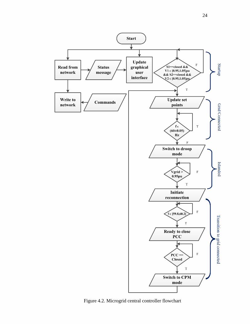
4.2. MGCC ALGORITHM DEVELOPMENT
In this study, the MGCC is used to make islanding decisions and during
resynchronization with the grid. Primarily, the MGCC has to be in constant
communication with the various MCs and LCs in the system. It receives status data from
the DGs, the switches, and other measurement units in the system. In the second process,
the status data are studied and commands are generated for the microsource controllers
and transmitted back to them. A flow chart for the MGCC is presented in Figure 4.2.
Page 37
24
Figure 4.2. Microgrid central controller flowchart
Page 38
25
The MGCC operating flow chart has four different objectives. These are:
1. Startup
Start DG units and synchronize them to their corresponding buses.
Track synchronization of the DGs
2. Grid connected operation
Monitor PCC voltage and frequency
Send active and reactive power set points to the local controllers
Monitor islanding condition
3. Islanded
Command local controllers to go to droop mode
Shed non critical load
Monitor PCC voltage and frequency
Initiate transition to grid once the grid is back
4. Transition to grid connected
These operating modes are described below:
During startup, the MGCC starts communicating with the local controllers, the
PCC and non-critical load breakers. It checks if the PCC voltage is within the range of
1.05 pu to 0.95 pu as well as PCC breaker is on or off. Parallel to this event, the MGCC
checks the terminal voltage of the newly started DG unit and the status of the contactor,
which connects DG with the microgrid.
During grid connected mode, the MGCC commands the local controller to
generate specific amounts of active and reactive power from its associated DG. At the
same time, the MGCC checks if the system frequency is within ±5% of 60Hz and
Page 39
26
monitors the grid side PCC voltage. If the system frequency is not within this band, the
MGCC switches to islanded mode of operation.
During islanded mode, the MGCC sends a message to the local controllers to
switch to droop mode. The MGCC continues monitoring the grid side PCC voltage and
frequency. As soon as the MGCC finds that PCC side grid voltage and frequency is
restored to the nominal value, it sends a message to the local controller to initiate
reconnection.
Local controller receives signal from the MGCC and immediately responds to the
mode by shifts the droop curve in such a way as to match the grid side frequency which is
60Hz. At the same time, the MGCC sends the information of the PCC voltage to the DGs
so that, they can start to increase or decrease their terminal voltage until the microgrid
side PCC voltage matches with the grid side PCC voltage. At this point The MGCC
closes the PCC contactor between the microgrid and the main grid. As soon as the
contactor is closed, the MGCC sends a signal to the local controllers to switch to constant
power mode. The MGCC then switches to grid connected mode.
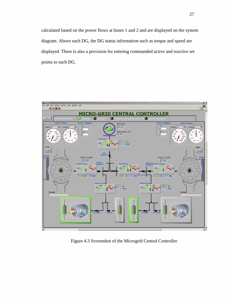
4.3. IMPLEMENTING THE MICROGRID CENTRAL CONTROLLER
The MGCC has a graphical user interface platform which shows status of the
microgrid. A screenshot of the MGCC is shown in Figure 4.3. On the top of the MGCC,
the current operating mode of the MGCC is defined. An interactive system diagram
shows the system status information. LED indicators are provided for the grid, and the
DGs to show their participation in the microgrid. Grid voltage, frequency, DG voltages
and active and reactive power flows are displayed as received from their respective MCs.
Contactor/switch states are also displayed on the system diagram. Load states are
Page 40
27
calculated based on the power flows at buses 1 and 2 and are displayed on the system
diagram. Above each DG, the DG status information such as torque and speed are
displayed. There is also a provision for entering commanded active and reactive set
points to each DG.
Figure 4.3 Screenshot of the Microgrid Central Controller
Page 41
28
5. LABORATORY MICROGRID TEST SYSTEM
5.1. MICROGRID SYSTEM DESIGN
The laboratory microgrid test system comprises of two generating units (DGs).
Each DG is connected to the microgrid through a contactor/switch to connect/disconnect
from the microgrid. The system is a three bus system. As shown in Figure 5.1, DG1 is
connected to bus 1, DG2 to bus 2 and grid to bus 3. Detailed discussion on the DGs is
presented in Section 5.2. Utility grid is stepped down to 230V, the rating of the DGs and
the loads and is supplied to the PCC, bus 3, through a contactor to facilitate islanding.
Buses 1 and 2 are connected to bus 3 through two lines 1 and 2. Resistive and resistive
inductive loads are connected to buses 1 and 2.
Figure 5.1. The laboratory microgrid system
Page 42
29
A computer equipped with LabVIEW® software and NI PCI 6221 data acquisition
card acts as a local controller which commands torque and field voltage to the DC
machine drive and the power supply respectively. The rating of various pieces of
equipment is listed in Table 5.1.
Table 5.1 Laboratory equipment ratings
Equipment Parameter Rating Units
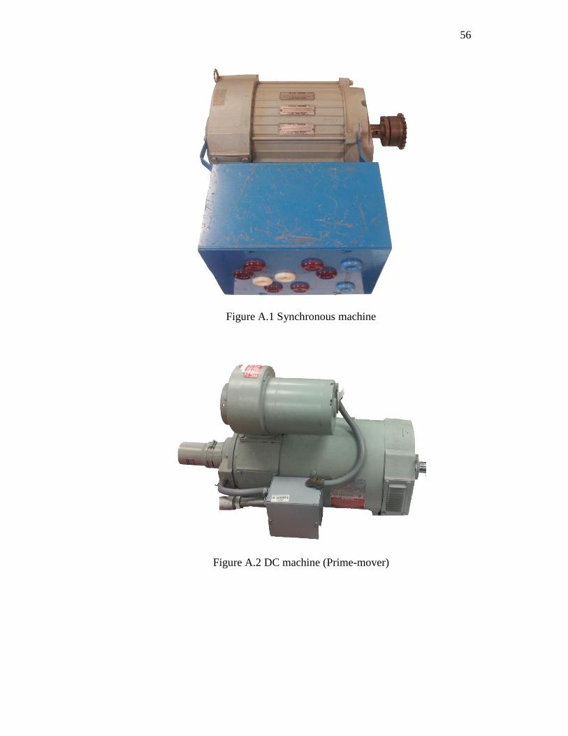
Synchronous
Machine
Voltage 230/460 Volts
Current 6.28/3.14 Amps
Power 2.5 kVA
Power Factor 0.8 lagging
Field Voltage 150 Volts
Field Current 1.05 Amps
DC Machine
Voltage 240 Volts
Current 70.5 Amps
Power 20 HP
Field Voltage 150 Volts
Field Current 2.7/1.3 Amps
Speed 1750/2700 Rpm
DC Machine
Drive
Input Voltage 3-230...500 Volts
Input Current 114 Amps
Input frequency 50-60 Hz
Output Voltage 240...500 Volts
Output Current 140 Amps
Field Current 6 Amps
Programmable
DC power
supply
Input Voltage 115-230 Volts
Input Current 11/6 Amps
Input Phases 1 Phase
Input Frequency 50-60 Hz
Output Voltage 0-300 Volts
Output Current 0-2 Amps
Page 43
30
5.2. MICROSOURCES
A block diagram of the generating units is shown in Figure 5.2. Each generating
unit is a three-phase synchronous machine. The shaft of the synchronous machine is
coupled to that of a DC machine. The DC machine represents a prime mover like an
engine. The torque applied by the DC machine on the shaft is analogous to the fuel valve
opening in an engine. The DC machine is controlled by a Saftronics DC400 drive. The
drive is responsible for producing field and armature currents required by the machine to
ensure that the commanded torque τ* is applied to the shaft by the DC machine. The field
winding of the synchronous machine is supplied by a Sorensen programmable power
supply which emulates an exciter. The power supply is responsible for supplying the
commanded field voltage to the field winding of the synchronous machine. Both the
Saftronics DC400 drive and the Sorensen programmable power supply are controlled by
the MC over Ethernet.
DC
PROGRAMMABLE
DC POWER
SUPPLY
+DC -DC
3Φ
su
pp
ly
3Φ supply
Vfd*τ*
LOCAL
CONTROLLER
From
MGCC
SM
Wat
tmet
er
V,I
DC
MACHINE
DRIVE
A1
A2
F1
F2
ω
Figure 5.2. Generating Unit Line Diagram
Page 44
31
The wattmeter comprises of three LEM LV 25-P potential transformers and three
LEM LA 55-P current transducers mounted on each phase. These currents and voltages
sensors are connected to the PCI 6221 DAQ’s analog input ports. The frequency and
active and reactive powers are calculated in the MC.
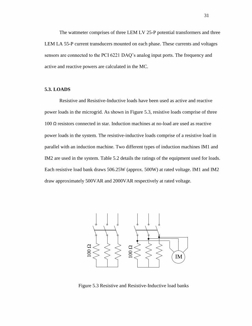
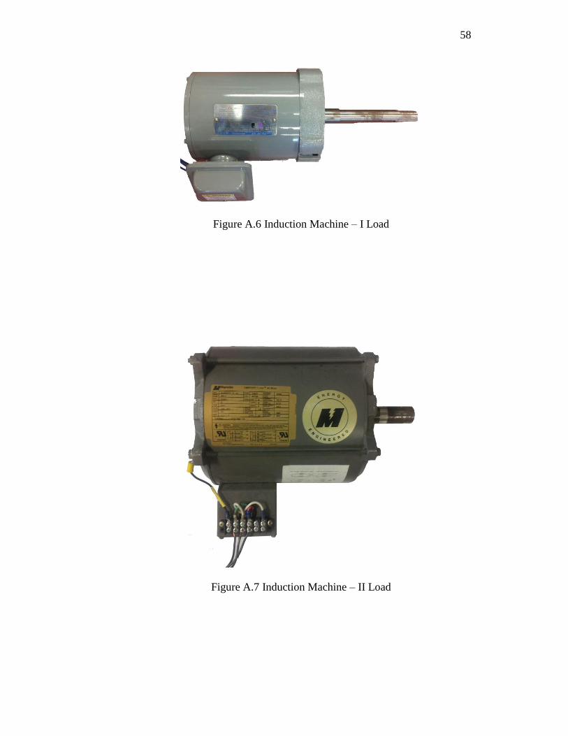
5.3. LOADS
Resistive and Resistive-Inductive loads have been used as active and reactive
power loads in the microgrid. As shown in Figure 5.3, resistive loads comprise of three
100 Ω resistors connected in star. Induction machines at no-load are used as reactive
power loads in the system. The resistive-inductive loads comprise of a resistive load in
parallel with an induction machine. Two different types of induction machines IM1 and
IM2 are used in the system. Table 5.2 details the ratings of the equipment used for loads.
Each resistive load bank draws 506.25W (approx. 500W) at rated voltage. IM1 and IM2
draw approximately 500VAR and 2000VAR respectively at rated voltage.
100 Ω
100 Ω
IM
Figure 5.3 Resistive and Resistive-Inductive load banks
Page 45
32
Buses 1 and 2 are equipped with loads: RL-load-1, RL-load-2, R-Load-1, and R-
Load-2. Each of these loads comprise of several resistive and resistive-inductive loads as
shown in the one-line diagram, Figure 5.4. Table 5.3 lists the calculation of the total
active and reactive power drawn by each of these loads when all the switches are turned
on.
IM1 IM1 IM2
(a) R-load-1 (b) R-load-2 (c) RL-load-1 (d) RL-load-2
Figure 5.4 One-line diagram of the loads in the microgrid
Table 5.2 Load equipment ratings
Equipment Parameter Rating Units
Load Resistor Resistance 100 Ohms
Power 225 Watts
Load IM- I
Voltage 230/460 Volts
Current 2.9/1.5 Amps
Speed 1735 Rpm
Frequency 60 Hz
Power 0.75 HP
Load IM- II
Voltage 230/460 Volts
Current 12.8/8.4 Amps
Speed 1745 Rpm
Frequency 60 Hz
Power 5 HP
Page 46
33
Table 5.3 Loads in the microgrid
Load
No. of
resistive
load
banks
No. of
resistive-
inductive load
banks with
IM1
No. of
resistive-
inductive load
banks with
IM2
Total active
power
demand
(W)
Total
reactive
power
demand
(VAR)
R-load-1 3 0 0 1500 0
RL-load-1 1 1 0 500 500
R-load-2 2 0 0 1000 0
RL-load-2 2 1 1 1000 2500
Total 8 2 1 4000 3000
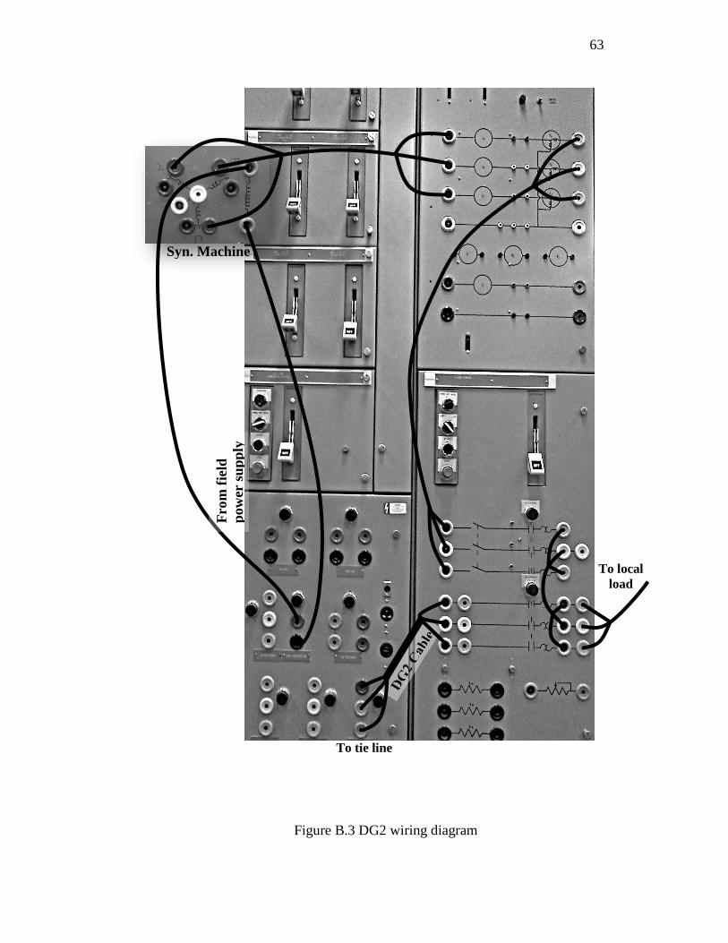
5.4. LINES
Buses 1 and 2 are connected to the point of common coupling with cables. These
cables replicate the distribution lines between different points on a distribution network.
AWG 12 cables are used for the laboratory setup. 153 feet of cable is used between buses
1 and 3 and 156 feet of cable is used between buses 2 and 3. The resistance of the cables
was measured to be 243mΩ and 248mΩ between buses 1 and 3 and buses 2 and 3
respectively.
Page 47
34
6. TEST RESULTS
6.1. MICROGRID OPERATING PROCEDURE
6.1.1. Startup. Initially, it is assumed that the loads within the area of the
microgrid are being served by the grid and the DGs are installed within the microgrid and
are ready to be started. Every DG is assumed to have a switch/breaker which connects it
to a bus within the microgrid. Initially the switch is assumed to be open. The objective of
the startup procedure is to get the DGs started and ready to supply power to the network
when needed.
The following procedure is suggested:
1. Start the prime movers (DC machines in our case) of the synchronous machines.
2. Bring up the speed to 1800 rpm (corresponding to 60 Hz frequency of the grid).
This can be done by running the DG in droop mode. Since the DG is not
connected to the microgrid, the load being served is zero. At no load the DG will
run at 1800 rpm based on the droop characteristics.
3. Apply field voltage such that it is very close to the voltage of the bus to which it is
being connected.
4. The synchronization lamps should be blinking very slowing. Close the contactor
at an instant when all the lamps are off.
5. Switch the DG into constant power mode.
Page 48
35
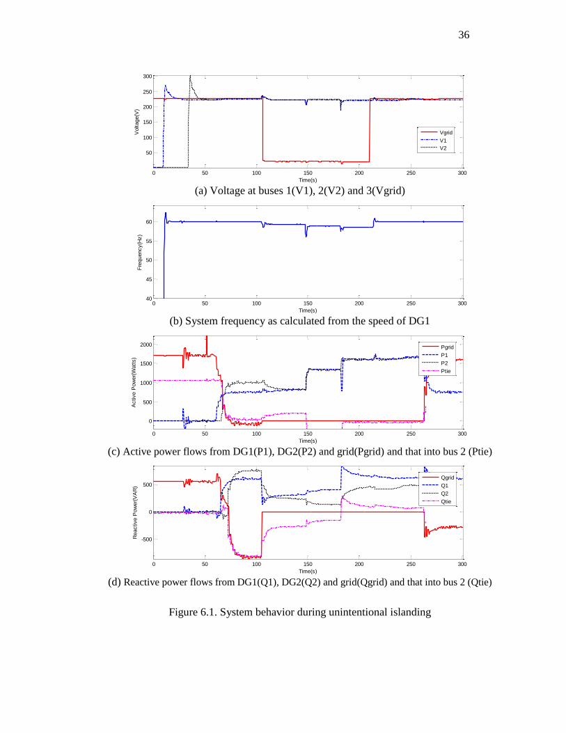
6.1.2. Unintentional Islanding. This is a situation when there is a fault, and the
grid is unable to supply power to the microgrid. Synchronous machine based DGs can be
very valuable in such situations. It is very important that the grid supply be monitored at
all times and once the MGCC decides to island, all the MCs are instructed to switch to
droop mode. Figure 6.1 shows the system behavior during an unintentional islanding test
case. The test procedure is described in Table 6.1.
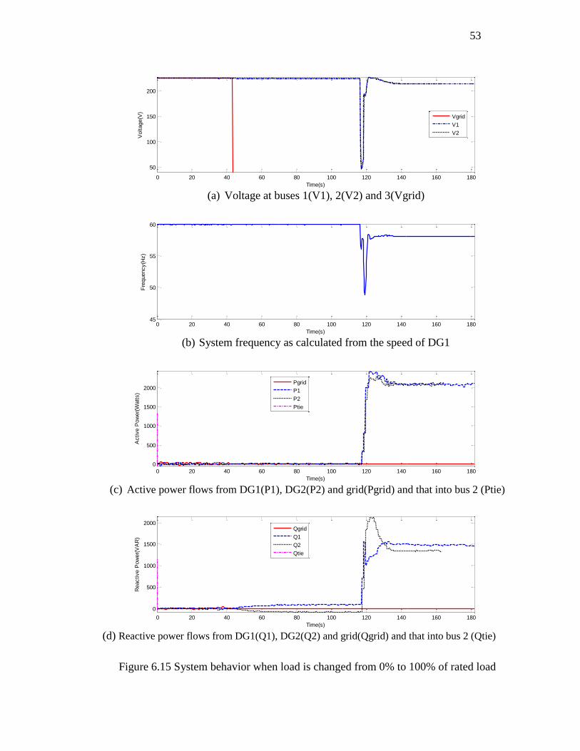
The following observations can be made from these results.
From Figure 6.1 (a) and (b) it is observed that the loads are always served at
nominal voltage and frequency.
From Figure 6.1 (c) and (d), once the both generators are commanded to supply
power, power drawn from the grid decreases. When the system is connected to
grid, the generators participate in serving the load.
From Figure 6.1 (c) and (d), both generators DG1 and DG2 generate active and
reactive powers as demanded by the system. The generators do not lose
synchronism and both generators contribute to the power demanded by the
system. Thus, the system maintains stability during all modes of operation.
At t=145 sec and t=180 sec, the load in the system is changed. This change in
load results in voltage and frequency transients. It can be noticed that the size of
the transient corresponds to the size of load being added. When R-load-1 was
added at t=145sec, there is a very small voltage transient since there is no
considerable amount of reactive load added to the system. But at t=180sec, when
RL-load-2 is added, the voltage transient is much larger. Similar transients can be
observed on the system frequency.
Page 49
36
(a) Voltage at buses 1(V1), 2(V2) and 3(Vgrid)
(b) System frequency as calculated from the speed of DG1
(c) Active power flows from DG1(P1), DG2(P2) and grid(Pgrid) and that into bus 2 (Ptie)
(d) Reactive power flows from DG1(Q1), DG2(Q2) and grid(Qgrid) and that into bus 2 (Qtie)
Figure 6.1. System behavior during unintentional islanding
0 50 100 150 200 250 300
50
100
150
200
250
300
Time(s)
Voltage(V
)
Vgrid
V1
V2
0 50 100 150 200 250 30040
45
50
55
60
Time(s)
Fre
quency(H
z)
0 50 100 150 200 250 300
0
500
1000
1500
2000
Time(s)
Active P
ow
er(
Watt
s)
Pgrid
P1
P2
Ptie
0 50 100 150 200 250 300
-500
0
500
Time(s)
Reactive P
ow
er(
VA
R)
Qgrid
Q1
Q2
Qtie
Page 50
37
(e) Torque commanded to DG1(T1) and DG2(T2)
(f) Field voltage applied to DG1(Vfd1) and DG2(Vfd2)
Figure 6.1. System behavior during unintentional islanding, cont'd.
0 50 100 150 200 250 300
5
10
15
20
time(s)
Com
manded S
haft
Torq
ue(N
.m)
T1
T2
0 50 100 150 200 250 300
120
140
160
180
200
220
time(s)
Fie
ld V
oltage(V
)
Vfd1
Vfd2
Table 6.1 Unintentional islanding procedure
Time(sec) Event
0 Grid is serving a total load of P=1700 W, Q=500 Var.
G1 and G2 are off. S1 and S2 are open.
10 G1 is turned on and brought up to speed and synchronized with bus 1.
50 G2 is turned on and brought up to speed and synchronized with bus 2.
60 G1 is commanded to supply 750 W and 600 Var each.
65 G2 is commanded to supply 1000 W and 650 Var each.
110 Grid voltage is too low. System is islanded.
145 R load is added on station 1
180 RL load is added on station 6
220 Grid voltage is again within acceptable range
275 Microgrid PCC is synchronized with the grid and PCC breaker is closed
Page 51
38
6.1.3. Intentional Islanding. This is a situation when it is decided, a priori, that
the microgrid has to go into islanded mode and there is sufficient time to perform
intentional islanding. One of the possible reasons for this situation can be when the power
quality of the grid is poor and it is decided to switch to islanded mode.
The primary objective is to keep the voltage and frequency dip to a minimum
during transition from grid-connected mode to islanded mode. Thus the following
procedure is suggested:
1. Shed loads which are beyond the total generating capacity of all DGs in the
microgrid. Load shedding can be based on the priority of the load.
2. At the instant after islanding, the power shortage within the microgrid is
equivalent to the amount that the grid was serving before islanding. Thus, based
on machine capabilities and economic considerations, increase generation at some
or all of the DGs in the microgrid such that the power from the grid is negligible.
3. As soon as the power drawn from the grid is negligible, the point of common
coupling for the microgrid can be disconnected and all the machines are switched
to droop mode by the MGCC.
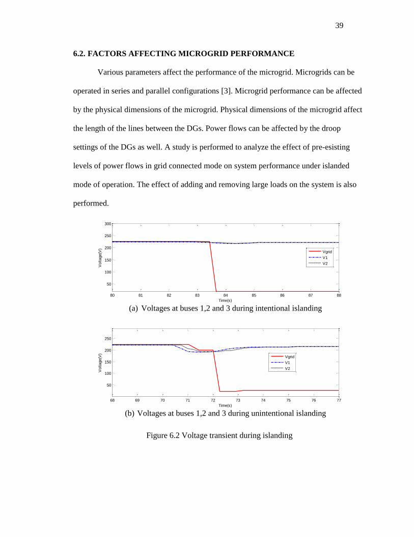
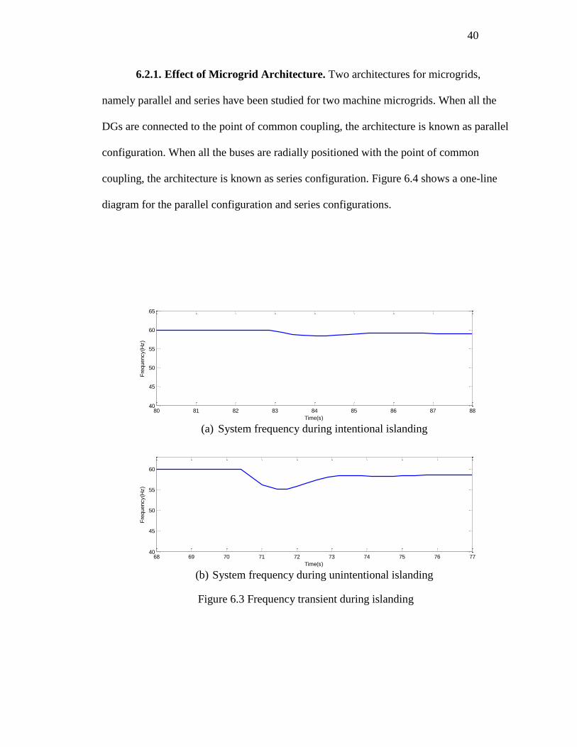
In case of intentional islanding, at the time the point of common coupling is
disconnected from the utility grid, there is no power being drawn from the grid. Hence
the voltage and frequency transients are much smaller when compared to the case of
unintentional islanding. Figure 6.2 and Figure 6.3 compare the voltage and frequency dip
during islanding for both intentional and unintentional islanding situations. Hence the
voltage dip is 4.6 V (2.04%) in the case of intentional islanding as against 33.5 V (14.8%)
during unintentional islanding. The frequency dip is 1.65 Hz (2.75%) during intentional
islanding versus 4.9 Hz (8.16%) during unintentional islanding.
Page 52
39
6.2. FACTORS AFFECTING MICROGRID PERFORMANCE
Various parameters affect the performance of the microgrid. Microgrids can be
operated in series and parallel configurations [3]. Microgrid performance can be affected
by the physical dimensions of the microgrid. Physical dimensions of the microgrid affect
the length of the lines between the DGs. Power flows can be affected by the droop
settings of the DGs as well. A study is performed to analyze the effect of pre-esisting
levels of power flows in grid connected mode on system performance under islanded
mode of operation. The effect of adding and removing large loads on the system is also
performed.
(a) Voltages at buses 1,2 and 3 during intentional islanding
(b) Voltages at buses 1,2 and 3 during unintentional islanding
Figure 6.2 Voltage transient during islanding
80 81 82 83 84 85 86 87 88
50
100
150
200
250
300
Time(s)
Voltage(V
)
Vgrid
V1
V2
68 69 70 71 72 73 74 75 76 77
50
100
150
200
250
Time(s)
Voltage(V
)
Vgrid
V1
V2
Page 53
40
6.2.1. Effect of Microgrid Architecture. Two architectures for microgrids,
namely parallel and series have been studied for two machine microgrids. When all the
DGs are connected to the point of common coupling, the architecture is known as parallel
configuration. When all the buses are radially positioned with the point of common
coupling, the architecture is known as series configuration. Figure 6.4 shows a one-line
diagram for the parallel configuration and series configurations.
(a) System frequency during intentional islanding
(b) System frequency during unintentional islanding
Figure 6.3 Frequency transient during islanding
80 81 82 83 84 85 86 87 8840
45
50
55
60
65
Time(s)
Fre
quency(H
z)
68 69 70 71 72 73 74 75 76 7740
45
50
55
60
Time(s)
Fre
quency(H
z)
Page 54
41
The following points are worth noting in regard to the architectures:
1. In a two DG microgrid system, the positioning of the grid affects the architecture.
If the grid is connected directly to one of the buses then it is a series
configuration. If it is connected between the DGs then it is parallel.
2. If the grid is connected to one of the buses in the system, the bus voltage will
remain stiff during grid-connected mode. Hence given a choice the grid can be
connected to a bus serving any voltage sensitive equipment.
3. In the islanded mode, there is no difference between the configurations.
Figure 6.5 and Figure 6.6 show the similar test results for series and parallel
microgrids. The series microgrid is islanded at t=50sec. Grid voltage is back up at
t=115sec and the microgrid is reconnected at t=125sec. The parallel microgrid is islanded
at t=125sec. Grid voltage is back up at t=95sec and the microgrid is reconnected at
t=135sec. During grid connected mode it can be noticed that both DGs are operating at
the same voltage in the case of parallel microgrid but in case of series microgrid there is a
voltage drop between DG1 and DG2. But this does not affect the voltage or the power
flows during islanded mode.
(a) Parallel configuration (b) Series Configuration
Figure 6.4. Microgrid architecture
Page 55
42
(a) Voltage at buses 1(V1), 2(V2) and 3(Vgrid)
(b) System frequency as calculated from the speed of DG1
(c) Active power flows from DG1(P1), DG2(P2) and grid(Pgrid) and that into bus 2 (Ptie)
(d) Reactive power flows from DG1(Q1), DG2(Q2) and grid(Qgrid) and that into bus 2 (Qtie)
Figure 6.5 Series microgrid system behavior
0 20 40 60 80 100 120 140 160 180200
205
210
215
220
225
230
Time(s)
Voltage(V
)
Vgrid
V1
V2
0 20 40 60 80 100 120 140 160 18050
52
54
56
58
60
Time(s)
Fre
quency(H
z)
0 20 40 60 80 100 120 140 160 180
200
400
600
800
1000
1200
1400
Time(s)
Active P
ow
er(
Watt
s)
Pgrid
P1
P2
Ptie
0 20 40 60 80 100 120 140 160 180
-200
0
200
400
Time(s)
Reactive P
ow
er(
VA
R)
Qgrid
Q1
Q2
Qtie
Page 56
43
(a) Voltage at buses 1(V1), 2(V2) and 3(Vgrid)
(b) System frequency as calculated from the speed of DG1
(c) Active power flows from DG1(P1), DG2(P2) and grid(Pgrid) and that into bus 2 (Ptie)
(d) Reactive power flows from DG1(Q1), DG2(Q2) and grid(Qgrid) and that into bus 2 (Qtie)
Figure 6.6 Parallel microgrid system behavior
0 20 40 60 80 100 120 140
50
100
150
200
Time(s)
Voltage(V
)
Vgrid
V1
V2
0 20 40 60 80 100 120 140
55
56
57
58
59
60
Time(s)
Fre
quency(H
z)
0 20 40 60 80 100 120 1400
500
1000
1500
Time(s)
Active P
ow
er(
Watt
s)
Pgrid
P1
P2
Ptie
0 20 40 60 80 100 120 140
-200
0
200
400
Time(s)
Reactive P
ow
er(
VA
R)
Qgrid
Q1
Q2
Qtie
Page 57
44
6.2.2. Effect of Line Impedance. The length of the lines connecting the DGs to
the PCC determines the impedance between them. During grid connected mode, this
impedance affects the voltage at the DGs. For longer line lengths, the impedance between
the PCC and the DG is large enough causing the voltage to drop significantly. Since the
reactive power depends on the voltage in the droop mode, line impedance can affect the
reactive power sharing between the DGs. Figure 6.7 shows the reactive power and
voltage waveforms when there is no cable connected between the DGs and the PCC. At
t=60sec, the system is islanded. V1 is slightly lower than V2 in islanded mode and as a
result, DG1 generates a higher share of reactive power in comparison to DG2. Reactive
power share is very sensitive to the voltage. For a 5% droop, reactive power generated
increases at a rate of 133.33 Var for a 1V drop in voltage.
(a) Voltage at buses 1,2 and 3 for the test without line impedance
(b) Reactive power flows for the test without line impedance
Figure 6.7 System behavior without line impedance
0 20 40 60 80 100200
205
210
215
220
225
Time(s)
Voltage(V
)
Vgrid
V1
V2
0 20 40 60 80 1000
50
100
150
200
250
300
Time(s)
Reactive P
ow
er(
VA
R)
Qgrid
Q1
Q2
Qtie
Page 58
45
Figure 6.8 shows the reactive power and frequency waveforms for a system with
all the cable (300 feet) between buses 2 and 3. As a result of the impedance of the cable
(490mΩ), the voltage at Bus 2 drops below the voltage at Bus 1. At t=40sec, the system is
islanded. Thus the reactive power generated by DG2 is higher than that generated by
DG1 during islanded mode.
(a) Voltage at buses 1,2 and 3 for the test with line impedance
(b) Reactive power flows for the test with line impedance
Figure 6.8 System behavior with line impedance
0 10 20 30 40 50 60 70 80 90 100200
205
210
215
220
225
Time(s)
Voltage(V
)
Vgrid
V1
V2
0 10 20 30 40 50 60 70 80 90 1000
50
100
150
200
250
300
350
Time(s)
Reactive P
ow
er(
VA
R)
Qgrid
Q1
Q2
Qtie
Page 59
46
6.2.3. Effect of Droop Setting. Droop settings impact the share of power being
generated by a generating station. Higher droop percentages will result in steep droop
characteristics decreasing the share of power generated by the DG. Figure 6.9 shows the
frequency and active power waveforms for a system operating on different active power-
frequency droop percentages. DG1 is operating on 3% droop and DG2 is operating on
5% droop. As a result, DG1 generates more active power than DG2 during islanded
mode. Hence, the active power generated by DG1 exceeds that of DG2 after the system is
islanded at t=37sec.
(a) System frequency as calculated from the speed of DG1
(b) Active power flow measurements from DG1, DG2, grid and tie line
Figure 6.9 Frequency and active power waveforms for DGs operating on different active
power - frequency droop percentages
0 20 40 60 80 100 120 140 16050
52
54
56
58
60
Time(s)
Fre
quency(H
z)
0 20 40 60 80 100 120 140 1600
200
400
600
800
1000
1200
1400
Time(s)
Active P
ow
er(
Watt
s)
Pgrid
P1
P2
Ptie
Page 60
47
Figure 6.10 shows the reactive power and voltage waveforms when DG1 is
operating on a 5% reactive power droop and DG2 is operating on a 3% reactive power
droop. It can be observed that DG2 generates more reactive power. Hence, the reactive
power generated by DG2 exceeds that of DG1 after the system is islanded at t=37sec.
(a) Voltage at buses 1,2 and 3
(b) Reactive power flows measurements from DG1, DG2, grid and tie line
Figure 6.10 Frequency and active power waveforms for DGs operating on
different reactive power - voltage droop percentages
6.2.4. Effect of Grid Connected Generation on Droop Mode Power Sharing.
When the microgrid transitions from grid connected mode to islanded mode, MC changes
from constant power mode to droop mode. Depending on how much power was
commanded from the DGs in the system, the output active and reactive powers can have
a sudden increase or a decrease. Four different tests are conducted on the microgrid
system which are described below. In all the cases the load in the system is held constant
0 20 40 60 80 100 120200
205
210
215
220
225
Time(s)
Voltage(V
)
Vgrid
V1
V2
0 20 40 60 80 100 1200
100
200
300
400
500
600
Time(s)
Reactive P
ow
er(
VA
R)
Qgrid
Q1
Q2
Qtie
Page 61
48
at 1500W and 500VAR measured at rated voltage. Since the load is constant impedance,
the power consumed varies with voltage. The trajectory of the operating point is plotted
on the droop curve for a period of 10 seconds around the time of islanding.
1. An unintentional islanding case when there is a power deficit in the system at
the instant of islanding. Figure 6.11 (a) and (b) show the transition of DG1
and DG2 from grid connected to islanded mode during this case. Both DG1
and DG2 are generating 500 W and 500 VAR before islanding. After
islanding the system stabilizes around 850W from both DG1 and DG2, and
960 Var from DG1 and 850 Var from DG2.
Figure 6.11 (a) DG1 transition to islanded mode for unintentional islanding with power
deficit
Figure 6.11 (b) DG2 transition to islanded mode for unintentional islanding with power
deficit
Page 62
49
2. An intentional islanding case when DG1 is generating 850 W and 950 Var and
DG2 is generating 850 W and 850 VAR. Figure 6.12 (a) and (b) show the
transition of DG1 and DG2 from grid connected to islanded mode during this
case. Even in this case, after islanding the system stabilizes around 850 W
from both DG1 and DG2, and 960 Var from DG1 and 850 Var from DG2.
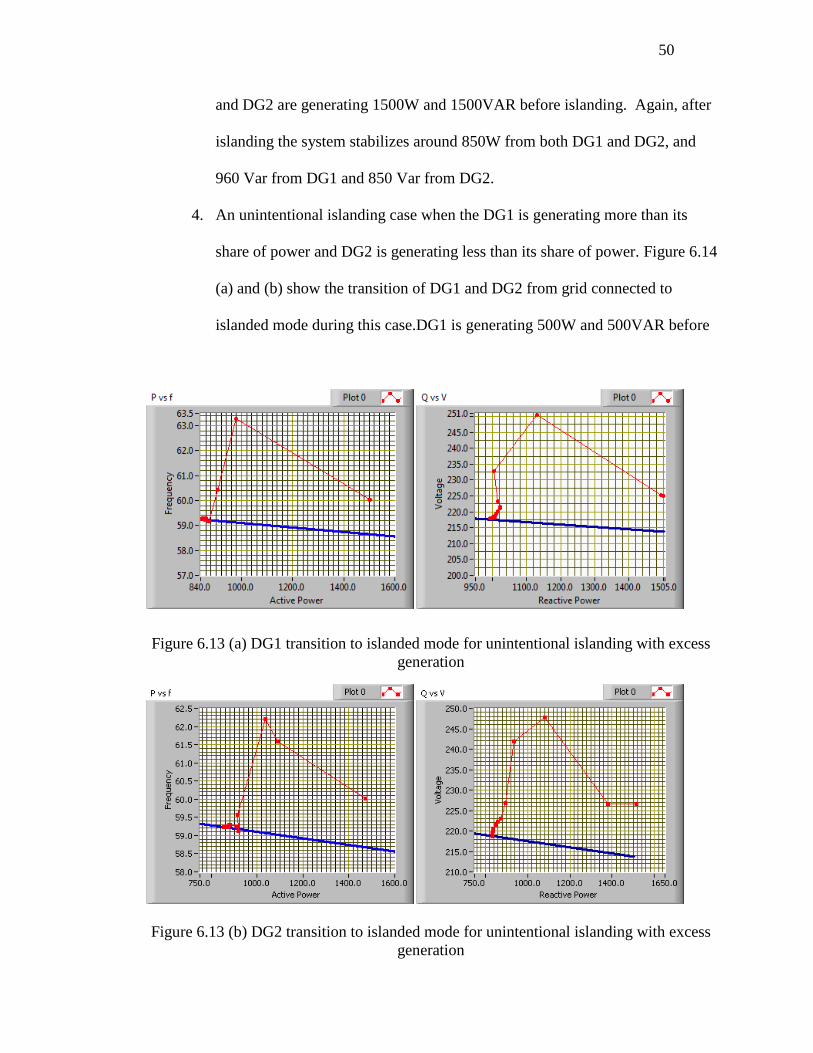
3. An unintentional islanding case when there is excess power in the system at
the instant of islanding. Figure 6.13 (a) and (b) show the transition of DG1
and DG2 from grid connected to islanded mode during this case. Both DG1
Figure 6.12 (a) DG1 transition to islanded mode for intentional islanding
Figure 6.12 (b) DG2 transition to islanded mode for intentional islanding
Page 63
50
and DG2 are generating 1500W and 1500VAR before islanding. Again, after
islanding the system stabilizes around 850W from both DG1 and DG2, and
960 Var from DG1 and 850 Var from DG2.
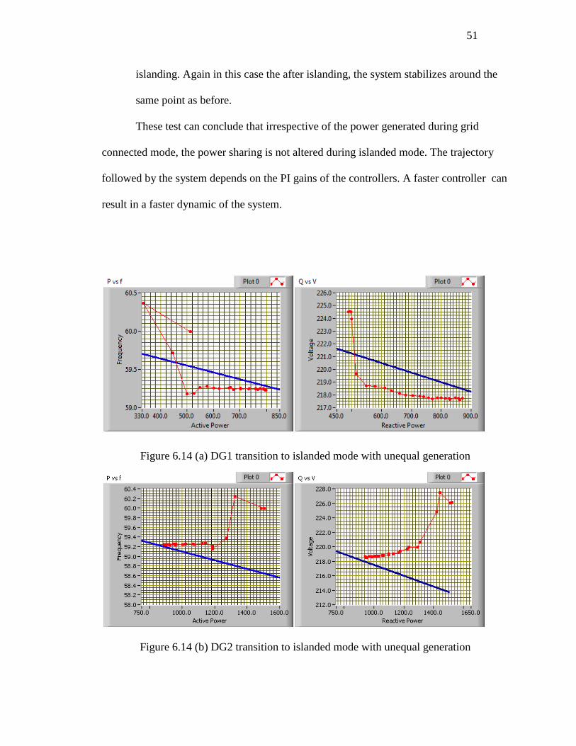
4. An unintentional islanding case when the DG1 is generating more than its
share of power and DG2 is generating less than its share of power. Figure 6.14
(a) and (b) show the transition of DG1 and DG2 from grid connected to
islanded mode during this case.DG1 is generating 500W and 500VAR before
Figure 6.13 (a) DG1 transition to islanded mode for unintentional islanding with excess
generation
Figure 6.13 (b) DG2 transition to islanded mode for unintentional islanding with excess
generation
Page 64
51
islanding. Again in this case the after islanding, the system stabilizes around the
same point as before.
These test can conclude that irrespective of the power generated during grid
connected mode, the power sharing is not altered during islanded mode. The trajectory
followed by the system depends on the PI gains of the controllers. A faster controller can
result in a faster dynamic of the system.
Figure 6.14 (a) DG1 transition to islanded mode with unequal generation
Figure 6.14 (b) DG2 transition to islanded mode with unequal generation
Page 65
52
6.2.5. Effect of Heavy Loads on System Performance. During islanded mode,
the system stability is maintained by the droop control. Droop control depends on active
and reactive power. Small changes in load can have a drastic impact on the voltage and
frequency. Figure 6.15 shows the system behavior during an extreme test when the
system load is changed from 0% to 100% of the rated load instantaneously. The
frequency and voltage drop below acceptable operating standards and will trigger any
protection equipment in the system but it can be observed that even during this extreme
case, the generators do not loose synchronism and the system is back to normal operating
conditions in 4 seconds. This is possible only because of the inertia based synchronous
machines in the system.
During normal operation of a microgrid system, the probability of a 4000W,
3000VAR load being turned on instantaneously in a 4000W, 3000VAR rated system is
very small. As explained in Section 6.1.2, the size of the transient depends on the size of
the load being added into the system. Thus this is the worst case transient. Since the
system is able to recover from the worst case transient, the system can be considered
stable for all transients. In reality the protection equipment would trip but in the
laboratory setup since there is no protection equipment the test was conducted.
Page 66
53
(a) Voltage at buses 1(V1), 2(V2) and 3(Vgrid)
(b) System frequency as calculated from the speed of DG1
(c) Active power flows from DG1(P1), DG2(P2) and grid(Pgrid) and that into bus 2 (Ptie)
(d) Reactive power flows from DG1(Q1), DG2(Q2) and grid(Qgrid) and that into bus 2 (Qtie)
Figure 6.15 System behavior when load is changed from 0% to 100% of rated load
0 20 40 60 80 100 120 140 160 180
50
100
150
200
Time(s)
Voltage(V
)
Vgrid
V1
V2
0 20 40 60 80 100 120 140 160 18045
50
55
60
Time(s)
Fre
quency(H
z)
0 20 40 60 80 100 120 140 160 180
0
500
1000
1500
2000
Time(s)
Active P
ow
er(
Watt
s)
Pgrid
P1
P2
Ptie
0 20 40 60 80 100 120 140 160 180
0
500
1000
1500
2000
Time(s)
Reactive P
ow
er(
VA
R)
Qgrid
Q1
Q2
Qtie
Page 67
54
7. CONCLUSION AND FUTURE WORK
A laboratory test bench is created for testing microgrid operation and control
schemes. A control scheme based on constant power mode and droop modes has been
proposed for the operation of the microgrid. It has been demonstrated that the loads in the
microgrid are served with nominal voltage and frequency with or without grid support
while ensuring that the generating units are stable and share the load. Operating
procedures for startup, unintentional islanding and intentional islanding have been
proposed and demonstrated. The microgrid has been tested with series and parallel
configurations, varied line lengths, and different droop settings. The impact of heavy
loads suddenly being turned on has been studied and it is proven that the system will
remain stable at all times.
In the future, the laboratory setting may be augmented with electronic loads and
inverter based DGs. Battery banks can be connected to the system to help during large
transients. There are various parameters involved in the control strategy such as droop
percentage, no-load frequency and voltage which can be modified to suit the system
requirements. Economic models can be incorporated into the selection of these
parameters. Protection issues can be studied and suitable protection schemes can be
incorporated into the microgrid.
Page 68
55
APPENDIX A
LABORATORY EQUIPMENT
Page 69
56
Figure A.1 Synchronous machine
Figure A.2 DC machine (Prime-mover)
Page 70
57
Figure A.3 DC machine drive
Figure A.4 Programmable Power Supply
Figure A.5 Protection for field power supply
Page 71
58
Figure A.6 Induction Machine – I Load
Figure A.7 Induction Machine – II Load
Page 72
59
Figure A.8 Resistive load banks
Figure A.9 Synchronization lamps
Page 73
60
APPENDIX B
LABORATORY WIRING DIAGRAMS
Page 74
61
Figure B.1 Connection panel
3 phase wattmeter – 1
3 phase wattmeter – 2
Syn. Machine contactor
Grid supply switch
Grid
conn.
Tie
line
conn.
Field
supply
conn.
Page 75
62
Figure B.2 DG1 wiring diagram
Syn. Machine
To local
load
To tie line From grid
PC
C
Fro
m f
ield
pow
er s
up
ply
DG
1 C
ab
le
Page 76
63
Figure B.3 DG2 wiring diagram
Syn. Machine
To local
load
To tie line
Fro
m f
ield
pow
er s
up
ply
Page 77
64
BIBLIOGRAPHY
[1] D. Moskovitz, “Profits and progress through distributed resources,” Regulatory
Assistance Project, Tech. Rep., Feb. 2010.
[2] P. Dondi, D. Boyoumi, C. Haederli, D. Julian, M. Suter, “Network Integration of
Distributed Power Generation,” J. Power Systems, vol. 106, pp. 1–9, 2002.
[3] P. Piagi, R.H. Lasseter, “Autonomous Control of Microgrids,” IEEE PES Meeting,
2006.
[4] IEEE Standards Coordination Committee 21, “IEEE Guide for Design, Operation,
and Integration of Distributed Resource Island Systems with Electric Power
Systems,” 2011.
[5] J. A. P. Lopes, C. L. Moreira, and A. G. Madureira, “Defining Control Strategies for
MicroGrids Islanded Operation,” IEEE Transactions on Power Systems, vol. 21, no.
2, pp. 916–924, May 2006.
[6] In-Su Bae and Jin-O Kim, “Reliability Evaluation of Customers in a Microgrid,”
IEEE Transactions on Power Systems, vol. 23, no. 3, pp. 1416–1422, Aug. 2008.
[7] R. Martinez-Cid and E. O’Neill-Carrillo, “Sustainable microgrids for isolated
systems,” IEEE PES Transmission and Distribution Conference and Exposition, pp.
1 –7. 2010.
[8] C. Marnay, F. J. Robio, and A. S. Siddiqui, “Shape of the microgrid,” IEEE Power
Engineering Society Winter Meeting, vol. 1, pp. 150 –153, 2001.
[9] A. Llaria, O. Curea, J. Jimenez, H. Camblong, “Survey on microgrids: Unplanned
islanding and related inverter control,” Intl. J. Renewable Energy, vol. 36, pp. 2052–
2061, 2011.
[10] N. D. Hatziargyriou, A. G. Anastasiadis, J. Vasiljevska, and A. G. Tsikalakis,
“Quantification of economic, environmental and operational benefits of Microgrids,”
in IEEE Bucharest PowerTech, pp. 1 –8, 2009.
[11] P. Barker, D. Herman, “Technical And Economic Feasibility of Microgrid-Based
Power Systems,” Seventh EPRI Distributed Resources Conference and Exhibition,
Mar. 2002.
[12] “Microgrids key to the smart grids evolution,” Power Engineering International,
vol. 18, no. 4, 2010.
[13]G. Venkataramanan and C. Marnay, “A larger role for microgrids,” IEEE Power and
Energy Magazine, vol. 6, no. 3, pp. 78–82, May 2008.
Page 78
65
[14] D. Pudjianto and G. Strbac, “Large Scale Integration of Microgeneration to Low
Voltage Grids, Work Package G: Regulatory regimes for supporting development of
micro-grids,” Prepared for the European Commission under contract # ENK5-CT-
2002-00610.
[15] D. E. King, “Electric Power Microgrids: Opportunities and Challenges for an
Emerging Distributed Energy Architecture,” Carnegie Melon University, Pittsburg,
2006.
[16] M. A. Pedrasa and T. Spooner, “A survey of techniques used to control microgrid
generation and storage during island operation,” in Australian Universities Power
Engineering Conf, 2006.
[17] M. Bollen, J. Zhong, and Y. Lin, “Performance indices and objectives for
microgrids,” in 20th International Conference and Exhibition on Electricity
Distribution-Part 1, pp. 1–4, 2009.
[18] F. A. Viawan and D. Karlsson, “Voltage and Reactive Power Control in Systems
With Synchronous Machine-Based Distributed Generation,” IEEE Transactions on
Power Delivery, vol. 23, no. 2, pp. 1079–1087, Apr. 2008.
[19] C. Cho, J. Jeon, J. Kim, S. Kwon, K. Park, and S. Kim, “Active Synchronizing
Control of a Microgrid,” IEEE Transactions on Power Electronics, no. 99, pp. 1–1,
2011.
[20] D. G. Shendell, R. Prill, W. J. Fisk, M. G. Apte, D. Blake, and D. Faulkner,
“Associations between classroom CO2 concentrations and student attendance in
Washington and Idaho,” Indoor Air, vol. 14, no. 5, pp. 333–341, 2004.
[21] R. H. Lasseter, “MicroGrids,” in Power Engineering Society Winter Meeting, vol. 1,
pp. 305–308, 2008.
[22] W. Yao, M. Chen, J. Matas, J. M. Guerrero, and Z.-M. Qian, “Design and Analysis
of the Droop Control Method for Parallel Inverters Considering the Impact of the
Complex Impedance on the Power Sharing,” IEEE Transactions on Industrial
Electronics, vol. 58, no. 2, pp. 576–588, Feb. 2011.
[23] T. L. Vandoorn, B. Meersman, J. D. M. De Kooning, and L. Vandevelde, “Directly-
Coupled Synchronous Generators With Converter Behavior in Islanded Microgrids,”
IEEE Transactions on Power Systems, 2012.
[24] E. T. Andrade, P. E. M. J. Ribeiro, J. O. P. Pinto, C.-L. Chen, J.-S. Lai, and N. Kees,
“A novel power calculation method for droop-control microgrid systems,” in
Twenty-Seventh Annual IEEE Applied Power Electronics Conference and Exposition
(APEC), pp. 2254 –2258, 2012.
Page 79
66
[25] F. Pilo, G. Pisano, and G. G. Soma, “Neural implementation of microgrid central
controllers,” in Industrial Informatics, 2007 5th IEEE International Conference on,
2007, vol. 2, pp. 1177–1182.
[26] A. L. Dimeas and N. D. Hatziargyriou, “Operation of a Multiagent System for
Microgrid Control,” IEEE Transactions on Power Systems, vol. 20, no. 3, pp. 1447–
1455, Aug. 2005.
[27] A. G. Tsikalakis and N. D. Hatziargyriou, “Centralized control for optimizing
microgrids operation,” IEEE Power and Energy Society General Meeting, pp. 1 –8,
2007.
[28] A. A. Zaidi and F. Kupzog, “Microgrid automation-a self-configuring approach,” in
IEEE International Multitopic Conference, pp. 565–570, 2007.
[29] S.-J. Ahn, J.-W. Park, I.-Y. Chung, S.-I. Moon, S.-H. Kang, and S.-R. Nam, “Power-
Sharing Method of Multiple Distributed Generators Considering Control Modes and
Configurations of a Microgrid,” IEEE Transactions on Power Delivery, vol. 25, no.
3, pp. 2007–2016, Jul. 2010.
[30] J. Jimeno, J. Anduaga, J. Oyarzabal, and A. G. de Muro, “Architecture of a
microgrid energy management system,” European Transactions on Electrical Power,
vol. 21, no. 2, pp. 1142–1158, 2011.
[31] H. J. Laaksonen, “Protection Principles for Future Microgrids,” IEEE Transactions
on Power Electronics, vol. 25, no. 12, pp. 2910–2918, Dec. 2010.
Page 80
67
VITA
Shyam Naren Bhaskara obtained his Bachelor of Technology degree in Electrical
and Electronics Engineering from Jawaharlal Nehru Technological University,
Hyderabad, India in May 2010. He received his Master of Science degree in Electrical
Engineering from Missouri University of Science and Technology in Aug 2012. His
research interests include power system operation and control, microgrids, and smart
grids.