Control and Optimization ofSupply Chain Networks

B. Erik Ydstie Duncan Coffey Mark ReadCarnegie Mellon Dow Chemicals Elkem Metals

AIM : Formulate supply chain problem as a network (electrical circuit) and see what inferences we can draw.

GOAL: Self Optimizing Enterprise

“..supply chain is a network of organizations involved through upstream and downstream linkages in different products and processes.”

Christopher, 1998

Outline:

1. Motivating Example: Silicon production2.The Supply Chain as a Process Network3.The Self Optimizing Enterprise4.Decentralized SCM main results5.Centralized SCM (Perea-Grossman)6. Industrial Case study # 2: Glass manufacture 7.Conclusions

Hydro/FossilPower

Quartzite Coal Wood Logs Limestone/sandElectrodes

Pre-treatment/Screen/Weigh/Mix

Rx 1 Rx 2 … Rx N

Refining Casting ChemicalPrimary Al

Secondary Al

CrushScreen

Raw material and Power Suppliers

Grind

Chemical Aluminum and Construction Industry

Flui

d Be

d

Dis

tilla

tion

Me2SiCl2 +++

SiliconesMotor oils

Fillers

90%

Flui

d/Fi

xed

Bed

10%

MeClCu

HCl

Siemen’sProcessWafering

Oxidation

SiCl3

Si WafersElectronics

Photovolatics

Fumed SilicaZeolytesCatalysts

Silicon for Chemicals and Electronics

Melting/blending

Silicon for primary and secondary Aluminum

Aluminum ++

Ingot castingExtrusionRollingCasting

Al platesContainers

Transportation

SiO2+C+O2=Si+SiO2(a)+CO2

1. From Si Manufacture to Finished Products

MicrroSilica

Electronics $3 Aluminum $1-2 Silicone

Memory Chips $40 Airplanes $12 Motor-oilsProcessors $60 Cars (Audi 6,++) Silicone fillersPhotoVoltaics $20 Trains +++++ Beverage cans

Profiles $7(windows, siding)

1ppb 7% Six-Oy-Hz

Silicon Demand 1,016,000 Mt (2001)

42,000 MT Si-eq 401,000 MT Si-eq 573,000 MT Si-eq

Construction, transportation, consumer goodsExchange rate, production in China, EU regulations

Silicon by Market Sectors

• Clean, Renewable Energy from the SUN• Silicon: 14-16% Efficiency• 0.1 kWp per m2

• 100 kWp per ton Silicon• Government Incentives in

EU, Japan and US

Current world wide SG-Si market ~$30M

Financial Outlook: Silicon for PhotoVoltaics

On gridCentralized

On gridDecentralized

Off GridCentralized

Off gridDecentralized

Market Outlook Silicon for PhotoVoltaics

050

100150200250300350400450

1990

1993

1996

1997

1998

1999

2000

2001

2002

2003

MWpEG-Scrap

R&D Programs: ELKEMSGSBayer/DegussaDow CorningAstropowerSHARPScanWanfer++

12 % Growth

slowing

25-30 % Growth

accelerating

99%+ Silicon based

KPMG 1999: Economies of Scale and Better Production facilities can reduce Solar electricity generating cost by a factor of 3

The Supply Chain for EG-Si and SG-Si

Cryst Wafers Etch.TCS Dist CVDSiO2 Red. Silgrain

Metallurgical Si - Silgrain 99.5% Electronic Grade Si 1ppb 12,000 tons/year

Solar CellsWafersRemelt/Cryst

Solar Grade Si 1 ppm

Scrap Silicon - tops/tails/rejects 2000 tons/year

Elkem, … BayerMitsubushiASiMI,..

DegussaSharpAMDIntel,…

CrystalloxScanwaferSharp,…

AstropowerSharp, ShellBP, Kyocera….

DegussaKyoceraNEC,..

Missing link

$1 /kg $3 /kg $40-60/kg

$5-20 /kg

42,000 tons/year

2,500 tons/year

Value added = $2

2. Process Networks: A Brief Review.Program: Establish an iso-morphism between process systems and network theory.

Electricity

Coal

Quartzite

Electronics

1. topology2. transportation3. shipping/receiving4. manufacture5. storage6. forecasting7. performance evaluation

Background: Circuit AnalysisMeixner (Irreversible thermo.) 1960Perelson (Biology) 1970Alonso Coffey Ydstie (control, stability,..) 1997Hangos, Cameron, Perkins (modeling) 1999Gilles (modeling) 1998+++

All flow is caused by driving force (potential)

Aims: PDE’s replaced with ODE’sfocus on topologystability and controloptimizationdistribution of computationsease of modelingmodular software designvisualizationflows and ext. var. are additive++++

P

S S

S S S

S

Al(1) Al(2) Chemical

Heat and off gas Micro SilicaPowerQuartziteCoal

Electrical PowerElectrical Power

Quartz (SiO2), Carbon (C)Quartz (SiO2), Carbon (C)SiO, COSiO, CO

Silicon (Si(l))Silicon (Si(l))

(1+a) SiO2 + SiC → (1-a) Si(l) + (1-2a) SiO(g) + CO(g)(1+a) SiO2 + SiC → (1-a) Si(l) + (1-2a) SiO(g) + CO(g)

SiO(g) + 2 C → SiC + CO(g)

2a SiO → a SiO2 +a Si

SiO(g) + 2 C → SiC + CO(g)

2a SiO → a SiO2 +a Si

A A ASilicon Aluminum alloys

CastingRollingExtrusion,

Engine partsProfilesSheets++

Process ControlStabilization

Real Time Optimization

Supply Chain Management

S

P

TR

T

Assets A = {v,c,z}Activities (flow of assets) F = {f,z}

v – extensive variable (amount /charge)c – intensive variable (value/voltage)f – rate of flow of an extensive variable (flow rate/current)z – characterization (SKU, composition, etc.)

G=(P,S,T,R,H)

P – production/manufactureS – storageT – terminalsR – routingH – transportation

H

Activity

rate [units/time] , value generation [value/unit]

Σ fi=0

Material balanceKirchoff current law

S

dvdt = f

StorageCapacitor

InductorDiode+

Routing point Storage Activity and terminals

Rf=w

FourierFickNewtonOhm’s Laws

Constitutive equations

Conservation Laws Potential Flow

Activity Based Analysis – Value added as driving force

Each activity adds value (positive or negative)

Cos

t/Val

ue p

er u

nit $

Raw MaterialPurchase

Move and storeraw material

Produce Move and storefinished products

Sell and shipFinished products Activity

Purchase price

Added value w=cn-cn-1

Sale price

S

PH

Direction of flow: From low to higher value is positivefrom high to low value is negative

Net (internal) activity Cost:

Cost (internal) of operations:

Net rate of profit [$/sec]:

Circular activity does not add value: (Kirchoff’s voltage law)

Cost/dissipation: (2nd law of thermo)

Financial Implications:

-P plays the role of “energy”

G

f w

N-port

Diathermal

AdiabaticSem

i-per

mab

le T Sµ

N

-p

V

Thermodynamics Networks

Conservation laws Convex Energy function U(N,S.V)

Intensive variables via Legendre transform

Kirchoff’s Current LawKirchoff’s Voltage Law

U

f

Network builds itself into an energy minimizer!!!

G

c1 c2

Supplied energy:

Dissipation:

0 0.1 0.2 0.3 0.4-0.2

-0.1

0

0.1

0.2

0.3

0.4

0.5

T-C

r=10w=1

f

w

One port example

G

c1 c2

Supplied energy:

Dissipation:

0 0.1 0.2 0.3 0.4-0.2

-0.1

0

0.1

0.2

0.3

0.4

0.5

T-C

One port example

Generalizes to RLC and we get stability

3. The Self-Optimizing Enterprise

• One-ports (terminals, storage, production, activities, routers, +++)• Conservation of assets (KCL)• Circular activity does not add value (KVL)

f1 f2 f3 f4 f5 f6 f7

Distributed Enterprise

1. The enterprise consists of a (large) number of nodes.2. Connected with the “world” at terminal points (boundary conditions).3. Flows are the result of potential at the terminal.

Tellegen’s Theorem – a Topological Result

“Building the Self-Optimizing Enterprise”

• One-ports (terminals, storage, production, activities, routers, +++)• Conservation of assets (KCL)• Circular activity does not add value (KVL)

Distributed EnterpriseDistributed Enterprise (a)

Flows and costs are orthogonal

Enterprises (a) and (b) have same topology.Same enterprise in different states

Tellegen’s Theorem – a Topological Result

“Building the Self-Optimizing Enterprise”

• One-ports (terminals, storage, production, activities, routers, +++)• Conservation of assets (KCL)• Circular activity does not add value (KVL)

Distributed EnterpriseDistributed Enterprise (a)

Filtered lows and costs are orthogonal

Network operator – filter, forecast, Fourier transform, expectation,..

1. Existence and uniqueness of solutions if the routing policies are positive (negative).

2. Added value (cost) is stationary.3. Added value (cost) is maximized (minimized) if the routing

policies are negative.

Assumptions: Assets are conservedCircular activity does not add value

4. Decentralized SCM: Optimality Results

∆f

∆w ∆f

∆w

The activity cost is not positive

f

w

f

f

w

w(A) (B)

(C)

Capacity Constraint

f

w(D)

Discount for large volumes

Neutral costNegativemonotonicity

Positivemonotonicity

4. Decentralized SCM: Optimality Results

1. Existence and uniqueness of solutions if the routing policies are positive (negative).

2. Cost is stationary3. Passivity can be used to investigate stability..

Assumptions: Assets are conservedCircular activity does not add value

Load Balancing - Parallel Activities

1

2

wCooperative -stabilize Competitive - unstable

0 1 0 1

Competitive markets give narrow margins and pressure toreduce cost to stay in business.

Develop new products and new processes.Dominate market.Seek (cost) advantage (geographical, sourcing,…..

Cost Balancing - Serial Activities

1 2

w1

“Cooperative”

0 f

r1f1=w1 r2f2=w2

w2

w=w1+w2f=f1=f2

“Fair” transfer price::

w

Advantageous not to share information

(may be too limited)

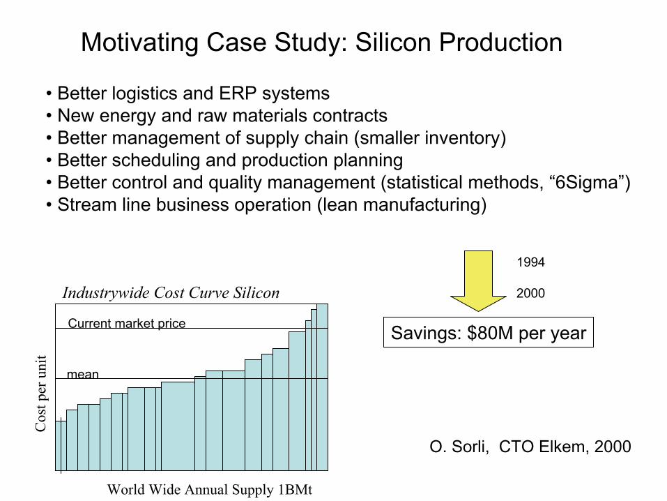
Industrywide Cost Curve Silicon

Cos

t per

uni

t

World Wide Annual Supply 1BMt

Savings: $80M per year

• Better logistics and ERP systems• New energy and raw materials contracts• Better management of supply chain (smaller inventory)• Better scheduling and production planning• Better control and quality management (statistical methods, “6Sigma”)• Stream line business operation (lean manufacturing)

mean

Current market price

Motivating Case Study: Silicon Production

O. Sorli, CTO Elkem, 2000

1994

2000

Batch HouseBatch Mix

Hot End Cold End Cutting/Packaging

I/O I/O I/O I/OI/O

PC/Workstation PC/Workstation PC/Workstation

PLC -LogicStochastic ControlKalman Filter

PLC -LogicStochastic ControlEHACPID/FFMachine VisionNonlinear Adaptive Combustion AirNonlinear Compensation for Air Pressure Control

Nonlinear EstimatorTweel control Machine Vision

Optimal CuttingMachine VisionPLC-Logic

Technical IT AlgorithmsCommunication

Activities InventoryFlows

InterfaceActuatorsSensors

Crown I

Melter II

Refiner IVWaist III Canal V

Industrial Case Study #2: Glass Production

Quality checkLaminatingPackagingDelivery(MB/BMW)

Replacement parts

Activity

Actuators/Sensors

VirtualActivity

Smart Measurements

Raw materialand energy inputs

Molten glassand energy outputs

Virtual inputs Virtual outputs

Real Process

Virtual Process

RealMeasurements

VirtualMeasurements

Sensor Module

Distributed Systems thatIntegrate Physics and Communication

Distributed system of process activities

Sensor, actuator control

Network of computers, databases and software for control and optimization (Technical IT)

raw materials Intermediates and products

Accounting and finance (Business IT) Man/Machine Interface

Sensor, actuator control Sensor, actuator control

Control moduleOptimization module6Sigma module*****

Activities

Interface

Software

Estimated savings $35M per year

PW1

C1

A/B/C

D/E/F

G/H/I

A/B/C

D/G/H/I

A/D/F/G/I

D/E/F

C/G/H/I

C/F/I

C/E/G

G/H/I

B/E/G

A/F/G

A/B/C

D/E/F

D/E/F

G/H/I

D/E/F/G/H/I

A/B/C/D/E

F/H/I

A/D/E

B/C/E

A/D/G

Plants & Warehouses

Distribution Centers

Retailers Customers

A/B/C/D/E/F/G/H/I

A/B/C/D/E/F

A/F/G

C/E/F/G/I

C/D/E/F/G/H/I

A/D/F/G/H/I

A/B/C/D/E/F/H/I

A/D/G

A/B/C/D/E

B/C/E/F/G/H/I

A/B/C/D/E/F/G/H/ID/E/F/G/H/I

D/E/F

A/C/D/E/F/G/H/I

PW3

PW2

DC1

`DC2

DC3

DC4

RT1

RT2

RT3

RT4

RT5

RT6

RT7

RT8

RT9

RT10

C2

C4

C3

C5

C6

C8

C10

C12

C13

C14

C15

C18

C19

C20

C7

C17

C9

C11

C16

B/E/G/H/I

PW1

C1

A/B/C

D/E/F

G/H/I

A/B/C

D/G/H/I

A/D/F/G/I

D/E/F

C/G/H/I

C/F/I

C/E/G

G/H/I

B/E/G

A/F/G

A/B/C

D/E/F

D/E/F

G/H/I

D/E/F/G/H/I

A/B/C/D/E

F/H/I

A/D/E

B/C/E

A/D/G

Plants & Warehouses

Distribution Centers

Retailers Customers

A/B/C/D/E/F/G/H/I

A/B/C/D/E/F

A/F/G

C/E/F/G/I

C/D/E/F/G/H/I

A/D/F/G/H/I

A/B/C/D/E/F/H/I

A/D/G

A/B/C/D/E

B/C/E/F/G/H/I

A/B/C/D/E/F/G/H/ID/E/F/G/H/I

D/E/F

A/C/D/E/F/G/H/I

PW3

PW2

DC1

`DC2

DC3

DC4

RT1

RT2

RT3

RT4

RT5

RT6

RT7

RT8

RT9

RT10

C2

C4

C3

C5

C6

C8

C10

C12

C13

C14

C15

C18

C19

C20

C7

C17

C9

C11

C16

B/E/G/H/I

Material Flow(A, B or C)Information Flow(Orders)

Distr. Center

Plant Warehouse

Retailer CustomerPlant

ukk’’

t

ykc

dkc

Ik’,Ok’k ykk’’yk’k

uk’k

upk’Raw materials

supplier

yk`k``

uk`k``

ukk’’, upk’: Inputsdkc: DisturbancesIk,Okk’’: Statesykk’’,yk’’c: Outputs

Ik,Okk’’ Ik’’,Okc

Material Flow(A, B or C)Information Flow(Orders)

Material Flow(A, B or C)Information Flow(Orders)

Distr. Center

Plant Warehouse

Retailer CustomerPlant

ukk’’

t

ykc

dkc

Ik’,Ok’k ykk’’yk’k

uk’k

upk’Raw materials

supplier

yk`k``

uk`k``

ukk’’, upk’: Inputsdkc: DisturbancesIk,Okk’’: Statesykk’’,yk’’c: Outputs

Ik,Okk’’ Ik’’,Okc

5. Centralized SCM using MPC(Perea-Grossmann-Ydstie, 2002)

Plant and order delaysDiscrete manufactureMaximize profit

Solve using MPC strategy

Case 1: Optimal Integrated

0

5000

10000

15000

20000

1 13 25 37 49 61 73Time

Inve

ntor

y at

DC

1

D1I D2A D2C D2D D2E D2F D2G D2H

Case 3: Optimal Scheduling

0

5000

10000

15000

20000

1 13 25 37 49 61 73Time

Inve

ntor

y at

DC

1

D2A D2C D2D D2E D2F D2G D2H D2I

Case 1: Optimal Integrated

0

5000

10000

15000

20000

1 13 25 37 49 61 73Time

Inve

ntor

y at

DC

1

D1I D2A D2C D2D D2E D2F D2G D2H

Case 3: Optimal Scheduling

0

5000

10000

15000

20000

1 13 25 37 49 61 73Time

Inve

ntor

y at

DC

1

D2A D2C D2D D2E D2F D2G D2H D2I

• Better balance of plant schedule and inventory levels in CSM. • Centralized planning needed when the delays are long.• Too short planning horizon T < 6 days gives myopic policy (plant shuts down).• Policy insensitve to planning horizon for T .> 12 days.

Edgar Perea-Lopez, Grossmann Ydstie 2002.

GAMS / XPRESS-MP to solve MILP. Discrete time elements = 2hr. Prediction horizon of 12 days (144 elements of 2 hr each). Weekly updates updates of the demand, MILP model with 1,296 binary, 85,898 continuous variables and 59,150 constraints.

Summary• Practical control systems are built up from the bottom using

distributed modules.• Decentralized control and decision making can be “optimal” (self

optimization).• Parallel distributed computing is a reality. Numerical methods and

software is needed to take advantage.• Cutting cost vs new product and process.• Margins converge and become smaller over time in a competitive

commodity market.• Large, “hybrid” dynamic system solved to optimality (mpc).• Large savings possible• But, there is no “silver bullet”. Broad spectrum of technologies

need to be integrated with the process and Business IT system.

Acknowledgements: B. Marshall ALCOA Technical Center PghO. Sorli ELKEM ASAT. Halmo ELKEM ASA/StatoilY. Jiao PPG Inc Pgh