HAL Id: tel-01761771 https://hal.archives-ouvertes.fr/tel-01761771 Submitted on 9 Apr 2018 HAL is a multi-disciplinary open access archive for the deposit and dissemination of sci- entific research documents, whether they are pub- lished or not. The documents may come from teaching and research institutions in France or abroad, or from public or private research centers. L’archive ouverte pluridisciplinaire HAL, est destinée au dépôt et à la diffusion de documents scientifiques de niveau recherche, publiés ou non, émanant des établissements d’enseignement et de recherche français ou étrangers, des laboratoires publics ou privés. Control of Hybrid Systems and Discrete-Event Systems Naly Rakoto-Ravalontsalama To cite this version: Naly Rakoto-Ravalontsalama. Control of Hybrid Systems and Discrete-Event Systems. Computer Science [cs]. IMT Atlantique, 2017. tel-01761771
Transcript
HAL Id: tel-01761771https://hal.archives-ouvertes.fr/tel-01761771
Submitted on 9 Apr 2018
HAL is a multi-disciplinary open accessarchive for the deposit and dissemination of sci-entific research documents, whether they are pub-lished or not. The documents may come fromteaching and research institutions in France orabroad, or from public or private research centers.
L’archive ouverte pluridisciplinaire HAL, estdestinée au dépôt et à la diffusion de documentsscientifiques de niveau recherche, publiés ou non,émanant des établissements d’enseignement et derecherche français ou étrangers, des laboratoirespublics ou privés.
Control of Hybrid Systems and Discrete-Event SystemsNaly Rakoto-Ravalontsalama
To cite this version:Naly Rakoto-Ravalontsalama. Control of Hybrid Systems and Discrete-Event Systems. ComputerScience [cs]. IMT Atlantique, 2017. �tel-01761771�
Control of Hybrid Systems and Discrete-Event Systems
Commande de Systemes Hybrides et de Systemes a Evenements Discrets
Ecole Doctorale : STIMSpecialization: Automatic Control
Date of defense: 6 September 2017
EXAMINING COMMITTEE
Reviewers:
Didier Henrion Research Director, LAAS-CNRS ToulouseDaniel Liberzon Professor, University of Illinois at Urbana-Champaign, USAEric Niel Professor, INSA Lyon - Ampere
Examiners:
Alexandre Dolgui Professor, IMT Atlantique - LS2NClaude Jard Professor, University of Nantes - LS2NStephane Lafortune Professor, University of Michigan, Ann Arbor, USAJean-Jacques Loiseau Research Director, CNRS - LS2N
• les rapporteurs : Didier Henrion, Daniel Liberzon et Eric Niel.
• les examinateurs : Alexandre Dolgui, Claude Jard, Stephane Lafortune et Jean-JacquesLoiseau.
• mes Doctorants: Santi, Jose-Luis, Eduardo et German.
• ma famille : Pascale, Alice et Camille, et ma mere, Emilienne
Enfin, cette These d’HDR est dediee a la memoire de mon pere, Prof. Dr. Georges Rakoto-Ravalontsalama (1937-2011).
5
NR HDR 6
Introduction
The HDR (Habilitation a Diriger des Recherches) is a French Degree that you get some years afterthe PhD. It allows the candidate to apply for some University Professor positions and/or to applyfor a Research Director position at CNRS. Instead of explaining it in details, the selection phasesprocess after an HDR is summarized with a Petri Net model in Figure 1.
n
selec−n
qualification (CNU)
HDR
Professor
univ−1 univ−2 univ−nCNRS
Research Director
selec−1selection
2
Figure 1: Selection Phases after the HDR
After obtaining the HDR Thesis Degree, the candidate is allowed to apply for a Research Directorposition at CNRS, after a national selection. On the other hand, in order to apply for some Univer-sity Professor positions, the candidate should first apply for a National Qualifcation (CNU). Oncethis qualification obtained, the candidate can then apply to some University Professor positions,with a selection specific to each university.This HDR Thesis is an extended abstract of my research work from my PhD Thesis defense in 1993until now. This report is organized as follows.
• Chapter 1 is a Curriculum Vitae
• Chapter 2 presents the Analysis and Control of Hybrid and Switched System
• Chapter 3 is devoted to Supervisory Control of Discrete-Event Systems
• Chapter 4 gives the Conclusion and Future Work
7
NR HDR 8
Chapter 1
Curriculum Vitae
1.1 Personal Data
Born on February 19, 1965; Married and has 2 daughters (19 and 15 years old, resp.)Citizenship: French.
A. Affiliation
- Dept. of Automation, Production and Computer Science (DAPI)IMT Atlantique (ex-Mines Nantes) Phone: +33 (0)2 5185 83064 Rue Alfred Kastler Fax: +33 (0)2 5185 834944307 Nantes Cedex 03 e-mail: [email protected]
France web: www.imt-atlantique.fr
- Also member of LS2N Laboratory, Nantes (UMR CNRS 6004) in the PSI Research Groupwww.ls2n.fr
B. Education
1993 Ph.D. in Automatic Control (Tres Honorable) LAAS-CNRS and University of Toulouse, France1989 M.Sc. [DEA] in Automatic Control (A. Bien) LAAS-CNRS and University of Toulouse, France1987-88 Licence + Maıtrise EEA (Assez Bien) University of Toulouse, France1985 DEUG A Physique-Chimie (Bien) University of Toulouse, France1983 National Service Tananarive, Madagascar1982 Baccalaureat serie C (Assez Bien) Tananarive, Madagascar
1.2 Teaching Activities
A. Teaching
I am teaching regularly a yearly normal service i.e. 192 h eq TD since I arrived at Ecole desMines in September 1994. The subject and the students have a bit evolved since 1994. Herebelow is a summary of the courses that I gave during the Academic year 2015-2016. What is newcompared to the beginning in 1994 are the courses given in the 2 Master of Science programs MOST(Management and Optimization in Supply Chain and Transport) and PM3E (Project Managementfor Environmental, and Energy Engineering). These 2 programs are offered entirely in English.
9
NR HDR 10
Promo Course CM PC TD TP-MP PFE Resp Lang.A1 Automatique 10h 10h 10h Fr.A2 Optim. 10h 5h Fr.A2 AII SED 10h 5h 5h Fr.A3 AII SysHybrides 7.5h 7.5h Fr.MSc. PM3E Control 7.5h 7.5h Eng.MSc. MOST Simulation 5h 5h 5h Eng.MSc. MOST Resp. MSc+UV 90h Eng.A3 PFE superv. 36h Fr.Masters PFE superv. 36h Eng.
B. Responsabilities (Option AII, Auto-Prod, MSc MLPS, MSc MOST)
I had and am having the following administrative responsabilities at Mines Nantes:
• 1997-2000: Last Year’s Option AII (Automatique et Informatique Industrielle)
• 2001-2004: First and Second Year: Control and Industrial Eng. courses at DAP
• 2006-2012: MSc. MLPS (Management of Logistic and Production Systems)
• 2012-present: MSc. MOST (Management and Optimization of Supply Chains and Transport)
C. Courses given abroad
• May 2008: Univ. of Cagliari (Italy): Control of Hybrid Systems (10h) Erasmus
• Apr. 2009: Univ. Tec. Bolivar UTB, Cartagena (Colombia): Tutorial on DES (15h)
• May 2014: Univ. Tec. Bolivar UTB, Cartagena (Colombia): Intro. to DES (15h)
• Dec 2015: ITB Bandung (Indonesia): Simulation with Petri Nets (10h) Erasmus
• Apr. 2017: Univ. of Liverpool (UK): Course 1 (10h) Erasmus
• May 2017: ITB Bandung (Indonesia): Simulation with Petri Nets (10h) Erasmus
1.3 Research Activities
My main topics of research are the following:
1. Analysis and control of hybrid and switched systems
2. Supervisory control of discrete-event systems
These will be detailed in Chapter 2 and Chapter 3, respectively. The following other topics ofresearch will not be presented. However, the corresponding papers can be found in the CompleteList of Publications.
• Resource Allocation
• Holonic Systems
• Inventory Control
NR HDR 11
1.4 Supervision of Students: PhD, MSc.
A. PhD Students:
• Santi Esteva, PhD defended in Girona in March 2003.-Modelling, Control and Supervision for a Class of Hybrid Systems- PhD Committee: J. Aguilar-Martin, J.L. de la Rosa, J. Colomer, J.C. Hennet, E. Garcia,J. Melendez, V. Puig, N. Rakoto, G. Roux- Supervision: J.L. de la Rosa (50 %), N. Rakoto (50 %)- Publications: 1 conference paper- Current activity: Associate Professor at University of Girona, Spain.
• Jose-Luis Villa, PhD defended in Nantes in February 2004.-Modelisation et commande de systemes hybrides : L’approche MLD- PhD Committee: M. Morari, K.E. Arzen, M. Duque, A. Gauthier, J.J. Loiseau, N. Rakoto- Supervision: M. Duque (40 %), A. Gauthier (10 %), N. Rakoto (40 %), J.J. Loiseau (10 %)- Publications: 1 book chapter, 12 conference papers- Current activity: Profesor Titular at Universidad Tecnologica Bolivar, Cartagena, Colombia.
• Eduardo Mojica, PhD defended in Nantes in September 2009.-A polynomial approach for analysis and optimal control of switched nonlinear systems- PhD Committee: P. Caines, D. Henrion, A. Gauthier, J.J. Loiseau, N. Quijano,P. Riedinger, N. Rakoto- Supervision: M. Quijano (40 %), A. Gauthier (10 %), N. Rakoto (40 %), J.J. Loiseau (10%)- Publications: 2 journal papers, 6 conference papers- Current activity: Associate Professor at Universidad Nacional, Bogota, Colombia.
• German Obando, PhD defended in Nantes in October 2015.-Distributed methods for resource allocation: A passivity-based approach- PhD Committee: C. Ocampo-Martinez, H. Gueguen, A. Dolgui, A. Gauthier,J.J. Loiseau, N. Quijano, N. Rakoto- Supervision: M. Quijano (40 %), A. Gauthier (10 %), N. Rakoto (40 %), J.J. Loiseau (10%)- Publications: 1 journal paper, 2 conference papers- Current activity: PostDoc at Universidad de los Andes, Bogota, Colombia.
B. MSc Students:
• 2017: Nawapol Yamclee (IMTA / MSc. PM3E) – Control of Smart Grids
• 2017: Dina Lavender (IMTA / MSc. MOST) – Simulation with Stochastic Petri Nets
• 2010: Amadou Sagna (ECN / Master AIA) – Model Predictive Control
• 1994: Jean-Sebastien Besse (INSA Toulouse) – G2 Expert System
C. Member of Ph.D. Thesis Committees (other than my PhD Students)
- Ph.D. examiner of D. Fragkoulis, LAAS-CNRS, Univ. of Toulouse, France (Nov. 2008)Detection et localisation des defauts provenant des capteurs et des actionneurs :
application sur un systeme non lineaire.
NR HDR 12
- Ph.D. examiner of Aimed Mokhtari, LAAS-CNRS, Univ. of Toulouse, France (Sep. 2007)Diagnostic de systemes hybrides : developpement d’une methode associant la detection par
classification et la simulation dynamique.
- Ph.D. examiner of Hector Hernandez de Leon, LAAS-CNRS, Univ. of Toulouse, France (Sep. 2006)Supervision et diagnostic des procedes de production d’eau potable.
- Ph.D. examiner of Flavio Neves-Junior, LAAS-CNRS, Univ. of Toulouse, France (Nov. 1998)Supervision et commande des phases transitoires des processus industriels : application a unecolonne de distillation.
D. Short Research Visits
- May-June 2004: McGill University, Montreal, Canada. Host: Prof. Peter E. Caines (2 months)- Sep. 2013: University of Michigan, Ann Arbor, MI, USA. Host: Prof. Stephane Lafortune (1 month)
E. Invited Plenary Talks
- Invited Plenary Talk, Analysis and Control of Hybrid and Switched Systems, ColombianControl Conf., Cartagena, Colombia, April 2009.
F. Member of Conference International Program Committees
- IFAC Conf. on Analysis and Design of Hybrid Systems (ADHS 2006), Alghero, Italy, June 2006.- IEEE Conf. on Emerging Technologies and Factory Automation (ETFA 2001) Antibes, FR, 2001- Int. Conf. on Automation of Mixed Processes: (ADPM 1998), Reims, France, March 1998.
G. Member of Conference Organizing Committees
- 7th Workshop on Service Orientation in Holonic and Multi-Agent Manufacturing(SOHOMA 2017) Nantes, France, 2017.- IFAC Conf. on Analysis and Design of Hybrid Systems (ADHS 2003), St. Malo, France, 2003.- Conf. Int. Francophone en Automatique (CIFA 2002), Nantes, France, July 2002.- Int. Conf. on Automation of Mixed Processes (ADPM 2000), Dortmund, Germany, Sep. 2000.
1.5 Funded and Submitted Projects
• Co-Principal Investigator (with Andi Cakravastia, ITB), LOG-FLOW, PHCNUSANTARA France Indonesia, Project N. 39069ZJ, 2017, Accepted on 31 May 2017.
• Participant, ”Industrial Validation of Hybrid Systems”, France and Colombia ECOS NordProject N.C07M03, A. Gauthier and J.J. Loiseau PIs, Jan. 2007 to Dec. 2009 (3 years)Euro 12,000.
• Participant, French ”Contrat Etat-Region” 2000-2006, CER STIC 9 / N.18036,J.J. Loiseau PI, Euro 182,940 (US$ 182,940).
• Co-Principal Investigator (with Ph. Chevrel), Modeling and Simulation of ESP Program,Peugeot-Citroen PSA France, Sep. 2000 - Jan 2001, FF 20,000 (US$ 3,000).
• Co-Principal Investigator (with J. Aguilar-Martin), Control and Supervision of a DistillationProcess, Conseil Regional Midi-Pyrenees, France, 1994-1995, FF 200,000 (US$ 30,000).
• Participant, European Esprit Project IPCES (Intelligent Process Control by means ofExpert Systems), J. Aguilar-Martin PI, 1989-1992, Euro 500,000 (US$ 500,000).
NR HDR 13
1.6 Organization of Invited Sessions
- Invited Session, Diagnosis and Prognosis of Discrete-Event Systems, 48th IEEE CDCShanghai, China, Dec 2009(jointly organized and chaired with Shigemasa Takai).
- Invited Session, Diagnosis of DES Systems, 1st IFAC DCDS 2007, Paris, France, June 2007(jointly organized and chaired with Shigemasa Takai).
- Invited Session, DES and Hybrid Systems, IEICE NOLTA 2006, Bologna, Italy, Sep. 2006(jointly organized and chaired with Shigemasa Takai).
- Invited Session, Supervisory Control, IFAC WODES, Reims, France, Sep. 2004(jointly organized and chaired with Toshimitsu Ushio).
- Invited Session, Hybrid Systems, IEEE ISIC 2001, Mexico City, Mexico, Sep. 2001(jointly organized and chaired with Michael Lemmon).
- Invited Session, Knowledge Based Systems, IEEE ISIC 1999, Cambridge, MA, USA, Sep. 1999(jointly organized and chaired with Karl-Erik Arzen).
- Workshop on G2 Expert System, LAAS-CNRS, Toulouse, France, Oct. 1995(jointly organized and chaired with Joseph Aguilar-Martin).
1.7 Complete List of Publications
A summary of the papers, classified per year, from 1994 to 2017, is given in the following table.
Conf. Book Chap. Book Ed. Journal Total
1994 2 2
1995 2 1 1 4
1996 1 1 2
1997 1 1
1998 2 2
1999 1 1
2000
2001 4 1 5
2002 1 1
2003 5 1 6
2004 6 6
2005 1 1
2006 3 3
2007 4 4
2008 2 2
2009 1 1
2010 1 1
2011
2012 1 1
2013 2 2
2014 4 1 5
2015 2 1 3
2016 4 4
2017 1+3* 1* 1+4*
Table 1.2: Number of published papers per year (as of 30 June 2017) – where (*) means submitted
NR HDR 14
Complete List of Publications
[] Book Edition
[B.1] Supervision de processus a l’aide du systeme expert G2, N. Rakoto-Ravalontsalama and J.Aguilar-Martin (Eds.), Hermes Ed. Paris, Oct. 1995, ISBN 2-86601-499-5.
[Proceedings of Workshop on G2 Expert System, LAAS-CNRS Toulouse, France, Oct. 1995][Includes 4 papers in English and 6 papers in French]
International Refereed Journals
[J.sub1] F. Torres, C. Garcia-Diaz and N. Rakoto-Ravalontsalama. ”Evolutionary Dynamics ofTwo-actor VMI-driven Supply Chains”, Submitted, Dec. 2016.
[J.9] G. Obando, N. Quijano, and N. Rakoto-Ravalontsalama. ”A Center-Free Approach forResource Allocation with Lower Bounds”, International Journal of Control, 2016. DOI:10.1080/00207179.2016.1225167.
[J.8] C. Indriago, O. Cardin, N. Rakoto-Ravalontsalama, P. Castagna, E. Chacon. ”H2CM: Aholonic architecture for flexible hybrid control systems”’, Computers in Industry, Elsevier, 77(2016) pp. 15–28.
[J.7] C. Indriago, O. Cardin, O. Morineau, N. Rakoto-Ravalontsalama, P. Castagna, E. Chacon.”Performance evaluation of holonic control of a switch arrival system”’, Concurrent Engineer-ing: Research and Applications, SAGE, 2016, DOI: 10.1177/1063293X16643568.
[J.6] C. Indriago, O. Cardin, O. Bellenguez-Morineau, N. Rakoto, P. Castagna, E. Chacon. ”Evalu-ation de l’application du paradigme holonique a un systeme de reservoirs”’, Journal Europeendes Systemes Automatises JESA, vol. 49 N.23, pp.325-347, 2016.
[J.5] E. Mojica, N. Quijano, and N. Rakoto-Ravalontsalama A polynomial approach for optimalcontrol of switched nonlinear systems, Int. Journal of Robust and Nonlinear Control, Wiley,2014, 24 (12), pp.1797-1808.
[J.4] E. Mojica, N. Quijano, N. Rakoto-Ravalontsalama, and A. Gauthier A polynomial approachfor stability analysis of switched systems, Systems and Control Letters 59 (2010) 98–104.
[J.3] N. Rakoto-Ravalontsalama, J. Aguilar-Martin, Knowledge-based modelling of a TV-tube man-ufacturing system, IFAC Journal of Control Engineering Practice, Jan. 1996, 4(1), pp. 117–123.
[J.2] P. Bourseau, K. Bousson, P. Dague, J.L. Dormoy, J.M. Evrard, F. Guerrin, L. Leyval, O.Lhomme, B. Lucas, A. Missier, J. Montmain, N. Piera, N. Rakoto-Ravalontsalama, J.P. Steyer,M. Tomasena, L. Trave-Massuyes, M. Vescovi, S. Xanthakis and B. Yannou, Qualitativereasoning: A survey of techniques and applications AICOM Journal, Sept-Dec. 1995, vol. 8,N. 3-4, pp. 119–192.
[J.1] N. Rakoto-Ravalontsalama, A Missier, and J.S. Kikkert, Qualitative operators and process en-gineer semantics of uncertainty. In B. Bouchon-Meunier, L. Valverde, and R.R. Yager (Eds.)
15
NR HDR 16
Lecture Notes in Computer Science N. 682, IPMU’92 - Advanced Methods in Artificial Intel-ligence, Springer Verlag 1992, pp. 284–293.
Book Chapters
[B.Ch.4] C. Indriago, O. Cardin, N. Rakoto, E. Chacon, P. Castagna, ”Application of holonicparadigm to hybrid processes: Case of a water treatment process”’ Chapter of the book ”Ser-vice Orientation in Holonic and Multi-agent Manufacturing”, Springer, 2015 ISBN 978-3-319-15159-5.
[B.Ch.3] J.L. Villa, M. Duque, A. Gauthier, and N. Rakoto-Ravalontsalama, Hybrid modeling ofpotable water treatment plant. In. Pumps, Electromechanical Devices and Systems Applied toUrban Water Management, Cabrera and Cabrera Jr. Eds., 2003 Swets and Zeitlinger, Lisse,Switzerland, ISBN 90 5809 560 6, pp. 909–917.
[B.Ch.2] Y. Quenec’hdu, J. Buisson, N. Rakoto-Ravalontsalama, Rappels sur les systemes continuset echantillonnes, Chapitre de l’ouvrage Modelisation et commande de systemes dynamiqueshybrides (J. Zaytoon coord.), Hermes Ed., Paris, 2001, pp. 29–59 (in French).
[B.Ch.1] N. Rakoto-Ravalontsalama, Supervision et diagnostic de procedes industriels : IPCES,Chapitre du livre Le raisonnement qualitatif (L. Trave-Massuyes, Ph. Dague, F. Guerin coord.),Hermes Ed., Paris 1997, pp. 279–322 (in French).
International Conferences with Proceedings
[C.sub3] D. Lavender, A. Cakravastia, Y Lafdail, and N. Rakoto-Ravalontsalama, Modeling andSimulation of Baggage Handling System in a Large Airport , Submitted, June 2017.
[C.sub2] N. Yamclee, C. Nicolas-Rodriguez, and N. Rakoto-Ravalontsalama, Switched LQR Controlof Interleaved Double Dual Boost Converters, Submitted, May 2017.
[C.sub1] M. Canu and N. Rakoto-Ravalontsalama. On Switchable Languages of Discrete-EventSystems with Weighted Automata, Submitted, March 2017.
[C.50] Z. Michaelides, N. Rakoto, and R. Michaelides, Big Data Driven Demand Networks, Proc.of POMS 2017 Conf., Seattle, WA, USA, May 2017.
[C.49] G. Obando, N. Quijano, and N. Rakoto-Ravalontsalama. ”Distributed resource allocationover stochastic networks: An application in smart grids ”, Proc. of IEEE CCAC 2015, Man-izales, Colombia, Oct 2015.
[C.48] C. Indriago, O. Cardin, O. Morineau, N. Rakoto, P. Castagna, ”Performance evaluationof holonic-based online predictive-reactive scheduling for a switch arrival system”’ Proc. ofINCOM 2015, Ottawa, Canada, May 11-13, 2015. IFAC-PapersOnLine 48-3 (2015) pp. 1105–1110.
[C.47] C. Indriago, O. Cardin, N. Rakoto, E. Chacon, P. Castagna, ”Application of holonicparadigm to a water treatment process”’ Proc. of SOHOMA 2014, Nancy, France, Nov. 2014,pp. 32–39.
[C.46] C. Indriago, O. Cardin, N. Rakoto, P. Castagna, E. Chacon. ”Application du paradigmeholonique a un systeme de reservoirs”’ Proc. of MOSIM 2014, Nancy, France, Nov. 2014.
[C.45] G. Obando, N. Quijano, and N. Rakoto-Ravalontsalama. ”Distributed Building TemperatureControl with Power Constraints ”, Proc. of ECC 2014, pp. 2857–2862, Strasbourg, France, June2014.
NR HDR 17
[C.44] F. Torres, C. Garcia-Diaz, and N. Rakoto-Ravalontsalama. ”An Evolutionary Game TheoryApproach to Modeling VMI Policies”, Proc. of IFAC World Congress 2014, pp. 10737–10742,Capetown, South Africa, Aug. 2014.
[C.43] M. Canu and N. Rakoto-Ravalontsalama, From mutually non-blocking to switched non-blocking DES. Presented at MSR’13 Workshop (Poster Session), Rennes, France, Nov 13-15,2013.
[C.42] F. Torres, C. Garcia-Diaz, and N. Rakoto-Ravalontsalama, Evolutionary stability of amanufacturer-buyer VMI-conduced supply chain, Proc. of POMS 2013 Conf., Denver, Col-orado, USA, May 2013.
[C.41] N. Rakoto-Ravalontsalama, On Stability Analysis of Switched Circulant Systems, Proc. ofMATHMOD 2012, Vienna, Austria, Feb 14-17, 2012.
[C.40] E. Mojica, N. Quijano, and N. Rakoto-Ravalontsalama, A generalization of a polynomialcontrol of switched systems, Proc. of IFAC ADHS 2009, Zaragoza, Spain, Sep 2009, pp. 120–125.
[C.39] E. Mojica, N. Quijano, A. Gauthier, and N. Rakoto-Ravalontsalama, Stability analysis ofswitched polynomial systems using dissipation inequalities, Proc. of the 47th IEEE CDC 2008,Cancun, Mexico, Dec 2008, pp. 31–36.
[C.38] E. Mojica, R. Meziat, N. Quijano, A. Gauthier, and N. Rakoto-Ravalontsalama, Optimalcontrol of switched systems: A polynomial approach. Proc. of 2008 IFAC World Congress,Seoul, Korea, July 2008, pp. 7808–7813.
[C.37] E. Mojica, A. Gauthier, and N. Rakoto-Ravalontsalama, Canonical piecewise linear ap-proximation of nonlinear cellular growth. Proc. of the 46th IEEE CDC 2007 (Conference onDecision and Control), Dec 2007, New Orleans, LA, USA, pp. 1640-1645.
[C.36] E. Mojica, A. Gauthier, and N. Rakoto-Ravalontsalama, Piecewise linear approximation ofnonlinear cellular growth. Proc. of 2007 IFAC SSSC (Symp. on Systems Structure and Control),Oct 17–19, 2007, Foz do Iguacu, Brazil.
[C.35] E. Mojica, A. Gauthier, and N. Rakoto-Ravalontsalama, Probing control for PWL approx-imation of nonlinear cellular growth. Proc. of 2007 IEEE MSC (Multi-conference on Systemsand Control), Oct 1-3, 2007, Singapore.
[C.34] M. Canu, D. Morel, and N. Rakoto-Ravalontsalama. ”Modeling and control of an experi-mental switched manufacturiung system,” Proc. of ICINCO 2007, May 2007, Angers, France.
[C.33] M. Canu, J. Haurogne, D. Morel, and N. Rakoto-Ravalontsalama. ”Supervisory control ofan experimental switched DES,” Proc. of IEICE NOLTA 2006, Sep 11-14, 2006, Bologna,Italy, pp. 275–278.
[C.32] N. Rakoto-Ravalontsalama. ”Supervisory control of switched discrete-event systems,” Proc.of Int. Symposium on MTNS 2006, July 24-28, 2006, Kyoto, Japan, pp. 2213–2217.
[C.31] M. Canu and N. Rakoto-Ravalontsalama, Flatness Based Control of Switched Systems.Presented at HSCC’06 Workshop (Poster Session), Santa Barbara, CA, USA, March 29–31,2006.
[C.30] J.L. Villa, M. Duque, A. Gauthier, and N. Rakoto-Ravalontsalama, Model predictive controlof MLD models with integrators. Proc. of 2005 IEEE CCA Conf. on Control Applications, Aug.28-31, 2005, Toronto, Canada, pp 641-644.
NR HDR 18
[C.29] J.L. Villa, M. Duque, A. Gauthier, and N. Rakoto-Ravalontsalama, Commande par MLDd’une usine de traitement d’eau. Proc. of CIFA 2004, Douz, Tunisie, Nov 22-24, 2004 (inFrench).
[C.28] J.L. Villa, M. Duque, A. Gauthier, and N. Rakoto-Ravalontsalama, Control of HybridSystems using the MLD Approach. Part I: Modelling. In Proc. of VI Congreso Nacional de laAsociacion Colombiana de Automatica. Ibague, Colombia. 11-13 Nov. 2004 (in Spanish).
[C.27] J.L. Villa, M. Duque, A. Gauthier, and N. Rakoto-Ravalontsalama, Control of HybridSystems using the MLD Approach. Part II: Synthesis of Control. In Proc. of VI CongresoNacional de la Asociacion Colombiana de Automatica. Ibague, Colombia. 11-13 Nov. 2004 (inSpanish).
[C.26] J.L. Villa, M. Duque, A. Gauthier, and N. Rakoto-Ravalontsalama, ”Translating PWAsystems into MLD systems”. In Proc. of 2004 IEEE CCA/CASCD/ISIC Conf., Taipei, Taiwan,Sep 2-4, 2004, pp. 37-42.
[C.25] X. Chen, D. Morel, and N. Rakoto-Ravalontsalama Multi-Agent Based Supervisory Controlof an Experimental Manufacturing Cell. Proc. of IFAC Symposium on Large Scale Systems(LSS 2004) Osaka, Japan, July 26-28, 2004, pp. 391–394.
[C.24] J.L. Villa, M. Duque, A. Gauthier, and N. Rakoto-Ravalontsalama, A new algorithm fortranslating MLD systems into PWA systems. Proc. of IEEE American Control Conference(ACC 2004), June 30 - July 2, 2004, Boston, MA, USA, pp. 1208–1213.
[C.23] S. Esteva, J.L. de la Rosa, and N. Rakoto-Ravalontsalama, Modeling Hybrid Systems byPiecewise Decomposition. In Proc. of IEEE Conf. on Systems, Man and Cybernetics (SMC2003), Washington DC, USA, Oct. 2003, pp. 195–198.
[C.22] J.L. Villa, M. Duque, A. Gauthier, and N. Rakoto-Ravalontsalama, MLD Control of Hy-brid Systems: Application to the Three-Tank Benchmark Problem. In Proc. of IEEE Conf. onSystems, Man and Cybernetics (SMC 2003), Washington DC, USA, Oct. 2003, pp. 666-671.
[C.21] J.L. Villa, M. Duque, A. Gauthier, and N. Rakoto-Ravalontsalama, Modeling and Controlof a Water Treatment Plant. In Proc. of IEEE Conf. on Systems, Man and Cybernetics (SMC2003), Washington DC, USA, Oct. 2003, pp. 171-176.
[C.20] N. Rakoto-Ravalontsalama, J.L. Villa, and D. Morel, Supervisory Control Oriented Modelingof an Experimental Manufacturing Cell. Proc. of IEEE Int. Symposium on Intelligent Control(ISIC 2003) Houston, TX, USA, Oct. 2003, pp. 395–398.
[C.19] J.L. Villa, M. Duque, A. Gauthier, and N. Rakoto-Ravalontsalama, Supervision and OptimalControl of a Class of Industrial Processes. In Proc. of IEEE Conf. on Emerging Technologiesand Factory Automation (ETFA 2003), Lisbon, Portugal, Sep. 2003, vol.2, pp. 177–180.
[C.18] N. Rakoto-Ravalontsalama and J.L. Villa, Modeling and simulation of an experimental cell.Proc. of International Conf. on Computational Science and its Applications (ICCSA 2003),Montreal, Canada, May 2003, LNCS N. 2667, Springer Verlag, pp. 533-538.
[C.17] J.L. Villa, M. Duque, A. Gauthier, and N. Rakoto-Ravalontsalama, Hybrid modeling ofpotable water treatment plant. In Proc. of Pumps, Electromechanical Devices and Systems(PEDS 2003), April 2003, Valencia, Spain, paper N.10089.
[C.16] N. Rakoto-Ravalontsalama. Controllability Issues in Supervisory Control Systems with OrderRelations. Proc. of IEEE Conf. on Systems, Man and Cybernetics (SMC 2002), Hammamet,Tunisia, Oct. 2002, CD-ROM, paper MP1A1.
NR HDR 19
[C.15] N. Rakoto-Ravalontsalama, Partial and total order relations for supervisory control of hybridsystems. Proc. of IEEE Emerging Technologies and Factory Automation (ETFA 2001) Antibes,France, Oct 2001, vol.2, pp. 675–678.
[C.14] N. Rakoto-Ravalontsalama, Modeling of continuous and hybrid systems using partial orderrelations. Proc. of IEEE Int. Symposium on Intelligent Control (ISIC 2001) Mexico City,Mexico, Sep. 2001, pp. 156–160.
[C.13] N. Rakoto-Ravalontsalama, Discrete approximation of continuous and hybrid systems: Someconsequences to supervisory control. Proc. of IFAC Symposium on System Structure andControl (SSSC 2001), Prague, Czech Republic, Aug. 2001.
[C.12] N. Rakoto-Ravalontsalama, Diagnosis algorithms for a symbolically modeled manufacturingprocess. Proc. of International Conf. on Computational Science (ICCS 2001), LNCS N. 2073,Springer Verlag, San Fransisco, CA, USA, May 2001, pp. 1228–1236.
[C.11] N. Rakoto-Ravalontsalama, Knowledge-based process control. Proc. of 1999 IEEE Int. Sym-posium on Intelligent Control (ISIC 1999), Cambridge, MA, USA, Sep. 1999, pp. 237–241.
[C.10] N. Rakoto-Ravalontsalama, Mixed qualitative/quantitative modeling for process diagnosis.Proc. of 13th European Simulation Multiconference (ESM 1999), Warsaw, Poland, June 1999,vol.2, pp. 414–418.
[C.9] L. Libeaut and N. Rakoto-Ravalontsalama, ”Modeling and analysis of a manufacturing cell:Petri net vs. automata approach”, Proc. of WESIC’98 Conf., Girona, Spain, June 1998, pp.71–78.
[C.8] N. Rakoto-Ravalontsalama and J. Aguilar-Martin, Diagnosing uncertain parameters to im-prove hybrid process model. Proc. of 3rd, International Conf. on Automation of Mixed Pro-cesses: Dynamic Hybrid Systems (ADPM’98), Reims, France, March 1998, pp. 49–53.
[C.7] N. Rakoto-Ravalontsalama and J. Aguilar-Martin, Control of hybrid systems: The expert sys-tem approach. In Proc. of IEEE/IMACS Computational Engineering in Systems Applications(CESA 1996) Symp. on Discrete Event and Manufacturing Systems, Lille, France, July 1996,pp. 402–406.
[C.6] N. Rakoto-Ravalontsalama, Process supervision with expert systems: The Esprit IPCES expe-rience, in ”Supervision de Processus a l’Aide du Systeme Expert G2”, Rakoto-Ravalontsalamaand Aguilar-Martin (Eds.), Hermes Ed. Paris 1995, pp. 11–20.
[C.5] N. Rakoto-Ravalontsalama and J. Aguilar-Martin, Modelling and simulation of hybrid sys-tems: The expert system approach, Analysis and Design of Event-Driven Operations in ProcessSystems (ADEDOPS’95) Workshop, London, UK, April 10-11, 1995.
[C.4] N. Rakoto-Ravalontsalama and J. Aguilar-Martin, Knowledge-based modelling of a TV-tubemanufacturing process. In Proc. of IFAC Workshop on Computer Software Structures Inte-grating AI/KBS in Process Control, Lund, Sweden, Aug. 1994, pp. 111–117.
[C.3] J. Aguilar-Martin and N. Rakoto-Ravalontsalama, Uncertainty propagation in fuzzy simula-tion of dynamic system – Application to a simplified turbine. Proc. of SCS IFQN’94 Conf.,Barcelona, Spain, June 1994.
[C.2] N. Rakoto-Ravalontsalama and J. Aguilar-Martin (1992), Automatic clustering for sym-bolic evaluation for dynamical system supervision. In Proc. of Conf. Canadienne surl’Automatisation (CCA 1992), Montreal, Canada, June 1992, vol. 1 pp. 2.9–2.12.
NR HDR 20
[C.1] N. Rakoto-Ravalontsalama and J. Aguilar-Martin, Automatic clustering for symbolic evalua-tion for dynamical system supervision. In Proc. of IEEE American Control Conference (ACC1992), Chicago, USA, June 1992, vol. 3, pp. 1895–1897.
Chapter 2
Analysis and Control of Hybrid andSwitched Systems
2.1 Modeling and Control of MLD systems
Piecewise affine (PWA) systems have been receiving increasing interest, as a particular class ofhybrid system, see e.g. [2], [13], [11], [16], [14], [12] and references therein. PWA systems arise asan approximation of smooth nonlinear systems [15] and they are also equivalent to some classes ofhybrid systems e.g. Linear complementarity systems [9]. On the other hand Mixed Logical andDynamical (MLD) systems have been introduced by Bemporad and Morari as a suitable represen-tation for hybrid dynamical systems [3]. MLD models are obtained originally from PWA system,where propositional logic relations are transformed into mixed-integer inequalities involving integerand continuous variables. Then mixed-integer optimization techniques are applied to the MLDsystem in order to stabilize MLD system on desired reference trajectories under some constraints.Equivalences between PWA systems and MLD models have been established in [9]. More precisely,every well-posed PWA system can be rewritten as an MLD system assumung that the set of fea-sible states and inputs is bounded and a completely well-posed MLD system can be rewritten asa PWA system [9]. Conversion methods from MLD systems to equivalent PWA models have beenproposed in [4], [5], [6] and [?]. Vice versa, translation methods from PWA to MLD systems havebeen studied in [3] (the original one), and then in [8], [?]. A tool that deals with both MLD andPWA systems is HYSDEL [17].The motivations for studying new methods of conversion from PWA systems into their equiva-lent MLD models are the following. Firstly the original motivation of obtaining MLD models isto rewrite a PWA system into a model that allows the designer to use existing optimization algo-rithms such as mixed integer quadratic programming (MIQP) or mixed integer linear programmimg(MILP). Secondly there is no unique formulation of PWA systems. We can always address someparticular cases that introduce some differences in the conversions. Finally, it has been shown thatthe stability analysis of PWA systems with two polyhedral regions is in general NP-complete orundecidable [7]. The conversion to MLD systems may be another way to tackle this problem.
2.1.1 Piecewise Affine (PWA) Systems
A particular class of hybrid dynamical systems is the system described as follows.{x(t) = Aix(t) + ai +Biu(t)y(t) = Cix(t) + ci +Diu(t)
(2.1)
where i ∈ I, the set of indexes, x(t) ∈ Xi which is a sub-space of the real space Rn, and R+ is theset of positive real numbers including the zero element. In addition to this equation it is necessaryto define the form as the system switches among its several modes. This equation is affine in thestate space x and the systems described in this form are called piecewise affine (PWA) systems
21
NR HDR 22
[15], [9]. The discrete-time version of this equation will be used in this work and can be describedas follows. {
x(k + 1) = Aix(k) + bi +Biu(k)y(k) = Cix(k) + di +Diu(k)
(2.2)
where i ∈ I is a set of indexes, Xi is a sub-space of the real space Rn, and R+ is the set of positiveinteger numbers including the zero element, or an homeomorphic set to Z+.
2.1.2 Mixed Logical Dynamical (MLD) Systems
The idea in the MLD framework is to represent logical propositions with the equivalent mixedinteger expressions. MLD form is obtained in three steps [3], [4]. The first step is to associate abinary variable δ ∈ {0, 1} with a proposition S, that may be true or false. δ is equal to 1 if and onlyif proposition S is true. A composed proposition of elementary propositions S1, . . . , Sq combinedusing the boolean operators like AND, OR, NOT may be expressed with integer inequalities overcorresponding binary variables δi, i = 1, . . . q. The second step is to replace the products of linearfunctions and logic variables by a new auxiliary variable z = δaTx where aT is a constant vector.The variable z is obtained by mixed linear inequalities evaluation. The third step is to describe thedynamical system, binary variables and auxiliary variables in a linear time invariant system. Anhybrid system described in MLD form is represented by Equations (2.3-2.5).
x(k + 1) = Ax(k) +B1u(k) +B2δ(k) +B3z(k) (2.3)
y(k) = Cx(k) +D1u(k) +D2δ(k) +D3z(k) (2.4)
E2δ(k) + E3z(k) ≤ E1u(k) + E4x(k) + E5 (2.5)
where x = [xTc xTl ] ∈ Rnc ×{0, 1}nl are the continuous and binary states, respectively, u = [uTCu
Tl ] ∈
Rmc × {0, 1}ml are the inputs, y = [yTc yTl ] ∈ Rpc × {0, 1}pl the outputs, and δ ∈ {0, 1}rl , z ∈ Rrc ,
represent the binary and continuous auxiliary variables, respectively. The constraints over state,input, output, z and δ variables are included in (2.5).
2.1.3 Converting PWA into MLD Systems
In this subsection two algorithms for converting PWA systems into MLD systems are given. Thefirst case consists of several sub-affine systems with switching regions are explained in detail. Thesecond case deals with several sub-affine systems, each of them belongs to a region which is describedby linear inequalities is a variation of the first case. Each case is applied to an example in order toshow the validity of the algorithm.
A. Case I
The PWA system is represented by the following equations:x(k + 1) = Aix(k) +Biu(k) + fiy(k) = Cix(k) +Diu(k) + giSij = {x, u|kT1ijx+ kT2iju+ k3ij ≤ 0}
(2.6)
where i ∈ I = {1, . . . , n}. The case with jumps can be included in this representation consideringeach jump as a discrete affine behavior valid during only one sample time. The switching region Sij
is a convex polytope which volume, or hypervolume, can be infinite, and the sub-scripts denotesthe switching from mode i to mode j. For this purpose we introduce a binary variable δi for eachindex of the set I and a binary variable δi,j for each switching region Sij . In order to gain insightin the following equations, we consider the hybrid the partition and the corresponding automatonis depicted in Figure 2.1. Introductory material on hybrid automata can be found in [1] and [10].
NR HDR 23
Figure 2.1: Partition and Automaton
The δij variables are not dynamical and, when the elements k in Sij are vectors, the binary variablecan be evaluated by the next mixed integer inequality
(δij = 1) ⇔ (kT1ijx+ kT2iju+ k3ij ≤ 0) (2.7)
which is equivalent to: {k1ijx+ k2iju+ k3ij −M(1− δij) ≤ 0−k1ijx− k2iju− k3ij + ϵ+ (m− ϵ)δij ≤ 0
(2.8)
When the elements k in Sij are matrices, it is necessary to introduce some auxiliary binary variablesfor each row describing a sub-constraint in Sij in the next form:
δk = 1(⇔ k1,kx+ k2,ku+ k3,k ≤ 0)δij =
∧k δk
(2.9)
which is equivalent to:k1ij,kx+ k2ij,ku+ k3ij,k −M(1− δij,k) ≤ 0
The binary vector xδ = [δ1δ2 . . . δn]T is such that its dynamics is given by:
xδi(k + 1) = (xδi(k) ∧∧j =i
¬δij) ∨∨j =i
(xδj(k) ∧ δji) (2.11)
where k is an index of time, and ∧, ∨, and ¬, are standard for the logical operations AND, OR,
NOT, respectively. This equation can be explained as follows: The mode of the system in the nexttime is i if the current mode is mode i and any switching region is enabled in this time, or, thecurrent mode of the system is j different to i and a switching region that enables the system togo into mode i is enabled. Considering that the PWA system is well posed, i.e. for a given initialstate [xT iT ]T0 and a given input u0,τ there exists only one possible trajectory [xT iT ]T0,x . That isequivalent to the following conditions:∑
i∈Ixδi = 1,
∏i∈I
xδi = 0 (2.12)
The dynamical equations for xδ vector are equivalent to the next integer inequalities:xδj(k) + δji − xδi(k + 1) ≤ 1, ∀i, j ∈ I, i = j
xδi(k)−∑j =i
δij − xδi(k + 1) ≤ 0, ∀i, j ∈ I, i = j
−xδi(k)−∑j =i
δji − xδi(k + 1) ≤ 0, ∀i, j ∈ I, i = j
(2.13)
The first inequality states that the next mode of the system should be mode i if the current modeis j different to i and a switching region for going from mode j to mode i is enabled. The secondinequality means that the next mode of the system should be mode i if the current mode is i andany switching region for going from mode i into mode j different to i is enabled. And the thirdequation states that the system cannot be in mode i in the next time if the current mode of thesystem is not mode i and any switching region for going from mode i, (j different to i), into modei is enabled.
NR HDR 24
This form for finding xδ(k+1) causes a problem in the final model because it cannot be representedby a linear equation in function of x, u, δ and Z. For this reason, xδ(k + 1) is aggregated to theδ general vector of binary variables, and finally assigned directly to xδ(k + 1). The dynamics andoutputs of the system can be represented by the next equations:{
If we introduce some auxiliary variables:{Z1i(k) = (Aix(k) +Biu(k) + fi)× xδi(k)Z2i(k) = (Cix(k) +Diu(k) + gi)× xδi(k)
(2.15)
which are equivalent to:Z1i ≤ Mxδi(k)−Z1i ≤ −mxδi(k)Z1i ≤ Aix(k) +Biu(k) + fi −m(1− xδi(k))−Z1i ≤ −Aix(k)−Biu(k)− fi +M(1− xδi(k))
(2.16)
Z2i ≤ Mxδi(k)−Z2i ≤ −mxδi(k)Z2i ≤ Cix(k) +Diu(k) + gi −m(1− xδi(k))−Z2i ≤ −Cix(k)−Diu(k)− gi +M(1− xδi(k))
(2.17)
where M and m are vectors representing the maximum and minimum values, respectively, of thevariables Z, these values can be arbitrary large. Using the previous equivalences, the PWA system( 2.2) can be rewritten in an equivalent MLD model as follows:
x(k + 1) = Arrx(k) +Abrxδ(k) +B1ru(k) +B2rδ +B3r
∑i∈I
Z1i(k)
xδ(k + 1) = Arbx(k) +Abbxδ(k) +B1bu(k) +B2bδ +B3b
∑i∈I
Z1i(k)
yr(k) = Crrx(k) + Cbrxδ(k) +D1ru(k) +D2rδ +D3r
∑i∈I
Z2i(k)
yδ(k) = Crbx(k) + Cbbxδ(k) +D1bu(k) +D2bδ +D3b
∑i∈I
Z2i(k)
(2.18)
s.t.
E2
xδ(k + 1)δijδk
+ E3Z(k) ≤ E4
x(k)δijδk
+ E1u(k) + E5 (2.19)
Using this algorithm, most part of the matrices are zero, because x and y are defined by Z, andxδ is defined by δ. This situation can be avoided by defining the next matrices at the beginning ofthe procedure:
A = 1n(A1 + . . .+An), Ai = Ai −A, ∀i ∈ I
B = 1n(B1 + . . .+Bn), Bi = Bi −B, ∀i ∈ I
C = 1n(C1 + . . .+ Cn), Ci = Ci − C, ∀i ∈ I
D = 1n(D1 + . . .+Dn), Di = Di −D, ∀i ∈ I
(2.20)
Finally, the equality matrices in (2.18) and (2.19) can be chosen as follows:Arr = A, Abr = 0nc×n, B1r = B, B2r = 0nc×(n+m+tk),
where nC is the number of continuous state variables, mC the number of continuous input variables,pC the number of continuous output variables, n the number of affine sub-systems, m the numberof switching regions and tk the number of auxiliary binary variables. The algorithm for convertinga PWA system in the form of (2.1) into its equivalent MLD system can be summarized as follows:
B. Algorithm 1
1. Compute matrices A, B, C, D and Ai, Bi, Ci and Di using (2.20).
2. Initialize E1, E2, E3, E4, E5 matrices.
3. For the m switching regions Sj,i, include the inequalities defined in (2.8) or (2.10) which define thevalues of the m auxiliary binary variables δj,i.
4. Generate 2 ∗ nxδi auxiliary binary dynamical variables associated with the n affine models and mauxiliary binary variables δj,i associated with the m Sij switching regions.
5. For i = 1 to n include the inequalities using (2.13) representing the behavior on the xδ vector.
6. For i = 1 to n generate the nc-dimensional Z1i vector and pc-dimensional Z2i vector of auxiliaryvariables Z.
7. For each Z1i vector introduce the inequalities defined in (2.16), by replacing Ai, and Bi by Ai, andBi, computed in Step 1. M and m are nc-dimensional vectors of maximum and minimum values of x,respectively.
8. For each Z2i vector introduce the inequalities defined in (2.17), by replacing Ci, and Di by Ci, andDi, computed in Step 1. M and m are pc-dimensional vectors of maximum and minimum values of x,respectively (This completes the inequality matrices).
9. Compute the matrices defined in (2.21) and (2.22)
10. End.
C. Example 1
Consider the system whose behavior is defined by the following PWA model:x(k + 1) = Aix(k), i ∈ {1, 2}S1,2 = {(x1, x2)|(x1 ≤ 1.3x2) ∧ (0.7x2 ≤ x1) ∧ (x2 > 0)S2,1 = {(x1, x2)|(x1 ≤ 0.7x2) ∧ (1.3x2 ≤ x1) ∧ (x2 < 0)
where A1 =
[0.9802 0.0987−0.1974 0.9802
], A2 =
[0.9876 −0.09890.0495 0.9876
]The behavior of the system is presented
in Figure 2.2. The initial points are (x10, x20) = (1, 0.8). We can see that the system switchesbetween the two behaviors, from A1 to A2 in the switching region S1,2, and from A2 to A1 in theswitching region S2,1, alternatively. The switched system is stable.
D. Case 2
Consider now the system whose behavior is defined by the following PWA model:{x(k + 1) = Aix(k) + bi +Biu(k), i ∈ I, x(k) ∈ Xi
y(k) = Cix(k) + di +Diu(k), i ∈ I, x(k) ∈ Xi(2.23)
with conditions Xi ∩ Xj =i = ∅, ∀i, j ∈ I,∪
i∈I Xi = X, where X is the admissible space forthe PWA system, and Xi = {x, u|k1ix + k2iu + k3i ≤ 0} does not need the dynamical binary
NR HDR 26
Figure 2.2: Phase portrait of Example 1 in PWA
Figure 2.3: Phase portrait of Example 1 MLD
variables and can be represented using the appropriate δ variables instead of xδ(k) variables in thedefinition of Z in (2.16) and (2.17). However, note that the conditions Xi ∩Xj =i = ∅ ∀i, j ∈ I and∪
i∈I Xi = X require a careful definition in the sub-spaces Xi in order to avoid a violation to theseconditions in its bounds. On the other hand, the MLD representation uses non-strict inequalities inits representation and the ε value in (2.8) and (2.9) should be chosen appropriately. Another wayto overcome this situation and to insure an appropriated representation is the use of the followingconditions in the bounds of the sub-spaces Xi:
δij = δi ⊗ δj
which is equivalent to:
{δi + δj − 1 ≤ 01− δi − δj ≤ 0
or more generally
∑i∈I
δi − 1 ≤ 0
1−∑i∈I
δi ≤ 0(2.24)
We now modify Equations (2.8), (2.10), (2.16), (2.17), (2.21), and (2.22) as follows:{k1ix+ k2iu+ k3i −M(1− δi) ≤ 0−k1ix− k2iu− k3i + ϵ+ (m− ϵ)δi) ≤ 0
The auxiliary variables Z1i become:Z1i ≤ Mδi(k)−Z1i ≤ −mδi(k)
Z1i ≤ Aix(k) +Biu(k) + fi −m(1− δi(k))
−Z1i ≤ −Aix(k)−Biu(k)− fi +M(1− δi(k))
(2.27)
where the matrices Ai and Bi are those previously defined in Equation (2.20).The auxiliary variableZ2i is now modified according to the following equations:
Z2i ≤ Mδi(k)−Z2i ≤ −mδi(k)
Z2i ≤ Cix(k) +Diu(k) + gi −m(1− δi(k))
−Z2i ≤ −Cix(k)−Diu(k)− gi +M(1− δi(k))
(2.28)
where the matrices Ci and Di are those that have been defined in Equation (2.20). Finally thematrices from Equation (2.18) can be chosen as follows:
Arr = A, Abr = 0nc×n, B1rr = B, B2rb = 0nc×(n+tk),
We give now an algorithm that converts a PWA system in the form of (2.23) into its equivalentMLD system.
E. Algorithm 2
1. Compute matrices A, B, C, D and Ai, Bi, Ci and Di using (2.20).
2. Initialize E1, E2, E3, E4, E5 matrices.
3. For i = 1 to n include the inequalities using (2.25) or (2.26) that represent the behavior on the n affineregions of the PWA system.
4. For all affine regions include the inequalities in (2.24).
5. For i = 1 to n generate the nc-dimensional Z1i vector and pc -dimensional Z2i vector of auxiliaryvariables Z.
6. For each Z1i vector introduce the inequalities defined in (2.27). M and m are nc-dimensional vectorsof maximum and minimum values of x, respectively.
7. For each Z2i vector introduce the inequalities defined in (2.28). M and m are pc-dimensional vectorsof maximum and minimum values of x, respectively (This completes the inequality matrices).
8. Compute the matrices defined in (2.29) where the binary state variables are removed.
9. End.
F. Example 2
Consider the system whose behavior is defined by the following PWA model:x(k + 1) = Aix(k), i ∈ {1, 2}
i = 1 if x1x2 ≥ 0i = 2 if x1x2 < 0
NR HDR 28
where A1 =
[0.9960 0.0199−0.1995 0.9960
], A2 =
[0.9960 0.1995−0.0199 0.9960
]The behavior of the system is presented
in Figure 2.4. The PWA system with linear constraints has 4 sub-affine systems. Algorithm 2produces an MLD system with 12 binary variables (4 variables for the affine sub-system, and 8auxiliary variables), 16 auxiliary variables Z and 94 constraints.
Figure 2.4: Phase portrait of Example 2 in PWA
The behavior of the equivalent MLD system is shown in Figure 2.5. We can notice that the behaviorof the MLD system is exactly the same as the original PWA model.
Figure 2.5: Phase portrait of Example 2 in MLD
NR HDR 29
2.2 Stability of Switched Systems
A polynomial approach to deal with the stability analysis of switched non-linear systems underarbitrary switching using dissipation inequalities is presented. It is shown that a representationof the original switched problem into a continuous polynomial system allows us to use dissipationinequalities for the stability analysis of polynomial systems. With this method and from a theo-retical point of view, we provide an alternative way to search for a common Lyapunov functionfor switched non-linear systems. We deal with the stability analysis of switched non-linear sys-tems, i.e., continuous systems with switching signals under arbitrary switching. Most of the effortsin switched systems research have been typically focused on the analysis of dynamical behaviorwith respect to switching signals. Several methods have been proposed for stability analysis (see[53], [19], and references therein), but most of them have been focused on switched linear systems.Stability analysis under arbitrary switching is a fundamental problem in the analysis and designof switched systems. For this problem, it is necessary that all the subsystems be asymptoticallystable. However, in general, the above stability condition is not sufficient to guarantee stabilityfor the switched system under arbitrary switching. It is well known that if there exists a commonLyapunov function for all the subsystems, then the stability of the switched system is guaranteedunder arbitrary switching. Previous attempts for general constructions of a common Lyapunovfunction for switched non-linear systems have been presented in [20], [21] using converse Lyapunovtheorems. Also in [22], a construction of a common Lyapunov function is presented for a particularcase when the individual systems are handled sequentially rather than simultaneously for a familyof pairwise commuting systems. These methodologies are presented in a very general framework,and even though they are mathematically sound, they are too restrictive from a computationalpoint of view, mainly because it is usually hard to check for the set of necessary conditions for acommon function over all the subsystems (it could not exist). Also, these constructions are usu-ally iterative, which involves running backwards in time for all possible switching signals, beingprohibitive when the number of modes increases.
The main contribution of this topic of stability of switched systems is twofold. First, we present areformulation of the switched system as an ordinary differential equation on a constraint manifold.This representation opens several possibilities of analysis and design of switched systems in a con-sistent way, and also with numerical efficiency [C.39], [C.38], which is possible thanks to some toolsdeveloped in the last decade for polynomial differential-algebraic equations analysis [8,10]. Thesecond contribution is an efficient numerical method to search for a common Lyapunov functionfor switched systems using results of stability analysis of polynomial systems based on dissipativitytheory [23], [C.39]. We propose a methodology to construct common Lyapunov functions that pro-vides a less conservative test for proving stability under arbitrary switching. It has been mentionedin [26] that the sum of squares decomposition, presented only for switched polynomial systems,can sometimes be made for a system with a non-polynomial vector fields. However, those cases arerestricted to subsystems that preserve the same dimension after a recasting process.
2.3 Optimal Control of Switched Systems
2.3.1 Switched Linear Systems
A polynomial approach to solve the optimal control problem of switched systems is presented. Itis shown that the representation of the original switched problem into a continuous polynomialsystems allow us to use the method of moments. With this method and from a theoretical point ofview, we provide necessary and sufficient conditions for the existence of minimizer by using partic-ular features of the minimizer of its relaxed, convex formulation. Even in the absence of classicalminimizers of the switched system, the solution of its relaxed formulation provide minimizers.
We consider the optimal control problem of switched systems, i.e., continuous systems with switch-
NR HDR 30
ing signals. Recent efforts in switched systems research have been typically focused on the analysisof dynamic behaviors, such as stability, controllability and observability, etc. (e.g., [19], [53]). Al-though there are several studies facing the problem of optimal control of switched systems (bothfrom theoretical and from computational point of view [37], [36], [27], [39], there are still some prob-lems not tackled, especially in issues where the switching mechanism is a design variable. There,we see how these difficulties arise, and how tools from non-smooth calculus and optimal control canbe combined to solve optimal control problems. Previously, the approach based on convex analysishave been treated in [36], and further developed in [27], considering an optimal control problem fora switched system, these approaches do not take into account assumptions about the number ofswitches nor about the mode sequence, because they are given by the solution of the problem. Theauthors use a switched system that is embedded into a larger family of systems and the optimalcontrol problem is formulated for this family. When the necessary conditions indicate a bang-bang-type of solution, they obtain a solution to the original problem. However, in the cases when abang-bang type solution does not exist, the solution to the embedded optimal control problem canbe approximated by the trajectory of the switched system generated by an appropriate switchingcontrol. On the other hand, in [36] and [34] the authors determine the appropriated control law byfinding the singular trajectory along some time with non null measure.
2.3.2 Switched Nonlinear Systems
The nonlinear, non-convex form of the control variable, prevents us from using the Hamiltonequations of the maximum principle and nonlinear mathematical programming techniques on them.Both approaches would entail severe difficulties, either in the integration of the Hamilton equationsor in the search method of any numerical optimization algorithm. Consequently, we propose toconvexify the control variable by using the method of moments in the polynomial expression inorder to deal with this kind of problems. In this paper we present a method for solving optimalcontrol for an autonomous switched systems problem based on the method of moments developedin for optimal control, and in [28], [29], [30] and [32] for global optimization. We propose analternative approach for computing effectively the solution of nonlinear, optimal control problems.This method works properly when the control variable (i.e., the switching signal) can be expressedas polynomials. The essential of this paper is the transformation of a nonlinear, non-convex optimalcontrol problem (i.e., the switched system) into an equivalent optimal control problem with linearand convex structure, which allows us to obtain an equivalent convex formulation more appropriateto be solved by high performance numerical computing. To this end, first of all, it is necessaryto transform the original switched system into a continuous non-switched system for which thetheory of moments is able to work. Namely, we relate with a given controllable switched system, acontrollable continuous non-switched polynomial system.Optimal control problems for switched nonlinear systems are investigated. We propose an alterna-tive approach for solving the optimal control problem for a nonlinear switched system based on thetheory of moments. The essence of this method is the transformation of a nonlinear, non-convexoptimal control problem, that is, the switched system, into an equivalent optimal control prob-lem with linear and convex structure, which allows us to obtain an equivalent convex formulationmore appropriate to be solved by high-performance numerical computing. Consequently, we pro-pose to convexify the control variables by means of the method of moments obtaining semidefiniteprograms. The paper dealing with this approach is given in the Appendix 2, paper [J.5].
Chapter 3
Supervisory Control of Discrete-EventSystems
3.1 Multi-Agent Based Supervisory Control
Supervisory control initiated by Ramadge and Wonham [56] provides a systematic approach forthe control of discrete event system (DES) plant. The discrete event system plant be is modeledby a finite state automaton [50],[43]:
Definition 1 (Finite-state automaton). A finite-state automaton is defined as a 5-tuple
G = (Q,Σ, δ, q0, Qm,C)
where
• Q is the finite set of states,
• Σ is the finite set of events,
• δ : Q× Σ → Q is the partial transition function,
• q0 ⊆ Q is the initial state,
• Qm ⊆ Q is the set of marked states (final states),
Let Σ∗ be the set of all finite strings of elements in Σ including the empty string ε. The transitionfunction δ can be generalized to δ : Σ∗ ×Q → Q in the following recursive manner:
δ(ε, q) = q
δ(ωσ, q) = δ(σ, δ(ω, q)) for ω ∈ Σ∗
The notation δ(σ, q)! for any σ ∈ Σ∗ and q ∈ Q denotes that δ(σ, q) is defined. Let L(G) ⊆ Σ∗ bethe language generated by G, that is,
L(G) = {σ ∈ Σ∗|δ(σ, q0)!}
Let K ⊆ Σ∗ be a language. The set of all prefixes of strings in K is denoted by pr(K) withpr(K) = {σ ∈ Σ∗|∃ t ∈ Σ∗;σt ∈ K}. A language K is said to be prefix closed if K = pr(K).The event set Σ is decomposed into two subsets Σc and Σuc of controllable and uncontrollableevents, respectively, where Σc ∩ Σuc = ∅. A controller, called a supervisor, controls the plant bydynamically disabling some of the controllable events.
A sequence σ1σ2 . . . σn ∈ Σ∗ is called a trace or a word in term of language. We call a valid trace apath from the initial state to a marked state (δ(ω, q0) = qm where ω ∈ Σ∗ and qm ∈ Qm).
31
NR HDR 32
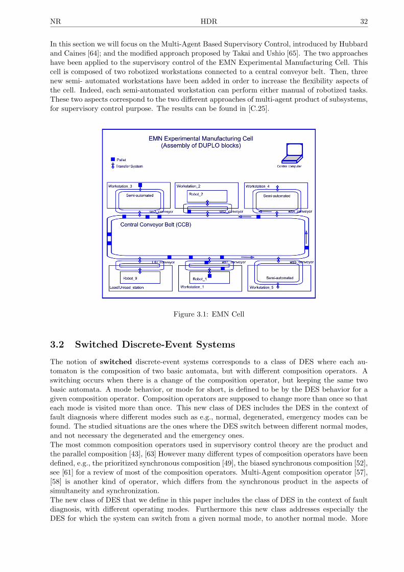
In this section we will focus on the Multi-Agent Based Supervisory Control, introduced by Hubbardand Caines [64]; and the modified approach proposed by Takai and Ushio [65]. The two approacheshave been applied to the supervisory control of the EMN Experimental Manufacturing Cell. Thiscell is composed of two robotized workstations connected to a central conveyor belt. Then, threenew semi- automated workstations have been added in order to increase the flexibility aspects ofthe cell. Indeed, each semi-automated workstation can perform either manual of robotized tasks.These two aspects correspond to the two different approaches of multi-agent product of subsystems,for supervisory control purpose. The results can be found in [C.25].
Figure 3.1: EMN Cell
3.2 Switched Discrete-Event Systems
The notion of switched discrete-event systems corresponds to a class of DES where each au-tomaton is the composition of two basic automata, but with different composition operators. Aswitching occurs when there is a change of the composition operator, but keeping the same twobasic automata. A mode behavior, or mode for short, is defined to be by the DES behavior for agiven composition operator. Composition operators are supposed to change more than once so thateach mode is visited more than once. This new class of DES includes the DES in the context offault diagnosis where different modes such as e.g., normal, degenerated, emergency modes can befound. The studied situations are the ones where the DES switch between different normal modes,and not necessary the degenerated and the emergency ones.The most common composition operators used in supervisory control theory are the product andthe parallel composition [43], [63] However many different types of composition operators have beendefined, e.g., the prioritized synchronous composition [49], the biased synchronous composition [52],see [61] for a review of most of the composition operators. Multi-Agent composition operator [57],[58] is another kind of operator, which differs from the synchronous product in the aspects ofsimultaneity and synchronization.The new class of DES that we define in this paper includes the class of DES in the context of faultdiagnosis, with different operating modes. Furthermore this new class addresses especially theDES for which the system can switch from a given normal mode, to another normal mode. More
NR HDR 33
precisely this new class of DES is an automaton which is the composition of two basic automata,but with different composition operators. A switching corresponds to the change of compositionoperator, but the two basic automata remains the same. A mode behavior (or mode for short)is defined to be the DES situation for a given composition operator. Composition operators aresupposed to change more than once so that each mode is visited more than once.
We give here below some examples of switched DES:
• Manufacturing systems where the operating modes are changing (e.g. from normal mode todegenerated mode)
• Discrete event systems after an emergency signal (from normal to safety mode)
• Complex systems changing from normal mode to recovery mode (or from safety mode tonormal mode).
We can distinguish, like for the switched continuous-time systems, the notion of autonomous switch-ing where no external action is performed and the notion of controlled switching, where the switchingis forced. The results for this section can be found in [55].
3.3 Switchable Languages of DES
The notion of switchable languages has been defined by Kumar, Takai, Fabian and Ushio in [Kumar-et-al. 2005]. It deals with switching supervisory control, where switching means switching betweentwo specifi- cations. In this paper, we first extend the notion of switchable languages to n languages,(n ≥ 3). Then we consider a discrete-event system modeled with weighted automata. The switchingsupervisory control strategy is based on the cost associated to each event, and it allows us tosynthesize an optimal supervisory controller. Finally the proposed methodology is applied to asimple example.
We now give the main results of this paper. First, we define a triplet of switchable languages.Second we derive a necessary and sufficient condition for the transitivity of switchable languages(n = 3). Third we generalize this definition to a n-uplet of switchable languages, with n > 3. Andfourth we derive a necessary and sufficient condition for the transitivity of switchable languages forn > 3.
3.3.1 Triplet of Switchable Languages
We extend the notion of pair of switchable languages, defined in [51], to a triplet of switchablelanguages.
Definition 2 (Triplet of switchable languages). A triplet of languages (K1,K2,K3), Ki ⊆ Lm(G)with Hi ⊆ Ki, i = {1, 2, 3} are said to be a triplet of switchable languages if they are pairwiseswitchable languages, that is,
SW (K1,K2,K3) := SW (Ki,Kj), i = j, i, j = {1, 2, 3}.
Another expression of the triplet of switchable languages is given by the following lemma.
Lemma 1 (Triplet of switchable languages). A triplet of languages (K1,K2,K3), Ki ⊆ Lm(G)with Hi ⊆ Ki, i = {1, 2, 3} are said to be a triplet of switchable languages if the following holds:
SW (K1,K2,K3) = {(H1,H2,H3) | Hi ⊆ Ki ∩ pr(Hj), i = j, and Hi controllable}.
NR HDR 34
3.3.2 Transitivity of Switchable Languages (n = 3)
The following theorem gives a necessary and sufficient condition for the transitivity of switchablelanguages.
Theorem 1 (Transitivity of switchable languages, n = 3) . Given 3 specifications (K1,K2,K3),Ki ⊆ Lm(G) with Hi ⊆ Ki, i = {1, 2, 3} such that SW (K1,K2) and SW (K2,K3).(K1,K3) is a pair of switchable languages, i.e. SW (K1,K3), if and only if
1. H1 ∩ pr(H3) = H1, and
2. H3 ∩ pr(H1) = H3.
The proof can be found in [42].
3.3.3 N-uplet of Switchable Languages
We now extend the notion of switchable languages, to a n-uplet of switchable languages, with(n > 3).
Definition 3 (N-uplet of switchable languages, n > 3). A n-uplet of languages (K1, ...,Kn), Ki ⊆Lm(G) with Hi ⊆ Ki, i = {1, ..., n}, n > 2, is said to be a n-uplet of switchable languages if thelanguages are pairwise switchable that is,
SW (K1, ...,Kn) := SW (Ki,Kj), i = j, i, j = {1, ..., n}, n > 2.
As for the triplet of switchable languages, an alternative expression of the n-uplet of switchablelanguages is given by the following lemma.
Lemma 2 (N-uplet of switchable languages, n > 3). A n-uplet of languages (K1, . . . ,Kn), Ki ⊆Lm(G) with Hi ⊆ Ki, i = {1, ..., n}, n > 3 are said to be a n-uplet of switchable languages if thefollowing holds:
SW (K1, ...,Kn) = {(H1, ..., Hn) | Hi ⊆ Ki ∩ pr(Hj), i = j, and Hi controllable}.
3.3.4 Transitivity of Switchable Languages (n > 3)
We are now able to derive the following theorem that gives a necessary and sufficient condition forthe transitivity of n switchable languages.
Theorem 2 (Transitivity of n switchable languages, n > 3) . Given n specifications (K1, ...,Kn),Ki ⊆ Lm(G) with Hi ⊆ Ki, i = {1, ..., n}. Moreover, assume that each language Ki is at leastswitchable with another language Kj , i = j.A pair of languages (Kk,Kl) is switchable i.e. SW (Kk,Kl), if and only if
1. Hk ∩ pr(Hl) = Hk, and
2. Hl ∩ pr(Hk) = Hl.
The proof is similar to the proof of Theorem 6 and can be found in [42]. It is to be noted that theassumption that each of the n languages be at least switchable with another language is important,in order to derive the above result. The results can be found in [C.sub1].
Chapter 4
Conclusion and Future Work
4.1 Summary of Contributions
In this HDR Thesis, I have presented a summary of contribution, in Analysis and Control of HybridSystems, as well as in Supervisory Control of Discrete-event Systems.
• Analysis and Control of Hybrid and Switched Systems
– Modeling and Control of MLD Systems
– Stability of Switched Systems
– Optimal Control of Switched Systems
• Supervisory Control of Discrete-Event Systems
– Multi-Agent Based Supervisory Control
– Switched Discrete-Event Systems
– Switchable Languages of DES
I have chosen to not present some work like the Distributed Resource Allocation Problem,the Holonic Systems, and the VMI-Inventory Control work. However the references of thecorresponding papers are given in the complete list of publications. My perspectives of research inthe coming years are threefold: 1) Control of Smart Grids, 2) Simulation with StochasticPetri Nets and 3) Planning and Inventory Control.
4.2 Perspective 1: Control of Smart Grids
According to the US Department of Energy’s Electricity Advisory Committee, ”A Smart Gridbrings the power of networked, interactive technologies into an electricity system, giving utilities andconsumers unprecedented control over energy use, improving power grid operations and ultimatelyreducing costs to consumers.”
The transformation from traditional electric network, with centralized energy production to com-plex and interconnected network will lead to a smart grid. The five main triggers of Smart grid,according to a major industrial point of view, are 1) Smart energy generation, 2) Flexible distribu-tion, 3) Active energy efficiency, 4) Electric vehicles, and 5) Demand response.From a control point of view, a smart grid is a system of interconnected micro-grids. A micro-grid is a power distribution network where generators and users interact. Generators technologiesinclude renewable energy such as wind turbines or photovoltaic cells.The objective of this project is to simulate and control a simplified model of a micro-gridthat is a part of a Smart Grid. After a literature review, a simplified model for control will bechosen. Different realistic scenarios will be tested in simulation with MATLAB. Finally different
35
NR HDR 36
Figure 4.1: Smart Grid
control strategies e.g. LQ/LQR Control, MPC and Hybrid Control will be tested in simulationwith MATLAB.
4.3 Perspective 2: Simulation with Stochastic Petri Nets
The Air France CDG Airport Hub in Paris-Roissy is dealing daily with 40,000 transfer luggagesand 30,000 local luggages (leaving from or arriving at CDG Airport). For this purpose Air Franceis exploiting the Sorting Infrastructure of Paris Aeroport, and has to propose a Logistical SchemeAllocation for each luggage in order to optimize the sorting and to minimize the number of failedluggages. By failed luggages, we mean a luggage that does not arrive in time for the assigned flight.The KPI Objective for 2017 is to have less than 20 failed luggages out of 1000 passengers.
Figure 4.2: CDG Airport Paris-Roissy
4.4 Perspective 3: Planning/Inventory Control
The strategy of integration known as VMI (Vendor-Managed Inventory) allows the coordination ofinventory policies between producers and buyers in supply chains. Based on a new proposed modelfor the implementation of VMI in a chain of two links composed of a producer and a buyer, thispaper studies the evolution of individual strategies of the producer and the buyer by a formalismderived from the theory of evolutionary games. The conditions that determine the stability ofevolutionarily stable strategies are derived and analyzed. Work results specify analytical conditionsthat favor the implementation of VMI on traditional chains without VMI.
References
37
NR HDR 38
References
[1] R. Alur, C. Courcoubetis, N. Halbwachs, T.A. Henzinger, P.-H. Ho, X. Nicollin, A. Olivero, J.Sifakis, and S. Yovine, ”The algorithmic analysis of hybrid systems,” Theoretical ComputerSci vol. 138, pp. 3-34, 1995.
[2] P.J. Antsaklis. ”A brief introduction to the theory and applications of hybrid systems,” Proc.of the IEEE, vol.88, no. 7, pp. 879-887, July 2000.
[3] A. Bemporad and M. Morari. ”Control of systems integrating logic, dynamics, and con-straints,”. Automatica, vol. 35 no. 3, pp. 407-427, 1999.
[4] A. Bemporad, G. Ferrari-Trecate, and M. Morari. ”Observability and controllability of PWAand hybrid systems,” IEEE Trans. on Automatic Control, vol. 45, no. 10, pp. 1864–1876, Oct.2000.
[5] A. Bemporad. ”An efficient technique for translating mixed logical dynamical systems intopiecewise affine systems,” in Proc. of 42nd IEEE Conf. Decision Control, 2002, pp. 1970-1975.
[6] A. Bemporad. ”Efficient conversion of mixed logical dynamical systems into an equivalentpiecewise affine form,” IEEE Trans. on Automatic Control, vol. 49, no. 5, pp. 832–838, May2004.
[7] V.D. Blondel and J.N. Tsitsiklis. ”Complexity of stability and controllability of elementaryhybrid systems,”. Automatica, vol. 35 no. 3, pp. 479-490, 1999.
[8] T. Geyer, F.D. Torrisi, and M. Morari. ”Efficient mode enumeration of compositional hybridsystems,” in Proc. of HSCC 2003, O. Maler and A. Pnueli (Eds.), LNCS 2623, pp. 216-232,2003.
[9] W.P.M.H. Heemels, B. de Schutter, and A. Bemporad. ”Equivalence of hybrid dynamicalmodels,” In Proc. of IEEE Symp. on Logic in Computer Science, New Brunswick, NJ, USA,pp. 278–292, 1996.
[10] T.A. Henzinger. ”The theory of hybrid automata,” Proc. of the 11th Annual Symp. on LICS,pp. 278-292, IEEE Computer Society Press, 1996.
[11] H. Lin and P.J. Antsaklis. ”Stability and stabilizability of switched linear systems: A shortsurvey of recent results,” in Proc. Int. Symp. on Intelligent Control, Limassol, Cyprus, June2005, pp. 24-29.
[12] M. Margaliot. ” Stability analysis of switched systems using variational principles,”. Auto-matica, vol. 42, pp. 2059-2077, 2006.
[13] A. Rantzer and M. Johansson. ”Piecewise linear quadratic optimal control of hybrid systems,”IEEE Trans. on Automatic Control, vol. 45, no. 4, pp. 629–637, April 2000.
[14] C. Seatzu, D. Corona, A. Giua, and A. Bemporad. ”Optimal control of continuous-timeswitched affine systems,” IEEE Trans. on Automatic Control, vol. 49, no. 5, pp. 726–741, May2006.
39
NR HDR 40
[15] E.D. Sontag. ”Nonlinear regulation: The piecewise affine approach,” IEEE Trans. on Auto-matic Control, vol. 51, no. 5, pp. 346-358, April 1981.
[16] Z. Sun and S.S. Ge. ”Analysis and synthesis of switched linear control systems,”. Automatica,vol. 41, pp. 181-195, 2005.
[17] F.D. Torrisi and A. Bemporad. ”HYSDEL– A tool for generating computational hybrid mod-els,”. IEEE Trans. Control System Technology, Vol. 12, N.2, pp. 235-249, Mar 2004.
[18] D. Liberzon, ”Switching in Systems and Control,” Birkhauser, Boston, 2003.
[19] H. Lin, P.J. Antsaklis. ”Stability and stabilizability of switched linear systems: A survey ofrecent results” IEEE Transactions on Automatic Control , vol.54, no. 2, pp. 308–322, 2009.
[20] W. Dayawansa, C. Martin, ” A converse Lyapunov theorem for a class of dynamical systemswhich undergo switching” IEEE Transactions on Automatic Control , vol. 44 N. pp.751–760,1999.
[21] J. Mancilla-Aguilar, R. Garcia, ”A converse Lyapunov theorem for nonlinear switched sys-tems,” Systems and Control Letters, vol. 41 N. 1 pp.67–71, 2000.
[22] L. Vu, D. Liberzon, ”Common Lyapunov functions for families of commuting nonlinear sys-tems” Systems and Control Letters, vol. 54 N. 1 pp. 405–416, 2005.
[23] C. Ebenbauer, F. Allgwer, ”Stability analysis of constrained control systems: An alternativeapproach,” Systems and Control Letters, vol. 56 pp. 93–98, 2007.
[24] A. Papachristodoulou, S. Prajna, ”Analysis of non-polynomial systems using the sum ofsquares decomposition,” Positive Polynomials in Control Springer, pp. 23–43, 2005.
[25] P. Kunkel, V. Mehrmann, ”Stability properties of differential-algebraic equations and spin-stabilized discretizations,” Electronic Transactions on Numerical Analysis vol. 26, 385–420,2007.
[26] S. Prajna, A. Papachristodoulou, ”Analysis of switched and hybrid systems?Beyond piecewisequadratic methods Proc. of the American Control Conference, Boston, MA, USA, pp. 1208-1213, July 2004.
[27] S. C. Bengea and R. A. DeCarlo ”Optimal control of switching systems”. Automatica, vol. 41,pp. 11–27, 2005.
[28] J.B. Lasserre, ”Global optimization with polynomials and the problem of moments.”. SIAMJ. Optimization, vol. 11, pp. 796-817, 2001.
[29] J.B. Lasserre, C. Prieur, D. Henrion, ”Nonlinear optimal control: numerical approximationvia moments and LMI relaxations.”. Proc. of the Joint IEEE CDC and ECC 2005, Sevilla,Spain, Dec. 2005.
[30] J.B. Lasserre, D. Henrion, C. Prieur, E. Trelat, ”Nonlinear optimal control via occupationmeasures and LMI relaxations.”. SIAM J. Control and Optimization, vol. 47 N. 4, pp. 1643-1666, 2008.
[31] D. Liberzon, ”Switching in Systems and Control,” Birkhauser, Boston, 2003.
[32] R. Meziat, D. Patino, and P. Pedregal, ”An alternative approach for non-linear optimal controlproblems based on the method of moments, ”. Computational Optimization and Applications,vol. 38, pp. 147–171, 2007
NR HDR 41
[33] P. Parrilo, ”Structured semidefinite programs and semi-algebraic geometry methods in robust-ness and optimization. ”. Ph.D. Thesis, California Institute of Technology, 2000.
[34] D. Patino, P. Riedinger, and C. Iung, ” Optimal state feedback control law for continuous-timeaffine switched systems.,” 2007.
[35] P. C. Perera and W. P. Dayawansa, ”Asymptotic feedback controllability of switched controlsystems to the origin,” Proc. of the American Control Conference, pp. 5806–5811, 2004.
[36] P. Riedinger, J. Daafouz, and C. Iung, ”Suboptimal switched controls in context of singulararcs,” Proc. of 42nd IEEE Conference on Decision and Control, 6254–6259, 2003.
[37] W. Spinelli, P. Bolzern, and P. Colaneri, ”A note on optimal control of autonomous switchedsystems on a finite time interval,” Proc. of the American Control Conference, 2006.
[38] K. C. Toh, M. J. Todd, and R. Tutuncu, ”SDPT3 ? A Matlab software package for semidefiniteprogramming, ” Optimization Methods and Software, vol.11, pp. 545–581, 1999.
[39] X. Xu, P.J. Antsaklis. ”Optimal control of switched systems based on parameterization of theswitching instants, ” IEEE Transactions on Automatic Control , vol.49, pp. 2–16, 2004.
[40] S.E. Bourdon, M. Lawford, and W.M. Wonham ”Robust nonblocking supervisory control ofdiscrete event systems,” In IEEE Trans. on Automatic Control, vol. 50, N.12 pp. 2015–2021,2005.
[41] M. Canu and N. Rakoto-Ravalontsalama, From mutually non-blocking to switched non-blockingDES. Presented at MSR’13 Workshop (Poster Session), Rennes, France, Nov 13-15, 2013.
[42] M. Canu and N. Rakoto-Ravalontsalama. On Switchable Languages of Discrete-Event Systemswith Weighted Automata, Technical Report Mines Nantes, March 2017.
[43] C.G. Cassandras and S. Lafortune, ”Introduction to Discrete Event Systems,” 2nd Edition,Springer Verlag, 2008.
[44] M. Fabian and R. Kumar. ”Mutually non-blocking supervisory control of discrete-eventsystems,” In Automatica, 36(12) pp. 1863–1869, 2000.
[45] G. Faraut, L. Pietrac, and E. Niel, ”Formal Approach to Multimodal Control Design: Appli-cation to Mode Switching”, In IEEE Trans. on Industrial Informatics, vol.5, N.4 pp. 443–453,Nov 2009.
[46] G. Faraut, L. Pietrac, and E. Niel, ”Process Tracking by Equivalent States in Modal Super-visory Control”, Proc. of IEEE ETFA, Sep. 2011, Toulouse, France.
[47] J. Girault, J.J. Loiseau, O.H. Roux ”Synthese en ligne de superviseur compositionnel pour uneflotte de robots mobiles.” European Journal of Automation, MSR’13, vol 47/1-3, pp. 195–210,2013.
[48] J. Girault, J.J. Loiseau, O.H. Roux ”On-line optimal compositional controller synthesis forAGV by unfolding,” Proc. of DCDS 2015, IFAC-PapersOnLine 48-7 (2015) pp. 167–173.
[49] M. Heymann, ”Concurrency and discrete event control,” In IEEE Control Systems Magazine,vol 10, N.4 pp. 103–112, 1990.
[50] J.E. Hopcroft and J.D. Ullman, ”Introduction to Automata Theory, Languages, and Compu-tation,” Addison-Wesley, Reading, MA, USA, 1979.
NR HDR 42
[51] R. Kumar, S. Takai, M. Fabian, and T. Ushio, ”Maximally Permissive Mutually and GloballyNonblocking Supervision with Application to Switching Control,” In Automatica, 41(8) pp.1299–1312, 2005.
[52] S. Lafortune, E. Chen, ”The infimal closed controllable superlanguage and its application tosupervisory control, ” IEEE Transactions on Automatic Control , vol.35, N.4, pp. 398–405,1990.
[53] D. Liberzon, ”Switching in Systems and Control”, ser. Systems and Control: Foundations andApplications. Boston: Birkhauser, 2003.
[54] R. Malik and R. Leduc, ”Generalised nonblocking”’, in Proc. 9th Int. Workshop on DiscreteEvent Systems, WODES 2008, Goteborg, Sweden, May 2008, pp. 340–345.
[55] N. Rakoto-Ravalontsalama. ”Supervisory control of switched discrete-event systems,” in Proc.of 17th Symp. on MTNS 2006, Kyoto, Japan 2006, pp. 2213–2217.
[56] P.J. Ramadge and W.M. Wonham. ”Supervisory control of a class of discrete-event processes,”In SIAM J. Control and Optimization, vol.25 pp. 206–230, 1987.
[57] I. Romanovski , P.E. Caines, ”On the supervisory control of multi-agent product systems,”Proc. of IEEE Conference on Decision and Control, Las Vegas, Nevada, pp. 1181-1186, 2002.
[58] I. Romanovski , P.E. Caines, ”Multi-agent product system: Controllability and non-blockingproperties,” Proc. of WODES 2006, Ann Arbor, MI, 2006.
[59] P.S. Roop, A. Girault, R. Sinha, and G. Goessler. ”Specification Enforcing Refinement forConvertibility Verification,” Proc. of ACSD 2009, pp. 148–157, IEEE, 2009.
[60] T.J.J. van den Boom and B. de Schutter. ”Modelling and control of discrete event systemsusing switching max-plus-linear systems,” Control Engineering Practice, vol. 14 N.10, pp.1199-1211, 2006.
[61] F. Wenck, J.H. Richter, ”On composition oriented perspective on controllability of large DES,”Proc. of WODES 2004, Reims, France, pp. 271–276, 2004.
[62] W.M. Wonham and P.J. Ramadge. ”Modular supervisory control of discrete-event systems,”In Mathematics of Control, Signals and Systems, vol.1 (1) pp. 13–30, 1988.
[63] W.M. Wonham, ”Notes on Discrete Event Systems,” Dept. of ECE, University of Toronto,Toronto, Canada, 2004.
[64] P. Hubbard and P.E. Caines, ”Initial investigations on hierachical supervisory control ofmulti-agent systems,” Proc. of IEEE Conference on Decision and Control, Phoenix, AZ, pp.2218–2223, 1999.
[65] S. Takai and T. Ushio, ”Supervisory control of a class of concurrent discrete-event systems,”Proc. of ATPN - Workshop on DES Control, Eindhoven, The Netherlands,, pp. 37?55, June2003
Appendix A
Appendix 1 – Paper [C.24]:
• [C.24] J.L. Villa, M. Duque, A. Gauthier, and N. Rakoto-Ravalontsalama,A new algorithm for translating MLD systems into PWA systems.Proc. of IEEE American Control Conference (ACC 2004), June 30 - July 2,2004, Boston, MA, USA, pp. 1208 –1213.
43
NR HDR 44
A New Algorithm for Translating MLD Systems into PWA Systems
J.L. Villa1,2, M. Duque2, A. Gauthier2 and N. Rakoto-Ravalontsalama1
1Ecole des Mines de Nantes / IRCCyN 4, rue Alfred Kastler, F-44307 Nantes Cedex 03, France
{jvilla, rakoto}@emn.fr 2Universidad de los Andes
Kra 65B No 17A-11, Bogotá D.C., Colombia {maduque, agauthie}@uniandes.edu.co
Abstract − This paper presents a new algorithm for
translating Mixed Logical and Dynamical (MLD) systems into PieceWise Affine (PWA) systems. The presented algorithm uses an enumeration technique and solves several linear programming problems in order to obtain the equivalence. The obtained model is equivalent to the MLD model meaning that given an initial state and an input sequence, the trajectory of the state vector and output vector are the same. The technique is applied to three examples. The computation time and the simulation results for these examples are given.
I. INTRODUCTION
Mixed and Logical Dynamical (MLD) models introduced by Bemporad and Morari in [2] arise as a suitable representation for Hybrid Dynamical Systems (HDS), in particular for solving control-oriented problems. MLD models can be used for solving a model predictive control (MPC) problem of a particular class of HDS and it is proved that MLD models are equivalent to PieceWise Affine Models in [6]. In the paper by Heemels and co-workers, the equivalencies among PieceWise Affine (PWA) Systems, Mixed Logical and Dynamical (MLD) systems, Linear Complementarity (LC) systems, Extended Linear Complementarity (ELC) systems and Max-Min-Plus-Scaling (MMPS) systems are proved, these relations are transcribed here in Fig. 1.
This equivalences are based on some propositions (see [6] for details)
Fig. 1. Equivalence relation between hybrid systems Every well-posed PWA system can be re-written as an
MLD system assuming that the feasible states and inputs are bounded [6, proposition 4*]. A completely well-posed MLD system can be rewritten as a PWA system [6, proposition 5*].
A more formal proof can be found in [3], where an efficient technique for obtaining a PWA representation of a MLD model is proposed.
The technique in [3] describes a methodology for obtaining, in an efficient form, a partition of the state-input space. The algorithm in [3] uses some tools from polytopes theory in order to avoid the enumeration of the all possible combinations of the integer variables contained in the MLD model. However, the technique does not describe the form to obtain a suitable choice of the PWA model, even though this part is introduced in the implementation provided by the author in [4]. The objective of this paper is to propose an algorithm of the suitable choice of the PWA description and use the PWA description for obtaining some analysis and control of Hybrid Dynamical Systems.
II. MLD SYSTEMS AND PWA SYSTEMS
A. Mixed and Logical Dynamical (MLD) Systems The idea in the MLD framework is to represent logical
propositions as equivalent integer expressions. MLD form is obtained by three basic steps [5]. The first step is to associate a binary variable δ ∈{0,1} with a proposition S, that may be true or false. δ is 1 if and only if proposition S is true. A composed proposition of elementary propositions S1,…,Sq combined using the boolean operators like AND(^), OR (∨), NOT(~) may be expressed like integer inequalities over corresponding binary variables δi, i=1,…,q.
The second step is to replace the products of linear functions and logic variables by a new auxiliary variable z = δaTx where aT is a constant vector. The z value is obtained by mixed linear inequalities evaluation.
The third step is to describe the dynamical system, binary variables and auxiliary variables in a linear time invariant (LTI) system.
A hybrid system MLD described in general form is represented by (1).
1 2 3
1 2 3
2 3 1 4 5
( 1) ( ) ( ) ( ) (
( ) ( ) ( ) ( ) ( )
( ) ( ) ( ) ( )
x k Ax k B u k B k B z k
y k Cx k D u k D k D z k
E k E z k E u k E x k E
δ
δ
δ
+ = + + + = + + + + ≤ + +
) (1)
where l are the continuous and [ ] {0,1}cT T n nC lx x x= ∈ ×R
binary states, u u are the inputs, the outputs, and , ,
represent the binary and continuous auxiliary variables, respectively. The constraints over state, input, output, z and δ variables are included in the third term in (1).
[ ] {0,1}cT T m mC lu= ∈ ×R
{0,1}c lp×
, ,i i i
ii i i
x a B ux u X i
x c D u
= + +× ∈ ∈
= + +
) ( ),
( )i i i
ii i i
b B u kx u
d D u k
+ +×
+
l)
[ ]T T pC ly y y= ∈ R
x A
y C
( 1) (
( ) ( )
x k Ax k
y k C x k
+ = = +
{0,1} lrδ ∈
, t +∈Ι
,X i k∈ ∈ I
crz ∈ R
, +∈ Z
B. PieceWise Affine Systems
A particular class of hybrid dynamical systems is the system described as follows,
(2)
where I is a set of indexes, Xi is a sub-space of the real
space Rn, and R+ is the set of positive real numbers
including the zero element. In addition to this equation it is necessary to define the
form as the system switches among its several modes. This equation is affine in the state space x and the systems described in this form are called PieceWise Affine Systems (PWA). In the literature of hybrid dynamical systems the systems described by the autonomous version of this representation are called Switched Systems.
If the system vanishes when x brings near to zero, i.e. ai and bi are zero, then the representation is called PieceWise Linear (PWL) system.
The discrete-time version of this equation will be used in this work and can be described as follows,
(3)
where I is a set of indexes, Xi is a sub-space of the real
space Rn.
III. MLD SYSTEMS INTO PWA SYSTEMS
The MLD framework is a powerful structure for representing hybrid systems in an integrated form. Although E1, E2, E3, E4 and E5 matrices are, in general, large matrices, they can be obtained automatically. An example is the HYSDEL compiler [10].
However, some analysis of the system with the MLD representation are computationally more expensive with respect to some tools developed for PWA representations. Exploiting the MLD and PWA equivalencies, it is possible to obtain analysis and control of a system using this equivalent representations. Nevertheless, as it is underlined in [3], this procedure is more complex with respect to the PWA into MLD conversion, and there exist more assumptions. To our knowledge, the only previous approach has been proposed by Bemporad [3]. We propose then a new approach of translating MLD into PWA systems.
The MLD structure can be rewritten as follows,
1 1 2 3
1 1 2 3
2 3 2 1 1 5
( )( 1) ( ) ( ) (
( )
( )( ) ( ) ( ) ( )
( )
( )( ) ( ) ( )
( )
cc l
l
cc l
l
cc l
l
u kx k Ax k B B B k B z k
u k
u ky k Cx k D D D k D z k
u k
u kE k E z k E x k E E E
u k
δ
δ
δ
+ = + + + = + + + + ≤ + +
(4)
Here, the binary inputs are distinguished from the continuous inputs, because they induce switching modes in the system, in general.
Supposing that the system is well posed, z(k) has only one possible value for a given x(k) and u(k), and can be rewritten as:
1 2 3( ) ( ) ( ) | [ , ]T T Tcz k k x k k u k k m x u b= + + ≤ (5)
Replacing this value in the original equations the system can be represented as,
3 1 1 3 2 3 3
3 1 1 3 2 3 3
4 3 1 1 3 2 5 2 3 3
( 1) ( ) ( ) ( ) ( )
( 1) ( ) ( ) ( ) ( )
( ) ( )
c
c
x k A B k x k B B k u k B k
y k C D k x k D D k u k D k
E E k x E E k u E E E kδ
+ = + + + + + = + + + + − + + − + ≤ − −
(6)
If an enumeration technique is used for generating all the feasible binary states of the [ul
T δT]T vector, the first problem is to find a value of [xT uT]T feasible for the problem, that can be obtained solving the linear programming problem,
1 3 4 5 2 1
min [ ]
. .
T T T T
c c l l
X u z x
s t E u E z E x E E E uδ
= − + − ≤ − +
(7)
The solution is a feasible value [x*T u*T]T. The next problem is to find k1, k2 and k3.
The inequalities can be rewritten as,
3 4 1 1 2 5 4 1 1 2 5c c l l c cE z E x E u E u E E E k x E k u E kδ≤ + + − + = + + 3 (8)
where 5E includes every constant in the problem, i.e. ul and δ. On the other hand, the E3 matrix reflects the interaction among the z variables, and we can write:
1 2F z k x k u k3× ≤ + + (9)
The matrix F represents the interaction among the z variables, if the system is well posed F-1 should exist.
With this last equation, for finding 3k the next linear programming problem is solved,
3
* *3 3 5 2 1
max
. . l l
k
s t E k E E E uδ
≤ − +
(10)
The solution to this problem is 3k , in this case we assume that all components in 5E are the maximum and minimum values of z and the only solution for the problem is 3k . With 3k we can obtain the other matrices.
For obtaining 1k it is necessary to solve nx, i.e. the
length of the state vector, linear programming problems,
* *3 5 2 1
max
. .
i
i l
k
s t E k E E E u Eδ
≤ − + + 4l i
(11)
where E4i represents the column i of the E4 matrix and 1i ik k= − 3k is the column i of the matrix 1k .
For obtaining 2k it is necessary to solve nu, i.e. the length of the continuous input vector, linear programming problems,
* *3 5 2 1
max
. .
i
i l
k
s t E k E E E u Eδ
≤ − + + 1l ci
(12)
where E1ci represents the column i of the E1c matrix and 2i ik k k= − 3 is the column i of the matrix 2k .
The matrix F should be found solving nz, i.e. the length of the z vector, linear programming problems,
* *3 5 2 1
max
. .
i
i l
k
s t E k E E E u Eδ
≤ − + + 3l i
(13)
where E3i represents the column i of the E3 matrix and 3i iF k k= − is the column i of the matrix . F
Finally, k1, k2, and k3, can be computed as, 1
1
12 2
13 3
k F k
k F k
k F k
−
−
−
= = =
1 (14)
With these equations, the algorithm for translating the MLD model into PWA model is given as follows, Algorithm 1 1. Find a feasible point for the binary vector,
composed by the binary inputs and binary auxiliary variables.
2. Compute 3k using Eq. (10). 3. Compute 1k , 2k and F using Eq. (11), (12) and
(13). 4. Compute k1, k2, and k3 using Eq. (14). 5. Using Eq. (6), compute Ai, Bi, fi, Ci, Di and gi and
the valid region for this representation. 6. If there exists another feasible point go to
step 1. 7. End.
Some gains in the algorithm performance can be obtained if the vector z is evaluated after step one, using a linear program for finding the maximum and the minimum in z, if the zmin and zmax solutions are the same, it is not necessary to calculate steps 3, and 4, and z = zmin = zmax can be assigned directly.
IV. EXAMPLES
A. The Three-Tank Benchmark Problem The three-tank benchmark problem has been proposed as
an interesting hybrid dynamical system. This Benchmark was proposed in [7] and [8]. See [13] and references there in for some control results using MLD framework in this system. The algorithm described in the last section is used for obtaining a PWA representation of this system.
This system has three tanks each of them interconnected with another as depicted in Fig. 2.
Fig. 2. Three Tank System
The model is written using binary variables (δi) and
relational expressions, 01 1 11 1
2 2 02 2
3 3 03 3 3
( )1
1 (
1 ( )
vv
v v
v v
Z h hh h
h h Z h h
h h Z h h
δδ
δ δ
δ δ
= −= ↔ > = ↔ > = − = ↔ > = −
2)
1
2
1 01 03
2 02 03
13 1 3 13
23 2 3 23
( )
( )
( )
( )
Z Z Z V
Z Z Z V
Z h h V
Z h h V
= − = − = − = −
1 1 13 11 1
1 1 13 1 1
( ) ( ) ( ) ( )( 1) ( ) * (s
L
q k h k Z k Z kh k h k T
C R C R C RC+ = + − − −
1)
2 23 22 2
2 23 2 2
( ) ( ) ( )( 1) ( ) * (
q k Z k Z kh k h k Ts
C R C R C+ = − − −
2
3 13 23 1 23 3
3 13 3 23 2 1 3 2
( ) ( ) ( ) ( ) ( )( 1) ( ) * (
N
h k Z k Z k Z k Z kh k h k Ts
R C R C R C RC RC+ = + − + + + +
3)
)
The simulation of the system using the MLD framework and a Mixed Integer Quadratic Programming MIQP algorithm running in an Intel Celeron 2GHz processor and 256MB of RAM was 592.2s, using the PWA representation the same simulation was 1.33s. The time for obtaining the PWA model using the technique described in this work is 72.90s and the algorithm found 128 regions. Using the algorithm in [4] the computation time of the PWA form was 93.88s and the total regions found was 100 and the simulation took 5.89s. These results are summarized in Table I.
Where Computation Time is the time taken by the computer for computing the PWA model based in the MLD model, and Simulation Time is the time taken by the
computer for computing a trajectory given a model, an initial state and an input sequence.
Table I. Computation and Simulation Times
Representation Computation
Time (s.) Simulation Time (s.)
MLD - 592.20PWA-[4] 93.88 5.89
PWA-This work 72.90 1.33 The simulation results with MLD model and the error
between PWA simulation results and MLD simulation results, for the same input are shown in Fig. 3,
(a) MLD Model (b) Error between MLD and PWA [4]
(C) Error between MLD and PWA– This Work
Fig. 3. Simulation Results for the Three-Tank System In this case, at t=30s, the simulation with the PWA system in the Figure 3.b produces a switching to an invalid operation mode. B. Car with Robotized Manual Gear Shift
The example of a Hybrid Model of a Car with Robotized Manual Gear Shift was reported in [9] and is used in [3] as example. The car dynamics is driven by the following equation,
e bmx F F xβ= − − (15) where m is the car mass, x and x is the car speed and
acceleration, respectively, Fe is the traction force, Fb is the brake force and β is the friction coefficient. The Transmission Kinematics are given by,
( )
( )
g
s
ge
s
R ix
kR i
F Mk
ω =
=
where ω is the engine speed, M the engine torque and i is the gear position.
The engine torque M is restricted to belongs between the minimum engine torque C and the maximum engine torque C .
( )e ω−
( )e ω+
The model has two continuous states, position and velocity of car, two continuous inputs, engine torque and breaking force, and six binary inputs, the gear positions. The MLD model was obtained using the HYSDEL tool.
The translation of the MLD model took 155.73 s and the PWA model found 30 sub-models, using the algorithm proposed in this work, and the PWA model using the algorithm proposed in [3] took 115.52 s and contains 18 sub-models. The simulation time with MLD model and a MIQP algorithm for 250 iterations took 296.25s, using the PWA model obtained with the algorithm proposed here took 0.17s, and using the PWA model obtained using the algorithm in [4] the simulation took 0.35s. These results are summarized in Table II,
Table II. Computation and Simulation Times
Representation Computation
Time (s.) Simulation
Time (s.) MLD - 296.25
PWA-[4] 115.52 0.35PWA-This work 155.73 0.17
The simulation results with MLD model and the error
between PWA simulation results and MLD simulation results, for the same input are shown in Fig. 4,
(a) MLD Model (b) Error between MLD and PWA [4]
(c) Error between MLD and PWA– This Work
Fig. 4. Simulation results for robotized gear shift
C. The Drinking Water Treatment Plant The example of a Drinking Water Treatment Plant has
been reported in [11] and [12]. This plant was modeled using identification techniques for hybrid dynamical systems, and its behavior includes autonomous jumps.
The plant modeled is based in the current operation of drinking water plant Francisco Wiesner situated at the periphery of Bogotá D.C. city (Colombia), which treats on average 12m3/s. The volume of water produced by this plant is near to 60% of consumption by the Colombian capital. In this plant, there exist two water sources: Chingaza and San Rafael reservoirs which can provide till 22m3/s of water.
The process mixes inlet water with a chemical solution in order to generate aggregated particles that can be caught in a filter. The dynamic of the filter is governed by the differential pressure across the filter and the outlet water turbidity. An automaton associated to the filter executes a back-washing operation when the filter performance is degraded. Because of process non-linearity, the behavior of the system is different with two water sources, that is the case for the particular plant modeled.
The model for each water source includes a dynamic for the aggregation particle process which dynamical variable is called Streaming Current (SC) and is modeled using two state variables, a dynamic for the differential pressure called Head Loss (HL) with only one state variable, a dynamic for the outlet turbidity (To) with two state variables.
The identified model consists of four affine models, two for each water source in normal operation, one model in maintenance operation, one model representing the jump produced at the end of the maintenance operation.
( 1) ( ) ( )
( ) ( ) ( )
{1, if water source1andnormal operation,
2, if water source2andnormal operation,
3, if maintenance operation,
4, change from maintenance operation
i i i
i i i
x k Ax k B u k f
y k C x k D u k g
i
+ = + + = + +∈
to normal operation}
where water source is an input variables, maintenance operation is executed if outlet turbidity (To) is greater than a predefined threshold, or, Head Loss (HL) is greater than a predefined threshold, or, operation time is greater than a predefined threshold.
The MLD model has 7 continuous states (including two variables for two timers in the automaton), 4 continuous inputs (dosage, water flow, inlet turbidity and pH), 3 binary inputs (water source, back-washing operation and normal operation), 8 auxiliary binary variables, and 51 auxiliary variables. The complete model can be obtained by mail from the corresponding authors.
The translation from the MLD model into PWA model
took 572.19 s, with the algorithm proposed here, generating 127 sub-models. The translation into PWA model took 137.37s, with the algorithm in [3], generating 14 sub-models. The simulation time for 300 iterations with the MLD model and a MIQP algorithm took 4249.301s, the same simulation with the PWA model obtained with the algorithm proposed here took 0.14s, and the same simulation with the PWA model obtained using the algorithm in [4] took 0.31s. These results are summarized in Table III,
Table III. Computation and Simulation Times.
Representation Computation
Time (s.) Simulation
Time (s.)MLD - 4249.30
PWA-[4] 137.37 0.31PWA-This work 572.20 0.14
The simulation results for the same input are shown in
Fig. 5,
(a) MLD Model (b) Error between MLD and PWA [4]
(c) Error between MLD and PWA– This Work
Fig. 5. Simulation results for a water plant model.
In this case, at t=168min, the simulation with the PWA system in the Figure 5.b is not valid because there exist no mode in the PWA representation that belongs to the state-input vector reached in this point. Some other results can be found in [14].
V. CONCLUSIONS This work presents new algorithm for obtaining a
suitable choice of the PWA description from a MLD representation. The results are applied to the three-tank
benchmark problem, to a car with robotized gear shift and to a drinking water plant, the three examples have been reported in the literature as examples of hybrid dynamical systems modeled with MLD formalism. The simulation results show that the PWA models obtained have the same behavior with respect to the MLD models. However in some cases the obtained PWA model does not have a valid solution for some state-input sub-spaces. As a consequence of the enumeration procedure, our PWA models have more submodels/regions than the algorithm in [3], however we show that the procedure does not spent much more computation time because of the simplicity in its formulation, and it ensures the covering of all regions included in the original MLD model.
Ongoing work concerns the analysis of MLD Systems with some results from PWA systems.
VI. ACKNOWLEDMENT This work has been supported in part by « Contrat Etat - Région No STIC 9-18036, 2000-2006 », Nantes, France. The authors are thankful to the reviewers for their valuable comments and suggestions.
VII. REFERENCES
[1] R. Alur, C. Courcoubetis, T. A. Henzinger, and P. H. Ho. Hybrid Automata : An Algorithmic Approach To The Specification and Verification of Hybrid Systems. In Hybrid Systems I, Lecture Notes in Computer Science 736, Springer-Verlag, pp. 209-229, 1993
[2] A. Bemporad and M. Morari. Control of Systems Integrating Logic, Dynamics, and Constraints. Automatica 35, pp. 407-427, 1999.
[3] A. Bemporad. An Efficient Technique for Translating Mixed Logical Dynamical Systems into PieceWise Affine Systems. Proceedings of the 41st IEEE Conference on Decision and Control. Las Vegas, Nevada USA, December 2002.
[4] A. Bemporad. An Efficient Technique for Translating Mixed Logical Dynamical Systems into PieceWise Affine Systems. Implementation. http://www.dii.unisi.it/~hybrid/tools/mld2pwa
[5] G. Ferrari-Trecate, D. Mignone, D. Castagnoli, and M. Morari. Hybrid Modeling and Control of a Hydroelectric
Power Plant. Technical Report AUT00-11, Automatic Control Laboratory, ETH Zurich, Switzerland, 2000.
[6] W.P.M.H. Heemels, B. de Schutter, and A. Bemporad. Equivalence of Hybrid Dynamical Models. Automatica, 37(7), pp. 1085-1091, July 2001.
[7] B. Heiming, J. Lunze Definition of the Three-Tank Benchmark Problem for Controller Reconfiguration. European Control Conference, 1999.
[8] J. Lunze. Benchmark for the Reconfiguration Problem: Laboratory 3 Tank System. Technical University Hamburg-Harbur. 1998. http://www.tu-arburg.de/rts/software/cosy
[9] F.D. Torrisi and A. Bemporad. Discrete-Time Hybrid Modeling and Verification. In Proc. 40th IEEE Conf. On Decision and Control, pp. 2899-2904 Orlando, Florida, 2001.
[10] F.D. Torrisi and A. Bemporad. HYSDEL Modeling and Simulation of Hybrid Dynamical Systems. Proceedings of MATHMOD Conference, Vienna University of Technology, Viena, Austria, February 5-7, 2003.
[11] J.L. Villa, M. Duque, A. Gauthier and N. Rakoto-Ravalontsalama Hybrid Modeling of Potable Water Treatment Plant. In : Cabrera and Cabrera Jr. (Eds.) Pumps, Electromechanical Devices and Systems : Applied to Urban Water Management. A.A. Balkema Publishers. Lisse, pp. 909-917. 2003.
[12] J.L. Villa, M. Duque, A. Gauthier and N. Rakoto-Ravalontsalama. Modeling and Control of a Water Treatment Plant. In: IEEE International Conference on Systems, Man & Cybernetics (SMC2003) October 5–8, Washington D.C., USA, pp. 171-176 (CD-ROM), 2003.
[13] J.L. Villa, M. Duque, A. Gauthier and N. Rakoto-Ravalontsalama. MLD Control of Hybrid Systems : Application to the Three-Tank Benchmark Problem. In : IEEE International Conference on Systems, Man & Cybernetics (SMC2003) October 5–8, Washington D.C., USA, pp. 666-671 (CD-ROM) 2003.
[14] J.L. Villa, M. Duque, A. Gauthier and N. Rakoto-Ravalontsalama. A New Algorithm for Translating MLD Systems into PWA Systems. Technical Report No 03/8/AUTO Ecole des Mines de Nantes, France. Sept. 2003.
Appendix B
Appendix 2 – Paper [J.5]:
• [J.5] E. Mojica, N. Quijano, and N. Rakoto-Ravalontsalama.A polynomial approach for optimal control of switched nonlinear systems,Int. Journal of Robust and Nonlinear Control, Wiley, 2014, 24 (12), pp.1797-1808.
51
NR HDR 52
INTERNATIONAL JOURNAL OF ROBUST AND NONLINEAR CONTROLInt. J. Robust. Nonlinear Control (2013)Published online in Wiley Online Library (wileyonlinelibrary.com). DOI: 10.1002/rnc.2964
A polynomial approach for optimal control of switchednonlinear systems
Eduardo Mojica-Nava1,*,†, Nicanor Quijano1 and Naly Rakoto-Ravalontsalama2
1Universidad de Los Andes, Cra 1 No. 18A-10, Bogotá, Colombia2Ecole des Mines de Nantes and IRCCyN, 44307 Nantes Cedex 03, France
Received 4 May 2012; Revised 7 November 2012; Accepted 21 December 2012
KEY WORDS: method of moment; optimal control; switched systems
1. INTRODUCTION
Switched nonlinear control systems are characterized by a set of several continuous nonlinear statedynamics with a logic-based controller, which determines simultaneously a sequence of switchingtimes and a sequence of modes. As performance and efficiency are key issues in modern techno-logical system such as automobiles, robots, chemical processes, power systems among others, thedesign of optimal logic-based controllers, covering all those functionalities while satisfying physicaland operational constraints, plays a fundamental role. In the last years, several researchers have con-sidered the optimal control of switched systems. An early work on the problem is presented in [1],where a class of hybrid-state continuous-time dynamic system is investigated. Later, a generaliza-tion of the optimal control problem and algorithms of hybrid systems is presented [2]. The particularcase of the optimal control problem of switched systems is presented in [3] and [4]. However, mostof the efforts have been typically focused on linear subsystems [5]. In general, the optimal controlproblem of switched system is often computationally hard as it encloses both elements of opti-mal control as well as combinatorial optimization [6]. In particular, necessary optimality conditionsfor hybrid systems have been derived using general versions of the Maximum Principle [7, 8] andmore recently in [9]. In the case of switching systems [4] and [6], the switched system has beenembedded into a larger family of systems, and the optimization problem is formulated. For generalhybrid systems, with nonlinear dynamics in each location and with autonomous and controlledswitching, necessary optimality conditions have recently been presented in [10]; and using theseconditions, algorithms based on the hybrid Maximum Principle have been derived. Focusing onreal-time applications, an optimal control problem for switched dynamical systems is considered,
*Correspondence to: Eduardo Mojica-Nava, Universidad de Los Andes, Cra 1 No. 18A-10, Bogotá, Colombia.†E-mail: [email protected]
E. MOJICA-NAVA, N. QUIJANO AND N. RAKOTO-RAVALONTSALAMA
where the objective is to minimize a cost functional defined on the state, and where the controlvariable consists of the switching times [11]. It is widely perceived that the best numerical methodsavailable for hybrid optimal control problems involve mixed integer programming (MIP) [12, 13].Even though great progress has been made in recent years in improving these methods, the MIP isan NP-hard problem, so scalability is problematic. One solution for this problem is to use the tradi-tional nonlinear programming techniques such as sequential quadratic programming, which reducesdramatically the computational complexity over existing approaches [6].
The main contribution of this paper is an alternative approach to solve effectively the optimalcontrol problem for an autonomous nonlinear switched system based on the probability measuresintroduced in [14], and later used in [15] and [16] to establish existence conditions for an infinite-dimensional linear program over a space of measure. Then, we apply the theory of moments,a method previously introduced for global optimization with polynomials in [17, 18], and laterextended to nonlinear 0 � 1 programs using an explicit equivalent positive semidefinite programin [19]. We also use some results recently introduced for optimal control problems with the con-trol variable expressed as polynomials [20–22]. The first approach relating switched systems andpolynomial representations can be found in [23]. The moment approach for global polynomialoptimization based on semidefinite programming (SDP) is consistent, as it simplifies and/or hasbetter convergence properties when solving convex problems. This approach works properly whenthe control variable (i.e., the switching signal) can be expressed as a polynomial. Essentially, thismethod transforms a nonlinear, nonconvex optimal control problem (i.e., the switched system) intoan equivalent optimal control problem with linear and convex structure, which allows us to obtainan equivalent convex formulation more appropriate to be solved by high-performance numericalcomputing. In other words, we transform a given controllable switched nonlinear system into acontrollable continuous system with a linear and convex structure in the control variable.
This paper is organized as follows. In Section 2, we present some definitions and preliminaries. Asemidefinite relaxation using the moment approach is developed in Section 3. An algorithm is devel-oped on the basis of the semidefinite approach in Section 4 with a numerical example to illustrateour approach, and finally in Section 5, some conclusions are drawn.
2. THE SWITCHED OPTIMAL CONTROL PROBLEM
2.1. Switched systems
The switched system adopted in this work has a general mathematical model described by
Px.t/D f�.t/.x.t//, (1)
where x.t/ is the state, fi W Rn 7! Rn is the i � th vector field, x.t0/ D x0 are fixed initial values,and � W Œt0, tf � 7! Q 2 ¹0, 1, 2, ..., qº is a piecewise constant function of time, with t0 and tf as theinitial and final times, respectively. Every mode of operation corresponds to a specific subsystemPx.t/ D fi .x.t//, for some i 2 Q, and the switching signal � determines which subsystem isfollowed at each point of time into the interval Œt0, tf �. The control input � is a measurable function.In addition, we consider a non-Zeno behavior, that is, we exclude an infinite switching accumula-tion points in time. Finally, we assume that the state does not have jump discontinuities. Moreover,for the interval Œt0, tf �, the control functions must be chosen so that the initial and final conditionsare satisfied.
Definition 1A control for the switched system in (1) is a duplet consisting of
(i) a finite sequence of modes, and(ii) a finite sequence of switching times such that, t0 < t1 < � � �< tq D tf .
Let us define the optimization functional in Bolza form to be minimized as
J D '.x.tf//C
Z tf
t0
L�.t/.t , x.t//dt , (2)
where '.x.tf// is a real-valued function, and the running switched costs L�.t/ W RC �Rn 7! R arecontinuously differentiable for each � 2Q.
A switched optimal control problem (SOCP) can be stated in a general form as follows.
Definition 2Given the switched system in (1) and a Bolza cost functional J as in (2), the SOCP is given by
min�.t/2Q
J.t0, tf , x.t0/, x.tf/, x.t/, �.t// (3)
subject to the state x.�/ satisfying Equation (1).
The SOCP can have the usual variations of fixed or free initial or terminal state, free terminaltime, and so forth.
2.3. A Polynomial representation
The starting point is to rewrite (1) as a continuous non-switched control system as it has been shownin [24]. The polynomial expression in the control variable able to mimic the behavior of the switchedsystem is developed using a variable v, which works as a control variable.
A polynomial expression in the new control variable v.t/ can be obtained through Lagrangepolynomial interpolation and a constraint polynomial as follows. First, let the Lagrange polynomialinterpolation quotients be defined as [25],
lk.v/D
qYiD0i¤k
.v � i/
.k � i/. (4)
The control variable is restricted by the set �D ¹v 2R jg.v/D 0º, where g.v/ is defined by
g.v/D
qYkD0
.v � k/. (5)
General conditions for the subsystems functions should be satisfied.
Assumption 3The nonlinear switched system satisfies growth, Lipschitz continuity, and coercivity qualificationsconcerning the mappings
fi WRn 7!Rn
Li WRn 7!R
to ensure existence of solutions of (1).
The solution of this system may be interpreted as an explicit ODE on the manifold �. Arelated continuous polynomial system of the switched system (1) is constructed in the followingproposition [24].
E. MOJICA-NAVA, N. QUIJANO AND N. RAKOTO-RAVALONTSALAMA
Proposition 4Consider a switched system of the form given in (1). There exists a unique continuous state systemwith polynomial dependence in the control variable v, F.x, v/ of degree q in v, with v 2 �
as follows:
Px D F.x, v/DqXkD0
fk.x/lk.v/. (6)
Then, this polynomial system is an equivalent polynomial representation of the switched system (1).
Similarly, we define a polynomial equivalent representation for the running cost L�.t/ by usingthe Lagrange’s quotients as follows.
Proposition 5Consider a switched running cost of the form given in (2). There exists a unique polynomial runningcost equation L.x, v/ of degree q in v, with v 2� as follows:
L.x, v/DqXkD0
Lk.x/lk.v/ (7)
with lk.v/ defined in (4). Then, this polynomial system is an equivalent polynomial representationof the switched running cost in (2).
The equivalent optimal control problem (EOCP), which is based on the equivalent polynomialrepresentation is described next.
The functional using Equation (7) is defined by
J D '.x.tf//C
Z tf
t0
L.x, v/dt , (8)
subject to the system defined in (6), with x 2 Rn, v 2 �, and x.t0/ D x0, where lk.v/, �, and Lare defined earlier. Note that this control problem is a continuous polynomial system with the inputconstrained by a polynomial g.v/. This polynomial constraint is nonconvex with a disjoint feasibleset, and traditional optimization solvers perform poorly on such equations, as the necessary con-straint qualification is violated. This makes this problem intractable directly by traditional nonlinearoptimization solvers. Next, we propose a convexification of the EOCP using the special structure ofthe control variable v, which improves the optimization process.
3. SEMIDEFINITE RELAXATION USING A MOMENTS APPROACH
3.1. Relaxation of the optimal control problem
We describe the relaxation of the polynomial optimal control problem, for which, regardless ofconvexity assumptions, existence of optimal solutions can be achieved. Classical relaxation resultsestablish, under some technical assumptions, that the infimum of any functional does not changewhen we replace the integrand by its convexification. In the previous section, a continuous represen-tation of the switched system has been presented. This representation has a polynomial form in thecontrol variable, which implies that this system is nonlinear and nonconvex with a disjoint feasibleset. Thus, traditional optimization solvers have a disadvantaged performance, either by means ofthe direct methods (i.e., nonlinear programming) or indirect methods (i.e., Maximum Principle). Wepropose then, an alternative approach to deal with this problem. The main idea of this approach isto convexify the control variable in polynomial form by means of the method of moments. Thismethod has been recently developed for optimization problems in polynomial form (see [17, 18],among others). Therefore, a linear and convex relaxation of the polynomial problem (8) is presentednext. The relaxed version of the problem is formulated in terms of probability measures associatedwith sequences of admissible controls [15].
Let � be the set of admissible controls v.t/. The set of probability measures associated to theadmissible controls in � is
ƒD®�D ¹�tºt2Œt0,tf � W supp.�t /��, a.e., t 2 Œt0, tf �
¯,
where � is a probability measure supported in �. The functional J.x, v/ defined on ƒ is nowgiven by
J.x, v/D '.x.tf//CZ tf
t0
Z�
L.x.t/, v/d�t .v/dt ,
where x.t/ is the solution of
Px.t/D
Z�
F.x, v/d�t .v/, x.t0/D x0.
We have obtained a reformulation of the problem that is an infinite dimensional linear programand thus not tractable as it stands. However, the polynomial dependence in the control variableallows us to obtain a semidefinite program or linear matrix inequality relaxation, with finitely manyconstraints and variables. By means of moments variables, an equivalent convex formulation moreappropriate to be solved by numerical computing can be rendered. The method of moments takesa proper formulation in probability measures of a nonconvex optimization problem ([18, 23], andreferences therein). Thus, when the problem can be stated in terms of polynomial expressions inthe control variable, we can transform the measures into algebraic moments to obtain a new convexprogram defined in a new set of variables that represent the moments of every measure [17, 18, 22].
We define the space of moments as
� D
²mD ¹mkº W mk D
Z�
vkd�.v/, � 2 P.�/
³,
where P.�/ is the convex set of all probability measures supported in �. In addition, a sequencem D ¹mkº has a representing measure � supported in � only if these moments are restricted to beentries on positive semidefinite moments and localizing matrices [17, 19]. For this particular case,when the control variable is of dimension one, the moment matrix is a Hankel matrix with m0 D 1,that is, for a moment matrix of degree d , we have
Md .m/D
26664m0 m1 � � � mdm1 m2 � � � mdC1
...... � � �
...md mdC1 � � � m2d
37775 .
The localizing matrix is defined on the basis of corresponding moment matrix, whose positivityis directly related to the existence of a representing measure with support in � as follows. Considerthe set � defined by the polynomial ˇ.v/D ˇ0C ˇ1vC � � �ˇdv� . It can be represented in momentvariables as ˇ.m/D ˇ0Cˇ1m1C� � �ˇ�m� , or in compact form as ˇ.m/D
P��D0 ˇ�m� . Suppose
that the entries of the corresponding moment matrix are m�, with � 2 Œ0, 1, : : : , 2d�. Thus, every
entry of the localizing matrix is defined as l� DPd�D0 ˇ�m�C�. Note that the localizing matrix has
the same dimension of the moment matrix, that is, if d D 1 and the polynomial ˇ D vC 2v2, thenthe moment and localizing matrices are
M1.m/D
�1 m1m1 m2
�, M1.ˇm/D
�m1C 2m2 m2C 2m3m2C 2m3 m3C 2m4
�.
More details on the method of moments can be found in [19, 26].Because J is a polynomial in v of degree q, the criterion
RLd� involves only the moments of �
up to order q and is linear in the moment variables. Hence, we replace � with the finite sequence
E. MOJICA-NAVA, N. QUIJANO AND N. RAKOTO-RAVALONTSALAMA
m D ¹mkº of all its moments up to order q. We can then express the linear combination of thefunctional J and the space of moments � as follows
minv2�
J.x, v/! min�2P.�/
Z�
J.x, v/d�.v/
D minmk2
Z tf
t0
Xi
Xk
Li .x/˛ikmk , (9)
where ˛ik are the coefficients resulting of the factorization of Equation (4). Similarly, we obtain theconvexification of the state equation
Px.t/D
Z�
F.x, v/d�.v/DXi
Xk
fi .x/˛ikmk . (10)
We have now a problem in moment variables, which can be solved by efficient computational toolsas it is shown in the next section.
3.2. Semidefinite programs for the EOCP
We can use the functional and the state equation with moment structure to rewrite the relaxed for-mulation as a SDP. First, we need to redefine the control set� to be coherent with the definitions oflocalizing matrix and representation results. We treat the polynomial g.v/ as two opposite inequal-ities, that is, g1.v/ D g.v/ > 0 and g2.v/ D �g.v/ > 0, and we redefine the compact set to be� D ¹gi .v/ > 0, i D 1, 2º. Also, we define also a prefixed order of relaxation, which is directlyrelated to the number of subsystems.
Let w be the degree of the polynomial g.v/, which is equivalent to the degree of the polynomialsg1 and g2. Considering its parity, we have that if w is even (odd) then r D w=2 (r D .wC1/=2). Inthis case, r corresponds to the prefixed order of relaxation. We use a direct transcription methodto obtain an SDP to be solved through a nonlinear programming (NLP) algorithm [27]. Usinga discretization method, the first step is to split the time interval Œt0, tf � into N subintervals ast0 < t1 < t2 < : : : < tN D tf , with a time step h predefined by the user. The integral term in thefunctional is implicitly represented as an additional state variable, transforming the original problemin Bolza form into a problem in Mayer form, which is a standard transformation [27]. Therefore,we obtain a set of discrete equations in moment variables. In this particular case, we have used atrapezoidal discretization, but we could have used a more elaborated discretization scheme. Thus,the optimal control problem can be formulated as an SDP.
Consider a fixed t in the time interval Œt0, tf � and let Assumption 3 holds. We can state thefollowing SDP of relaxation order r (SDPr ).
Semidefinite program-SDPr : For every j D ¹1, 2, : : : ,N º, a semidefinite program SDPr canbe described by
J �r D minm.tj /
h
2
N�1XjD0
L.x.tj /,m.tj //
s.t.
x.tjC1/D x.tj /C hXi
Xk
fi .x.tj //˛ikmk.tj /, x.t0/D x0,
(11)
Mr.m.tj //� 0, M0.g1m.tj //� 0, M0.g2m.tj //� 0.
Notice that in this case, the localizing matrices are linear. Let us consider the two subsystemscase, that is, we have g D v2 � v that leads to polynomials g1 D v2 � v and g2 D v � v2, thusw D degg D 2. The localizing matrices are M0.g1m/ D m2 � m1, so M0.g2m/ D m1 � m2.
This happens because we are using the minimum order of relaxation, r D w=2 or r D .w C 1/=2depending on its parity. It is also known that the optimum J �r is not always an optimal solution.However, in this case, a suboptimal solution is obtained, which corresponds to a lower bound on theglobal optimum J � of the original problem. If we are interested in searching for an optimal solution,we can use a higher order of relaxation, that is, r > w=2, but the number of moment variables willincrease, which can make the problem numerically inefficient. However, in many cases, low orderrelaxations will provide the optimal value J � as shown in the next section, where we use a criterionto test whether the SDPr relaxation achieves the optimal value J � for a fixed time. Still, suboptimalsolutions of the original problem are obtained in the iteration that can be used. In order to solve atraditional NLP, we use the characteristic form of the moment and localizing matrices. We know thatthe moment matrices, and so the localizing matrices, are symmetric positive definite, which impliesthat every principal subdeterminant is positive [21]. Then, we use the set of subdeterminants of eachmatrix as algebraic constraints.
3.3. Analysis of solutions
Once a solution has been obtained in a subinterval Œtj�1, tj �, we obtain a vector of momentsm�.tj / D Œm�1.tj /,m
�2.tj /, : : : ,m
�r .tj /�. Then, we need to verify if we have attained an optimal
solution. On the basis of a rank condition of the moment matrix [26], we can test if we have obtaineda global optimum at a relaxation order r . Also, on the basis of the same rank condition, we can checkwhether the optimal solution is unique or if it is a convex combination of several minimizers. Thenext result is based on an important result presented in [26] and used in [19] for optimization of0� 1 problems.
Proposition 6For a fixed time tj in the interval Œt0, tf �, the SDPr (11) is solved with an optimal vector solutionm�.tj /, if
�r D rankMr
�m�.tj /
�D rankM0
�m�.tj /
�, (12)
then the global optimum has been reached and the problem for the fixed time tj has �r optimalsolutions.
Note that the rank condition (12) is a sufficient condition, which implies that the global optimumcould be reached at some relaxation of order r and still the rankMr > rankM0. It shouldbe noted that for the particular case of minimum order of relaxation, the rank condition yields�r D rankMr.m.tj // D rankM0.m.tj // D 1, because M0 D 1. Then, the rankM0 D 1, whichimplies that when �r > 1, that is, several solutions arise. In this case, we obtain a suboptimalswitching solution.
Using the previous result, we can state some relations between solutions that can be used to obtainthe switching signal in every tj . First, we state the following result valid for the unique solution case.
Theorem 7If Problem (11) is solved for a fixed tj 2 Œt0, tf � and the rank condition in (12) is verified with�r D rankMr.m
�.tj // D 1, then the vector of moments m�.tj / has attained a unique optimalglobal solution; and therefore, the optimal switching signal of the switched problem (3) for the fixedtime tj is obtained as
��.tj /Dm�1.tj /, (13)
where m�1.tj / is the first moment of the vector of moments m�.tj /.
E. MOJICA-NAVA, N. QUIJANO AND N. RAKOTO-RAVALONTSALAMA
ProofSuppose the problem (11) has been solved for a fixed tj , and a solution has been obtained. Letm�.tj / be the solution obtained and the rank condition (12) has been verified. From a resultpresented in [19], it follows that
min�2P.�/
Z�
J.x, v/d�.v/D minmk2
Z tf
t0
Xi
Xk
Li .x/˛ikmk ,
where m�.tj / D�m�1 , : : : ,m�r
�is the vector of moments of some measure �m. But then,
as �m is supported on �, it also follows that m�.tj / is an optimal solution and because ofrankMr
�m�.tj /
�D 1, this solution is unique and it is the solution of the polynomial problem
(8). Then, we know that every optimal solution v� corresponds to
m�.tj /D�v�.tj /,
�v�.tj /
�2, : : : ,
�v�.tj /
�2d,
which implies that m�1.tj / D v�.tj /. Now, using the equivalence stated in Proposition 5, we know
that the solutions of the polynomial Problem (8) are solutions of the switching system; and in thiscase, it is only one. Hence, we obtain ��.tj / D v�.tj /, which implies that ��.tj / D v�.tj / Dm�1.tj /, where m�1 is the first moment of the vector of moments. �
Remark 8Switched linear systems case. When we have a switched linear system, that is, when each subsys-tem is defined by a linear system, results presented in Theorem (7) can be directly applied, becauseAssumption (3) is satisfied for linear systems because the Lipschitz condition is satisfied globally[28]. Also, we can notice that if the switched linear system has one and only one switching solu-tion, it corresponds to the first moment solution of the SDPr program for all t 2 Œt0, tf �, that is,m�1.tj / D ��.tj /, for all tj 2 Œt0, tf �. This can be verified by means of the rank condition (12),which should be �r D 1, for all t 2 Œt0, tf �.
This result states a correspondence between the minimizer of the original switched problem andthe minimizer of the SDPr , and it can be used to obtain a switching signal directly from the solutionof the SDPr . However, it is not always the case. Sometimes, we obtain a non-optimal solution thatarises when the rank condition is not satisfied, that is, �r > 1. But, we still can use informationfrom the solution to obtain a switching suboptimal solution. In [29], a sum up rounding strategy ispresented to obtain a suboptimal switched solution from a relaxed solution in the case of mixed-integer optimal control. We use a similar idea but extended to the case when the relaxed solution isany integer instead of the binary case.
Consider the first momentm1.�/ W Œt0, tf � 7! Œ0, q�, which is a relaxed solution of the NLP problemfor tj when the rank condition is not satisfied. We can state a correspondence between the relaxedsolution and a suboptimal switching solution, which is close to the relaxed solution in average andis given by
�.tj /D
8<ˆ:dm1.tj /e if
Z tj
t0
m1./d � ıt
j�1XkD0
�.tk/> 0.5ıt
bm1.tj /c otherwise
(14)
where d�e and b�c are the ceiling and floor functions, respectively.
4. A SWITCHED OPTIMIZATION ALGORITHM
The ideas presented earlier are summarized in the following algorithm, which is implemented inSection 4.2 on a simple numerical example presented as a benchmark in [30]. The core of thealgorithm is the inter-relationship of three main ideas:
(i) The equivalent optimal control problemThe EOCP is formulated as in Section 2, where the equivalent representation of the switchedsystem and the running cost are used to obtain a polynomial continuous system.
(ii) The relaxation of the EOCP – the theory of momentsThe EOCP is now transformed into an SDP of order of relaxation r , which can be solvednumerically efficiently. We obtain an equivalent linear convex formulation in the controlvariable.
(iii)The relationship between the solutions of the original switched problem and the SDPsolutionsThe solutions of the SDPr for each tj 2 Œt0, tf � are obtained; and through an extractingalgorithm, the solutions of the original problem are obtained.
4.1. Algorithm SDPr – SOCP
The optimal control pseudo-code algorithm for the switched systems is shown in Algorithm 1.
In the next section, we present a numerical example to illustrate the results presented in this work.
4.2. Numerical example: Lotka–Volterra problem
We present an illustrative example of a switched nonlinear optimal control problem reformulated asa polynomial optimal control problem. Then, this reformulation allows us to apply the semidefiniterelaxation based on the theory of moments. We illustrate an efficient computational treatment tostudy the optimal control problem of switched systems reformulated as a polynomial expression.
We deal with the Lotka–Volterra fishing problem. Basically, the idea is to find an optimal strategyon a fixed time horizon to bring the biomass of both predator as prey fish to a prescribed steady-state. The system has two operation modes and a switching signal as a control variable. The optimalinteger control shows chattering behavior, which makes this problem a benchmark to test differenttypes of algorithms‡.
‡The problem has been used as a small-scale benchmark problem for the evaluation of algorithms [30].
E. MOJICA-NAVA, N. QUIJANO AND N. RAKOTO-RAVALONTSALAMA
The Lotka–Volterra model, also known as the predator–prey model, is a coupled nonlineardifferential equations where the biomasses of two fish species are the differential states x1 andx2, the binary control is the operation of a fishing fleet, and the objective is to penalize deviationfrom a steady-state. The optimal control problem is described as follows:
minu
Z tf
t0
.x1 � 1/2C .x2 � 1/
2dt
s.t.
Px1 D x1 � x1x2 � 0.4x1u
Px2 D�x2C x1x2 � 0.2x2u
x.0/D .0.5, 0.7/>, u.t/ 2 ¹0, 1º, t 2 Œ0, 12�.
(15)
The problem can be represented by the approach described earlier. Consider a subsystem f0when the control variable takes value 0, and a subsystem f1 when the control variable takes value1. This leads to a two operation modes and a switching control variable �.�/ W Œ0, 12� 7! ¹0, 1º.Thus, by means of the algorithm SDPr–EOCP, an SDP program can be stated. First, we definethe order of relaxation as r D w=2 D 1; the constraint control set as � D ¹gi .v/ > 0,g1.v/ Dv2�v, g2 D v�v2º; the moment matrix with r D 1,M1.m/; and the localizing matrices,M0.g1m/
and M0.g2m/. Using the set � and the moment and localizing matrices, we set the problem inmoment variables obtaining the positive semidefinite program .SDPr/. Solving the SDPr programfor each t 2 Œ0, 12�, with a step time h, we obtain an optimal trajectory, and the moment sequenceallows us to calculate the switching signal.
Figure 1 shows the trajectories, the relaxed moment solution, and the switching signal obtainedfor an order of relaxation r D 1. It can be appreciated that when the relaxed solution has a uniqueoptimal solution, that is, when the rank condition is satisfied, the relaxed solution has an exactunique solution that is integer and corresponds to the switching signal, which shows the validity ofTheorem 7. Also, it is shown that when the rank condition is not satisfied, the algorithm proposedgives a suitable solution, that in average is close to the relaxed solution. The algorithm has shownthat even if there is no global optimal solution, a local suboptimal solution is found. Furthermore,for the intervals where there is no optimal solution, a suboptimal solution has been found usingthe relaxed solution. In comparison with traditional algorithms, where a global suboptimal solutionbased on a relaxation is found, the proposed algorithm is able to detect whether an optimal solutionis found in a time interval, which implies that if the system is composed by convex functions,
0 2 4 6 8 10 120
0.5
1
1.5
2
0
0.5
1
1.5
2
x 1
Biomass of Prey
0 2 4 6 8 10 12
x 2
Biomass of Predator
0 2 4 6 8 10 120
0.2
0.4
0.6
0.8
1
1.2
0
0.2
0.4
0.6
0.8
1
1.2
t0 2 4 6 8 10 12
t
m1
Optimal Relaxed Solution m1
σ
Swithing Signal− Fishing Activity
Figure 1. States and switching signal for the Lotka–Volterra example.
a global optimal solution is found. The computational efficiency is based on the semidefinitemethods of solutions.
5. CONCLUSIONS AND FUTURE WORK
In this paper, we have developed a new method for solving the optimal control problem of switchednonlinear systems based on a polynomial approach. First, we transform the original problem intoa polynomial system, which is able to mimic the switching behavior with a continuous polynomialrepresentation. Next, we transform the polynomial problem into a relaxed convex problem using themethod of moments. From a theoretical point of view, we have provided sufficient conditions for theexistence of the minimizer by using particular features of the relaxed, convex formulation. Even inthe absence of classical minimizers of the switched system, the solution of its relaxed formulationprovides minimizers. We have introduced the moment approach as a computational useful tool tosolve this problem, which has been illustrated by means of a classical example used in switchedsystems. As a future work, the algorithm can be extended to the case when an external control inputand the switching signal should be obtained.
ACKNOWLEDGEMENTS
This study was supported by Proyecto CIFI 2011, Facultad de Ingeniería, Universidad de Los Andes.
REFERENCES
1. Witsenhausen H. A class of hybrid-state continuous-time dynamic systems. IEEE Transactions on Automatic Control1966; 11(2):161–167.
2. Branicky MS, Borkar VS, Mitter SK. A unified framework for hybrid control: model and optimal control theory.IEEE Transactions on Automatic Control 1998; 43(1):31–45.
3. Xu X, Antsaklis PJ. Optimal control of switched systems based on parameterization of the switching instants. IEEETransactions on Automatic Control 2004; 49(1):2–16.
4. Bengea SC, DeCarlo RA. Optimal control of switching systems. Automatica 2005; 41(1):11–27.5. Das T, Mukherjee R. Optimally switched linear systems. Automatica 2008; 44(5):1437–1441.6. Wei S, Uthaichana K, Žefran M, DeCarlo R, Bengea S. Applications of numerical optimal control to nonlinear hybrid
systems. Nonlinear Analysis: Hybrid Systems 2007; 1(2):264–279.7. Sussmann H. A maximum principle for hybrid optimal control problems. Proceedings of the 38th IEEE Conference
on Decision and Control, Phoenix, 1999; 1: 425–430.8. Riedinger P, Daafouz J, Iung C. Suboptimal switched controls in context of singular arcs. Proceedings of the 42nd
IEEE Conference on Decision and Control, Hawaii, 2003; 6254–6259.9. Garavello M, Piccoli B. Hybrid necessary principle. Proceeding of the 44th IEEE Conference on Decision and
Control and European Control Conference, Seville, 2005; 723–728.10. Shaikh MS, Caines PE. On the hybrid optimal control problem: theory and algorithms. IEEE Transactions on
Automatic Control 2007; 52(9):1587–1603.11. Egerstedt M, Wardi Y, Delmotte F. Optimal control of switching times in switched dynamical systems. Proceedings
of the 42nd IEEE Conference on Decision and Control, Hawaii, 2003; 3: 2138 –2143.12. Bemporad A, Morari M. Control of systems integrating logic, dynamics, and constraints. Automatica 1999;
35(3):407–427.13. Bemporad A, Morari M, Dua V, Pistikopoulos EN. The explicit solution of model predictive control via
multiparametric quadratic programming. Proceedings of the American Control Conference, Chicago, 2000; 872–876.14. Young LC. Lectures on the Calculus of Variations and Optimal Control Theory. Chelsea Publishing Co: New York,
1969.15. Pedregal P. Parametrized Measures and Variational Principles. Birkhäuser: Basel, 1997.16. Muñoz J, Pedregal P. A refinement on existence results in nonconvex optimal control. Nonlinear Analysis 2001;
46(3):381–398.17. Lasserre J. Global optimization with polynomials and the problem of moments. SIAM Journal on Optimization 2001;
11:796–817.18. Meziat R. The method of moments in global optimization. Journal of Mathematics Science 2003; 116:3303–3324.19. Lasserre JB. An explicit equivalent positive semidefinite program for nonlinear 0-1 programs. SIAM Journal on
Optimization 2002; 12:756–769.20. Lasserre JB. A semidefinite programming approach to the generalized problem of moments. Mathematical
E. MOJICA-NAVA, N. QUIJANO AND N. RAKOTO-RAVALONTSALAMA
21. Meziat R, Patiño D, Pedregal P. An alternative approach for non-linear optimal control problems based on the methodof moments. Computational Optimization and Applications 2007; 38:147–171.
22. Pedregal P, Tiago J. Existence results for optimal control problems with some special nonlinear dependence on stateand control. SIAM Journal on Control and Optimization 2009; 48:415–437.
23. Mojica-Nava E, Meziat R, Quijano N, Gauthier A, Rakoto-Ravalontsalama N. Optimal control of switched systems:a polynomial approach. Proceedings of the 17th IFAC World Congress, Seoul, 2008; 7808–7813.
24. Mojica-Nava E, Quijano N, Rakoto-Ravalontsalama N, Gauthier A. A polynomial approach for stability analysis ofswitched systems. Systems & Control Letters 2010; 59(2):98–104.
25. Burden R, Faires JD. Numerical Analysis. PWS: Boston, 1985.26. Curto RE, Fialkow LA. The truncated complex K-moment problem. Transactions of the American Mathematical
Society 2000; 352(6):2825–2856.27. Bertsekas DP. Nonlinear Programming, (2nd edn). Athena Scientific: Belmont, MA, 1999.28. Khalil H. Nonlinear Systems, (3rd edn). Prentice Hall: Upper Saddle River, NJ, 2002.29. Sager S. Reformulations and algorithms for the optimization of switching decisions in nonlinear optimal control.
Journal of Process Control 2009; 19(8):1238–1247.30. Sager S. Numerical Methods for Mixed-integer Optimal Control Problems. Der Andere Verlag: Tönning, 2005.
• [J.9] G. Obando, N. Quijano, and N. Rakoto-Ravalontsalama.A Center-Free Approach for Resource Allocation with Lower Bounds,Int. Journal of Control, 2016. DOI: 10.1080/00207179.2016.1225167.
65
NR HDR 66
INTERNATIONAL JOURNAL OF CONTROL, http://dx.doi.org/./..
A centre–free approach for resource allocation with lower bounds
Germán Obandoa,b, Nicanor Quijanoa and Naly Rakoto–Ravalontsalamab
aDepartamento de Ingeniería Eléctrica y Electrónica, Universidad de los Andes, Colombia; bEcole des Mines de Nantes, and IRCCyN, Nantes Cedex , France
ARTICLE HISTORYReceived December Accepted August
KEYWORDSDistributed optimisation;resource allocation;multi-agent systems
ABSTRACTSince complexity and scale of systems are continuously increasing, there is a growing interest indeveloping distributed algorithms that are capable to address information constraints, specially forsolving optimisation and decision-making problems. In this paper, we propose a novel method tosolve distributed resource allocation problems that include lower bound constraints. The optimisa-tion process is carried out by a set of agents that use a communication network to coordinate theirdecisions. Convergence and optimality of themethod are guaranteed under somemild assumptionsrelated to the convexity of the problem and the connectivity of the underlying graph. Finally, wecompare our approach with other techniques reported in the literature, and we present someengineering applications.
1. Introduction
The increasing scale and complexity of systems havemotivated the development of distributed methods todeal with situations where optimisation and decision-making are required. An important issue within thisfield is the optimal resource allocation over networks ofagents, a problem that is closely related to network util-ity maximisation (NUM) problems (Palomar & Chiang,2006; Tan, Zhu, Ge, & Xiong, 2015). Resource alloca-tion arises when there is a limited amount of a certainresource (e.g. electric power, computing capacity or exe-cution time), and it is necessary to establish an opti-mal distribution policy between some entities (e.g. loads,processors or controllers) that are connected by a com-munication network. This kind of problems has a largenumber of applications in economics (Ayesta, Erausquin,Ferreira, & Jacko, 2016; Conrad, 2010), smart energy sys-tems (Hansen, Roche, Suryanarayanan, Maciejewski, &Siegel, 2015; Pantoja & Quijano, 2012), cloud computing(Pietrabissa et al., 2016; Pillai & Rao, 2016), and commu-nications (H. Lee, K.J. Lee, Kim, Clerckx, & I. Lee, 2016;Tan et al., 2015).
Although there exists an extensive literature regard-ing distributed methods for solving resource allocationproblems, this field still attracts considerable researchattention (Cherukuri & Cortés, 2015; Obando, Pantoja, &Quijano, 2014; Pantoja, Quijano, & Passino, 2014; Poveda&Quijano, 2015; Ramirez-Llanos &Martinez, 2015; Tan,Yang, & Xu, 2013). Most of the solution methods are
based on multi-agent systems (e.g. a survey that dealswith the general class of NUM problems can be foundin Palomar & Chiang, 2006), where the agents makedecisions based on local information in order to obtaina desirable global behaviour. Appropriate coordinationof agents is crucial because it avoids converging to sub-optimal solutions. In order to ensure this coordination,a large number of methods require either the inclusionof a centralised agent or the use of restrictive informa-tion structures (as it is pointed out in Mosk-Aoyama,Roughgarden, & Shah, 2010). For instance, in classicdecomposition techniques (Bemporad, Heemels, &Johansson, 2010; Boyd, Parikh, Chu, Peleato, & Eckstein,2010; Palomar & Chiang, 2006), the Lagrange multiplierrelated to the ‘price’ of the resource is centrally adjustedto reach the optimum. By contrast, other methods arefully decentralised (e.g. Barreiro-Gomez, Obando, &Quijano, 2016; Xiao & Boyd, 2006; Zhu & Martinez,2012). These methods exploit the communication capa-bilities of the agents to coordinate their decisions basedon the information received from their neighbours. Fullydecentralised methodologies have important advantages,among which we highlight the increase of the autonomyand resilience of the whole system since the dependenceon a central authority is avoided.
In this paper, we propose a distributed resource allo-cation algorithm that does not require a central coor-dinator. An important characteristic of our method isthe capability of handling lower bounds on the decisionvariables. This feature is crucial in a large number of
practical applications, e.g. in Conrad (2010), Pantoja andQuijano (2012), and Lee et al. (2016), where it is requiredto capture the non-negativity of the resource allocated toeach entity. We use a Lyapunov-based analysis in orderto prove that the proposed algorithm asymptotically con-verges to the optimal solution under some mild assump-tions related to the convexity of the cost function, and theconnectivity of the graph that represents the communica-tion topology. In order to illustrate our theoretical results,we perform some simulations and compare our methodwith other techniques reported in the literature. Finally,we present two engineering applications of the proposedalgorithm. The first one seeks to improve the energy effi-ciency in large-scale air-conditioning systems. The sec-ond one is related to the distributed computation of theEuclidean projection onto a given set.
Our approach is based on a continuous time versionof the centre–free algorithm presented in Xiao and Boyd(2006). The key difference is that the method in Xiaoand Boyd (2006) does not allow the explicit inclusion oflower bounds on the decision variables, unless they areadded by means of barrier functions (either logarithmicor exact; Cherukuri & Cortés, 2015). The problem ofusing barrier functions is that they can adversely affectthe convergence time (in the case of using exact barrierfunctions) and the accuracy of the solution (in the caseof using classic logarithmic barrier functions), espe-cially for large-scale problems (Jensen & Bard, 2003).There are other methods that consider lower boundconstraints in the problem formulation. For instance,Dominguez-Garcia, Cady, and Hadjicostis (2012) andTan et al. (2013) have developed a decentralised tech-nique based on broadcasting and consensus to optimallydistribute a resource considering capacity constraintson each entity in the network. Nonetheless, comparedto our algorithm, the approach in Dominguez-Garciaet al. (2012) and Tan et al. (2013) is only applicable toquadratic cost functions. On the other hand, Pantojaand Quijano (2012) propose a novel methodology basedon population dynamics. The main drawback of thistechnique is that its performance is seriously degradedwhen the number of communication links decreases.We point out the fact that other distributed optimisationalgorithms can be applied to solve resource allocationproblems, as those presented in Nedic, Ozdaglar, andParrilo (2010), Yi, Hong, and Liu (2015), and Johanssonand Johansson (2009). Nevertheless, the underlying ideain these methods is different from the one used in ourwork, i.e. Nedic et al. (2010), Yi et al. (2015), and Johans-son and Johansson (2009) use consensus steps to refinean estimation of the system state, while in our approach,consensus is used to equalise a quantity that depends onboth the marginal cost perceived by each agent in the
network and the Karush–Kuhn–Tucker (KKT)multiplierrelated to the corresponding resource’s lower bound. Inthis regard, it is worth noting that the method studiedin this paper requires less computational capability thanthe methods mentioned above. Finally, there are othertechniques based on game theory and mechanism design(Kakhbod & Teneketzis, 2012; Sharma & Teneketzis,2009) that decompose and solve resource allocationproblems. Nonetheless, those techniques need that eachagent broadcasts a variable to all the other agents, i.e.a communication topology given by a complete graphis required. In contrast, the method developed in thispaper only uses a communication topology given bya connected graph, which generally requires lowerinfrastructure.
The remainder of this paper is organised as follows.Section 2 shows preliminary concepts related to graphtheory. In Section 3, the resource allocation problem isstated. Then, in Section 4, we present our distributedalgorithm and the main results on convergence and opti-mality. A comparison with other techniques reported inthe literature is performed in Section 5. In Section 6,we describe two applications of the proposed method:(i) the optimal chiller loading problem in large-scale air-conditioning systems, and (ii) the distributed computa-tion of Euclidean projections. Finally, in Sections 7 and8, arguments and conclusions of the developed work arepresented.
2. Preliminaries
First, we describe the notation used throughout the paperand presents some preliminary results on graph theorythat are used in the proofs of our main contributions.
In the multi-agent framework considered in this arti-cle, we use a graph to model the communication net-work that allows the agents to coordinate their decisions.A graph is mathematically represented by the pair G =(V, E ), where V = {1, . . . , n} is the set of nodes, andE ⊆ V × V is the set of edges connecting the nodes. G isalso characterised by its adjacency matrixA = [ai j]. Theadjacency matrixA is an n × n non-negative matrix thatsatisfies: aij = 1 if and only if (i, j) ∈ E , and aij = 0 if andonly if (i, j) /∈ E . Each node of the graph corresponds toan agent of the multi-agent system, and the edges repre-sent the available communication channels (i.e. (i, j) ∈ Eif and only if agents i and j can share information). Weassume that there is no edges connecting a node withitself, i.e. aii = 0, for all i ∈ V ; and that the communi-cation channels are bidirectional, i.e. aij = aji. The lastassumption implies that G is undirected. Additionally, wedenote byNi = { j ∈ V : (i, j) ∈ E}, the set of neighbours
INTERNATIONAL JOURNAL OF CONTROL 3
of node i, i.e. the set of nodes that are able to receive/sendinformation from/to node i.
Let us define the n × nmatrix L(G) = [li j], known asthe graph Laplacian of G, as follows:
li j =
⎧⎨
⎩
∑
j∈Vai j if i = j
−ai j if i = j.(1)
Properties of L(G) are related to connectivity character-istics of G as shown in the following theorem.We remarkthat a graph G is said to be connected if there exists a pathconnecting any pair of nodes.
Theorem 2.1 (adapted from Godsil & Royle, 2001): Anundirected graph G of order n is connected if and only ifrank(L(G)) = n − 1.
From Equation (1), it can be verified that L(G)1 = 0,where 1 = [1, . . . , 1]⊤, 0 = [0, . . . , 0]⊤. A consequenceof this fact is that L(G) is a singular matrix. However, wecanmodify L(G) to obtain a nonsingularmatrix as shownin the following lemma.
Lemma 2.1: Let Lkr (G) ∈ R(n−1)×n be the submatrixobtained by removing the kth row of the graph Lapla-cian L(G), and let Lk(G) ∈ R(n−1)×(n−1) be the subma-trix obtained by removing the kth column of Lkr (G). If Gis connected, then Lk(G) is positive definite. Furthermore,the inverse matrix of Lk(G) satisfies (Lk(G))−1lkrk = −1,where lkrk is the kth column of the matrix Lkr (G).
Proof: First, notice that L(G) is a symmetric matrixbecause G is an undirected graph. Moreover, notice thataccording to Equation (1), L(G) is diagonally dominantwith non-negative diagonal entries. The same holds forLk(G) since this is a sub-matrix obtained by removing thekth row and column of L(G). Thus, to show that Lk(G) ispositive definite, it is sufficient to prove that Lk(G) is non-singular.
According to Theorem 2.1, since G is connected, L(G)
has exactly n − 1 linearly independent columns (resp.rows). Let us show that the kth column (resp. row) ofL(G) can be obtained by a linear combination of the othercolumns (resp. rows), i.e. the kth column (resp. row) isnot linearly independent of the rest of the columns (resp.rows).
Since L(G)1 = 0, notice that lik = −∑
j∈V, j =k li j, forall i ∈ V , i.e. the kth column can be obtained by a lin-ear combination of the rest of the columns. Furthermore,since L(G) is a symmetric matrix, the same occurs withthe kth row. Therefore, the submatrix Lk(G) is nonsingu-lar since its n − 1 columns (resp. rows) are linearly inde-pendent.
Now, let us prove that (Lk(G))−1lkrk = −1. To do so,we use the fact that (Lk(G))−1Lk(G) = I, where I is theidentity matrix. Hence, by the definition of matrix multi-plication, we have that
n−1∑
m=1lkiml
kmj =
{1 if i = j0 if i = j , (2)
where lki j and lki j are the elements located in the ith row andjth column of the matrices L(G) and
(Lk(G)
)−1, respec-tively. Thus,
n−1∑
m=1lkiml
kmi = 1, for all i = 1, . . . n − 1. (3)
Let lkrkm be the mth entry of the vector lkrk . Notice that,according to the definition of Lk(G) and sinceL(G)1 = 0,lkmi = −
∑n−1j=1, j =i lkm j − lkrkm . Replacing this value in Equa-
tion (3), we obtain
−n−1∑
j=1, j =i
n−1∑
m=1lkiml
kmj −
n−1∑
m=1lkiml
krkm = 1, for all i = 1, . . . n − 1.
According to Equation (2),∑n−1
j=1, j =i∑n−1
m=1 lkimlkmj = 0.This implies that
∑n−1m=1 lkiml
krkm = −1, for all i = 1,… ,
n − 1. Therefore,(Lk(G)
)−1 lkrk = −1. !
Theorem 2.1 and Lemma 2.1 will be used in the anal-ysis of the method proposed in this paper.
3. Problem statement
In general terms, a resource allocation problem can beformulated as follows (Patriksson, 2008; Patriksson &Strömberg, 2015):
minx
φ(x) :=n∑
i=1
φi(xi) (4a)
subject ton∑
i=1
xi = X (4b)
xi ≥ xi, for all i = 1, . . . , n, (4c)
where xi ∈ R is the resource allocated to the ith zone;x= [x1,… , xn]!; φi : R (→ R is a strictly convex and dif-ferentiable cost function; X is the available resource; andxi, is the lower bound of xi, i.e. the minimum amount ofresource that has to be allocated in the ith zone.
Given the fact that we are interested in distributedalgorithms to solve the problem stated in Equation (4),
4 G. OBANDO ET AL.
we consider a multi-agent network, where the ith agentis responsible for managing the resource allocated to theith zone. Moreover, we assume that the agents have lim-ited communication capabilities, so they can only shareinformationwith their neighbours. This constraint can berepresented by a graph G = {V, E} as it was explained inSection 2.
Avoiding the individual inequality constraints (4c),KKT conditions establish that at the optimal solutionx∗ = [x∗
1, . . . , x∗n]⊤ of the problemgiven in Equation (4a–
4b), the marginal costs φ′i (xi) = dφi
dxi must be equal, i.e.φ′i (x∗
i ) = λ, for all i = 1,… , n, where λ ∈ R. Hence, avalid alternative to solve (4a–4b) is the use of consensusmethods. For instance, we can adapt the algorithm pre-sented in Xiao and Boyd (2006), which is described asfollows:
xi =∑
j∈Ni
(φ′j(x j) − φ′
i (xi)), for all i ∈ V. (5)
This algorithm has two main properties: (i) at equi-librium, φ′
i (x∗i ) = φ′
j(x∗j ) if the nodes i and j are con-
nected by a path; (ii)∑n
i=1 x∗i =
∑ni=1 xi(0), where xi(0)
is the initial condition of xi. Therefore, if the graph Gis connected and the initial condition is feasible (i.e.∑n
i=1 xi(0) = X), x asymptotically reaches the optimalsolution of (4a–4b) under (5). However, the samemethodcannot be applied to solve (4) (the problem that consid-ers lower bounds in the resource allocated to each zone)since some feasibility issues related with the constraints(4c) arise.
In the following section, we propose a novel methodthat extends the algorithm in Equation (5) to dealwith the individual inequality constraints given inEquation (4c).
4. Centre-free resource allocation algorithm
4.1 Resource allocation among a subset of nodes ina graph
First, we consider the following subproblem: let G ={V, E} be a graph comprised by a subset of active nodesVaand a subset of passive nodes Vp, such that Va
⋃Vp = V .
A certain amount of resource X has to be split amongthose nodes to minimise the cost function φ(x) subjectto each passive node is allocated with its correspondinglower bound xi. Mathematically, we formulate this sub-problem as:
minx
φ(x) (6a)
subject ton∑
i=1
xi = X (6b)
xi = xi, for all i ∈ Vp. (6c)
Feasibility of (6) is guaranteed bymaking the followingassumption.Assumption 4.1: At least one node is active, i.e. Va = ∅.
According to KKT conditions, the active nodes haveto equalise their marginal costs at the optimal solu-tion. Therefore, a consensus among the active nodes isrequired to solve (6). Nonetheless, classic consensus algo-rithms, as the one given in Equation (5), cannot be useddirectly. For instance, if all the nodes of G apply (5) and Gis connected, themarginal costs of both passive and activenodes are driven to be equal in steady state. This impliesthat the resource allocated to passive nodes can violate theconstraint (6c). Besides, if the resource allocated to pas-sive nodes is forced to satisfy (6c) by setting x∗
i = xi, for alli ∈ Vp, there is no guarantee that the new solution satis-fies (6b). Another alternative, is to apply (5) to only activenodes (in this case, the neighbourhood of node i ∈ Vain Equation (5) has to be taken as { j ∈ Va : (i, j) ∈ E},and the initial condition must satisfy
∑i∈Va
xi(0) = X −∑i∈Vp
xi). However, the sub-graph formed by the activenodes is not necessarily connected although G is con-nected. Hence, marginal cost of active nodes are not nec-essarily equalised at equilibrium, which implies that theobtained solution is sub-optimal. In conclusion, modifi-cation of (5) to address (6) is not trivial. In order to dealwith this problem, we propose the following algorithm:
xi =∑
j∈Ni
(y j − yi), for all i ∈ V (7a)
˙xi = (xi − xi) +∑
j∈Ni
(y j − yi), for all i ∈ Vp (7b)
yi ={
φ′i (xi) if i ∈ Va
φ′i (xi) + xi if i ∈ Vp.
(7c)
In the same way as in (5), the variables {xi, i ∈ V} inEquation (7) correspond to the resource allocated to bothactive and passive nodes. Notice that we have added aux-iliary variables {xi, i ∈ Vp} that allow the passive nodesto interact with their neighbours taking into account theconstraint (6c). On the other hand, the term
∑j∈Ni
(y j −yi), in Equations (7a)–(7b), leads to a consensus amongthe elements of the vector y = [y1,… , yn]!, which aregiven in Equation (7c). For active nodes, yi only dependson the marginal cost φ′
i (xi), while for passive nodes, yidepends on both the marginal cost and the state of theauxiliary variable xi. Therefore, if the ith node is passive,
INTERNATIONAL JOURNAL OF CONTROL 5
it has to compute both variables xi and xi. Furthermore, itcan be seen that, if all the nodes are active, i.e. (Va = V),then the proposed algorithm becomes the one stated inEquation (5).
Notice that the ith node only needs to know yi andthe values {y j : j ∈ Ni} to compute
∑j∈Ni
(y j − yi) in(7a)–(7b). In other words, L(G)y = [
∑j∈N1
(y j − y1),. . . ,
∑j∈Nn
(y j − yn)]⊤ is a distributed map over thegraph G (Cortés, 2008). This implies that the dynamicsgiven in Equation (7) can be computed by each nodeusing only local information. In fact, the message that theith node must send to its neighbours is solely composedby the variable yi.
.. FeasibilityLet us prove that, under the multi-agent system proposedin Equation (7), x(t) satisfies the first constraint of theproblem given by Equation (6), for all t" 0, provided that∑n
i=1 xi(0) = X .
Lemma 4.1: The quantity∑n
i=1 xi(t ) is invariant underEquation (7), i.e. if
∑ni=1 xi(0) = X, then
∑ni=1 xi(t ) = X,
for all t " 0.
Proof: It is sufficient to prove that # = 0, where # =∑ni=1 xi. Notice that # =
∑ni=1 xi = 1⊤x, where x =
[x1, . . . , xn]⊤. Moreover, according to Equation (7),1⊤x = −1⊤L(G)y. Since G is undirected, 1⊤L(G) =L(G)1 = 0. Therefore, # = 0. !
The above lemmadoes not guarantee that x(t) is alwaysfeasible because of the second constraint in Equation (6),i.e. xi = xi, for all i ∈ Vp. However, it is possible to provethat, at equilibrium, this constraint is properly satisfied.
.. Equilibrium pointThe next proposition characterises the equilibrium pointof the multi-agent system given in Equation (7).Proposition 4.1: If G is connected, the system in Equation(7) has an equilibrium point x∗, {x∗
i , i ∈ Vp}, such that:φ′i (x∗
i ) = λ, for all i ∈ Va, where λ ∈ R is a constant; andx∗i = xi, for all i ∈ Vp. Moreover, x∗
i = λ − φ′i (x∗
i ), for alli ∈ Vp.
Proof: Let x∗, {x∗i , i ∈ Vp} be the equilibrium point of
Equation (7). Since G is connected by assumption, it fol-lows from Equation (7a) that y∗
i = λ, for all i ∈ V , whereλ is a constant. Thus, y∗
i = φ′i (x∗
i ) if i ∈ Va, and y∗i =
φ′i (x∗
i ) + x∗i , if i ∈ Vp. Hence, φ′
i (x∗i ) = λ, for all i ∈ Va,
and x∗i = λ − φ′
i (x∗i ), for all i ∈ Vp. Moreover, given the
fact that∑
j∈Ni(y∗
j − y∗i ) = 0, it follows from Equation
(7b) that x∗i = xi, for all i ∈ Vp !
Remark 4.1: Proposition 4.1 states that, at the equilib-rium point of (7), the active nodes equalise theirmarginalcosts, while each passive node is allocatedwith an amount
of resource equal to its corresponding lower bound. Inconclusion, if
∑ni=1 x∗
i = X , then it follows from Propo-sition 4.1, that x∗ minimises the optimisation problemgiven in Equation (6). Additionally, notice that the values{x∗
i , i ∈ Vp} are equal to the KKT multipliers associatedwith the constraint (6c).
.. ConvergenceLet us prove that the dynamics in Equation (7) convergeto x∗, {x∗
i , i ∈ Vp}, provided that each φi(xi) is strictlyconvex.Proposition 4.2: Assume that φi(xi) is a strictly convexcost function, for all i ∈ V . If G is connected,
∑ni=1 xi(0) =
X, and Assumption 4.1 holds, then x(t) converges to x∗
under Equation (7), where x∗ is the solution of the opti-misation problem stated in Equation (6), i.e. x∗ is the samegiven in Proposition 4.1. Furthermore, xi converges to x∗
i ,for all i ∈ Vp.
Proof: According to Lemma 4.1, since∑n
i=1 xi(0) = X ,then x(t) satisfies the first constraint of the problem statedin Equation (6), for all t " 0. Therefore, it is sufficient toprove that the equilibrium point x∗, {x∗
i , i ∈ Vp} (which isgiven in Proposition 4.1) of the system proposed in Equa-tion (7) is asymptotically stable (AS). In order to do that,let us express ourmulti-agent system in error coordinates,as follows:
e = −L(G)ey˙ei = ei −
(L(G)ey
)i , for all i ∈ Vp
eyi ={
φ′i (xi) − φ′
i (x∗i ) if i ∈ Va
φ′i (xi) − φ′
i (x∗i ) + ei if i ∈ Vp,
(8)
where L(G) is the graph Laplacian of G; ei = xi − x∗i , and
eyi = yi − y∗i , for all i ∈ V ; ei = xi − x∗
i , for all i ∈ Vp; e=[e1,… , en]!; ey = [ey1, . . . , eyn]⊤; and
(L(G)ey
)i repre-
sents the ith element of the vector L(G)ey.Since Assumption 4.1 holds, Va = ∅. Let k be an active
node, i.e. k ∈ Va, and let ek, eky be the vectors obtained byremoving the kth element from vectors e and ey, respec-tively. We notice that, according to Lemma 4.1, ek(t) =−
∑i # ν, i $ kei(t), for all t " 0. Therefore, Equation (8)
can be expressed as
ek = −Lk(G)eky − lkrk eykek = −
∑i∈ν,i=k ei
˙ei = ei −(Lk(G)eky + lkrk eyk
)
i, for all i ∈ Vp
eyi ={
φ′i (xi) − φ′
i (x∗i ) if i ∈ Va
φ′i (xi) − φ′
i (x∗i ) + ei if i ∈ Vp,
(9)
where Lk(G) and lkrk are defined in Lemma 2.1. In orderto prove that the origin of the above system is AS, let usdefine the following Lyapunov function (adapted from
6 G. OBANDO ET AL.
Obando, Quijano, & Rakoto-Ravalontsalama, 2014):
V = 12ek⊤
(Lk(G)
)−1 ek + 12
∑
i∈Vp
(ei − ei)2. (10)
The function V is positive definite since G is connected(the reason of this fact is that, according to Lemma 2.1,Lk(G) and its inverse are positive definite matrices if G isconnected). The derivative of V along the trajectories ofthe system stated in Equation (9) is given by,
V = −ek⊤eky − ek⊤ (L(G))−1 lkrk eyk −∑
i∈Vp
ei(ei − ei)
Taking into account that(Lk(G)
)−1 lkrk = −1 (cf. Lemma2.1), we obtain
V = −ek⊤eky + eyk∑
i∈V,i=k
ei −∑
i∈Vp
ei(ei − ei)
= −n∑
i=1
(ei(φ′
i (xi) − φ′i (x
∗i ))
)−
∑
i∈Vp
eiei
+∑
i∈Vp
ei(ei − ei)
= −n∑
i=1
((xi − x∗
i )(φ′i (xi) − φ′
i (x∗i ))
)−
∑
i∈Vp
e2i ,
where φ′i is strictly increasing given the fact that
φi is strictly convex, for all i ∈ V . Therefore, (xi −x∗i )(φ
′i (xi) − φ′
i (x∗i )) ≥ 0, for all i ∈ V , and thus V ≤ 0.
Since V does not depend on {ei, i ∈ Vp}, it is negativesemidefinite. Let S = {{ei, i ∈ V}, {ei, i ∈ Vp} : V = 0},i.e. S =
{{ei, i ∈ V}, {ei, i ∈ Vp} : ei = 0, for all i ∈ V
}.
Given the fact that G is connected and V = Vp (byAssumption 4.1), then e = 0 iff ey = 0 (see Equation(8)). Therefore, the only solution that stays identicallyin S is the trivial solution, i.e. ei(t) = 0, for all i ∈ V ,ei(t ) = 0, for all i ∈ Vp. Hence, we can conclude thatthe origin is AS by applying the Lasalle’s invarianceprinciple. !
In summary, we have shown that the algorithmdescribed in Equation (7) asymptotically solves the sub-problem in Equation (6), i.e. (7) guarantees that theresource allocated to each passive node is equal to its cor-responding lower bound, while the remaining resourceX −
∑i∈Vp
xi is optimally allocated to active nodes.
4.2 Optimal resource allocationwith lower bounds
Now, let us consider our original problem stated inEquation (4), i.e. the resource allocation problem that
includes lower bound constraints. Let x∗ = [x∗1, . . . , x∗
n]⊤be the optimal solution of this problem. Notice that, ifwe know in advance which nodes will satisfy the con-straint (4c) with strict equality after making the optimalresource allocation process, i.e.I := {i ∈ V : x∗
i = xi}, wecan mark these nodes as passive and reformulate (4) as asubproblem of the form (6). Based on this idea, we pro-pose a solution method for (4), which is divided in twostages: in the first one, the nodes that belong to I are iden-tified andmarked as passive; in the second one, the result-ing subproblem of the form (6) is solved by using (7).
Protocol (7) can be also used in the first stage of themethod as follows: in order to identify the nodes thatwill satisfy (4c) with strict equality at the optimal allo-cation, we start marking all nodes as active and applythe resource allocation process given by (7). The nodesthat are allocated with an amount of resource below theirlower bounds at equilibrium are marked as passive, andthen (7) is newly applied (in this way, passive nodesare forced to meet (4c)). This iterative process is per-formed until all nodes satisfy their lower bound con-straints. Notice that the last iteration of this procedurecorresponds to solve a subproblem of the form (6) wherethe set of passive nodes is equal to the set I . Therefore,this last iteration is equivalent to the second stage of theproposed method.
Summarising, our method relies on an iterative pro-cess that uses the continuous-time protocol (7) as a sub-routine. The main idea of this methodology is to identifyin each step the nodes that have an allocated resource outof their lower bounds. These nodes aremarked as passive,so they are forced to satisfy their constraints in subse-quent iterations, while active nodes seek to equalise theirmarginal costs using the remaining resource. In the worstcase scenario, the classification between active and pas-sive nodes requires |V| iterations, where |V| is the num-ber of nodes in the network. This fact arises when onlyone active node becomes passive at each iteration.
The proposed method is formally described in Algo-rithm 1. Notice that this algorithm is fully decentralisedsince Steps 4–6 can be computed by each agent using onlylocal information. Step 4 corresponds to solve Equation(7), while Steps 5 and 6 describe the conditions for con-verting an active node into passive. Let us note that Steps4–6 have to be performed |V| times since we are con-sidering the worst case scenario. Therefore, each agentneeds to know the total number of nodes in the network.This requirement can be computed in a distributed wayby using the method proposed in Garin and Schenato(2010, p. 90). We also notice the fact that the agents haveto be synchronised (as usual in several distributed algo-rithms; Cortés, 2008; Garin & Schenato, 2010; Xiao &Boyd, 2006) in order to apply the Step 4 of Algorithm 1,
INTERNATIONAL JOURNAL OF CONTROL 7
i.e. all agents must start solving Equation (7) at the sametime.
Algorithm 1:Resource allocation with lower bounds
Input: – Parameters of the problem in Equation (4).– An initial value x(0), such that
∑ni=1 x
(0)i =X .
Output: Optimal allocation x∗
1 Mark all nodes as active, i.e. Va,0 ← V , Vp,0 ← ∅.;2 xi,0 ← x(0)
i , for all i ∈ V .;3 for l ← 1 to |V| do4 xi,l ← xi(tl ), for all i ∈ V , where xi(tl ) is the
solution of Equation (7a) at time tl , with initialconditions x(0) = [x1,l−1, . . . , xn,l−1]⊤,Va = Va,l−1, Vp = Vp,l−1, and{xi(0) = 0, ∀i ∈ Vp}.;
5 Vp,l ← Vp,l−1⋃
{i ∈ Va,l−1 : xi < xi},and Va,l ← Va,l−1\{i ∈ Va,l−1 : xi < xi}.;
6 x∗ ← [x1,l, . . . , xn,l]⊤.;7 return x∗;
According to the reasoning described at the begin-ning of this subsection, we ideally require to know thesteady-state solution of Equation (7) at each iteration ofAlgorithm 1 (since we need to identify which nodes areallocated with an amount of resource below their lowerbounds in steady state). This implies that the time tl inStep 4 of Algorithm 1 goes to infinity. Under this require-ment, each iteration would demand infinite time andthe algorithm would not be implementable. Hence, torelax the infinite time condition, we state the followingassumption on the time tl.Assumption 4.2: Let x∗
i,l be the steady state of xi(t) underEquation (7), with initial conditions x(0) = xi,l−1, Va =Va,l−1, Vp = Vp,l−1, and {xi(0) = 0, ∀i ∈ Vp}1. For eachl = 1, . . . , |V| − 1, the time tl satisfies the following con-dition: xi(tl ) < xi if and only if x∗
i,l < xi, for all i ∈ V .
According to assumption 4.2, for the first |V| − 1 itera-tions, we only need a solution of (7) that is close enough tothe steady-state solution. We point out the fact that, if theconditions of Proposition 4.2 are met in the lth iterationof Algorithm 1, then xi(t) asymptotically converges to x∗
i,l ,for all i ∈ V , under Equation (7). Therefore, Assumption4.2 is satisfied for large values of t1, . . . , t|V|−1.
Taking into account all the previous considerations,the next theorem states our main result regarding theoptimality of the output of Algorithm 1.Theorem 4.1: Assume that G is a connected graph. More-over, assume that φi is a strictly convex function for all i =1,… , n. If t1, . . . , t|V|−1 satisfy Assumption 4.2, and theproblem stated in Equation (4) is feasible, then the output
of Algorithm 4 tends to the optimal solution of the problemgiven in Equation (4) as t|V| → ∞.
Proof: The ith component of the output of Algorithm1 is equal to xi,|V| = xi(t|V|), where xi(t|V|) is the solu-tion of Equation (7a) at time t|V|, with initial conditions[x1,|V|−1, . . . , xn,|V|−1]⊤, Va = Va,|V|, and Vp = Vp,|V|.Hence, it is sufficient to prove that {x∗
1,|V|, . . . , x∗n,|V|}
solves the problem in Equation (4). In order to do that, letus consider the following premises (proof of each premiseis written in brackets).
P1: {x1,l, . . . , xn,l} satisfies (4b), for all l = 1, . . . , |V|(this follows from Lemma 4.1, and form the fact that∑n
i=1 xi,0 = X).P2: x∗
i,l = xi, for all i ∈ Vp,l−1, and for all l =1, . . . , |V| (this follows directly from Proposition 4.2).
P3: Vp,l = Vp,l−1⋃
{i ∈ Va,l−1 : x∗i,l < xi}, and Va,l =
Va,l−1\{i ∈ Va,l−1 : x∗i,l < xi}, for all l = 1, . . . , |V| (this
follows from Step 5 of Algorithm 1, and from Assump-tion 4.2).
P4: If for some l, Vp,l = Vp,l−1, then Vp,l+ j = Vp,l−1,for all j = 0, . . . , |V| − l (this can be seen from the factthat if the set of passive nodes does not change from oneiteration to the next, the steady state of Equation (7a) isthe same for both iterations).
P5: Va,l⋃
Vp,l = V , for all l = 1, . . . , |V| (from P3,we know that Va,l
⋃Vp,l = Va,l−1
⋃Vp,l−1, for all l =
1, . . . , |V|. Moreover, given the fact that Vp,0 = ∅, andVa,0 = V , (see step 1 ofAlgorithm1)we can concludeP5).
P6: Since the problem in Equation (4) is feasibleby assumption, then |Vp,l | < |V|, for all l = 1, . . . , |V|(the fact that |Vp,l | ≤ |V|, for all l = 1, . . . ,V , followsdirectly from P5. Let us prove that |Vp,l | = |V|, for alll = 1, . . . ,V . We proceed by contradiction: Assume thatthere exists some l, such that |Vp,l−1| < |V| and |Vp,l | =|V|. Hence, from P2 and P3, we know that x∗
i,l ≤ xi, forall i ∈ V ; moreover, {i ∈ Va,l−1 : x∗
i,l < xi} = ∅. There-fore,
∑ni=1 x∗
i,l <∑n
i=1 xi. According to P1, we know that∑ni=1 x∗
i,l = X ; thus, X <∑n
i=1 xi, which contradicts thefeasibility assumption).
P7: {x∗1,|V|, . . . , x∗
n,|V|} satisfies the constraints (4c)(in order to prove P7, we proceed by contradiction:assume that {x∗
1,|V|, . . . , x∗n,|V|} does not satisfy the con-
straints (4c). Since P2 holds, this assumption impliesthat {i ∈ Va,|V−1| : x∗
i,|V| < xi} = ∅. Therefore, Vp,|V| =Vp,|V|−1 (see P3). Using P4, we can conclude that Vp,|V| =Vp,|V|−1 = · · · = Vp,0 = ∅, i.e. {i ∈ Va,|V|− j : x∗
i,|V|− j+1 <
xi} = ∅, for all j = 1, . . . , |V|. Thus, according to P3,|Vp,|V|| > |Vp,|V|−1| > · · · > |Vp,1| > 0. Hence, |Vp,|V|| ≥|V|, which contradicts P6).
P8:∑
i∈Va,lx∗i,l ≥
∑i∈Va,l
x∗i,l+1 (we prove P8
as follows: using P1 and the result in Lemma
8 G. OBANDO ET AL.
4.1, we know that∑
i∈V x∗i,l =
∑i∈V x∗
i,l+1 = X .Moreover, according to P5, V can be expressedas V = Va,l
⋃Vp,l , where Vp,l−1 ⊂ Vp,l (see P3).
Thus, we have that∑
i∈Va,lx∗i,l +
∑i∈Vp,l ,i/∈Vp,l−1
x∗i,l +∑
i∈Vp,l−1x∗i,l =
∑i∈Va,l
x∗i,l+1 +
∑i∈Vp,l ,i/∈Vp,l−1
x∗i,l+1 +∑
i∈Vp,l−1x∗i,l+1. Furthermore, since P2 holds, we have
that∑
i∈Va,lx∗i,l +
∑i∈Vp,l ,i/∈Vp,l−1
x∗i,l +
∑i∈Vp,l−1
xi =∑i∈Va,l
x∗i,l+1 +
∑i∈Vp,l ,i/∈Vp,l−1
xi +∑
i∈Vp,l−1xi. Therefore,∑
i∈Va,lx∗i,l =
∑i∈Va,l
x∗i,l+1 +
∑i∈Vp,l ,i/∈Vp,l−1
(xi − x∗i,l ),
where xi − x∗i,l > 0, for all i ∈ Vp,l, i /∈ Vp,l−1 (according
to P3). Hence, we can conclude P8).P9: There exists k, such that k ∈ Va,l , for all l =
1, . . . , |V| (in order to prove P9, we use the fact that, ifk ∈ Va,l , then k ∈ Va,l− j, for all j = 1,… , l (this followsfrom P3). Moreover, according to P5 and P6, |Va,|V|| = 0;hence, there exists k, such that k ∈ Va,|V|. Therefore, P9holds). P9 guarantees that Assumption 4.1 is satisfied ateach iteration.
P10: φ′i (x∗
i,l ) ≥ φ′i (x∗
i,l+1), for all i ∈ Va,l (we prove P10by contradiction: assume that φ′
i (x∗i,l ) < φ′
i (x∗i,l+1), for
some i ∈ Va,l . According to Proposition 4.2, and sinceP1 and P9 hold, x∗
i,l has the characteristics given inProposition 4.1, for all i ∈ V , and for all l = 1, . . . , |V|.Hence, φ′
i (x∗i,l ) has the same value for all i ∈ Va,l−1,
and φ′i (x∗
i,l+1) has the same value for all i ∈ Va,l . More-over, since Va,l ⊂ Va,l−1 (according to P3), we have thatφ′i (x∗
i,l ) < φ′i (x∗
i,l+1), for all i ∈ Va,l . Thus, x∗i,l < x∗
i,l+1, forall i ∈ Va,l , because φ′
i is strictly increasing (this followsfrom the fact that φi is strictly convex by assumption).Therefore,
∑i∈Va,l
x∗i,l <
∑i∈Va,l
x∗i,l+1, which contradicts
P8).Now, let us prove that {x∗
1,|V|, . . . , x∗n,|V|} solves
the Problem in Equation (4). First, the solution{x∗
1,|V|, . . . , x∗n,|V|} is feasible according to P1 and P7. On
the other hand, from P9, it is known that ∃k : k ∈ Va,l ,for all l = 1, . . . , |V|. Let φ′
k(x∗k,|V|) = λ, where λ ∈ R.
Moreover, let us define V0 = { j ∈ V : x∗i,|V| > xi}, and
V1 = { j ∈ V : x∗i,|V| = xi}.
If i ∈ V0, then i ∈ Va,|V|−1 (given the fact that, if i /∈Va,|V−1| ⇒ i ∈ Vp,|V−1| ⇒ x∗
i,|V| = xi ⇒ i /∈ V0). Hence,φ′i (x∗
i,|V|) = φ′k(x
∗k,|V|) = λ (this follows from the fact that
φ′j(x∗
j,l ) has the same value for all j ∈ Va,l−1, which inturn follows directly from step 4 of Algorithm 1, andProposition 4.2).
If i ∈ V1, then either i ∈ Va,|V|−1 or i ∈ Vp,|V|−1. In thefirst case, φ′
i (x∗i,|V|) = φ′
k(x∗k,|V|) = λ (following the rea-
soning used when i ∈ V0). In the second case, ∃l : i ∈(Vp,l\Vp,l−1); hence,φ′
i (x∗i,l ) = φ′
k(x∗k,l ) (this follows from
the fact that, if i ∈ (Vp,l\Vp,l−1), then i ∈ Va,l−1). Fur-thermore, since i ∈ (Vp,l\Vp,l−1), x∗
i,l < xi (see P3), and
given the fact that φi is strictly increasing, we have thatφ′i (x∗
i,l ) < φ′i (xi). Moreover, according to P10, φ′
k(x∗k,l ) ≥
φ′k(x
∗k,|V|). Hence, φ
′i (xi) > φ′
k(x∗k,|V|) = λ. In conclusion,
if i ∈ V1, then φ′i (x∗
i,|V|) ≥ λ.Thus, we can choose µi " 0, for all i ∈ V , such
that φ′i (x∗
i,|V|) − µi = λ, where µi = 0 if i ∈ V0.Hence, let us note that ∂φ
conditions for the problem given in Equation (4). Fur-thermore, since φ(x) is a strictly convex function byassumption, then {x∗
1,|V|, . . . , x∗n,|V|} is the optimal solu-
tion to that problem. !
Early stopping criterionNotice that, if the set of passive nodes does not changein the kth iteration of Algorithm 1 because all activenodes satisfy the lower bound constraints (see step 5),then the steady state solutions x∗
i,k and x∗i,k+1 are the
same, for all i ∈ V , which implies that the set of pas-sive nodes also does not change in the (k + 1)th itera-tion. Following the same reasoning, we can conclude thatx∗i,k = x∗
i,k+1 = · · · = x∗i,|V|, for all i ∈ V . Therefore, in this
case, {x∗1,k, . . . , x
∗n,k} is the solution of our resource alloca-
tion problem. Practically speaking, this implies that Algo-rithm 1 does not need to perform more iterations afterthe kth one. Thus, it is possible to implement a flag z∗
i (ina distributed way) that alerts the agents if all active nodessatisfy the lower bound constraints after step 4 of Algo-rithm 1. A way to do that is by applying amin–consensusprotocol (Cortés, 2008) with initial conditions zi(0) = 0if the node i is active and does not satisfy its lower boundconstraint, and zi(0) = 1 otherwise. Hence, notice thatour flag z∗
i (i.e. the result of the min-consensus protocol)is equal to one, for all i ∈ V , only if all the active nodessatisfy the lower bound constraints, which correspondsto the early stopping criterion described above.
5. Simulation results and comparison
In this section, we compare the performance of our algo-rithm with other continuous-time distributed techniquesfound in the literature. We have selected three techniquesthat are capable to address nonlinear problems and canhandle lower bound constraints: (i) a distributed inte-rior point method (Xiao & Boyd, 2006), (ii) the localreplicator equation (Pantoja & Quijano, 2012), and (iii)a distributed interior point method with exact barrierfunctions (Cherukuri & Cortés, 2015). The first oneis a traditional methodology that uses barrier func-tions; the second one is a novel technique based on
INTERNATIONAL JOURNAL OF CONTROL 9
population dynamics; and the third one is a recently pro-posed method that follows the same ideas as the first one,but replaces classic logarithmic barrier functions by exactpenalty functions. Below, we briefly describe the afore-mentioned algorithms.
5.1 Distributed interior point (DIP)method
This algorithm is a variation of the one presented in Equa-tion (5) that includes strictly convex barrier functions toprevent the solution to flow outside the feasible region.The barrier functions bi(xi) are added to the original costfunction as follows:
φb(x) = φ(x) + ϵ
n∑
i=1
bi(xi)
bi(xi) = − ln(xi − xi
), for all i ∈ V,
where φb(x) is the new cost function, and ϵ > 0 is a con-stant that minimises the effect of the barrier functionwhen the solution is far from the boundary of the feasibleset. With this modification, the distributed algorithm isdescribed by the following equation:
xi =∑
j∈Ni
(φ′b j
(x j) − φ′bi (xi)
), for all i ∈ V, (11)
where φ′bi (xi) = dφi
dxi − ϵ dbidxi , i.e. φ′
bi (xi) is equal to themarginal cost plus a penalty term induced by the deriva-tive of the corresponding barrier function.
5.2 Local replicator equation (LRE)
This methodology is based on the classical replicatordynamics from evolutionary game theory. In the LRE, thegrowth rate of a population that plays a certain strategyonly depends on its own fitness function and on the fit-ness of its neighbours. Mathematically, the LRE is givenby
xi =∑
j∈Ni
(xi − xi)(x j − x j)(vi(xi) − v j(x j)),
vi = −φ′i (xi), for all i ∈ V,
(12)
where vi is the fitness perceived by the individuals thatplay the ith strategy. In this case, the strategies correspondto the nodes of the network, and the fitness functions tothe negative marginal costs (the minus appears becausereplicator dynamics are used tomaximise utilities insteadof minimise costs). On the other hand, it can be shownthat, if the initial condition x(0) is feasible for the problemgiven in Equation (4), then x(t) remains feasible for all t"0, under the LRE.
This technique follows the same reasoning of the DIPalgorithm. The difference is that DIPe uses exact barrierfunctions (Bertsekas, 1975) to guarantee satisfaction ofthe lower bound constraints. The exact barrier functionfor the ith node is given by:
bei (xi) = 1ε[xi − xi]+,
where [·]+ = max ( ·, 0), 0 < ε < 12maxx∈F ∥∇φ(x)∥∞
,and F = {x ∈ Rn :
∑ni=1 xi = 1, xi ≥ xi} is the feasible
region of x for the problem (4). Using these exact barrierfunctions, the augmented cost function can be expressedas:
φeb(x) = φ(x) +
n∑
i=1
bei (xi).
The DIPe algorithm is given in terms of the augmentedcost function and its generalised gradient ∂φe
b(x) =[∂1φe
b(x), . . . , ∂nφeb(x)]
⊤ as follows:
xi ∈∑
j∈Ni
(∂ jφ
eb(x) − ∂iφ
eb(x)
), for all i ∈ V, (13)
where
∂iφeb(x) =
⎧⎨
⎩
{φ′i (xi) − 1
ε} if xi < xi[
φ′i (xi) − 1
ε, φ′
i (xi)]
if xi = xi{φ′
i (xi)} if xi > xi
In Cherukuri and Cortés (2015), the authors show thatthe differential inclusion (13) converges to the optimalsolution of the problem (4), provided that x(0) is feasible.
5.4 Comparison
In order to compare the performance of our algorithmwith the three methods described above, we use the fol-lowing simulation scenario: a set of n nodes connected asin Figure 1 (we use this topology to verify the behaviourof the different algorithms in the face of few communi-cation channels since previous studies have shown thatalgorithms’ performance decreases with the number of
10 G. OBANDO ET AL.
Table . Distributed algorithms’performance.
Percentage decrease, computation time
Number of nodes Proposed approach DIP LRE DIPe
n= %, . s %, . s %, . s %, sn= %, . s %, . s %, . s %, sn= %, . s %, . s %, . s %, sn= %, . s %, . s %, . s –n= %, . s %, . s %, . s –
available communication links); a nonlinear cost func-tion φ(x) =
∑ni=1 eai(xi−bi) + e−ai(xi−bi), where ai and bi
are random numbers that belong to the intervals [1, 2]and [− 1
2 ,12 ], respectively; a resource constraint X = 1;
and a set of lower bounds {xi = 0 : i ∈ V}.For each n, we generate 50 problems with the charac-
teristics described above. The four distributed methodsare implemented in Matlab employing the solver func-tion ode23s. Moreover, we use the solution provided bya centralised technique as reference. The results on theaverage percentage decrease in the cost function reachedwith each algorithm and the average computation time(time taken by each algorithm for solving a problem2) aresummarised in Table 1. Results of DIPe for 100 and 200nodes were not computed for practicality since the timerequired by this algorithm to solve a 100/200-nodes prob-lem is very high.
We notice that the algorithm proposed in this paperalways reaches the maximum reduction, regardless of thenumber of nodes that comprise the network. The samehappens with the DIPe algorithm. This is an importantadvantage of our method compared to other techniques.In contrast, the algorithm based on the LRE performs farfrom the optimal solution. This unsatisfactory behaviouris due to the small number of links of the consideredcommunication network. In Pantoja and Quijano (2012),the authors prove the optimality of the LRE in prob-lems involving well connected networks; however, theyalso argue that this technique can converge to subop-timal solutions in other cases. On the other hand, theDIP method provides solutions close to the optimum.Nonetheless, its performance decreases when the numberof nodes increases. This tendency is due to the influenceof barrier functions on the original problem. Notice that,the larger the number of nodes, the bigger the effect of thebarrier functions in Equation (11).
Regarding the computation time, although conver-gence of the proposed method is slower than the oneshown by LRE and DIP, it is faster than the conver-gence of the method based on exact barrier functions,i.e. DIPe. Therefore, among the methods that guaranteeoptimality of the solution, our technique shows thebest convergence speed. Computation time taken by
DIPe is affected by the use of penalty terms that gen-erate strong changes in the value of the cost func-tion near to the boundaries of the feasible set. Thedrastic variations of the generalised gradient of exactbarrier functions produces oscillations of numericalsolvers around the lower bounds (a visual inspectionof the results given in Figure 3 of Cherukuri andCortés (2015) confirms this claim). These oscillationsare the main responsible for the low convergence speedshown by DIPe. On the other hand, LRE and DIPexhibit the fastest convergence. Hence, LRE and DIP areappealing to be implemented in applications that requirefast computation and tolerate suboptimal solutions.
6. Applications
This section describes the use of the approach devel-oped in this paper to solve two engineering problems.First, we present an application for sharing load in mul-tiple chillers plants. Although this is not a large-scaleapplication (multi-chiller plants are typically comprisedof less than ten chillers; Yu & Chan, 2007), it aimsto illustrate the essence of the proposed method andshows algorithm’s performance in small-size problems.One of the reasons to use a distributed approach in small-/medium-size systems is due to the need of enhancingsystems resilience in the face of central failures (e.g. inmultiple chiller plants, central failures can occur dueto cyber-attacks (Manic, Wijayasekara, Amarasinghe, &Rodriguez-Andina, 2016) against building managementsystems (Yu&Chan, 2007)). The second application dealswith the distributed computation of the Euclidean projec-tion of a vector onto a given set. Particularly, we use theproposed algorithm as part of a distributed technique thatcomputes optimal control inputs for plants composed ofa large number of sub-systems. This application aims toillustrate the performance of themethod proposed in thispaper when coping with large-scale problems.
6.1 Optimal chiller loading
The optimal chiller loading problem in multiple chillersystems arises in decoupled chilled–water plants, which
INTERNATIONAL JOURNAL OF CONTROL 11
Chiller 1
Chiller 2
...
......
Tr
Chiller n
Bypass Pipe
pump 1
pump 2
pump n
T1, f1
T2, f2
Tn, fn
Ts, fT
Figure . Decoupled chilled–water plant with n chillers.
are widely used in large air–conditioning systems (Chang& Chen, 2009). The goal is to distribute the cooling loadamong the chillers that comprise the plant for minimis-ing the total amount of power used by them. For a betterunderstanding of the problem, below we present a briefdescription of the system.
A decoupled chilled-water plant comprised by nchillers is depicted in Figure 2. The purpose of this plantis to provide a water flow fT at a certain temperature Tsto the rest of the air-conditioning system. In order to dothis task the plant needs to meet a cooling load CL that isgiven by the following expression:
CL = m fT(Tr − Ts), (14)
wherem> 0 is the specific heat of the water, and Tr is thetemperature of the water returning to the chillers. Sincethere aremultiple chillers, the total cooling loadCL is splitamong them, i.e. CL =
∑ni=1 Qi, where Qi is the cooling
power provided by the ith chiller, which, in turn, is givenby
Qi = m fi(Tr − Ti), (15)
where fi > 0 and Ti are, respectively, the flow rate ofchilled water and the water supply temperature of theith chiller. As it is shown in Figure 2, we have that fT =∑n
i=1 fi. In order tomeet the corresponding cooling load,the ith chiller consumes a power Pi that can be calculatedusing the following expression (Chang & Chen, 2009):
Pi =(k0,i + k1,im fiTr + k2,i(m fiTr )2+
)
+(k3,i − k1,im fi − k4,im fiTr − 2k2,i(m fi)2Tr
)Ti
+(k5,i + k6,im fi + k2,i(m fi)2
)T 2i ,
(16)
where kj, i, for j = 0,… , 6, are constants related to the ithchiller. If we assume that the flow rate fi of each chiller
is constant, then Pi is a quadratic function of the tem-perature Ti. The optimal chiller loading problem involvesthe calculation of the chillers’ water supply temperaturesthat meet the total cooling load given in Equation (14),and minimise the total amount of power consumed bythe chillers, i.e.
∑ni=1 Pi.Moreover, given the fact that each
chiller has a maximum cooling capacity, we have to con-sider the following additional constraints:
m fi(Tr − Ti) ≤ Qi for all i = 1, . . . , n, (17)
whereQi is themaximum capacity (rated value) of the ithchiller.
Summarising, the optimal chiller loading problem canbe expressed as follows:
minT1,...,Tn
∑ni=1 Pi(Ti)
s.t.∑n
i=1 m fi(Tr − Ti) = CL
Ti ≥ Tr − Qim fi , for all i = 1, . . . , n.
(18)
Now, let us consider that we want to solve the afore-mentioned problem in a distributed way by using amulti-agent system, in which each chiller is managed by anagent that decides the value of the water supply temper-ature. We assume that the ith agent knows (e.g. by mea-surements) the temperature of the water returning to thechillers, i.e. Tr, and the flow rate of chilled water, i.e. fi.Moreover, agents can share their own information withtheir neighbours through a communication networkwitha topology given by the graph G. If each Pi(Ti) is a con-vex function, then the problem can be solved by usingthe method proposed in Algorithm 1 (we take, in thiscase, xi = fiTi). The main advantage of this approach is toincrease the resilience of the whole system in the face ofpossible failures, due to the fact that the plant operationdoes not rely on a single control centre but on multipleindividual controllers without the need for a centralisedcoordinator.
.. Illustrative exampleWe simulate a chilled-water plant comprised by 7chillers.3 The cooling capacity and the water flow rate ofeach chiller are, respectively, Qi = 1406.8 kW, and fi =65 kg.s−1, for i = 1,… , 7; the specific heat of the wateris m = 4.19 kW.s.kg−1. degC−1; the supply temperatureof the system is Ts = 11 degC; and the coefficients kj, i ofEquation (16) are given in Table 2. We operate the systemat two different cooling loads, the first one is 90% of thetotal capacity, i.e. CL = 0.9
∑ni=1 Qi, and the second one
is 60% of the total capacity, i.e.CL = 0.6∑n
i=1 Qi. The Pi–Ti curves are shown in Figure 3(a) for both cases, it canbe noticed that all functions are convex. In order to apply
12 G. OBANDO ET AL.
8 10 12 14 160
1000
2000
Chiller
2
6 8 10 12 14 160
1000
2000
Supply Temperature (◦C)
Con
sum
edPow
er(k
W)
1
34567
Pi vs Ti curve, CL = 8862.8 kW
Pi vs Ti curve, CL = 5908.6 kW
10
11
12
13
Tem
pera
ture
(◦C
) Supply Temperatures Evolution
0 0.2 0.4 0.6 0.8 1 1.2 1.4 1.6x 10⁻⁴
4000
4050
4100
time
Pow
er(k
W)
Power Consumed by Chillers
Proposed AlgorithmOptimum Value
iteration 1 iteration 2
a b
c
8
10
12
Tem
pera
ture
(◦C)
0 2 4 6 8 x 10-51750
1800
1850
Powe
r(kW
)
Proposed AlgorithmOptimum Value
iteration 1
Supply Temperatures Evolution
Power Consumed by Chillers
time
Figure . (a) Pi–Ti curves for each chiller, (b) evolution of supply temperatures and total power consumed by the chillers, CL = . kW,(c) evolution of supply temperatures and total power consumed by the chillers, CL = . kW.
Table . Chillers’parameters.
i= i= i= i= i= i= i=
k, i . . . . . . .k, i . −. . . −. . .k, i . . . . . . .k, i −. −. −. −. −. −. −.k, i . −. . . −. . .k, i . . . . . . .k, i . −. . . −. . .
the distributed solution presented in Algorithm 1, we usean agent per chiller (i.e. the ith agent controls the supplytemperature Ti of the ith chiller) and the communicationnetwork shown in Figure 1. In all cases the initial condi-tions of the chillers’ supply temperatures are Ti(0) = Ts,for i = 1,… , 7. The results for the first cooling load, i.e.CL = 8862.8 kW, are depicted in Figure 3(b), where it isshown that the cooling load is properly allocated among
the chillers by adjusting the supply temperatures. Moreefficient chillers (i.e. chiller 3, chiller 6, and chiller 7 inFigure 3(a)) are more loaded than the less efficient ones(i.e. chiller 2 and chiller 5). This can be noticed from thefact that their supply temperatures, in steady state, reachthe minimum value. Furthermore, the energy consump-tion is minimised and power saving reaches to 2.6%. Theresults for the second cooling load, i.e. CL = 5908.6 kW,are shown in Figure 3(c), where it can be noticed a sim-ilar performance to that obtained with the first coolingload. However, in this case, it is not necessary that thesupply temperatures reach the minimum value to meetthe required load. Newly, energy consumption is min-imised and power saving reaches to 2.8%. As it is statedin Section 4, convergence and optimality of the methodis guaranteed under the conditions given in Theorem 4.1.In both cases we use the early stopping criterion given inSection 4.
INTERNATIONAL JOURNAL OF CONTROL 13
Although other techniques have been applied to solvethe optimal chiller loading problem, e.g. the ones inChang and Chen (2009), they require centralised infor-mation. In this regard, it is worth noting that thesame objective is properly accomplished by using ourapproach, which is fully distributed.
6.2 Distributed computation of the Euclideanprojection
Several applications require computing the Euclideanprojection of a vector in a distributed way. These applica-tions include matrix updates in quasi-Newton methods,balancing of traffic flows, and decomposition techniquesfor stochastic optimisation (Patriksson, 2008). The prob-lem of finding the Euclidean projection of the vector ξ
onto a given set X is formulated as follows:
minξ
∥ξ − ξ∥22s.t. ξ ∈ X ,
(19)
where ∥ · ∥2 is the Euclidean norm. The vector that min-imises the above problem, which is denoted by ξ ∗, is theEuclidean projection. Roughly speaking, ξ ∗ can be seenas the closest vector to ξ that belongs to the set X .
In Barreiro-Gomez, Obando, Ocampo-Martinez, andQuijano (2015), the authors use a distributed computa-tion of the Euclidean projection to decouple large-scalecontrol problems. Specifically, they propose a discretetime method to address problems involving plants com-prised of a large number of decoupled sub-systems whosecontrol inputs are coupled by a constraint. The controlinputs are associated with the power applied to the sub-systems, and the constraint limits the total power usedto control the whole plant. At each time iteration, localcontrollers thatmanage the sub-systems compute optimalcontrol inputs ignoring the coupled constraint (each localcontroller uses a model predictive control scheme thatdoes not use global information since the sub–systems’dynamics are decoupled). Once this is done, the coupledconstraint is addressed by finding the Euclidean projec-tion of the vector of local control inputs (i.e. the vectorformed by all the control inputs computed by the localcontrollers) onto a domain that satisfies the constraintassociated with the total power applied to the plant.
For a better explanation of the method, considera plant comprised of n sub-systems. Let ui(k) ≥ 0 bethe control input computed by the ith local controllerat the kth iteration ignoring the coupled constraint(non-negativity of ui(k) is required since the controlsignals correspond to an applied power). Let u(k) =[u1(k), . . . , un(k)]⊤ be the vector of local control inputs,
and let u∗(k) be the vector of control signals that arefinally applied to the sub-systems. If the maximumallowed power to control the plant is U > 0, the powerconstraint that couples the control signals is given by∑n
i=1 u∗i (k) ≤ U . The vector u∗(k) is calculated by using
the Euclidean projection of u(k) onto a domain that sat-isfies the power constraint, i.e. u∗(k) is the solution of thefollowing optimisation problem (cf. Equation (19)):
minu(k)
∥u(k) − u(k)∥22 (20a)
s. t.n∑
i=1
ui(k) ≤ U (20b)
ui(k) ≥ 0, for all i = 1, . . . , n, (20c)
where ui(k) denotes the ith entry of the vector u(k).Notice that u∗(k) satisfies the power constraint and min-imises the Euclidean distance with respect to the con-trol vector uk that is initially calculated by the local con-trollers. Computation of u∗(k) can be performed by usingthe approach proposed in this paper because the problemstated in Equation (20) is in the standard form given inEquation (4) except for the inequality constraint (20b).However, this constraint can be addressed by adding aslack variable.
.. Illustrative exampleConsider a plant composed of 100 sub-systems. Assumethat, at the kth iteration of the discrete time method pre-sented in Barreiro-Gomez, Obando, Ocampo-Martinez,and Quijano (2015), the control inputs that are initiallycomputed by the local controllers are given by the entriesof the vector u(k) = [u1(k), . . . , u100(k)]⊤, where ui(k)is a random number chosen from the interval [0, 1] kW.Furthermore, assume that the maximum allowed powerto control the plant is U = 40 kW. To satisfy this con-straint, the Euclidean projection described in Equation(20) is computed in a distributed way using Algorithm 1with the early stopping criterion described in Section 4.The results under a communication network with pathtopology (see Figure 1) are depicted in Figure 4. Thecurve at the top of Figure 4 describes the evolution ofthe Euclidean distance. Notice that the proposed algo-rithm minimises this distance and reaches the optimumvalue (dashed line), which has been calculated employinga centralised method. On the other hand, the curves atthe bottom of Figure 4 illustrate the evolution of the val-ues
∑100i=1 ui(k) (solid line) and min {ui(k)} (dash-dotted
line). These curves show that the constraints of the prob-lem stated in Equation (20) are properly satisfied in steadystate, i.e.
∑100i=1 u∗
i (k) = 40 kW and min{u∗i (k)} = 0 kW.
As a final observation, our algorithm exhibits a suitable
14 G. OBANDO ET AL.
0
1
2
3
4E
uclid
ean
dist
ance
(kW
) Euclidean distance evolution
Proposed algorithm Optimal value
0 0.2 0.4 0.6 0.8 1 1.2x 10⁻⁴
30
40
50
60
Pow
er(k
W)
time0 0.2 0.4 0.6 0.8 1 1.2
x 10-4
-0.5
0
0.5
1100i=1 ui(k) min{ui(k)}
Constraints
iteration 1 iteration 2 iteration 3
Figure . Evolution of the Euclidean distance and constraint satisfaction using the proposed algorithm. Right y-axis corresponds to thedash-dotted line.
performance even considering that the communicationgraph is sparse and the optimal solution is not in theinterior of the feasible domain. As shown in Section 5,this characteristic is an advantage of Algorithm 1 overpopulation dynamics techniques as the one proposed inBarreiro-Gomez, Obando, Ocampo-Martinez, and Qui-jano (2015) to compute the Euclidean projection in a dis-tributed way.
7. Discussion
The method developed in this paper solves the problemof resource allocation with lower bounds given in Equa-tion (4). The main advantage of the proposed techniqueis its distributed nature; indeed, our approach does notneed the implementation of a centralised coordinator.This characteristic is appealing, especially in applicationswhere communications are strongly limited. Moreover,fully distributed methodologies increase the autonomyand resilience of the system in the face of possible fail-ures. In Section 5, we show by means of simulations thatthe performance of the method presented in this paperdoes not decrease when the number of nodes (whichare related to the decision variables of the optimisationproblem) is large, or the communication network thatallows the nodes to share information has few channels.
In these cases, the behaviour of our approach is betterthan the behaviour of other techniques found in the liter-ature, such as the DIPmethod, or the LRE.Moreover, it isworth noting that our technique addresses the constraintsas hard. This fact has two important consequences: (i) inall cases, the solution satisfies the imposed constraints,and (ii) the objective function (and therefore the opti-mum) is not modified (contrary to the DIP methodthat includes the constraints in the objective functiondecreasing the quality of the solution as shown inSection 5.4).
Other advantage of the method proposed in this paperis that it does not require an initial feasible solution ofthe resource allocation problem (4). Similarly to the DIPetechnique, our method only requires that the startingpoint satisfies the resource constraint (4b), i.e. we needthat
∑ni=1 xi(0) = X . Notice that an initial solution x(0)
that satisfies (4b) is not hard to obtain in a distributedmanner. For instance, if we assume that only the kth nodehas the information of the available resource X, we canuse (xk(0) = X, {xi(0) = 0 : i ∈ V, i = k}) as our start-ing point. Thus, an initialisation phase is not required. Incontrast, other distributedmethods, such asDIP and LREneeds an initial feasible solution of the problem (4), i.e.a solution that satisfies (4b) and (4c). Finding this start-ing point is not a trivial problem for systems involving a
INTERNATIONAL JOURNAL OF CONTROL 15
large number of variables. Therefore, for thesemethods, itis necessary to employ distributed constraint satisfactionalgorithm (as the one described in Domınguez-Garcıa &Hadjicostis, 2011) as a first step.
On the other hand, we notice that to implement theearly stopping criterion presented at the end of Section 4,it is required to perform an additionalmin–consensus stepin each iteration. Despite this fact, if the number of nodesis large, this criterion saves computational time, becauseinmost of the cases, all passive nodes are identified duringthe first iterations of Algorithm 1.
8. Conclusions
In this paper, we have developed a distributed methodthat solves a class of resource allocation problems withlower bound constraints. The proposed approach is basedon a multi–agent system, where coordination amongagents is done by using a consensus protocol. We haveproved that convergence and optimality of the methodis guaranteed under some mild assumptions, specifically,we require that the cost function is strictly convex and thegraph related to the communication network that enablesthe agents to share information is connected. The mainadvantage of our technique is that it does not need acentralised coordinator, which makes the method appro-priate to be applied in large–scale distributed systems,where the inclusion of centralised agents is undesirable orinfeasible. As future work, we propose to use a switchedapproach in order to eliminate the iterations in Algo-rithm 1. Moreover, we plan to include upper bound con-straints in our original formulation.
Notes
1. As well as in Step 4 of Algorithm 1, we have initialised theauxiliary variables xi to zero by convention. If these vari-ables are initialised to other value, convergence of (7) is notaffected (cf. Proposition 4.2).
2. Algorithms were implemented in a computer with an IntelCore i5 processor.
3. Simulation parameters are adapted from Chang and Chen(2009).
Disclosure statement
No potential conflict of interest was reported by the authors.
Funding
G. Obando is supported in part by Convocatoria 528Colciencias–Colfuturo and in part by OCAD–Fondo de CTelSGR, Colombia (ALTERNAR project, BPIN 20130001000089).
References
Ayesta, U., Erausquin, M., Ferreira, E., & Jacko, P. (2016). Opti-mal dynamic resource allocation to prevent defaults. Oper-ations Research Letters, 44(4), 451–456.
Barreiro-Gomez, J., Obando, G., Ocampo-Martinez, C., &Quijano, N. (2015). Making non-centralized a modelpredictive control scheme by using distributed smithdynamics. In Proceedings of the 5th IFAC Conference onNonlinearModel Predictive Control (Vol. 48, no. 23, pp. 501–506). IFAC-PapersOnLine.
Barreiro-Gomez, J., Obando, G., & Quijano, N. (2016). Dis-tributed population dynamics: Optimization and controlapplications. IEEE Transactions on Systems, Man, andCybernetics: Systems, doi:10.1109/TSMC.2016.2523934
Bemporad, A., Heemels, M., & Johansson, M. (2010). Net-worked control systems. London: Springer.
Bertsekas, D.P. (1975). Necessary and sufficient conditions fora penalty method to be exact.Mathematical Programming,9(1), 87–99.
Boyd, S., Parikh, N., Chu, E., Peleato, B., & Eckstein, J. (2010).Distributed optimization and statistical learning via thealternating direction method of multipliers. Foundationsand Trends in Machine Learning, 3(1), 1–122.
Chang, Y., & Chen, W. (2009). Optimal chilled water tempera-ture calculation of multiple chiller systems using Hopfieldneural network for saving energy. Energy, 34(4), 448–456.
Cherukuri, A., & Cortés, J. (2015). Distributed generator coor-dination for initialization and anytime optimization in eco-nomic dispatch. IEEE Transactions on Control of NetworkSystems, 2(3), 226–237.
Conrad, J. (2010). Resource economics. Cambridge: CambridgeUniversity Press.
Cortés, J. (2008). Distributed algorithms for reaching consensuson general functions. Automatica, 44(3), 726–737.
Dominguez-Garcia, A., Cady, S., & Hadjicostis, C. (2012).Decentralized optimal dispatch of distributed energyresources. In Edwin K. P. Chong, et al. (Eds.) Proceedingsof the 51st IEEE Conference on Decision and Control (pp.3688–3693). Maui: IEEE.
Domınguez-Garcıa, A., & Hadjicostis, C. (2011). Distributedalgorithms for control of demand response and distributedenergy resources. In Jay Farrell, et al. (Eds.) Proceedings ofthe 50th IEEEConference onDecision andControl and Euro-pean Control Conference (pp. 27–32).
Garin, F., & Schenato, L. (2010). A survey on distributed estima-tion and control applications using linear consensus algo-rithms. In Alberto Bemporad, Maurice Heemels, MikaelJohansson (Eds.) Networked Control Systems (pp. 75–107).Springer.
Godsil, C., & Royle, G. (2001). Algebraic graph theory, volume207 of Graduate Texts in Mathematics. London: Springer-Verlag.
Hansen, T.M., Roche, R., Suryanarayanan, S., Maciejewski,A.A., & Siegel, H.J. (2015). Heuristic optimization for anaggregator-based resource allocation in the smart grid.IEEE Transactions on Smart Grid, 6(4), 1785–1794.
Johansson, B., & Johansson, M. (2009). Distributed non-smooth resource allocation over a network. In Lei Guo,et al. (Eds.) Proceedings of the 48th IEEE Conference on
NR HDR 82
Appendix D
Appendix 4 – Paper [C.sub1]:
• [C.sub1] M. Canu and N. Rakoto-RavalontsalamaOn Switchable Languages of Discrete-Event Systems with Weighted Automata.Submitted, March 2017.
83
NR HDR 84
On Switchable Languages of Discrete-Event Systems with Weighted Automata
Michael Canu and Naly Rakoto-Ravalontsalama
Abstract— The notion of switchable languages has beendefined by Kumar, Takai, Fabian and Ushio in [11]. Itdeals with switching supervisory control, where switchingmeans switching between two specifications. In this paper,we first extend the notion of switchable languages to nlanguages, (n ≥ 3). Then we consider a discrete-eventsystem modeled with weighted automata. The use ofweighted automata is justified by the fact that it allowsus to synthesize a switching supervisory controller basedon the cost associated to each event, like the energy forexample. Finally the proposed methodology is applied toa simple example.
Supervisory control initiated by Ramadge and Wonham[15] provides a systematic approach for the control ofdiscrete event system (DES) plant. There has been aconsiderable work in the DES community since thisseminal paper. On the other hand, from the domain ofcontinuous-time system, hybrid and switched systemshave received a growing interests [12]. The notion ofswitching is an important feature that has to be takeninto account, not only in the continuous-time domainbut for the DES area too.
As for non-blocking property, there exist differentapproaches. The first one is the non-blocking prop-erty defined in [15]. Since then other types of non-blocking properties have been defined. The mutuallynon-blocking property has been proposed in [5]. Otherapproaches of mutually and globally nonblocking su-pervision with application to switching control is pro-posed in [11]. Robust non-blocking supervisory controlhas been proposed in [1]. Other types of non-blockinginclude the generalised non-blocking property studiedin [13]. Discrete-event modeling with switching max-plus systems is proposed in [17], an example of mode
M. Canu is with Univ. los Andes, Bogota, Colombia, e-mail: [email protected]
N. Rakoto-Ravalontsalama is with IMT Atlantique and LS2N,France, e-mail: [email protected]
switching DES is described in [6] and finally a modalsupervisory control is considered in [7].
In this paper we will consider the notion of switchingsupervisory control defined by Kumar and Colleaguesin [11] where switching means switching between apair of specifications. Switching (supervisory) controlis in fact an application of some results obtained in thesame paper [11] about mutually non blocking prop-erties of languages, mutually nonblocking supervisorexistence, supremal controllable, relative-closed andmutually nonblocking languages. All these results ledto the definition of a pair of switchable languages [11].
In this paper, we first extend the notion of switchablelanguages to n languages, (n ≥ 3). Then we consider adiscrete-event system modeled with weighted automata.The switching supervisory control strategy is based onthe cost associated to each event, and it allows us tosynthesize an optimal supervisory controller. Finallythe proposed methodology is applied to a simple ex-ample.
This paper is organized as follows. In Section II, werecall the notation and some preliminaries. Then inSection III the main results on the extension of nswitchable languages (n ≥ 3) are given. An illustrativeexample of supervisory control of AGVs is proposed inSection IV, and finally a conclusion is given in SectionV.
II. NOTATION AND PRELIMINARIES
Let the discrete event system plant be modeled by afinite state automaton [10],[4] to which a cost functionis added.Definition 1: (Weighted automaton). A weighted au-tomaton is defined as a sixtuple
G = (Q,Σ, δ, q0, Qm,C)
where• Q is the finite set of states,• Σ is the finite set of events,• δ : Q× Σ→ Q is the partial transition function,
• q0 ⊆ Q is the initial state,• Qm ⊆ Q is the set of marked states (final states),• C : Σ→ N is the cost function.
Let Σ∗ be the set of all finite strings of elements in Σincluding the empty string ε. The transition function δcan be generalized to δ : Σ∗×Q→ Q in the followingrecursive manner:
δ(ε, q) = qδ(ωσ, q) = δ(σ, δ(ω, q)) for ω ∈ Σ∗
The notation δ(σ, q)! for any σ ∈ Σ∗ and q ∈ Q denotesthat δ(σ, q) is defined. Let L(G) ⊆ Σ∗ be the languagegenerated by G, that is,
L(G) = {σ ∈ Σ∗|δ(σ, q0)!}
Let K ⊆ Σ∗ be a language. The set of all prefixesof strings in K is denoted by pr(K) with pr(K) ={σ ∈ Σ∗|∃ t ∈ Σ∗;σt ∈ K}. A language K issaid to be prefix closed if K = pr(K). The eventset Σ is decomposed into two subsets Σc and Σuc
of controllable and uncontrollable events, respectively,where Σc ∩Σuc = ∅. A controller, called a supervisor,controls the plant by dynamically disabling some of thecontrollable events.
A sequence σ1σ2 . . . σn ∈ Σ∗ is called a trace or aword in term of language. We call a valid trace a pathfrom the initial state to a marked state (δ(ω, q0) = qmwhere ω ∈ Σ∗ and qm ∈ Qm). The cost is by definitionnon negative. In the same way, the cost function C isgeneralized to the domain Σ∗ as follows:
C(ε) = 0C(ωσ) = C(ω) + C(σ) for ω ∈ Σ∗
In other words, the cost of a trace is the sum of thecosts of each event that composes the trace.
Definition 2: (Controllability) [15]. A language K ⊆L(G) is said to be controllable with respect to (w.r.t.)L(G) and Σuc if
pr(K)Σuc ∩ L(G) ⊆ pr(K).
Definition 3: (Mutually non-blocking supervisor) [5]. asupervisor f : L(G)→ 2Σ−Σu is said to be (K1,K2)-mutually non-blocking if
Ki ∩ Lm(Gf ) ⊆ pr(Kj ∩ Lm(Gf )), for i, j ∈ {1, 2}. (1)
In other words, a supervisor S is said to be mutuallynon-blocking w.r.t. two specifications K1 and K2 ifwhenever the closed-loop system has completed a taskof one language (by completing a marked trace of that
language), then it is always able to continue to completea task of the other language [5].
Definition 4: (Mutually non-blocking language) [5]. Alanguage H ⊆ K1∪K2 is said to be (K1,K2)-mutuallynon-blocking if H∩Ki ⊆ pr(H∩Kj) for i, j ∈ {1, 2}.
The following theorem gives a necessary and sufficientcondition for the existence of a supervisor.
Theorem 1: (Mutually nonblocking supervisor exis-tence) [5]. Given a pair of specifications K1,K2 ⊆Lm(G), there exists a globally and mutually non-blocking supervisor f such that Lm(Gf ) ⊆ K1 ∪ K2
if and only if there exists a nonempty, controllable,relative-closed, and (K1,K2)-mutually non-blockingsublanguage of K1 ∪K2.
The largest possible language (the supremal element)that is controllable and mutually non-blocking exists,as stated by the following theorem.
Theorem 2: (SupMRC(K1 ∪ K2) existence) [5]. Theset of controllable, relative-closed, and mutually non-blocking languages is closed under union, so thatthe supremal such sublanguage of K1 ∪ K2, denotedsupMRC(K1 ∪K2) exists.
Recall that a pair of languages K1,K2 are mutuallynonconflicting if pr(K1 ∩ K2) = pr(K1) ∩ pr(K2)[18]. K1,K2 are called mutually weakly nonconflictingif Ki, pr(Kj) (i = j) are mutually nonconflicting [5].
Another useful result from [5] is the following. Givena pair of mutually weakly nonconflicting languagesK1,K2 ⊆ Lm(G), the following holds ([5], Lemma3). If K1,K2 are controllable then K1 ∩ pr(K2),K2 ∩pr(K1) are also controllable.
The following theorem is proposed in [11] and it givesthe formula for the supremal controllable, relative-closed, and mutually nonblocking languages.
The following theorem, also from [11] gives anotherexpression of the supremal controllable, relative-closed,and mutually nonblocking languages.
2
Theorem 4: [11] Given a pair of controllable, relative-closed, and mutually weakly nonconflicting languagesK1,K2 ⊆ Lm(G), it holds that supMRC(K1∪K2) =(K1 ∩K2).
And finally the following theorem gives a third for-mula of the supremal controllable, relative-closed, andmutually nonblocking languages.
In order to allow switching between specifications, apair of supervisors is considered, such that the super-visor is switched when the specification is switched.The supervisor fi for the specification Ki is designedto enforce a certain sublanguage Hi ⊆ Ki. Supposea switching in specification from Ki to Kj is inducedat a point when a trace s ∈ Hi has been executedin the fi-controlled plant. Then in order to be ableto continue with the new specification Kj withoutreconfiguring the plant, the trace s must be a prefix ofHj ⊆ Kj . In other words, the two supervisors shouldenforce the languages Hi and Hj respectively such thatHi ⊆ pr(Hj). Hence the set of pairs of such languagesare defined to be switchable languages as follows.
Definition 5: (Pair of switchable languages) [11]. Apair of specifications K1,K2 ⊆ Lm(G) are said to beswitchable languages ifSW (K1,K2) := {(H1,H2)|Hi ⊆ Ki ∩ pr(Hj), i = j,and Hi controllable}.
The supremal pair of switchable languages exists andis given by the following theorem.
Theorem 6: (Supremal pair of switchable languages)[11]. For specifications K1,K2 ⊆ Lm(G),supSW (K1,K2) =(supMC(K1 ∪K2) ∩K1, supMC(K1 ∪K2) ∩K2).
III. MAIN RESULTS
We now give the main results of this paper. First,we define a triplet of switchable languages. Secondwe derive a necessary and sufficient condition for thetransitivity of switchable languages (n = 3). Third wegeneralize this definition to a n-uplet of switchablelanguages, with n > 3. And fourth we derive anecessary and sufficient condition for the transitivityof switchable languages for n > 3.
A. Triplet of Switchable Languages
We extend the notion of pair of switchable languages,defined in [11], to a triplet of switchable languages.
Definition 6: (Triplet of switchable languages). Atriplet of languages (K1,K2,K3), Ki ⊆ Lm(G) withHi ⊆ Ki, i = {1, 2, 3} are said to be a triplet ofswitchable languages if they are pairwise switchablelanguages, that is,
SW (K1,K2,K3) := SW (Ki,Kj), i = j, i, j ={1, 2, 3}.
Another expression of the triplet of switchable lan-guages is given by the following lemma.
Lemma 1: (Triplet of switchable languages). A tripletof languages (K1,K2,K3), Ki ⊆ Lm(G) with Hi ⊆Ki, i = {1, 2, 3} are said to be a triplet of switchablelanguages if the following holds:
SW (K1,K2,K3) = {(H1,H2,H3) | Hi ⊆ Ki ∩pr(Hj), i = j, and Hi controllable}.
B. Transitivity of Switchable Languages (n = 3)
The following theorem gives a necessary and sufficientcondition for the transitivity of switchable languages.
Theorem 7: (Transitivity of switchable languages, n =3) . Given 3 specifications (K1,K2,K3), Ki ⊆ Lm(G)with Hi ⊆ Ki, i = {1, 2, 3} such that SW (K1,K2)and SW (K2,K3).(K1,K3) is a pair of switchable languages, i.e.SW (K1,K3), if and only if
1) H1 ∩ pr(H3) = H1, and2) H3 ∩ pr(H1) = H3.
Proof: The proof can be found in [3].
C. N-uplet of Switchable Languages
We now extend the notion of switchable languages, toa n-uplet of switchable languages, with (n > 3).
Definition 7: (N-uplet of switchable languages, n >3). A n-uplet of languages (K1, ...,Kn), Ki ⊆ Lm(G)with Hi ⊆ Ki, i = {1, ..., n}, n > 2, is said to bea n-uplet of switchable languages if the languages arepairwise switchable that is,
SW (K1, ...,Kn) := SW (Ki,Kj), i = j, i, j ={1, ..., n}, n > 2.
As for the triplet of switchable languages, an alternative
3
expression of the n-uplet of switchable languages isgiven by the following lemma.
Lemma 2: (N-uplet of switchable languages, n > 3).A n-uplet of languages (K1, . . . ,Kn), Ki ⊆ Lm(G)with Hi ⊆ Ki, i = {1, ..., n}, n > 3 are said to be an-uplet of switchable languages if the following holds:
SW (K1, ...,Kn) = {(H1, ..., Hn) | Hi ⊆ Ki ∩pr(Hj), i = j, and Hi controllable}.
D. Transitivity of Switchable Languages (n > 3)
We are now able to derive the following theoremthat gives a necessary and sufficient condition for thetransitivity of n switchable languages.
Theorem 8: (Transitivity of n switchable languages,n > 3) . Given n specifications (K1, ...,Kn), Ki ⊆Lm(G) with Hi ⊆ Ki, i = {1, ..., n}. Moreover,assume that each language Ki is at least switchablewith another language Kj , i = j.A pair of languages (Kk,Kl) is switchable i.e.SW (Kk,Kl), if and only if
1) Hk ∩ pr(Hl) = Hk, and2) Hl ∩ pr(Hk) = Hl.
Proof: The proof is similar to the proof ofTheorem 6 and can be found in [3].It is to be noted that the assumption that each of the nlanguages be at least switchable with another languageis important, in order to derive the above result.
IV. EXAMPLE: SWITCHING SUPERVISORY
CONTROL OF AGVS
The idea of switching supervisory control is now ap-plied to a discrete-event system, modeled with weightedautomata. We take as an illustrating example the su-pervisory control of a fleet of fleet automated guidedvehicles (AGVs) that move in a given circuit area.The example is taken from [9]. A circuit is partitionedinto sections and intersections. Each time an AGVmoves in a new intersection or a new section, then theautomaton will move to a new state in the associatedautomaton. An example of an area with its associatedbasic automaton is depicted in Figure 1.
The area to be supervised is the square depicted inFigure 1 (left). The flow direction with the arrowsare specified the four intersections {A,B,C,D} andthe associated basic automaton are given in Figure1 (right). The basic automaton is denoted Gbasic =(Qb,Σb, δb, ∅, ∅) where the initial state and the final
Fig. 1. An AGV circuit (left) and its basic automaton (right)
state are not defined. The initial state is defined ac-cording to the physical position of the AGV and thefinal state is defined according to its mission, that is hisposition target. A state represents and intersection or asection. Each state corresponding to a section is namedXYi where X is the beginning of the section, Y its endand i the number of the AGV. For each section, thereare two transitions, the first transition CXY is an inputwhich is controllable and represents the AGV movingon the section from X to Y . The second transition isan output transition UY which is uncontrollable andrepresents the AGV arriving to the intersection Y .For example the basic automaton depicted in Figure 1(right) can be interpreted as follows. If AGVi arrives atsection A, then it has two possibilities, either to go tosection B with the event CABi, or the go section D withthe event CADi. If we choose to go to section B, thenthe next state is ABi. From this state, the uncontrollableevent UAB is true so that the following state is Bi. Andfrom Bi, the only possibility is to exit to Point F withthe uncontrollable event exiti.Now consider for example that 2 AGVs are moving inthe circuit of Figure 1 (left). Assume AGV1 is in Dand AGV2 is in AB so that the state is in (D1, AB2).AGV1 is leaving the area when the event exit1 is trueso that the system will be in state (E1, AB2). And sinceAGV1 is out of the considered area, then the new statewill be (E1, AB2) = (∅1, AB2) = (AB2) since AGV1
is out of the area.
We give here below the synthesis algorithm for calcu-lating the supervisor Sc as it aws proposed by Girault
4
et Colleagues in [9]. For more details on the synthesisalgorithm, the reader is referred to the above paper.
The notion of switchable languages has been defined byKumar and Colleagues in [11]. It deals with switchingsupervisory control, where switching means switchingbetween two specifications. In this paper, we haveextended the notion of switchable languages to a tripletof languages (n = 3) and we gave a necessary andsufficient condition for the transitivity of two switch-able languages. Then we generalized the notion ofswitchable languages of a n-uplet of languages, n > 3and we gave also necessary and sufficient condition forthe transitivity of two (out of n) switchable languages.Finally the proposed methodology is applied to a sim-ple example for the supervisory control of a fleet ofAGVs. Ongoing work deals with a) the calculation ofthe supremal of n-uplet of switchable languages, andb) the optimal switching supervisory control of DESexploiting the cost of the weighted automata for thesynthesis strategy.
ACKNOWLEDGMENT
Part of this work was carried out when the secondauthor (N.R.) was visiting Prof. Stephane Lafortuneat University of Michigan, Ann Arbor, MI, USA, inSep. 2013. Grant #EMN-DAP-2013-09 is gratefullyacknowledged.
REFERENCES
[1] S.E. Bourdon, M. Lawford, and W.M. Wonham”Robust nonblocking supervisory control of dis-crete event systems,” In IEEE Trans. on AutomaticControl, vol. 50, N.12 pp. 2015–2021, 2005.
[2] M. Canu and N. Rakoto-Ravalontsalama, Frommutually non-blocking to switched non-blockingDES. Presented at MSR’13 Workshop (Poster Ses-sion), Rennes, France, Nov 13-15, 2013.
[3] M. Canu and N. Rakoto-Ravalontsalama. OnSwitchable Languages of Discrete-Event Systemswith Weighted Automata, Technical Report MinesNantes, March 2017.
[4] C.G. Cassandras and S. Lafortune, ”Introductionto Discrete Event Systems,” 2nd Edition, SpringerVerlag, 2008.
[5] M. Fabian and R. Kumar. ”Mutually non-blockingsupervisory control of discrete-event systems,” InAutomatica, 36(12) pp. 1863–1869, 2000.
[6] G. Faraut, L. Pietrac, and E. Niel, ”Formal Ap-proach to Multimodal Control Design: Applicationto Mode Switching”, In IEEE Trans. on IndustrialInformatics, vol.5, N.4 pp. 443–453, Nov 2009.
[7] G. Faraut, L. Pietrac, and E. Niel, ”ProcessTracking by Equivalent States in Modal Supervi-sory Control”, Proc. of IEEE ETFA, Sep. 2011,Toulouse, France.
[8] J. Girault, J.J. Loiseau, O.H. Roux ”Syntheseen ligne de superviseur compositionnel pour uneflotte de robots mobiles.” European Journal ofAutomation, MSR’13, vol 47/1-3, pp. 195–210,2013.
[9] J. Girault, J.J. Loiseau, O.H. Roux ”On-line opti-mal compositional controller synthesis for AGVby unfolding,” Proc. of DCDS 2015, IFAC-PapersOnLine 48-7 (2015) pp. 167–173.
[10] J.E. Hopcroft and J.D. Ullman, ”Introduction toAutomata Theory, Languages, and Computation,”Addison-Wesley, Reading, MA, USA, 1979.
[11] R. Kumar, S. Takai, M. Fabian, and T.Ushio, ”Maximally Permissive Mutually and Glob-ally Nonblocking Supervision with Application toSwitching Control,” In Automatica, 41(8) pp.1299–1312, 2005.
[12] D. Liberzon, ”Switching in Systems and Con-trol”, ser. Systems and Control: Foundations andApplications. Boston: Birkhauser, 2003.
[13] R. Malik and R. Leduc, ”Generalised nonblock-ing”’, in Proc. 9th Int. Workshop on Discrete Event
5
Systems, WODES 2008, Goteborg, Sweden, May2008, pp. 340–345.
[14] N. Rakoto-Ravalontsalama. ”Supervisory controlof switched discrete-event systems,” in Proc. of17th Symp. on MTNS 2006, Kyoto, Japan 2006,pp. 2213–2217.
[15] P.J. Ramadge and W.M. Wonham. ”Supervisorycontrol of a class of discrete-event processes,” InSIAM J. Control and Optimization, vol.25 pp. 206–230, 1987.
[16] P.S. Roop, A. Girault, R. Sinha, and G. Goessler.”Specification Enforcing Refinement for Convert-ibility Verification,” Proc. of ACSD 2009, pp. 148–157, IEEE, 2009.
[17] T.J.J. van den Boom and B. de Schutter. ”Mod-elling and control of discrete event systems usingswitching max-plus-linear systems,” Control En-gineering Practice, vol. 14 N.10, pp. 1199-1211,2006.
[18] W.M. Wonham and P.J. Ramadge. ”Modu-lar supervisory control of discrete-event systems,”In Mathematics of Control, Signals and Systems,vol.1 (1) pp. 13–30, 1988.