Control of partial differential equations Jean-Michel Coron * Contents 1 Introduction 2 2 Examples of control systems modeled by PDE’s 2 2.1 A transport equation .................................... 2 2.2 A Korteweg-de Vries equation ............................... 3 2.3 A heat equation ....................................... 3 2.4 A water-tank control system ................................ 3 2.5 A Schr¨ odinger equation .................................. 5 2.6 Euler equations of incompressible fluids ......................... 5 2.7 Navier-Stokes of incompressible fluids .......................... 6 3 A general framework for control systems modeled by linear PDE’s 6 3.1 The framework ....................................... 6 3.2 Examples .......................................... 8 3.2.1 A transport equation ................................ 8 3.2.2 A linear Korteweg-de Vries equation ....................... 10 3.2.3 A heat equation .................................. 11 4 Controllability of linear control systems 12 4.1 Different types of controllability .............................. 12 4.2 Methods to study controllability ............................. 13 4.2.1 Direct methods ................................... 13 4.2.2 Duality methods .................................. 13 4.3 Examples .......................................... 15 4.3.1 A transport equation ................................ 15 4.3.2 A linear Schr¨ odinger equation ........................... 16 4.3.3 A linear Korteweg-de Vries equation ....................... 21 4.3.4 A heat equation .................................. 22 4.4 Numerical methods ..................................... 25 4.5 Complements and further references ........................... 25 * Institut universitaire de France and Universit´ e Pierre et Marie Curie-Paris6, UMR 7598 Laboratoire Jacques-Louis Lions, Paris, F-75005 France. E-mail: [email protected], http://www.ann.jussieu.fr/ ~ coron/ 1
A control system is a dynamical system on which one can act by using suitable controls. In thisarticle, the dynamical model is modeled by partial differential equations of the following type
y = f(y, u). (1.1)
The variable y is the state and belongs to some space Y. The variable u is the control and belongsto some space U . In this article, the space Y is of infinite dimension and the differential equation(1.1) is a partial differential equation.
There are a lot of problems that appear when studying a control system. But the most commonone is the controllability problem, which is, roughly speaking, the following one. Let us give twostates. Is it possible to steer the control system from the first one to the second one? In theframework of (1.1), this means that, given the state a ∈ Y and the state b ∈ Y, does there exitsa map u : [0, T ] → U such that the solution of the Cauchy problem y = f(y, u(t)), y(0) = a,satisfies y(T ) = b. If the answer is yes whatever are the given states, the control system is saidto be controllable. If T > 0 can be arbitrary small one speaks of small-time controllability. Ifthe two given states and the control are restricted to be close to an equilibrium one speaks oflocal controllability at this equilibrium. (An equilibrium of the control system is a point (ye, ue) ∈Y × U such that f(ye, ue) = 0). If, moreover, the time T is small, one speaks of small-time localcontrollability.
2 Examples of control systems modeled by PDE’s
Let us give some examples on control systems modeled by PDE’s.
2.1 A transport equation
This is this the simplest control system modeled by PDE’s. It is the following one
where, at time t ∈ (0, T ), the control is u(t) ∈ R, the state is y(t, ·) : (0, L) → R and L is a givenpositive real number.
2
2.2 A Korteweg-de Vries equation
Let L > 0 be given. Our Korteweg-de Vries control system is
yt + yx + yxxx + yyx = 0, t ∈ (0, T ), x ∈ (0, L), (2.3)y(t, 0) = y(t, L) = 0, yx(t, L) = u(t), t ∈ (0, T ), (2.4)
where, at time t ∈ [0, T ], the control is u(t) ∈ R and the state is y(t, ·) : (0, L) 7→ R. Equation (2.3)is a Korteweg-de Vries equation, which serves to model various physical phenomena, for example,the propagation of small amplitude long water waves in a uniform channel (see, e.g., [45, Section4.4, pages 155–157] or [133, Section 13.11]). Let us recall that Jerry Bona and Ragnar Wintherpointed out in [24] that the term yx in (2.3) has to be added to model the water waves when xdenotes the spatial coordinate in a fixed frame. It is also interesting to consider the linearizedcontrol system around the trajectory (y, u) := (0, 0), i.e. the following linear control system:
where, at time t, the control is u(t) ∈ R and the state is y(t, ·) : (0, L) 7→ R.
2.3 A heat equation
Let Ω be a nonempty bounded open set of Rl and let ω be a nonempty open subset of Ω. Weconsider the following linear control system:
yt −∆y = u(t, x), x ∈ Ω,y = 0 on (0, T )× ∂Ω,
where, at time t, the state is y(t, ·) : Ω → R and the control is u(t, ·) : Ω → R. We require that
u(·, x) = 0, x ∈ Ω \ ω.
Hence we consider the case of “internal control” (in contrast with the above examples where thecontrol was on the boundary of the domain).
2.4 A water-tank control system
We consider a 1-D tank containing an inviscid incompressible irrotational fluid. The tank is subjectto one-dimensional horizontal moves. We assume that the horizontal acceleration of the tank issmall compared to the gravity constant and that the height of the fluid is small compared to thelength of the tank. These physical considerations motivate the use of the Saint-Venant equations[123] (also called shallow water equations) to describe the motion of the fluid; see e.g. [45, Sec.4.2]. Hence the considered dynamics equations are (see the paper [46] by Francois Dubois, Nicolas
3
Petit and Pierre Rouchon)
Ht (t, x) + (Hv)x (t, x) = 0, x ∈ [0, L], (2.7)
vt (t, x) +(gH +
v2
2
)x
(t, x) = −u (t) , x ∈ [0, L], (2.8)
v(t, 0) = v(t, L) = 0, (2.9)dsdt
(t) = u (t) , (2.10)
dDdt
(t) = s (t) , (2.11)
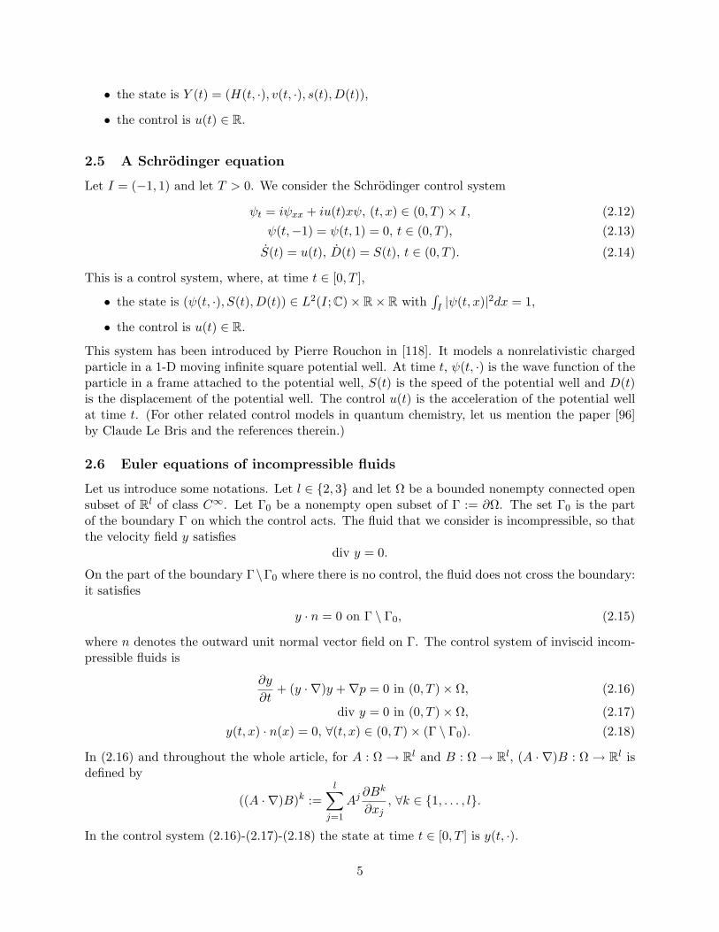
where (see Figure 1),
• L is the length of the 1-D tank,
• H (t, x) is the height of the fluid at time t and at the position x ∈ [0, L],
• v (t, x) is the horizontal water velocity of the fluid in a referential attached to the tank attime t and at the position x ∈ [0, L] (in the shallow water model, all the points on the samevertical have the same horizontal velocity),
• u (t) is the horizontal acceleration of the tank in the absolute referential,
• g is the gravity constant,
• s is the horizontal velocity of the tank,
• D is the horizontal displacement of the tank.
Local controllability of a 1-D tank containing auid modeled by the shallow-water equationJean-Michel CoronUniversité Paris-SudDépartement de Mathématique91405 Orsay, [email protected] April 2001H D x vL
1Figure 1: Fluid in the 1-D tank.
This is a control system where, at time t,
4
• the state is Y (t) = (H(t, ·), v(t, ·), s(t), D(t)),
• the control is u(t) ∈ R.
2.5 A Schrodinger equation
Let I = (−1, 1) and let T > 0. We consider the Schrodinger control system
ψt = iψxx + iu(t)xψ, (t, x) ∈ (0, T )× I, (2.12)ψ(t,−1) = ψ(t, 1) = 0, t ∈ (0, T ), (2.13)
S(t) = u(t), D(t) = S(t), t ∈ (0, T ). (2.14)
This is a control system, where, at time t ∈ [0, T ],
• the state is (ψ(t, ·), S(t), D(t)) ∈ L2(I; C)× R× R with∫I |ψ(t, x)|2dx = 1,
• the control is u(t) ∈ R.
This system has been introduced by Pierre Rouchon in [118]. It models a nonrelativistic chargedparticle in a 1-D moving infinite square potential well. At time t, ψ(t, ·) is the wave function of theparticle in a frame attached to the potential well, S(t) is the speed of the potential well and D(t)is the displacement of the potential well. The control u(t) is the acceleration of the potential wellat time t. (For other related control models in quantum chemistry, let us mention the paper [96]by Claude Le Bris and the references therein.)
2.6 Euler equations of incompressible fluids
Let us introduce some notations. Let l ∈ 2, 3 and let Ω be a bounded nonempty connected opensubset of Rl of class C∞. Let Γ0 be a nonempty open subset of Γ := ∂Ω. The set Γ0 is the partof the boundary Γ on which the control acts. The fluid that we consider is incompressible, so thatthe velocity field y satisfies
div y = 0.
On the part of the boundary Γ\Γ0 where there is no control, the fluid does not cross the boundary:it satisfies
y · n = 0 on Γ \ Γ0, (2.15)
where n denotes the outward unit normal vector field on Γ. The control system of inviscid incom-pressible fluids is
∂y
∂t+ (y · ∇)y +∇p = 0 in (0, T )× Ω, (2.16)
div y = 0 in (0, T )× Ω, (2.17)y(t, x) · n(x) = 0, ∀(t, x) ∈ (0, T )× (Γ \ Γ0). (2.18)
In (2.16) and throughout the whole article, for A : Ω → Rl and B : Ω → Rl, (A · ∇)B : Ω → Rl isdefined by
((A · ∇)B)k :=l∑
j=1
Aj∂Bk
∂xj, ∀k ∈ 1, . . . , l.
In the control system (2.16)-(2.17)-(2.18) the state at time t ∈ [0, T ] is y(t, ·).
5
Remark 1 In this formulation of the control system associated to the Euler equations, the controldoes not appear explicitly. One can take, for example, y · n on Γ with
∫Γ y · nds = 0 and
1. If l = 2, curl y on Γ for the incoming flow (i.e. at the points (t, x) ∈ [0, T ] × Γ such thaty(t, ·) · n(x) < 0)
2. If l = 3, the tangential component of curl y on Γ for the incoming flow.
2.7 Navier-Stokes of incompressible fluids
In this section the incompressible is now viscous. Equation (2.16) is replaced by
∂y
∂t− ν∆y + (y · ∇)y +∇p = 0 in (0, T )× Ω, (2.19)
where ν > 0 is the viscosity of the fluid (a positive real number independent of y: it depends only onthe considered incompressible fluid). Since (2.19) contains a spatial second order partial differentialterm (namely the Laplacian ∆y of y), the boundary condition (2.18) is no longer sufficient. Oneadd a “wall law”. Two wall laws are classical
• The Stokes noslip boundary condition:
y = 0 on (0, T )× (Γ \ Γ0), (2.20)
which implies (2.18).
• The Navier slip boundary condition: Besides (2.18), one also requires
σy · τ + (1− σ)i=l,j=l∑i=1,j=1
ni(∂yi
∂xj+∂yj
∂xi
)τ j = 0 on (0, T )× (Γ \ Γ0), ∀τ ∈ T Γ, (2.21)
where σ is a constant in [0, 1). In (2.21), n = (n1, . . . , nl), τ = (τ1, . . . , τ l) and T Γ is the setof tangent vector fields on the boundary Γ. Note that the Stokes boundary condition (2.20)corresponds to the case σ = 1
For the control, one can simply take u(t, x) :== y(t, x) for (t, x) ∈ (0, T )× (Γ \Γ0). Of course, dueto the smoothing effects of the Navier-Stokes equations, one cannot expect to move from a givenstate y0 to another given state y1 unless severe restrictions on the smoothness of y1, restrictionswhich are moreover not very explicit. In that case the good notion of controllability is the following:Given a state y0 and a solution (y, p) : [0, T ]×Ω → Rl ×R of the control system, does there existsa control u : [0, T ]×Γ0 → R such that the solution (y, p) : [0, T ]×Ω → Rl×R of the Navier-Stokescontrol system such that y(0, ·) = y0 satisfies y(T, ·) = y(T, ·)?
3 A general framework for control systems modeled by linearPDE’s
3.1 The framework
For two normed linear spaces H1 and H2, we denote by L(H1;H2) the set of continuous linear mapsfrom H1 into H2 and denote by ‖ · ‖L(H1;H2) the usual norm in this space.
6
Let H and U be two Hilbert spaces. Just to simplify the notations, these Hilbert spaces areassumed, in this section, to be real Hilbert spaces (the case of complex Hilbert spaces followsdirectly from the case of real Hilbert spaces). The space H is the state space and the space U isthe control space. We denote by (·, ·)H the scalar product in H, by (·, ·)U the scalar product in U ,by ‖ · ‖H the norm in H and by ‖ · ‖U the norm in U .
Let S(t), t ∈ [0,+∞), be a strongly continuous semigroup of continuous linear operators onH. Let A be the infinitesimal generator of the semigroup S(t), t ∈ [0,+∞). As usual, we denoteby S(t)∗ the adjoint of S(t). Then S(t)∗, t ∈ [0,+∞), is a strongly continuous semigroup ofcontinuous linear operators and the infinitesimal generator of this semigroup is the adjoint A∗ ofA. The domain D(A∗) is equipped with the usual graph norm ‖ · ‖D(A∗) of the unbounded operatorA∗:
‖z‖D(A∗) := ‖z‖H + ‖A∗z‖H , ∀z ∈ D(A∗).
This norm is associated to the scalar product in D(A∗) defined by
With this scalar product, D(A∗) is a Hilbert space. Let D(A∗)′ be the dual of D(A∗) with thepivot space H. In particular,
D(A∗) ⊂ H ⊂ D(A∗)′.
Let
B ∈ L(U,D(A∗)′). (3.1)
In other words, B is a linear map from U into the set of linear functions from D(A∗) into R suchthat, for some C > 0,
|(Bu)z| 6 C‖u‖U‖z‖D(A∗), ∀u ∈ U, ∀z ∈ D(A∗).
We also assume the following regularity property (also called admissibility condition):
∀T > 0,∃CT > 0 such that∫ T
0‖B∗S(t)∗z‖2
Udt 6 CT ‖z‖2H , ∀z ∈ D(A∗). (3.2)
In (3.2) and in the following, B∗ ∈ L(D(A∗);U) is the adjoint of B. It follows from (3.2) that theoperators (
z ∈ D(A∗))7→
((t 7→ B∗S(t)∗z) ∈ C0([0, T ];U)
),(
z ∈ D(A∗))7→
((t 7→ B∗S(T − t)∗z) ∈ C0([0, T ];U)
)can be extended in a unique way as continuous linear maps from H into L2((0, T );U). We use thesame symbols to denote these extensions.
Note that, using the fact that S(t)∗, t ∈ [0,+∞), is a strongly continuous semigroup of contin-uous linear operators on H, it is not hard to check that (3.2) is equivalent to
∃T > 0,∃CT > 0 such that∫ T
0‖B∗S(t)∗z‖2
Udt 6 CT ‖z‖2H , ∀z ∈ D(A∗).
The control system we consider here is
y = Ay +Bu, t ∈ (0, T ), (3.3)
7
where, at time t, the control is u(t) ∈ U and the state is y(t) ∈ H.Let T > 0, y0 ∈ H and u ∈ L2((0, T );U). We are interested in the Cauchy problem
y = Ay +Bu(t), t ∈ (0, T ), (3.4)
y(0) = y0. (3.5)
We first give the definition of a solution to (3.4)-(3.5). Let us first motivate our definition Letτ ∈ [0, T ] and ϕ : [0, τ ] → H. We take the scalar product in H of (3.4) with ϕ and integrate on[0, τ ]. At least formally, we get, using an integration by parts together with (3.5),
(y(τ), ϕ(τ))H − (y0, ϕ(0))H −∫ τ
0(y(t), ϕ(t) +A∗ϕ(t))Hdt =
∫ τ
0(u(t), B∗ϕ(t))Udt.
Taking ϕ(t) = S(τ − t)∗zτ , for every given zτ ∈ H, we have formally ϕ(t)+A∗φ(t) = 0, which leadsto the following definition.
Definition 2 Let T > 0, y0 ∈ H and u ∈ L2((0, T );U). A solution of the Cauchy problem (3.4)-(3.5) is a function y ∈ C0([0, T ];H) such that
(y(τ), zτ )H − (y0, S(τ)∗zτ )H =∫ τ
0(u(t), B∗S(τ − t)∗zτ )Udt, ∀τ ∈ [0, T ], ∀zτ ∈ H. (3.6)
Note that, by the regularity property (3.2), the right hand side of (3.6) is well defined (see page 7).With this definition one has the following theorem.
Theorem 3 Let T > 0. Then, for every y0 ∈ H and for every u ∈ L2((0, T );U), the Cauchyproblem (3.4)-(3.5) has a unique solution y. Moreover, there exists C = C(T ) > 0, independent ofy0 ∈ H and u ∈ L2((0, T );U), such that
For a proof of this theorem, see, for example [38, pages 53–54].
3.2 Examples
In this section, we show how to put the linear control systems of Section 2 in the above generalframework.
3.2.1 A transport equation
We return to the control system (2.1)-(2.2). Let L > 0. The linear control system we study is
yt + yx = 0, t ∈ (0, T ), x ∈ (0, L), (3.8)y(t, 0) = u(t), t ∈ (0, T ), (3.9)
where, at time t, the control is u(t) ∈ R and the state is y(t, ·) : (0, L) → R.For the Hilbert space H, we take H := L2(0, L). For the operator A : D(A) → H we take
As the operator A, the operator A∗ is also dissipative. Hence, by the Lumer-Phillips theorem, theoperator A is the infinitesimal generator of a strongly continuous semigroup S(t), t ∈ [0,+∞), ofcontinuous linear operators on H.
For the Hilbert space U , we take U := R. The operator B : R → D(A∗)′ is defined by
(Bu)z = uz(0), ∀u ∈ R,∀z ∈ D(A∗). (3.10)
Note that B∗ : D(A∗) → R is defined by
B∗z = z(0), ∀z ∈ D(A∗).
Let us deal with the regularity property (3.2). Let z0 ∈ D(A∗). Let
z ∈ C0([0, T ];D(A∗)) ∩ C1([0, T ];L2(0, L))
be defined by z(t, ·) = S(t)∗z0. Inequality (3.2) is equivalent to∫ T
0z(t, 0)2dt 6 CT
∫ L
0z0(x)2dx. (3.11)
Let us prove this inequality for CT := 1. We have
zt = zx, t ∈ (0, T ), x ∈ (0, L), (3.12)z(t, L) = 0, t ∈ (0, T ), (3.13)
z(0, x) = z0(x), x ∈ (0, L). (3.14)
We multiply (3.12) by z and integrate on [0, T ] × [0, L]. Using (3.13), (3.14) and integrations byparts, we get ∫ T
0z(t, 0)2dt =
∫ L
0z0(x)2dx−
∫ L
0z(T, x)2dx 6
∫ L
0z0(x)2dx, (3.15)
which shows that (3.11) holds for CT := 1.In fact, as one can easily check, the solution to the following Cauchy problem (in the senses of
Definition 2)
yt + yx = 0, t ∈ (0, T ), x ∈ (0, L), (3.16)y(t, 0) = u(t), t ∈ (0, T ), (3.17)
y(0, x) = y0(x), x ∈ (0, L), (3.18)
where T > 0, y0 ∈ L2(0, L) and u ∈ L2(0, T ) are given data, is
y(t, x) = y0(x− t), ∀(t, x) ∈ [0, T ]× (0, L) such that t 6 x, (3.19)y(t, x) = u(t− x), ∀(t, x) ∈ [0, T ]× (0, L) such that t > x. (3.20)
9
3.2.2 A linear Korteweg-de Vries equation
We return to the linear Korteweg-de Vries equation already mentioned in Section 2. Let L > 0.The linear control system we study is
yt + yx + yxxx = 0, t ∈ (0, T ), x ∈ (0, L), (3.21)y(t, 0) = y(t, L) = 0, yx(t, L) = u(t), t ∈ (0, T ), (3.22)
where, at time t, the control is u(t) ∈ R and the state is y(t, ·) : (0, L) → R.For the Hilbert space H, we take H = L2(0, L). For the operator A : D(A) → H, we take
Then D(A) is dense in L2(0, L), A is closed. Simple integrations by parts give
(Af, f)L2(0,L) = −12fx(0)2, ∀f ∈ L2(0, L),
which shows that A is dissipative. The adjoint A∗ of A is defined by
D(A∗) := f ∈ H3(0, L); f(0) = f(L) = fx(0) = 0,A∗f := fx + fxxx, ∀f ∈ D(A∗).
As A, the operator A∗ is also dissipative. Hence, by the Lumer-Phillips theorem, the operator Ais the infinitesimal generator of a strongly continuous semigroup S(t), t ∈ [0,+∞), of continuouslinear operators on L2(0, L).
For the Hilbert space U , we take U := R. The operator B : R → D(A∗)′ is defined by
(Bu)z = uzx(L), ∀u ∈ R,∀z ∈ D(A∗). (3.23)
Note that B∗ : D(A∗) → R is defined by
B∗z = zx(L), ∀z ∈ D(A∗).
Let us check the regularity property (3.2). Let z0 ∈ D(A∗). Let
We multiply (3.26) by z and integrate on (0, T )×(0, L). Using (3.27), (3.28) and simple integrationsby parts one gets∫ T
0|zx(t, L)|2dt =
∫ L
0|z0(x)|2dx−
∫ L
0|z(T, x)|2dx 6
∫ L
0|z0(x)|2dx, (3.29)
which shows that (3.25) holds with CT := 1.
10
3.2.3 A heat equation
We return to the linear heat equation already considered in Section 2. Let Ω be a non empty opensubset of Rl and let ω be a non empty open subset of Ω. The linear heat equation considered inthis section is
yt −∆y = u(t, x), t ∈ (0, T ), x ∈ Ω, (3.30)y = 0 on (0, T )× ∂Ω, (3.31)
where, at time t ∈ [0, T ], the state is y(t, ·) ∈ L2(Ω) and the control is u(t, ·) ∈ L2(Ω). We requirethat
u(·, x) = 0, x ∈ Ω \ ω. (3.32)
One can put this linear control system in the general framework detailed in Section 3 in the followingway. One chooses
H := L2(Ω),
equipped with the usual scalar product. Let A : D(A) ⊂ H → H be the linear operator defined by
D(A) :=y ∈ H1
0 (Ω); ∆y ∈ L2(Ω),
Ay := ∆y ∈ H.
Note that, if Ω is smooth enough (for example of class C2), then
D(A) = H10 (Ω) ∩H2(Ω). (3.33)
However, without any regularity assumption on Ω, (3.33) is wrong in general (see in particular [66,Theorem 2.4.3, page 57] by Pierre Grisvard). One easily checks that
D(A) is dense in L2(Ω), (3.34)A is closed. (3.35)
Moreover,
(Ay, y)H = −∫
Ω|∇y|2dx, ∀y ∈ D(A). (3.36)
Let A∗ be the adjoint of A. One easily checks that
A∗ = A. (3.37)
From the Lumer-Phillips theorem, (3.34), (3.35), (3.36) and (3.37), A is the infinitesimal generatorof a strongly continuous semigroup of linear contractions S(t), t ∈ [0,+∞), on H. For the Hilbertspace U we take L2(ω). The linear map B ∈ L(U ;D(A∗)′) is the map which is defined by
(Bu)ϕ =∫ωuϕdx.
Note that B ∈ L(U ;H). Hence the regularity property (3.2) is automatically satisfied.
11
4 Controllability of linear control systems
4.1 Different types of controllability
In this section we are interested in the controllability of the control system (3.3). In contrast tothe case of linear finite-dimensional control systems, many types of controllability are possible andinteresting. We define here three types of controllability.
Definition 4 Let T > 0. The control system (3.3) is exactly controllable in time T if, for everyy0 ∈ H and for every y1 ∈ H, there exists u ∈ L2((0, T );U) such that the solution y of the Cauchyproblem
y = Ay +Bu(t), y(0) = y0, (4.1)
satisfies y(T ) = y1.
Definition 5 Let T > 0. The control system (3.3) is null controllable in time T if, for everyy0 ∈ H and for every y0 ∈ H, there exists u ∈ L2((0, T );U) such that the solution of the Cauchyproblem (4.1) satisfies y(T ) = S(T )y0.
Let us point out that, by linearity, we get an equivalent definition of “null controllable in time T” if,in Definition 5, one assumes that y0 = 0. This explains the usual terminology “null controllability”.
Definition 6 Let T > 0. The control system (3.3) is approximately controllable in time T if, forevery y0 ∈ H, for every y1 ∈ H, and for every ε > 0, there exists u ∈ L2((0, T );U) such that thesolution y of the Cauchy problem (4.1) satisfies ‖y(T )− y1‖H 6 ε.
Clearly
(exact controllability) ⇒ (null controllability and approximate controllability).
The converse is false in general (see, for example, the control system (3.30)-(3.31) below). However,the converse holds if S is a strongly continuous group of linear operators. More precisely, one hasthe following theorem.
Theorem 7 Assume that S(t), t ∈ R, is a strongly continuous group of linear operators. LetT > 0. Assume that the control system (3.3) is null controllable in time T . Then the controlsystem (3.3) is exactly controllable in time T .
Proof of Theorem 7. Let y0 ∈ H and y1 ∈ H. From the null controllability assumption appliedto the initial data y0 − S(−T )y1, there exists u ∈ L2((0, T );U) such that the solution y of theCauchy problem
˙y = Ay +Bu(t), y(0) = y0 − S(−T )y1,
satisfies
y(T ) = 0. (4.2)
One easily sees that the solution y of the Cauchy problem
y = Ay +Bu(t), y(0) = y0,
12
is given by
y(t) = y(t) + S(t− T )y1, ∀t ∈ [0, T ]. (4.3)
In particular, from (4.2) and (4.3),y(T ) = y1.
This concludes the proof of Theorem 7.
4.2 Methods to study controllability
Rouhgly speaking there are essentially two types of methods to study the controllability of linearPDE, namely direct methods and duality methods.
4.2.1 Direct methods
Among these methods, let us mention in particular
• The extension method. See, for example, [121] and [122, Proof of Theorem 5.3, pages 688–690]by David Russell, [105] by Walter Littman and [38, Section 2.1.2.2, pages 30-34].
• Moment theory. See, for example, [89] by Werner Krabs, [88] by Vilmos Komornik and PaolaLoreti, [7] by Sergei Avdonin and Sergei Ivanov, and [38, Section 2.6, pages 95-99]. We givean example of an application of the moment theory for a Schrodinger equation in Section4.3.2.
• Flatness. This approach has been initiated in the framework of control theory in finitedimension by Michel Fliess, Jean Levine, Pierre Rouchon and Philippe Martin in [56]. Forapplications of this method for the control of linear PDE, see, in particular, [108] by HuguesMounier, Joachim Rudolph, Michel Fliess and Pierre Rouchon,, [91] by Beatrice Laroche,Philippe Martin and Pierre Rouchon, [110] by Nicolas Petit and Pierre Rouchon, as well asthe article by Pierre Rouchon in Scholarpedia.
4.2.2 Duality methods
Let us now introduce some “optimal control maps”. Let us first deal with the case where the controlsystem (3.3) is exactly controllable in time T . Then, for every y1, the set UT (y1) of u ∈ L2((0, T );U)such that
(y = Ay +Bu(t), y(0) = 0) ⇒ (y(T ) = y1)
is nonempty. Clearly the set UT (y1) is a closed affine subspace of L2((0, T );U). Let us denote byUT (y1) the projection of 0 on this closed affine subspace, i.e., the element of UT (y1) of the smallestL2((0, T );U)-norm. Then it is not hard to see that the map
UT : H → L2((0, T );U)y1 7→ UT (y1)
is a linear map. Moreover, using the closed graph theorem (see, for example, [119, Theorem 2.15,page 50]) one readily checks that this linear map is continuous.
13
Let us now deal with the case where the control system (3.3) is null controllable in time T .Then, for every y0, the set UT (y0) of u ∈ L2((0, T );U) such that
(y = Ay +Bu(t), y(0) = y0) ⇒ (y(T ) = 0)
is nonempty. Clearly the set UT (y0) is a closed affine subspace of L2((0, T );U). Let us denote byUT (y0) the projection of 0 on this closed affine subspace, i.e., the element of UT (y0) of the smallestL2((0, T );U)-norm. Then, again, it is not hard to see that the map
UT : H → L2((0, T );U)y0 7→ UT (y0)
is a continuous linear map.The main results of this section are the following ones.
Theorem 8 Let T > 0. The control system (3.3) is exactly controllable in time T if and only ifthere exists c > 0 such that ∫ T
0‖B∗S(t)∗z‖2
Udt > c‖z‖2H , ∀z ∈ D(A∗). (4.4)
Moreover, if such a c > 0 exists and if cT is the maximum of the set of c > 0 such that (4.4) holds,one has ∥∥UT∥∥
L(H;L2((0,T );U))=
1√cT. (4.5)
Theorem 9 The control system (3.3) is approximately controllable in time T if and only if, forevery z ∈ H,
(B∗S(·)∗z = 0 in L2((0, T );U)) ⇒ (z = 0). (4.6)
Theorem 10 Let T > 0. The control system (3.3) is null controllable in time T if and only ifthere exists c > 0 such that∫ T
0‖B∗S(t)∗z‖2
Udt > c‖S(T )∗z‖2H , ∀z ∈ D(A∗). (4.7)
Moreover, if such a c > 0 exists and if cT is the maximum of the set of c > 0 such that (4.7) holds,then
‖UT ‖L(H;L2((0,T );U)) =1√cT. (4.8)
Theorem 11 Assume that, for every T > 0, the control system (3.3) is null controllable in timeT . Then, for every T > 0, the control system (3.3) is approximately controllable in time T .
For a proof of these theorems, see, for example [38, Section 2.3.2]. Inequalities (4.4) and (4.7) areusually called observability inequalities for the abstract linear control system y = Ay + Bu. Thedifficulty is to prove them! For this purpose, there are many methods available (but still manyopen problems). Among these methods, let us mention in particular
14
• Multiplier methods. See in particular, [103] by Jacques-Louis Lions, [86] by Vilmos Komornik,[139] by Enrique Zuazua. For a simple example of this method, see Section 4.3.1.
• Microlocal analysis. See in particular [12] by Claude Bardos, Gilles Lebeau and Jeffrey Rauchand the appendix 2 of the book [103].
Remark 12 In contrast to Theorem 11, note that, for a given T > 0, the null controllability intime T does not imply the approximate controllability in time T . For example, let L > 0 and let ustake H := L2(0, L) and U := 0. We consider the linear control system
yt + yx = 0, t ∈ (0, T ), x ∈ (0, L), (4.9)y(t, 0) = u(t) = 0, t ∈ (0, T ). (4.10)
In Section 4.3.1, we shall see how to put this control system in the abstract framework y = Ay+Bu.It follows from (3.20), that, whatever y0 ∈ L2(0, L) is, the solution to the Cauchy problem (seeDefinition 2)
yt + yx = 0, t ∈ (0, T ), x ∈ (0, L),y(t, 0) = u(t) = 0, t ∈ (0, T ),
y(0, x) = y0(x), x ∈ (0, L),
satisfiesy(T, ·) = 0, if T > L.
In particular, if T > L, the linear control system (4.9)-(4.10) is null controllable but is not approx-imately controllable.
4.3 Examples
4.3.1 A transport equation
We return to the transport control system (3.8)-(3.9). This example is pedagogically interestingsince one can give explicitly the solution to the Cauchy problem (3.16)-(3.17)-(3.18) where T > 0,y0 ∈ L2(0, L) and u ∈ L2(0, T ) are given. This solution is given by (3.19)-(3.20). From this explicitsolution one readily gets
Proposition 13 The control system (3.8)-(3.9) is
• exactly controllable in time T if and only if T > L,
• null controllable in time T if and only if T > L,
• approximately controllable in time T if and only if T > L.
Let us show how to use the multiplier method in order to prove that if
T > L (4.11)
then the control system (3.8)-(3.9) is exactly controllable. By Theorem 8, the exact controllabilityin time T is equivalent to the existence of c > 0 such that∫ T
0z(t, 0)2dt > c
∫ L
0z0(x)2dx, (4.12)
15
where z : [0, T ]× [0, L] → R is the solution of the Cauchy problem
zt − zx = 0, (4.13)z(t, L) = 0, t ∈ (0, T ), (4.14)
z(0, ·) = z0. (4.15)
Let us prove prove (4.12). With simple density arguments, we may assume that z is of class C1. Letus multiply (4.13) by the mutiplier z and integrate the obtained equality on [0, L]. Using (4.14),one gets
ddt
(∫ L
0|z(t, x)|2dx
)= −|z(t, 0)|2. (4.16)
Let us now multiply (4.13) by the mutiplier xz and integrate the obtained equality on [0, L]. Using(4.14), one gets
ddt
(∫ L
0x|z(t, x)|2dx
)= −
∫ L
0|z(t, x)|2dx. (4.17)
For t ∈ [0, T ], let e(t) :=∫ L0 |z(t, x)|2dx. From (4.17), we have∫ T
0e(t)dt = −
∫ L
0x|z(T, x)|2dx+
∫ L
0x|z(0, x)|2dx
6 L
∫ L
0|z(0, x)|2dx = Le(0). (4.18)
From (4.16), we get
e(t) = e(0)−∫ t
0|z(τ, 0)|2dτ > e(0)−
∫ T
0|z(τ, 0)|2dτ. (4.19)
From (4.15), (4.18) and (4.19), we get
(T − L)‖z0‖2L2(0,L) 6 T
∫ T
0|z(τ, 0)|2dτ, (4.20)
which proves the observability inequality (4.12) with c given by
c :=
√T − L
T. (4.21)
4.3.2 A linear Schrodinger equation
We return to the nonlinear Schrodinger control system consider in Section 2.5. For simplicity, weforget the variables S and D: the control system is simply (2.12)-(2.13). In this section how themoment methods can be used in order to prove the controllability of linearized control systemaround important trajectories of the control system (2.12)-(2.13).
Let I be the open interval (−1, 1). For γ ∈ R, let Aγ : D(Aγ) ⊂ L2(I; C) → L2(I; C) be theoperator defined on
D(Aγ) := H2(I; C) ∩H10 (I; C) (4.22)
16
by
Aγϕ := −ϕxx − γxϕ. (4.23)
In (4.22), as usual,H1
0 (I; C) := ϕ ∈ H1((0, L); C); ϕ(0) = ϕ(L) = 0.
We denote by 〈·, ·〉 the usual Hermitian scalar product in the Hilbert space L2(I; C):
〈ϕ,ψ〉 :=∫Iϕ(x)ψ(x)dx, (4.24)
where z denotes the complex conjugate of the complex number z. Note that
D(Aγ) is dense in L2(I; C), (4.25)Aγ is closed, (4.26)
A∗γ = Aγ , (i.e., Aγ is self-adjoint), (4.27)
Aγ has compact resolvent. (4.28)
Let us recall that (4.28) means that there exists a real α in the resolvent set of Aγ such that theoperator (αId− Aγ)−1 is compact from L2(I; C) into L2(I; C), where Id denotes the identity mapon H (see, for example, [84, pages 36 and 187]). Then (see, for example, [84, page 277]), the Hilbertspace L2(I; C) has a complete orthonormal system (ϕk,γ)k∈N\0 of eigenfunctions for the operatorAγ :
Aγϕk,γ = λk,γϕk,γ ,
where (λk,γ)k∈N\0 is an increasing sequence of positive real numbers. Let S be the unit sphere ofL2(I; C):
S := φ ∈ L2(I; C);∫I|φ(x)|2dx = 1 (4.29)
and, for φ ∈ S, let TSφ be the tangent space to S at φ:
TSφ := Φ ∈ L2(I; C); <〈Φ, φ〉 = 0, (4.30)
where, as usual, <z denotes the real part of the complex number z. Let
ψ1,γ(t, x) := e−iλ1,γtϕ1,γ(x), (t, x) ∈ (0, T )× I. (4.31)
Note that
ψ1,γt = iψ1,γxx + iγxψ1,γ , t ∈ (0, T ), x ∈ I,ψ1,γ(t,−1) = ψ1,γ(t, 1) = 0, t ∈ (0, T ),∫
I|ψ1,γ(t, x)|2dx = 1, t ∈ (0, T ).
Hence (ψ, u) = (ψ1,γ , γ) is a trajectory of the control system (2.12)-(2.13). The linearized controlsystem around this trajectory is the following linear control system:
Ψt = iΨxx + iγxΨ + iuxψ1,γ , (t, x) ∈ (0, T )× I, (4.32)Ψ(t,−1) = Ψ(t, 1) = 0, t ∈ (0, T ). (4.33)
This is a control system where, at time t ∈ [0, T ],
17
• The state is Ψ(t, ·) ∈ L2(I; C) with Ψ(t, ·) ∈ TS(ψ1,γ(t, ·)).
• The control is u(t) ∈ R.
Let us first deal with the Cauchy problem
Ψt = iΨxx + iγxΨ + iuxψ1,γ , (t, x) ∈ (0, T )× I, (4.34)Ψ(t,−1) = Ψ(t, 1) = 0, t ∈ (0, T ), (4.35)
Ψ(0, x) = Ψ0(x), (4.36)
where T > 0, u ∈ L1(0, T ) and Ψ0 ∈ L2(I; C) are given. By (4.27),
(−iAγ)∗ = −(−iAγ).
Therefore, by the Lumer-Phillips theorem −iAγ is the infinitesimal generator of a strongly contin-uous group of linear isometries on L2(I; C). We denote by Sγ(t), t ∈ R, this group.
Note that, since ψ1,γ depends on time, Section 3.1 cannot be applied. Our notion of solution tothe Cauchy problem (4.34)-(4.35)-(4.36) is given in the following definition.
Definition 14 Let T > 0, u ∈ L1(0, T ) and Ψ0 ∈ L2(I; C). A solution Ψ : [0, T ] × I → C to theCauchy problem (4.34)-(4.35)-(4.36) is the function Ψ ∈ C0([0, T ];L2(I; C)) defined by
Ψ(t) = Sγ(t)Ψ0 +∫ t
0Sγ(t− τ)iu(τ)xψ1,γ(τ, ·)dτ. (4.37)
With this definition and standard arguments, one can show that the Cauchy problem (4.34)-(4.35)-(4.36) is well posed (see e.g. [38, Theorem A.7, page 375]).
Let us now study the controllability of the linear Schrodinger control system (4.32)-(4.33). Let
The goal of this section is to prove the following controllability result due to Karine Beauchard [13,Theorem 5, page 862].
Theorem 15 There exists γ0 > 0 such that, for every T > 0, for every γ ∈ (0, γ0], for everyΨ0 ∈ TSψ1,γ(0, ·)∩H3
(0)(I; C) and for every Ψ1 ∈ TSψ1,γ(T, ·)∩H3(0)(I; C), there exists u ∈ L2(0, T )
such that the solution of the Cauchy problem
Ψt = iΨxx + iγxΨ + iu(t)xψ1,γ , t ∈ (0, T ), x ∈ I, (4.39)Ψ(t,−1) = Ψ(t, 1) = 0, t ∈ (0, T ), (4.40)
Ψ(0, x) = Ψ0(x), x ∈ I, (4.41)
satisfies
Ψ(T, x) = Ψ1(x), x ∈ I. (4.42)
We are also going to see that the conclusion of Theorem 15 does not hold for γ = 0 (as alreadynoted by Pierre Rouchon in [118]).
Proof of Theorem 15. Let T > 0,
Ψ0 ∈ TS(ψ1,γ(0, ·)) and Ψ1 ∈ TS(ψ1,γ(T, ·)).
18
Let u ∈ L2(0, T ). Let Ψ be the solution of the Cauchy problem (4.39)-(4.40)-(4.41). Let us decom-pose Ψ(t, ·) in the complete orthonormal system (ϕk,γ)k∈N\0 of eigenfunctions for the operatorAγ :
Ψ(t, ·) =∞∑k=1
yk(t)ϕk,γ .
Taking the Hermitian product of (4.39) with ϕk,γ , one readily gets, using (4.40) and integrationsby parts,
yk = −iλk,γyk + ibk,γu(t)e−iλ1,γt, (4.43)
with
bk,γ := 〈ϕk,γ , xϕ1,γ〉 ∈ R. (4.44)
Note that (4.41) is equivalent to
yk(0) = 〈Ψ0, ϕk,γ〉, ∀k ∈ N \ 0. (4.45)
From (4.44) and (4.45) one gets
yk(T ) = e−iλk,γT (〈Ψ0, ϕk,γ〉+ ibk,γ
∫ T
0u(t)ei(λk,γ−λ1,γ)tdt). (4.46)
By (4.46), (4.42) is equivalent to the following so-called moment problem on u:
bk,γ
∫ T
0u(t)ei(λk,γ−λ1,γ)tdt = i
(〈Ψ0, ϕk,γ〉 − 〈Ψ1, ϕk,γ〉eiλk,γT
),∀k ∈ N \ 0. (4.47)
Let us now explain why for γ = 0 the conclusion of Theorem 15 does not hold. Indeed, one has
ϕn,0(x) := sin(nπx/2), n ∈ N \ 0, if n is even, (4.48)ϕn,0(x) := cos(nπx/2), n ∈ N \ 0, if n is odd. (4.49)
In particular, xϕ1,0ϕk,0 is an odd function if k is odd. Therefore
bk,0 = 0 if k is odd.
Hence, by (4.47), if there exists k odd such that
〈Ψ0, ϕk,0〉 − 〈Ψ1, ϕk,0〉eiλk,0T 6= 0,
there is no control u ∈ L2(0, T ) such that the solution of the Cauchy problem (4.39)-(4.40)-(4.41)(with γ = 0) satisfies (4.42).
Let us now turn to the case where γ is small but not 0. Since Ψ0 is in TS(ψ1,γ(0, ·)),
<〈Ψ0, ϕ1,γ〉 = 0. (4.50)
Similarly, the fact that Ψ1 is in TS(ψ1,γ(T, ·)) tells us that
<(〈Ψ1, ϕ1,γ〉eiλ1,γT ) = 0. (4.51)
The key ingredient to prove Theorem 15 is the following theorem.
19
Theorem 16 Let (µi)i∈N\0 be a sequence of real numbers such that
µ1 = 0, (4.52)there exists ρ > 0 such that µi+1 − µi > ρ, ∀i ∈ N \ 0. (4.53)
Let T > 0 be such that
limx→+∞
N(x)x
<T
2π, (4.54)
where, for every x > 0, N(x) is the largest number of µj’s contained in an interval of length x.Then there exists C > 0 such that, for every sequence (ck)k∈N\0 of complex numbers such that
c1 ∈ R, (4.55)∞∑k=1
|ck|2 <∞, (4.56)
there exists a (real-valued) function u ∈ L2(0, T ) such that∫ T
0u(t)eiµktdt = ck, ∀k ∈ N \ 0, (4.57)∫ T
0u(t)2dt 6 C
∞∑k=1
|ck|2. (4.58)
Remark 17 Theorem 16 is due do Jean-Pierre Kahane [83, Theorem III.6.1, page 114]; see also[20, pages 341–365] by Arne Beurling. See also, in the context of control theory, [120, Section 3]by David Russell who uses prior works [77] by Albert Ingham, [115] by Ray Redheffer and [124]by Laurent Schwartz. For a proof of Theorem 16, see, for example, [89, Section 1.2.2] by WernerKrabs, [88, Chapter 9] by Vilmos Komornik and Paola Loreti or [7, Chapter II, Section 4] by SergeiAvdonin and Sergei Ivanov. Improvements of Theorem 16 have been obtained by Stephane Jaffard,Marius Tucsnak and Enrique Zuazua in [81, 82], by Stephane Jaffard and Sorin Micu in [80], byClaudio Baiocchi, Vilmos Komornik and Paola Loreti in [8] and by Vilmos Komornik and PaolaLoreti in [87] and in [88, Theorem 9.4, page 177].
Note that, by (4.50) and (4.51),
i(〈Ψ0, ϕ1,γ〉 − 〈Ψ1, ϕ1,γ〉eiλ1,γT ) ∈ R. (4.59)
Hence, in order to apply Theorem 15 to our moment problem, it remains to estimate λk,γ and bk,γ .This is done in the following propositions, due to Karine Beauchard.
Proposition 18 ([13, Proposition 41, pages 937–938]) There exist γ0 > 0 and C0 > 0 suchthat, for every γ ∈ [−γ0, γ0] and for every k ∈ N \ 0,∣∣∣∣λk,γ − π2k2
4
∣∣∣∣ 6 C0γ2
k.
20
Proposition 19 ([13, Proposition 1, page 860]) There exist γ1 > 0 and C > 0 such that, forevery γ ∈ (0, γ1] and for every even integer k > 2,∣∣∣∣∣bk,γ − (−1)
k2+18k
π2(k2 − 1)2
∣∣∣∣∣ < Cγ
k3,
and for every odd integer k > 3,∣∣∣∣∣bk,γ − γ2(−1)
k−12 (k2 + 1)
π4k(k2 − 1)2
∣∣∣∣∣ < Cγ2
k3.
It is a classical result that
ϕ :=+∞∑k=1
dkϕk,γ ∈ H3(0)(I; C)
if and only if+∞∑k=1
k6|dk|2 < +∞.
Hence, Theorem 15 readily follows from Theorem 16 applied to the moment problem (4.47) withthe help of Proposition 18 and Proposition 19.
Remark 20 The moment method does not work well for the Schrodinger in dimension larger than1 (see, however, [79] by Stephane Jaffard in dimension 2). For these dimensions controllabilityresults have been obtained by means of other methods. Let us mention, in particular,
• The use of the multipliers method. See, in particular, [93] by Irena Lasiecka and RobertoTriggiani, [48] by Caroline Fabre, [106] by Elaine Machtyngier, [107] by Elaine Machtyngierand Enrique Zuazua.
• The use of microlocal analysis. See, in particular, [97] by Gilles Lebeau and [111] by Kim-Dang Phung, which rely use of the exact controllability result [12] by Claude Bardos, GillesLebeau and Jeffrey Rauch for the wave equation. See also [25] by Nicolas Burq.
For a survey on these results, see, in particular, [136] by Enrique Zuazua.
4.3.3 A linear Korteweg-de Vries equation
We go back to the linear Korteweg-de Vries equation control system (3.21)-(3.22) already consideredin Section 3.2.2. Let
N :=
2π
√j2 + l2 + jl
3; j, l ∈ N \ 0
. (4.60)
Then one has the following theorem, due to Lionel Rosier [116],
Theorem 21 Let T > 0. The control system (3.21)-(3.22) is exactly controllable in time T if andonly if L 6∈ N . Moreover, if L ∈ N , then the control system (3.21)-(3.22) is neither approximatelycontrollable nor null controllable in time T .
21
For a proof of Theorem 21, see [116] or [38, Section 2.2.2, pages 42-48]. Let us only point out that2π ∈ N (take j = l = 1 in (4.60) and that for L = 2π and for every T > 0 the control system(3.21)-(3.22) is neither approximately controllable nor null controllable in time T . This readilyfollows from the following observation. Let T > 0, let y0 ∈ L2(0, L), and let u ∈ L2(0, L). Lety ∈ C0([0, T ];L2(0, L)) be the solution to the Cauchy problem (see Definition 2)
yt + yx + yxxx = 0, t ∈ (0, T ), x ∈ (0, 2π), (4.61)y(t, 0) = y(t, L) = 0, yx(t, L) = u(t), t ∈ (0, T ), (4.62)
y(0, x) = y0(x), x ∈ (0, 2π). (4.63)
We multiply (4.61) by (1−cos(x)) and integrate on (0, 2π). Using (4.62) together with integrationsby parts, one gets (first when y is smooth enough and by density for the general case)
d
dt
∫ 2π
0(1− cos(x))ydx = 0,
which shows that the control system (3.21)-(3.22) is neither approximately controllable nor nullcontrollable in time T .
4.3.4 A heat equation
We go back to the control system (3.30)-(3.31)-(3.32) and show how Carleman allows to prove thefollowing theorem, due to Hector Fattorini and David Russell [53, Theorem 3.3] if n = 1, to OlegImanuvilov [73, 74] (see also the book [59] by Andrei Fursikov and Oleg Imanuvilov) and to GillesLebeau and Luc Robbiano [98] for n > 1.
Theorem 22 Let us assume that Ω is of class C2 and connected. Then, for every T > 0 the controlsystem (3.30)-(3.31)-(3.32) is null controllable and approximately controllable in time T .
Sketch of the proof of Theorem 22. Let T > 0. With the notations of Section 3.2.3, fory0 ∈ L2(Ω),
(B∗S∗(t)y0)(x) = y(t, x), t ∈ (0, T ), x ∈ ω, (4.64)
where y : (0,+∞)× Ω → R is defined by
yt −∆y = 0, (t, x) ∈ (0, T )× Ω, (4.65)y = 0 on (0, T )× ∂Ω, (4.66)
y(0, x) = y0(x), x ∈ Ω, (4.67)
The first step is the following lemma, due to Oleg Imanuvilov [74, Lemma 1.2] (see also [59,Lemma 1.1 page 4] and [38, Lemma 2.68 page 80]) and whose proof is omitted.
Lemma 23 There exists ψ ∈ C2(Ω) such that
ψ > 0 in Ω, ψ = 0 on ∂Ω, (4.68)
|∇ψ(x)| > 0, ∀x ∈ Ω \ ω0. (4.69)
Remark 24 In the case n = 1, Ω = (a, b) for some real numbers a < b. Let us take c ∈ ω. Thenψ : Ω → R defined by
ψ(x) := (b− c)3 − (x− c)3, if x ∈ [c, b], ψ(x) := (c− a)3 − (c− x)3, if x ∈ [a, c],
satisfies (4.68)-(4.69).
22
Let us fix ψ as in Lemma 23. Let α : (0, T ) × Ω → (0,+∞) and φ : (0, T ) × Ω → (0,+∞) bedefined by
α(t, x) =e2λ‖ψ‖C0(Ω) − eλψ(x)
t(T − t), ∀(t, x) ∈ (0, T )× Ω, (4.70)
φ(t, x) =eλψ(x)
t(T − t), ∀(t, x) ∈ (0, T )× Ω, (4.71)
where λ ∈ [1,+∞) will be chosen later on. Let z : [0, T ]× Ω → R be defined by
where s ∈ [1,+∞) will be chosen later on. From (4.65), (4.70), (4.71) and (4.72), we have
P1 + P2 = P3 (4.74)
with
P1 := −∆z − s2λ2φ2|∇ψ|2z + sαtz, (4.75)
P2 := zt + 2sλφ∇ψ∇z + 2sλ2φ|∇ψ|2z, (4.76)
P3 := −sλφ(∆ψ)z + sλ2φ|∇ψ|2z. (4.77)
Let Q := (0, T )× Ω. From (4.74), we have
2∫ ∫
QP1P2dxdt 6
∫ ∫QP 2
3 dxdt. (4.78)
Let n denote the outward unit normal vector field on ∂Ω. Note that z vanishes on [0, T ] × ∂Ω(see (4.66) and (4.72)) and on 0, T × Ω (see (4.73)). Then straightforward computations usingintegrations by parts lead to
In (4.81) and until the end of the proof of Theorem 22, we use the usual repeated-index sumconvention. By (4.69) and (4.71), there exists Λ such that, for every λ > Λ, we have, on (0, T ) ×(Ω \ ω0),
Using (4.78) to (4.88), we get the existence of C > 0 such that, for every s > 1 and for every y0,
s3∫
(0,T )
∫Ω\ω0
|z|2
t3(T − t)3dxdt 6 Cs2
∫ ∫Q
|z|2
t3(T − t)3dxdt+ Cs3
∫(0,T )
∫ω0
|∇z|2 + |z|2
t3(T − t)3dxdt.
(4.89)
Taking for s > 1 large enough in (4.89), one gets
s3∫
(0,T )
∫Ω\ω0
|z|2
t3(T − t)3dxdt 6 Cs3
∫(0,T )
∫ω0
|∇z|2 + |z|2
t3(T − t)3dxdt. (4.90)
From Theorem 9, (4.72), and (4.90), one gets the approximate controllability in time T (withH := L2(Ω) and U := L2(ω); see Definition 6) of the control system (3.30)-(3.31)-(3.32).
Let us now deal with the null controllability. Taking s > 1 large enough in (4.89), one gets theexistence of c0 > 0 independent of y0 such that∫ 2T/3
T/3
∫Ω|z|2dxdt 6 c0
∫ T
0
∫ω0
|∇z|2 + |z|2
t3(T − t)3dxdt. (4.91)
We choose such an s and such a c0. Coming back to y using (4.70) and (4.72), we deduce from(4.91) the existence of c1 > 0 independent of y0 such that∫ 2T/3
T/3
∫Ω|y|2dxdt 6 c1
∫ T
0
∫ω0
t(T − t)(|∇y|2 + |y|2)dxdt. (4.92)
Let ρ ∈ C∞(Ω) be such that
ρ = 1 in ω0,
ρ = 0 in Ω \ ω.
24
We multiply (4.65) by t(T − t)ρy and integrate on Q. Using (4.66) and integrations by parts, weget the existence of c2 > 0 independent of y0 such that∫ T
0
∫ω0
t(T − t)(|∇y|2 + |y|2)dxdt 6 c2
∫ T
0
∫ω|y|2dxdt. (4.93)
From (4.92) and (4.93), we get∫ 2T/3
T/3
∫Ω|y|2dxdt 6 c1c2
∫ T
0
∫ω|y|2dxdt. (4.94)
Let us now multiply (4.65) by y and integrate on Ω. Using integrations by parts together with(4.66), we get
ddt
∫Ω|y(t, x)|2dx 6 0. (4.95)
From (4.94) and (4.95), one gets that (4.7) holds with
M :=T
3c1c2.
With Theorem 10 and Theorem 11, this concludes the proof of Theorem 22.
4.4 Numerical methods
Again, there are two possibilities to study numerically the controllability of a linear control systems:direct methods, duality methods. The most popular ones use duality methods and in particularthe Hilbert Uniqueness Method (HUM) due to Jacques Louis Lions [103, 104]. For the numericalapproximation, one uses often discretization by finite difference methods. However a new problemappear: the control for the discretized model does not necessarily lead to a good approximationto the control for the original continuous problem. In particular, the classical convergence require-ments, namely stability and consistency, of the numerical scheme used does not suffice to guaranteegood approximations to the controls that one wants to compute. Observability/controllability maybe lost under numerical discretization as the mesh size tends to zero. To overcome this problem,several remedies have been used, in particular, filtering, Tychonoff regularization, multigrid meth-ods, and mixed finite element methods. For precise informations and references, we refer to thesurvey papers [137, 138] by Enrique Zuazua.
4.5 Complements and further references
In this section on the controllability of linear PDE, we have already given references to booksand papers. But there are of course many other references which must also be mentioned. If onerestricts to books or surveys we would like to add in particular (but this is a very incomplete list):
• The survey [5] by Fatiha Alabau-Boussouira and Piermarco Cannarsa. It deals, in particular,with abstract evolution equations, wave equations, heat equations and quadratic optimalcontrol for linear PDE.
• The book [17] by Alain Bensoussan on stochastic control.
25
• The books [18, 19] by Alain Bensoussan, Giuseppe Da Prato, Michel Delfour and SanjoyMitter, which deal, in particular, with differential control systems with delays and partialdifferential control systems with specific emphasis on controllability, stabilizability and theRiccati equations.
• The book [43] by Ruth Curtain and Hans Zwart which deals with general infinite-dimensionallinear control systems theory. It includes the usual classical topics in linear control theorysuch as controllability, observability, stabilizability, and the linear-quadratic optimal problem.For a more advanced level on this general approach, one can look at the book [127] by OlofStaffans.
• The book [44] by Rene Dager and Enrique Zuazua on partial differential equations on planargraphs modeling networked flexible mechanical structures (with extensions to the heat, beamand Schrodinger equations on planar graphs).
• The book [47] by Abdelhaq El Jaı and Anthony Pritchard on the input-output map and theimportance of the location of the actuators/sensors for a better controllability/observability.
• The books [51, 52] by Hector Fattorini on optimal control for infinite-dimensional controlproblems (linear or nonlinear, including partial differential equations).
• The book [57] by Andrei Fursikov on study of optimal control problems for infinite-dimensionalcontrol systems with many examples coming from physical systems governed by partial dif-ferential equations (including the Navier-Stokes equations).
• The book [88] by Vilmos Komornik and Paola Loreti on harmonic (and nonharmonic) analysismethods with many applications to the controllability of various time-reversible systems.
• The book [90] by John Lagnese and Gunter Leugering on optimal control on networked do-mains for elliptic and hyperbolic equations, with a special emphasis on domain decompositionmethods.
• The books [94, 95] by Irena Lasiecka and Roberto Triggiani which deal with finite horizonquadratic regulator problems and related differential Riccati equations for general parabolicand hyperbolic equations with numerous important specific examples.
• The survey [122] by David Russell, which deals with the hyperbolic and parabolic equations,quadratic optimal control for linear PDE, moments and duality methods, controllability andstabilizability.
• The book [131] by Marius Tucsnak and George Weiss on passive and conservative linearsystems, with a detailed chapter on the controllability of these systems.
• The survey [139] by Enrique Zuazua on recent results on the controllability of linear partialdifferential equations. It includes the study of the controllability of wave equations, heatequations, in particular with low regularity coefficients, which is important to treat semi-linear equations, fluid-structure interaction models.
26
5 Controllability of nonlinear control systems
In this section, we consider the controllability of nonlinear control system modeled by nonlinearPDE’s. There are no general methods to deal with this difficult problem. It is natural to firstconsider the problem of the controllability around an equilibrium of a nonlinear partial differentialequation. Then the natural next step is to look if the linearized control system around this equi-librium is controllable. This is what we call the linear test in the following. We give an example ofapplication below and mention methods and tools to deal with the cases where there is a problemof loss of derivatives.
Of course when the linearized control system is not controllable, one cannot say that the samenoncontrollabilty holds for the nonlinear system. Various methods can be used to deal with thiscase. Let us mention , in particular,
• Iterated Lie brackets. This is the most popular and powerful method for finite dimensionalcontrol system (see e.g. [38, Section 3.2], [78, Chapters 1 and 2], [109, Section 3.1] as well asthe papers [1, 2, 21, 23, 22, 69, 70, 85, 128, 129, 130]. It is also useful for control of PDE; see inparticular the papers on incompressible fluids [3, 4] by Andrei Agrachev and Andrei Sarychev,[125] by Armen Shirikyan. However, for many control PDE the iterated Lie brackets are notwell defined; see, e.g. [38, Chapter 5].
• The return method: See Section 5.3.
• Quasi-static deformations: See Section 5.4.
• Power series expansion: See Section 5.5.
5.1 The linear test: the regular case
When the linearized control systems around an equilibrium in controllable, one can try to use theinverse mapping theorem to get a local controllability result for the nonlinear control system. Weillustrate this method on the Korteweg-de Vries nonlinear control system (2.3)-(2.4). (Of coursethis is just an example: this method can be applied too many nonlinear PDE). The linearizedcontrol system around (y, u) = (0, 0) is the control system
yt + yx + yxxx = 0, x ∈ (0, L), t ∈ (0, T ), (5.1)y(t, 0) = y(t, L) = 0, yx(t, L) = u(t), t ∈ (0, T ), (5.2)
where, at time t, the control is u(t) ∈ R and the state is y(t, ·) : (0, L) → R. We have previouslyseen (see Theorem 21) that if
L 6∈ N :=
2π
√j2 + l2 + jl
3; j, l ∈ N \ 0
, (5.3)
then, for every time T > 0, the control system (5.1)-(5.2) is controllable in time T . Hence one mayexpect that the nonlinear control system (2.3)-(2.4) is at least locally controllable if (5.3) holds.The goal of this section is to prove that this is indeed true, a result due to Lionel Rosier [116,Theorem 1.3].
27
5.1.1 Well-posedness of the Cauchy problem
Let us first define the notion of solutions for the Cauchy problem associated to (2.3)-(2.4). Multi-plying (2.3) by φ : [0, τ ]× [0, L] → R, using (2.4) and performing integrations by parts lead to thefollowing definition.
Definition 25 Let T > 0, y0 ∈ L2(0, L) and u ∈ L2(0, T ) be given. A solution of the Cauchyproblem
yt + yx + yxxx + yyx = 0, x ∈ [0, L], t ∈ [0, T ], (5.4)y(t, 0) = y(t, L) = 0, yx(t, L) = u(t), t ∈ [0, T ], (5.5)
y(0, x) = y0(x), x ∈ [0, L], (5.6)
is a function y ∈ C0([0, T ];L2(0, L)) ∩ L2((0, T );H1(0, L)) such that, for every τ ∈ [0, T ] and forevery φ ∈ C3([0, τ ]× [0, L]) such that
Proof of Theorem 27. Let F : L2(0, L) × L2(0, T ) → L2(0, L)2, (y0, u) 7→ (y0, y(T, ·)) wherey ∈ C0([0, T ];L2(0, L)) is the solution to the Cauchy problem (5.4)-(5.5)-(5.6). It follows from 26that F is well defined on a neighborhood of (0, 0) ∈ L2(0, L) × L2(0, T ). With some lengthy burstraightforward estimates (see in particular [39, Appendix A]), one can check that F is of classC1 on a neighborhood of (0, 0) ∈ L2(0, L) × L2(0, T ) and that, as expected F ′(0, 0) : L2(0, L) ×L2(0, T ) → L2(0, L)2, associates to (y0, u) ∈ L2(0, L) × L2(0, T ) (y0, y(T, ·)) ∈ L2(0, L)2 wherey ∈ C0([0, T ];L2(0, L)) is the solution to the Cauchy problem
yt + yx + yxxx = 0, t ∈ (0, T ), x ∈ (0, L),y(t, 0) = y(t, L) = 0, yx(t, L) = u(t), t ∈ (0, T ),
y(0, x) = y0(x), x ∈ (0, L).
From Theorem 21, one gets that F ′(0, 0) is onto, which the inverse mapping theorem impliesTheorem 27.
5.2 The linear test: the problem of loss of derivatives
In fact, in many situations one cannot applied directly the usual inverse mapping theorem to deducefrom the controllability of the linearized control system at an equilibrium the local controllabilityof the nonlinear system at this equilibrium. This is due to some problem of loss of derivatives. Letus give a simple example where this problem appear. We consider the following simple nonlineartransport equation:
yt + a(y)yx = 0, x ∈ [0, L], t ∈ [0, T ], (5.14)y(t, 0) = u(t), t ∈ [0, T ], (5.15)
where a ∈ C2(R) satisfies
a(0) > 0. (5.16)
For this control system, at time t ∈ [0, T ], the state is y(t, ·) ∈ C1([0, L]) and the control isu(t) ∈ R. If one wants to have a Hilbert space as a state space, one can also work with suitableSobolev spaces (for example y(t, ·) ∈ H2(0, L) is a suitable space). We are interested in the localcontrollability of the control system (5.14)-(5.15) at the equilibrium (y, u) = (0, 0). Hence we firstlook at the linearized control system at the equilibrium (y, u) = (0, 0). This linear control systemis the following one:
yt + a(0)yx = 0, t ∈ [0, T ], x ∈ [0, L], (5.17)y(t, 0) = u(t), t ∈ [0, T ]. (5.18)
For this linear control system, at time t ∈ [0, T ], the state is y(t, ·) ∈ C1([0, L]) and the control isu(t) ∈ R. Concerning the well-posedness of the Cauchy problem of this linear control system, oneeasily get the following proposition.
29
Proposition 28 Let T > 0. Let y0 ∈ C1([0, L]) and u ∈ C1([0, T ]) be such that the followingcompatibility conditions hold
u(0) = y0(0), (5.19)
u(0) + a(0)y0x(0) = 0. (5.20)
Then the Cauchy problem
yt + a(0)yx = 0, t ∈ [0, T ], x ∈ [0, L], (5.21)y(t, 0) = u(t), t ∈ [0, T ], (5.22)
y(0, x) = y0(x), x ∈ [0, L], (5.23)
has a unique solution y ∈ C1([0, T ]× [0, L]).
Of course (5.19) is a consequence of (5.22) and (5.23): it is a necessary condition for the existenceof a solution y ∈ C0([0, T ]× [0, L]) to the Cauchy problem (5.21)-(5.22)-(5.23). Similarly (5.20) isa direct consequence of (5.21), (5.22) and (5.23): it is a necessary condition for the existence of asolution y ∈ C1([0, T ]× [0, L]) to the Cauchy problem (5.21)-(5.22)-(5.23).
One has the following (easy) proposition.
Proposition 29 Let T > L/a(0). The linear control system (5.17)-(5.18) is controllable in time T .In other words, for every y0 ∈ C1([0, L]) and for every y1 ∈ C1([0, L]), there exists u ∈ C1([0, T ])such that the solution y of the Cauchy problem (5.21)-(5.22)-(5.23) satisfies
y(T, x) = y1(x), x ∈ [0, L]. (5.24)
In fact one can give an explicit example of such a u. Let u ∈ C1([0, T ]) be such that
u(t) = y1(a(0)(T − t)), for every t ∈ [T − (L/a(0)), T ], (5.25)
u(0) = y0(0), (5.26)
u(0) = −a(0)y0x(0). (5.27)
Such a u exists since T > L/a(0). Then the solution y of the Cauchy problem (5.21)-(5.22)-(5.23)is given by
y(t, x) = y0(x− a(0)t), ∀(t, x) ∈ [0, T ]× [0, L] such that a(0)t 6 x, (5.28)y(t, x) = u(t− (x/a(0))), ∀(t, x) ∈ [0, T ]× [0, L] such that a(0)t > x. (5.29)
(The fact that such a y is in C1([0, T ]× [0, L]) follows from the fact that y and u are of class C1 andfrom the compatibility conditions (5.26)-(5.27).) From (5.28), one has (5.23). From T > L/a(0),(5.25) and (5.28), one gets (5.24). With this method, one can easily construct a continuous linearmap
Γ : C1([0, L])× C1([0, L]) → C1([0, T ])(y0, y1) 7→ u
such that
• The compatibility conditions u(0) = y0(0) and u(0) + a(y0(0))y0x(0) = 0 hold.
30
• The solution y ∈ C1([0, T ]× [0, L]) of the Cauchy problem
yt + a(0)yx = 0, (t, x) ∈ [0, T ]× [0, L],y(t, 0) = u(t), t ∈ [0, T ],
y(0, x) = y0(x), x ∈ [0, L],
satisfiesy(T, x) = y1(x), x ∈ [0, L].
In order to prove the local controllability of the control system (5.14)-(5.15) at the equilibrium(y, u) = (0, 0), let us try to mimic what we have done for the nonlinear Korteweg-de Vries equation(2.3)-(2.4). Now the map F is the following one. Let
F := (y0, u) ∈ C1([0, L])× C1([0, T ]); u(0) = y0(0), u(0) + a(y0(0))y0x(0) = 0,
G := C1([0, L])2.
F : F → G(y0, u) 7→ (y0, y(T, ·))
where y ∈ C1([0, T ]× [0, L])) is the solution to the Cauchy problem
yt + a(y)yx = 0, x ∈ [0, L], t ∈ [0, T ], (5.30)y(t, 0) = u(t), t ∈ [0, T ], (5.31)
y(0, x) = y0(x),∀x ∈ [0, L]. (5.32)
One can prove that this map F is well defined and continuous in a neighborhood of (0, 0) (see [101]for much more general result). Note that, formally, the linearized control system at (y, u) := (0, 0)is the control system (5.17)-(5.18), which by Proposition 29 is controllable (at least if T > L/a(0)).Unfortunately the map F is not of class C1. One could thing to avoid this problem by replacingG by G := C1([0, L])× C0([0, T ]). Then the map F is now of class C1, but F ′(0, 0) : F → G is nolonger onto: there are controls u ∈ C0([0, T ]) allowing to go from y0 ∈ C1([0, L] to y1 ∈ C0([0, L])but these controls are not of class C1 if y0 is not of class C1. We have lost one derivative.
There is a general tool, namely the Nash-Moser method, which allows us to deal with thisproblem of loss of derivatives. There are many forms of this method. Let us mention, in particular,the ones given by Mikhael Gromov in [67, Section 2.3.2], Lars Hormander in [71], Richard Hamiltonin [68]; see also the book by Serge Alinhac and Patrick Gerard [6]. This approach can also be usedin the context of the control system (5.14)-(5.15). See the papers [13, 14, 15] by Karine Beauchard,and [16], which show the power and the flexibility of the Nash-Moser method in the context ofcontrol theory. However the Nash-Moser method has two major drawbacks
1. It does not give the optimal functional spaces for the state and the control.
2. It is more complicated to apply than the method we want to present here.
There is a more standard fixed point method which works for many control systems, in partic-ular the control system (5.17)-(5.18) which allows to prove for this control system the followingcontrollability result.
31
Theorem 30 Let us assume that
T >L
a(0). (5.33)
Then there exist ε > 0 and C > 0 such that, for every y0 ∈ C1([0, L]) and for every y1 ∈ C1([0, L])such that
and such that the solution of the Cauchy problem (5.30)-(5.31)-(5.32) exists, is of class C1 on[0, T ]× [0, L] and satisfies
y(T, x) = y1(x), x ∈ [0, L].
The fixed point method is the following one. Let z ∈ C1([0, L]× [0, L]. One consider the followinglinear control system
yt + a(z)yx = 0, y(t, 0) = u(t), t ∈ [0, T ], x ∈ [0, L]. (5.35)
If the C1-norm of z is small enough this system is controllable in time T > L/a(0) and there existu ∈ C1([0, T ]) such that the Cauchy problem
yt + a(z)yx = 0, y(t, 0) = u(t), y(0, x) = y0(x), t ∈ [0, T ], x ∈ [0, L],
has a (unique) solution y ∈ C1([0, T ]× [0, L]) and this solution satisfies y(T, x) = y1(x), ∀x ∈ [0, L].Of course this u is not unique. However, if one chooses it well on can prove, using the Brouwerfixed point theorem, that, at least if the C1-norm of y0 and y1 are small enough, the map z 7→ yhas a fixed point, which shows that the control u := y(·, 0) steer the control system (5.14)-(5.15)from y0 to y1. See [38, Section 4.2] for more details.
Remark 31 One can find similar controllability results for much more general hyperbolic systemsand with a different proof in the papers [30] by Marco Cirina, [102] by Ta Tsien Li and Bing-YuZhang, and [100] by Ta Tsien Li and Bo-Peng Rao. See also [38, Section 4.2.1] as well as the book[99] by Ta-tsien Li.
Remark 32 As for the Nash-Moser method, the controllability of the linearized control system(5.21)-(5.22)-(5.23) at the equilibrium (y, u) := (0, 0) is not sufficient for our proof of Theorem 30:one needs a controllability result for linear control systems which are close to the linear controlsystem (5.21)-(5.22)-(5.23).
Remark 33 Sometimes these fixed point methods used with careful estimates can lead to globalcontrollability results if the nonlinearity is not too strong at infinity. See in particular
• For semilinear heat equations: [50] by Caroline Fabre, Jean-Pierre Puel and Enrique Zuazua,[59, Chapter I, Section 3] by Andrei Fursikov and Oleg Imanuvilov, and [55] by EnriqueFernandez-Cara and Enrique Zuazua.
• For wave equations: [134, 135] by Enrique Zuazua, [92] by Irena Lasiecka and Roberto Trig-giani.
• For a truncated Navier-Stokes equation: [49] by Caroline Fabre.
32
5.3 The return method
In order to explain this method, let us first consider the problem of local controllability of thefollowing control system in finite dimension
y = f(y, u),
where y ∈ Rn is the state and u ∈ Rm is the control; we assume that f is of class C∞ and satisfies
f(0, 0) = 0.
The return method consists in reducing the local controllability of a nonlinear control system tothe existence of suitable trajectories and to the controllability of linear systems. The idea is thefollowing one: Assume that, for every positive real number T and every positive real number ε,there exists a measurable bounded function u : [0, T ] → Rm with ‖u‖L∞(0,T ) 6 ε such that, if wedenote by y the solution of ˙y = f(y, u(t)), y(0) = 0, then
y(T ) = 0, (5.36)the linearized control system around (y, u) is controllable on [0, T ]. (5.37)
Then, from the inverse function theorem, one gets the existence of η > 0 such that, for everyy0 ∈ Rn and for every y1 ∈ Rn satisfying
|y0| < η, |y1| < η,
there exists u ∈ L∞((0, T ); Rm) such that
|u(t)− u(t)| 6 ε, t ∈ [0, T ],
and such that, if y : [0, T ] → Rn is the solution of the Cauchy problem
y = f(y, u(t)), y(0) = y0,
theny(T ) = y1.
Since T > 0 and ε > 0 are arbitrary, one gets that y = f(y, u) is small-time locally controllable atthe equilibrium (0, 0) ∈ Rn × Rm.
Example 34 Let us consider the nonholonomic integrator, i.e. the following control system
y1 = u1, y2 = u2, y3 = y1u2 − y2u1, (5.38)
where the state is y = (y1, y2, y3)tr ∈ R3 and the control is u = (u1, u2)tr ∈ R2 Let us recall thatthis system is small-time locally controllable at (0, 0) ∈ R3×R2. The classical proof of this propertyrelies on Lie brackets and on the the Rashevski-Chow theorem [112, 29]. Let us show how the returnmethod also gives this controllability property. Take any T > 0 and any u : [0, T ] → R2 such thatu(t− t) = −u(t). Let y : [0, T ] → R3 be the solution of the Cauchy problem
˙y = f(y, u(t)), y(0) = 0.
One easily checks that y(T ) = 0 and that the linearized control system around (y, u) is controllableif (and only if) u 6≡ 0. Hence we recover small-time locally controllable at (0, 0) ∈ R3 × R2. Let uspoint out that this new proof does not use Lie bracket and uses only controllability of linear controlsystems. This is exactly what we want in order to deal with nonlinear control system modeled bypartial differential equations: For these systems Lie brackets often do not work and one knows a lotof tools to study the controllability of linear control system modeled by partial differential equations.
33
With this return method one has got in [32, 34, 61, 62] the following global controllability resultof the Euler equations of incompressible fluids (where, for simplicity we do not specify the regularityof the functions and of the domain Ω):
Theorem 35 Let l ∈ 2, 3. Let Ω be a nonempty bounded open subset of Rl. Let Γ0 be a nonemptyopen subset of the boundary Γ := ∂Ω of Ω. We assume that Γ0 meets every connected componentsof Γ Let y0 : Ω → R2 and y1 : Ω → R2 be such that
div y0 = div y1 = 0, y0(x) · n(x) = y1(x) · n(x) = 0,∀x ∈ Γ\Γ0,
where n : ∂Ω → R2 denotes the outward normal. Then, for every T > 0, there exist (y, p) :Ω× [0, T ] → R2 such that
yt + (y · ∇)y +∇p = 0 in [0, T ]× Ω,
div y = 0 in [0, T ]× Ω,y(t, ·) · n(x) = 0, ∀t ∈ [0, T ], ∀x ∈ Γ \ Γ0,
y(0, ·) = y0, y(T, ·) = 0.
Main ingredients for the proof of Theorem 35. Note that the linearized control system ofthe Euler control system is far from being controllable (for this linear system the vorticity cannotbe modified). The proof relies on the return method. In order to use this method, one needs toconstruct a (good) trajectory y going from 0 to 0. Such trajectory is constructed using a potentialflow (i.e. a flow of the form y(t, x) = ∇ϕ(t, x)). If the potential flow is well chosen the linearizedcontrol system around this trajectory is controllable. Using this controllability and a suitablefixed point argument one gets the local controllability of the Euler control system. The globalcontrollability follows from this local result by a suitable scaling argument.
Remark 36 The return method has been introduced in [31] for a stabilization problem. It has beenused for the first time in [32, 34] for the controllability of a partial differential equation, namely theEuler equations of incompressible fluids. The return method has been used to study the controllabilityof the following partial differential equations.
1. Navier-Stokes equations of incompressible fluids in [33] (with the Navier boundary condition:see Section 2.7), in [40] for Γ0 = Γ, and by Andrei Fursikov et Oleg Imanuvilov in [60].
2. Boussinesq equations, by Andrei Fursikov and Oleg Imanuvilov in [60],
3. Burgers equation, by Thierry Horsin in [72] and Marianne Chapouly in [28].
4. Shallow water equations in [36], a paper motivated by the prior paper [46] by Francois Dubois,Nicolas Petit and Pierre Rouchon (see also Section 5.4).
5. Vlasov-Poisson equations, by Olivier Glass in [63].
6. 1-D Euler isentropic equations by Olivier Glass in [65].
7. Schrodinger equations, by Karine Beauchard in [13], and in [16]. (These two papers aremotivated by the prior paper [117] by Pierre Rouchon).
34
Remark 37 In fact, as already mentioned in Section 5.2, for many nonlinear partial differentialequations, the fact that the linearized control system along the trajectory (y, u) is controllable isnot sufficient to get the local controllability along (y, u). This is due to some loss of derivativesproblems. To take care of this problem, one use some suitable fixed point methods. Note that thesefixed point methods rely often on the controllability of some (and many) linear control systems whichare not the linearized control system along the trajectory (y, u). (It can also rely on some specificmethods which do not use the controllability of any linear control system. This last case appears inthe papers [72] by Thierry Horsin and [65] by Olivier Glass.)
Remark 38 For the Navier-Stokes control system, the linearized control system around of 0 iscontrollable (this result is due to Oleg Imanuvilov [75, 76]). (See also [54] by Enrique Fernandez-Cara, Sergio Guerrero, Oleg Imanuvilov and Jean-Pierre Puel.) However it is not clear how todeduce from this controllability a global controllability result for the Navier-Stokes control system.Roughly speaking, the global controllability results for the Navier-Stokes equations in [33, 40] arededuced from the controllability of the Euler equations. This is possible because the Euler equationsare quadratic and the Navier-Stokes equations are the Euler equations plus a linear “perturbation”(of course some technical problems appear due to the fact that this linear perturbation involves morederivatives than the Euler equations: One faces a problem of singular perturbations).
5.4 Quasi-static deformations
Let us explain how this method can be used on a specific example. We consider the water-tankcontrol system (2.7)-(2.8)-(2.9)-(2.10)-(2.11) (see Figure 1). The state space is
This is a control system, denoted Σ, where, at time t ∈ [0, T ],
• the state is Y (t) = (H(t, ·), v(t, ·), s(t), D(t)),
• the control is u(t) ∈ R.
Of course, the total mass of the fluid is conserved so that, for every solution of (2.7) to (2.9),
ddt
∫ L
0H (t, x) dx = 0. (5.39)
(One gets (5.39) by integrating (2.7) on [0, L] and by using (2.9) together with an integration byparts.) Moreover, if H and v are of class C1, it follows from (2.8) and (2.9) that
Hx(t, 0) = Hx(t, L), (5.40)
which is also −u (t) /g. Therefore we introduce the vector space E of functions Y = (H, v, s,D) ∈C1([0, L])× C1([0, L])× R× R such that
Hx(0) = Hx(L), (5.41)v(0) = v(L) = 0, (5.42)
and we consider the affine subspace Y ⊂ E consisting of elements Y = (H, v, s,D) ∈ E satisfying∫ L
0H(x)dx = LHe. (5.43)
35
The vector space E is equipped with the natural norm
|Y | := ‖H‖C1([0,L]) + ‖v‖C1([0,L]) + |s|+ |D|.
One has the following local controllability theorem, proved in [36].
Theorem 39 There exist T > 0, C > 0 and η > 0 such that, for every Y 0 =(H0, v0, s0, D0
)∈ Y,
and for every Y 1 =(H1, v1, s1, D1
)∈ Y such that∥∥H0 −He
∥∥C1([0,L])
+∥∥v0
∥∥C1([0,L])
< η,∥∥H1 −He
∥∥C1([0,L])
+∥∥v1
∥∥C1([0,L])
< η,∣∣s1 − s0∣∣ +
∣∣D1 − s0T −D0∣∣ < η,
there exists u ∈ C0([0, T ]) satisfying the compatibility condition u(0) = gHx(0) = gHx(L) such thatthe solution (H, v, s,D) ∈ C1([0, T ] × [0, L]) × C1([0, T ] × [0, L]) × C1([0, T ]) × C1([0, T ]) to theCauchy problem (2.7) to (2.11) with the initial condition
As a corollary of this theorem, any steady state Y 1 = (He, 0, 0, D1) can be reached from any othersteady state Y 0 = (He, 0, 0, D0).
Main ideas of the proof of Theorem 39. For simplicity, let us forget around the variabless and D. Without loss of generality, we may assume that He = g = L = 1. Again the linearizedcontrol system around (H, v, u) := (1, 0, 0) is not controllable. Indeed, this linearized control systemis
one getshet + vox = 0, vot + hex = 0, vo(t, 0) = vo(t, 1) = 0.
Hence the control has no effect on (he, vo), which shows that Σlin is far from being controllable (itmisses an infinite dimensional space).
Again, one tries to use the return method (see Section 5.3). For this method one needs to findtrajectories such that the the linearized control system around this trajectory is controllable. Onecan check that this is the case for the trajectory given by the following equilibrium point
Hγ(x) := 1 + γ(1/2− x), vγ(x) := 0, uγ := γ.
36
where γ ∈ R is small but not 0. However this trajectory does not go from 0 to 0: from the control-lability of the linearized control system around (Hγ , vγ , uγ) one gets only the local controllabilityaround (Hγ , vγ), i.e., there exists an open neighborhood N of (Hγ , vγ) such that, given two statesin N , there exists a trajectory of the control system Σ going from the first state to the secund one.This does not imply the local controllability around (1, 0). However, let us assume that
(i) There exists a trajectory of the control system Σ going from (1, 0) to N ,
(ii) There exists a trajectory of the control system Σ going from some point in N to (1, 0).
Then it is not hard to then prove the desired local controllability around (1, 0). In order to get thetrajectory mentioned in (i) and (ii), one uses quasi-static deformations: For example, for (i), onefixes some functions g : [0, 1] → R such that g(0) = 0, g(1) = 1 and consider for ε ∈ (0,+∞) thecontrol uε : [0, 1/ε] → R defined by
uε(t) := g(εt).
Let us now start from (1, 0) and uses the control uε. Then one can check that, uniformly int ∈ [0, 1/ε],
H(t, ·)−Hg(εt) → 0 and v(t, ·) → 0 as ε→ 0.
In particular (H(1/ε, ·), v(t, ·) in N for ε ∈ (0,+∞) small enough. This proves (i). The proof of(ii) is similar.
Remark 40 There is in fact a problem of loss of derivatives (see Section 5.2) and it is not easy todeduce the local controllability around (Hγ , vγ , uγ) from the controllability of the linearized controlsystem around (Hγ , vγ , uγ). To avoid the Nash-Moser method, a suitable fixed point method isused. This method requires the controllability “many” (essentially a family of codimension 4))linear control systems which are close to the linear control system Σlin.
Remark 41 The quasi-static deformations works easily here since (Hγ , vγ , uγ) are stable equilib-riums. When the equilibriums are not stable, one can first stabilize them by using suitable feedbacklaws (see, in particular, [41] for semilinear heat equations and in [42] for semilinear wave equations.
Remark 42 Note that, due to the finite speed of propagation, it is natural that only large-timelocal controllability hods. However, for a Schrodinger analog of control system Σ, it is proved in[37] (see also [38, Remark 9.20, pages 269-270] that the small-time local controllability also doesnot hold, even if the Schrodinger equation has an infinite speed of propagation. (The proof of thelarge-time local controllability for this Schrodinger control system is due to Karine Beauchard [13];see also [16] if one deals also with the variables S and D.)
5.5 Power series expansion
Again, we present this method on an example. Let L > 0. Let us consider the following Korteweg-deVries control system
yt + yx + yxxx + yyx = 0, t ∈ (0, T ), x ∈ (0, L), (5.45)y(t, 0) = y(t, L) = 0, yx(t, L) = u(t), t ∈ (0, T ), (5.46)
where, at time t ∈ [0, T ], the control is u(t) ∈ R and the state is y(t, ·) : (0, L) → R.
37
We are interested in the local controllability of the control system (5.45)-(5.46) around theequilibrium (ye, ue) := (0, 0). Lionel Rosier has proved in [116] that this local controllability holdsif
L /∈ N :=
2π
√j2 + l2 + jl
3; j ∈ N \ 0, l ∈ N \ 0
. (5.47)
Lionel Rosier has got his result by first proving that, if L 6∈ N , then the linearized control systemaround (ye, ue) := (0, 0) is controllable. Note that 2π ∈ N (take j = l = 1) and, as shown alsoby Lionel Rosier, if L ∈ N , then the linearized control system around (ye, ue) := (0, 0) is notcontrollable. However the nonlinear yyx helps to recover the local controllability: One has thefollowing theorem
Theorem 43 ([39, Theorem 2]) Let T > 0 and let L = 2π. (Thus, in particular, L ∈ N .)Then there exist C > 0 and r1 > 0 such that for any y0, y1 ∈ L2(0, L), with ‖y0‖L2(0,L) < r1 and‖y1‖L2(0,L) < r1, there exist
y ∈ C0([0, T ];L2(0, L)) ∩ L2((0, T );H1(0, L))
and u ∈ L2(0, T ) satisfying (5.45)-(5.46), such that
Main ideas of the proof of Theorem 43. The proof relies on some kind of power seriesexpansion. Let us just explain the method on the control system of finite dimension
y = f(y, u), (5.51)
where the state is y ∈ Rn and the control is u ∈ Rm. Here f is a function of class C∞ on aneighborhood of (0, 0) ∈ Rn × Rm and we assume that (0, 0) ∈ Rn × Rm is an equilibrium of thecontrol system (5.51), i.e f(0, 0) = 0. Let
H := Span AiBu; u ∈ Rm, i ∈ 0, . . . , n− 1
withA :=
∂f
∂y(0, 0), B :=
∂f
∂u(0, 0).
If H = Rn, the linearized control system around (0, 0) is controllable and therefore the nonlinearcontrol system (5.51) is small-time locally controllable at (0, 0) ∈ Rn×Rm. Let us look at the casewhere the dimension of H is n − 1. Let us make a (formal) power series expansion of the controlsystem (5.51) in (y, u) around the constant trajectory t 7→ (0, 0) ∈ Rn × Rm. We write
y = y1 + y2 + . . . , u = u1 + u2 + . . . .
The order 1 is given by (y1, u1); the order 2 is given by (y2, u2) and so on. The dynamics of thesedifferent orders are given by
y1 =∂f
∂y(0, 0)y1 +
∂f
∂u(0, 0)u1, (5.52)
38
y2 =∂f
∂y(0, 0)y2 +
∂f
∂u(0, 0)u2 +
12∂2f
∂y2(0, 0)(y1, y1)
+∂2f
∂y∂u(0, 0)(y1, u1) +
12∂2f
∂u2(0, 0)(u1, u1), (5.53)
and so on. Let e1 ∈ H⊥. Let T > 0. Let us assume that there are controls u1± and u2
±, both inL∞((0, T ); Rm), such that, if y1
± and y2± are solutions of
y1± =
∂f
∂y(0, 0)y1
± +∂f
∂u(0, 0)u1
±,
y1±(0) = 0,
y2± =
∂f
∂y(0, 0)y2
± +∂f
∂u(0, 0)u2
± +12∂2f
∂y2(0, 0)(y1
±, y1±)
+∂2f
∂y∂u(0, 0)(y1
±, u1±) +
12∂2f
∂u2(0, 0)(u1
±, u1±),
y2±(0) = 0,
then
y1±(T ) = 0,
y2±(T ) = ±e1.
Let (ei)i∈2,...n be a basis of H. By the definition of H and a classical result about the controllablepart of a linear system (see e.g. [126, Section 3.3]), there are (ui)i=2,...,n, all in L∞(0, T )m, suchthat, if (yi)i=2,...,n are the solutions of
yi =∂f
∂y(0, 0)yi +
∂f
∂u(0, 0)ui,
yi(0) = 0,
then, for every i ∈ 2, . . . , n,
yi(T ) = ei.
Now let
b =n∑i=1
biei
be a point in Rn. Let u1 ∈ L∞((0, T ); Rm) be defined by the following
• If b1 > 0, then u1 := u1+ and u2 := u2
+.
• If b1 < 0, then u1 := u1− and u2 := u2
−.
39
Then let u : (0, T ) → Rm be defined by
u(t) := |b1|1/2u1(t) + |b1|u2(t) +n∑i=2
biui(t).
Let y : [0, T ] → Rn be the solution of
y = f(y, u(t)), y(0) = 0.
Then one has, as b→ 0,
y(T ) = b+ o(b). (5.54)
Hence, using the Brouwer fixed-point theorem and standard estimates on ordinary differentialequations, one gets the local controllability of y = f(y, u) (around (0, 0) ∈ Rn × Rm) in time T ,that is, for every ε > 0, there exists η > 0 such that, for every (a, b) ∈ Rn × Rn with |a| < η and|b| < η, there exists a trajectory (y, u) : [0, T ] → Rn × Rm of the control system (5.51) such that
y(0) = a, y(T ) = b,
|u(t)| 6 ε, t ∈ (0, T ).
We use this power series expansion method to get Theorem 43. In fact, for this theorem, anexpansion to order 2 is not sufficient: we obtain the local controllability by means of an expansionup to order 3 (which makes the computations very lengthy).
Remark 44 The power series expansion method has been used in the context of partial differentialequations for the first time in [39]. It has then been used
• For the above Korteweg-de Vries control system and for the other values of L ∈ N by EduardoCerpa in [26] and by Eduardo Cerpa and Emmanuelle Crepeau in [27].
• For a Schrodinger equation in [16].
6 Complements and further references
There are many importants problems which are not discussed in this paper. Perhaps the morefundamental ones are optimal control theory and the stabilization problem. For the optimal controltheory, see references already given in Section 4.5. The stabilization problem is the following one.We have an equilibrium which is unstable (or not enough stable) without the use of the control.Let us give a concrete example. One has a stick that is placed vertically on one of his fingers. Inprinciple, if the stick is exactly vertical with a speed exactly equal to 0, it should remain vertical.But, due to various small errors (the stick is not exactly vertical, for example), in practice, the stickfalls down. In order to avoid this, one moves the finger in a suitable way, depending on the positionand speed of the stick; one uses a “feedback law” (or “closed-loop control”) which stabilizes theequilibrium. The problem of the stabilization is the existence and construction of such stabilizingfeedback laws for a given control system. More precisely, let us consider the control system (1.1)and let us assume that f(0, 0) = 0. The stabilization problem is to find a feedback law y → u(y)such that 0 is asymptotically stable for the closed loop system y = f(y, u(y)).
Again, as for the controllability, the first step to study the stabilization problem is to look at thelinearized control system at the equilibrium. Roughly speaking one expects that a linear feedback
40
which stabilizes (exponentially) the linearized control systems stabilizes (locally) the nonlinearcontrol system. This is indeed the case in many important situations. For example, for the Naviercontrol system mentioned in Section, see in particular [9] by Viorel Barbu, [11] by Viorel Barbuand Roberto Triggiani, [10] by Viorel Barbu, Irena Lasiecka and Roberto Triggiani, [58] by AndreiFursikov, [113, 114] by Jean-Pierre Raymond, and [132].
When the linearized control system cannot be stabilized it still may happen that the nonlinearityhelps. This for example the case for the Euler control system (2.16-(2.17)-(2.17): see [35], and [64]by Olivier Glass.
The most popular approach to construct stabilizing feedbacks relies on Lyapunov functions. See[38, Chapter 12] for various methods to design Lyapunov functions.
References
[1] Andrei A. Agrachev. Newton diagrams and tangent cones to attainable sets. In Analysisof controlled dynamical systems (Lyon, 1990), volume 8 of Progr. Systems Control Theory,pages 11–20. Birkhauser Boston, Boston, MA, 1991.
[2] Andrei A. Agrachev and Yuri L. Sachkov. Lectures on Geometric Control Theory. SISSA,2001.
[3] Andrei A. Agrachev and Andrei V. Sarychev. Navier-Stokes equations: controllability bymeans of low modes forcing. J. Math. Fluid Mech., 7(1):108–152, 2005.
[4] Andrei A. Agrachev and Andrei V. Sarychev. Controllability of 2D Euler and Navier-Stokesequations by degenerate forcing. Comm. Math. Phys., 265(3):673–697, 2006.
[5] Fatiha Alabau-Boussouira and Piermarco Cannarsa. Control of partial differential equations.2009.
[6] Serge Alinhac and Patrick Gerard. Operateurs pseudo-differentiels et theoreme de Nash-Moser. Savoirs Actuels. [Current Scholarship]. InterEditions, Paris, 1991.
[7] Sergei A. Avdonin and Sergei A. Ivanov. Families of exponentials. Cambridge UniversityPress, Cambridge, 1995. The method of moments in controllability problems for distributedparameter systems, Translated from the Russian and revised by the authors.
[8] Claudio Baiocchi, Vilmos Komornik, and Paola Loreti. Ingham-Beurling type theorems withweakened gap conditions. Acta Math. Hungar., 97(1-2):55–95, 2002.
[9] Viorel Barbu. Feedback stabilization of Navier-Stokes equations. ESAIM Control Optim.Calc. Var., 9:197–206 (electronic), 2003.
[10] Viorel Barbu, Irena Lasiecka, and Roberto Triggiani. Tangential boundary stabilization ofNavier-Stokes equations. Mem. Amer. Math. Soc., 181(852):x+128, 2006.
[11] Viorel Barbu and Roberto Triggiani. Internal stabilization of Navier-Stokes equations withfinite-dimensional controllers. Indiana Univ. Math. J., 53(5):1443–1494, 2004.
[12] Claude Bardos, Gilles Lebeau, and Jeffrey Rauch. Sharp sufficient conditions for the ob-servation, control, and stabilization of waves from the boundary. SIAM J. Control Optim.,30(5):1024–1065, 1992.
41
[13] Karine Beauchard. Local controllability of a 1-D Schrodinger equation. J. Math. Pures Appl.(9), 84(7):851–956, 2005.
[14] Karine Beauchard. Controllability of a quantum particle in a 1D variable domain. ESAIMControl Optim. Calc. Var., 14(1):105–147, 2008.
[15] Karine Beauchard. Local controllability of a one-dimensional beam equation. SIAM J. ControlOptim., 47(3):1219–1273 (electronic), 2008.
[16] Karine Beauchard and Jean-Michel Coron. Controllability of a quantum particle in a movingpotential well. J. Funct. Anal., 232(2):328–389, 2006.
[17] Alain Bensoussan. Stochastic control of partially observable systems. Cambridge UniversityPress, Cambridge, 1992.
[18] Alain Bensoussan, Giuseppe Da Prato, Michel C. Delfour, and Sanjoy K. Mitter. Represen-tation and control of infinite-dimensional systems. Vol. I. Systems & Control: Foundations& Applications. Birkhauser Boston Inc., Boston, MA, 1992.
[19] Alain Bensoussan, Giuseppe Da Prato, Michel C. Delfour, and Sanjoy K. Mitter. Represen-tation and control of infinite-dimensional systems. Vol. II. Systems & Control: Foundations& Applications. Birkhauser Boston Inc., Boston, MA, 1993.
[20] Arne Beurling. The collected works of Arne Beurling. Vol. 2. Contemporary Mathematicians.Birkhauser Boston Inc., Boston, MA, 1989. Harmonic analysis, Edited by L. Carleson, P.Malliavin, J. Neuberger and J. Wermer.
[21] Rosa Maria Bianchini. High order necessary optimality conditions. Rend. Sem. Mat. Univ.Politec. Torino, 56(4):41–51 (2001), 1998. Control theory and its applications (Grado, 1998).
[22] Rosa Maria Bianchini and Gianna Stefani. Sufficient conditions for local controllability. Proc.25th IEEE Conf. Decision and Control, Athens, pages 967–970, 1986.
[23] Rosa Maria Bianchini and Gianna Stefani. Controllability along a trajectory: a variationalapproach. SIAM J. Control Optim., 31(4):900–927, 1993.
[24] Jerry Bona and Ragnar Winther. The Korteweg-de Vries equation, posed in a quarter-plane.SIAM J. Math. Anal., 14(6):1056–1106, 1983.
[25] Nicolas Burq. Controle de l’equation des plaques en presence d’obstacles strictement convexes.Mem. Soc. Math. France (N.S.), (55):126, 1993.
[26] Eduardo Cerpa. Exact controllability of a nonlinear Korteweg-de Vries equation on a criticalspatial domain. SIAM J. Control Optim., 46(3):877–899 (electronic), 2007.
[27] Eduardo Cerpa and Emmanuelle Crepeau. Boundary controllability for the nonlinearKorteweg-de Vries equation on any critical domain. Ann. Inst. H. Poincare Anal. NonLineaire, in press, 2008.
[28] Marianne Chapouly. Global controllability of nonviscous Burgers type equations. C. R. Math.Acad. Sci. Paris, 344(4):241–246, 2007.
42
[29] Wei-Liang Chow. Uber Systeme von linearen partiellen Differentialgleichungen erster Ord-nung. Math. Ann., 117:98–105, 1939.
[30] Marco Cirina. Boundary controllability of nonlinear hyperbolic systems. SIAM J. Control,7:198–212, 1969.
[31] Jean-Michel Coron. Global asymptotic stabilization for controllable systems without drift.Math. Control Signals Systems, 5(3):295–312, 1992.
[32] Jean-Michel Coron. Controlabilite exacte frontiere de l’equation d’Euler des fluides parfaitsincompressibles bidimensionnels. C. R. Acad. Sci. Paris Ser. I Math., 317(3):271–276, 1993.
[33] Jean-Michel Coron. On the controllability of the 2-D incompressible Navier-Stokes equa-tions with the Navier slip boundary conditions. ESAIM Control Optim. Calc. Var., 1:35–75(electronic), 1995/96.
[34] Jean-Michel Coron. On the controllability of 2-D incompressible perfect fluids. J. Math.Pures Appl. (9), 75(2):155–188, 1996.
[35] Jean-Michel Coron. On the null asymptotic stabilization of the two-dimensional incompress-ible Euler equations in a simply connected domain. SIAM J. Control Optim., 37(6):1874–1896,1999.
[36] Jean-Michel Coron. Local controllability of a 1-D tank containing a fluid modeled by theshallow water equations. ESAIM Control Optim. Calc. Var., 8:513–554, 2002. A tribute toJ. L. Lions.
[37] Jean-Michel Coron. On the small-time local controllability of a quantum particle in a movingone-dimensional infinite square potential well. C. R. Math. Acad. Sci. Paris, 342(2):103–108,2006.
[38] Jean-Michel Coron. Control and nonlinearity, volume 136 of Mathematical Surveys and Mono-graphs. American Mathematical Society, Providence, RI, 2007.
[39] Jean-Michel Coron and Emmanuelle Crepeau. Exact boundary controllability of a nonlinearKdV equation with critical lengths. J. Eur. Math. Soc. (JEMS), 6(3):367–398, 2004.
[40] Jean-Michel Coron and Andrei V. Fursikov. Global exact controllability of the 2D Navier-Stokes equations on a manifold without boundary. Russian J. Math. Phys., 4(4):429–448,1996.
[41] Jean-Michel Coron and Emmanuel Trelat. Global steady-state controllability of one-dimensional semilinear heat equations. SIAM J. Control Optim., 43(2):549–569 (electronic),2004.
[42] Jean-Michel Coron and Emmanuel Trelat. Global steady-state stabilization and controllabilityof 1D semilinear wave equations. Commun. Contemp. Math., 8(4):535–567, 2006.
[43] Ruth F. Curtain and Hans Zwart. An introduction to infinite-dimensional linear systemstheory, volume 21 of Texts in Applied Mathematics. Springer-Verlag, New York, 1995.
43
[44] Rene Dager and Enrique Zuazua. Wave propagation, observation and control in 1-d flexi-ble multi-structures, volume 50 of Mathematiques & Applications (Berlin) [Mathematics &Applications]. Springer-Verlag, Berlin, 2006.
[46] Francois Dubois, Nicolas Petit, and Pierre Rouchon. Motion planning and nonlinear simu-lations for a tank containing a fluid. In European Control Conference (Karlruhe, Germany,September 1999), 1999.
[47] Abdelhaq El Jaı and Anthony J. Pritchard. Sensors and controls in the analysis of distributedsystems. Ellis Horwood Series: Mathematics and its Applications. Ellis Horwood Ltd., Chich-ester, 1988. Translated from the French by Catrin Pritchard and Rhian Pritchard.
[48] Caroline Fabre. Resultats de controlabilite exacte interne pour l’equation de Schrodinger etleurs limites asymptotiques: application a certaines equations de plaques vibrantes. Asymp-totic Anal., 5(4):343–379, 1992.
[49] Caroline Fabre. Uniqueness results for Stokes equations and their consequences in linearand nonlinear control problems. ESAIM Controle Optim. Calc. Var., 1:267–302 (electronic),1995/96.
[50] Caroline Fabre, Jean-Pierre Puel, and Enrique Zuazua. Approximate controllability of thesemilinear heat equation. Proc. Roy. Soc. Edinburgh Sect. A, 125(1):31–61, 1995.
[51] Hector O. Fattorini. Infinite-dimensional optimization and control theory, volume 62 of En-cyclopedia of Mathematics and its Applications. Cambridge University Press, Cambridge,1999.
[52] Hector O. Fattorini. Infinite dimensional linear control systems, volume 201 of North-HollandMathematics Studies. Elsevier Science B.V., Amsterdam, 2005. The time optimal and normoptimal problems.
[53] Hector O. Fattorini and David L. Russell. Exact controllability theorems for linear parabolicequations in one space dimension. Arch. Rational Mech. Anal., 43:272–292, 1971.
[54] Enrique Fernandez-Cara, Sergio Guerrero, Oleg Yu. Imanuvilov, and Jean-Pierre Puel. Localexact controllability of the Navier-Stokes system. J. Math. Pures Appl. (9), 83(12):1501–1542,2004.
[55] Enrique Fernandez-Cara and Enrique Zuazua. Null and approximate controllability for weaklyblowing up semilinear heat equations. Ann. Inst. H. Poincare Anal. Non Lineaire, 17(5):583–616, 2000.
[56] Michel Fliess, Jean Levine, Philippe Martin, and Pierre Rouchon. Flatness and defect ofnon-linear systems: introductory theory and examples. Internat. J. Control, 61(6):1327–1361, 1995.
[57] Andrei V. Fursikov. Optimal control of distributed systems. Theory and applications, volume187 of Translations of Mathematical Monographs. American Mathematical Society, Provi-dence, RI, 2000. Translated from the 1999 Russian original by Tamara Rozhkovskaya.
44
[58] Andrei V. Fursikov. Stabilization for the 3D Navier-Stokes system by feedback boundarycontrol. Discrete Contin. Dyn. Syst. Series A, 10(1-2):289–314, 2004. Partial differentialequations and applications.
[59] Andrei V. Fursikov and Oleg Yu. Imanuvilov. Controllability of evolution equations, volume 34of Lecture Notes Series. Seoul National University Research Institute of Mathematics GlobalAnalysis Research Center, Seoul, 1996.
[60] Andrei V. Fursikov and Oleg Yu. Imanuvilov. Exact controllability of the Navier-Stokes andBoussinesq equations. Russian Math. Surveys, 54:565–618, 1999.
[61] Olivier Glass. Controlabilite exacte frontiere de l’equation d’Euler des fluides parfaits incom-pressibles en dimension 3. C. R. Acad. Sci. Paris Ser. I Math., 325(9):987–992, 1997.
[62] Olivier Glass. Exact boundary controllability of 3-D Euler equation. ESAIM Control Optim.Calc. Var., 5:1–44 (electronic), 2000.
[63] Olivier Glass. On the controllability of the Vlasov-Poisson system. J. Differential Equations,195(2):332–379, 2003.
[64] Olivier Glass. Asymptotic stabilizability by stationary feedback of the two-dimensional Eulerequation: the multiconnected case. SIAM J. Control Optim., 44(3):1105–1147 (electronic),2005.
[65] Olivier Glass. On the controllability of the 1-D isentropic Euler equation. J. Eur. Math. Soc.(JEMS), to appear.
[66] Pierre Grisvard. Singularities in boundary value problems, volume 22 of Recherches enMathematiques Appliquees [Research in Applied Mathematics]. Masson, Paris, 1992.
[67] Mikhael Gromov. Partial differential relations, volume 9 of Ergebnisse der Mathematik undihrer Grenzgebiete (3) [Results in Mathematics and Related Areas (3)]. Springer-Verlag,Berlin, 1986.
[68] Richard S. Hamilton. The inverse function theorem of Nash and Moser. Bull. Amer. Math.Soc. (N.S.), 7(1):65–222, 1982.
[69] Henry Hermes. Controlled stability. Ann. Mat. Pura Appl. (4), 114:103–119, 1977.
[70] Henry Hermes. Control systems which generate decomposable Lie algebras. J. DifferentialEquations, 44(2):166–187, 1982. Special issue dedicated to J. P. LaSalle.
[71] Lars Hormander. On the Nash-Moser implicit function theorem. Ann. Acad. Sci. Fenn. Ser.A I Math., 10:255–259, 1985.
[72] Thierry Horsin. On the controllability of the Burgers equation. ESAIM Control Optim. Calc.Var., 3:83–95 (electronic), 1998.
[75] Oleg Yu. Imanuvilov. On exact controllability for the Navier-Stokes equations. ESAIMControl Optim. Calc. Var., 3:97–131 (electronic), 1998.
[76] Oleg Yu. Imanuvilov. Remarks on exact controllability for the Navier-Stokes equations.ESAIM Control Optim. Calc. Var., 6:39–72 (electronic), 2001.
[77] Albert Edward Ingham. Some trigonometrical inequalities with applications to the theory ofseries. Math. Z., 41:367–369, 1936.
[78] Alberto Isidori. Nonlinear control systems. Communications and Control Engineering Series.Springer-Verlag, Berlin, third edition, 1995.
[79] Stephane Jaffard. Controle interne exact des vibrations d’une plaque carree. C. R. Acad. Sci.Paris Ser. I Math., 307(14):759–762, 1988.
[80] Stephane Jaffard and Sorin Micu. Estimates of the constants in generalized Ingham’s inequal-ity and applications to the control of the wave equation. Asymptot. Anal., 28(3-4):181–214,2001.
[81] Stephane Jaffard, Marius Tucsnak, and Enrique Zuazua. On a theorem of Ingham. J. FourierAnal. Appl., 3(5):577–582, 1997. Dedicated to the memory of Richard J. Duffin.
[82] Stephane Jaffard, Marius Tucsnak, and Enrique Zuazua. Singular internal stabilization ofthe wave equation. J. Differential Equations, 145(1):184–215, 1998.
[83] Jean-Pierre Kahane. Pseudo-periodicite et series de Fourier lacunaires. Ann. Sci. EcoleNorm. Sup. (3), 79:93–150, 1962.
[84] Tosio Kato. Perturbation theory for linear operators. Classics in Mathematics. Springer-Verlag, Berlin, 1995. Reprint of the 1980 edition.
[85] Matthias Kawski. High-order small-time local controllability. In H.J. Sussmann, editor,Nonlinear controllability and optimal control, volume 133 of Monogr. Textbooks Pure Appl.Math., pages 431–467. Dekker, New York, 1990.
[86] Vilmos Komornik. Exact controllability and stabilization. RAM: Research in Applied Math-ematics. Masson, Paris, 1994. The multiplier method.
[87] Vilmos Komornik and Paola Loreti. A further note on a theorem of Ingham and simultaneousobservability in critical time. Inverse Problems, 20(5):1649–1661, 2004.
[88] Vilmos Komornik and Paola Loreti. Fourier series in control theory. Springer Monographsin Mathematics. Springer-Verlag, New York, 2005.
[89] Werner Krabs. On moment theory and controllability of one-dimensional vibrating systemsand heating processes, volume 173 of Lecture Notes in Control and Information Sciences.Springer-Verlag, Berlin, 1992.
[90] John E. Lagnese and Gunter Leugering. Domain decomposition methods in optimal control ofpartial differential equations, volume 148 of International Series of Numerical Mathematics.Birkhauser Verlag, Basel, 2004.
46
[91] Beatrice Laroche, Philippe Martin, and Pierre Rouchon. Motion planning for the heat equa-tion. Internat. J. Robust Nonlinear Control, 10(8):629–643, 2000. Nonlinear adaptive andlinear systems (Mexico City, 1998).
[92] Irena Lasiecka and Roberto Triggiani. Exact controllability of semilinear abstract systemswith application to waves and plates boundary control problems. Appl. Math. Optim.,23(2):109–154, 1991.
[93] Irena Lasiecka and Roberto Triggiani. Optimal regularity, exact controllability and uniformstabilization of Schrodinger equations with Dirichlet control. Differential Integral Equations,5(3):521–535, 1992.
[94] Irena Lasiecka and Roberto Triggiani. Control theory for partial differential equations: con-tinuous and approximation theories. I, volume 74 of Encyclopedia of Mathematics and itsApplications. Cambridge University Press, Cambridge, 2000. Abstract parabolic systems.
[95] Irena Lasiecka and Roberto Triggiani. Control theory for partial differential equations: con-tinuous and approximation theories. II, volume 75 of Encyclopedia of Mathematics and itsApplications. Cambridge University Press, Cambridge, 2000. Abstract hyperbolic-like systemsover a finite time horizon.
[96] Claude Le Bris. Control theory applied to quantum chemistry: some tracks. In Controledes systemes gouvernes par des equations aux derivees partielles (Nancy, 1999), volume 8 ofESAIM Proc., pages 77–94 (electronic). Soc. Math. Appl. Indust., Paris, 2000.
[97] Gilles Lebeau. Controle de l’equation de Schrodinger. J. Math. Pures Appl. (9), 71(3):267–291, 1992.
[98] Gilles Lebeau and Luc Robbiano. Controle exact de l’equation de la chaleur. Comm. PartialDifferential Equations, 20(1-2):335–356, 1995.
[99] Ta Tsien Li. Controllability and Observability for Quasilinear Hyperbolic Systems, volume 2 ofAIMS Series on Applied Mathematics. American Institute of Mathematical Sciences (AIMS),Springfield, MO, 2008.
[100] Ta Tsien Li and Bo-Peng Rao. Exact boundary controllability for quasi-linear hyperbolicsystems. SIAM J. Control Optim., 41(6):1748–1755 (electronic), 2003.
[101] Ta Tsien Li and Wen Ci Yu. Boundary value problems for quasilinear hyperbolic systems.Duke University Mathematics Series, V. Duke University Mathematics Department, Durham,NC, 1985.
[102] Ta Tsien Li and Bing-Yu Zhang. Global exact controllability of a class of quasilinear hyper-bolic systems. J. Math. Anal. Appl., 225(1):289–311, 1998.
[103] Jacques-Louis Lions. Controlabilite exacte, perturbations et stabilisation de systemes dis-tribues. Tome 1, volume 8 of Recherches en Mathematiques Appliquees [Research in AppliedMathematics]. Masson, Paris, 1988. Controlabilite exacte. [Exact controllability], With ap-pendices by E. Zuazua, C. Bardos, G. Lebeau and J. Rauch.
[104] Jacques-Louis Lions. Exact controllability, stabilization and perturbations for distributedsystems. SIAM Rev., 30(1):1–68, 1988.
47
[105] Walter Littman. Boundary control theory for hyperbolic and parabolic partial differentialequations with constant coefficients. Ann. Scuola Norm. Sup. Pisa Cl. Sci. (4), 5(3):567–580, 1978.
[106] Elaine Machtyngier. Exact controllability for the Schrodinger equation. SIAM J. ControlOptim., 32(1):24–34, 1994.
[107] Elaine Machtyngier and Enrique Zuazua. Stabilization of the Schrodinger equation. Portugal.Math., 51(2):243–256, 1994.
[108] Hugues Mounier, Joachim Rudolph, Michel Fliess, and Pierre Rouchon. Tracking control of avibrating string with an interior mass viewed as delay system. ESAIM Control Optim. Calc.Var., 3:315–321 (electronic), 1998.
[109] Henk Nijmeijer and Arjan van der Schaft. Nonlinear dynamical control systems. Springer-Verlag, New York, 1990.
[110] Nicolas Petit and Pierre Rouchon. Flatness of heavy chain systems. SIAM J. Control Optim.,40(2):475–495 (electronic), 2001.
[111] Kim-Dang Phung. Observability and control of Schrodinger equations. SIAM J. ControlOptim., 40(1):211–230 (electronic), 2001.
[112] Petr K. Rashevski. About connecting two points of complete nonholonomic space by admis-sible curve. Uch Zapiski Ped. Inst. Libknexta, 2:83–94, 1938.
[113] Jean-Pierre Raymond. Feedback boundary stabilization of the two-dimensional Navier-Stokesequations. SIAM J. Control Optim., 45(3):790–828 (electronic), 2006.
[114] Jean-Pierre Raymond. Feedback boundary stabilization of the three-dimensional incompress-ible Navier-Stokes equations. J. Math. Pures Appl. (9), 87(6):627–669, 2007.
[115] Ray M. Redheffer. Remarks on incompleteness of eiλnx, nonaveraging sets, and entirefunctions. Proc. Amer. Math. Soc., 2:365–369, 1951.
[116] Lionel Rosier. Exact boundary controllability for the Korteweg-de Vries equation on abounded domain. ESAIM Control Optim. Calc. Var., 2:33–55 (electronic), 1997.
[117] Pierre Rouchon. Control of a quantum particle in a moving potential well. In Lagrangian andHamiltonian methods for nonlinear control 2003, pages 287–290. IFAC, Laxenburg, 2003.
[118] Pierre Rouchon. Control of a quantum particule in a moving potential well. 2nd IFACWorkshop on Lagrangian and Hamiltonian Methods for Nonlinear Control, Seville, 2003.
[119] Walter Rudin. Functional analysis. McGraw-Hill Book Co., New York, 1973. McGraw-HillSeries in Higher Mathematics.
[120] David L. Russell. Nonharmonic Fourier series in the control theory of distributed parametersystems. J. Math. Anal. Appl., 18:542–560, 1967.
[121] David L. Russell. Exact boundary value controllability theorems for wave and heat processesin star-complemented regions. In Differential games and control theory (Proc. NSF—CBMSRegional Res. Conf., Univ. Rhode Island, Kingston, R.I., 1973), pages 291–319. Lecture Notesin Pure Appl. Math., Vol. 10. Dekker, New York, 1974.
48
[122] David L. Russell. Controllability and stabilizability theory for linear partial differential equa-tions: recent progress and open questions. SIAM Rev., 20(4):639–739, 1978.
[123] Adhemar Jean Claude Barre de Saint-Venant. Theorie du mouvement non permanent deseaux, avec applications aux crues des rivieres et a l’introduction des marees dans leur lit. C.R. Acad. Sci. Paris Ser. I Math., 53:147–154, 1871.
[124] Laurent Schwartz. Etude des sommes d’exponentielles. 2ieme ed. Publications de l’Institut deMathematique de l’Universite de Strasbourg, V. Actualites Sci. Ind. Hermann, Paris, 1959.
[126] Eduardo D. Sontag. Mathematical control theory, volume 6 of Texts in Applied Mathematics.Springer-Verlag, New York, second edition, 1998. Deterministic finite-dimensional systems.
[127] Olof Staffans. Well-posed linear systems, volume 103 of Encyclopedia of Mathematics and itsApplications. Cambridge University Press, Cambridge, 2005.
[128] Hector J. Sussmann. Lie brackets and local controllability: a sufficient condition for scalar-input systems. SIAM J. Control Optim., 21(5):686–713, 1983.
[129] Hector J. Sussmann. A general theorem on local controllability. SIAM J. Control Optim.,25(1):158–194, 1987.
[130] Alexander I. Tret′yak. Necessary conditions for optimality of odd order in a time-optimalityproblem for systems that are linear with respect to control. Mat. Sb., 181(5):625–641, 1990.
[131] Marius Tucsnak and George Weiss. Passive and conservative linear systems. Preliminaryversion. Universite de Nancy, 2006.
[132] Rafael Vazquez, Emmanuel Trelat, and Jean-Michel Coron. Control for fast and stablelaminar-to-high-Reynolds-number transfer in a 2D Navier-Stokes channel flow. Discrete Con-tin. Dyn. Syst. Series B, to appear.
[133] Gerald Beresford Whitham. Linear and nonlinear waves. Wiley-Interscience [John Wiley &Sons], New York, 1974. Pure and Applied Mathematics.
[134] Enrique Zuazua. Exact boundary controllability for the semilinear wave equation. In HaımBrezis and Jacques-Louis Lions, editors, Nonlinear partial differential equations and theirapplications. College de France Seminar, Vol. X (Paris, 1987–1988), volume 220 of PitmanRes. Notes Math. Ser., pages 357–391. Longman Sci. Tech., Harlow, 1991.
[135] Enrique Zuazua. Exact controllability for semilinear wave equations in one space dimension.Ann. Inst. H. Poincare Anal. Non Lineaire, 10(1):109–129, 1993.
[136] Enrique Zuazua. Remarks on the controllability of the Schrodinger equation. In Quantumcontrol: mathematical and numerical challenges, volume 33 of CRM Proc. Lecture Notes,pages 193–211. Amer. Math. Soc., Providence, RI, 2003.
[137] Enrique Zuazua. Propagation, observation, and control of waves approximated by finitedifference methods. SIAM Rev., 47(2):197–243, 2005.
49
[138] Enrique Zuazua. Control and numerical approximation of the wave and heat equations. InMarta Sanz-Sole, Javier Soria, Varona Juan Luis, and Joan Verdera, editors, Proceedings ofthe International Congress of Mathematicians, Vol. I, II, III (Madrid, 2006), volume III,pages 1389–1417. European Mathematical Society, 2006.
[139] Enrique Zuazua. Controllability and observability of partial differential equations: Someresults and open problems. In C. M. Dafermos and E. Feireisl, editors, Handbook of differen-tial equations: evolutionary differential equations, volume 3, pages 527–621. Elsevier/North-Holland, Amsterdam, 2006.