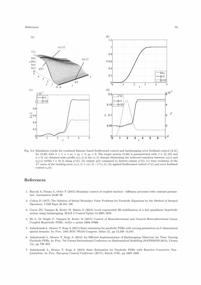
Control of PDEs - Startseite TU Ilmenau · Control of PDEs Lecture Notes for ... For further...

Prof. Dr.–Ing. habil. Thomas MeurerDr. Alexander Schaum

Control of PDEs

Lecture Notes for the Elgersburg School 2016

Date: February 2016

c© Lehrstuhl fur RegelungstechnikChristian–Albrechts–Universitat zu Kiel

Preface

These lecture notes are prepared for the Elgersburg School 2016 to be held in Elgersburg, Germany fromFebruary 28th to March 5th, 2016 and serve as a brief introduction to the analysis and control designfor systems governed by partial differential equations (PDEs). The topics address some extensions offlatness, backstepping and Lyapunov–based control to PDEs. It is in particular our desire to show boththeoretically and in certain selected experimental setups, that a combination of these approaches leadsto a systematic procedure for the design of stabilizing and robustifying tracking controllers for certainclasses of systems governed by (nonlinear) PDEs.

Kiel, February 2016 Prof. Dr.–Ing. habil. Thomas MeurerDr. Alexander Schaum

Chair of Automatic ControlFaculty of EngineeringChristian–Albrechts–University KielKaiserstrasse 2D–24143 Kiel, GermanyEmail: tm,[email protected]–kiel.de

iii

Contents

1 Introduction . . . . . . . . . . . . . . . . . . . . . . . . . . . . . . . . . . . . . . . . . . . . . . . . . . . . . . . . . . . . . . . . . . . . . . 1

1.1 Control of PDE systems . . . . . . . . . . . . . . . . . . . . . . . . . . . . . . . . . . . . . . . . . . . . . . . . . . . . . . . . . 1

1.2 Selected examples of distributed parameter systems . . . . . . . . . . . . . . . . . . . . . . . . . . . . . . . . . 2

1.2.1 Heat equation . . . . . . . . . . . . . . . . . . . . . . . . . . . . . . . . . . . . . . . . . . . . . . . . . . . . . . . . . . . . 3

1.2.2 Diffusion–convection–reaction systems . . . . . . . . . . . . . . . . . . . . . . . . . . . . . . . . . . . . . . 5

1.2.3 Flexible structures . . . . . . . . . . . . . . . . . . . . . . . . . . . . . . . . . . . . . . . . . . . . . . . . . . . . . . . . 7

1.3 Abstract formulation of linear PDEs . . . . . . . . . . . . . . . . . . . . . . . . . . . . . . . . . . . . . . . . . . . . . . 9

References . . . . . . . . . . . . . . . . . . . . . . . . . . . . . . . . . . . . . . . . . . . . . . . . . . . . . . . . . . . . . . . . . . . . . . . . . 11

2 Flatness–based trajectory planning and feedforward control design . . . . . . . . . . . . . . . 14

2.1 Finite–dimensional nonlinear control systems . . . . . . . . . . . . . . . . . . . . . . . . . . . . . . . . . . . . . . . 14

2.2 Distributed parameter control systems . . . . . . . . . . . . . . . . . . . . . . . . . . . . . . . . . . . . . . . . . . . . 16

2.2.1 Trajectory planning for PDE systems . . . . . . . . . . . . . . . . . . . . . . . . . . . . . . . . . . . . . . . 16

2.3 Operational calculus . . . . . . . . . . . . . . . . . . . . . . . . . . . . . . . . . . . . . . . . . . . . . . . . . . . . . . . . . . . . 17

2.3.1 Flatness–based trajectory planning for the linear heat equation . . . . . . . . . . . . . . . . . 17

2.3.2 Flatness–based trajectory planning for the linear wave equation . . . . . . . . . . . . . . . . 22

2.4 Riesz spectral operators . . . . . . . . . . . . . . . . . . . . . . . . . . . . . . . . . . . . . . . . . . . . . . . . . . . . . . . . . 24

2.4.1 Fundamental concepts . . . . . . . . . . . . . . . . . . . . . . . . . . . . . . . . . . . . . . . . . . . . . . . . . . . . 25

2.4.2 Flatness–based state and input parametrization . . . . . . . . . . . . . . . . . . . . . . . . . . . . . . 28

2.4.3 Application to the linear heat and wave equation with in–domain control . . . . . . . . 32

2.5 Extension to nonlinear problems . . . . . . . . . . . . . . . . . . . . . . . . . . . . . . . . . . . . . . . . . . . . . . . . . . 34

References . . . . . . . . . . . . . . . . . . . . . . . . . . . . . . . . . . . . . . . . . . . . . . . . . . . . . . . . . . . . . . . . . . . . . . . . . 35

3 Feedback stabilization and observer design using backstepping . . . . . . . . . . . . . . . . . . . . 39

3.1 Introduction to Lyapunov’s stability theory . . . . . . . . . . . . . . . . . . . . . . . . . . . . . . . . . . . . . . . . 39

3.2 Feedback control for a linear diffusion–reaction system using backstepping . . . . . . . . . . . . . 42

3.2.1 Stabilization problem . . . . . . . . . . . . . . . . . . . . . . . . . . . . . . . . . . . . . . . . . . . . . . . . . . . . . 42

iv

Contents v

3.2.2 Kernel computation . . . . . . . . . . . . . . . . . . . . . . . . . . . . . . . . . . . . . . . . . . . . . . . . . . . . . . 42

3.2.3 Solution of the kernel PDE . . . . . . . . . . . . . . . . . . . . . . . . . . . . . . . . . . . . . . . . . . . . . . . . 44

3.2.4 Inverse transformation . . . . . . . . . . . . . . . . . . . . . . . . . . . . . . . . . . . . . . . . . . . . . . . . . . . . 45

3.2.5 State–feedback controller and closed–loop stability . . . . . . . . . . . . . . . . . . . . . . . . . . . . 45

3.3 Tracking control for a semilinear diffusion–reaction system using flatness and backstepping 46

3.3.1 Flatness–based trajectory planning and feedforward control . . . . . . . . . . . . . . . . . . . . 47

3.3.2 Stabilization problem . . . . . . . . . . . . . . . . . . . . . . . . . . . . . . . . . . . . . . . . . . . . . . . . . . . . . 48

3.3.3 Kernel computation . . . . . . . . . . . . . . . . . . . . . . . . . . . . . . . . . . . . . . . . . . . . . . . . . . . . . . 49

3.3.4 Solution of the kernel PDE . . . . . . . . . . . . . . . . . . . . . . . . . . . . . . . . . . . . . . . . . . . . . . . . 50

3.3.5 Simulation results . . . . . . . . . . . . . . . . . . . . . . . . . . . . . . . . . . . . . . . . . . . . . . . . . . . . . . . . 51

3.4 Extensions of PDE backstepping . . . . . . . . . . . . . . . . . . . . . . . . . . . . . . . . . . . . . . . . . . . . . . . . . 52

References . . . . . . . . . . . . . . . . . . . . . . . . . . . . . . . . . . . . . . . . . . . . . . . . . . . . . . . . . . . . . . . . . . . . . . . . . 53

4 Lyapunov–based feedback stabilization and observer design . . . . . . . . . . . . . . . . . . . . . . . 55

4.1 Extensions to Lyapunov’s stability theory . . . . . . . . . . . . . . . . . . . . . . . . . . . . . . . . . . . . . . . . . 55

4.2 Vibration suppression for a flexible beam . . . . . . . . . . . . . . . . . . . . . . . . . . . . . . . . . . . . . . . . . . 57

4.2.1 Well-posedness of the model . . . . . . . . . . . . . . . . . . . . . . . . . . . . . . . . . . . . . . . . . . . . . . . 58

4.2.2 Lyapunov–based feedback control design . . . . . . . . . . . . . . . . . . . . . . . . . . . . . . . . . . . . 59

4.2.3 Lyapunov–based state–observer design . . . . . . . . . . . . . . . . . . . . . . . . . . . . . . . . . . . . . . 60

4.2.4 Stability of the composite system . . . . . . . . . . . . . . . . . . . . . . . . . . . . . . . . . . . . . . . . . . . 63

4.2.5 Experimental results . . . . . . . . . . . . . . . . . . . . . . . . . . . . . . . . . . . . . . . . . . . . . . . . . . . . . . 63

References . . . . . . . . . . . . . . . . . . . . . . . . . . . . . . . . . . . . . . . . . . . . . . . . . . . . . . . . . . . . . . . . . . . . . . . . . 65

Chapter 1

Introduction

Partial differential equations (PDEs) can be considered as the fundamental mathematical descriptionof many technical processes. In general, this distributed parameter description becomes an essentialingredient of the modeling and analysis process if the spatial or property–related distribution of theprocess variables can no longer be neglected. Following the exposition in [26] some characteristic examplesare summarized below:

• chemical or biochemical reactors [19] including three-way catalysts for exhaust gas after–treatmentin automotive applications, (reactive) distillation and adsorption processes [35], or activated sludgeprocesses for wastewater treatment [22];

• thermal systems [5] or the reheating and cooling of metal slabs during the steel processing to achievedesired metallurgical changes [40];

• electrochemical systems including fuel cells [36] and Li–ion or Li–polymer battery devices for energyproduction and storage [11, 15];

• smart materials, adaptive structures and resonant systems [24, 6, 27];

• flexible structures in aerospace and mechanical applications such as adaptive or flapping wing struc-tures [34], micro–mechanic bending cantilevers in atomic force microscopes [8], or deformable mirrorsin adaptive optics [31];

• fluid dynamical systems [1, 7], mixing processes and coupled fluid–structure interactions;

• wave propagation in optical fibers [33] and traffic congestion [41, 17];

• energy production in fusion reactors [37, 3].

The dynamic operation of these distributed parameter systems (DPSs) essentially relies on the incor-poration of suitable control strategies to influence the system dynamics and to enlarge the operatingrange.

1.1 Control of PDE systems

The so–called two–degrees–of–freedom (2DOF) control concept , that forms the basis for these lecturenotes, is schematically shown in Figure 1.1. Given the distributed parameter system Σ∞ with outputy(t), the control structure comprises trajectory planning Σ∗ and feedforward control Σff to impose thedesired output trajectory y∗(t) by means of u∗(t) and feedback control Σe

fbto provide the state–feedbackue(t) in terms of the estimated error state xe(t) obtained from an error system observer Σe

ob processingthe tracking error ye(t) = y(t) − y∗(t). In the nominal case of an exact plant model Σ∞, no exogenousdisturbances and perfectly known initial conditions the feedforward control in combination with trajectory

1

2 1 Introduction

Σ∗ Σff

Σefb

Σeob

Σ∞y∗ u∗ u y

ye −xe

ue

Fig. 1.1: Block diagram of the 2DOF control concept for the DPS Σ∞ with trajectory planning Σ∗, feedforward controlΣff , error feedback control Σefb, error system observer Σeob for tracking control y → y∗.

planning ensures that the output y(t) exactly tracks a prescribed desired trajectory y∗(t). To accountfor model uncertainties, disturbances and instability a feedback controller is designed to stabilize thetracking error dynamics, i.e. the evolution of the deviation between the actual state and its desired value.The latter is herein known from the flatness–based state and input parametrization. Moreover, it is ingeneral necessary to integrate a distributed parameter state–observer to estimate the unmeasured stateevolution from the available measurements.

The model–based control and observer design for distributed parameter systems1 can be in generalclassified into early and late lumping techniques. While in the early lumping approach, the governingPDEs are reduced to a finite–dimensional description by making use of suitable approximation and modelreduction techniques prior to the feedback control design the late lumping approach directly exploitsthe system formulation in terms of PDEs. In the following, only late lumping design techniques areaddressed and if needed combined with suitable approximation methods for implementation. Followingthe schematics in Figure 1.1 the lecture notes cover

• flatness–based trajectory planning and feedforward control for PDEs,

• backstepping techniques for state–feedback control and observer design and

• Lyapunov– or passivity–based output feedback control.

Introductions and a brief literature survey are provided in the individual chapters. Since mathematicalmodels are the common starting point for any development, in the following a summary of selectedPDE control problems is provided, that serve as basis for the application of flatness–, backstepping– andpassivity–based control as well as their combination.

1.2 Selected examples of distributed parameter systems

Subsequently, distributed parameter models are summarized covering selected control examples. Wheredirectly possible Matlab code is provided for the numerical simulation and the later evaluation of thecontrol concepts.

1 This section does not aim to provide a comprehensive review of existing analysis and control design techniques for PDEsystems. For this, the reader is referred, e.g., to [12, 23, 39, 26].

1.2 Selected examples of distributed parameter systems 3

1.2.1 Heat equation

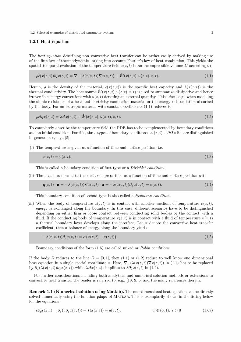
The heat equation describing non–convective heat transfer can be rather easily derived by making useof the first law of thermodynamics taking into account Fourier’s law of heat conduction. This yields thespatial–temporal evolution of the temperature field x(z, t) in an incompressible volume Ω according to

ρc(x(z, t))∂tx(z, t) = ∇ ·(λ(x(z, t))∇x(z, t)

)+ W (x(z, t), u(z, t), z, t). (1.1)

Herein, ρ is the density of the material, c(x(z, t)) is the specific heat capacity and λ(x(z, t)) is thethermal conductivity. The heat source W (x(z, t), u(z, t), z, t) is used to summarize dissipative and henceirreversible energy conversions with u(z, t) denoting an external quantity. This arises, e.g., when modelingthe ohmic resistance of a heat and electricity conduction material or the energy rich radiation absorbedby the body. For an isotropic material with constant coefficients (1.1) reduces to

ρc∂tx(z, t) = λ∆x(z, t) + W (x(z, t), u(z, t), z, t). (1.2)

To completely describe the temperature field the PDE has to be complemented by boundary conditionsand an initial condition. For this, three types of boundary conditions on (z, t) ∈ ∂Ω×R+ are distinguishedin general, see, e.g., [5]:

(i) The temperature is given as a function of time and surface position, i.e.

x(z, t) = v(z, t). (1.3)

This is called a boundary condition of first type or a Dirichlet condition.

(ii) The heat flux normal to the surface is prescribed as a function of time and surface position with

q(z, t) · n = −λ(x(z, t))∇x(z, t) · n = −λ(x(z, t))∂nx(z, t) = v(z, t). (1.4)

This boundary condition of second type is also called a Neumann condition.

(iii) When the body of temperature x(z, t) is in contact with another medium of temperature v(z, t),energy is exchanged along the boundary. In this case, different scenarios have to be distinguisheddepending on either firm or loose contact between conducting solid bodies or the contact with afluid. If the conducting body of temperature x(z, t) is in contact with a fluid of temperature v(z, t)a thermal boundary layer develops along the interface. Let α denote the convective heat transfercoefficient, then a balance of energy along the boundary yields

−λ(x(z, t))∂nx(z, t) = α(x(z, t)− v(z, t)

). (1.5)

Boundary conditions of the form (1.5) are called mixed or Robin conditions.

If the body Ω reduces to the line Ω = [0, 1], then (1.1) or (1.2) reduce to well–know one–dimensionalheat equation in a single spatial coordinate z . Here, ∇ · (λ(x(z, t))∇x(z, t)) in (1.1) has to be replacedby ∂z (λ(x(z, t))∂zx(z, t)) while λ∆x(z, t) simplifies to λ∂2

zx(z, t) in (1.2).

For further considerations including both analytical and numerical solution methods or extensions toconvective heat transfer, the reader is referred to, e.g., [10, 9, 5] and the many references therein.

Remark 1.1 (Numerical solution using Matlab). The one–dimensional heat equation can be directlysolved numerically using the function pdepe of Matlab. This is exemplarily shown in the listing belowfor the equations

c∂tx(z, t) = ∂z (a∂zx(z, t)) + f(x(z, t)) + u(z, t), z ∈ (0, 1), t > 0 (1.6a)

4 1 Introduction

∂zx(0, t) = 0, x(1, t) = v(t), t ≥ 0 (1.6b)

x(z, 0) = 0, z ∈ [0, 1] (1.6c)

with

f(x(z, t)) = 5(x(z, t))2 − x(z, t)

u(z, t) = 0

v(t) = (t− 0.5)σ(t− 0.5)− 2(t− 1)σ(t− 1) + (t− 1.5)σ(t− 1.5)

(1.6d)

Herein, σ(t) denotes the Heaviside function.

function out=heateqn()

%

%Numerical solution of the linear heat equation using MATLAB.

%(c) Thomas Meurer, CAU Kiel

%------------------------

% MAIN

%Preparations

m=0;

zmax=1.0;

tmax=2.0;

z=linspace(0,zmax,101);

t=linspace(0,tmax,201);

%System parameters and functions

a=1.0;

f=inline(’-x+5*x^2’,’x’);

u=inline(’0’,’z’,’t’);

v=inline(’(t-0.5).*stepfun(t,0.5)-2*(t-1).*stepfun(t,1)...

+(t-1.5).*stepfun(t,1.5)’,’t’);

%Solver call

sol=pdepe(m,@heat_pde,@heat_ic,@heat_bc,z,t,[],a,f,u,v);

x=sol(:,:,1);

%Output

out.z = z; out.t = t; out.x = x;

%Surface plot

figure; mesh(z,t,x); xlabel(’z’); ylabel(’t’);

%------------------------

% SUBFUNCTIONS

function [c,g,s]=heat_pde(z,t,x,DxDz,a,f,u,v)

%Partial differential equation

c = 1.0;

g = a*DxDz;

s = f(x) + u(z,t);

function u0=heat_ic(z,a,f,u,v);

%Initial condition

x0 = 0.0;


function [pl,ql,pr,qr]=heat_bc(zl,xl,zr,xr,t,a,f,u,v)

%Boundary conditions

pl=0.0;

ql=1.0;

pr=xr-v(t);

qr=0.0;

The solution is thereby determined by a so–called method–of–lines approach, where the PDE is semi–discretized in the spatial coordinate.

1.2.2 Diffusion–convection–reaction systems

Fixed–bed or tubular reactors are among the most common types of chemical conversion devices inchemical engineering. Herein, a rather complex interplay of diffusive, convective and reactive effects arises,that has to be captured in mathematical process models. Figure 1.2 shows a schematic (differential) controlvolume of a fixed–bed reactor, that is packed by some catalyst. Typically reactants are led through thereactor in gaseous state with chemical reactions being initiated at the surface of the catalyst.

z z + dzz

Catalyst

Voidage

Cooling jacket

T,wj

p, ρ, v

Fig. 1.2: Differential reactor element with inflow temperature T , mass fraction wj , pressure p, density ρ, fluid velocity v.

Taking into account global mass balance, componentwise mass balances, energy or enthalpy balance,impulse balances, and thermodynamics equations of state the reactor modeling results in a descriptionin terms of coupled hyperbolic (and/or parabolic) PDEs. Depending on the desired level of detail andresolution highly complex models are obtained (see, e.g., [19]), that are hardly accessible for controldesign. Hence, different simplifications are typically introduced related to fluid flow in the reactor (e.g.,plug flow assumption), dimension (e.g., one–dimensional compared to three–dimensional spatial domain)or the parametrization of the reaction rates (e.g., linear or nonlinear dependency on mass fractions ormolar concentrations, respectively).

As an example, a distributed parameter description of the form

∂tx(z, t) = ∂z [D(z,x(z, t))∂zx(z, t))] + f(z,x(z, t), ∂zx(z, t),u(t)), (z, t) ∈ (0, L), t > 0 (1.7a)

g0(x(0, t), ∂zx(0, t),v0(t)) = 0,

gL(x(L, t), ∂zx(L, t),vL(t)) = 0,t ≥ 0 (1.7b)

6 1 Introduction

x(z, 0) = x(0, z), z ∈ [0, L] (1.7c)

does seem appropriate to reflect the dominating dynamics. Herein, D(z,x(z, t)) is the diffusion matrix,f(z,x(z, t), ∂zx(z, t),u(t)) represents reactive and convective effects, arising nonlinearities, and inhomo-geneous terms u(t), g0(·) and gL(·) refer to in general non–autonomous boundary conditions, and x(0, z)is the initial reactor state. The state vector x(z, t) may comprise mass fractions (or molar concentrations)and temperatures. Considering the reactor in a neighborhood of an operating profile, i.e., a steady statesolution of (1.7), then linearization of (1.7) yields a (local) system formulation in the form of a lineardiffusion–convection–reaction system

∂tx(z, t) = D(z)∂2zx(z, t) + C(z)∂zx(z, t) +R(z)x(z, t) +B(z)u(t), (z, t) ∈ (0, L), t > 0 (1.8a)

G0x(0, t) + F0∂zx(0, t)) = H0v0(t),

GLx(L, t) + FL∂zx(L, t)) = HLvL(t),t ≥ 0 (1.8b)

x(z, 0) = x0(z), z ∈ [0, L]. (1.8c)

Herein, D(z), C(z) and R(z) denote diffusion, convection and reaction matrices, respectively. For furtherdetails on the mathematical modeling of reaction engineering applications using distributed parametersystems the reader is referred, e.g., to [4, 9, 19].

Remark 1.2 (Numerical solution using Matlab). For the one–dimensional setting with z ∈ [0, L],L ∈ R+ the function pdepe of Matlab can be used for the numerical solution of both the nonlinear PDEsystem (1.7) and the linear PDE system (1.8). For this, the assumption has to be made, that

g0(x(0, t), ∂zx(0, t),v0(t)) = D(0,x(0, t))∂zx(0, t) + p0(x(0, t),v0(t))

gL(x(L, t), ∂zx(L, t),vL(t)) = D(L,x(L, t))∂zx(L, t) + pL(x(L, t),vL(t))(1.9)

A similar relationship has to hold for (1.8b). The following listing provides an implementation of (1.7),(1.9). Here, the arising matrix– and vector–valued functions are assumed to be available on the Matlabpath with the corresponding number of input arguments.

function out=dcrs()

%

%Numerical solution of a vector-valued diffusion-convection-reaction

%system using MATLAB.

%(c) Thomas Meurer, CAU Kiel

%------------------------

% MAIN

%Preparations

m=0;

zmax=1.0;

tmax=2.0;

z=linspace(0,zmax,101);

t=linspace(0,tmax,201);

%System parameters and functions

h.D = @fun_D;

h.f = @fun_f;

h.p0 = @fun_p0;

h.pL = @fun_pL;

h.x0 = @fun_x0;

%% alternatively define inline or as subfunctions


%Solver call

sol=pdepe(m,@dcrs_pde,@dcrs_ic,@dcrs_bc,z,t,[],h);

%Output

out.z = z; out.t = t; out.x = sol;

%------------------------

% SUBFUNCTIONS

function [c,g,s]=dcrs_pde(z,t,x,DxDz,h)

%Partial differential equation

c = ones(size(x,1),1);

g = h.D(z,x)*DxDz;

s = h.f(z,x,DxDz,t);

function x0=dcrs_ic(z,h);

%Initial condition

x0 = h.x0(z);

function [pl,ql,pr,qr]=dcrs_bc(zl,xl,zr,xr,t,h)

%Boundary conditions

E = ones(size(xl,1),1);

pl = h.p0(xl,t);

ql = E;

pr = h.pL(xr,t);

qr = E;

As alternative numerical solution techniques consider, e.g., the weighted residual or Galerkin approach[13] or finite difference techniques [38].

1.2.3 Flexible structures

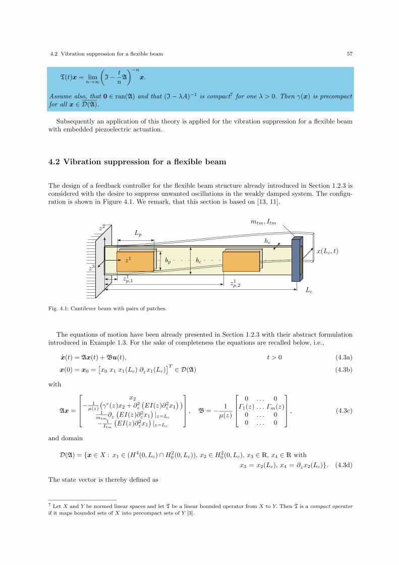
Flexible structures with embedded actuators and sensors arise in a broad variety in different applicationsincluding large scale manipulators [18], lightweight robotics and adaptive structures [24, 6, 14, 28, 27], orfluid–structure interaction [20, 21]. For a detailed introduction to the mathematical modeling of flexiblestructures using, e.g., the extended Hamilton’s principle, the reader is referred to [29, 25, 16, 30].

In the following, only the wave equation and the Euler–Bernoulli beam equation are presented asexamples for PDEs modeling flexible structures. Considering, e.g., the transversal motion of a string, thetorsional motion of a rod or the longitudinal deflection of a beam mathematical modeling leads to thewave equation which, in the linear case, is governed by

∂2t x(z, t) = c2∂2

zx(z, t)− α∂tx(z, t)− β∂zx(z, t) + γx(z, t) + b(z)u(t), (z, t) ∈ (0, L), t > 0 (1.10a)

∂zx(0, t) + p0x(0, t) = v0(t),

∂zx(L, t) + pLx(L, t) = vL0(t),t ≥ 0 (1.10b)

x(z, 0) = x0(z), ∂tx(z, 0) = x1(z), z ∈ [0, L]. (1.10c)

Here, c denotes the speed of wave propagation (for a discussion on dispersion, phase and group velocitythe reader is referred to, e.g., [41]), α denotes a temporal damping coefficient, β is a spatial dampingcoefficient, and γ, p0, pL are some parameters. The wave equation is a prototypical example of a hyperbolicPDE which, contrary to the heat equation (1.1), exhibits a finite speed of propagation. Due to thisproperty hyperbolic PDEs cannot be directly solved using standard numerical tools such as the pdepe

function of Matlab but require special emphasis when discretizing the PDE and boundary conditions.

8 1 Introduction

To motivate the Euler–Bernoulli beam equation consider the cantilevered beam structure with tipmass depicted in Figure 1.3. The beam is actuated by pairs of piezoelectric patch actuators, where thepatches on the front side (fs) and the patches on the back side (bs) are bonded symmetrically onto thebeam structure. The mounted piezoelectric actuators allow to locally induce bending strains within the

z1

z3

z2

Lc

bc

hc

z1p,1 z1

p,2

mtm, Itm

bp

Lp

x(Lc, t)

Fig. 1.3: Cantilever beam with pairs of patches.

patch covered intervals [z1p,k, z

1p,k + Lp] of the beam domain defined by

Λεk(z1) =(%ε(z1 − z1

p,k)− %ε(z1 − z1p,k − Lp)

), (1.11)

where %ε(z1) represents a (possibly smooth) transition function from %ε(z1) = 0 for z1 < −ε/2 to%ε(z1) = 1 for z1 > ε/2. Here, Lc and Lp denote the length of the beam and the patches, respectively.Considering the individual patch contributions to stiffness, damping, and inertia, this configuration resultsin a beam model with spatially varying parameters such that the governing equations of motion for thebeam deflection x(z, t) are given by

µ(z1)∂2t x(z1, t) + γe(z1)∂tx(z1, t) + ∂2

z1

(EI(z1)∂2

z1x(z1, t))

= −m∑k=1

Γk(z1)uk(t) (1.12a)

with the boundary conditions

x(z1, t) = 0, ∂z1x(z1, t) = 0, z1 = 0 (1.12b)

EI(z1)∂2z1x(z1, t) + Itm∂

2t ∂z1x(z1, t) = 0,

∂z1(EI(z1)∂2

z1x(z1, t))−mtm∂

2t x(z1, t) = 0.

z1 = Lc (1.12c)

and the initial conditions

x(z1, 0) = x0(z1), ∂tx(z1, 0) = x1(z1). (1.12d)

The coefficients µ(z1), γe(z1), EI(z1) denote mass per unit length, viscous damping and stiffness, respec-tively, and are given by

µ(z1) = µc + 2

m∑k=1

Λεk(z1)µp (1.13)

γe(z1) = γec + 2

m∑k=1

Λεk(z1)γep (1.14)

EI(z1) = EIc + 2

m∑k=1

Λεk(z1)EIp. (1.15)

The in–domain actuation is given in terms of

1.3 Abstract formulation of linear PDEs 9

Γk(z1) = Γp,k∂2z1Λ

εk(z1), (1.16)

where Γp,k summarizes patch actuator specific parameters. Additionally, mtm denotes the mass and Itmthe inertia of the tip mass. Here, the indices c, p and tm indicate the contributions of the carrier layer,the patches and the tip mass, respectively. The equations of motion (1.12) can be directly determined bymeans of the extended Hamilton’s principle using calculus of variations [32]. The distributed parametersystem (1.12) is a so–called biharmonic PDE due to the arising forth order differentiation in z1. For thenumerical solution of (1.12) either weighted residual methods, Galerkin methods, finite element methods,or the Rayleigh–Ritz ansatz can be applied, see, e.g., [25].

1.3 Abstract formulation of linear PDEs

For the mathematical analysis and control design it is often advantageous to rewrite the governing PDEsas a so–called abstract Cauchy problem [12, 39]. Given a linear distributed parameter systems the abstractformulation resembles the well–known state space formulation for linear finite–dimensional systems andtakes the form

x(t) = Ax(t) + Bu(t), t > 0 (1.17a)

x(0) = x0 ∈ D(A). (1.17b)

Here, a state vector x(t) ∈ X from some Hilbert space X is introduced with A referring to a lineardifferential operator, that maps elements of its domain D(A) to X. The operator B denotes the inputoperator which maps the input u(t) ∈ U to X.

In the following it is assumed, that the reader is familiar with basics on linear function spaces. For thesake of completeness some examples of Hilbert spaces, i.e., normed linear spaces equipped with an innerproduct 〈·, ·〉X , are provided, that are useful for the subsequent analysis:

• Space of Lebesgue measurable functions Lp(a, b): Let p ≥ 1 be a fixed integer and let a, b ∈ R. We

denote by Lp(a, b) the set of measurable functions x(t) with∫ ba|x(t)|pdt < ∞ equipped with the

norm2

‖x‖Lp =

(∫ b

a

|x(t)|pdt) 1p

. (1.18)

For p = 2 an inner product on L2(a, b) can be introduced by

〈x(t), y(t)〉L2 =

∫ b

a

x(t)y(t)dt, 〈x(t), x(t)〉L2 = ‖x‖2L2 (1.19)

given x(t), y(t) ∈ L2. If p =∞, then the norm is defined as

‖x‖L∞ = ess supt∈[a,b]

|x(t)| (1.20)

provided, that ess supt∈[a,b] |x(t)| <∞.

• Sobolev spaces Hp(a, b): Let p ≥ 1 be a fixed integer and let a, b ∈ R. The subspace of L2(a, b) definedby

Hp(a, b) =x(t) ∈ L2(a, b) : ∂jt x(t) ∈ L2(a, b), j = 0, 1, . . . , p

(1.21)

2 One actually needs to consider equivalence classes since ‖x‖Lp = 0 implies x(t) = 0 only almost everywhere. For detailsconsult, e.g., [12].

10 1 Introduction

equipped with the inner product

〈x(t), y(t)〉Hp =

p∑j=0

⟨∂jt x(t), ∂jt y(t)

⟩L2 (1.22)

is a Hilbert space. It can be shown, that Hp(a, b) is the completion of Cp(a, b) or C∞(a, b) functionwith respect to the norm (1.22). Note also the embedding Hp+1(a, b) ⊂ Hp(a, b). For details onSobolev spaces and their properties the reader is referred to [2].

With these preparations the examples introduced before, i.e., the heat equation, the wave equation andthe Euler–Bernoulli beam, can be transferred into the abstract formulation (1.17).

Example 1.1 (Heat equation). Consider the linear heat equation, i.e.,

c∂tx(z, t) = a∂2zx(z, t)) + u(z, t), z ∈ (0, 1), t > 0 (1.23a)

∂zx(0, t = 0, x(1, t) = 0, t ≥ 0 (1.23b)

x(z, 0) = 0, z ∈ [0, 1]. (1.23c)

The consideration of inhomogeneous boundary conditions requires special emphasis in the context of theabstract setting so that only homogeneous boundary conditions are assumed for the sake of simplicity.Taking x(t) = x(·, t), u(t) = u(·, t), x0 = x0(·), and introducing X = L2(0, 1) as solution space we obtain

x(t) = Ax(t) + bu(t), t > 0 (1.24a)

x(0) = x0 (1.24b)

with

Ax =a

c∂2zx, b =

1

c(1.24c)

and domain

D(A) =x ∈ X : ∂2

zx ∈ L2(0, 1) with ∂zx(0) = 0, x(1) = 0. (1.24d)

Example 1.2 (Wave equation). Consider (1.10) for homogeneous boundary conditions, i.e.,

∂2t x(z, t) = c2∂2

zx(z, t)− α∂tx(z, t)− β∂zx(z, t) + γx(z, t) + b(z)u(t), (z, t) ∈ (0, L), t > 0 (1.25a)

x(0, t) = 0,

∂zx(L, t) = 0,t ≥ 0 (1.25b)

x(z, 0) = x0(z), ∂tx(z, 0) = x1(z), z ∈ [0, L]. (1.25c)

As is common for finite–dimensional second order systems a state vector has to be introduced to obtain aformulation as coupled system of first order ODEs or PDEs, respectively. Hence, let

x(t) =

[x1(t)x2(t)

]=

[x(·, t)∂tx(·, t)

](1.26)

and consider X = H10 (0, L)× L2(0, L) with H1

0 (0, L) = x ∈ H1(0, L) : x(0) = 0 as solution space withinner product and induced norm

〈x,y〉X = c2〈x1, y1〉H1 + 〈x2, y2〉L2 , ‖x‖2X = 〈x,x〉X (1.27)

for x, y ∈ X. The motivation to introduce this particular Hilbert space is given by consideration of theenergy stored in the (undamped) system which directly corresponds to 1

2 〈x,x〉X as sum of potential andkinetic energy. With this, we obtain

x(t) = Ax(t) + bu(t), t > 0 (1.28a)

References 11

x(0) = x0 =[x0 x1

]T ∈ D(A) (1.28b)

with

Ax =

[x2

c2∂2zx1 − αx2 − β∂zx1 + γx1

], b =

[0b(z)

](1.28c)

and domain

D(A) = x ∈ X : x1 ∈ (H2(0, L) ∩H10 (0, L)), x2 ∈ H1(0, L) with ∂zx1(L) = 0. (1.28d)

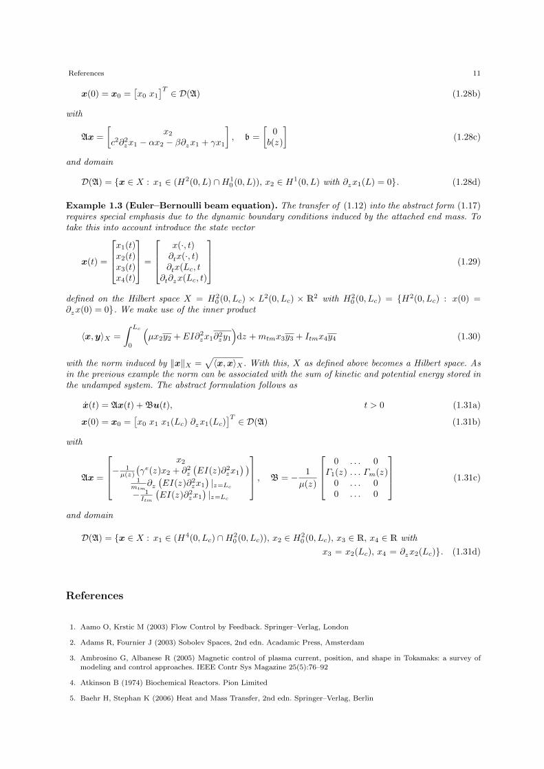
Example 1.3 (Euler–Bernoulli beam equation). The transfer of (1.12) into the abstract form (1.17)requires special emphasis due to the dynamic boundary conditions induced by the attached end mass. Totake this into account introduce the state vector

x(t) =

x1(t)x2(t)x3(t)x4(t)

=

x(·, t)∂tx(·, t)∂tx(Lc, t

∂t∂zx(Lc, t)

(1.29)

defined on the Hilbert space X = H20 (0, Lc) × L2(0, Lc) × R2 with H2

0 (0, Lc) = H2(0, Lc) : x(0) =∂zx(0) = 0. We make use of the inner product

〈x,y〉X =

∫ Lc

0

(µx2y2 + EI∂2

zx1∂2zy1

)dz +mtmx3y3 + Itmx4y4 (1.30)

with the norm induced by ‖x‖X =√〈x,x〉X . With this, X as defined above becomes a Hilbert space. As

in the previous example the norm can be associated with the sum of kinetic and potential energy stored inthe undamped system. The abstract formulation follows as

x(t) = Ax(t) + Bu(t), t > 0 (1.31a)

x(0) = x0 =[x0 x1 x1(Lc) ∂zx1(Lc)

]T ∈ D(A) (1.31b)

with

Ax =

x2

− 1µ(z)

(γe(z)x2 + ∂2

z

(EI(z)∂2

zx1

) )1

mtm∂z(EI(z)∂2

zx1

)|z=Lc

− 1Itm

(EI(z)∂2

zx1

)|z=Lc

, B = − 1

µ(z)

0 . . . 0

Γ1(z) . . . Γm(z)0 . . . 00 . . . 0

(1.31c)

and domain

D(A) = x ∈ X : x1 ∈ (H4(0, Lc) ∩H20 (0, Lc)), x2 ∈ H2

0 (0, Lc), x3 ∈ R, x4 ∈ R with

x3 = x2(Lc), x4 = ∂zx2(Lc). (1.31d)

References

1. Aamo O, Krstic M (2003) Flow Control by Feedback. Springer–Verlag, London

2. Adams R, Fournier J (2003) Sobolev Spaces, 2nd edn. Acadamic Press, Amsterdam

3. Ambrosino G, Albanese R (2005) Magnetic control of plasma current, position, and shape in Tokamaks: a survey ofmodeling and control approaches. IEEE Contr Sys Magazine 25(5):76–92

4. Atkinson B (1974) Biochemical Reactors. Pion Limited

5. Baehr H, Stephan K (2006) Heat and Mass Transfer, 2nd edn. Springer–Verlag, Berlin

12 1 Introduction

6. Banks H, Smith R, Wang Y (1996) Smart Material Structures: Modeling, Estimation and Control. John Wiley & Sons,

Chichester

7. Bewley T (2000) Flow control: New Challenges for a new Renaissance. Prog Aerosp Sci 37:21–58

8. Bining G, Quate C, Gerber C (1986) Atomic force microscope. Phys Rev Letter 56(9):930–933

9. Bird R, Stewart W, Lightfoot E (2002) Transport Phenomena, 2nd edn. John Wiley & Sons, Inc., New York

10. Carslaw H, Jaeger J (1959) Conduction of Heat in Solids, 2nd edn. Oxford University Press, Oxford

11. Chen Y, Evans J (1996) Thermal analysis of lithium-ion batteries. J Electrochem Soc 143(9):2708–2712

12. Curtain R, Zwart H (1995) An Introduction to Infinite–Dimensional Linear Systems Theory. Texts in Applied Mathe-

matics 21, Springer–Verlag, New York

13. Fletcher C (1984) Computational Galerkin Methods. Springer–Verlag, New York

14. Gawronski W (1998) Dynamics and Control of Structures. Springer–Verlag, New York

15. Gu W, Wang C (2000) Thermal–Electrochemical Modeling of Battery Systems. J Electrochem Soc 147(8):2910–2922

16. Haupt P (2002) Continuum Mechanics and Theory of Materials, 2nd edn. Springer–Verlag, Berlin Heidelberg

17. Helbing D (2001) Traffic and related self–driven many-particle systems. Rev Mod Phys 73(4):1067–1141

18. Henikl J, Kemmetmuller W, Meurer T, Kugi A (2016) Infinite–Dimensional Decentralized Damping Control of Large–

Scale Manipulators with Hydraulic Actuation. Automatica 63(1):101–115

19. Jakobsen H (2008) Chemical Reactor Modeling – Multiphase Reactive Flows. Springer, Berlin Heidelberg

20. King R (ed) (2007) Active Flow Control, Notes on Numerical Fluid Mechanics and Multidisciplinary Design, vol 95.

Springer–Verlag, Berlin, Heidelberg

21. King R (ed) (2010) Active Flow Control II, Notes on Numerical Fluid Mechanics and Multidisciplinary Design, vol 108.

Springer–Verlag, Berlin, Heidelberg

22. Lee T, Wang F, Newell R (2006) Advances in distributed parameter approach to the dynamics and control of activatedsludge processes for wastewater treatment. Water Research 40(5):853–869

23. Luo Z, Guo B, Morgul O (1999) Stability and Stabilization of Infinite Dimensional Systems with Applications. Springer–

Verlag, London

24. Meirovitch L (1990) Dynamics and Control of Structures. Wiley, New York

25. Meirovitch L (1997) Principles and Techniques of Vibrations. Prentice Hall, New Jersey

26. Meurer T (2013) Control of Higher–Dimensional PDEs: Flatness and Backstepping Designs. Communications and

Control Engineering Series, Springer–Verlag

27. Preumont A (2002) Vibration Control of Active Structures, 2nd edn. Kluwer Academic, Dordrecht

28. Rahn C (2001) Mechatronic Control of Distributed Noise and Vibration – A Lyapunov Approach. Springer–Verlag,

Berlin

29. Reddy J (1984) Energy and Variational Methods in Applied Mechanics. Wiley–Interscience, New York

30. Reddy J (2007) Theory and Analysis of Elastic Plates and Shells, 2nd edn. Taylor & Francis

31. Roddier F (ed) (1999) Adaptive Optics in Astronomy. Cambridge University Press, Cambridge

32. Schrock J (2012) Mathematical Modeling and Tracking Control of Piezo–actuated Flexible Structures. Shaker–Verlag

33. Shaw J (2004) Mathematical Principles of Optical Fiber Communications. SIAM, Philadelphia

34. Stanewsky E (2001) Adaptive wing and flow control technology. Prog Aerosp Sci 37:583–667

35. Sundmacher K, Kienle A (eds) (2002) Reactive Distillation – Status and Future Directions. Wiley–VCH, Weinheim

36. Sundmacher K, Kienle A, Pesch H, Berndt J, Huppmann G (eds) (2007) Molten Carbonate Fuel Cells: Modeling,Analysis, Simulation, and Control. Wiley–VCH Verlag GmbH, Weinheim

37. Taylor T (1997) Physics of advanced tokamaks. Plasma Physics and Controlled Fusion 39(12B):B47

38. Thomas J (1998) Numerical Partial Differential Equations: Finite Difference Methods, Texts in Applied Mathematics,

vol 22. Springer–Verlag, New York

References 13

39. Tucsnak M, Weiss G (2009) Observation and Control for Operator Semigroups. Birkhauser, Basel

40. Unger A, Troltzsch F (2001) Fast Solution of Optimal Control Problems in the Selective Cooling of Steel. Z AngewMath Mech 81(7):447–456

41. Whitham G (1999) Linear and Nonlinear Waves. John Wiley & Sons, New York

Chapter 2

Flatness–based trajectory planning and feedforwardcontrol design

The notion of (differential) flatness, as introduced by M. Fliess and co–workers [4, 6], has turned out toprovide a useful approach for solving trajectory tracking problems [33, 20, 28, 21, 36, 44]. Originally, theconcept was formulated for finite–dimensional nonlinear systems but many aspects have been successfullygeneralized to certain classes of infinite-dimensional systems. In this chapter, we provide an introduction toflatness–based techniques by first summarizing some results obtained for the finite–dimensional case. Thisis followed by illustrating different extensions of this approach to infinite–dimensional systems governedby distributed parameter systems.

2.1 Finite–dimensional nonlinear control systems

Roughly speaking, flatness means, that there exists a so-called flat or basic output such that all systemvariables (states, inputs and outputs) can be parametrized in terms of this flat output and its timederivatives1. For the sake of simplicity let us consider a nonlinear system of the form

x = f(x,u) (2.1)

with the state x(t) ∈ X ⊂ Rn and the input u(t) ∈ U ⊂ Rm. The system (2.1) is called flat if there existsa so-called flat or basic output ξ(t) such that [4, 32, 36]

(i) the components of ξ(t) are functions of x(t) and u(t) and their time derivatives2

ξ = φ(x,u, u, . . . ,u(γ)

), (2.2)

(ii) the components of ξ(t) are not related by any differential or algebraic equation of the form3

ϕ(ξ, ξ, . . . , ξ(δ)

)= 0 , (2.3)

(iii) and all system variables can be parametrized by the flat output and its time derivatives

x = ψ1

(ξ, ξ, . . . , ξ(β)

)u = ψ2

(ξ, ξ, . . . , ξ(β+1)

).

(2.4)

1 As will be shown in subsequent sections for infinite–dimensional systems governed by PDEs an infinite number of time

derivatives of the flat output may be required.2 Here and subsequently we will denote the γth time derivative of a function f (t) in the form f (γ) = ∂γt f(t) .3 This condition is equivalent to dimu = dim ξ.

14

2.1 Finite–dimensional nonlinear control systems 15

Example 2.1 ((Linear time invariant system). A linear time-invariant system is flat if and only ifit is controllable. A controllable linear system can be always transformed into the controllability normalform which for SISO systems is given by

x1

x2

...xn−1

xn

︸︷︷︸

x

=

0 1 0 . . . 00 0 1 . . . 0...

.... . .

. . ....

0 0 . . . 0 1−a0 −a1 . . . −an−2 −an−1

︸︷︷︸

A

x1

x2

...xn−1

xn

︸︷︷︸

x

+

00...01

︸︷︷︸b

u (2.5)

with the coefficients aj, j = 1, . . . , n, of the characteristic polynomial of the matrix A ∈ Rn×n. Obviously,ξ(t) = x1(t) serves as a flat output and the state and input parametrization according to (2.4) reads

xj = ξ(j−1), j = 1, 2, . . . , n (2.6)

u =

n∑j=0

ajξ(j) (2.7)

with an = 1 and ξ(0)(t) = ξ(t).

In view of the analysis of distributed parameter systems some essential properties of flat finite–dimensionalnonlinear control systems are summarized below:

• Steady state analysis: The state and input parametrizations (2.4) can be similarly used to analyze

the steady state behavior, i.e. let ξ(t) = ξs, ξ(j) = 0, j ≥ 1 and consider 0 = f(xs,us), then

xs = ψ1(ξs,0, . . . ,0) = ψ1(ξs)

us = ψ2(ξs,0, . . . ,0) = ψ2(ξs).

This property will play a substantial role for distributed parameter systems.

• Uniqueness of flat outputs: Flat systems may have more than a single flat output fulfilling the condi-tions (2.2)–(2.4). In this case (differential) relations exist, that allow to transfer one flat output intothe other.

• Uncontrolled systems: Free (uncontrolled) systems x(t) = f(x(t)) are not flat. Assume for the mo-

ment, that there exists a flat output ξ(t) with x(t) = ψ1

(ξ(t), ξ(t), . . . , ξ(β)(t)

). Then substitution

of this expression into the differential equation yields a differential equation of the form (2.3) whichcontradicts the assumption.

• Linear time invariant systems: For linear time invariant systems flatness and controllability are equiv-alent (see Example 2.1).

• Existence of flat outputs: For the flatness of nonlinear SISO systems necessary and sufficient conditionsexist which are well-known from the theory of exact input–state linearization. In fact for SISO systemsexact input–state linearizability and flatness are equivalent. For MIMO systems also necessary andsufficient conditions are available for a nonlinear system to be exactly input–state linearizable, see,e.g., [12, 29]. In the last years much effort has been made in finding conditions for a MIMO systemto be flat, see, e.g., [17, 39, 42]. However, if a MIMO system is exact input–state linearizable, then itis also flat.

• Flatness–based feedforward control: Let ξ∗(t) ∈ Cn(R) denote a desired trajectory for the flat output.Then substitution of ξ∗(t) into (2.4) directly yields the feedforward control u∗(t), that is required torealize x(t)→ x∗(t) in open–loop without integration of any differential equation, i.e.

16 2 Flatness–based trajectory planning and feedforward control design

x∗ = ψ1

(ξ∗, ξ∗, . . . , ξ∗ (β)

)u∗ = ψ2

(ξ∗, ξ∗, . . . , ξ∗ (β+1)

).

(2.8)

The determined trajectories x(t) and u(t) can be in advance utilized to analyze the fulfillment of stateand input constraints. In addition, x∗(t) can be considered as reference path to determine trackingcontrollers for (2.1).

• Flatness–based tracking control: Flat nonlinear systems can be exactly feedback linearized so thatlinear methods can be considered for stabilization and control. Quasi–static or dynamic state–feedbackcontrol can be utilized for the asymptotic stabilization of the tracking error e(t) = ξ(t) − ξ∗(t) orex(t) = x(t) − x∗(t), respectively. By transferring (2.1) into the Brunovsky normal form desiredeigenvalues can be assigned for the tracking error dynamics.

It is obvious from the discussion, that flat systems have very pleasing properties to solve the trajectorytracking problem for finite–dimensional nonlinear systems. Hence, the question arises if similar propertiescan be deduced when extending flatness–based methods to distributed parameter systems. This is themain topic of this chapter.

2.2 Distributed parameter control systems

The underlying idea of equivalence and flatness, i.e. the existence of a one–to–one correspondence betweentrajectories of systems, can be also adapted to systems governed by PDEs [15, 34, 37, 22, 49]. Hence,the recent work on the flatness concept has mainly dealt with its extension to trajectory planning forboundary controlled linear and certain nonlinear distributed parameter systems in a single and multiplespatial coordinate(s).

Remark 2.1. It is nowadays rather common to refer to a basic output instead of a flat output whenconsidering flatness–based methods for distributed parameter systems. Hence, in the following, bothnotations are used interchangeably.

2.2.1 Trajectory planning for PDE systems

For parabolic and biharmonic PDEs the application of operational calculus using basically the Laplacetransform or formal power series yields the state and input parametrization in terms of fractional dif-ferentiation operators or infinite power series representations4. The arising series coefficients depend onsuccessive time derivatives of the basic output. This requires to restrict the basic output to a certainGevrey class to ensure uniform convergence of the series. Examples concern trajectory planning for thelinear heat equation [15] and for the linear diffusion equation with spatially dependent coefficients [15, 19]in several state variables [5, 22]. In addition, certain semi– and quasi–linear diffusion–convection–reactionsystems modeling tubular reactors are considered, e.g., in [19, 26, 22, 27, 46], while a moving boundaryproblem (Stefan problem) is studied in [3, 38]. A further generalization for semi–linear PDEs is consid-ered in [41], where formal integration is used to determine the state and input parametrization. Besidesparabolic PDEs, results on the trajectory planning for hyperbolic systems exhibiting wave dynamics areavailable [30, 37, 49, 47].

Solutions to the trajectory planning problem for PDEs defined on higher–dimensional domains areprovided, e.g., in [37] for the control of the temperature evolution inside a cylinder. By exploiting the ro-tational symmetry of the domain the problem is thereby reduced to two decoupled 1–dimensional systems.The motion of a fluid represented by linearized wave equations under the shallow water approximation

4 This introductory literature review is a condensed version of the respective section in [24].

2.3 Operational calculus 17

inside a moving tank being subject to controlled translations and rotations is analyzed in [31]. The so-lution to the trajectory planning problem is obtained by in principle superimposing the solution of twodecoupled 1–dimensional problems. First computations with entire functions are suggested in [35] for the2– and 3–dimensional wave equation with a finite–dimensional control acting simultaneously on all of thedomain’s boundary. It is, however, shown that the resulting flatness–based parametrizations diverge ingeneral.

By considering so–called Riesz spectral systems a rather generic approach for flatness–based trajectoryplanning for distributed parameter systems is developed in [23, 24], that covers both boundary and in–domain control. Here, a particular re–formulation of the resolvent operator is used to systematicallyconstruct a basic output. Convergence of the differential state and input parametrizations is analyzed bymaking use of entire function theory and essentially relies on the distribution of the eigenvalues of thesystem operator. For boundary controlled diffusion–convection–reaction systems with spatially and timevarying parameters defined on a parallelepiped domain a solution to the trajectory planning problem isprovided in [25] by considering a formal integration of the PDE.

Based on this short survey of the available techniques in the following selected techniques are summa-rized and evaluated for the benchmark examples introduced in Section 1.2.

2.3 Operational calculus

Application of operational calculus, i.e., integral transformations such as the Laplace transform or theMikusinski calculus, enables to transfer linear initial boundary value problems into ordinary differentialequations. As is shown subsequently for different examples, this allows to determine a basic output forthe original distributed parameter formulation.

Remark 2.2. It should be mentioned, that the main focus of this section is the development of the under-lying ideas. For the generalization of the design approach based on operational calculus to rather genericformulations of linear distributed parameter control problems the reader is referred to the literature citedat respective positions in the text.

2.3.1 Flatness–based trajectory planning for the linear heat equation

The temperature distribution x(z, t) for the heated rod shown below with ideal insulation at z = 0 andboundary input u(t) an z = 1 is considered.

x(z, t)

z0 1

u(t)

Taking into account the presentation in Section 1.2.1 the spatial–temporal evolution of x(z, t) is governedby the linear heat equation

∂tx(z, t) = k∂2zx(z, t), z ∈ (0, 1), t > 0 (2.9a)

∂zx(0, t) = 0, x(1, t) = u(t), t > 0 (2.9b)


x(z, 0) = x0(z), z ∈ [0, 1] (2.9c)

with k = λ/(ρc). For the sake of simplicity it is assumed, that all variables are dimensionless which canbe easily achieved by proper normalization. Let x0(z) = 0, then application of the Laplace transform to(2.9) results in the boundary value problem

∂2z x(z, s) =

s

kx(z, s), ∂z x(0, s) = 0, x(1, s) = u(s) (2.10)

which admits the solution

x(z, s) = g(z, s)u(s), g(z, s) =cosh(µ(s)z)

cosh(µ(s))(2.11)

with µ(s) =√s/k. Based on the transfer function g(z, s) we verify the existence of a basic output. Let

u(s) = cosh(µ(s))ξ(s), then (2.11) implies

x(z, s) = cosh(µ(s)z)ξ(s), u(s) = cosh(µ(s))ξ(s). (2.12)

Due to the formal relation with (2.3) the quantity ξ(s) can be considered a basic output in the operationaldomain. For the determination of the time–domain parametrizations the series expansion of the cosh–function is considered, i.e.,

cosh(µ(s)z) =

∞∑n=0

(µ(s)z)2n

(2n)!=

∞∑n=0

(s

k

)nz2n

(2n)!.

This yields with (2.12) the state and input parametrizations

x(z, t) =

∞∑n=0

z2n

kn(2n)!∂nt ξ(t), u(t) =

∞∑n=0

1

kn(2n)!∂nt ξ(t). (2.13)

In addition, the introduced formal quantity ξ(s) or ξ(t), respectively, admits the interpretation ξ(t) =x(0, t) which can be verified by direct substitution in (2.12).

2.3.1.1 Convergence analysis The state and input parametrizations (2.13) impose certain restric-tions on any admissible trajectory for the basic output. In particular it is required, that

• ξ(t) is infinitely often continuously differentiable, i.e., it is a smooth function and

• the growth of the derivatives of ξ(t) is sufficiently bounded so that convergence of the series (2.13)can be ensured.

To address both issues the notion of a Gevrey class function is required [10].

Definition 2.1 (Gevrey class). The function ξ(t) : Ω → R is in GD,α(Ω), the class of Gevrey functionsof order α, if ξ(t) ∈ C∞(Ω) and there exists a positive constant D such that

supt∈Ω|∂nt ξ(t)| ≤ Dn+1(n!)α (2.14)

for all n ∈ N ∪ 0.

Recall the Cauchy–Hadamard theorem for the radius of convergence % of the power series∑n anz

n, i.e.,

% =

0 if limn→∞ |an|

1n →∞

∞ if limn→∞ |an|1n = 0

1

lim supn→∞ |an|1n

else.


Herein, lim supn→∞ |an|1n denotes the largest accumulation point of the sequence (|an|

1n )n [9]. With these

preliminaries it is a rather easy task to proof the following result.

Proposition 2.1. Let ξ(t) ∈ GD,α(R), then the series

x(z, t) =

∞∑n=0

z2n

kn(2n)!∂nt ξ(t) (2.15)

converges uniformly with infinite radius of convergence % in z if α < 2 and with radius of convergence% = 2

√k/D if α = 2.

Proof. Since ξ(t) is by definition a Gevrey class function of order α and hence fulfills (2.14), the series(2.15) for k > 0 and z ∈ [0, 1] can be bounded according to

|x(z, t)| =∣∣∣∣∣∞∑n=0

z2n

kn(2n)!∂nt ξ(t)

∣∣∣∣∣ ≤∞∑n=0

Dn+1

kn(n!)α

(2n)!z2n = D

∞∑n=0

(n!)α

(2n)!

(Dz2

k

)n.

Let η = Dz2/k, then the last expression can be interpreted as a power series in η. Taking into accountthe Cauchy–Hadamard theorem its radius of convergence %η in the variable η can be determined as

%η =

∞, α < 2

4, α = 2

0, α > 2.

To verify this result the Stirling formula can be used which provides the asymptotic relation n! ∼√2πnn+ 1

2 /en for n 1. In view of η = Dz2/k the radius of convergence in z follows as %z =√k%η/D

and proves the claim. ut

2.3.1.2 Admissible trajectories for the basic output As has been shown before the flatness–basedapproach essentially relies on planning admissible trajectories for the flat output taking into account theconditions formulated in Proposition 2.1. In addition, two goals have to be distinguished:

• Finite time transitions between steady states: On rather common control task is the realization oftransitions between steady states within a desired time interval t ∈ [0, T ]. For the heat equation (2.9)this requires the determination of the feedforward control

u∗(t), t ∈ [0, T ] : x0(z) = x∗(z, 0)→ x(z, T ) = x∗T (z). (2.16)

Here, the initial and final profile x0(z) and xT (z), respectively, are assumed to be solutions xs(z ;us)of the boundary value problem associated with (2.9), i.e.,

k∂2zxs(z) = 0, z ∈ (0, 1)

∂zxs(0) = 0, xs(1) = us

with x∗0(z) = xs(z ;u∗0) and x∗T (z) = xs(z ;u∗T ).

Due to the flatness property the transition can be alternatively formulated in terms of flat outputξ(t) = x(0, t). Let ξ∗0 and ξ∗T denote desired initial and final values, then steady state solutions xs(z ; ξs)fulfill the boundary value problem

k∂2zxs(z) = 0, z ∈ (0, 1)

∂zxs(0) = 0, xs(0) = ξs.


Hence, the transition can be formulated as finding the trajectory ξ∗(t) ∈ GD,α(R) connecting ξ∗0 andξ∗T , i.e.,

ξ∗(t), t ∈ [0, T ] : ξ∗0 = ξ∗(0)→ ξ∗(T ) = ξ∗T with ∂nt ξ∗(t)|t∈0,T = 0. (2.17)

For the explicit realization of ξ∗(t) satisfying the specification (2.17) and hence x∗(z, t) as well asu∗(t) by evaluating (2.13) it is required, that ξ∗(t) is infinitely often differentiable in t but locallynon–analytic at t = 0 and t = T . As is shown below this restricts the Gevrey order α of ξ∗(t) to theinterval α ∈ (1, 2).

To fulfill these restrictions in the following we make use of the Gevrey class function

ξ∗(t) = ξ∗0 +(ξ∗T − ξ∗0

)Θω,T (t) (2.18)

with

Θω,T (t) =

0, t ≤ 0

1, t ≥ T∫ t0θω,T (τ)dτ∫ T

0θω,T (τ)dτ

, t ∈ (0, T )

(2.19)

and

θω,T (t) =

0, t 6∈ (0, T )

exp(−([

1− tT

]tT

)−ω), t ∈ (0, T ).

(2.20)


0 0.2 0.4 0.6 0.8 1 1.20

0.2

0.4

0.6

0.8

1

1.2

t

ξ

ω=1.1

ω=2.0

Fig. 2.1: Trajectory ξ∗(t) defined in (2.18) with (2.19), (2.20) for ξ∗0 = 0, ξ∗T = 1, T = 1, and ω ∈ 1.1, 2.

In particular, Θω,T (t) is of Gevrey order α = 1 + 1/ω [11, 19]. The parameter ω and the transitiontime T can be used to adjust the slope of ξ∗(t). Figure 2.1 shows ξ∗(t) defined in (2.18) for twodifferent values of ω to illustrate this effect.

• Finite time transitions between arbitrary states: If the initial and final profiles x∗(z, 0) and x∗(z, T )do not correspond to steady state profiles of the considered distributed parameter system, thentrajectory planning is significantly complicated. Explicit computations are not provided here but theinterested reader is referred to [15, 3], where the projection of the initial and final profile onto the basisspanned by power series of the underlying function space is proposed. Another projection techniqueis suggested in [24] based on the parametrization approach introduced in Section 2.4 below.

2.3.1.3 Simulation results To illustrate the theoretical concepts simulation results are presented forthe feedforward control of the heat equation (2.9). The boundary input is determined by evaluating theinput parametrization in (2.13) with the desired trajectory ξ∗(t) for the basic output constructed asdescribed before, i.e., by making use of (2.18). The series for u∗(t) is cut off after 21 addends. Numericalresults are shown in Figure 2.2 for ξ∗(t) of Gevrey order α = 2 and in Figure 2.3 when reducing theGevrey order to α = 1.5. The transition time is assigned as T = 1. The numerical evaluation reveals thata reduction in α results in an increase of the slope of ξ∗(t) and thus in an increase in input amplitude.

0

0.5

1

0

0.5

1

1.50

0.5

1

1.5

2

zt

x

0 0.5 1 1.50

0.5

1

1.5

2

t

u*

Fig. 2.2: Feedforward boundary control of the heat equation (2.9) for Gevrey order α = 2 and k = 1: State evolution x(z, t)(left), feedforward control u∗(t) (right).


0

0.5

1

0

0.5

1

1.50

1

2

3

4

zt

x

0 0.5 1 1.50

0.5

1

1.5

2

2.5

3

3.5

4

t

u*

Fig. 2.3: Feedforward boundary control of the heat equation (2.9) for Gevrey order α = 1.5 and k = 1: State evolution

x(z, t) (left), feedforward control u∗(t) (right).

2.3.2 Flatness–based trajectory planning for the linear wave equation

The wave equation is the prototype of so–called hyperbolic PDEs, that exhibit wave dynamics with finitespeed of propagation. This classification is based on the so–called characteristics or characteristic curves(the reader is here referred to, e.g., [13, 48]).

In the following the implications of the finite speed of propagation are illustrated by developing flatness–based trajectory planning for the linear wave equation with boundary control, i.e.,

∂2t x(z, t) = c2∂2

zx(z, t), z ∈ (0, 1), t > 0 (2.21a)

∂zx(0, t) = u(t), ∂zx(1, t) = 0, t > 0 (2.21b)

x(z, 0) = x0(z), ∂tx(z, 0) = x1(z) z ∈ [0, 1] (2.21c)

with c denoting the phase velocity. Assuming zero initial conditions application of the Laplace transformtransfers (2.21) into a boundary value problem, whose solution in the operator domain can be determinedas

x(z, s) = −c cosh (µ(s)(1− z))

s sinhµ(s)u(s) (2.22)

with µ(s) = s/c. Proceeding as in Section 2.3.1 the basic output ξ(s) = x(1, s) can be introduced in theoperational domain which yields the state and input parametrizations

x(z, s) = cosh (µ(s)(1− z))ξ(s) (2.23)

u(s) = −sc

sinh (µ(s))ξ(s). (2.24)

These equations of the inverse system can be transferred into the time domain by taking into accountthe shifting property which yields

x(z, t) =1

2

[ξ

(t+

1− zc

)σ

(t+

1− zc

)+ ξ

(t− 1− z

c

)σ

(t− 1− z

c

)], (2.25a)

u(t) = − 1

2c

[ξ

(t+

1

c

)σ

(t+

1

c

)− ξ

(t− 1

c

)σ

(t− 1

c

)]. (2.25b)


ξ∗(t)

ξ∗(t)

t

1a

1

− 1a

0

1c

1c+a 1

c+2a

Fig. 2.4: Triangular–shaped desired trajectory for the basic output ξ∗(t) and its derivative ξ∗(t).

Differing from the heat equation example delayed and advanced arguments arise, that also need to enter theassignment of admissible trajectories ξ∗(t) for the basic output ξ(t). In addition it should be mentioned,that it is sufficient to assign ξ∗(t) ∈ C0(R) which, by (2.25b), implies a (piecewise) continuous inputu∗(t).

To illustrate this consider the desired triangular–shaped trajectory ξ∗(t) of width 2a depicted in Figure2.4. Causality requires ξ∗(t ≤ 1/c) = 0. The corresponding feedforward control u∗(t) determined from(2.25b) is shown in 2.5 for a pulse width of 2a < 2/c (top) and 2a > 2/c (bottom). The effect of the

0

0

u∗(t)

u∗(t)

t

t

1c

a 2c

2a 2c+a

2c+2a

a 1c

2a 2c

2c+a

2c+2a

− 12ac

12ac

1ac

− 12ac

12ac

Fig. 2.5: Feedforward control u∗(t) for the desired trajectory ξ∗(t) of Figure (2.4) for a < 1/c (top) and a > 1/c (bottom).

feedforward control u∗(t) on the spatial–temporal dynamics of the wave equation is illustrated in Figure2.6 in the (z, t, x)–plane. The first contribution of the feedforward control (2.25b), i.e.,


0

x(z, t)

z1

t

a

2a

2c

2c+a

2c+2a

1c

1c+a

1c+2a

12

1

Reflected wave

Control ∂zx(0, t) = u∗(t)

Incoming waveinduced by control

Extinction by wave

superposition

Fig. 2.6: Feedforward boundary control for the wave equation (2.21) to realize trajectory tracking x(1, t) = ξ(t) → ξ∗(t)with ξ∗(t) from Figure 2.4 and pulse width a > 1/c.

u∗(1)(t) = − 1

2cξ

(t+

1

c

)σ

(t+

1

c

)(2.26)

induces a triangular impulse, that propagates along the characteristic curves in the (z, t)–plane to rightborder z = 1. The time of arrival of the first signal is t(1) = 1/c. Reflection at the free end impliesamplitude doubling at z = 1 and traveling of an image of the initial impulse to the left border z = 0. Thetime of arrive of the first backward–traveling signal is t(2) = 2/c. This wave superposes with the (second)contribution imposed by the feedforward control u∗(t), i.e.,

u∗(2)(t) =1

2cξ

(t− 1

c

)σ

(t− 1

c

)(2.27)

which results in the extinction of the incoming wave.

Summarizing these results it has to be pointed out, that trajectory planning for hyperbolic PDEs hasto take into account the finite speed of propagation. This corresponds to a minimal control time which,e.g., does not arise for the parabolic heat equation, whose speed of propagation is infinite.

2.4 Riesz spectral operators

The spectral analysis of a finite– or infinite–dimensional linear operator is a well–established and powerfulmathematical tool for stability analysis and feedback control design. The dynamic system propertiesare thereby determined based on the eigenvalue distribution and the respective set of eigenvectors. For

2.4 Riesz spectral operators 25

infinite–dimensional systems governed by PDEs certain restrictions apply that are in particular relatedto the possible existence of continuous spectra.

However, a wide class of physically important systems including, e.g., diffusion–convection–reaction,wave, Euler–Bernoulli, and Timoshenko beam equations, yields so–called Riesz spectral operators. Thesehave the favorable property of a discrete eigenvalues distribution with the respective eigenvectors andadjoint eigenvectors spanning an orthogonal basis for the underlying function space. On the one handthis significantly simplifies the analysis of structural properties such as controllability and observabilitywhich can be performed rather similar to the finite–dimensional case [2]. On the other hand Riesz spectraloperators satisfy the so–called spectrum determined growth assumption which implies, that stability canbe directly evaluated based on the eigenvalue distribution [2, 18].

2.4.1 Fundamental concepts

To motivate the notion of a Riesz basis and to determine properties of the important class of (Riesz)spectral operators subsequently some preliminary results on normed linear spaces and spectral analysisare summarized according to the exposition in [24].

Let X denote a Hilbert space with inner product 〈·, ·〉X and induced norm ‖x‖X =√〈x,x〉X . Given

a basis (ek)k∈N of a Hilbert space X, then the sequence (fk)k∈N biorthogonal to a basis (ek)k∈N of aHilbert space X is also a basis of X [7]. Thus, any x ∈ X can be uniquely expanded into the series

x =∑k∈N

⟨x,fk

⟩Xek, (2.28)

which is convergent in the norm ‖ · ‖X .

Remark 2.3. We remark the following:

• If not stated otherwise throughout this chapter the natural numbers N are considered as the indexset. However, all results hold similarly if another countable index set is used, e.g., Z. The choicedepends on the particular system under consideration.

• As is common in the functional analytic or operator theoretic setting the reference to the independentcoordinates, in particular to the spatial coordinate z , is omitted subsequently.

With this, the following theorem can be introduced, which provides a procedure to deduce that a givensequence indeed represents a Riesz basis.

Theorem 2.1. The following assertions are equivalent:

(i) The sequence (ek)k∈N forms a basis of the Hilbert space X equivalent to an orthonormal basis, i.e.(ek)k∈N is a Riesz basis.

(ii) The sequence (ek)k∈N becomes an orthonormal basis of the space X by an appropriate replacementof the inner product 〈·, ·〉X by some topologically equivalent new inner product 〈·, ·〉1, i.e., ∃c1, c2 > 0such that for all x ∈ X the induced norms satisfy c1〈x,x〉X ≤ 〈x,x〉1 ≤ c2〈x,x〉X .

(iii) The sequence (ek)k∈N is complete in X and there exists positive constants m, M such that for

any positive integer k′ and arbitrary αk, k = 1, . . . , k′, one has m∑k′

k=1 |αk|2 ≤ ‖∑k′

k=1 αkek‖ ≤M∑k′

k=1 |αk|2.

(iv) The sequence (ek)k∈N is complete in X, there exists a complete biorthogonal sequence (fk)k∈N, andfor any x ∈ X one has

∑k∈N |〈x, ek〉X |2 <∞ and

∑k∈N |〈x,fk〉X |2 <∞.


(v) The sequence (ek)k∈N is complete in X and the Gramian matrix given by [〈ek, ej〉X ]k,j∈N generatesa bounded invertible operator on `2.

The equivalences (i)–(iv) are also known as the Bari theorem [7, Theorem. VI.2.1] or [50, Theorem. 9]with the latter pointing out the equivalence with (v). The Bari theorem implies that any x ∈ X can berepresented as a linear combination of the individual ek, k ∈ N, even if these are not mutually orthogonalbut form a Riesz basis [2, 8, 45].

Corollary 2.1. Let (ek)k∈N be a Riesz basis. Then

(i) there exists a sequence (fk)k∈N biorthogonal to (ek)k∈N, which forms a Riesz basis for X;

(ii) every x ∈ X can be uniquely expressed as

x =∑k∈N

⟨x,fk

⟩Xek

and there exist constants m, M > 0 such that

m∑k∈N

∣∣⟨x,fk⟩X∣∣2 ≤ ‖x‖2X ≤M∑k∈N

∣∣⟨x,fk⟩X ∣∣2.With these preparations so–called (Riesz) spectral operators on Hilbert spaces can be introduced

[14, 8, 43].

Definition 2.2 (Scalar operator). Let (ek)k∈N be a Riesz basis in a Hilbert space X, let (fk)k∈N bethe Riesz basis biorthogonal to (ek)k∈N, and let (λk)k∈N be a sequence in C. The linear operator

Ax =∑k∈N

λk〈x,fk〉Xek

in X with domain

D(A) =

x ∈ X :

∑k∈N|λk|2|〈x,fk〉X |2 <∞

is called a scalar operator .

Definition 2.3 (Spectral operator). An operator A in X is called a spectral operator if it can berepresented in the form

A = S + N (2.29)

with S a scalar operator and N a bounded finite rank nilpotent operator commuting with S.

By imposing a restriction on the sequence (λk)k∈N the following Lemma can be verified [45].

Lemma 2.1. Let (ek)k∈N and (fk)k∈N be orthonormal Riesz bases and let (λk)k∈N be a sequence in C.Then the following statements are equivalent:

(i) The sequence (λk)k∈N is bounded.

(ii) The series Ax =∑k∈N λk

⟨x,fk

⟩Xek is convergent for every x ∈ X and the thus defined operator

A is bounded on X.

If the above statements are true, then supk∈N |λk| ≤ ‖A‖ ≤√M/m supk∈N |λk|, where m, M as intro-

duced in Theorem 2.1(iii).


Given a bounded operator A ∈ L(X), the last statement implies that λk ∈ σp(A), where σp(A) denotesthe point spectrum of the operator A [45, Proposition 2.2.10]. By restricting the analysis to operatorswith a pure point spectrum, the relationship between the spectral properties of the operator and theproperties of the Riesz basis of the Hilbert space X can be further exploited by analyzing the Riesz basisproperties of the root vectors or generalized eigenvectors, respectively, of a linear operator A, i.e. thesequence of its eigenvectors and associated vectors.

Remark 2.4. In the following only spectral operators with mutually disjoint discrete eigenvalues areconsidered and the interested reader is referred to [24] for the general situation. This assumption inparticular implies, that N in Definition 2.3 reduces to the zero operator so that A = S and A isdiagonalizable. Also recall, that the spectrum σ(A) of the closed linear operator A contains all eigenvalues,i.e. all λ ∈ C for which the equation(

A− λI)φ = 0

has at least one nonzero solution φ ∈ X. In this case φ is called an eigenvector.

The subsequently considered class of (Riesz) spectral operators can be formulated as follows (see also[8, Theorems. 2.9, 2.12] and [43, Theorem. 4]).

Theorem 2.2. Let A be a closed linear operator with isolated (point) spectrum σp(A) = (λk)k∈N and

σp(A) being totally disconnected5. Assume that the set of eigenvectors (φk)k∈N forms a Riesz basis forX. Then

(i) the set of eigenvectors (ψk)k∈N of the adjoint operator A∗ forms a Riesz basis for X, which isbiorthogonal to (φk)k∈N;

(ii) A is a (Riesz) spectral operator according to Definition 2.3 with

Ax =∑k∈N

λk⟨x,ψk

⟩Xφk (2.30)

for all x ∈ D(A), where

D(A) =

x ∈ X :

∑k∈N|λk|2

∣∣⟨x,ψk⟩X ∣∣2 <∞. (2.31)

In view of Corollary 2.1 the above result yields, that if the set of eigenvectors (φk)k∈N forms a Rieszbasis for X, then every x ∈ X can be uniquely expressed in terms of the Fourier series

x =∑k∈N〈x,ψk〉Xφk. (2.32)

There are counterexamples which show, that the (generalized) eigenvectors of an operator A not neces-sarily form a Riesz basis for X [8]. This makes it necessary to use one of the criteria provided in Theorem2.1 to verify the Riesz basis property.

Theorem 2.3. Let A be a Riesz spectral operator. Then

(i) λ ∈ ρ(A) if and only if infk∈N |λ − λk| > 0. In this case the resolvent can be expressed as

λI− A)−1x =∑k∈N

1

λ − λk〈x,ψk〉Xφk. (2.33)

5 Any two elements of σp(A) cannot be connected by a segment lying entirely in the closure σp(A).


(ii) The operator A generates a C0–semigroup T(t) if and only if supk∈N<λk <∞. In this case,

T(t)x =∑k∈N

eλkt〈x,ψk〉Xφk (2.34)

and A or T(t), respectively, satisfy the spectrum determined growth condition.

The proof of Theorem 2.3 can be found in [2] or [8] for A being a spectral operator according to Definition2.3.

Remark 2.5. Once the Riesz basis of eigenvectors is chosen, it is particularly convenient to exploit theequivalence of both the operator A as well as the resolvent (λI−A)−1 with infinite–dimensional matricesin the space `2. Recalling Theorem 2.2 we know, that any x ∈ X can be represented by the Fourier series(2.32) with (〈x,ψk〉X)k∈N ∈ `2. In other words X is isometric isomorph to `2.

2.4.2 Flatness–based state and input parametrization

In the following, distributed parameter systems in abstract form governed by

∂tx(t) = Ax(t) + Bu(t) (2.35a)

x(0) = x0 ∈ D(A) (2.35b)

are considered for x(t) ∈ X. Moreover, we assume

(i) A is a (Riesz) spectral operator according to Definition 2.3 with non–zero eigenvalues λk, k ∈ N;

(ii) the initial state x0 is a steady state satisfying Ax0 = 0, x0 ∈ D(A) such that without loss of generalitywe can consider x0 = 0;

In addition, in view of the following examples we

(iii) restrict the analysis to input operators of the form

Bu(t) =

m∑l=1

blul(t) (2.36)

with the spatial input characteristics bl = bl(z) and refer to [24] for a general treatise and

(iv) assume that (2.35) is approximately controllable, i.e.,

rk[〈b1,ψk〉X . . . 〈bm,ψk〉X

]= 1

for all k ∈ N.

Remark 2.6. As already pointed out in Remark 2.3 we omit to explicitly provide the dependency ofthe arising variables on the spatial coordinate. In particular we have x(s) ≡ x(z, s), φk ≡ φk(z) andψk ≡ ψk(z).

2.4.2.1 Construction of a basic output in the operational domain The resolvent operator cor-responds to the Laplace transform of the C0–semigroup generated by A, i.e.,


x(s) =(sI− A

)−1Bu(s), s ∈ ρ(A) with s > sup

k∈N<λk,

where s ∈ C denotes the Laplace variable and x(s) and u(s) the Laplace transforms of x(t) and u(t). Byrecalling (2.33) this yields for all s ∈ ρ(A) with s > supk∈N<λk, that

x(s) =∑k∈N

1

s− λk〈Bu(s),ψk〉Xφk = −

∑k∈N

1

λk

1

1− sλk

〈Bu(s),ψk〉Xφk. (2.37)

The above expression serves as basis for the construction of a basic output for the linear system (2.35).For this, we re–write the resolvent by sufficiently extending numerator and denominator

x(s) = −∑k∈N

1

λk

∏j∈N,j 6=k

(1− s

λj

)∏j∈N

(1− s

λj

) 〈Bu(s),ψk〉Xφk

and observe, that in view of (2.36) we have

〈Bu(s),ψk〉X =

m∑l=1

〈bl,ψk〉X ul(s).

Substitution into the previous expression yields

x(s) = −∑k∈N

1

λk

m∑l=1

〈bl,ψk〉Xφk∏

j∈N,j 6=k

(1− s

λj

)ul(s)∏

j∈N

(1− s

λj

) .Formally introducing the variables ξl(s), l = 1, . . . ,m by

ul(s) =∏j∈N

(1− s

λj

)︸︷︷︸Du(s)

ξl(s) (2.38a)

provides

x(s) = −∑k∈N

1

λk

m∑l=1

〈bl,ψk〉Xφk∏

j∈N,j 6=k

(1− s

λj

)︸︷︷︸

Dxk(s)

ξl(s). (2.38b)

Expressions (2.38) can be interpreted as state and input parametrizations in the operational (Laplace)

domain in terms of ξl(s). Hence, in accordance with the previous results ξl(s), l = 1, . . . ,m is called abasic output in the operational domain.

2.4.2.2 Time domain representation and convergence analysis The state and input parametriza-tions (2.38) are so far only formal since their (uniform) convergence has to be ensured. Convergence ob-viously relies on the properties of the basic output and as such reduces to a problem of assigning suitabletrajectories to ξl(t). In addition it is decisive to note, that the introduced operators Du(s) and Dxk(s)define entire functions in the complex domain s ∈ C. With this, the main result reads as follows.

Theorem 2.4. Let (λk)k∈N be the sequence of disjoint eigenvalues of the Riesz spectral operator A.Assume that (λk)k∈N is of convergence exponent γ and genus gs. Then Du(s) is an entire functions oforder % = γ and admits a MacLaurin series expansion


Du(s) =∑n∈N

cnsn, c1 = 1. (2.39)

If Du(s) is in addition of finite type τ , then

f(t) = Du(∂t) ξ(t) =∑n∈N

cn∂nt ξ(t) (2.40)

convergences uniformly for ξ(t) ∈ GD,α(R) with α ≤ 1/% and ‖f(t)‖∞ is bounded.

For a proof of Theorem 2.4 consult [24]. Identical properties can be deduced for Dxk(s) based on the

results for Du(s). As a result of the previous analysis the time–domain representation of (2.38) followsimmediately by taking into account the MacLaurin series expansion, i.e.,

ul(t) = Du(∂t) ξl(t) =∑n∈N

cn∂nt ξ(t) (2.41a)

x(t) = −∑k∈N

1

λkDxk(∂t) ξl(t)

m∑l=1

〈bl,ψk〉Xφk. (2.41b)

Remark 2.7. The convergence of (2.41b) imposes an additional condition, that is omitted but is derivedin [24]. This is due to the summation over k ∈ N weighting the coefficients of the basis functions φk sothat the L2–convergence of this Fourier series has to be ensured.

In view of the convergence result, the assignment of suitable desired trajectories ξl,∗(t) for the basicoutput ξl(t) follows along the lines of Section 2.3.1.2.

To apply these results obviously certain notions from the theory of entire functions are required, thatare summarized in the following remark (see [24] for a comprehensive overview of the required notionsand properties in view of flatness–based methods).

Remark 2.8. The so–called maximal modulus M(η) of an entire function f(s) is defined as

M(η) = max|s|=η

|f(s)|. (2.42)

Obviously, M(η) enables to characterize the growth of the entire function f(s). Thereby, two propertiesare essential, namely type and order :

• The entire function f(s) is of finite order if M(η) <as exp(ηk) for some k > 0. The order % is theinfimum of those k for which the asymptotic inequality <as is fulfilled. With this, we have

eη%−ε

<n M(η) <as eη%+ε

and by taking the logarithm twice we conclude

% = lim supη→∞

log logM(η)

log η.

• The function f(s) has a finite type if for some A > 0 the inequality M(η) <as exp(Aη%) holds. Thetype τ is the infimum of those A for which the asymptotic inequality <as is satisfied. Moreover, thisimplies the inequalities

e(τ−ε)η% <n M(η) <as e(τ+ε)η%

and hence


τ = lim supη→∞

logM(η)

η%. (2.43)

If for a given % the type of f(s) is infinite, then the function is of maximal type. If 0 < τ <∞, thenthe type is normal while for τ = 0 the type is minimal.

Given a non–decreasing sequence (an)n∈N, an ∈ C the so–called counting function N (η) is

N (η) = #an, n ∈ N : |an| ≤ η. (2.44)

and its order %1 [1, Theorem 2.5.8] can be defined as

%1 = lim supη→∞

log N (η)

log η. (2.45)

The counting function is a particularly useful tool to deduce properties of entire functions.

Given a sequence (an)n∈N, an ∈ C with an 6= 0, limn→∞ an →∞ the convergence exponent is definedas the infimum of positive numbers γ for which the series∑

n∈N

1

|an|γ(2.46)

converges. The relationship between the convergence exponent of a sequence and its counting functionis given in the following lemma [16, Section 3.2].

Lemma 2.2. Given a sequence (an)n∈N, an ∈ C with an 6= 0, limn→∞ an →∞, then γ = %1.

Denote by gs + 1 the smallest positive integer γ for which (2.46) converges. Then the integer gs iscalled the genus of the sequence (an)n∈N. The genus gs is not necessarily equal to the genus of the entire

function f(s) but there is a class of entire functions, where equality holds. Assume that the sequence(an)n∈N is of genus gs. With this, consider now the infinite product

Π(s) =∏n∈NG(s

an, gs), (2.47)

with the so–called Weierstrass primary factors G(s, gs) defined as

G(s, gs) =

1− s, gs = 0

(1− s) expF(s, gs), gs > 0, F(s, gs) =

gs∑i=1

si

i. (2.48)

The infinite product (2.47) converges absolutely and uniformly in every disk s ∈ C : |s| ≤ R < ∞[16, Section 4.1] and Π(s) is called the Weierstrass canonical product of genus gs. Following Boas [1,Theorem 2.6.5], Π(s) defines an entire function of order equal to the convergence exponent of its zeros.

With these preliminary considerations one of the main theorems in the theory of entire functionscan formulated, which provides a general representation formula for entire functions of finite order [16,Section 4.2].

Theorem 2.5 (Hadamard theorem). An entire function f(s) of finite order % may be represented inthe form

f(s) = smePq(s)∞∏n=1

G(s

an, gs), (2.49)


where the sequence (an)n∈N of genus gs includes all nonzero roots of the function f(s), gs ≤ %, Pq(s) isa polynomial in s of degree q ≤ %, and m is the multiplicity of the root at the origin.

The product representation is useful to connect the growth of an entire function and the distributionof its zeros.

Theorem 2.6. The convergence exponent γ of the zero set of an entire function f(s) of non–integer

order is equal to the order of growth % of f(s).

For a proof, see, e.g., Levin [16, Section 5.1]. If the entire function is of integer order, then no suchsimple result is available since the order might be larger than the distribution of its zeros might indicate.As an example consider exp(s), which has no (finite) zeros but is of order 1. Let a% denote the coefficientof s% in the polynomial Pq(s) in the Hadamard representation (2.49).

2.4.3 Application to the linear heat and wave equation with in–domain control

In the following, we consider the application of the spectral design approach for the linear heat and waveequation defined on the line z = [0, 1]. In–domain control in terms of b(z1)u(t) is assumed with the spatialcharacteristic

b(z) = σ(z − a)− σ(z − b)

for 0 < a < b < 1. As is shown in Section 1.3 both equations, i.e., (1.24) for the heat equation and (1.28)for the wave equation, can be put into the form of an abstract Cauchy problem defined in a suitableHilbert space.

It is a straightforward task to determine the eigenvalues and eigenvectors of the respective (self–adjoint)operators A. For the heat equation, we obtain

λ(heat)k = −(kπ)2 φ

(heat)k = ψ

(heat)k =

√2 sin(kπz), k ∈ N (2.50)

while for the wave equation eigenvalues and eigenvectors follow as

λ(wave)k = ıkπ φ

(wave)k = ψ

(wave)k =

[1

λ(wave)k

]Fk sin(kπz) k ∈ Z \ 0 (2.51)

with Fk = 1/(kπ). Both sets of eigenvectors φ(heat)k k∈N and φ(wave)

k k∈Z\0 form orthonormal bases

for the respective spaces X(heat) = L2(0, 1) and X(wave) = H10 (0, 1) × L2(0, 1) and hence Riesz bases.

Thus the operators A(heat) and A(wave) are Riesz spectral operators or scalar operators in the sense ofDefinition 2.2 and the flatness–based state and input parametrizations can be directly obtained from theresults above.

2.4.3.1 Heat equation The evaluation of (2.38) yields

Du(s) =∏n∈N

(1− s

λ(heat)n

)=

sinh(√s)√

s(2.52)

Dxk(s) =∏

n∈N,n6=k

(1− s

λ(heat)n

)= − λ

(heat)k

s− λ(heat)k

sinh(√s)√

s. (2.53)


0 0.2 0.4 0.60

10

20

30

40

50

t

u∗ξ∗

00.5

1 00.2

0.40.6

0

0.2

0.4

0.6

0.8

1

tz1

x

x0

xT

Fig. 2.7: Feedforward control u∗(t) and basic output ξ∗(t) (left); numerical solution of the heat equation with in–domain

control when applying u∗(t) (right). c©2012, Springer

Moreover, we have bk = 〈b, φ(heat)k 〉X(heat) =

√2/(kπ)(cos(akπ)− cos(bkπ)) and we assume, that a, b are

chosen so that bk 6= 0 for all k ∈ N which guarantees the approximate controllability.

It can be rather easily verified, that Du(s) is an entire function of finite type and finite order % =1/2. With Theorem 2.4 the convergence of the formal parametrizations for the heat equation followsimmediately provided, that ξ(t) is a Gevrey class function of order α < 2. The input u(t) = Du(∂t) ξ(t)is determined using (2.52) and results in the series

u(t) =

∞∑n=0

∂nt ξ(t)

(2n+ 1)!. (2.54)

The basic output is subsequently chosen to realize a finite time transition between steady states whichare governed by

xs(us) =

(z1

∫ 1

0

∫ η

0

b(ζ)dζdη −∫ z1

0

∫ η

0

b(ζ)dζdη

)us. (2.55)

Noting us = ξs in steady state conditions (see (2.52)) the desired trajectory ξ∗(t) for the basic output isassigned as

ξ∗(t) = ξs,0 + (ξs,T − ξs,0)Θω,T (t)

withΘω,T (t) from (2.19) for ω > 1. Substitution into (2.54) provides the feedforward control u∗(t) requiredto achieve the transition starting at the steady state xs(z ; ξs,0) to the final steady state xs(z ; ξs,T ) withinthe time interval t ∈ [0, T ]. Consistency with the zero initial state implies ξs,0 = 0.

Simulation results are shown in Figure 2.7 for ξs,T = 19.5, T = 0.5, and ω = 2 and the spatialcharacteristic being restricted to z ∈ (1/2, 3/4).

2.4.3.2 Wave equation Evaluating (2.38) for the wave equation provides

Du(s) =∏

n∈Z\0

(1− s

λ(wave)n

)=∏n∈N

(1 +

s2

λ(wave)n λ

(wave)k

)=∏n∈N

(1 +

s2

(kπ)2

)=

sinh(s)

s(2.56)

Dxk(s) =∏

n∈Z\0,n6=k

(1− s

λ(wave)n

)= − λ

(wave)k

s− λ(wave)k

sinh(s)

s. (2.57)

The following analysis holds true if bk =∫ 1

0b(z)ψ

(wave)2,k (z)dz = Fkλ

(wave)k /(kπ)(cos(akπ)−cos(bkπ)) 6= 0

for all k ∈ N which implies the approximate controllability of the system.


0 0.5 1 1.5 2 2.50

5

10

15

20

25

30

t

u∗

ξ∗

00.5

1 01

2

0

0.2

0.4

0.6

0.8

1

tz1

x

x0

xT

Fig. 2.8: Feedforward control u∗(t) and basic output ξ∗(t) (left); numerical solution of the wave equation with in–domain

control when applying u∗(t) (right). c©2012, Springer

We can rather easily verify, that Du(s) as introduced in (2.57) is entire, of finite type and of order% = 1. Convergence according to Theorem 2.4 requires the basic output ξ(t) to be of Gevrey order α ≤ 1.However, as is shown in Section 2.3.1.2, this does not allow to realize finite time transitions betweensteady states. To resolve this issue note

Du(s)ξ(s) =sinh(s)

sξ(s) =

es − e−s2s

ξ(s)1

2

(ξ(t+ 1)σ(t+ 1)− ξ(t− 1)σ(t− 1)

)= u(t), (2.58)

with6 ξ(t) =∫ t

0−ξ(p)dp. Obviously, the parametrization exactly recovers the wave dynamics with a finite

speed of wave propagation so that the feedforward control involves advanced and delayed arguments. Thewave dynamics also implies the existence of a minimal transition time, here Tmin = 2, which correspondsto twice the wave speed.

Since the operator (2.58) does not induce any differentiability requirement the realization of a finitetime transition between an initial zero steady state and a final non–zero steady state can be achieved forthe basic output trajectory being even a discontinuous function of time. For simulation, we make use of

ξ∗(t) = ξs,0δ(t) + (ξs,T − ξs,0)σ(t− 1) (2.59)

or

ξ∗(t) = ξs,0 + (ξs,T − ξs,0)(t− 1)σ(t− 1),

respectively. The shift t− 1 is introduced for causality purposes to guarantee u∗(t) = 0 for t < 0.

Simulation results are shown in Figure 2.8 for ξs,0 = 0, ξs,T = 19.5 and T = 2 with the spatialcharacteristic being restricted to z ∈ (1/2, 3/4).

2.5 Extension to nonlinear problems

To conclude this part on flatness–based trajectory planning for PDE systems we give a brief outlook toa rather general design approach based on formal integration. This technique has been proposed in [25]for scalar linear diffusion–convection–reaction systems with higher–dimensional domain. Recently, theextension of this approach to general classes of semilinear PDEs has been achieved [40].

For the sake of simplicity we subsequently restrict ourselves to scalar semilinear PDEs of the form

∂tx(z, t) = ∂2zx(z, t) + f(x(z, t)), z ∈ (0, 1), t > 0 (2.60a)

6 Since a basic output is not necessarily unique either ξ(t) or ξ(t) can be considered here.

References 35

∂zx(0, t) = 0, x(1, t) = u(t), t > 0 (2.60b)

x(z, 0) = x0(z), z ∈ [0, 1] (2.60c)

with the nonlinear function f(·) being locally Lipschitz continuous. Re–writing (2.60) in the form

∂2zx(z, t) = ∂tx(z, t)− f(x(z, t))

and integrating formally twice with respect to z yields

x(z, t) = x(0, t) + z∂zx(0, t) +

∫ z

0

∫ r

0

(∂tx(s, t)− f(x(s, t))

)dsdr. (2.61)

For the determination of x(0, t) and ∂zx(0, t) consider the boundary conditions (2.60b) which provide∂zx(0, t) = 0 but leave the value x(0, t) free. Hence, ξ(t) = x(0, t) may serve as candidate for a basicoutput since

x(z, t) = ξ(t) +

∫ z

0

∫ r

0

(∂tx(s, t)− f(x(s, t))

)dsdr (2.62)

u(t) = ξ(t) +

∫ 1

0

∫ r

0

(∂tx(s, t)− f(x(s, t))

)dsdr = x(1, t) (2.63)

can be considered as an implicit state and input parametrization in terms of ξ(t). To render theparametrization explicit the following iterative scheme

xj+1(z, t) = ξ(t) +

∫ z

0

∫ r

0

(∂tx

j(s, t)− f(xj(s, t)))dsdr, j = 0, 1, . . . , x0(z, t) = ξ(t) (2.64)

can be utilized, that allows for a successive evaluation depending on ξ(t). The main challenge in thisapproach is given by the verification, that the limit

x(z, t; ξ(t)) = limj→∞

xj(z, t) (2.65)

exists and fulfills (2.60). This requires to consider the problem in so–called scales of Banach spaces inGevrey classes, in principle generalizing the well–known Cauchy–Kowalevski theorem to Gevrey classfunctions. The analysis of this problem is, however, beyond the scope of this treatise and the interestedreader is referred to [41].

Numerical results for the feedforward control based on formal integration for the semilinear problem(2.60) are summarized in Figure 2.9 for different functions f(·). The desired trajectory for the basic outputis determined similar to the exposition in Section 2.3.1.2 with the difference, that also three steady stateprofiles are connected by the temporal path.

References

1. Boas R (1954) Entire functions. Academic Press, New York



3. Dunbar W, Petit N, Rouchon P, Martin P (2003) Motion Planning for a nonlinear Stefan Problem. ESAIM ContrOptim Ca 9:275–296

4. Fliess M, Levine J, Martin P, Rouchon P (1995) Flatness and defect of non–linear systems: introductory theory and

examples. Int J Control 61:1327–1361

5. Fliess M, Mounier H, Rouchon P, Rudolph J (1998) A distributed parameter approach to the control of a tubular

reactor: a multi–variable case. In: Proc. 37th Conference on Decision and Control, Tampa, FL, USA, pp 439–442


0 0.1 0.2 0.3 0.4 0.50

0.1

0.2

0.3

0.4

0.5

0.6

t

ξ∗ ,

x(0,t)

Des.Sim.

0 0.1 0.2 0.3 0.4 0.5−0.5

0

0.5

1

1.5

2

2.5

3

3.5

t

u∗

0

0.5

1

00.10.20.30.4

−1

0

1

2

3

4

zt

x

(a) Polynomial nonlinearity f(x) = x3.

0 0.1 0.2 0.3 0.4 0.50.5

0.6

0.7

0.8

0.9

1

1.1

t

ξ∗ ,

u(0,t)

Des.Sim.

0 0.1 0.2 0.3 0.4 0.50.5

1

1.5

2

t

u∗

0

0.5

1

00.10.20.30.4

0.5

1

1.5

2

zt

x

(b) Gevrey class 2 nonlinearity f(x) = exp(−90/x) for x(z, t) > 0, f(0) = 0.

0 0.5 1 1.50

0.1

0.2

0.3

0.4

0.5

0.6

t

ξ∗ ,

u(0,t)

Des.Sim.

0 0.5 1 1.50

0.5

1

1.5

2

2.5

3

t

u∗

0

0.5

1

00.5

11.5

0

1

2

3

zt

x

(c) Real analytic nonlinearity f(x) = exp(x/(1 + x/20)).

Fig. 2.9: Numerical results for the scalar semilinear PDE (2.60) with nonlinearities f(x) as indicated above. Left column:

comparison of x(0, t) and ξ∗(t); middle column: feedforward control u∗(t); right column: evolving profile x(z, t) foru∗(t). c©2013, IEEE

6. Fliess M, Levine J, Martin P, Rouchon P (1999) A Lie-Backlund Approach to Equivalence and Flatness of Nonlinear

systems. IEEE Trans Automatic Control 44(5):922–937

7. Gohberg I, Krein M (1969) Introduction to the Theory of Linear Nonselfadjoint Operators, Translations of MathematicalMonographs, vol 18. American Mathematical Society, Providence, Rhode Island

8. Guo BZ, Zwart H (2001) Riesz spectral systems. Memorandum 1594, Faculty of Mathematical Sciences, University ofTwente, The Netherlands

9. Heuser H (1993) Lehrbuch der Analysis, Teil 1, 10th edn. B.G. Teubner, Stuttgart

10. Hua C, Rodino L (1995) General theory of partial differential equations and micrological analysis. In: Min-You Q,Rodino L (eds) Proc. Workshop on General Theory of PDEs and Micrological Analysis, Longman, Int. Center for

Theoretical Physics, Trieste (I), pp 6–81

11. Hua C, Rodino L (1996) General theory of PDE and Gevrey classes. In: Min-You Q, Rodino L (eds) General Theory

of PDEs and Microlocal Analysis, Addison Wesley, pp 6–81

12. Isidori A (1995) Nonlinear Control Systems, 3rd edn. Springer–Verlag, Berlin

13. John F (1982) Partial Differential Equations, 4th edn. Springer–Verlag, New York

14. Kato T (1980) Perturbation Theory for Linear Operators. Springer, Berlin

References 37

15. Laroche B, Martin P, Rouchon P (2000) Motion planning for the heat equation. Int J Robust Nonlinear Control

10:629–643

16. Levin B (1996) Lectures on Entire Functions. American Mathematical Society, Providence, Rhode Island

17. Levine J (2004) On flatness necessary and sufficient conditions. In: Proc. 6th IFAC Symposium ”Nonlinear Control

Systems” (NOLCOS 2004), Stuttgart (D), pp 125–130


Verlag, London

19. Lynch A, Rudolph J (2002) Flatness–based boundary control of a class of quasilinear parabolic distributed parametersystems. Int J Control 75(15):1219–1230

20. Martin P, Murray R, Rouchon P (1997) Flat systems. In: 4th European Control Conference (ECC), Brussels, Belgium,

Plenary Lectures and Mini–Courses, pp 211–264

21. Martin P, Murray R, Rouchon P (2000) Flat Systems: Open Problems, Infinite Dimensional Extension, Symmetries

and Catalog. In: Advances in the Control of Nonlinear Systems, LNCIS, vol 264, Springer–Verlag, pp 33–57

22. Meurer T (2005) Feedforward and Feedback Tracking Control of Diffusion–Convection–Reaction Systems using Summa-bility Methods. Fortschr.–Ber. VDI Reihe 8 Nr. 1081, VDI Verlag, Dusseldorf

23. Meurer T (2011) Flatness–based Trajectory Planning for Diffusion–Reaction Systems in a Parallelepipedon — A Spectral

Approach. Automatica 47(5):935–949



25. Meurer T, Kugi A (2009) Trajectory planning for boundary controlled parabolic PDEs with varying parameters on

higher-dimensional spatial domains. IEEE T Automat Contr 54(8):1854–1868

26. Meurer T, Zeitz M (2005) Feedforward and feedback tracking control of nonlinear diffusion–convection–reaction systemsusing summability methods. Ind Eng Chem Res 44:2532–2548

27. Meurer T, Zeitz M (2008) Model inversion of boundary controlled parabolic partial differential equations using summa-

bility methods. Math Comp Model Dyn Sys (MCMDS) 14(3):213–230

28. van Nieuwstadt M, Rathinam M, Murray R (1998) Differential Flatness and Absolute Equivalence of Nonlinear Control

Systems. SIAM J Control Optim 36(4):1225–1239

29. Nijmeijer H, van der Schaft A (1991) Nonlinear Dynamical Control Systems. Springer–Verlag, New York

30. Petit N, Rouchon P (2001) Flatness of Heavy Chain Systems. SIAM J Control Optim 40(2):475–495

31. Petit N, Rouchon P (2002) Dynamics and Solutions to some Control Problems for Water-tank Systems. IEEE Trans

Automatic Control 47(4):594–609

32. Rothfuß R (1997) Anwendung der flachheitsbasierten Analyse und Regelung nichtlinearer Mehrgroßensysteme.Fortschr.–Ber. VDI Reihe 8 Nr. 664, VDI Verlag, Dusseldorf

33. Rothfuß R, Rudolph J, Zeitz M (1996) Flatness–based control of a nonlinear chemical reactor model. Automatica

32:1433–1439

34. Rouchon P (2001) Motion planning, equivalence, and infinite dimensional systems. Int J Appl Math Comp Sc 11:165–188

35. Rouchon P (2005) Flatness–based control of oscillators. Z Angew Math Mech 85(6):411–421

36. Rudolph J (2003) Beitrage zur flachheitsbasierten Folgeregelung linearer und nichtlinearer Systeme endlicher und

unendlicher Dimension. Berichte aus der Steuerungs– und Regelungstechnik, Shaker–Verlag, Aachen

37. Rudolph J (2003) Flatness Based Control of Distributed Parameter Systems. Berichte aus der Steuerungs– undRegelungstechnik, Shaker–Verlag, Aachen

38. Rudolph J, Winkler J, Woittennek F (2005) Flatness Based Approach to a Heat Conduction Problem in a CrystalGrowth Process. In: Meurer T, et al (eds) Control and Observer Design for Nonlinear Finite and Infinite Dimensional

Systems, LNCIS, vol 322, Springer–Verlag, Berlin, pp 387–401

39. Schlacher K, Schoberl M (2007) Construction of flat outputs by reduction and elimination. In: Proc. 7th IFAC Sympo-

sium ”Nonlinear Control Systems” (NOLCOS 2007), Pretoria (SA), pp 666–671

40. Schorkhuber B, Meurer T, Jungel A (2012) Flatness–based trajectory planning for semilinear parabolic PDEs. In: Proc.IEEE Conference on Decision and Control (CDC), Maui (HI), USA, pp 3538–3543


41. Schorkhuber B, Meurer T, Jungel A (2013) Flatness of semilinear parabolic PDEs — a generalized Cauchy-Kowalevski

approach. IEEE T Automat Contr 58(9):2277–2291

42. Schoberl M, Schlacher K (2014) On an implicit triangular decomposition of nonlinear control systems that are 1–flat

— a constructive approach. Automatica 50(6):1649–1655

43. Shubov M, Balogh A (2005) Asymptotic Distribution of Eigenvalues for Damped String Equation: Numerical Approach.

J Aerosp Eng 18(2):69–83

44. Sira-Ramirez H, Agrawal S (2004) Differentially Flat Systems. Marcel Dekker Inc., New York Basel


46. Utz T, Meurer T, Kugi A (2010) Motion planning for parabolic distributed–parameter systems based on finite–differencesemi–discretizations. Int J Contr 83(6):1093–1106

47. Wagner M, Meurer T, Kugi A (2008) Feedforward control design for the inviscid Burger equation using formal power

series and summation methods. In: Proc. 17th IFAC World Congress, Seoul (KR), pp 8743–8748

48. Whitham G (1999) Linear and Nonlinear Waves. John Wiley & Sons, New York

49. Woittennek F (2007) Beitrage zum Steuerungsentwurf fur lineare, ortlich verteilte Systeme mit konzentrierten Stellein-

griffen. Berichte aus der Steuerungs– und Regelungstechnik, Shaker–Verlag, Aachen

50. Young R (2001) An Introduction to Nonharmonic Fourier Series. Academic Press, San Diego

Chapter 3

Feedback stabilization and observer design usingbackstepping

This section summarizes some basic results for the design of backstepping controllers for PDE systems. Forfinite–dimensional nonlinear control systems backstepping is a well–established Lyapunov–based methodto determine stabilizing feedback control [9, 23, 26]. The extension of the backstepping approach tocertain classes of infinite–dimensional systems is exemplarily presented for two distributed parametersystems involving diffusion, convection and reaction. It is thereby also shown, that the combination ofbackstepping and flatness allows to determine stabilizing tracking controllers even for semilinear PDEs.

3.1 Introduction to Lyapunov’s stability theory

For the subsequent introduction of the backstepping concept some basic knowledge of stability theory forPDEs is required. For this brief introduction consider the following linear diffusion–reaction system

∂tx(z, t) = ∂2zx(z, t)− βx(z, t), z ∈ (0, 1), t > 0 (3.1a)

x(0, t) = 0, x(1, t) = 0, t > 0 (3.1b)

x(z, 0) = x0(z), z ∈ [0, 1]. (3.1c)

We want to answer the question if this system is exponentially stable in the sense of an L2–norm of thestate x(z, t). Recall that exponential stability in this sense implies the existence of constants M,ω > 0such that

‖x‖L2(t) ≤Me−ωt‖x‖L2(0). (3.2)

Remark 3.1 (Relationship to finite dimensional linear systems). For finite dimensional linearsystems in the form

x(t) = Ax(t), t > 0 (3.3a)

x(0) = x0 ∈ Rn (3.3b)

this question can be answered in different ways by, e.g., analyzing the eigenvalues of the system matrix Aand verifying, that these have only strictly negative real part. An alternative test is given by the followingcriteria which states, that the linear system is exponentially stable if and only if for any positive definitematrix Q ∈ Rn×n there exists a positive definite matrix P = PT ∈ Rn×n such that

PA+ATP = −Q. (3.4)

This result is based on the analysis of the Lyapunov function V (t) = V (x(t)) = xT (t)Px(t) and its rateof change along a solution trajectory of (3.3), i.e.,

39

40 3 Feedback stabilization and observer design using backstepping

∂tV (t) = xT (t)ATPx(t) + xT (t)PAx(t) = xT (t)(PA+ATP

)x(t)

!= −xT (t)Qx(t) (3.5)

which is negative definite. Hence, the stability analysis reduces to finding the solution P of the Lyapunovequation (3.4).

Lyapunov equations can be similarly defined for PDEs by making use of the abstract formulation(1.17). However, their practical use is very limited due to the necessity to solve an operator equation[20]. This is further complicated by the fact, that norm equivalence is lost. In other words while all normsin finite dimensions are equivalent this property is lost in infinite dimensional function spaces so thatstability essentially depends on the chosen norm. As such the application of Lyapunov’s stability analysisfor PDEs requires to gain experience with deriving estimates in the arising norms.

Remark 3.2 (Lyapunov stability). It should be recalled that Lyapunov stability refers to the stabilityof a rest position or steady state, respectively, of the differential equation.

To analyze the stability of (3.1) consider the Lyapunov functional1

V (t) =1

2‖x‖2L2(t) =

1

2

∫ 1

0

x2(z, t)dz. (3.6)

Its rate of change along a solution of (3.1) evaluates to

∂tV (t) =

∫ 1

0

x(z, t)∂tx(z, t)dz

=

∫ 1

0

x(z, t)∂2zx(z, t)dz − β

∫ 1

0

x2(z, t)dz

=[x(z, t)∂zx(z, t)

]10−∫ 1

0

(∂zx(z, t)

)2dz − β‖x‖2L2(t)

= −∫ 1

0

(∂zx(z, t)

)2dz − β‖x‖2L2(t) (3.7)

This implies that V (t) is bounded. For the further analysis certain inequalities are useful which aresummarized below:

• Minkowski inequality : Let x(z), y(z) ∈ L2(0, 1), then

‖x+ y‖L2 ≤ ‖x‖L2 + ‖y‖L2 (3.8)

This inequality is the triangle inequality for functions in L2(0, 1).

• Young’s inequality : For a, b, α ∈ R we have

ab ≤ α

2a2 +

1

2αb2. (3.9)

The proof of Young’s inequality follows directly from the binomial theorem.

• Cauchy–Schwarz inequality : Let x(z), y(z) ∈ L2(0, 1), then[∫ 1

0

x(z)y(z)dz

]2

≤∫ 1

0

x2(z)dz

∫ 1

0

y2(z)dz = ‖x‖2L2‖y‖2L2 . (3.10)

1 For PDEs one has to consider functionals, that map elements of the function space, i.e., functions to the real or complexnumbers.

3.1 Introduction to Lyapunov’s stability theory 41

• Poincare inequality : Let x(z) ∈ H1(0, 1), then∫ 1

0

x2(z)dz ≤ 2x2(0) + 4

∫ 1

0

(∂zx(z))2

dz (3.11)∫ 1

0

x2(z)dz ≤ 2x2(1) + 4

∫ 1

0

(∂zx(z))2

dz (3.12)

• Agmon inequality : Let x(z) ∈ H1(0, 1), then

maxz∈[0,1]

|x(z)|2 ≤ x2(0) + 2

(∫ 1

0

x2(z)dz

) 12(∫ 1

0

(∂zx(z))2

dz

) 12

(3.13)

maxz∈[0,1]

|x(z)|2 ≤ x2(1) + 2

(∫ 1

0

x2(z)dz

) 12(∫ 1

0

(∂zx(z))2

dz

) 12

(3.14)

Hence, with the Poincare inequality evaluated for the considered boundary conditions equation (3.7) canbe bounded from above according to

∂tV (t) ≤ −(β +

1

4

)‖x‖2L2(t) ≤ −2

(β +

1

4

)V (t).

Solving this equation for V (t) provides

V (t) ≤ e−2(β+ 14 )tV (0)

and hence

‖x‖L2(t) ≤ e−(β+ 14 )t‖x0‖L2

with ‖x0‖L2 = ‖x‖L2(0) denoting the L2–norm of the initial profile x0(z). As a result, the system (3.1)is exponentially stable in the L2–norm if β + 1

4 > 0.

In particular it is possible to verify the following result, that generalizes the above analysis to coupledlinear systems of PDEs [11].

Theorem 3.1. The linear system

x(t) = Ax(t), t > 0

x(0) = x0 ∈ D(A) ⊂ X

is exponentially stable, if there exists a Lyapunov functional V (t) = V (x(t)) such that

(i) α‖x‖2X(t) ≤ V (x(t)) ≤ β‖x‖2X(t) with α, β > 0 and

(ii) ∂tV (x(t)) ≤ −γ‖x‖2X(t) for some γ > 0.

The theorem implies

V (x(t)) ≤ −γ‖x‖2X(t) ≤ −γβV (x(t)) = −µV (x(t))

so that V (x(t)) ≤ V (x(0))e−µt. The latter motivates the estimate

‖x‖X(t) ≤√β

α‖x‖X(0)e−

µ2 t =

√β

α‖x0‖Xe−

µ2 t

and hence exponential stability of the linear system.


Note that different other norms can be used in the stability analysis assuming higher regularity. Inparticular even pointwise exponential stability can be analyzed by making use of Agmon’s inequalityintroduced above (see, e.g., [8]).

3.2 Feedback control for a linear diffusion–reaction system usingbackstepping

In the following an introduction to backstepping–based stabilization of PDEs is given by considering alinear diffusion–reaction system.

3.2.1 Stabilization problem

We consider the stabilization of the diffusion–reaction system

∂tx(z, t) = ∂2zx(z, t) + αx(z, t), z ∈ (0, 1), t > 0 (3.15a)

x(0, t) = 0, x(1, t) = u(t), t > 0 (3.15b)

x(z, 0) = x0(z), z ∈ [0, 1] (3.15c)

which is unstable for α > π2 by means of properly designing a state–feedback controller using theboundary input u(t). The main idea of the backstepping design approach is to use the Volterra integraltransformation

w(z, t) = x(z, t)−∫ z

0

k(z, ζ)x(ζ, t)dζ (3.16)

to transfer (3.15) into the target system

∂tw(z, t) = ∂2zw(z, t)− βw(z, t), z ∈ (0, 1), t > 0 (3.17a)

w(0, t) = 0, w(1, t) = 0, t > 0 (3.17b)

w(z, 0) = w0(z), z ∈ [0, 1]. (3.17c)

As is shown in the previous section the target system (3.17) is exponentially stable in the L2–norm ifβ + 1

4 > 0. To achieve the transformation into this target system it is at first necessary to determine theintegral kernel k(z, ζ).

3.2.2 Kernel computation

To derive of the equations governing the kernel k(z, ζ) substitute the target system (3.17) into thetransformation (3.16) and take into account the equations of the original system (3.15) for evaluation.For this, successive differentiation of (3.16) is needed which yields

∂zw(z, t) = ∂zx(z, t)− k(z, z)x(z, t)−∫ z

0

∂zk(z, ζ)x(ζ, t)dζ

∂2zw(z, t) = ∂2

zx(z, t)− dzk(z, z)x(z, t)− k(z, z)∂zx(z, t)− ∂zk(z, z)x(z, t)

−∫ z

0

∂2zk(z, ζ)x(ζ, t)dζ

3.2 Feedback control for a linear diffusion–reaction system using backstepping 43

0

z

1

ζ1

0

η

1

2

χ1

Fig. 3.1: Domain of kernel PDE: (left) in the (z, ζ)–plane with ζ ∈ (0, 1), z ∈ (ζ, 1) and (right) in the (χ, η)–plane with

χ ∈ (0, 1), η ∈ (χ, 2− χ).

with the total differential dzk(z, z) = ∂zk(z, z) + ∂ζk(z, z) and

∂tw(z, t) = ∂tx(z, t)−∫ z

0

k(z, ζ)∂tx(ζ, t)dζ

= ∂2zx(z, t) + αx(z, t)−

∫ z

0

k(z, ζ)(∂2ζx(ζ, t) + αx(ζ, t)

)dζ

= ∂2zx(z, t) + αx(z, t)−

[k(z, ζ)∂ζx(ζ, t)− ∂ζk(z, ζ)x(ζ, t)

]ζ=zζ=0

−∫ z

0

(∂2ζk(z, ζ) + αk(z, ζ)

)x(ζ, t)dζ.

Substitution of these expressions into (3.17a) results in

0 = ∂tw(z, t)− ∂2zw(z, t) + βw(z, t)

= x(z, t)(µ+ 2dzk(z, z)

)− x(0, t)∂ζk(z, 0) + ∂zx(0, t)k(z, 0)

+

∫ z

0

x(ζ, t)(∂2zk(z, ζ)− ∂2

ζk(z, ζ)− (α+ β)k(z, ζ))dζ.

In view of the boundary conditions (3.15b) this provides the so–called kernel PDE

∂2zk(z, ζ)− ∂2

ζk(z, ζ) = µk(z, ζ), ζ ∈ (0, 1), z ∈ (ζ, 1) (3.18a)

2dzk(z, z) + µ = 0 (3.18b)

k(z, 0) = 0 (3.18c)

with µ = α+ β. The triangular domain ζ ∈ (0, 1), z ∈ (ζ, 1) is shown in Figure 3.1 (left). The boundaryconditions (3.18b), (3.18c) are equivalent to

k(z, z) = −µ2z. (3.19)


3.2.3 Solution of the kernel PDE

The solution of the kernel PDE (3.18) makes use of the fact, that the PDE (3.18a) is similar to thewave equation (compare with (1.10)). Hence, solution techniques developed for the wave equation can bedirectly applied to determine k(z, ζ). For this, the so–called method of characteristics is applied whichexploits a suitable change of the independent coordinates according to

η = z + ζ, χ = z − ζ. (3.20)

Introducing k(η, χ) = k(z, ζ) allows to transfer (3.18) into the normal form

4∂η∂χk(η, χ) = µk(η, χ), χ ∈ (0, 1), η ∈ (χ, 2− χ) (3.21a)

k(η, 0) = −µ4η (3.21b)

k(η, η) = k(χ, χ) = 0. (3.21c)

The transformed (still triangular) domain in the (χ, η)–plane is depicted in Figure 3.1 (right). With this,the solution of (3.21) can be obtained by formally integrating the PDE with respect to χ (form 0 to χ),i.e.,

∂ηk(η, χ) = ∂ηk(η, 0) +µ

4

∫ χ

0

k(η, q)dq(3.21b)

= −µ4

(1−

∫ χ

0

k(η, q)dq

)followed by an integration with respect to η (from χ to η, see Figure 3.1 (right)), i.e.,

k(η, χ) = −µ4

(η − χ−

∫ η

χ

∫ χ

0

k(p, q)dqdp

). (3.22)

The resulting implicit solution in terms of an integral equation can be made explicit by considering theso–called method of successive approximation. For this, introduce the series

k(η, χ) =

∞∑n=0

kn(η, χ), (3.23)

whose coefficients are computed recursively2 according to

k0(η, χ) = −µ4

(η − χ)

kn(η, χ) =µ

4

∫ η

χ

∫ χ

0

kn−1(p, q)dqdp, n ≥ 1.

It can be rather easily shown using induction, that the series coefficients fulfill

kn(η, χ) = −(µ

4

)n+1(η − χ)ηnχn

n!(n+ 1)!. (3.24)

Evaluation of the series ansatz (3.23) with series coefficients (3.24) enables to determine a closed–formexpression taking into account the modified Bessel functions of the first kind I1(·), i.e.,

k(η, χ) = −µ2

(η − χ)I1(√µηχ)

√µηχ

,

Reverting the coordinate transformation (3.20) thus results in the kernel

2 For the determination of the recursive rule substitute (3.23) into (3.22) and appropriately sort the arising terms.

3.2 Feedback control for a linear diffusion–reaction system using backstepping 45

k(z, ζ) = −µζ I1(√µ(z2 − ζ2))√µ(z2 − ζ2)

. (3.25)

3.2.4 Inverse transformation

To establish a one–to–one correspondence between the original and the target system it is necessary toverify invertibility of the Volterra transformation (3.16). Consider

x(z, t) = w(z, t) +

∫ z

0

g(z, ζ)w(ζ, t)dζ (3.26)

and proceed as before, i.e. differentiate (3.26) with respect to t, twice with respect to z, and substitutethe obtained expressions into the equations (3.15) for the diffusion–reaction system in x(z, t). Aftersome intermediate but standard computations it can be shown, that the equations governing the inversetransformation g(z, ζ) are identical to those of the original kernel except for the coefficient µ in the kernelPDE, who has to be replace by −µ, i.e.,

∂2zg(z, ζ)− ∂2

ζg(z, ζ) = −µg(z, ζ), ζ ∈ (0, 1), z ∈ (ζ, 1) (3.27a)

2dzg(z, z) + µ = 0 (3.27b)

g(z, 0) = 0. (3.27c)

Thus the same solution procedure can be applied to explicitly determine g(z, ζ). However, as is shownsubsequently, the desired stabilization assertion is obtained immediately without computing g(z, ζ) butby verifying, that g(z, ζ) is bounded in z and ζ.

3.2.5 State–feedback controller and closed–loop stability

Having computed the integral kernel k(z, ζ) allows to determine the state–feedback controller, that isrequired to realize the (invertible) transformation from the original diffusion–reaction system (3.15) intothe exponentially stable target system (3.17). Evaluating the boundary condition (3.15b) at z = 1 with(3.16) provides in view of (3.17b) at z = 1 the state–feedback controller

u(t) =

∫ 1

0

k(1, ζ)x(ζ, t)dζ = −µ∫ 1

0

ζI1(√µ(1− ζ2))√µ(1− ζ2)

x(ζ, t)dζ. (3.28)

The notion state–feedback controller becomes immediately apparent since the complete spatial–temporalevolution of the state variable x(z, t) is required for evaluation. Hence, the implementation of (3.28) relieson amending the control loop by state–observer which can be similarly achieved using backstepping (seeExercise 3).

For the verification, that the state–feedback controller (3.28) does indeed stabilize the originaldiffusion–reaction system (3.15) recall, that the target system is exponentially stable so that its solu-tion satisfies

‖w‖L2(t) ≤ e−λt‖w0‖L2 (3.29)

for λ = β + 14 > 0. In addition, (3.16) implies the bound

‖w‖L2(t) ≤ ‖x‖L2(t) +

∥∥∥∥∫ z

0

k(z, ζ)x(ζ, t)dζ

∥∥∥∥L2

.


The last term can be further estimated as follows∥∥∥∥∫ z

0

k(z, ζ)x(ζ, t)dζ

∥∥∥∥2

L2

=

∫ 1

0

∣∣∣∣∫ z

0

k(z, ζ)x(ζ, t)dζ

∣∣∣∣2dz ≤∫ 1

0

(∫ 1

0

|k(z, ζ)||x(ζ, t)|dζ)2

dz

≤∫ 1

0

‖k‖2L2(z)‖x‖2L2(t)dz (Cauchy–Schwarz inequality)

≤ C2‖x‖2L2(t), (boundedness of k(z, ζ))

for a sufficiently large constant C > 0. As a result, we have

‖w‖L2(t) ≤ (1 + C)‖x‖L2(t). (3.30)

Applying a similar sequence of estimates on the inverse kernel (3.26) provides

‖x‖L2(t) ≤ (1 +D)‖w‖L2(t)

for a sufficiently large constant D > 0. Combining both bounds finally yields

‖x‖L2(t)(3.29)

≤ (1 +D)e−λt‖w0‖L2

(3.30)

≤ (1 + C)(1 +D)︸︷︷︸=M

e−λt‖x0‖L2 , (3.31)

and thus the exponential stability of the closed–loop control system consisting of (3.15) with state–feedback controller (3.28).

3.3 Tracking control for a semilinear diffusion–reaction system using flatnessand backstepping

In the following, the introductory example of backstepping is extended in several directions. For this,we consider a tracking control problem given a semilinear diffusion–convection–reaction system. Here,flatness–based trajectory planning and feedback stabilization using backstepping are combined to deter-mine an exponentially stabilizing tracking controller for

∂tx(z, t) = λ∂2zx(z, t) + ν∂zx(z, t) + f(x(z, t)), z ∈ (0, 1) t > 0. (3.32a)

The parameters are assumed to satisfy λ, ν > 0, i.e. convection takes place in the negative z-direction.The PDE (3.32a) can be considered as the simplified model of a tubular reactor with reaction rate givenby f(x(z, t)). For consistency, a no–flux boundary condition (BC) and a Danckwert’s BC are imposed atthe outlet (z = 0) and inlet (z = 1), respectively, i.e.

∂zx(0, t) = 0, t > 0 (3.32b)

λ

ν∂zx(1, t) = u(t)− x(1, t), t > 0. (3.32c)

For example, if x(z, t) represents a concentration, then the input u(t) represents changes in the inflowconcentration. The initial state

x(0, z) = x0(z) = 0, z ∈ [0, 1] (3.32d)

represents a stationary profile for (3.32a)-(3.32c). The controlled output is chosen as the state value atthe outlet, i.e.

y(t) = x(0, t), t ≥ 0. (3.32e)


The considered tracking control problem concerns the design of a boundary controller u(t) = u∗(t)+ue(t)consisting of a feedforward part u∗(t) and a feedback part ue(t) to ensure exponentially stable trackingof a suitably chosen output trajectory t 7→ y∗(t) for the realization of the transition from the initialstationary profile x0(z) to the new operating profile xT (z) within the finite time interval t ∈ (0, T ],T ∞. The proposed solution follows the lines of [16, 17, 18] and proceeds as follows:

• At first, flatness–based methods are used to solve the trajectory planning problem, i.e., to determinethe feedforward control u∗(t), that is required to achieve the desired spatial–temporal transition. Forthis, formal power series combined with resummation techniques to also incorporate divergent stateand input parametrizations can be applied (see, e.g., [16, 17]). Alternatively, formal integration canbe used as is elaborated in Section 2.5 following [21, 22].

• Since the flatness–based state and input parametrizations solve the diffusion–convection–reaction sys-tem they furthermore enable to introduce the distributed parameter tracking error system. Assumingonly small deviations between the actual and the desired state the linearization around the referenceprofile x∗(z, t) can be exploited for the feedback control design.

Remark 3.3. The solution of the trajectory planning problem using flatness is rather involving and re-quires several steps when addressing also the convergence or divergence problem, respectively. Since theseare outside the scope of this introductory course computational details are subsequently skipped and thereader is referred to [16, 17, 19]. Hence, we assume, that a (differential) state and input parametrizationin terms of a basic output is available in the form

x(z, t) = ψ1

(ξ(t), ξ(t), . . . , ξ(β)(t), . . .

)u(t) = ψ2

(ξ(t), ξ(t), . . . , ξ(β+1)(t), . . .

).

(3.33)

It is thereby rather straightforward to show that ξ(t) = x(0, t) is a basic output for (3.32).

3.3.1 Flatness–based trajectory planning and feedforward control

For the numerical evaluation we make use of a polynomial nonlinearity

f(x(z, t)) =

3∑j=1

pj(x(z, t))j . (3.34)

The desired trajectory ξ∗(t) for the basic output ξ(t) is determined according to the analysis in Section2.3.1.2 to realize the desired transition between steady states. The feedforward control u∗(t) obtained byevaluating (3.33) is shown in Figure 3.2 (a). Here, a resummation technique (label ’ksum’) is used to dealwith the arising divergent behavior and to extract a meaningful limit from the parametrization (see also[12]). The system parameters are chosen as λ = 1, ν = p1 = p3 = 3, and p2 = 0. The respective spatiallyand temporally varying desired profile x∗(z, t) is shown in Figure 3.2 (b). This illustrates the solution ofthe tracking control task, i.e., the realization of a finite time transition between an initial stationary profilex0(z) and a final stationary profile xT (z) within a prescribed time interval t ∈ (0, T ] along the outputtrajectory y∗(t). However, making use of the thus determined feedforward control u∗(t) as the input to asimulation model of the diffusion–convection–reaction system (3.32) reveals, that the chosen final profilexT (z) corresponds to an unstable steady state. Figures 3.2 (c) and (d) illustrate, that the system convergesto a new stationary state. This is due to the existence of multiple steady states for nonlinear DPSs suchthat up to three stationary profiles with differing stability properties exist for the considered cubicnonlinearity when solving the respective boundary value problem for (3.32) with a constant boundaryinput u(t) = u. The stability of the stationary profiles can be determined by considering the linearizationof (3.32) around the stationary profiles x0(z) and xT (z). For λ = 1, ν = p1 = p3 = 3, and p2 = 0in the first case the dominating eigenvalues are located at −1.63,−14.28,−44.36 while in the secondcase the dominating eigenvalues are obtained at 2.83,−10.39,−40.39. Obviously, to realize the desired


0 1 2 3 4 5 6 70

0.05

0.1

0.15

0.2

t

u*

kSum

pSum

(a)

0

0.5

1

0

1

2

3

4

5

0

0.2

0.4

0.6

0.8

1

1.2

zt

x*

(b)

y(t)

xT (z)

x0(z)

0 1 2 3 4 5 6 70

0.2

0.4

0.6

0.8

1

1.2

t

y

Des.

Sim.

(c)

0

0.5

1

01

23

45

67

0

0.2

0.4

0.6

0.8

1

1.2

zt

x

(d)

Fig. 3.2: Simulation results for flatness–based feedforward control for (3.32) with λ = 1, ν = p1 = p3 = 3, p2 = 0. (a)

Feedforward control u∗(t); (b) Desired profile x∗(z, t); (c) Comparison of desired and obtained output trajectoriesy∗(t) and y(t) = x(0, t) when applying u∗(t) from (a) to a simulation model of (3.32); (d) Simulated profile x(z, t).

transition and to stabilize the unstable final profile the feedforward control has to be amended by astabilizing feedback controller.

3.3.2 Stabilization problem

Due to the available inverse system representation (3.33) in terms of the basic output ξ(t) = x(0, t) thedistributed parameter tracking error system can be directly determined. Since the desired state x∗(z, t)satisfies the PDE (3.32) with u(t) and y(t) replaced by the respective feedforward control u∗(t) and thedesired trajectory y∗(t), it follows that

∂txe(z, t) = λ∂2zxe(z, t) + ν∂zxe(z, t) + f(xe(z, t) + x∗(z, t))− f(x∗(z, t)), z ∈ (0, 1), t > 0 (3.35a)

∂zxe(0, t) = 0, t > 0 (3.35b)

λ

ν∂zxe(1, t) = ue(t)− xe(1, t), t > 0 (3.35c)

xe(0, z) = xe,0(z), z ∈ [0, 1], (3.35d)

where xe,0(z) = x0(z)− x∗(0, z), ue(t) = u(t)− u∗(t). Assuming, that the deviation between x(z, t) andx∗(z, t) is small the PDE (3.35a) can be linearized with respect to the desired spatial–temporal statex∗(z, t). Here, we make use of

f(xe(z, t) + x∗(z, t))− f(x∗(z, t)) ≈ ∂xf(x∗(z, t))xe(z, t) (3.36)


which transfers (3.35a) into a linear PDE with spatially and temporally varying coefficients dependingnonlinearly on the parametrized desired profile x∗(z, t). By introducing the classical transformation

xe(z, t) = exp(− ν

2λz)xe(z, t) (3.37)

the convective term in (3.35a) can be eliminated such that (3.35) can be re–written as

∂txe(z, t) = λ∂2z xe(z, t) + α(z, t)xe(z, t), z ∈ (0, 1), t > 0 (3.38a)

∂zxe(0, t) =ν

2λxe(0, t), t > 0 (3.38b)

λ

ν∂zxe(1, t) = ue(t)− µxe(1, t), t > 0 (3.38c)

xe(0, z) = xe,0(z), z ∈ [0, 1], (3.38d)

which is independent of the first order derivative with respect to z. Here, the coefficients are given byα(z, t) = ∂xf(x∗(z, t))− ν2/(4λ), and µ = 1/2. In addition, the transformed boundary input and initialcondition follow as ue(t) = exp(ν/(2λ))ue(t) and xe,0(z) = exp(ν/(2λ)z)xe,0(z), respectively.

The linear distributed parameter tracking error system with spatially and temporally varying param-eter (3.38) serves as the basis for the design of an exponentially stabilizing state-feedback controller.Similar to the introductory example in Section 3.2 a time varying Volterra integral transformation

w(z, t) = xe(z, t)−∫ z

0

k(z, ζ, t)xe(ζ, t)dζ (3.39)

is used to transform the tracking error system (3.38) into the exponentially stable target system

∂tw(z, t) = λ∂2zw(z, t)− βw(z, t), z ∈ (0, 1), t > 0 (3.40a)

∂zw(0, t) = κw(0, t), t > 0 (3.40b)

∂zw(1, t) = −µw(1, t), t > 0 (3.40c)

w(0, z) = xe,0(z), z ∈ [0, 1] (3.40d)

with β > 0. Note that the kernel k(z, ζ, t) has to be chosen time variant in order to deal with the timeand spatially varying parameter α(z, t) in the PDE (3.38a).

Exercise 3.1. Use a Lyapunov approach to determine the parameters β, κ, µ to ensure exponentialstability of (3.40) in the L2–norm.

The state–feedback control which is required to realize the desired transformation follows immediatelyfrom the evaluation of (3.38c) with (3.39), i.e.

ue(t) =

∫ 1

0

[λ

ν∂zk(1, ζ, t) + µk(1, ζ, t)

]xe(ζ, t)dζ +

λ

νk(1, 1, t)xe(1, t). (3.41)

3.3.3 Kernel computation

The computation of the kernel k(z, ζ, t) requires the evaluation of the equations for the target system(3.40) using the transformation (3.39) followed by the substitution of the equations for the tracking errorsystem (3.38) and the respective integration by parts. This yields

∂tw(z, t) = ∂txe(z, t)−∫ z

0

(∂tk(z, ζ, t)xe(ζ, t) + k(z, ζ, t)∂txe(z, t)

)dζ

= λ∂2z xe(z, t) + α(z, t)xe(z, t)


−∫ z

0

(∂tk(z, ζ, t)xe(ζ, t) + k(z, ζ, t)

[λ∂2

ζ xe(ζ, t) + α(ζ, t)xe(ζ, t)])

dζ

= λ∂2z xe(z, t) + α(z, t)xe(z, t)− λ

(k(z, z, t)∂zxe(z, t)− ∂ζk(z, z, t)xe(z, t)

)+ λ(k(z, 0, t)∂zxe(0, t)− ∂ζk(z, 0, t)xe(0, t)

)−∫ z

0

xe(ζ, t)(∂tk(z, ζ, t) + λ∂2

ζk(z, ζ, t) + α(ζ, t)k(z, ζ, t))dζ

and

∂2zw(z, t) = ∂2

z xe(z, t)− dzk(z, z, t)xe(z, t)− k(z, z, t)∂zxe(z, t)− ∂zk(z, z, t)xe(z, t)

−∫ z

0

∂2zk(z, t, ζ)xe(ζ, t)dζ,

where dzk(z, z, t) = ∂zk(z, z, t) + ∂ζk(z, z, t). Hence, the evaluation of (3.40) together with the BCs(3.38b), (3.38c) of the tracking error system provides the PDE for the backstepping kernel

∂tk(z, ζ, t) = λ[∂2zk(z, ζ, t)− ∂2

ζk(z, ζ, t)]− γ(ζ, t)k(z, ζ, t), ζ ∈ (0, 1), z ∈ (ζ, 1) (3.42)

with γ(ζ, t) = β + α(ζ, t) and the BCs

2λ∂zk(z, z, t) = −γ(z, t), k(0, 0, t) =ν

2λ− κ (3.43a)

− ∂ζk(z, 0, t) +ν

2λk(z, 0, t) = 0. (3.43b)

The domain of the kernel PDE is given by the triangle depicted in Figure 3.1 (left). The initial conditionfor k(z, ζ, t) follows from (3.38d) and (3.40d) such that

k(z, ζ, 0) = 0. (3.43c)

3.3.4 Solution of the kernel PDE

Compared with the kernel PDE (3.21a) for the time invariant case (3.42) is a rather unusual type ofPDE, since the operator on the right–hand side is hyperbolic such that classical analytical or numericalapproximation schemes, e.g., finite–differences cannot be directly applied. Note that closed–form solutionsexist if α(z, t) is constant or only time–varying (see, e.g., [25]).

For the determination of an approximate solution to (3.43) in the following the approach of [2] is usedwhich is based on a successive approximation of k(z, ζ, t). For this, introduce the change of coordinatesη = z + ζ, χ = z − ζ and let k(η, χ, t) = k(z, ζ, t) which in view of (3.42) yields

∂η∂χk(η, χ, t) =1

4λ

[∂tk(η, χ, t) + γ

(η − χ2

, t)k(η, χ, t)

]. (3.44a)

This PDE has to be solved on the domain χ ∈ (0, 1), η ∈ (χ, 2−χ) which is depicted in Figure 3.1 (right).The respective boundary conditions follow from (3.43a), (3.43b), i.e.,

∂ηk(η, 0, t) = −γ(η2 , t)

4λ, k(0, 0, t) =

ν

2λ− κ, (3.44b)

∂χk(η, η, t)− ∂ηk(η, η, t) +ν

2λk(η, η, t) = 0. (3.44c)

As before, formally integrating (3.44) with respect to χ and η yields the implicit solution


k(η, χ, t) = A(χ, t) +B(η, χ, t) +1

4λ

∫ η

χ

∫ χ

0

[∂tk(p, q, t) + γ

(p− q2

, t)k(p, q, t)

]dqdp (3.45)

where

A(χ, t) =

∫ χ

0

e−ν2λ (χ−p)

[a(t, p)− 1

2λγ(p

2, t)]

dp

a(t, p) =1

2λ

∫ p

0

[∂tk(p, q, t) + γ

(p− q2

, t)k(p, q, t)

]dq

B(η, χ, t) = − 1

4λ

∫ η

χ

γ(p

2, t)

dp+( ν

2λ− κ)e−

ν2λχ.

Following [2] we look for a solution of (3.45) in the form of the series

k(η, χ, t) =

∞∑n=0

kn(η, χ, t), (3.46)

where the series coefficients are determined recursively according to

k0(η, χ, t) = B(η, χ, t)− 1

4λ

∫ χ

0

e−ν2λ (χ−p)γ

(p2, t)

dp

and

kn(η, χ, t) =

∫ χ

0

e−ν2λ (χ−p)an−1(p, t)dp+

1

4λ

∫ η

χ

∫ χ

0

[∂tkn−1(p, q, t) + γ

(p− q2

, t)kn−1(p, q, t)

]dqdp

with an−1(p, t) denoting a(p, t) defined above for k(p, q, t) replaced by kn−1(p, q, t).

The convergence analysis of the series (3.46) will not be presented here. However, note that for ananalytic coefficient α(z, t) convergence can be deduced from the results of [2]. Moreover, a completeconvergence analysis for general cases is provided in [18, 13].

Numerical results for the kernel are depicted in Figure 3.3. The nonlinearity f(x(z, t)) is assigned asdefined in (3.34) in terms of a polynomial of degree three. Here, the kernel k(η, χ, t) determined fromthe successive approximation procedure with 10 addends in (3.46) is shown at times t ∈ 0, 2, 4 forthe parameters λ = 1, ν = p1 = p3 = 3, p2 = 0 in the tracking error system (3.35a) correspondingto α(z, t) = 3(1 + 3(x∗(z, t))2) − 9/4 in the transformed PDE (3.38a). The parameters for the targetsystem (3.40) are chosen as κ = 0 and β = 5 (left) and β = 10 (right). The desired profile x∗(z, t)for the computation of α(z, t) is obtained from the parametrization (3.33) evaluated using the desiredtrajectory ξ∗(t) defined in (2.18) with T = 4 and ω = 1. This in particular yields that the kernel satisfiesk(z, ζ, t) = k(z, ζ, t) for t ≥ T .

3.3.5 Simulation results

Based on the previous analysis simulation results are presented for the tracking control of (3.32) to realizethe transition from the stationary initial profile x0(z) = 0 to the final stationary profile xT (z) within theprescribed finite time interval t ∈ (0, 4] along the desired trajectory ξ∗(t) for the basic output ξ(t). Notethat xT (z) corresponds to the solution of the boundary-value problem consisting of (3.32a) for t → ∞or respectively ∂tx(z, t) = 0, (3.32b) and (3.32e) with xT (0) = ξ∗ = 1 due to the flatness property. Thesystem parameters are chosen identical to those above, i.e., λ = 1, ν = p1 = p3 = 3, p2 = 0 with thecubic nonlinearity (3.34).

Simulation results are depicted in Figure 3.4. In particular Figure 3.4 (a) shows the evolution of thestate x(z, t) in the (z, t)–domain when controlled by u(t) = u∗(t)+ue(t). Here, u∗(t) denotes the flatness–based feedforward control introduced in (3.33). The term ue(t) represents the backstepping state–feedback


0

1

2

0

0.5

1

−10

−5

0

5

ηχ

k

t=0 t=2 t=4 0

1

2

0

0.5

1

−20

−15

−10

−5

0

5

ηχ

k

t=0 t=2 t=4

Fig. 3.3: Kernel k(η, χ, t) determined by successive approximation (3.46) using 10 addends in the (η, χ)–plane for times

t ∈ 0, 2, 4 with κ = 0 and β = 5 (left) and β = 10 (right) in (3.40a). The system parameters are chosen as λ = 1,

ν = p1 = p3 = 3, p2 = 0.

controller ue(t) = exp(−ν/(2λ))ue(t) with ue(t) as defined in (3.41) for the target system (3.40) withβ = 10 and κ = 0. As indicated, the desired transition along the prescribed path is realized in a highlyaccurate way, which is confirmed in Figure 3.4 (b), where the obtained output y(t) = x(0, t) is comparedwith the desired trajectory y∗(t) for β ∈ 5, 10, κ = 0 in the target system (3.40). As is illustrated inFigure 3.4 (c) for the time evolution of the L2–norm of xe(z, t) an increase in β allows a further reductionof the tracking error. In addition, the comparison of the magnitudes of u∗(t) and ue(t) for β ∈ 5, 10 inFigure 3.4 (d) clearly illustrates that the feedback part is several magnitudes smaller than the feedforwardpart which is typical for the proposed control approach, where the feedforward control ensures the desiredtracking behavior while the feedback part accounts for the stabilization of the tracking error.

3.4 Extensions of PDE backstepping

Various generalizations of the backstepping approach for state–feedback control and state–observer designare available. This comprises:

• Tracking control for linear parabolic PDEs with spatially and time varying parameters taking intoaccount trajectory planning for the target system [18, 14];

• Feedback stabilization of certain classes of semilinear parabolic PDEs [27, 28];

• Tracking control for certain classes of semilinear parabolic PDEs [17, 14];

• Feedback stabilization of anti–stable linear wave equations [10];

• state–observer design for parabolic PDEs in single and higher–dimensional domains [24, 8, 5, 6, 14,7, 15];

• Feedback stabilization and tracking control for parabolic PDEs with higher–dimensional spatial do-main using multi–linear Volterra integral transformations [14];

• Extensions to coupled systems of linear diffusion–reaction systems [1] and coupled systems of hyper-bolic PDEs [3, 4].

For a comprehensive overview on backstepping techniques for distributed parameter systems includingalso adaptive concepts the reader is referred to the monograph [8].

References 53

0

0.5

1

0

1

2

3

4

5

0

0.2

0.4

0.6

0.8

1

1.2

zt

x

(a)

y(t)

xT (z)

x0(z)

0 1 2 3 4 50

0.2

0.4

0.6

0.8

1

1.2

t

y

Des.

β=5

β=10

(b)

0 1 2 3 4 5 6 70

0.05

0.1

0.15

0.2

u*

t

0 1 2 3 4 5 6 7−2

0

2

4

6x 10

−3

ue

u*(t)

β=5

β=10

(d)

0 1 2 3 4 50

0.2

0.4

0.6

0.8

1

x 10−3

t

‖xe‖

β=5

β=10

(c)

Fig. 3.4: Simulation results for combined flatness–based feedforward control and backstepping error feedback control (3.41)for (3.32) with λ = 1, ν = p1 = p3 = 3, p2 = 0. The target system (3.40) is parametrized with β ∈ 5, 10 and

κ = 0. (a) obtained state profile x(z, t) in the (z, t)–domain illustrating the achieved transition between x0(z) and

xT (z) within t ∈ (0, 4] along y∗(t); (b) output y(t) compared to desired output y∗(t); (c) time evolution of theL2–norm of the tracking error xe(z, t) = x(z, t)−x∗(z, t); (d) applied feedforward control u∗(t) and error feedback

control ue(t).

References

1. Baccoli A, Pisano A, Orlov Y (2015) Boundary control of coupled reaction—diffusion processes with constant parame-

ters. Automatica 54:80–90

2. Colton D (1977) The Solution of Initial–Boundary Value Problems for Parabolic Equations by the Method of Integral

Operators. J Diff Eqns 26:181–190

3. Coron JM, Vazquez R, Krstic M, Bastin G (2013) Local exponential H2 stabilization of a 2x2 quasilinear hyperbolicsystem using backstepping. SIAM J Control Optim 51:2005–2035

4. Hu L, Di Meglio F, Vazquez R, Krstic M (2015) Control of Homodirectional and General Heterodirectional Linear

Coupled Hyperbolic PDEs. ArXiv e–prints 1504.07491

5. Jadachowski L, Meurer T, Kugi A (2011) State estimation for parabolic PDEs with varying parameters on 3–dimensional

spatial domains. In: Proc. 18th IFAC World Congress, Milan (I), pp 13,338–13,343

6. Jadachowski L, Meurer T, Kugi A (2012) An Efficient Implementation of Backstepping Observers for Time–VaryingParabolic PDEs. In: Proc. 7th Vienna International Conference on Mathematical Modelling (MATHMOD 2012), Vienna(A), pp 798–803

7. Jadachowski L, Meurer T, Kugi A (2013) State Estimation for Parabolic PDEs with Reactive–Convective Non–

Linearities. In: Proc. European Control Conference (ECC), Zurich (CH), pp 1603–1608

1504.07491


8. Krstic M, Smyshlyaev A (2008) Boundary Control of PDEs: A Course on Backstepping Designs. SIAM, Philadelphia

9. Krstic M, Kanellakopoulos I, Kokotovic P (1995) Nonlinear and Adaptive Control Design. John Wiley & Sons, NewYork

10. Krstic M, Guo B, Balogh A, Smyshlyaev A (2008) Output–feedback stabilization of an unstable wave equation. Auto-

matica 44(1):63–74


Verlag, London

12. Meurer T (2005) Feedforward and Feedback Tracking Control of Diffusion–Convection–Reaction Systems using Summa-bility Methods. Fortschr.–Ber. VDI Reihe 8 Nr. 1081, VDI Verlag, Dusseldorf





15. Meurer T (2013) On the extended Luenberger–type observer for semilinear distributed–parameter systems. IEEE TAutomat Contr 58(7):1732–1743

16. Meurer T, Kugi A (2007) Tracking control for a diffusion–convection–reaction system: combining flatness and back-stepping. In: Proc. 7th IFAC Symposium Nonlinear Control Systems (NOLCOS 2007), Pretoria (SA), pp 583–588

17. Meurer T, Kugi A (2008) Zur Kombination von differenzieller Flachheit und Backstepping fur die Trajektorienfol-

geregelung eines Diffusions–Konvektions–Reaktionssystems. e&i Elektrotechnik und Informationstechnik 125(1/2):2–11

18. Meurer T, Kugi A (2009) Tracking control for boundary controlled parabolic PDEs with varying parameters: combining

backstepping and flatness. Automatica 45(5):1182–1194

19. Meurer T, Zeitz M (2008) Model inversion of boundary controlled parabolic partial differential equations using summa-bility methods. Math Comp Model Dyn Sys (MCMDS) 14(3):213–230

20. Pritchard A, Zabczyk J (1981) Stability and Stabilizability of Infinite Dimensional Systems. SIAM Review 23(1):25–52

21. Schorkhuber B, Meurer T, Jungel A (2012) Flatness–based trajectory planning for semilinear parabolic PDEs. In: Proc.

IEEE Conference on Decision and Control (CDC), Maui (HI), USA, pp 3538–3543

22. Schorkhuber B, Meurer T, Jungel A (2013) Flatness of semilinear parabolic PDEs — a generalized Cauchy-Kowalevski

approach. IEEE T Automat Contr 58(9):2277–2291

23. Sepulchre R, Jankovic M, Kokotovic P (1997) Constructive Nonlinear Control. Springer–Verlag, London

24. Smyshlyaev A, Krstic M (2005) Backstepping observers for a class of parabolic PDEs. Systems & Control Letters

54:613–625

25. Smyshlyaev A, Krstic M (2005) On control design for PDEs with space–dependent diffusivity or time–dependentreactivity. Automatica 41:1601–1608

26. Sontag E (1998) Mathematical Control Theory, 2nd edn. Springer–Verlag, New York

27. Vazquez R, Krstic M (2008) Control of 1-D parabolic PDEs with Volterra nonlinearities – Part I: Design. Automatica

44:2778–2790

28. Vazquez R, Krstic M (2008) Control of 1-D parabolic PDEs with Volterra nonlinearities – Part II: Analysis. Automatica44:2791–2803

Chapter 4

Lyapunov–based feedback stabilization and observerdesign

In the following the design of stabilizing feedback controllers for PDEs is addressed using Lyapunov’sstability theory. Differing from the presentation in Section 3 we will focus on asymptotic stabilization sothat certain preliminaries have to be introduced leading to LaSalle’s invariance principle. These conceptsare utilized to achieve vibration suppression in a flexible beam by means of embedded piezoelectric patchactuators. Here, a dynamic feedback controller is designed, that makes use of a distributed parameterstate–observer. Experimental data is provided to verify the applicability of this design approach.

4.1 Extensions to Lyapunov’s stability theory

Based on the introduction to Lyapunov’s stability theory in Section 3.1 in the following certain extensionsare provided, that are required for stability analysis and feedback stabilization. Our starting point is theabstract formulation of an autonomous PDE system in the form

x(t) = Ax(t), t > 0 (4.1a)

x(0) = x0 ∈ D(A). (4.1b)

As before the state x(t) ∈ X is defined in some Hilbert space X with A referring to a linear differentialoperator, that maps elements of its domain D(A) to X. We assume that A is the so–called infinitesimalgenerator of a C0–semigroup T(t). For an introduction to this concept the reader is referred, e.g., to [3, 16].Subsequently, it suffices to observe the implication of the generator property, namely x(t) = T(t)x0 solves(4.1). With this, asymptotic stability and exponential stability as well as other stability concepts such asweak or strong stability can be defined [9, Chapter 3])

Definition 4.1. The C0–semigroup T(t) is called

(i) asymptotically stable if ∀x ∈ X : ‖T(t)x‖X → 0 as t→∞;

(ii) exponentially stable if ∃M, ω > 0 such that1

‖T‖(t) ≤Me−ωt for t ≥ 0. (4.2)

The constant ω is called the decay rate.

The treatise in Section 3.1 addresses exponential stability and essentially relies on verifying the con-ditions of Theorem 3.1, i.e., (i) the Lyapunov functional V (x(t)) has to be bounded from below andfrom above by the norm of x(t) and (ii) the rate of change ∂tV (x(t)) can be bounded by −µV (x(t)) fornon–negative µ. While in applications condition (i) is often immediately fulfilled the second condition

1 The norm in (4.2) is the operator norm.

55

56 4 Lyapunov–based feedback stabilization and observer design

(ii) proves to strongly limit the usability of Lyapunov’s direct method. In particular, infinite–dimensionalfunction spaces are not compact which is a crucial preliminary for Lyapunov’s stability theory givenfinite–dimensional nonlinear systems. As a consequence, for PDE systems we can no longer conclude sta-bility from ∂tV (x(t)) < 0 or ∂tV (x(t)) ≤ 0. This issue can be addressed by LaSalle’s invariance principle,whose formulation requires to introduce some additional preliminaries.

Let T(t) denote a continuous (nonlinear) contraction2 semigroup defined on closed subset D(T) of areal Banach space. Let x ∈ D(T), then

• γ(x) =⋃t≥0 T(t)x denotes the orbit through x and

• $(x) = y ∈ D(T) : y = limn→∞ T(tn)x with tn < tn+1 and tn → ∞ as n → ∞ is the possiblyempty $–limit set of x.

A sufficient condition for $(x) to be non–empty is provided below [9].

Theorem 4.1. Let γ(x) be precompact3 for x ∈ D(T), i.e., γ(x) is compact4. Then $(x) is non–empty,compact, connected5 and

limt→∞

dist(T(t)x, $(x)) = 0.

Here, dist(y, Ω) for y ∈ Y and Ω ⊂ Y denotes the distance of y to Ω, i.e.,

dist(y, Ω) = infw∈Ω

‖y −w‖Y .

With this, LaSalle’s invariance principle reads as follows [5, 15, 7, 8].

Theorem 4.2 (LaSalle’s invariance principle). Let V (x) be a Lyapunov function, i.e., V (x) > 0and ∂tV (x) ≤ 0, in D(T) and let E be the largest positively invariant subset of x ∈ D(T) : ∂tV (x) = 0.If x ∈ D(T) and γ(x) is precompact, then

limt→∞

dist(T(t)x, E) = 0.

Invariance of E under T(t) implies, that T(t)E = E for all t ≥ 0.

Theorems 4.1 and 4.2 provide a criteria to prove, that the distance between the trajectory T(t)x andthe $–limit set or E , respectively, approaches zero as t → ∞ for all x ∈ D(T). If E = 0 this yieldsasymptotic stability . While theoretically appealing the verification of relative compactness of the orbitγ(x) restricts applicability. To address this, consider the following result which is a consequence of theso–called Crandell–Liggett theorem [4, 9].

Theorem 4.3. Let A be a dissipative operator6 defined in the Banach space X with

D(A) ⊂ ran(I− λA)

for sufficiently small λ and let T(t) be the contraction semigroup defined by

2 The semigroup T(t) is a contraction semigroup if ‖T‖(t) ≤ 1, ∀t ≥ 0.3 A set S in a normed linear space is precompact or relatively compact if its closure is compact. The closure S of S isobtained by adding to S all limit points of sequences in S [3].4 A set S in a normed linear space is compact if every sequence in S contains a convergent subsequence with its limit pointin S [3].5 This implies that $(x) cannot be separated into two disjoint, non–empty, open sets.6 Let A be a linear operator with domain D(A) dense in the Hilbert space X. Then the operator A is called dissipative if<〈Ax,x〉 ≤ 0 for all x ∈ D(A).

4.2 Vibration suppression for a flexible beam 57

T(t)x = limn→∞

(I− t

nA

)−nx.

Assume also, that 0 ∈ ran(A) and that (I− λA)−1 is compact7 for one λ > 0. Then γ(x) is precompactfor all x ∈ D(A).

Subsequently an application of this theory is applied for the vibration suppression for a flexible beamwith embedded piezoelectric actuation.

4.2 Vibration suppression for a flexible beam

The design of a feedback controller for the flexible beam structure already introduced in Section 1.2.3 isconsidered with the desire to suppress unwanted oscillations in the weakly damped system. The configu-ration is shown in Figure 4.1. We remark, that this section is based on [13, 11].

z1

z3

z2

Lc

bc

hc

z1p,1 z1

p,2

mtm, Itm

bp

Lp

x(Lc, t)

Fig. 4.1: Cantilever beam with pairs of patches.

The equations of motion have been already presented in Section 1.2.3 with their abstract formulationintroduced in Example 1.3. For the sake of completeness the equations are recalled below, i.e.,

x(t) = Ax(t) + Bu(t), t > 0 (4.3a)

x(0) = x0 =[x0 x1 x1(Lc) ∂zx1(Lc)

]T ∈ D(A) (4.3b)

with

Ax =

x2

− 1µ(z)

(γe(z)x2 + ∂2

z

(EI(z)∂2

zx1

) )1

mtm∂z(EI(z)∂2

zx1

)|z=Lc

− 1Itm

(EI(z)∂2

zx1

)|z=Lc

, B = − 1

µ(z)

0 . . . 0

Γ1(z) . . . Γm(z)0 . . . 00 . . . 0

, (4.3c)

and domain

D(A) = x ∈ X : x1 ∈ (H4(0, Lc) ∩H20 (0, Lc)), x2 ∈ H2

0 (0, Lc), x3 ∈ R, x4 ∈ R with

x3 = x2(Lc), x4 = ∂zx2(Lc). (4.3d)

The state vector is thereby defined as

7 Let X and Y be normed linear spaces and let T be a linear bounded operator from X to Y. Then T is a compact operatorif it maps bounded sets of X into precompact sets of Y [3].


x(t) =

x1(t)x2(t)x3(t)x4(t)

=

x(·, t)∂tx(·, t)∂tx(Lc, t

∂t∂zx(Lc, t)

∈ X (4.3e)

for X = H20 (0, Lc) × L2(0, Lc) ×R2 with H2

0 (0, Lc) = H2(0, Lc) : x(0) = ∂zx(0) = 0. The space X isa Hilbert space when equipped with the inner product

〈x,y〉X =

∫ Lc

0

(µx2y2 + EI∂2

zx1∂2zy1

)dz +mtmx3y3 + Itmx4y4 (4.3f)

and the norm induced according to ‖x‖X =√〈x,x〉X . This norm is also called energy norm. In addition

recall the definition of the spatial input characteristics

Γk(z) = Γp,k∂2zΛ

εk(z) (4.3g)

with

Λεk(z1) =(%ε(z1 − z1

p,k)− %ε(z1 − z1p,k − Lp)

), (4.3h)

and %ε(z1) a (possibly smooth) transition function from %ε(z1) = 0 for z1 < −ε/2 to %ε(z1) = 1 forz1 > ε/2.

4.2.1 Well-posedness of the model

By making use of the Lumer–Phillips theorem, see, e.g., [9], we can verify that the operator A is theinfinitesimal generator of a C0–semigroup of contractions. This requires to prove, that A is dissipativeand there exists λ0 > 0 such that the range of (λ0I− A) is X with I denoting the identity operator.

Proposition 4.1. The operator A is dissipative.

Proof. Consider the total energy E(t) = 12‖x‖2X(t) = 1

2 〈x,x〉X of the free (u(t) = 0) beam system andits rate of change along a solution trajectory, i.e.,

∂tE(t) =1

2

(〈∂tx,x〉X + 〈x, ∂tx〉X

)=

1

2

(〈Ax,x〉X + 〈x,Ax〉X

)=

1

2

(〈Ax,x〉X + 〈A∗x,x〉X

)= <〈Ax,x〉X

(4.3c)= −

∫ Lc

0

γe(z)|x2(z, t)|2dz ≤ 0.

(4.4)

Here, A∗ denotes the so–called adjoint operator . Obviously, dissipativity of A can be deduced fromthe last line, where some intermediate but straightforward computations using integration by parts areskipped. ut

The verification, that there is a λ0 > 0 implying that (λ0I − A) : X → X is onto is rather involving.Luckily [8, Theorem 1.2.4] implies, that this is equivalent to prove existence and boundedness of theinverse operator A−1.

Proposition 4.2. The operator A−1 exists and is bounded.

Proof. To verify this claim we explicitly compute the inverse operator. For this, solve Ax = ζ withx ∈ D(A) for given ζ ∈ X which yields


x1 =

∫ z

0

∫ s

0

1

EI(r)

∫ Lc

r

∫ Lc

q

h1(p)dpdqdrds−∫ z

0

∫ s

0

1

EI(r)(h2(Lc − r) + h3) drds

x2 = ζ1

x3 = ζ1|z=Lc

x4 = ∂z1ζ1|z=Lc ,

(4.5)

with h1(z) = −µ(z)ζ2(z) − γe(z)ζ1(z), h2 = mtmζ3, and h3 = Itmζ4. This implies the existence ofA−1. Note also, that given ζ ∈ X, i.e., ζ1(z) ∈ H2

0 (0, Lc), ζ2(z) ∈ L2(0, Lc) and ζ3, ζ4 ∈ R we havex ∈ (H4(0, Lc) ∩H2

0 ) ×H20 (0, Lc) × R2 = D(A). In addition, by estimating the norm it can be shown,

that the boundedness of ζ implies the boundedness of x such that A−1 is a linear bounded operator fromX to D(A), i.e., A−1 ∈ L(X,D(A)). ut

Lemma 4.1. The operator A is the infinitesimal generator of a C0–semigroup of contractions T(t).

Proof. This is a direct consequence of the Lumer–Phillips theorem in view of Proposition 4.1 and 4.2 or[8, Theorem 1.2.4]. ut

Finally note if B ∈ L(Rm, X) is an admissible input operator, then by [16, Proposition 4.2.5 andRemark 4.1.3] the initial value problem (4.3) has a unique so–called mild solution in X in the form

x(t) = T(t)x0 +

∫ t

0

T(t− τ)Bu(τ)dτ (4.6)

for u(t) ∈ L2loc([0,∞);Rm) and x0 ∈ D(A) ⊂ X.

4.2.2 Lyapunov–based feedback control design

The feedback control design for the considered Euler–Bernoulli beam model exploits the fact, that thetotal energy E(t) = 1

2‖x‖2X(t) = 12 〈x,x(t)〉X is positive definite and hence is a candidate for a Lyapunov

functional. Taking into account (4.4) for the rate of change of E(t) along a solution trajectory of (4.3)for the free case with u(t) = 0 yields for the non–autonomous system

∂tE(t) =1

2

(〈∂tx,x〉X + 〈x, ∂tx〉X

)=

1

2

(〈Ax,x〉X + 〈x,Ax〉X

)+

1

2

(〈Bu,x〉X + 〈x,Bu〉X

)= <〈Ax,x〉X+

1

2

(〈Bu,x〉X + 〈x,Bu〉X

)(4.3c)

= −∫ Lc

0

(γe(z)|x2(z, t)|2 +

m∑k=1

Γk(z)x2(z, t)uk(t)

)dz.

(4.7)

Obviously the choice of the feedback control

uk(t) = κk

∫ Lc

0

Γk(z)x2(z, t)dz = κk

∫ Lc

0

Γp,k(∂2zΛ

εk(z))x2(z, t)dz︸︷︷︸

= Mk(t)

, κk > 0 (4.8)

renders ∂tE(t) negative semi–definite. Hence, the closed–loop control system consisting of (4.3) with (4.8)is given by

∂tx = Ax, t > 0 (4.9a)

x(0) = x0 ∈ D(A) (4.9b)


with the operator

Ax =

x2

− 1µ(z)

(γe(z)x2 + ∂2

z

(EI∂2

zx1

))− 1

µ(z)

∑mk=1 Γk(z)κkMk

1mtm

∂z(EI∂2

zx1

)|z=Lc

− 1Itm

(EI∂2

zx1

)|z=Lc

(4.10)

defined on the domain D(A) = D(A).

Theorem 4.4. The operator A is the infinitesimal generator T(t) of a C0–semigroup of contractions andT(t) is asymptotically stable.

Proof. The proof, that A generates a C0–semigroup of contractions is almost identical to the proof ofPropositions 4.1 and 4.2 exploiting the Lumer–Phillips theorem or [8, Theorem 1.2.4]. Note, that thedissipativity of A is guaranteed by construction if κk > 0.

To verify asymptotic stability of the C0–semigroup we make use of LaSalle’s invariance principle asis introduced in Theorem 4.2. According to this principle all solutions of the closed–loop control system(4.9) asymptotically tend to the maximal invariant subset of the set E = x(t) ∈ X : ∂tE(t) = 0provided, that the solution trajectories are precompact in X. Precompactness can be analyzed, e.g., bymaking use of Theorem 4.3. We have already seen (proof of A being the generator of a C0–semigroup ofcontractions), that A−1 exists and is bounded. Moreover, the embedding of D(A) into X is compact whichis a consequence of the so–called Sobolev embedding theorem [8, 1]. This implies, that A−1 is a compactoperator in X. The operator A is also closed by [3, Theorem A.3.46]. Hence, [6, Chapter 3, Theorem 6.29]yields, that the resolvent R(λ, A) = (λI − A)−1 is compact for any λ in the resolvent set of A. Since itcan be easily seen from the definition of A, that 0 is in the range of A precompactness of the solutiontrajectories is ensured by Theorem 4.3 so that the invariance principle can be applied.

Investigation of (4.7) provides the set

E = x(t) ∈ X : ∂tE(t) = 0 = x(t) ∈ X : ∂tx(·, t) = x2(t) = 0.

Hence, the maximal invariant set of E consists of the solutions x(t) ∈ X satisfying the equations

0 = − 1

µ(z)∂2z

(EI∂2

zx1

)0 =

1

mtm∂z(EI∂2

zx1

)|z=Lc

0 = − 1

Itm

(EI∂2

zx1

)|z=Lc .

Since x(t) ∈ X implies x1(0) = ∂zx1(0) = 0 the only element of E is the zero element x(t) = 0. Asa result asymptotic stability of the closed–loop control system (4.9) follows from LaSalle’s invarianceprinciple. ut

The evaluation of the determined control law (4.8) relies on the availability of the velocity profilex2(t) = ∂tx(·, t) which is hardly completely accessible for measurement. Hence, the control–loop has tobe amended by state–observer.

4.2.3 Lyapunov–based state–observer design

Based on the equations of motion (4.3) a Luenberger–type state–observer is designed to reconstruct thevelocity profile x2(t) = ∂tx(·, t) from the measurement of the beam’s tip deflection


y(t) = x1(Lc, t). (4.11)

The state–observer in the state variable x(z, t) is set up as a copy of the original system

µ(z)∂2t x(z, t) + γe(z)∂tx(z, t) + ∂2

z

(EI∂2

z x(z, t))

= −m∑k=1

Γk(z)uk(t), z ∈ (0, Lc), t > 0 (4.12a)

with the boundary conditions extended by the functions l1(t) and l2(t) in the form

x(z, t) = 0, ∂z x(z, t) = 0, z = 0 (4.12b)

EI(z)∂2z x(z, t) + Itm∂

2t ∂z x(z, t) = l1(t),

∂z(EI(z)∂2

z x(z, t))−mtm∂

2t x(z, t) = l2(t).

z = Lc (4.12c)


x(z, 0) = x0(z), ∂tx(z, 0) = x1(z). (4.12d)

By introducing the observer error x(z, t) = x(z, t)− x(z, t) the observer error dynamics is obtained, i.e.,

µ(z)∂2t x(z, t) + γe(z)∂tx(z, t) + ∂2

z

(EI∂2

z x(z, t))

= 0, z ∈ (0, Lc), t > 0 (4.13a)

with the boundary conditions

x(z, t) = 0, ∂z x(z, t) = 0, z = 0 (4.13b)

EI(z)∂2z x(z, t) + Itm∂

2t ∂z x(z, t) = l1(t),

∂z(EI(z)∂2

z x(z, t))−mtm∂

2t x(z, t) = l2(t).

z = Lc (4.13c)


x(z, 0) = x0(z), ∂tx(z, 0) = x1(z). (4.13d)

For the determination of the correction terms l1(t), l2(t) we, similar to the control design, consider therate of change of the energy of the observer error system (for the sake of simplicity the energy term iswritten in the state variable x(z, t)) defined by

E(t) =1

2

(∫ Lc

0

(µ(z)(∂tx(z, t))2 + EI(z)(∂2

z x(z, t))2)

dz +mtm(∂tx(Lc, t))2 + Itm(∂t∂z x(z, t))2

)

which yields after some intermediate computations using integration by parts

∂tE(t) = −∫ Lc

0

γe(z)(∂tx)2dz − l2(t)∂tx(Lc, t) + l1(t)∂t∂z x(Lc, t)

≤ −l2(t)∂tx(Lc, t) + l1(t)∂t∂z x(Lc, t) (4.14)

Choosing the degrees–of–freedom as

l1(t) = −α1∂t∂z x(Lc, t), l2(t) = α2∂tx(Lc, t), α1, α2 > 0 (4.15)

renders ∂tE(t) negative semi–definite.

Remark 4.1. The boundary conditions (4.13c) illustrate, that the functions l1(t) and l2(t) can be in-terpreted as a bending moment and a force acting at the position z = Lc. This also confirms, that(l1(t), ∂t∂z x(Lc, t)) and (l2(t), ∂tx(Lc, t)) represent collocated power pairings enabling to adjust the en-ergy stored in the observer error system.


Remark 4.2. Since the correction terms l1(t), l2(t) are proportional to velocities static deviations be-tween the estimated and the measured signals cannot be considered. From a practical point of view it ishence recommended to introduce an extended Lyapunov functional, i.e.,

V (t) = E(t) +α3

2(x(Lc, t))

2 +α4

2(∂z x(Lc, t))

2

with α3, α4 > 0. Evaluation of the rate of change of V (t) along a solution trajectory x(z, t) results in

∂tV (t) = ∂tE +(α3x(Lc, t)∂tx(Lc, t) + α4∂z x(Lc, t)∂t∂z x(Lc, t)

)≤ ∂tx(Lc, t)

[α3x(Lc, t)− l2(t)

]+ ∂t∂z x(Lc, t)

[α4∂z x(Lc, t) + l1(t)

]. (4.16)

Hence, the choice

l1(t) = −(α1∂t∂z x(Lc, t) + α4∂z x(Lc, t)

), l2(t) = α2∂tx(Lc, t) + α3x(Lc, t), α1 α2 > 0 (4.17)

results in a dissipative observer error system with ∂tV (t) ≤ 0.

For the asymptotic stability analysis of the observer error system (4.13) with (4.17) we introduce itsabstract formulation

˙x(t) = Ax, t > 0 (4.18a)

x(0) = x0 ∈ D(A) (4.18b)

with the state vector

x(t) =

x(·, t)∂tx(·, t)∂tx(Lc, t)∂t∂z x(Lc, t)

(4.18c)

and the operator

Ax =

x2

− 1µ(z)

(γe(z)x2 + ∂2

z

(EI∂2

z x1

))1

mtm∂z(EI∂2

z x1

)|z=Lc − 1

mtml2

− 1Itm

EI∂2z x1|z=Lc + 1

Itml1

. (4.18d)

The domain is defined as D(A) = (H4(0, Lc)∩H20 (0, Lc)×H2

0 (0, Lc)×R2) and is dense in X = H20 (0, Lc)×

L2(0, Lc)×R2 which is a Hilbert space when equipped with the inner product

〈x, y〉X =

∫ Lc

0

(µ(z)x2y2 + EI(z)∂2

z x1∂2z y1

)dz +mtmx3y3 + Itmx4y4

+ α3

(x1y1

)z=Lc

+ α4

(∂z x1∂z y1

)z=Lc

(4.19)

for all x, y ∈ X.

Theorem 4.5. The operator A is the infinitesimal generator T(t) of a C0–semigroup of contractions and

T(t) is asymptotically stable.

Proof. The proof is almost identical to the proof of Theorem 4.4 with the difference, that the Lyapunovfunctional V (t) = 1

2 〈x, x〉X has to be considered instead of E(t).


The main implication of this section is, that an estimation of the spatial–temporal evolution of thestate variable can be obtained by means of the state–observer (4.12) solely from the measurementsof (∂tx(Lc, t)), ∂t∂zx(Lc, t), x(Lc, t), and ∂zx(Lc, t). The velocity signals can be thereby obtained byappropriate filtering of the position signals.

4.2.4 Stability of the composite system

For finite–dimensional linear time invariant systems the separation principle guarantees, that feedbackcontrol and state–observer can be independently designed. This property is not directly obvious for dis-tributed parameter systems so that subsequently the composite system consisting of the controlled can-tilever beam and the observer error system is considered in the extended state xext(t) = [xT (t), xT (t)]T ∈X × X. In particular we have

xext(t) = Aextxext, t > 0 (4.20)

xext(0) = xext0 ∈ D(Aext) (4.21)

with the operator

Aext =

[A P

0 A

](4.22)

defined on the domain D(Aext) = D(A)×D(A). Under the assumptions introduced above it can be shown,that P is a linear bounded operator, i.e., P ∈ L(X,X), given by

Px =

0

− 1µ(z)

∑mk=1 Γk(z)κk

∫ Lc0

Γk(z)x2dz

00

. (4.23)

By making use of the separation principle introduced in [10, Theorem 3] for the composition of gener-ators of asymptotically stable C0–semigroups coupled according to Aext the asymptotic stability of thecomposite system can be deduced.

4.2.5 Experimental results

The experimental evaluation of the developed control concept involving the state–observer is performedfor a cantilevered beam actuated by macro–fiber composite (MFC) patch actuators as is depicted inFigure 4.2. The beam consists of a fiber reinforced composite material with dimensions Lc = 0.406 m,bc = 0.045 m, and hc = 0.75 × 10−3 m and an end mass of mtm = 0.0126 kg. The rotational inertia Itmof the end mass is supposed to be zero. Two pairs of MFC patches with an active area of dimensionLp = 85×10−3 m, bp = 57×10−3 m, hp = 3×10−4 m are bonded to the beam at distances zp,1 = 0.031 mand zp,2 = 0.246 m from the clamped edge. Two laser sensors are used to measure the beam deflection atzm,1 = 0.88Lc m and zm,2 = 0.95Lc m. Assuming negligible bending between z = zm,1 and z = Lc thedeflection and the angle at the beam’s tip are approximated by extrapolation.

For the realization of the state–observer Galerkin’s method is used to determine a finite–dimensionalapproximation of the distributed parameter system (4.12). In particular the approach suggested in [12]is applied with the basis function chosen as the first 5 eigenmodes of a uniform cantilever beam.

Remark 4.3. To simplify implementation of the control law (4.8) the spatial patch characteristics isassumed discontinuous, i.e., Λ0

k(z) = limε→0 Λεk(z) = σ(z − zp,k) − σ(z − zp,k − Lp), where σ(·) is the


Fig. 4.2: Picture of the cantilevered beam with two pairs of MFC actuators and tip mass.

Heaviside function. Since (4.8) now involves the spatial derivative of the Dirac delta function δ(z) dueto ∂2

zσ(z) = ∂zδ(z) integration by parts yields the control law in the form

uk(t) = κk

∫ Lc

0

Γk(z)x2(z, t)dz = κkΓp,k(∂t∂zx(zp,k + Lp,k, t)− ∂t∂zx(zp,k, t)

). (4.24)

In addition, the effect of the voltages uk(t) can be interpreted as a pair of pointwise bending momentslocated at the boundary of the patch actuators. It has to be mentioned, that the arising discontinuitiesrequire to analyze the weak form the equations of motion as is done, e.g., in [2, 11, 14].

4.2.5.1 Model validation The parameters of the beam model are identified by minimizing the meansquares error between measured and simulated step responses based on the finite–dimensional approxi-mation. Due to the inherent actuator nonlinearities a hysteresis and creep compensation is utilized fordriving the piezoelectric patches. The step response of the beam compared to the numerical simulationis shown in Figure 4.3 confirming excellent agreement.

0 5 10 15 20

0

0.005

0.01

0.015

0.02

0.025

t (s)

y 1(m

)

y1ysim1

Fig. 4.3: Measured and simulated beam’s tip deflection due to a voltage step of u1 = −500 V at the patch pair located atzp,1 at t = 1 s followed by a voltage step of u2 = 500 V at the patch pair at zp,2 at t = 12 s. c©2011, IEEE

References 65

4.2.5.2 Vibration suppression To evaluate the control performance experimental results for vibra-tion suppression are presented, when exciting the beam by an impact hammer which is positioned atz = 0.37 m.

As is shown in Figure 4.4 for the uncontrolled case this results in weakly damped vibrations originatingfrom high flexibility of the beam. Contrary, in the controlled case the oscillations are immediately dampedout as depicted in Figure 4.5 (a) with Figure 4.5 (b) illustrating the applied voltage signal to the MFCpatch pairs. The control signal results from the evaluation of (4.24) with estimates obtained from theobserver and subsequent processing by the hysteresis and creep compensator. To illustrate the admissi-bility of the observer quantities Figure 4.5 (c) presents snapshots of the estimated deflection profile ofthe beam at different instances of time.

0 1 2 3 4 5 6 7 8

−0.05

0

0.05

t (s)

y 1(m

)

Fig. 4.4: Vibrations generated by an impact hammer positioned near the tip of the beam.

References

1. Adams R, Fournier J (2003) Sobolev Spaces, 2nd edn. Acadamic Press, Amsterdam

2. Banks H, del Rosario R, Tran H (2002) Proper Orthogonal Decomposition-Based Control of Transverse Beam Vibration:

Experimental Implementation. IEEE Trans Contr Sys Techn 10(5)



4. Dafermos C, Slemrod M (1973) Asymptotic behavior of nonlinear contraction semigroups. J Funct Anal 13:97–106

5. Hale J (1969) Dynamical systems and stability. J Math Anal Appl 26(1):39–59

6. Kato T (1980) Perturbation Theory for Linear Operators. Springer, Berlin

7. Littman W (1989) A generalization of a theorem of Datko and Pazy. In: Porter W, Kak S, Aravena J (eds) Advances

in Computing and Control, Lecture Notes in Control and Information Sciences, vol 130, Springer, Berlin Heidelberg,pp 318–323

8. Liu Z, Zheng S (1999) Semigroups associated with dissipative systems. Chapman & Hall/CRC, Boca Raton, London


Verlag, London

10. Meurer T, Kugi A (2011) Tracking control design for a wave equation with dynamic boundary conditions modeling a

piezoelectric stack actuator. Int J Robust Nonlin 21(5):542–562

11. Schrock J (2012) Mathematical Modeling and Tracking Control of Piezo–actuated Flexible Structures. Shaker–Verlag

12. Schrock J, Meurer T, Kugi A (2011) Control of a flexible beam actuated by macro-fiber composite patches – Part I:Modelling and feedforward trajectory control. Smart Mater Struct 20(1), article 015015 (7 pages)


0 1 2 3 4 5 6 7 8

−0.05

0

0.05

t (s)

y 1(m

)

(a)

0 1 2 3 4 5 6 7 8

0

200

400

600

800

t (s)

ufs(V

)

ufs1ufs2

(b)

0 0.1 0.2 0.3 0.4

−0.05

0

0.05

x

w(x,t)

0 0.1 0.2 0.3 0.4

−0.05

0

0.05

x

w(x,t)

t=0.07t=0.59t=0.84t=1.07t=1.32t=1.58t=2.18

(c)

Fig. 4.5: Vibration control in case of an impact near the tip of the beam: (a) deflection y1(t) = x(zm,2, t); (b) voltagesapplied to the MFC patch pairs (only signal applied to the front–side, superscript fs,is shown); (c) estimated

deflection profile at instances of time corresponding to minimal and maximal values of the beam’s tip deflection.c©2011, IEEE

13. Schrock J, Meurer T, Kugi A (2011) Non–collocated Feedback Stabilization of a Non–Uniform Euler–Bernoulli Beamwith In–Domain Actuation. In: Proc. IEEE Conference on Decision and Control (CDC), Orlando (FL), USA, pp 2776–2781

14. Schrock J, Meurer T, Kugi A (2013) Motion Planning for Piezo–Actuated Flexible Structures: Modeling, Design, and

Experiment. IEEE T Contr Sys Techn 21(3):807–819

15. Slemrod M (1972) The linear stabilization problem in Hilbert space. J Funct Anal 11(3):334–345


Date post:	31-Aug-2018
Category:	Documents
Upload:	hatu
View:	218 times
Download:	0 times

Control of PDEs - Startseite TU Ilmenau · Control of PDEs Lecture Notes for ... For further...

Documents