Abstract Many control structures have been proposed inthe control literature to effectively deal with disturbances.Most of the control strategies show exceptional performancewhen the plant is subjected to additive input or output dis-turbance. Internal model control (IMC) has been proposedin the control literature, which covers a wide range of plantsand guarantees good disturbance rejection properties. Fewcontrol strategies have been proposed if the plant is nonlin-ear and is subjected to multiplicative input disturbance. Themultiplicative input disturbance changes the behaviour andthe gains of the system at different operating points and can-not be rejected using conventional approaches. The paperdiscusses three different control structures to counteract theeffect of the input disturbance. All the three control struc-tures are variations of the Adaptive Direct Fuzzy Controller(ADFC). The fuzzy controller tries to develop an inversemodel of the plant using feedback error learning. The con-trol performance of the three control structures is comparedusing a modified Hammerstein model. It was successfullydemonstrated that IMC is incapable of rejecting multiplica-tive input disturbance, and ADFC with the feedforward ofthe input disturbance is the optimal choice.
M. B. Kadri (B)Pakistan Navy Engineering College (PNEC),National University of Sciences and Technology (NUST),Islamabad, Pakistane-mail: [email protected]
1 Introduction
Disturbance rejection is a major concern in the process con-trol industry. The demand for robustness and setpoint track-ing is increasing day by day. For open loop stable plants,Internal Model Control (IMC) offers the best control perfor-mance as far as disturbance rejection is concerned [1]. Theperformance of the controller based on IMC largely dependson the availability of a good plant model [1,2]. Various strat-egies have been proposed in the literature to obtain a goodplant model. The schemes include neural network models,fuzzy models, and models based on first principle, i.e., mod-els developed using differential equations [3–5]. The majordisadvantage of the IMC scheme is the identification pro-cess. If the dynamics of the plant is unknown a priori, thengood disturbance rejection cannot be guaranteed at the initial
123
Arab J Sci Eng
phase, until an offline model of the process is identified. TheIMC cannot effectively reject the disturbance if the distur-bance is affecting the relationship between the control signaland the controlled variable, i.e., the plant output [6].
Multiplicative disturbance changes the gain of the systemat different operating points, hence they are difficult to reject.Additive disturbances which either occur at the plant inputor output can be rejected by offsetting the control signal. Forexample, if the sensor measuring the controlled output hassome bias, the bias can be considered as an additive outputdisturbance. This type of disturbance can be easily rejectedby adding or subtracting a constant value to the control signal.Additive disturbance does not depends on the operating pointand does not change the gain of the system. The air mass flowrate is a multiplicative disturbance in an air handling unit. Thecooling coil of an air handling unit is a nonlinear process [7].With the change of air mass flow rate, the amount of cool-ing changes non-linearly. If the room temperature is to bemaintained at a constant temperature, then control strategiesshould be designed that can reject the disturbance at multipleoperating points.
Direct fuzzy controllers have the ability to control theplant without developing a model of the plant explicitly [8].Since the plant under consideration is uncertain and nonlin-ear and no prior knowledge is assumed about the plant, adap-tive direct fuzzy controllers are considered for this researchwork. The paper focuses on the ability of different Adap-tive Direct Fuzzy Controller (ADFC) schemes to reject theeffect of input disturbances, which effect the relationshipbetween the control signal and the controlled variable andcannot be measured accurately. Three different approachesare discussed to deal with the effect of the input disturbance.The first approach is to feed the ADFC with an inaccuratemeasurement of the input disturbance, i.e., feedforward ofthe disturbance. Although the measurement is not accuratedue to the limitations of the sensor, its use might result inbetter control performance. The second approach is basedon IMC, which is a widely used known method for reject-ing unmeasured disturbances [9]. The IMC is able to rejectboth output disturbances [10] and input disturbances in lin-ear systems provided that the internal model is ideal andthe controller is an exact inverse of the plant [1]. In fuzzycontrol literature, most of the work focuses on rejecting out-put disturbances [11], since the input disturbance acting ona non-linear plant usually changes the relationship betweenthe controlled variable and the plant input [2]. To date, therehave been no reports of the use of fuzzy IMC to reject inputdisturbances of this type. The capability of IMC to rejectinput disturbances is considered in this paper. Since the plantcannot be modeled accurately, both accurate and inaccuratemodels are used to assess the performance of IMC. Thethird approach is a hybrid scheme, which makes use of theinaccurately measured disturbance and the IMC structure.
In the final section of the paper, the control performance ofall of the different control schemes are compared. The designof the ADFC along with the fuzzy identification scheme andfeedback error learning are described in the Sect. 2. This isfollowed by a discussion of different control structures usedto reject the disturbance. In Sect. 4, an example applicationis presented to test the different control schemes. Section 5discusses the control performance of IMC, and the impact ofinaccurate internal models is considered in Sect. 6. A com-parison of the performances of the control schemes is madein Sect. 7.
2 Adaptive Direct Fuzzy Controller
The Adaptive Direct Fuzzy Controller is a feedforwardcontroller. A self-learning control scheme (feedback errorlearning) is used to obtain an inverse model of the plant[12]. A block diagram of the control scheme is given inFig. 1. The self-learning fuzzy control scheme has four majorblocks: namely, the Reference Model, Proportional Control-ler, Online Fuzzy Identification Scheme, and the Feedfor-ward Controller. The Reference Model is used to make theinverse model and setpoint trajectory achievable. In this con-trol scheme, the reference model is assumed to be of firstorder to match with the dynamics of the plant. Determina-tion of the reference model parameters is also an importanttask. If the time constant or order of the reference model ismuch smaller than that of the open loop plant then there willbe large control signals. The Fuzzy Identification Scheme isone of the most important components of the whole controlstrategy. If the learning scheme is good, then the system willachieve perfect control after sufficient training. The fuzzyidentification scheme is used to train the controller. The learn-ing scheme has a dual purpose: first, it estimates the desiredcontrol action and second, it determines the controller param-eters. The purpose of the Proportional Controller is to cancelthe effect of unmeasured disturbances and to make the ADFCmore robust during the initial training phase, when the rulebase is empty and the feedforward controller is unable tocontrol the plant [12].
2.1 Takagi–Sugeno Models
Takagi–Sugeno fuzzy models are a special case of thefunctional fuzzy system. In this type of system, the rule con-sequents are defined as functions. Therefore, the rule con-sequent does not have associated membership functions andis a crisp value. The affine form of the 0th order TS Fuzzymodel consists of rules Ri with the following structure:
Ri : if x is Ai then ui = bi , i = 1, 2, . . . , K (1)
123
Arab J Sci Eng
Fig. 1 Block diagram of themodel free adaptive controller
Fuzzy Identification
Algorithm
ProportionalController
Plant
FeedforwardController
e(t)
r(t) u(t)ub(t)
uf(t)
+
-
+
+
MeasurableDisturbances
UnmeasuredDisturbances
ReferenceModel
where x is a crisp input, Ai is a multidimensional fuzzy set,ui is the scalar output of the i th rule, bi is a scalar constant,and K is the number of rules in the rule base. The output ofmulti input single output (MISO) 0th order TS model can bedescribed by
u(x) =∑p
1=1 μi (x)ui∑p
i=1 μi (x)(2)
where μi (x) is the degree of membership of x in the multidi-mensional fuzzy set Ai and u(x) ∈ R1 is the model’s crispoutput.
2.2 Feedback Error Learning
The feedback error learning law estimates the desired controlaction, u f (t) which is used to update the rule confidences.The usage of the feedback error learning law depends on thenature of the plant and the requirements put on the controller.The feedback error learning law governs the behavior of thecontroller during the learning phase. The following feedbackerror learning law is used:
uf(t − td) = uf(t − td) + γ e(t) (3)
where uf(t − td) is the estimate of the desired control action,uf(t − td) is the actual control action from the feedforwardcontroller, e(t) = r(t − td) − y(t), γ is the online learningrate, and td is the time delay of the plant. The updating ofuf(t − td) stops when e(t) is zero. This ensures that therewill be no more updates to the controller parameters and thecontroller will be fully trained.
2.3 Learning Scheme
The parameters, i.e., rule consequents or weights (w(t)) ofthe 0th Order TS model can be updated with a learningscheme which minimizes the sum of error squared. Nor-malized Least Mean Square (NLMS) is computationally
undemanding, but it updates the rule consequents based onthe current input output data. If noisy data are presented thenit might corrupt the already learnt behavior. The NLMS iscombined with a recursive fuzzy identification scheme [13]to make it more robust. The hybrid technique is referred toas Fuzzy Least Mean Square (FLMS) Algorithm [14]. Theweight update equation is given below:
w(t) = w(t − 1) + δS(t − 1)a(t − td)
aT(t − td)S(t − 1)a(t − td)ε(t) (4)
where δ is the update rate and ‘td’ is the delay of the plant.An array S(t) is maintained which expresses the cumulativestrength and frequency with which particular rules have beenfired by the data that have been presented to the algorithm.If the controller is operating at a certain point then similardata will be presented to the learning scheme and same ruleswill be fired. The Fi (t) (which is represented in S(t) matrix)represents the strength and frequency of the particular rule.Higher the value of Fi (t), greater is the confidence level onthe corresponding weight (wi (t)). If noisy data are presentedto the learning scheme (which might corrupt the learning) andthe corresponding Fi (t) has a higher value, the data will notbe able to update the weights substantially.
S(t) = diag{s1, s2, . . . , si , . . . , sp} (5)
si�pj=1, j �=i Fj (t) (6)
Fi (t) = Fi (t − 1) + ai (t) (7)
Fi (0) represents the prior knowledge about the system behav-ior. If nothing is known a priori, then it is initialized to smallvalues indicating very little belief in the prior knowledge.
ai (x(t)) = μA1i1(x1(t)).μA2i2
(x2(t)) · · · μAnin(xn(t)) (8)
where a(x(t)) is the strength with which the rule is fired
a(t) = [a1 a2 · · · ap]T. (9)
ε(t) = uf(t) − aT(t − td)w(t − 1) (10)
123
Arab J Sci Eng
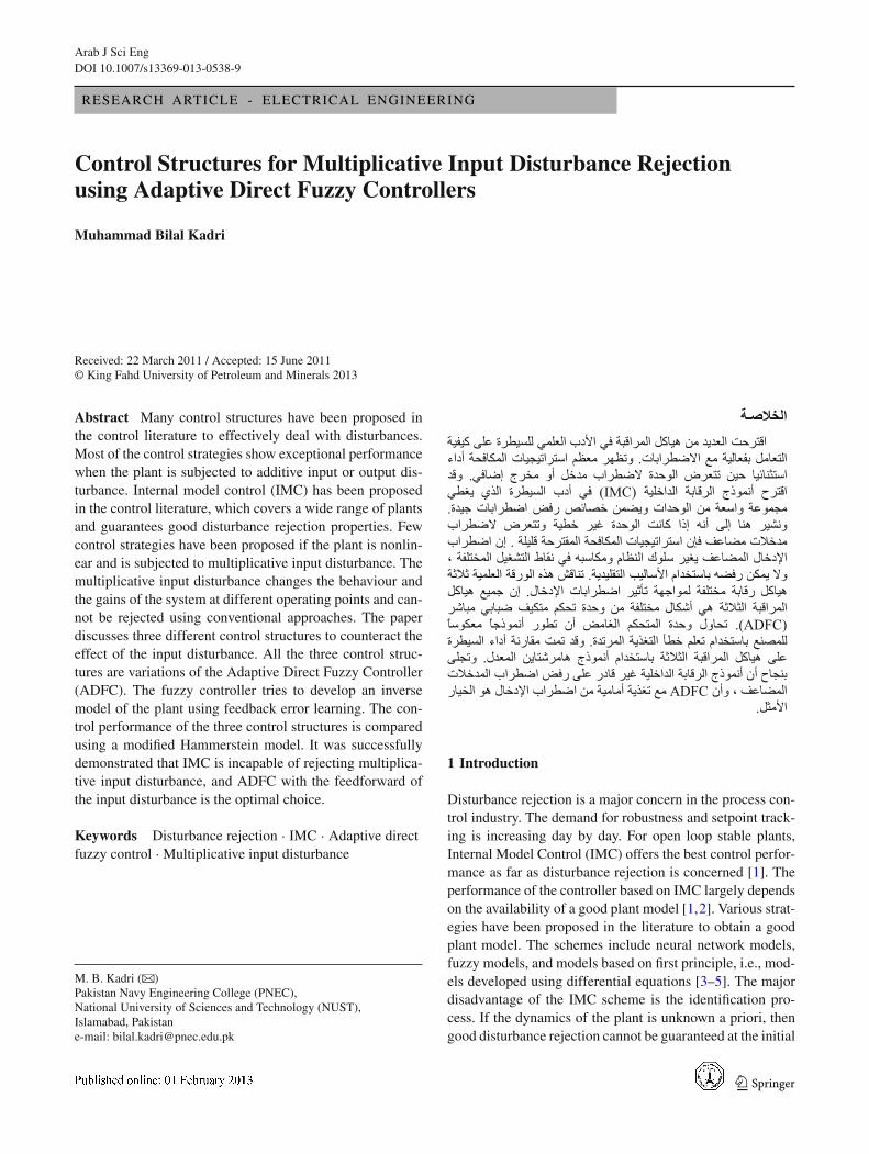
Fig. 2 ADFC without disturbance input (Control Scheme 1)
where ε(t) is the prediction error; uf(t) is the desired controlsignal which is calculated using ‘feedback error learning’law. aT(t − td)w(t − 1) represents the control signal esti-mated ‘td’ samples before which resulted in the control errore(t). If the control error is large, the desired control signalwill be large and consequently ε(t) will be big. The ε(t)will make a proportional change in rectifying the controllerparameters, i.e., the weights.
3 Different Approaches for Input Disturbance Rejection
3.1 ADFC with Unmeasured Disturbance(Control Scheme 1)
This basic control scheme, in which the controller has nodirect knowledge of the disturbance, is shown in Fig. 2. Thecontrol performance will be used as a benchmark for theother control schemes. The controller has feedback, whichwill reduce the effect of the disturbance, but it will not becompletely rejected.
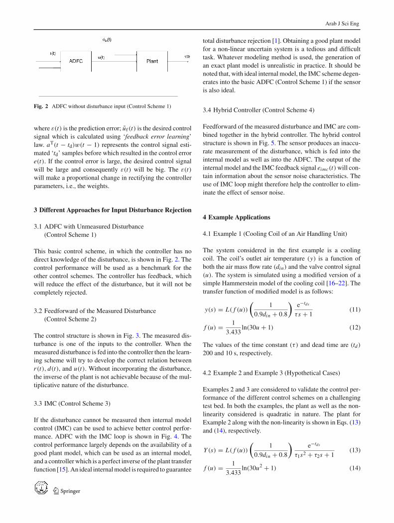
3.2 Feedforward of the Measured Disturbance(Control Scheme 2)
The control structure is shown in Fig. 3. The measured dis-turbance is one of the inputs to the controller. When themeasured disturbance is fed into the controller then the learn-ing scheme will try to develop the correct relation betweenr(t), d(t), and u(t). Without incorporating the disturbance,the inverse of the plant is not achievable because of the mul-tiplicative nature of the disturbance.
3.3 IMC (Control Scheme 3)
If the disturbance cannot be measured then internal modelcontrol (IMC) can be used to achieve better control perfor-mance. ADFC with the IMC loop is shown in Fig. 4. Thecontrol performance largely depends on the availability of agood plant model, which can be used as an internal model,and a controller which is a perfect inverse of the plant transferfunction [15]. An ideal internal model is required to guarantee
total disturbance rejection [1]. Obtaining a good plant modelfor a non-linear uncertain system is a tedious and difficulttask. Whatever modeling method is used, the generation ofan exact plant model is unrealistic in practice. It should benoted that, with ideal internal model, the IMC scheme degen-erates into the basic ADFC (Control Scheme 1) if the sensoris also ideal.
3.4 Hybrid Controller (Control Scheme 4)
Feedforward of the measured disturbance and IMC are com-bined together in the hybrid controller. The hybrid controlstructure is shown in Fig. 5. The sensor produces an inaccu-rate measurement of the disturbance, which is fed into theinternal model as well as into the ADFC. The output of theinternal model and the IMC feedback signal eimc(t) will con-tain information about the sensor noise characteristics. Theuse of IMC loop might therefore help the controller to elim-inate the effect of sensor noise.
4 Example Applications
4.1 Example 1 (Cooling Coil of an Air Handling Unit)
The system considered in the first example is a coolingcoil. The coil’s outlet air temperature (y) is a function ofboth the air mass flow rate (din) and the valve control signal(u). The system is simulated using a modified version of asimple Hammerstein model of the cooling coil [16–22]. Thetransfer function of modified model is as follows:
y(s) = L( f (u))
(1
0.9din + 0.8
)e−tds
τ s + 1(11)
f (u) = 1
3.433ln(30u + 1) (12)
The values of the time constant (τ ) and dead time are (td)
200 and 10 s, respectively.
4.2 Example 2 and Example 3 (Hypothetical Cases)
Examples 2 and 3 are considered to validate the control per-formance of the different control schemes on a challengingtest bed. In both the examples, the plant as well as the non-linearity considered is quadratic in nature. The plant forExample 2 along with the non-linearity is shown in Eqs. (13)and (14), respectively.
Y (s) = L( f (u))
(1
0.9din + 0.8
)e−tds
τ1s2 + τ2s + 1(13)
f (u) = 1
3.433ln(30u2 + 1) (14)
123
Arab J Sci Eng
Fig. 3 Feedforward of themeasured disturbance(Control Scheme 2)
Fig. 4 Disturbance rejectionusing neurofuzzy control withIMC (Control Scheme 3)
Fig. 5 Hybrid controller(Control Scheme 4)
The plant for Example 3 is given in Eqs. (15) and (16),respectively.
Y (s) = L( f (u))
(1
0.9din+ 0.8
)e−tds
τ1s2 + τ2s + 1(15)
f (u) = 1
11.7923[ln(30u + 1)]2 (16)
All the controller parameters are kept constant as inthe first example. τ1 and τ2 have values 200 and 100 s,respectively.
123
Arab J Sci Eng
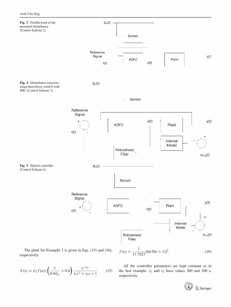
Fig. 6 Control performancewith unmeasured disturbance(Control Scheme 1)
Final control performance of Control Structure 1 with Plant 2
4.3 Experimental Setup
The value of the update rate (δ) for FLMS is 0.01. A 0thorder TS model is used to model the fuzzy controller. Feed-back error learning with a learning rate (γ ) of 0.5 is used. TheF-array values are initialized to zero and all of the rule conse-quents are initialized to 0.5. Input to the controller is x(t) =[r(t + td), y(t), d(t)] depending on the control structure. Allthe inputs have five membership functions with apexes at0.0, 0.25, . . . , 1.0. The reference model has a time constantof 200 s. The disturbance (din) is a sinusoid with a timeperiod of 900 s. The peak values of the (un-normalized) dis-turbance are 0.0 and 0.2. The disturbance is normalized so asto coincide with the apex of the membership functions. Thereis no output disturbance. The sensor noise is uniformly dis-tributed. The standard deviation of the noise is 0.8 and thesensor bias is 0.05. The sensor time constant is 300 s. Thetime constant of the IMC’s robustness filter is 200 s.
The normalized set-point is varied between 0 and 1 with astep size of 0.25, i.e., the set-point changes in the followingsequence: 0.0, 0.25, 0.50, 0.75, and 1.0.
5 Control Performance
The closed-loop behaviour when using the basic ADFC(Control Scheme 1) with both the plants is shown in Fig. 6. Itcan be seen that the basic ADFC is unable to reject the distur-bance satisfactorily especially when the plant is operating atvalues above 0.5. The effect of the sinusoidal disturbance canbe observed at levels 0.75 and 1, respectively. The closed-
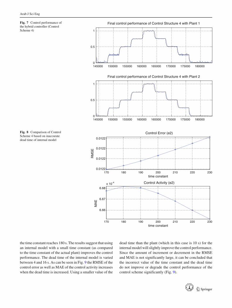
loop behaviour when using hybrid control scheme (ControlStructure 4) is shown in Fig. 7. In this case, the impact ofthe measurement noise is clearly visible on the plant output.Hybrid control scheme effectively rejects the disturbance atall operating points.
In Control Scheme 4, an ideal internal model is used. Thehybrid controller has reduced the impact of disturbance to agreater extent than Control Scheme 1. One of the objectivesof the hybrid scheme was to lessen the impact of the noisymeasurement. However, the effect of the noisy measurementis obvious in the controlled output. Nonetheless, there areimprovements in the RMSE of the control error as comparedto other control schemes.
6 Impact of Inaccurate Internal Model on the ControlPerformance
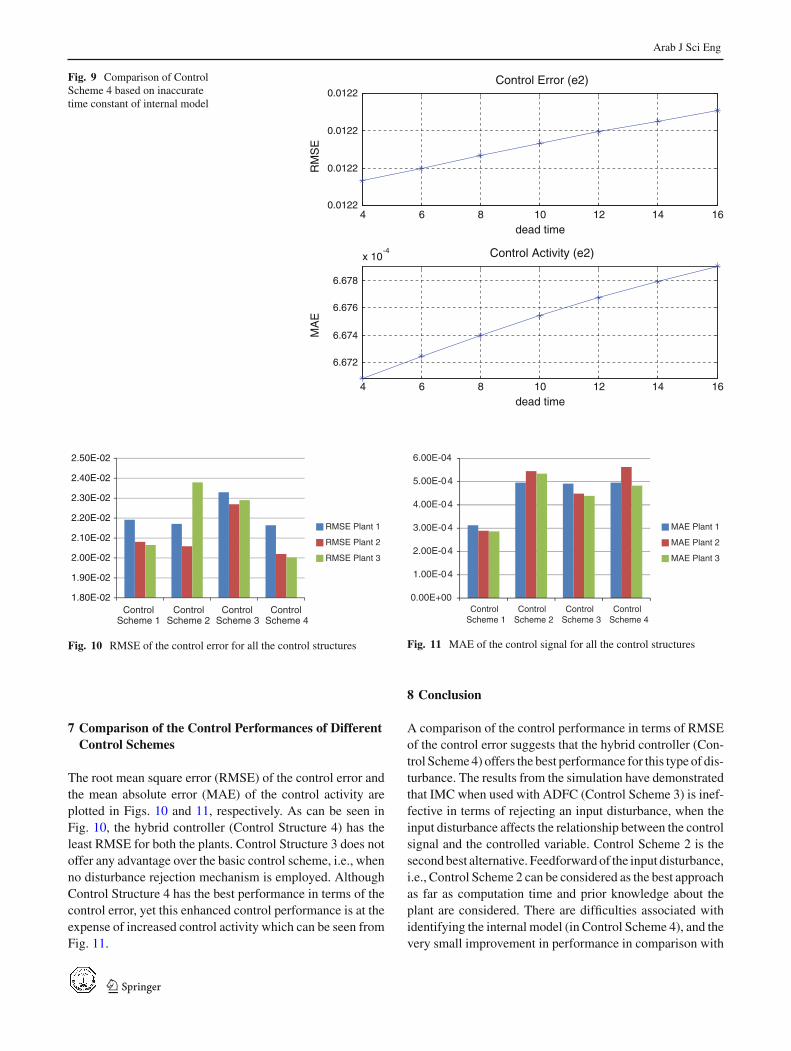
To determine the impact of an inaccurate internal model onthe control performance of the hybrid controller, the parame-ters (time constant and dead time of the Hammerstein model)of the internal model are varied. The RMSE of the controlerror and the MAE of the control activity are plotted for arange of values of the plant parameters. All the comparisonsare made when the ADFC has learnt and the initial transientshave died away. The time constant of the internal model isvaried between 170 and 230 s. The relationship of the con-trol performance with the time constant is shown in Fig. 8.The control error RMSE increases with the increasing valueof the time constant. On the contrary, the control activityincreases with the time constant but starts to decrease when
123
Arab J Sci Eng
Fig. 7 Control performance ofthe hybrid controller (ControlScheme 4)
Final control performance of Control Structure 4 with Plant 2
Fig. 8 Comparison of ControlScheme 4 based on inaccuratedead time of internal model
170 180 190 200 210 220 2300.0122
0.0122
0.0122
0.0122
time constant
RM
SE
Control Error (e2)
170 180 190 200 210 220 230
6.66
6.67
6.68x 10⁻⁴
time constant
MA
E
Control Activity (e2)
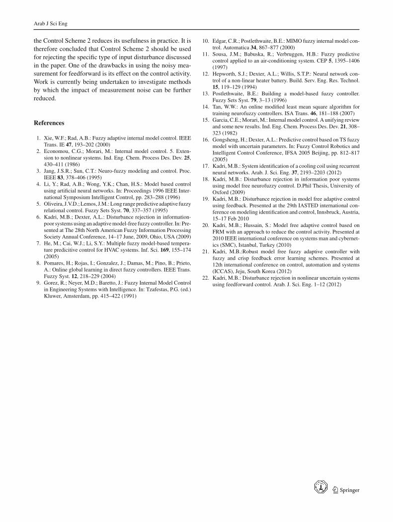
the time constant reaches 180 s. The results suggest that usingan internal model with a small time constant (as comparedto the time constant of the actual plant) improves the controlperformance. The dead time of the internal model is variedbetween 4 and 16 s. As can be seen in Fig. 9 the RMSE of thecontrol error as well as MAE of the control activity increaseswhen the dead time is increased. Using a smaller value of the
dead time than the plant (which in this case is 10 s) for theinternal model will slightly improve the control performance.Since the amount of increment or decrement in the RMSEand MAE is not significantly large, it can be concluded thatthe incorrect value of the time constant and the dead timedo not improve or degrade the control performance of thecontrol scheme significantly (Fig. 9).
123
Arab J Sci Eng
Fig. 9 Comparison of ControlScheme 4 based on inaccuratetime constant of internal model
4 6 8 10 12 14 160.0122
0.0122
0.0122
0.0122
dead time
RM
SE
Control Error (e2)
4 6 8 10 12 14 16
6.672
6.674
6.676
6.678
x 10-4
dead time
MA
E
Control Activity (e2)
1.80E-02
1.90E-02
2.00E-02
2.10E-02
2.20E-02
2.30E-02
2.40E-02
2.50E-02
ControlScheme 1
ControlScheme 2
ControlScheme 3
ControlScheme 4
RMSE Plant 1
RMSE Plant 2
RMSE Plant 3
Fig. 10 RMSE of the control error for all the control structures
7 Comparison of the Control Performances of DifferentControl Schemes
The root mean square error (RMSE) of the control error andthe mean absolute error (MAE) of the control activity areplotted in Figs. 10 and 11, respectively. As can be seen inFig. 10, the hybrid controller (Control Structure 4) has theleast RMSE for both the plants. Control Structure 3 does notoffer any advantage over the basic control scheme, i.e., whenno disturbance rejection mechanism is employed. AlthoughControl Structure 4 has the best performance in terms of thecontrol error, yet this enhanced control performance is at theexpense of increased control activity which can be seen fromFig. 11.
0.00E+00
1.00E-04
2.00E-04
3.00E-04
4.00E-04
5.00E-04
6.00E-04
ControlScheme 1
ControlScheme 2
ControlScheme 3
ControlScheme 4
MAE Plant 1
MAE Plant 2
MAE Plant 3
Fig. 11 MAE of the control signal for all the control structures
8 Conclusion
A comparison of the control performance in terms of RMSEof the control error suggests that the hybrid controller (Con-trol Scheme 4) offers the best performance for this type of dis-turbance. The results from the simulation have demonstratedthat IMC when used with ADFC (Control Scheme 3) is inef-fective in terms of rejecting an input disturbance, when theinput disturbance affects the relationship between the controlsignal and the controlled variable. Control Scheme 2 is thesecond best alternative. Feedforward of the input disturbance,i.e., Control Scheme 2 can be considered as the best approachas far as computation time and prior knowledge about theplant are considered. There are difficulties associated withidentifying the internal model (in Control Scheme 4), and thevery small improvement in performance in comparison with
123
Arab J Sci Eng
the Control Scheme 2 reduces its usefulness in practice. It istherefore concluded that Control Scheme 2 should be usedfor rejecting the specific type of input disturbance discussedin the paper. One of the drawbacks in using the noisy mea-surement for feedforward is its effect on the control activity.Work is currently being undertaken to investigate methodsby which the impact of measurement noise can be furtherreduced.
4. Li, Y.; Rad, A.B.; Wong, Y.K.; Chan, H.S.: Model based controlusing artificial neural networks. In: Proceedings 1996 IEEE Inter-national Symposium Intelligent Control, pp. 283–288 (1996)
5. Oliveira, J.V.D.; Lemos, J.M.: Long range predictive adaptive fuzzyrelational control. Fuzzy Sets Syst. 70, 337–357 (1995)
6. Kadri, M.B.; Dexter, A.L.: Disturbance rejection in information-poor systems using an adaptive model-free fuzzy controller. In: Pre-sented at The 28th North American Fuzzy Information ProcessingSociety Annual Conference, 14–17 June, 2009, Ohio, USA (2009)
7. He, M.; Cai, W.J.; Li, S.Y.: Multiple fuzzy model-based tempera-ture predicitive control for HVAC systems. Inf. Sci. 169, 155–174(2005)
8. Pomares, H.; Rojas, I.; Gonzalez, J.; Damas, M.; Pino, B.; Prieto,A.: Online global learning in direct fuzzy controllers. IEEE Trans.Fuzzy Syst. 12, 218–229 (2004)
9. Gorez, R.; Neyer, M.D.; Baretto, J.: Fuzzy Internal Model Controlin Engineering Systems with Intelligence. In: Tzafestas, P.G. (ed.)Kluwer, Amsterdam, pp. 415–422 (1991)
10. Edgar, C.R.; Postlethwaite, B.E.: MIMO fuzzy internal model con-trol. Automatica 34, 867–877 (2000)
11. Sousa, J.M.; Babuska, R.; Verbruggen, H.B.: Fuzzy predictivecontrol applied to an air-conditioning system. CEP 5, 1395–1406(1997)
13. Postlethwaite, B.E.: Building a model-based fuzzy controller.Fuzzy Sets Syst. 79, 3–13 (1996)
14. Tan, W.W.: An online modified least mean square algorithm fortraining neurofuzzy controllers. ISA Trans. 46, 181–188 (2007)
15. Garcia, C.E.; Morari, M.: Internal model control. A unifying reviewand some new results. Ind. Eng. Chem. Process Des. Dev. 21, 308–323 (1982)
16. Gongsheng, H.; Dexter, A.L.: Predictive control based on TS fuzzymodel with uncertain parameters. In: Fuzzy Control Robotics andIntelligent Control Conference, IFSA 2005 Beijing, pp. 812–817(2005)
17. Kadri, M.B.: System identification of a cooling coil using recurrentneural networks. Arab. J. Sci. Eng. 37, 2193–2203 (2012)
18. Kadri, M.B.: Disturbance rejection in information poor systemsusing model free neurofuzzy control. D.Phil Thesis, University ofOxford (2009)
19. Kadri, M.B.: Disturbance rejection in model free adaptive controlusing feedback. Presented at the 29th IASTED international con-ference on modeling identification and control, Innsbruck, Austria,15–17 Feb 2010
20. Kadri, M.B.; Hussain, S.: Model free adaptive control based onFRM with an approach to reduce the control activity. Presented at2010 IEEE international conference on systems man and cybernet-ics (SMC), Istanbul, Turkey (2010)
21. Kadri, M.B.:Robust model free fuzzy adaptive controller withfuzzy and crisp feedback error learning schemes. Presented at12th international conference on control, automation and systems(ICCAS), Jeju, South Korea (2012)
22. Kadri, M.B.: Disturbance rejection in nonlinear uncertain systemsusing feedforward control. Arab. J. Sci. Eng. 1–12 (2012)