Page 1
CONTROL SYSTEM DESIGN FOR A HAPTIC DEVICE
A THESIS SUBMITTED TO THE GRADUATE SCHOOL OF NATURAL AND APPLIED SCIENCES
OF MIDDLE EAST TECHNICAL UNIVERSITY
BY
SÜLEYMAN BİDECİ
IN PARTIAL FULFILLMENT OF THE REQUIREMENTS FOR
THE DEGREE OF MASTER OF SCIENCE IN
MECHANICAL ENGINEERING DEPARTMENT
SEPTEMBER 2007
Page 2
Approval of the thesis
“CONTROL SYSTEM DESIGN FOR A HAPTIC DEVICE”
Submitted by SÜLEYMAN BİDECİ in partial fulfillment of the requirements for the degree of Master of Science in Mechanical Engineering Department, Middle East Technical University by, Prof. Dr. Canan Özgen _____________________ Dean, Graduate School of Natural and Applied Sciences Prof. Dr. Kemal İder _____________________ Head of Department, Mechanical Engineering Assist. Prof. Dr. İlhan Konukseven _____________________ Supervisor, Mechanical Engineering Dept., METU Examining Committee Members: Prof. Dr. Reşit Soylu _____________________ Mechanical Engineering Dept., METU Assist. Prof. Dr. İlhan Konukseven _____________________ Mechanical Engineering Dept., METU Assoc. Prof. Dr. Veysel Gazi _____________________ Electrical Engineering Dept., TOBB Assist. Prof. Dr. Buğra Koku _____________________ Mechanical Engineering Dept., METU Assist. Prof. Dr. Yiğit Yazıcıoğlu _____________________ Mechanical Engineering Dept., METU
Date: 07 / 09 / 2007
Page 3
iii
I hereby declare that all information in this document has been obtained and
presented in accordance with academic rules and ethical conduct. I also declare
that, as requires by thesis rules and conduct, I have fully cited and referenced
all material and results that are not original to this work.
Name, Last Name : Süleyman Bideci
Signature :
Page 4
iv
ABSTRACT
CONTROL SYSTEM DESIGN FOR A HAPTIC DEVICE
Bideci, Süleyman
M.S. Department of Mechanical Engineering
Supervisor: Asst. Prof. Dr. E. İlhan Konukseven
September 2007, 108 Pages
In this thesis, development of a control system is aimed for a 1 DOF haptic device,
namely Haptic Box. Besides, it is also constructed. Haptic devices are the
manipulators that reflect the interaction forces with virtual or remote environments to
its users. In order to reflect stiffness, damping and inertial forces on a haptic device
position, velocity and acceleration measurements are required. The only motion
sensor in the system is an incremental optical encoder attached to the back of the DC
motor. The encoder is a good position sensor but velocity and acceleration
estimations from discrete position and time data is a challenging work. To estimate
velocity and acceleration some methods in the literature are employed on the Haptic
Box and it is concluded that Kalman filtering gives the best results. After the velocity
and acceleration estimations are acquired haptic control algorithms are tried
experimentally. Finally, a virtual environment application is presented.
Keywords: haptic control, velocity estimation, acceleration estimation, Kalman Filter
Page 5
v
ÖZ
BİR HAPTİK CİHAZ İÇİN KONTROL SİSTEMİ TASARIMI
Bideci, Süleyman
Yüksek Lisans, Makina Mühendisliği Bölümü
Tez Yöneticisi: Yrd. Doç. Dr. E. İlhan Konukseven
Eylül 2007, 108 Sayfa
Bu tezde, Heptik Kutu isimli, tek serbestlik dereceli bir heptik cihaz için kontrol
sistemi geliştirilmesi amaçlanmıştır. Ayrıca, Heptik Kutu bu çalışma kapsamında
oluşturulmuştur. Heptik cihazlar sanal yada uzak ortamlardaki etkileşim kuvvetlerini
kullanıcıya yansıtan manipülatörlerdir. Sertlik, sönümleme ve atalet kuvvetlerini
heptik cihaza yansıtmak için konum, hız ve ivme ölçümüne ihtiyaç vardır.
Sistemdeki tek hareket algılayıcısı DC motorun arkasına takılı olan optik bir artırımlı
kodlayıcıdır. Artırımlı kodlayıcılar iyi konum algılayıcılarıdır fakat kesikli konum ve
zaman bilgisinden hız ve ivme tahmini zor bir iştir. Hız ve ivme tahmini için
literatürdeki bazı metotlar Heptik Kutu üzerinde denenmiş ve Kalman filtrelemesinin
en iyi sonucu verdiği görülmüştür. Hız ve ivme bilgisi elde edildikten sonra deneysel
olarak heptik algoritmaları denenmiştir. Son olarak bir sanal ortam uygulaması
yapılmıştır.
Anahtar Kelimeler : heptik kontrol, hız tahmini, ivme tahmini, Kalman Filtresi
Page 7
vii
ACKNOWLEDGMENT
I would like to thank my thesis supervisor Asst. Prof. Dr. E. İlhan Konukseven for
providing me this research opportunity, and guiding me through the study.
I owe special thanks to Asst. Prof. Dr. Uluç Saranlı from Department of Computer
Engineering, Bilkent University for his invaluable help to construct the Haptic Box,
and for his support.
I would like to express my gratitude to Özgür Cavbozar, Arda Özgen, Hüseyin
Öztürk and Halit Şahin who are the staff of METU BILTIR – CAD/CAM and
Robotics Center.
I thank to my friends Anas Abidi, Emre Sezginalp, Faruk Yazıcıoğlu, Onur
Yarkınoğlu, Umut Koçak and Varlık Kılıç who studied in the METU Mechatronics
Laboratory for their precious support and presence.
Finally, I am deeply grateful to my very dear family, especially my parents, for
supporting me and for showing me love to carry on my work successfully.
Page 8
viii
TABLE OF CONTENTS
ABSTRACT ........................................................................................................... iv
ÖZ ............................................................................................................................v
ACKNOWLEDGMENT........................................................................................ vii
TABLE OF CONTENTS...................................................................................... viii
LIST OF SYMBOLS ............................................................................................ xiii
CHAPTERS
1. INTRODUCTION ............................................................................................1
1.1 Introduction.................................................................................................1
1.2 Objectives of the Thesis ..............................................................................3
1.3 Thesis Outline .............................................................................................3
2. HAPTIC DEVICES ..........................................................................................4
2.1 Some Commercial Haptic Devices ..............................................................5
2.2 Haptic Applications.....................................................................................7
3. HAPTIC BOX.................................................................................................11
3.1 Haptic Box Specifications .........................................................................12
3.1.1 Copley 413CE DC Brush Servo Amplifier..............................................13
3.1.2 Maxon RE40 DC Motor and Optical Incremental Encoders ................13
3.1.3 Other Components..............................................................................13
4. HAPTIC CONTROL ......................................................................................15
4.1 Impedance & Admittance ..........................................................................16
4.2 Robot Control............................................................................................17
4.3 Haptic Control...........................................................................................20
4.3.1 Impedance Control .............................................................................20
4.3.2 Admittance Control ............................................................................22
4.3.3 Haptic Control Conclusions ................................................................24
Page 9
ix
5. VELOCITY AND ACCELERATION ESTIMATION ....................................25
5.1 Velocity Estimation Methods in Literature ................................................26
5.2 Velocity Estimation Algorithms ................................................................27
5.2.1 Fixed-time Velocity Estimation ..........................................................28
5.2.2 Fixed-position Velocity Estimation.....................................................29
5.2.3 Combined and Adaptive Velocity Estimation Algorithms ...................30
5.2.4 Velocity and Acceleration Estimation with Kalman Filters .................34
6. SYSTEM IMPLEMENTATION.....................................................................38
6.1 Experiment Setup ......................................................................................38
6.2 Velocity and Acceleration Estimations ......................................................40
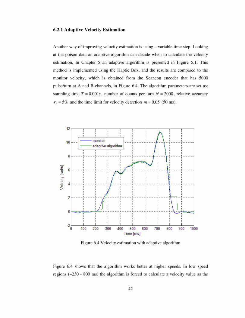
6.2.1 Adaptive Velocity Estimation .............................................................42
6.2.2 Velocity Estimation with Kalman Filters ............................................43
6.3 Control System Applications .....................................................................48
6.4.1 Open Loop Impedance Control ...........................................................52
6.4.2 Impedance Control with Force-feedback.............................................53
6.4.3 Admittance Control ............................................................................54
6.4 Case Study ................................................................................................55
7. CONCLUSION...............................................................................................58
7.1 Conclusions...............................................................................................58
7.2 Future Work..............................................................................................59
REFERENCES .......................................................................................................60
APPENDICES
A. KALMAN FILTER CODE FOR CONSTANT VELOCITY MODEL............64
B. HAPTIC BOX COMPONENTS AND EXPERIMENTAL MATERIALS ......66
C. HAPTIC INTERFACE ELECTRICAL CONNECTIONS ..............................72
D. HAPTIC BOX TECHNICAL DRAWINGS ...................................................75
E. SIMULINK BLOCK DETAILS USED IN EXPERIMENTS........................104
E.1 Open Loop Impedance Control ...............................................................105
E.2 Impedance Control with Force Feed-back ...............................................106
E.3 Admittance Control.................................................................................107
Page 10
x
LIST OF FIGURES
Figure 1.1 Haptic Box...............................................................................................2
Figure 2.1 PHANTOM Premium 1.5/6 DOF Haptic Device......................................5
Figure 2.2 The CyberGrasp.......................................................................................6
Figure 2.3 Delta 3DOF and Omega.3 ........................................................................6
Figure 2.4 a) Virtual Clay b) Virtual Sculpting..........................................................8
Figure 2.5 Haptic Painting brush models...................................................................8
Figure 2.6 a) Virtual Painting Application b) Virtual Painting...................................9
Figure 2.7 Teleoperation employing a haptic device................................................10
Figure 3.1 Haptic Box.............................................................................................11
Figure 3.2 Haptic Box Components ........................................................................12
Figure 4.1 Force based explicit force control...........................................................18
Figure 4.2 Position based explicit force control.......................................................19
Figure 4.3 Impedance control with force feedback ..................................................19
Figure 4.4 Impedance control with force feedback and model feed forward ............21
Figure 4.5 Open Loop Impedance Control with model feed forward .......................22
Figure 4.6 Admittance Control................................................................................23
Figure.5.1 The velocity estimation algorithm proposed in [4]..................................33
Figure 5.2 Recursive Prediction-Correction Structure of the Kalman Filter .............37
Figure 6.1 Haptic Interface......................................................................................39
Figure 6.2 Effect of discretization on velocity estimation in low velocity region .....41
Figure 6.3 CET Method ..........................................................................................41
Figure 6.4 Velocity estimation with adaptive algorithm ..........................................42
Figure 6.5 Velocity Estimation with Kalman Filter – Constant Velocity model .......44
Figure 6.6 Velocity Est. – Kalman Filter Const. Acc. – Low Velocity Region.........46
Figure 6.7 Velocity Est. – Kalman Filter Const. Acc. – High Velocity Region ........47
Figure 6.8 Acceleration estimation with Kalman Filter – Constant Acc. Model.......48
Figure 6.9 Transducer output voltage & torque input relation..................................49
Figure 6.10 Copley 413CE reference voltage & output current relation...................50
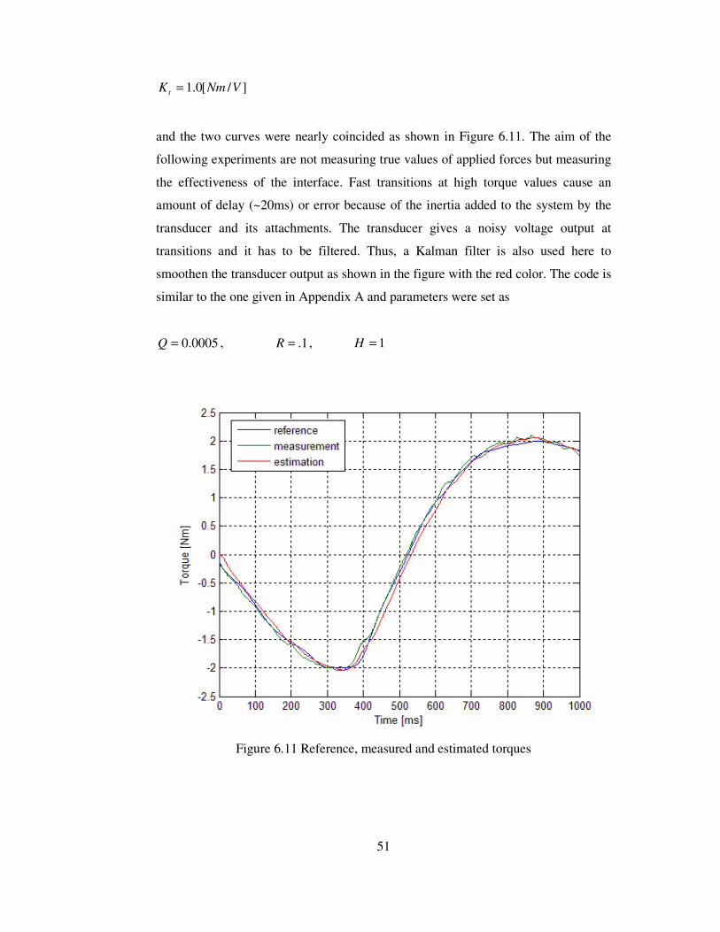
Figure 6.11 Reference, measured and estimated torques..........................................51
Figure 6.12 Simulink model of open loop impedance control ..................................52
Figure 6.13 Impedance control with force-feed back ...............................................54
Page 11
xi
Figure 6.14 Admittance Control..............................................................................54
Figure 6.15 Simulated Virtual Environment ............................................................56
Figure B.1 Maxon RE40 DC Brushes Motor Specifications ....................................67
Figure B.2 Scancon Encoder Specifications ............................................................68
Figure B.3 Copley 413CE Servo Amplifier .............................................................69
Figure B.4 HEDS 5540A Encoder...........................................................................69
Figure B.5 NI PCI6052E Multifunction DAQ .........................................................70
Figure B.6 NI PCI6602 Counter/Timer DAQ..........................................................70
Figure B.7 W.M.Berg Sprocket Gear ......................................................................71
Figure B.8 W.M.Berg Polyurethane/Steel Cable Chain ...........................................71
Figure C.1 Electrical connections inside the Haptic Box .........................................73
Figure C.2 Electrical connections between Haptic Box and Target Computer.........73
Figure C.3 Configuration for Copley 413CE Servo Amplifier .................................74
Figure D.1 Vertical Plate Front ...............................................................................76
Figure D.2 Vertical Plate Back................................................................................77
Figure D.3 Vertical Plate Middle ............................................................................78
Figure D.4 Horizontal Plate ....................................................................................79
Figure D.5 Top Wall...............................................................................................80
Figure D.6 Left Wall...............................................................................................81
Figure D.7 Front Wall.............................................................................................82
Figure D.8 Back Wall .............................................................................................83
Figure D.9 Right Wall.............................................................................................84
Figure D.10 Connector Block Sidewall ...................................................................85
Figure D.11 Connector Block Backwall ..................................................................86
Figure D.12 Cable Stand.........................................................................................87
Figure D.13 Motor Holding Plate............................................................................88
Figure D.14 PinD5 & Disk Bracket.........................................................................89
Figure D.15 Outer Cylinder ....................................................................................90
Figure D.16 Handle Shaft V3.0...............................................................................91
Figure D.17 Knob ...................................................................................................92
Figure D.18 Knob Neck ..........................................................................................93
Figure D.19 Handle Shaft V4.0...............................................................................94
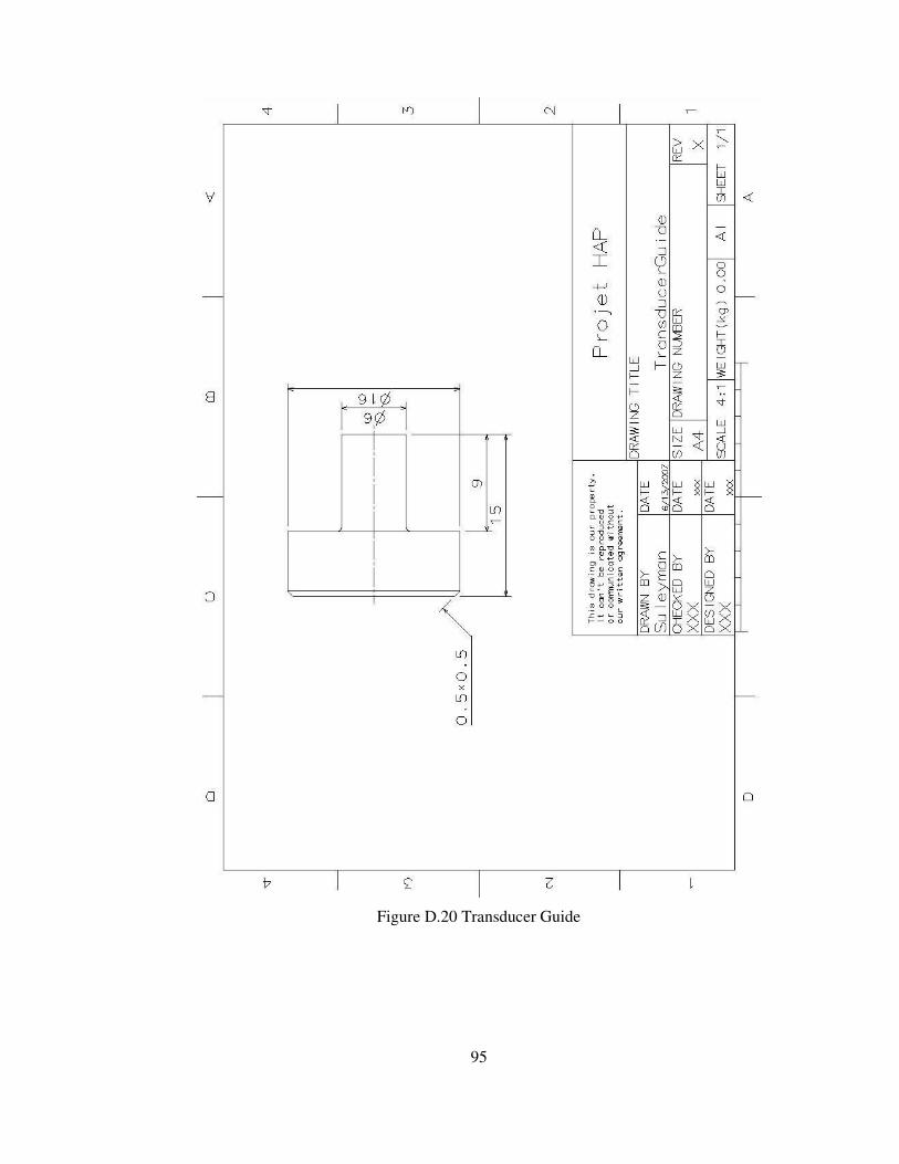
Figure D.20 Transducer Guide ................................................................................95
Page 12
xii
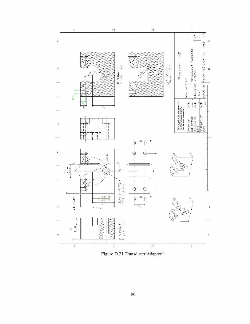
Figure D.21 Transducer Adaptor 1..........................................................................96
Figure D.22 Transducer Adaptor 3..........................................................................97
Figure D.23 Motor Holding Product V3.0 ...............................................................98
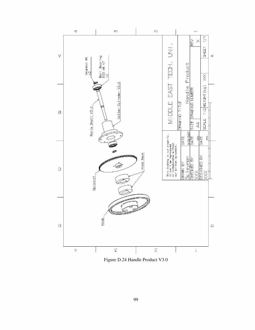
Figure D.24 Handle Product V3.0 ...........................................................................99
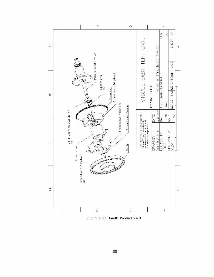
Figure D.25 Handle Product V4.0 .........................................................................100
Figure D.26 Main Frame.......................................................................................101
Figure D.27 Cover ................................................................................................102
Figure D.28 Haptic Box ........................................................................................103
Figure E.1 Virtual Environment Model Block.......................................................105
Figure E.2 Haptic Box Block ................................................................................105
Figure E.3 Controller Block ..................................................................................105
Figure E.4 Virtual Environment Block..................................................................106
Figure E.5 Controller Block ..................................................................................106
Figure E.6 Copley Parameters Block.....................................................................106
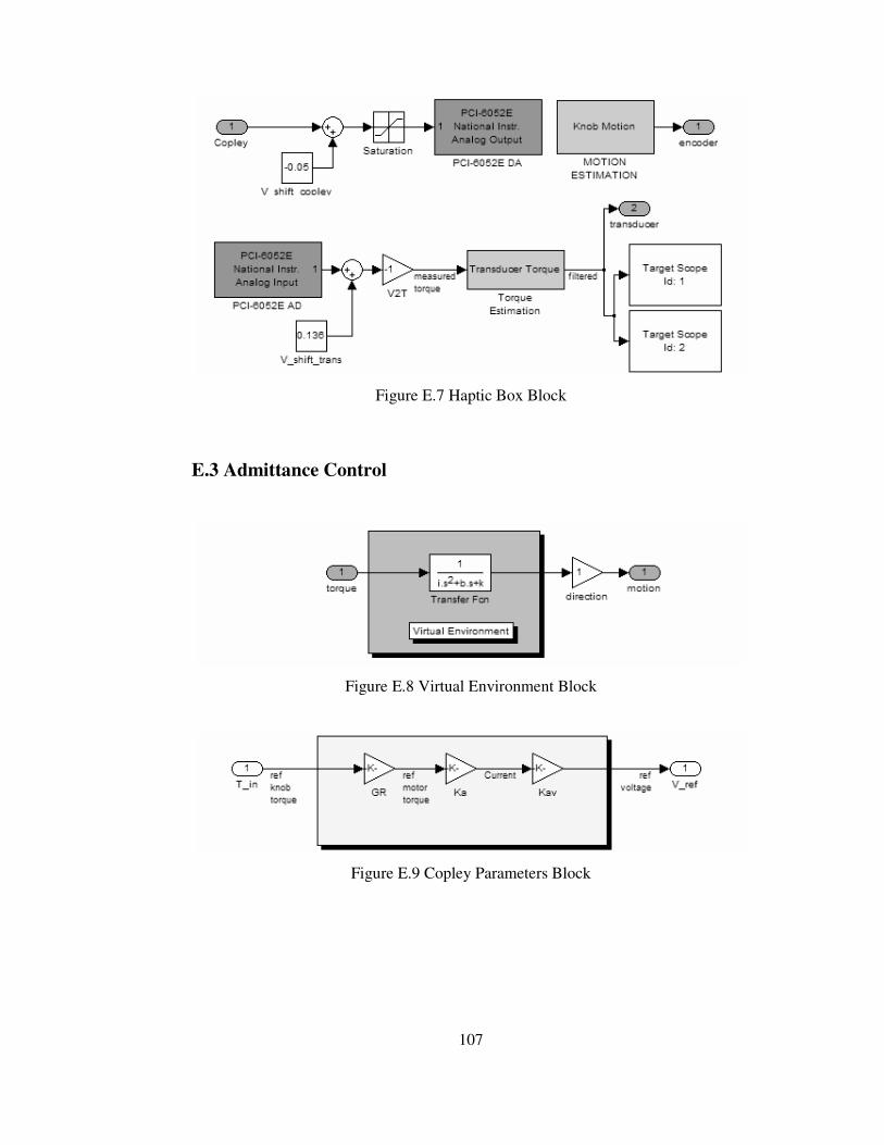
Figure E.7 Haptic Box Block ................................................................................107
Figure E.8 Virtual Environment Block..................................................................107
Figure E.9 Copley Parameters Block.....................................................................107
Figure E.10 Controller Block ................................................................................108
Figure E.11 Haptic Box Block ..............................................................................108
Page 13
xiii
LIST OF SYMBOLS
Z Impedance
1−Z Admittance
J Jacobian Matrix
N Number of lines per encoder channel
T Sampling period
f Generalized force
x& Generalized motion
υ Velocity
elT Elapsed time
eR Encoder resolution
θ Angular position
jr Relative accuracy
X State matrix
X Estimated state matrix
K Kalman gain matrix
φ State transition matrix
ψ State input matrix
Y Measurement matrix
P Estimated variance matrix
R Variance matrix of the measurement noise
Q Variance matrix of the system noise
H Measured values matrix
tK Transducer torque-voltage constant
avK Servo amplifier current-voltage constant
aK Motor torque constant
k Stiffness constant
b Damping constant
i One dimensional inertia constant
pK Proportional controller gain
Page 14
1
CHAPTER 1
INTRODUCTION
1.1 Introduction
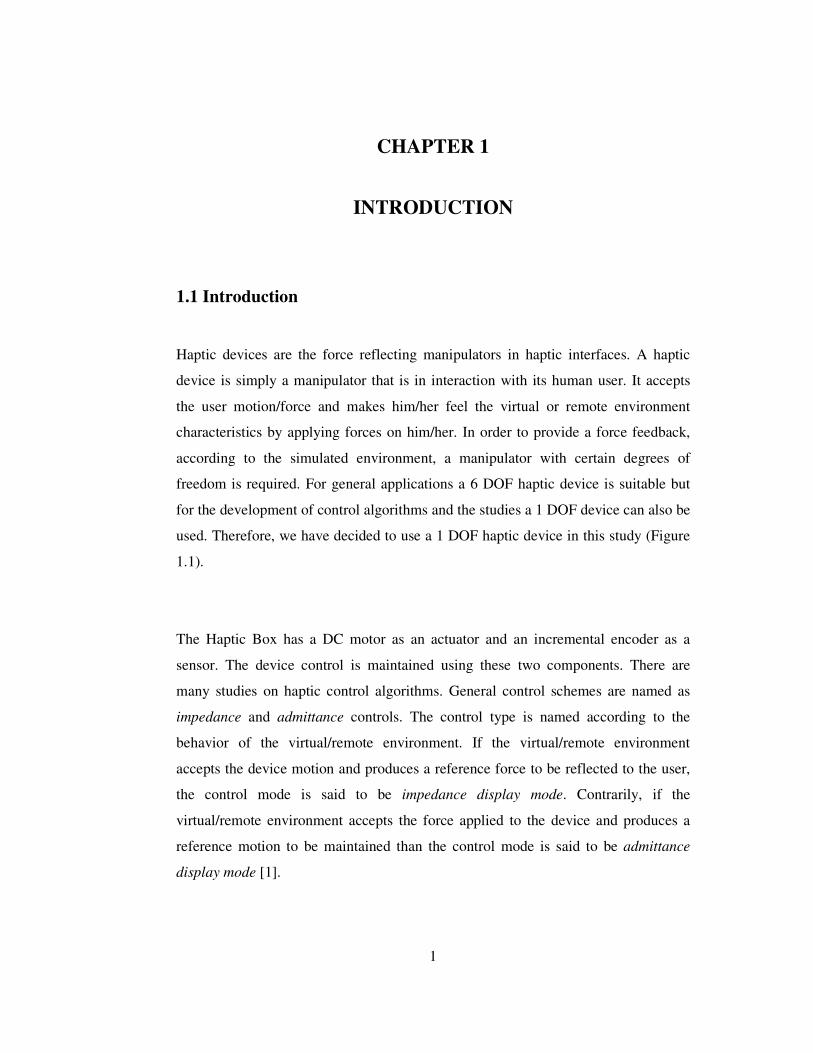
Haptic devices are the force reflecting manipulators in haptic interfaces. A haptic
device is simply a manipulator that is in interaction with its human user. It accepts
the user motion/force and makes him/her feel the virtual or remote environment
characteristics by applying forces on him/her. In order to provide a force feedback,
according to the simulated environment, a manipulator with certain degrees of
freedom is required. For general applications a 6 DOF haptic device is suitable but
for the development of control algorithms and the studies a 1 DOF device can also be
used. Therefore, we have decided to use a 1 DOF haptic device in this study (Figure
1.1).
The Haptic Box has a DC motor as an actuator and an incremental encoder as a
sensor. The device control is maintained using these two components. There are
many studies on haptic control algorithms. General control schemes are named as
impedance and admittance controls. The control type is named according to the
behavior of the virtual/remote environment. If the virtual/remote environment
accepts the device motion and produces a reference force to be reflected to the user,
the control mode is said to be impedance display mode. Contrarily, if the
virtual/remote environment accepts the force applied to the device and produces a
reference motion to be maintained than the control mode is said to be admittance
display mode [1].
Page 15
2
Figure 1.1 Haptic Box
Whatever the type of the controller is, the control system requires the information
about the device motion. Position measurement is done via the incremental encoder
discretely and precisely but velocity and acceleration estimation from this discrete
data is not easy. Gathering accurate measurement/estimation data is another
important part of the control work and it determines the effectiveness of the haptic
interface. To estimate velocity from discrete position and time data, many methods
are proposed in the literature. Fixed time and fixed position velocity estimations are
two commonly used methods. To improve these estimators some other numerical
techniques such as use of Taylor series and backward expansions and curve fits are
used [2]. To decrease discretization errors counters for position and time are used
simultaneously in the CET method [3]. To detect velocities at various speeds
adaptive algorithms are proposed that allows the user to choose between relative
accuracy and time delay [4]. Some observer based estimators are used in [5]. Finally,
Kalman Filters are employed to estimate velocity from incremental encoder data
[6,7,8,9,10,11].
Page 16
3
1.2 Objectives of the Thesis
The first objective of this thesis is to develop a haptic device for experimental
applications. Next objective is to try haptic control algorithms on the developed
haptic device. Most of the haptic devices in the market do not have any force
feedback capability. The third objective of this thesis is to add force feedback
capability to the developed haptic device.
1.3 Thesis Outline
The study is arranged as, in Chapter 2 haptic devices are presented and some haptic
applications are described. The Haptic Box is explained in Chapter 3. In Chapter 4
haptic control schemes are described and velocity and acceleration estimation
methods are given in Chapter 5. System implementation using the Haptic Box is
expressed in Chapter 6 and conclusions are made in Chapter 7.
Page 17
4
CHAPTER 2
HAPTIC DEVICES
Manipulators have been used for a long time in industrial applications. They are
simply some mechanical devices simulating human motions to replace man
handwork with machine precision and speed. For example, robots in automotive
production lines are used for welding, drilling, part placement, etc., simulating
human arm motions. These manipulators are commanded by a computer which is
programmed by an operator. To control the device position and sometimes velocity,
encoders on the joints of the manipulators are used. For general industrial robot
applications, motion feedback is sufficient. However, for some others, the interaction
force between the robot and workpiece becomes very important as this force may
damage the workpiece or the manipulator. In these kind of applications force
transducers are used to measure the interaction force. Thereby, the force feedback
signal may be used to control the interaction force.
The way of using manipulators mentioned above requires a computer that is
programmed by an operator. The application is in the control of the computer. On the
other hand, in some applications human inspection becomes unavoidable. Hazardous
experiments can be given as an example. The operator grasps the objects using the
remote robot by visual information. As the user is not given any force information,
he/she does not know how hard he/she handles the objects. Another example can be
given in the area of Virtual Reality (VR). In VR operations 3D environments are
examined by stereo glasses and this gives the user only visual information. However,
besides the visual feedback from the virtual or remote environments, touching them
would be more impressive and this is possible with haptic devices. Thanks to haptic
devices touching those virtual and remote environments becomes possible. Ueberle
and Buss made a definition of haptic devices as “Haptic displays are force reflecting
Page 18
5
human system interfaces that are in physical contact with the operator providing
bidirectional interaction by sensing user motion and exerting forces on him/her.” [1].
As described in Chapter4 sensing motion for device control is not a single way to
render the contact force. Thus, the definition “Haptic displays aim to provide users
with a sense of touch, rendering contact forces as if interactions were occurring with
real objects.” made by Hwang, Williams and Niemeyer gives a more generic and
realistic explanation [12].
2.1 Some Commercial Haptic Devices
In recent days, use of haptic devices has become popular. Universities are developing
new haptic devices and some companies produce their products. Phantom Premium
1.5/6 DOF Haptic Device [13] from Sensable Technologies, Inc. shown in Figure 2.1
is one of those devices. It can apply force in three translational directions and torque
in three rotational directions.
Figure 2.1 PHANTOM Premium 1.5/6 DOF Haptic Device
Page 19
6
In Figure 2.2, The CyberGrasp[14] from Immersion Corporation is shown with an
application. This device allows the user feel the forces on his/her fingers.
Figure 2.2 The CyberGrasp
Figure 2.3 Delta 3DOF and Omega.3
Page 20
7
In essence haptic devices are some kind of mechanical manipulators with special
controlling units, so the manipulator type can vary. Delta 3DOF and Omega.3 [15]
shown in Figure 2.3 are haptic devices with parallel manipulators, which are from
Force Dimension Company. Parallel structures are preferred for high force
applications, thus these devices are used to reflect large forces in three translational
dimensions.
2.2 Haptic Applications
As described before, with haptic devices human motion can be simulated.
Considering this fact, any human work can be a haptic application; however, general
studies are on medicine, military, education and training, entertainment, CAD/CAM,
reverse engineering and art fields.
A simple and illustrative example is the CAD application given in Figure 2.2. Using
the CyberGrasp, the user assembles the nut and bolt. In this application, by the
operator motion the virtual objects are moved and also the user feels the forces on
his/her fingers as if he/she assembles a real nut and bolt pair.
Surgical trainings are another great application filed. Haptic interfaces are getting
used more at different medical operational simulations. New haptic devices
IOMaster7D and IOMaster5D are developed to apply to endoscopic neurosurgery,
ENT surgery and laparoscopy simulation [16].
There are some training simulators for some works requiring practice. Military and
medical operations can be given as examples. A medical application is examined in
[17] in which a tennis simulator is developed to examine human arm characteristics
from arm movement.
Page 21
8
Figure 2.4 a) Virtual Clay b) Virtual Sculpting
An interesting application area is field of art in which a haptic device takes place of
an art tool. Virtual sculpting and virtual painting are two good examples. In a virtual
sculpting operation virtual clay is used and it is deformed by the virtual tool (Fig.2.4a)
[18]. The virtual clay is modeled as a real one, such that, it is deformable, has
stiffness and damping properties. Thus, the user shapes it feeling realistic touch. In
Figure 2.4b, an application on human nose is shown. In this operation a spherical
virtual tool is used. The tools are interchangeable with different shapes so the tool
shape is taken into consideration at deformation stage.
Figure 2.5 Haptic Painting brush models
Page 22
9
Virtual painting is an application similar one to the virtual sculpting. However, the
deformation and forces are also calculated at the tool tip, namely that the brush head
is deformed at strokes. To reflect these properties to the user, brush models are made
as shown in Figure 2.5. In the figure, the column named structure is used for force
calculation and so the deformation, and visual models are given in the surface
column. The user uses the haptic device end-effector as the brush as shown in Figure
2.6a. And a sample painting made by a user of the system is shown in Figure 2.6b
[19].
Besides these virtual environment applications, there are some real world
applications, in which haptic devices are used. These kinds of applications are called
teleoperations. Teleoperations are important applications as they mostly serve to the
surgical operations. In these operations, the virtual environments are replaced by real
remote environments. This is also needed in hazardous experiments and in some
variety of applications where contact force is needed to be controlled by a human
operator. Such an application is shown in Figure 2.7. The ViSHARD10 is 10DOF
haptic device and it is called the master manipulator. And the 7DOF remote robot is
the slave one.
Figure 2.6 a) Virtual Painting Application b) Virtual Painting
Page 23
10
The slave robot copies the motion of the master one. The force sensors attached to
the slave robot contact forces sense the contact forces and transmit them to the
master robot, which is the haptic device. A stereo camera is also employed to gather
the visual information [20].
Figure 2.7 Teleoperation employing a haptic device
As is seen, haptic devices are playing important roles in many applications. They
take place in virtual environment applications for modeling some lost human parts to
manufacture prosthesis. They can be used to train students for surgical practices, art
students to gain experience, and in many computer games. In military field, it can be
used to reflect realistic forces in simulators. In telemanipulation applications they can
be employed to perform surgical operations and hazardous experiments.
The applicability to many simulations make haptic devices important. Thanks to
them lots of simulations can be done to gather information from different systems.
By this way, repeatability of experiments increases and as the used experimental set
up is virtual, experiment costs can be decreased if accurate system models can be
done. Effects of products can be estimated using virtual models before producing
them and damages of hazardous environments can be avoided with the help of haptic
interfaces.
Page 24
11
CHAPTER 3
HAPTIC BOX
In this study a 1 DOF haptic device is designed and manufactured [21]. The device is
a Haptic Box which is shown in Figure 3.1. The Haptic Box is simply a motor driven
wheel with other peripheral units. As the box has only one degree of freedom, 1 DOF
virtual or remote environments can be simulated.
Figure 3.1 Haptic Box
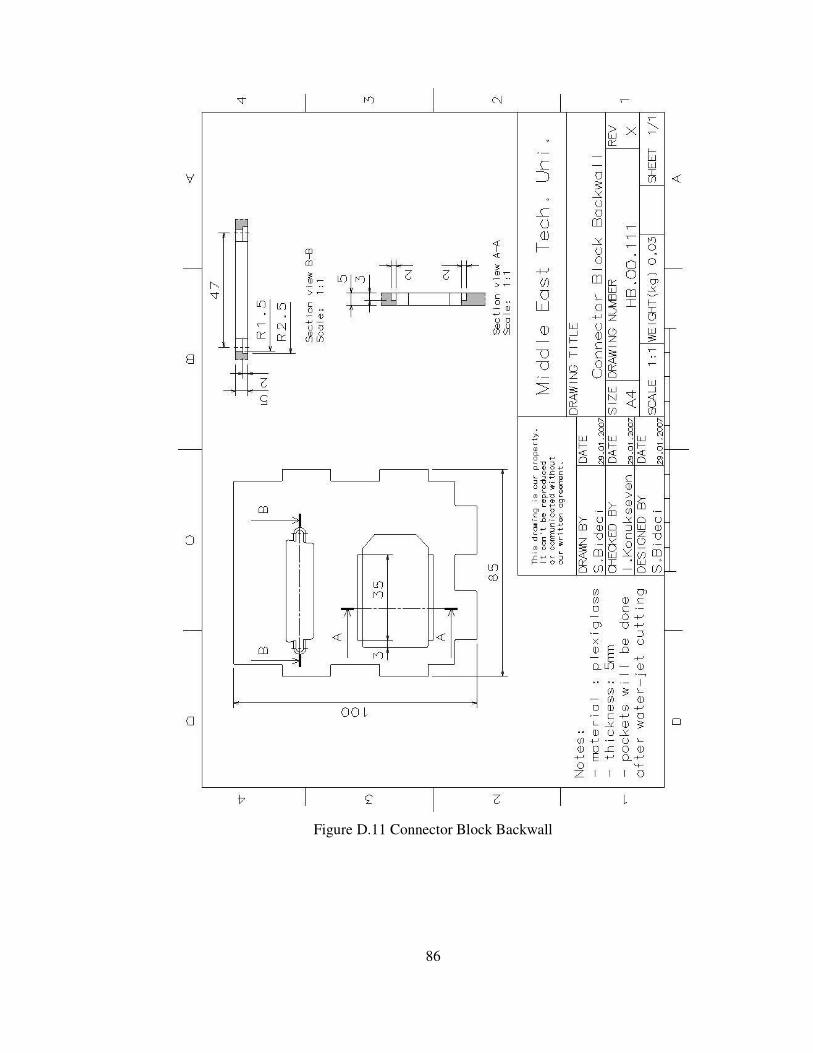
The box is designed using mechanical, electromechanical and electronic components.
The frame is formed by plexiglas parts cut out from sheets. The drawings of the
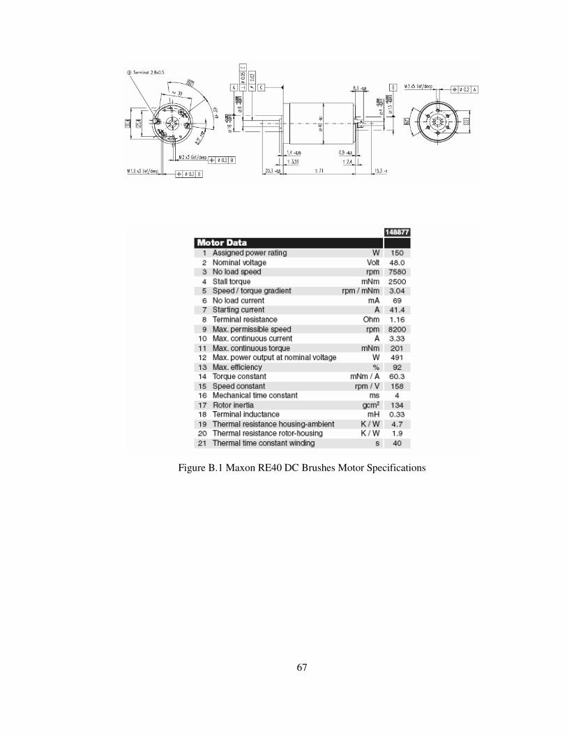
manufactured parts are given in Appendix D. The actuating unit is a MaxonRE40 DC
brush motor which has a 150W power. It is connected to a Copley413CE DC Brush
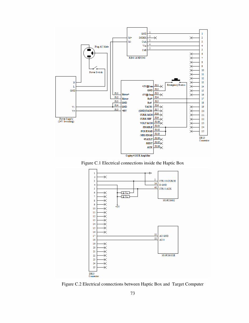
Servo Amplifier. The diagrams for electrical connections of the box are given in
Page 25
12
Appendix C. The motor torque is amplified using sprocket and chain by a 128/18
ratio. User interaction is maintained by the knob attached to the large sprocket, and
the motion is sensed by a HP HEDS5540A optical encoder attached to the rear side
of the motor. Specifications for off-the-shelf components are given in Appendix B.
3.1 Haptic Box Specifications
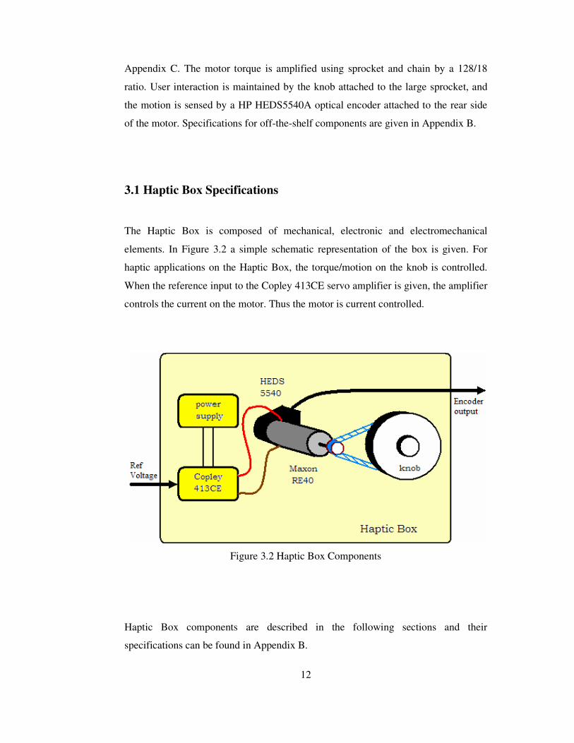
The Haptic Box is composed of mechanical, electronic and electromechanical
elements. In Figure 3.2 a simple schematic representation of the box is given. For
haptic applications on the Haptic Box, the torque/motion on the knob is controlled.
When the reference input to the Copley 413CE servo amplifier is given, the amplifier
controls the current on the motor. Thus the motor is current controlled.
Figure 3.2 Haptic Box Components
Haptic Box components are described in the following sections and their
specifications can be found in Appendix B.
Page 26
13
3.1.1 Copley 413CE DC Brush Servo Amplifier
Copley 413CE is a servo amplifier for DC brush motors. With its torque and velocity
modes, motor torque and velocity can be controlled easily using an analog ±10V
reference voltage. The amplifier is excited with 24V voltage from an external power
supply (requires a minimum of 2.7W). It can supply a peak power of ±30A@±80V
for a peak time of 1 second maximum. Copley 413CE comes with default
adjustments however some important values can be set using the 40-pin socket. As
the Haptic Box is a torque control device, current limitation becomes conceivable.
Using proper resistances on the socket continuous and peak current values and peak
time can be limited.
3.1.2 Maxon RE40 DC Motor and Optical Incremental Encoders
Maxon RE40 is a 150W DC motor with graphite brushes. It has a 48V nominal
voltage, but can be used at lower voltages in this study. The motor can
generate 2500mNm stall torque, and has a torque constant mNmK a 3.60= .
At the back of the motor, there is a HP HEDS 5540A optical encoder attached. The
encoder has 500 lines per revolution for A and B channels and it also has an index
channel. We have also used a Scancon encoder for velocity and acceleration
monitoring. It has 5000 pulse at A and B channels, and an additional index channel I.
3.1.3 Other Components
There are some other components which are necessary for the proper functioning of
the system. Two sprockets and one chain twined on them are first group of them.
They transmit the torque from one to the other. The small sized one is attached to the
shaft of the motor and it has 18 teeth. The large one is attached to the shaft to which
Page 27
14
knob is attached and it has 128 teeth. Thus, a 128/18 gear ration is used to amplify
the motor torque. Another unit to complete the system is the emergency button. As
the Maxon RE40 is a powerful motor, an emergency button is added to the system.
For conformation and some control applications a torque transducer is also used.
Page 28
15
CHAPTER 4
HAPTIC CONTROL
Haptic devices are the manipulators which can be controlled by some ways similar to
robot control methods. However, haptic devices must be taken into account as a
whole system, as haptic interfaces, and the haptic interface control should be done
keeping this fact in mind. Since the haptic interfaces are force reflecting system,
force is the controlled value.
The origin of haptic devices dates back to 1950’s. In these years master arms are
used in radioactive applications. Later on, force sensing capability is added to those
devices that were proportional to the felt force at the slave. With the computational
power of computers, more complex master arms are built. After a period of time,
researchers realized that these devices could have been used in virtual and real
applications for reflecting forces and these Force Reflecting Hand Controllers
belonging to a class of robotic mechanisms usually referred to as haptic devices [22].
Most of the haptic devices in the market does not have force sensing capability
because of the price of the force transducers and the price of the implementation of
these sensors to the system. Therefore, these devices are open loop force controlled.
However, this method requires a lightweight device structure not to effect dynamics
of the application by the device dynamics. When larger workspaces and force
capabilities are required device structure becomes more cumbersome. In this case,
force feedback becomes vital [23].
In this chapter, first general robot control algorithms will be given, than the haptic
control method will be explained. The general structures of the following titles are
Page 29
16
taken from studies of Ueberle and Buss [23]. In order to make it clear thorough the
rest of the chapter, first impedance and admittance terms will be described firstly.
4.1 Impedance & Admittance
Parts forming any system have some dynamic properties. These properties become
apparent when a single part or systems of parts move. Depending on these properties
some forces act on the part bodies that can be grouped as inertial, gravitational,
frictional, coriolis, centrifugal and external forces. The sum of these forces in vector
domain gives the net force that causes the body to move. There is a relationship
between the net force on the body and the body motion. This relationship can be
modeled mathematically by some differential equations. However, those differential
equations are generally complicated and using them in description of system
structures (not in details) becomes incomprehensible. Therefore, more
understandable terms are used for those relations. These relationships are called
impedance and admittance of a body or a system.
In electrical applications the term impedance is used to define the total resistance to
the current flow of a body. This can be used to define impedance for mechanical
systems as the total resistance of a body to motion and this resistance is felt as a
force. Thus, impedance is the relation between the body motion and the total force
acting on it and it is denoted by the capital letter Z . Impedance can be written
mathematically as:
xZf &*= (4.1)
Here f is used to denote both force and torque and it is called generalize force, and
x& is used to represent motion (position, velocity, acceleration) and it is called
generalized motion.
Page 30
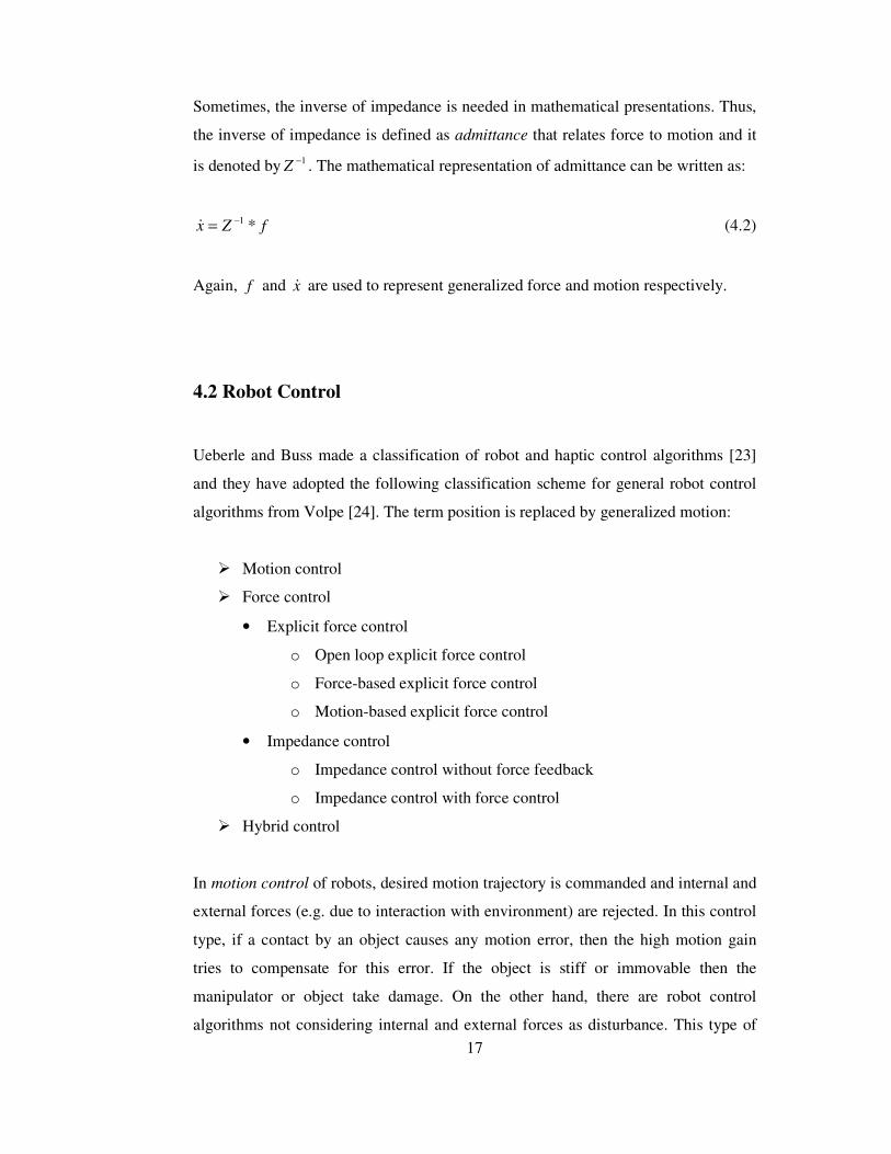
17
Sometimes, the inverse of impedance is needed in mathematical presentations. Thus,
the inverse of impedance is defined as admittance that relates force to motion and it
is denoted by 1−Z . The mathematical representation of admittance can be written as:
fZx *1−=& (4.2)
Again, f and x& are used to represent generalized force and motion respectively.
4.2 Robot Control
Ueberle and Buss made a classification of robot and haptic control algorithms [23]
and they have adopted the following classification scheme for general robot control
algorithms from Volpe [24]. The term position is replaced by generalized motion:
� Motion control
� Force control
• Explicit force control
o Open loop explicit force control
o Force-based explicit force control
o Motion-based explicit force control
• Impedance control
o Impedance control without force feedback
o Impedance control with force control
� Hybrid control
In motion control of robots, desired motion trajectory is commanded and internal and
external forces (e.g. due to interaction with environment) are rejected. In this control
type, if a contact by an object causes any motion error, then the high motion gain
tries to compensate for this error. If the object is stiff or immovable then the
manipulator or object take damage. On the other hand, there are robot control
algorithms not considering internal and external forces as disturbance. This type of
Page 31
18
control is called force control. Force control schemes can be grouped as explicit
force control and impedance control.
In explicit force control algorithms the desired interaction force is commanded.
Explicit force control algorithms with no force feedback are called open loop explicit
force control. Other implementations use the force feedback to compare it with the
commanded force and control error is obtained. This control error is then used to
control the plant directly (force-based explicit force control), or it is first transformed
into a reference motion through an admittance and then it is given to a motion
controller (motion-based force control). This type of control is also known as
admittance control.
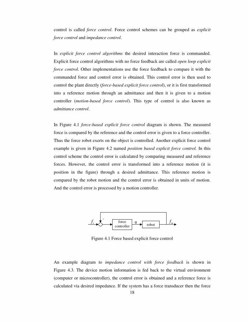
In Figure 4.1 force-based explicit force control diagram is shown. The measured
force is compared by the reference and the control error is given to a force controller.
Thus the force robot exerts on the object is controlled. Another explicit force control
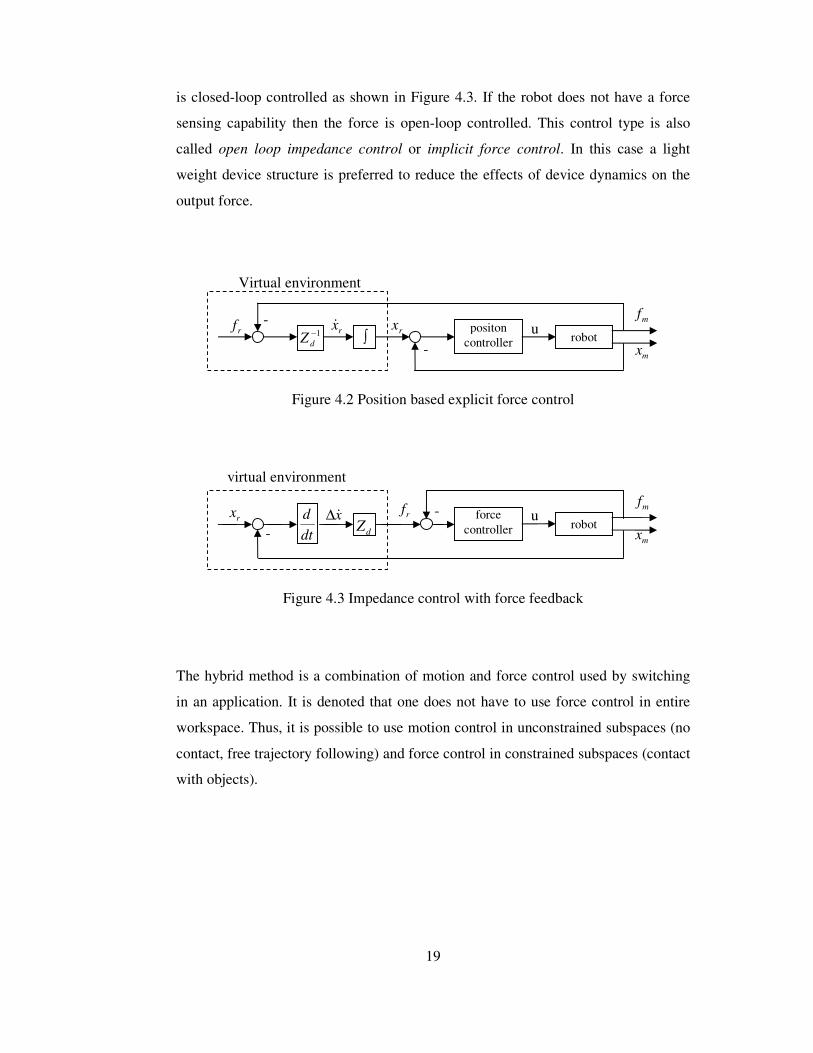
example is given in Figure 4.2 named position based explicit force control. In this
control scheme the control error is calculated by comparing measured and reference
forces. However, the control error is transformed into a reference motion (it is
position in the figure) through a desired admittance. This reference motion is
compared by the robot motion and the control error is obtained in units of motion.
And the control error is processed by a motion controller.
Figure 4.1 Force based explicit force control
An example diagram to impedance control with force feedback is shown in
Figure 4.3. The device motion information is fed back to the virtual environment
(computer or microcontroller), the control error is obtained and a reference force is
calculated via desired impedance. If the system has a force transducer then the force
force controller robot
u rf -
mf
Page 32
19
is closed-loop controlled as shown in Figure 4.3. If the robot does not have a force
sensing capability then the force is open-loop controlled. This control type is also
called open loop impedance control or implicit force control. In this case a light
weight device structure is preferred to reduce the effects of device dynamics on the
output force.
Figure 4.2 Position based explicit force control
Figure 4.3 Impedance control with force feedback
The hybrid method is a combination of motion and force control used by switching
in an application. It is denoted that one does not have to use force control in entire
workspace. Thus, it is possible to use motion control in unconstrained subspaces (no
contact, free trajectory following) and force control in constrained subspaces (contact
with objects).
force controller robot
virtual environment
rf
dZ dt
d
mf
mx -
- rx x&∆ u
positon controller robot ∫
mf
mx
-
-
rx rx& u
Virtual environment
1−
dZ rf
Page 33
20
4.3 Haptic Control
A good description of control strategy of haptic interfaces is made by Ueberle and
Buss as: “The haptic simulation of a human’s bilateral interaction with a virtual or
remote environment requires the control of the motion-force relation between the
operator and the robot.” [13]. A comparison for robot and haptic system controls can
be made as follows: Robot control requires a reference data given by a computer or
microcontroller in means of motion trajectory or force to maintain and the system
tries to follow that reference. However, in haptic interfaces, the motion of haptic user
is assumed to be the reference. Accordingly, a force is reflected to the user and his
/her motion is affected by the system. That is to say, in haptic systems a user and
machine interaction is present.
Most of the simulators built so far are concentrated on modeling virtual
environments and used relatively simple control algorithms [22]. There are two main
class of haptic control schemes used. The first one is impedance display mode and
the second one is admittance display mode. The classification is made according to
the behavior of the virtual environment. As the admittance is conversion of force to
motion, force feedback is required. However, in impedance display force feedback is
not a requirement.
4.3.1 Impedance Control
In impedance control shown in Figure 4.4, the virtual environment acts as impedance.
It accepts motion and produces a respective force. In the figure dZ is the desired
virtual environment impedance, 1−rZ is the robot admittance, EEZ is the impedance
of the end-effector which is between force sensor and the user. The parameter with a
hat symbol shows that it is the model of that parameter.
Page 34
21
Figure 4.4 Impedance control with force feedback and model feed forward
From the block diagram, the following equation can be derived:
[ ] [ ][ ][ ]xZZfxZGxZfJZZIZJx EEEEdcd
T
r
j
r
j
r
j&&&& ˆˆ 111 −++−−−−=
−−− (4.3)
Here cG is the transfer function of the controller. From Eq.4.1 the following
equation for closed-loop impedance relating the device motion x& to the operator
force f− can be obtained arithmetically as:
[ ] [ ][ ]EEEEcrrcdRCL ZZGZGIZZ ˆˆ1−+−++=
− Z (4.4)
RCLZ gives the impedance of the system, that is, it gives the dynamic relation
between device motion to the operator force. It can be shown mathematically as:
xZf RCL&=− (4.5)
The desired haptic system should reflect the virtual/remote environment properties
precisely. Thus the closed-loop impedance RCLZ of the system should represent the
desired virtual environment impedance dZ ( )dRCL ZZ ≅ . This shows that force
dZ−rf
sensor
TJcG
rj Z
∧
1−
r
jZ
fwdτ
inτ•
q•
xJ
TJEEZEEZ
∧
-
f
mτ
τ
sf-
-
Page 35
22
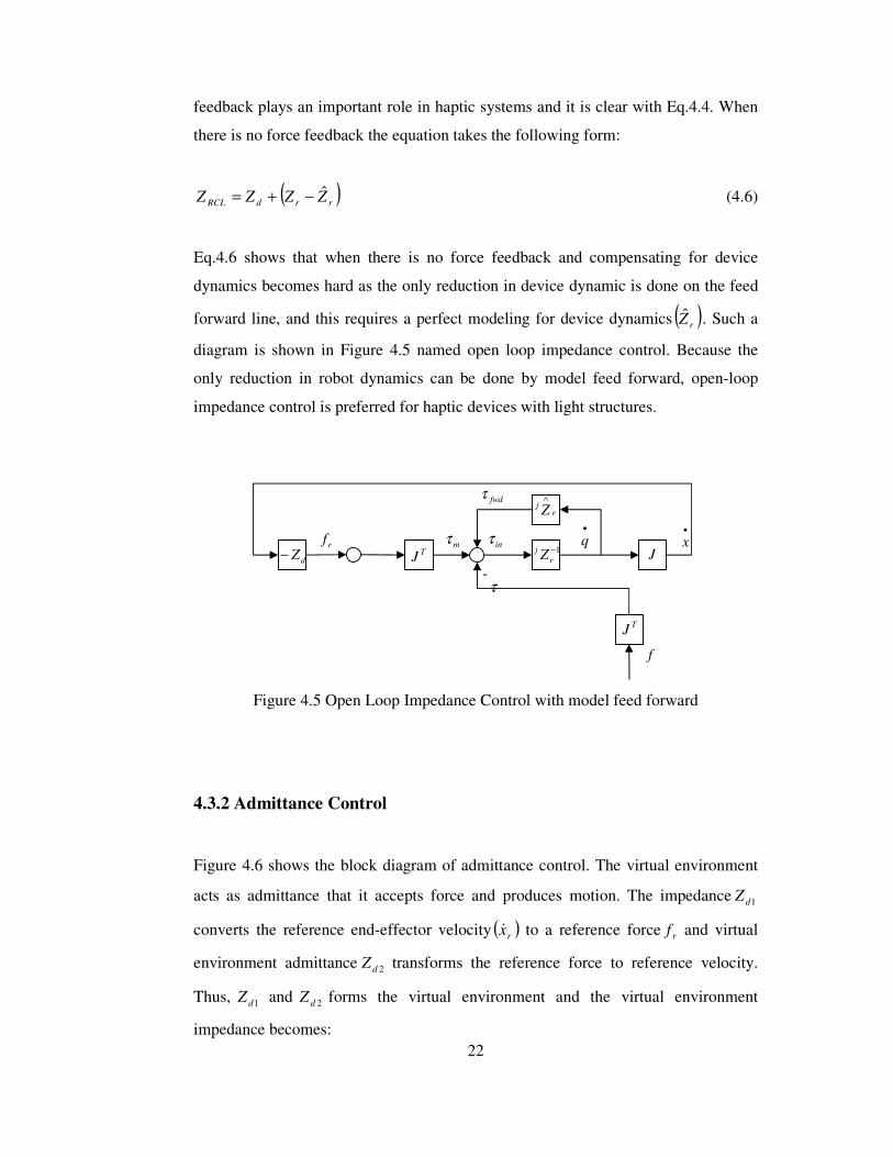
feedback plays an important role in haptic systems and it is clear with Eq.4.4. When
there is no force feedback the equation takes the following form:
( )rrdRCL ZZZZ ˆ−+= (4.6)
Eq.4.6 shows that when there is no force feedback and compensating for device
dynamics becomes hard as the only reduction in device dynamic is done on the feed
forward line, and this requires a perfect modeling for device dynamics ( )rZ . Such a
diagram is shown in Figure 4.5 named open loop impedance control. Because the
only reduction in robot dynamics can be done by model feed forward, open-loop
impedance control is preferred for haptic devices with light structures.
Figure 4.5 Open Loop Impedance Control with model feed forward
4.3.2 Admittance Control
Figure 4.6 shows the block diagram of admittance control. The virtual environment
acts as admittance that it accepts force and produces motion. The impedance 1dZ
converts the reference end-effector velocity ( )rx& to a reference force rf and virtual
environment admittance 2dZ transforms the reference force to reference velocity.
Thus, 1dZ and 2dZ forms the virtual environment and the virtual environment
impedance becomes:
dZ−rf
TJ
rj Z
∧
1−r
j Z
fwdτ
inτ•
q•
xJ
TJ
f
mτ
τ-
Page 36
23
21 ddd ZZZ += (4.7)
If the inner loop position controller gain is sufficiently large then the closed-loop
impedance of the system becomes:
EEEEdRCL ZZZZ ˆ−+≈ (4.8)
End-effector terms takes place in Eq.4.8 as the force transducer is places just before
the end-effector. It is pointed by Ueberle and Buss that by this method providing a
more natural feel to the operator is possible compared to impedance control that does
not apply model based inertia compensation. However, on the other hand, extracting
reference position from force error adds more poles than zeros and this increases the
phase lag in the system’s open-loop transfer function.
Figure 4.6 Admittance Control
1dZ−rf
sensor
1−
r
jZ
inτ q&J
EEZEEZ
∧
-
f
mτ
τ
sf-
1
2
−
dZ ∫
rx& rx position controller
acc controller
cx&&
rx&&
TJ∫ TJ
- -
x&
d__dt
Page 37
24
4.3.3 Haptic Control Conclusions
There are many studies in the haptic field and they are generally on developing some
interfaces for some application such as virtual simulators for art, medical, military,
etc., simulations. These kinds of works generally depend on buying a commercial
haptic device and combining it with a computer to form the haptic interface. As they
are on the shelf products their software and electronics comes within the package and
the user implements the haptic device to his/her interface directly. Thus there is not a
choice for choosing the control law for that device. Generally, haptic devices on the
market do not have any force transducer attached to the gripper and so they are
controlled with open-loop impedance control algorithms. Therefore, the virtual
environment being simulated is tried to be modeled so as the haptic device can
reflect forces in that environment.
On the other hand, some studies compares impedance and admittance display modes
with the same hardware. Ueberle and Buss examined the control methods for haptic
devices and concluded that there is not a best one between these control algorithms
[23]. Carignan and Cleary made a similar study and concluded that one method is not
superior to the other. However, it is pointed that the admittance controller gives
better results at lower impedance values, and the impedance control is superior for
higher impedances values being simulated. [22].
Page 38
25
CHAPTER 5
VELOCITY AND ACCELERATION ESTIMATION
Incremental optical encoders are widely used in many robotic and mechatronics
applications. An incremental optical encoder is basically a disk with very low inertia
and hollow lines on it and some electronic components. As the disk rotates, a photo-
transistor generates a square wave (0-5 Volts) according to the solid-hollow stages of
the disk. A region on the disk with solid and hollow sections is called a channel. The
signal is read from the channel of the encoder, and decoded according to its rising
and falling edges. If the encoder has two channels in quadrature, it can be read in 1X,
2X and 4X decoding modes which increases the resolution 1, 2 and 4 times
respectively.
Velocity and acceleration measurements are required in advanced control
applications to improve the effect of the controllers on the system. On the other hand,
in haptic applications, for a realistic simulation, velocity and acceleration data is
required to reflect the damping and inertial forces of the simulated environment
besides position which is used to simulate the stiffness property. Tachometers and
accelerometers are direct solutions for velocity and acceleration measurement;
however they occupy large spaces, add inertia to the joints, have a noisy output and
they are expensive. Additionally, in recent years, micro processors ( )Psµ and Digital
Signal Processors ( )DSPs are used widely in digital systems. Their widespread
usage also makes it easier to implement encoders to digital systems. Thus, encoders,
which are very precise position measurement devices, are good value for velocity
and acceleration estimations from discrete position data.
Encoders are used for position measurement and they do not measure velocity and
acceleration directly. As an encoder produces a square wave signal, position data can
Page 39
26
not be gathered continuously or at every sample. This signal is a discrete signal and
its frequency depends on its resolution for a constant shaft velocity. Obtaining
precise velocity information from this discrete signal is a challenging work,
especially for low velocities [4]. There are many methods proposed in the literature
to estimate velocity from discrete position and time data. General applications are on
processing position and time data using arithmetic operations at specified sampling
times. This type of applications are easy to implement but have some problems at
some velocity regions. Besides, Kalman filters can also be used to estimate velocity
from incremental encoder output and they give good results. These methods are
described below and to show their performance on the Haptic Box some of them are
tried experimentally.
5.1 Velocity Estimation Methods in Literature
Most of the studies on velocity estimation from an incremental encoder data show
that there is not a way suitable for every velocity profiles [2,6,26]. In [2,26], some
velocity estimators; lines per period (LPP), reciprocal-time, Taylor series expansions,
backward difference expansions, and least square curve fits are presented. It is
pointed in [2] that the least-squares velocity estimators filtered the measurement
noise best, whereas the Taylor series expansions and backward difference equation
estimators respond better to velocity transitions. In [26] it is concluded that using
fixed-time algorithms for high-speed, fixed-displacement algorithms for low-speed,
and least square fit algorithms for general situations proved advantageous. An
adaptive sampling rate is used in [3], in which the sampling rate is changed
adaptively for different velocities. In [4] a similar way is followed to let the
algorithm to estimate the velocity for different velocities better, allowing the user to
select the estimation precision and time delay. The reference [27] proposes an
adaptive scheme designed in conjunction with a linear observer. In [6] a method
called asynchronous sampling method (ASPM) is presented for determining velocity
in systems with low-variable speeds and/or with low-resolution encoders. The
method uses an auxiliary sampling period to estimate the velocity via an observer. It
Page 40
27
is shown in [28] that counting lines for a regular time period become degraded as
sampling rates increase for velocity and acceleration estimations, and a Kalman filter
is proposed. Kalman filters are widely used for filtering or estimating states in
systems. Thus, it can be applied to velocity estimation for the discrete position data
coming from incremental encoders.
In this study disadvantages of fixed time/position algorithms are explained and
shown. For better estimation results adaptive velocity estimation is employed and
results are evaluated. Finally, Kalman filters are used for velocity and acceleration
estimation. Constant velocity and constant acceleration Kalman filter algorithms are
used and both have given very good results. As acceleration estimation for reflecting
inertia and mass properties is required, constant acceleration model of Kalman filter
is used for the rest of the implementation work. Details of used methods are given in
the following sections and applications are explained in Chapter 6.
5.2 Velocity Estimation Algorithms
Once the position and time information is stored for every sampling time, the first
method one will think of is generally discrete differentiation. However, discrete-time
derivative filters known are not satisfactory and as known derivative operators tend
to magnify errors [26]. It is stated in [3] that arithmetic differentiation introduces
significant error and does not give accurate results at low rotational velocities. Thus,
some techniques are proposed in the literature for estimating velocity from discrete
position data. To estimate the velocity from a discrete position signal, there are two
general ways used. The first one is counting the number of encoder pulses in a
specified constant time period, so time is fixed between two successive position
measurements and this is called fixed-time estimator. The second way is measuring
the time duration to travel a fixed distance, which is called fixed-position estimator
[2].
Page 41
28
5.2.1 Fixed-time Velocity Estimation
Obtaining good estimation values at low velocities are important in haptic
applications to reflect small forces to the user. However, this type of velocity
estimation does not give satisfactory results at low velocities. As the time is fixed,
the number of pulses in this time interval will be less at low velocities resulting in
greater errors in the velocity estimation. On the other hand, for high velocities, the
sampling rate can be increased to decrease delay.
The simplest way of estimating velocity is counting lines per period (LPP) [2]. If at a
sampling instance kt , the measured position is kx the velocity can be estimated as
Txkk /ˆ ∆=υ where 1−−=∆ kkk xxx the traveled distance and 1−−= kk ttT the
sampling interval. Some other methods are also reviewed in the reference. They are
Taylor Series Expansion (TSE) Velocity Estimator, Backward Difference Expansion
(BDE) Velocity Estimator and Least Squares Fit (LSF) Velocity Estimator.
In TSE velocity estimator, the velocity kυ at
kt is estimated from the velocity βυ at
time βt by a Taylor Series Expansion around time instance βt :
( ) ( ) ( ) K+−+−+−+=3
3
32
2
2 ˆ
!3
1ˆ
!2
1ˆ
!1
1ˆˆ
β
β
β
β
β
β
β
υυυυυ tt
dt
dtt
dt
dtt
dt
dkkkk (5.1)
As kυ is sad to be the average velocity during sampling period
kt and it occurs at the
middle of that period then Eq.5.1 becomes
j
kjN
j
k
T
j
=∑
= 2ˆ
!
1ˆ )(
0βυυ (5.2)
where N is the order of the derivative.
Page 42
29
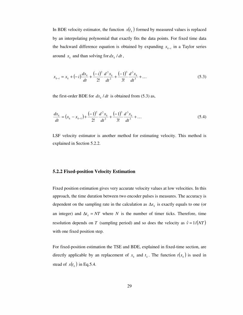
In BDE velocity estimator, the function ( )ktx formed by measured values is replaced
by an interpolating polynomial that exactly fits the data points. For fixed time data
the backward difference equation is obtained by expanding ikx − in a Taylor series
around kx and than solving for dtdxk / ,
( )( ) ( )
K+−
+−
+−+=− 3
33
2
22
!3
1
!2 dt
xd
dt
xdi
dt
dxixx kkk
kik (5.3)
the first-order BDE for dtdxk / is obtained from (5.3) as,
( )( ) ( )
K+−
+−
+−= − 3
33
2
22
1 !3
1
!2
1
dt
xd
dt
xdxx
dt
dx kk
kk
k (5.4)
LSF velocity estimator is another method for estimating velocity. This method is
explained in Section 5.2.2.
5.2.2 Fixed-position Velocity Estimation
Fixed position estimation gives very accurate velocity values at low velocities. In this
approach, the time duration between two encoder pulses is measures. The accuracy is
dependent on the sampling rate in the calculation as kx∆ is exactly equals to one (or
an integer) and NTtk =∆ where N is the number of timer ticks. Therefore, time
resolution depends on T (sampling period) and so does the velocity as ( )NTv /1ˆ =
with one fixed position step.
For fixed-position estimation the TSE and BDE, explained in fixed-time section, are
directly applicable by an replacement of kx and kt . The function ( )kxt is used in
stead of ( )ktx in Eq.5.4.
Page 43
30
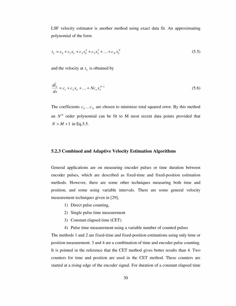
LSF velocity estimator is another method using exact data fit. An approximating
polynomial of the form
N
kNkkkk xcxcxcxcct +++++= K3
32
210 (5.5)
and the velocity at kt is obtained by
121
ˆ−+++= N
knk
k xNcxccdx
tdK (5.6)
The coefficients Ncc K0 are chosen to minimize total squared error. By this method
an thN order polynomial can be fit to M most recent data points provided that
1+> MN in Eq.5.5.
5.2.3 Combined and Adaptive Velocity Estimation Algorithms
General applications are on measuring encoder pulses or time duration between
encoder pulses, which are described as fixed-time and fixed-position estimation
methods. However, there are some other techniques measuring both time and
position, and some using variable intervals. There are some general velocity
measurement techniques given in [29],
1) Direct pulse counting,
2) Single pulse time measurement
3) Constant elapsed time (CET)
4) Pulse time measurement using a variable number of counted pulses
The methods 1 and 2 are fixed-time and fixed-position estimations using only time or
position measurement. 3 and 4 are a combination of time and encoder pulse counting.
It is pointed in the reference that the CET method gives better results than 4. Two
counters for time and position are used in the CET method. These counters are
started at a rising edge of the encoder signal. For duration of a constant elapsed time
Page 44
31
elT waited and at the next rising edge, the encoder pulse after elT , the counters are
stopped. The contents of position counter pC and time counter tC are used to
calculate the average velocity for the periodelT .
A later study using CET method with a variable time step (variable elapsed timeelT )
is proposed in [3]. The method uses the CET technique; however, the desired elapsed
time elT is not fixed. According to the previously estimated velocity data, next
desired sampling interval elT is selected. By this way, an improvement on system
accuracy at low velocities achieved while the response time is decreased at high
velocities.
A simple and efficient method is proposed in [4]. This method allows the user to
select the estimation precision and to tune the time delay, and it requires less
calculation time. It is mentioned that the Euler estimation is the simplest way of
obtaining velocity, if the position is precisely sampled. This is not possible using an
incremental encoder pulse train as it contains stochastic error. An improvement is to
tracking some backward steps, which gives a smoother velocity profile but it
introduces some time delay. R is the encoder resolution and )(tq is the real angular
position of the shaft. If it is sampled with T , the discrete position can be denoted as
)(kθ where ,...2,1=k . Assuming the encoder pulse train is uniform, the position
error can be written as,
Rkqk <− )()(θ (5.7)
When a position segment ))(()( TjkqkTq −− , where ,...2,1=j is selected than the
estimated velocity can be written as,
jvjT
jkkˆ
)()(=
−−θθ (5.8)
If the velocity resolution is defined as T
RvR = than the error in velocity becomes,
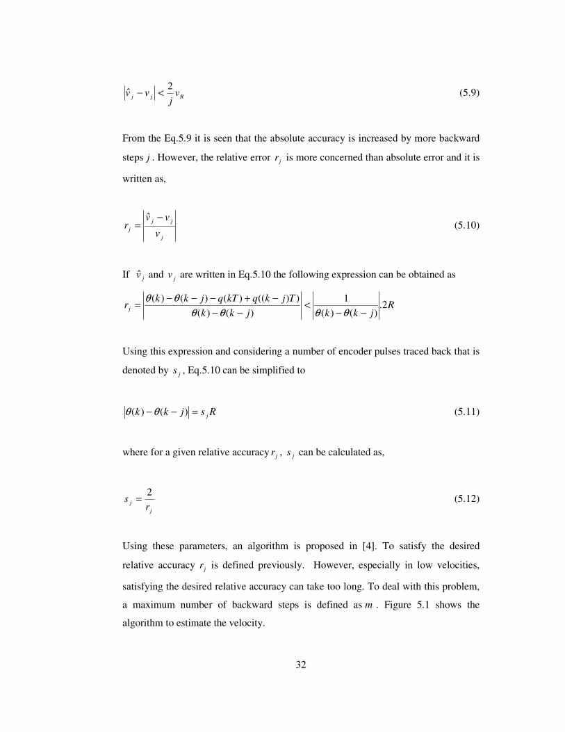
Page 45
32
Rjj vj
vv2
ˆ <− (5.9)
From the Eq.5.9 it is seen that the absolute accuracy is increased by more backward
steps j . However, the relative error jr is more concerned than absolute error and it is
written as,
j
jj
jv
vvr
−=
ˆ (5.10)
If jv and jv are written in Eq.5.10 the following expression can be obtained as
Rjkkjkk
TjkqkTqjkkr j 2.
)()(
1
)()(
))(()()()(
−−<
−−
−+−−−=
θθθθ
θθ
Using this expression and considering a number of encoder pulses traced back that is
denoted by js , Eq.5.10 can be simplified to
Rsjkk j=−− )()( θθ (5.11)
where for a given relative accuracy jr , js can be calculated as,
j
jr
s2
= (5.12)
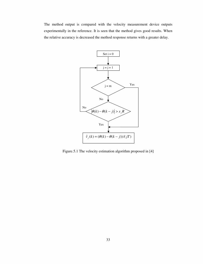
Using these parameters, an algorithm is proposed in [4]. To satisfy the desired
relative accuracy jr is defined previously. However, especially in low velocities,
satisfying the desired relative accuracy can take too long. To deal with this problem,
a maximum number of backward steps is defined as m . Figure 5.1 shows the
algorithm to estimate the velocity.
Page 46
33
The method output is compared with the velocity measurement device outputs
experimentally in the reference. It is seen that the method gives good results. When
the relative accuracy is decreased the method response returns with a greater delay.
Figure.5.1 The velocity estimation algorithm proposed in [4]
Set j = 0
j = j + 1
j = m
)/())()(()(ˆ jTjkkkv j −−= θθ
Rsjkk j>−− )()( θθ
Yes
Yes
No
No
Page 47
34
5.2.4 Velocity and Acceleration Estimation with Kalman Filters
Kalman filters are widely used to filter or estimate states of dynamic systems from
measurements contaminated by random noise. A Kalman filter is an algorithm
proposed by Rudolf E. Kalman in 1960 [7]. It can be applied to the systems with
zero-mean white Gaussian noises [11]. The algorithm predicts the value of a state
according to system parameters and the input to the system and it corrects that value
according to measurement. Thus, it is a prediction/correction algorithm for states of
dynamic systems.
The methods described up to here are about processing position and time data by
arithmetic operations to get the velocity information. At high speeds many of these
methods may work well, but they can not measure velocity correctly at low speeds.
There are also some model based estimators, in which the model parameters and
disturbances must be know accurately and this is not possible for most cases.
Therefore, some models called constant velocity and constant acceleration models
can be employed in Kalman filters, which do not require system information. These
methods, which use kinematic models, are also called kinematic Kalman filters (KKF)
in some references [11]. Kalman filters also provide important advantage to the
stability of the control systems. In the methods requiring a period of time to estimate
the velocity, there is not any information about velocity given to the controller or the
previous velocity is held. However, Kalman filters can provide an estimate of
velocity at every sample time.
By the widespread use of microcontrollers and computers, discrete time
implementations of algorithms became popular and Kalman filters are one of them.
Simply a Kalman filter estimates a value of a state according to previous value and
recent measurement of that state. To do that, the algorithm uses a gain K called
Kalman gain. The simplest form of a Kalman filter with constant K can be given as
[8]:
( ) 11 ˆ1ˆ++ +−= iii KyxKx (5.13)
Page 48
35
Supposing that ix is the best estimate of the state at time i , the state at time ( )1+i
can be estimated from the previous valueix and the recent measurement 1+iy using a
weight between them by the constant K . Here, K determines how much the
measurement is reliable. If measurement is fully reliable than K goes to one ( 1→K ),
and if it is fully faulty than K goes to zero ( 0→K ).
To get familiar with Kalman filter notifications, some matrix presentations are
explained below. G. C. Dean [8] uses i , and )1( +i in the subscript of matrices to
show prediction/correction and time instances. For a constant velocity model of a
system the matrices can be written as:
iix
xT
x
x
=
+ˆˆ
10
1ˆˆ
1&&
(5.14)
whereT is sampling period. In a general form Eq.5.14 can be written as
iiiii XX //1ˆˆ φ=+ (5.15)
X is the state vector defining the system and φ is the state transition vector. Some
of the states are measured in the system to control it. The measurement values are
shown by
1+
iy
y
& (5.16)
and it is represented by 1+iY . Similar to the system defined by a single state in
Eq.5.13, a weighted mean can be written as
1/11/1ˆ)(ˆ
++++ +−= iiiii KYXKIX (5.17)
Page 49
36
where I is the identity matrix and K is 2x2 matrix. The term )/1( ii + in the subscript
in Eq.5.15 show time instance/prediction and the term )1/1( ++ ii in the subscript in
Eq.5.17 shows time instance/correction. Eq.5.13 and Eq.5.17 form the filter to
estimate states with constant Kalman gain K . However, for general applications K is
not constant. In Kalman filtering, system and measurement noises are taken into
account. The system noise is denoted by the capital letter Q . The capital letters P
and R used to represent variances of estimate and measurement noises respectively.
The variance of the new estimate is given by
( )( )[ ]2
111 ˆˆˆ+++ −= iii xExEP (5.18)
( )1ˆ+ixE is the expected value of the new estimate 1ˆ
+ix , Eq.5.18 is the formula for
variance. As is known, the Kalman gain K is tried to be found (for example in
Eq.5.17). And now, it can be calculated by
( ) 1
11/111/11/1ˆˆ −
++++++++ += i
T
iiii
T
iiiii RHPHxHPK (5.19)
where, H is the matrix identifying the measured states. To find K , iiP /1ˆ
+ should be
calculated first.
i
T
iiiiii QPP +=+ φφ //1ˆˆ (5.20)
where,Q is the system noise matrix, and it estimates the modeling errors. Here, the
subscript ( )ii /1+ of iiP /1ˆ
+ means that the matrix P is calculated at time ( )1+i and it
is the predicted one pointed by ( )i . Thus, a correction of it should be calculated as
( ) iiiiii PHKIP /1111/1ˆˆ
+++++ −= (5.21)
to be used in the next calculation time ( )2+i . Thus, all the Kalman equations are
obtained to estimate the states. The Kalman loop can be explained by a diagram as
Page 50
37
shown in Figure 5.2 [10]. For compatibility with the previous notation subscripts are
left as they were but superscripts are changed as it is simpler to understand using the
(-) symbol in the superscript to denote the prediction.
Figure 5.2 Recursive Prediction-Correction Structure of the Kalman Filter
1) Predict the next state
iii uxx ψφ +=−
+ˆˆ
1
2) Estimate the prediction
error
i
T
iii QPiP +=−+ φφ ˆ
1
1) Compute Kalman gain
( ) 1
1111111ˆˆ −
++−+++
−++ += i
T
iii
T
iii RHPHHPK
2) Correct the predicted state using
measurement
( )−
++++
−
++ −+= 111111 ˆˆˆiiiiii xHyKxx
3) Estimate the estimation error
( ) −++++ −= 1111
ˆˆiiii PHKIP
PREDICTION CORRECTION
Initial estimates of ix and iP
Page 51
38
CHAPTER 6
SYSTEM IMPLEMENTATION
The system implementation of velocity estimation and haptic control methods are
given in this chapter. First, the velocity and acceleration estimation from the
incremental encoder is implemented and the results are presented. Next, using the
velocity and acceleration estimation virtual environment characteristics in the system
haptic control is developed. Finally, employing the Virtual Reality Toolbox® of
MATLAB® in the interface the system demonstration is done.
6.1 Experiment Setup
The experimental setup consists of the Haptic Box, target computer and the host
computer as shown in Figure 6.1. The Haptic Box is used as an input and output
device for the user interaction with the system. The target computer is the control
unit of the system. It receives the encoder and transducer signals from the user,
processes them to extract motion and torque information, and trough the control law
it generates a reference voltage to be sent to the servo amplifier of the Haptic Box.
The input-output operations to the target computer are done via the data acquisition
(DAQ) cards. There are two main roles of the host computer. The first is to compile,
download and manage the applications that will run on the target computer via the
LAN connection. And the second is to collect the motion data processed by the target
computer and use it to manipulate the virtual environment on the screen. The
applications running on the target computer are modeled using the Simulink® and
the xPC Target® libraries. Virtual environments are modeled using the VRML
Page 52
39
language and they are simulated using the Virtual Reality Toolbox® of MATLAB®
on the host pc.
Figure 6.1 Haptic Interface
The Haptic Box is explained in Chapter 3. It has a DC Maxon RE40 DC motor and a
HEDS5540A encoder attached to the back of it. The position is read from this optical
incremental encoder discretely. The encoder has 500 lines at A, B channels and it
also has an Index channel. The position is read in 4X counting mode so that the
resolution increases to 2000 counts/rev on the motor side. There is a gear ratio of
18/128 between the motor and the knob of the box. Thus the resolution at the knob
side is (128/18)*2000 counts/rev. There is an encoder with 5000 pulse/rev at A and
B channels. This encoder is attached to the front side of the motor and it is used for
velocity and acceleration monitoring. A torque transducer is also introduced in to the
box that is capable of measuring 10Nm torque load.
Page 53
40
The target computer has a Pentium 1.80 GHz processor and 512 MB of RAM. There
are two DAQ cards to collect data from the system. National Instruments Company
NI PCI-6602 and NI PCI-6052E DAQ cards are used for encoder input and analog
I/O respectively.
The host computer is a HP XW8200 workstation with a Xeon 3.60 GHz processor,
3GB of ram and a NVIDIA Quadro FX 4500 512MB ram graphics card. This
powerful computer is needed for making the real time applications more realistic as a
refresh rate of 30Hz is required for a good perception for human eye and the
simulation sapling period is set to sT 001.0= as the refresh rate for force should be
at last 1kHz [22].
6.2 Velocity and Acceleration Estimations
Velocity estimation methods are described in Chapter5. The first and simplest way is
numerical differentiation, a fixed time method, in which the number of counts in a
period of fixed time is divided by the time period. This method is simple and gives
good results at high speeds. However, when the angular speed is low or the encoder
resolution is decreased the method becomes degraded. As an encoder converts the
motion into a discrete signal, discretization error increases and so the error in
velocity increases as shown in Figure 6.2, at low speeds. Another problem is that if
the period of the encoder output becomes larger than the sampling period than the
same level of the encoder signal (a high level for example) is sampled two times or
more and they get the same value as the position does not change in that time interval.
This results in a zero velocity due to constant position and this situation will be a
problem for stability. To avoid this problem constant position method can be
employed. This method will prevent system from detecting an unwanted zero
velocity but introduce a considerable time delay in to the system. Thus, to avoid
these problems improvements of those methods are developed in the literature.
Constant Elapsed Time (Figure 6.3) can be treated as an improvement to the fixed-
time velocity estimation algorithms, which reduces the discretization errors. In this
Page 54
41
method a constant elapsed time is selected and for this period the system waits.
When this time is reached the next position pulse is waited and time is measured at
this encoder pulse. By this way more accurate velocity estimation is done than a
fixed-time velocity estimation (estimating velocity at elapsed time).
Figure 6.2 Effect of discretization on velocity estimation in low velocity region
Figure 6.3 CET Method
Discretization
error
Page 55
42
6.2.1 Adaptive Velocity Estimation
Another way of improving velocity estimation is using a variable time step. Looking
at the poison data an adaptive algorithm can decide when to calculate the velocity
estimation. In Chapter 5 an adaptive algorithm is presented in Figure 5.1. This
method is implemented using the Haptic Box, and the results are compared to the
monitor velocity, which is obtained from the Scancon encoder that has 5000
pulse/turn at A nad B channels, in Figure 6.4. The algorithm parameters are set as:
sampling time sT 001.0= , number of counts per turn 2000=N , relative accuracy
%5=jr and the time limit for velocity detection 05.0=m (50 ms).
Figure 6.4 Velocity estimation with adaptive algorithm
Figure 6.4 shows that the algorithm works better at higher speeds. In low speed
regions (~230 - 800 ms) the algorithm is forced to calculate a velocity value as the
Page 56
43
maximum allowable time limit is reached. With a relative accuracy %2=jr , as the
accuracy increases more steps back are required, and so more delays are introduced.
6.2.2 Velocity Estimation with Kalman Filters
It is pointed in Chapter 5 that Kalman Filtering is a good estimation method from
noisy data. In this study, a Kalman Filter with Constant Velocity model is used to
estimate velocity and the system is assumed to have zero-mean white Gaussian
noises. In this method the system matrix is a 2x2 matrix as
=
10
1 Tφ (6.1)
and according to Eq.5.15 and Eq.6.1 predicted state values for position and velocity
become
iii xTxx ˆˆˆ 1 &+=−+ (6.2)
ii xx ˆˆ1 && =−
+ (6.3)
After prediction of P matrix as in Eq.5.20, Kalman gain matrix K is obtained as in
Eq.5.19 and correction of predicted states is done as in Eq.5.17 such that
( )−
+++
−
++ −+= 11111 ˆˆˆiiiii xyKxx (6.4)
( )−+++
−++ −+= 11111
ˆˆˆiiiii xyKxx &&&& (6.5)
assuming that the velocity is measured. If velocity is not measured than the
measurement matrix H will have a zero at the right-bottom corner and this will
cancel the effect of Kalman gain and the estimated value will be equal to the
predicted (previous) value in Eq.6.5.
Page 57
44
A Kalman Filter with constant velocity estimation is modeled in Simulink® and it is
run on the target pc in real time. The Kalman algorithm code is embedded into
Simulink® model (Appendix A). Figure 6.5 shows the experiment results. In the
experiment the matricesQ and R are selected as
=
1.00
01.0Q
=
1.00
001.0R
Figure 6.5 Velocity Estimation with Kalman Filter – Constant Velocity model
Q is the system noise matrix and R is matrix that represents the measurement
variances. These matrices are obtained experimentally. It is seen in the experiments
that the changes in system noise matrix Q does not effect the estimation too much
but measurement variance matrix R does a lot. When small values are selected for
11r and 22r then the filter responds fast but some oscillations begin to appear and
Page 58
45
when they are selected larger the filter follows the monitor velocity by some shift
proportional to greatness of the R matrix elements but with a smoother profile. Thus,
an optimum pair for matrix R is tired to be selected. One can recognize that 22r is
greater than 11r . The reason of this is that the encoder gives good position
measurement. However, velocity measurement is obtained by numerical
differentiation and it has greater error. The figure shows that with the selected
parameters the filter gives good results at it is seen in the magnified segment that the
filter has an acceptable time delay (~4 ms).
Actually, most of the haptic applications do not use inertial forces in applications.
Most generally, users touch some surfaces having stiffness and damping
characteristics. However, in this study inertial forces are also aimed and thus
acceleration measurement or estimation is required. For this purpose, general
approach is to use a numerical differentiation after a good velocity profile is obtained.
In the methods that use the numerical differentiation to estimate velocity, the second
differentiation increases the errors more and generally acceleration estimation
becomes impossible. Thus, using Kalman Filters for acceleration estimation becomes
more suitable. To estimate acceleration a constant acceleration model is used similar
to constant velocity model. The state transition matrix for this approach is
=
100
10
2/1 2
T
TT
φ (6.6)
in this case the predicted states can be written as
( ) iiii xTxTxx ˆ2/ˆˆˆ 21 &&& ++=−
+ (6.7)
iii xTxx ˆˆˆ1 &&&& +=−
+ (6.8)
ii xx ˆˆ1 &&&& =−
+ (6.9)
and the corrections are made after prediction of P and calculation of K as in Eq.6.4
and Eq.6.5 for position and velocity, and for acceleration it is made as
Page 59
46
( )−+++
−++ −+= 11111
ˆˆˆiiiii xyKxx &&&&&&&& (6.10)
The code is similar to the one for constant velocity model as given in Appendix A
but with some differences. The matrix φ given in Eq.6.6 and H , P , Q and R
matrices become a 3x3 square matrix and measurement and state matricesY and
X become 3x1 matrices and state order rises to 3.
In the experiment the acceleration measurement is also given to the filter obtained by
the second derivative of the velocity numerically. However, 20 steps back is traced to
make it smoother.Q and R matrices are selected as
=
1.000
01.00
001.0
Q
=
100
01.00
0001.0
R
Figure 6.6 Velocity Est. – Kalman Filter Const. Acc. – Low Velocity Region
Page 60
47
The velocity estimation with inclusion of acceleration measurement can be seen in
Figure 6.6 and Figure 6.7. For both low and high velocity regions the Kalman Filter
gives close results to the monitor velocity and it is clear that it is superior to the
discrete derivation estimator. With current matrix estimations for Q and R the filter
seems to perform well. The filter has a negligible lag (~2ms for low & high velocity
regions) compared to monitor signal.
Acceleration estimation is a more complex work. Using the just previous velocity
measurement data for differentiation increases the errors resulting in increased
oscillations. Thus some steps back are traced to have a smoother acceleration profile.
This profile is used as the measurement data given to the Kalman filter. The result is
compared to the acceleration monitor signal (from Scancon encoder) in Figure 6.8.
The filter gives good estimation results with a little greater delay (~5 ms) than the
one for velocity estimation.
Figure 6.7 Velocity Est. – Kalman Filter Const. Acc. – High Velocity Region
Page 61
48
Figure 6.8 Acceleration estimation with Kalman Filter – Constant Acc. Model
6.3 Control System Applications
In this section velocity/acceleration estimation and haptic control implementations
are presented. The applications demonstrate the control algorithms mentioned in
Chapter 4, Virtual Reality for visual perception and effects of estimations of velocity
and acceleration on the force feeling.
For output confirmation and different control applications, a force transducer is
attached to the back side of the knob of the Haptic Box. The relation between output
voltage and the input torque is not given in the specifications of the transducer and it
is found experimentally as show in Figure 6.9. A torque arm is fixed to the front side
of the transducer and from a 10cm distance several weights are applied. The relation
between torque and voltage is shown in the figure. For getting a constant tK
converting the output voltage to the corresponding torque value, a line is fit to the
Page 62
49
max & min values of the measurements as seen in the figure and its slope is
calculated. This assumption is done depending on the linear transition seen in the
figure. The voltage-torque constant is calculated as
]/[027.1 VNmK t =
Figure 6.9 Transducer output voltage & torque input relation
Another component that has to be experimented for obtaining a constant parameter
was the Copley 413CE servo amplifier. It is configured to torque mode so for a given
voltage it applies a corresponding current to the DC brush motor. However the
relation between reference voltage and current output was not known. Thus, firstly
the motor is replaced by a 5W 33R resistor and current flowing through it measured
for different voltages. Second, the motor is replaced by the resistor and its shaft is
held stationary. It is seen in the experiments that the relation was linear as shown in
Page 63
50
Figure 6.10 (test results with motor). A line is fit to the max & min values and the
slope of the curve, that is the constantavK is calculated as
]/[6385.0 VAK av −=
Figure 6.10 Copley 413CE reference voltage & output current relation
After the constants tK and avK are obtained, a variable reference voltage is given to
the amplifier and the corresponding torque is compared by the measured one. It was
seen the profiles show the same characteristics but reference torque leads measured
torque in both negative and positive torque values in means of torque magnitude.
This showed that the calculated measurement constant tK was greater than it had to
be. This comment is done depending on the fact that the test for Copley 413CE was
much more reliable than the test for transducer calibration. The measurement
constant is lowered to
Page 64
51
]/[0.1 VNmK t =
and the two curves were nearly coincided as shown in Figure 6.11. The aim of the
following experiments are not measuring true values of applied forces but measuring
the effectiveness of the interface. Fast transitions at high torque values cause an
amount of delay (~20ms) or error because of the inertia added to the system by the
transducer and its attachments. The transducer gives a noisy voltage output at
transitions and it has to be filtered. Thus, a Kalman filter is also used here to
smoothen the transducer output as shown in the figure with the red color. The code is
similar to the one given in Appendix A and parameters were set as
0005.0=Q , 1.=R , 1=H
Figure 6.11 Reference, measured and estimated torques
Page 65
52
6.4.1 Open Loop Impedance Control
As the reflection of the reference force to the user is confirmed, control algorithms
can be experimented. Open loop impedance control is the most generally used and
simple control scheme. Beginning with it makes it easier to understand other
methods. In this control type, simply the motion of the Haptic Box knob is acquired
and through the virtual environment a reference force is calculated to be reflected to
the user. For this experiment a virtual disk is modeled that has inertia and it was
connected to the ground by a spring and a damper pair. The Simulink® model of the
interface is showed in Figure 6.12 and block details are given in Appendix E.
Figure 6.12 Simulink model of open loop impedance control
As stated before in these experiments the effects of Kalman Filter is also important
and it is also mentioned. In the experiments with open-loop impedance control it was
seen that after certain inertia and damping force limits, the system became unstable.
Actually, when the parameters for inertia and damping set high and than the
simulation started the knob starts to oscillate. At low speeds velocity estimation error
is much higher. When the knob is stationary at initial position velocity and
acceleration are zero and no corresponding torque is applied to the knob. However,
when the user just touches to the knob a small motion with larger error compared to
high speed error occurs. This error magnifies by inertia and damping gains. This
starts an oscillation and system behavior becomes unstable. Thus, several
experiments are done to determine those parameters. The transducer is detached from
the Haptic Box to reduce unmodeled dynamics that affects inertia gain limit too
much. Sampling period is set to sT 001.0= for the experiments. The power supply
Page 66
53
characteristics are not certain. However it is determined that a torque value of Nm3±
on the knob can be generated by the motor.
The Virtual Environment is a model with stiffness, damping and inertia and the
reference force is calculated as
θθθτ ˆˆˆkbIref ++= &&& (6.11)
Where θθθ ˆ,ˆ,ˆ &&& are estimated angular acceleration, velocity and position values
coming from the Kalman Filter. They are multiplied by the corresponding constants
and added to each other to calculate the reference torque. In the experiments it is
seen that the stiffness gain k does not have a limit value affecting stabilization. Also,
it is seen that oscillations begin at about ]/*[5.1 radsNmb = damping coefficient
and ]/2^*[0045.0 radsNmi = inertia. This value corresponds to the inertia of an
aluminum disk with cm1 thickness and cm3.20 diameter.
6.4.2 Impedance Control with Force-feedback
Impedance control with force feed-back is done employing the torque transducer
actively in the interface as shown in the Figure 6.13. The measured torque is
compared by the reference torque and torque error is given to the force control block
as an input. A proportional control law is used to control the force.
For reference torque calculation Eq.6.11 is used again. The output of the filter gives a
very smooth voltage output. P control law is used in the force control block and it
was set as 2.0−=pK . By this method the maximum damping coefficient that can be
reflected satisfying stability was ]/*[2 radsNmb = and the inertia was
]/2^*[005.0 radsNmi = . This value corresponds to the inertia of an aluminum disk
with cm1 thickness and cm84.20 diameter.
Page 67
54
Figure 6.13 Impedance control with force-feed back
6.4.3 Admittance Control
Figure 6.14 Admittance Control
In admittance control the force is supplied to the virtual environment and motion is
taken out through the desired admittance as shown in Figure 6.14. The reference
motion is calculated using the Eq.6.11. As in the admittance display mode the input
is force and the output is motion the equation must be reversed. Thus, Laplace
transform of the equation was taken assuming zero initial conditions and Eq.6.12 is
obtained.
)(1
)(2
skbsIs
s τθ++
= (6.12)
Once the measured torque is given to Eq.6.12 the knob position is obtained. After
that a position controller can be employed to control device position. In the
Page 68
55
experiments with admittance control a spring model as a virtual environment was
simulated and it was seen that the interface works well. However, the experiments
for damping and inertia reflection did not perform well as the system was unstable.
6.4 Case Study
In haptic interfaces the control loop is closed by the virtual environment. The virtual
environment in the haptic interface is the place where the reference control input is
generated. The reference input is calculated according to the virtual environment
properties, and it is given to the control unit in the form of force or motion according
to the type of the display mode as described in Chapter 4.
For representing virtual environments, different methods can be used. A 3D
environment for representing the virtual environment would be the best way to make
it realistic. Thus, several 3D modeling languages are used in such applications.
OpenGL® and DirectX® are most popular platforms for developing those
environments and VRML (Virtual Reality Modeling Language) is another language
to model interactive virtual environments. As the general application platform for
system implementation is decided to be MATLAB® and Simulink®, the preferred
language for developing virtual environments is VRML, as Simulink® uses this
language to simulate virtual models in its Virtual Reality Toolbox®.
The virtual environment of the haptic interface is modeled so that it contains mass,
damper and spring. The Virtual Reality Toolbox® of Simulink® is used to display
and simulate the virtual environment. Virtual Reality Toolbox® accepts the virtual
environments modeled using VRML language. Thus, the environment is modeled
using a CAD program and it is saved as a VRML file. There is a program coming
with MATLAB® named vrbuil2 which can also be used to model the virtual
environments. In this study it is used to modify the VRML file created by the CAD
program previously. After modeling of virtual environment is complete, Virtual
Reality Toolbox® is used to add it to the interface. Blocks of this toolbox can access
Page 69
56
the objects in the modeled virtual environment. Their position, orientation, scale, etc.,
can be modified in real-time according to the rules defined by the Simulink® model.
This is the method used in this study to visualize the virtual environments as shown
in Figure 6.15.
Figure 6.15 Simulated Virtual Environment
As the Haptic Box is a 1DOF haptic device the virtual environment is also modeled
as a 1DOF mechanism as shown in Figure 6.15. The knob with blue-white color is
the part the user interacts with via the Haptic Box knob. As the user rotates the knob
the knob motion is converted to a linear motion, by a rack and pinion mechanism,
which is identical with the motion of the mass which is yellow colored. To the left
side of the mass a spring and damper couple is attached to apply stiffness and
damping effects to the mass and so the user. The virtual knob does not have dynamic
Page 70
57
properties so it does not add inertial forces to the system. The open loop impedance
control algorithm is used to control the interface.
Page 71
58
CHAPTER 7
CONCLUSION
7.1 Conclusions
In this study Haptic Devices are presented and their control strategies are explained.
In the way trough the control applications importance of precise motion
measurement/estimation is emphasized. General velocity estimation algorithms are
examined and Kalman Filters is found to be the best. As stated in the related chapter
acceleration estimation from an incremental encoder is not examined too much in the
literature. And, acceleration estimation using the Kalman Filter is made and found to
perform well. Control strategies are tried experimentally by employing the motion
estimators modeled previously. It is gathered from the experiments that the feeling of
touch is not affected by the motion estimator, that is to say the estimator does not
unstabilize the system.
The control schemes are experimented and satisfactory results are taken from the
interface. Especially inertia feeling with open loop impedance and impedance control
with force feed-back algorithms were very good. Stiffness and damping feeling was
very sensible. The inclusion of force feed-back into the control strategy increases the
capability of the interface as the maximum values for inertia and damping were
increased.
Tests for admittance control algorithm was also done and unsatisfactory results are
taken from the system. The reason was depending on the modeling errors. From
these results it can not be concluded that admittance control strategy is not a suitable
algorithm.
Page 72
59
7.2 Future Work
The interface works well but admittance control algorithm can be studied more and
implementation with this algorithm can be done. The Haptic Box is a 1 DOF haptic
device and can only simulate 1 DOF virtual/remote environments. For more
flexibility a new haptic device with more freedoms can be constructed. As the
degrees of freedom increases the control strategy becomes more complicated. For
this new device new control strategies can be experimented and new algorithms can
be developed.
Page 73
60
REFERENCES
[1] Marc Ueberle, Martin Buss, “Design, Control, and Evaluation of a new 6DOF
Haptic Device”, Proceedings of the 2002 IEEE/RSJ Intl. Conference on Intelligent
Robots and Systems, pp. 2949-2954, EPFL, Lausanne, Switzerland, October 2002.
[2] Ronald H.Brown, Susan C.Schneider, and Michael G.Mulligan, “Analysis of
Algorithms for Velocity Estimation from Discrete Position versus Time Data”, IEEE
Transactions in Industrial Electronics, Vol.39, No.1, February 1992
[3] J.N. Lygouras, “Accurate Velocity Evaluation Using Adaptive Sampling
Intervals”, Microprocessors and Microsystems 24, 2000, pp. 269-275
[4] G. Liu, “On Velocity Estimation Using Position Measurements”, Proceedings of
the American Control Conference, Anchoage, AK May 8-10, 2002, pp. 1115-1120
[5] Robert D. Lorenz, Keith Van Patten, “High resolution velocity estimation for all
digital, AC servo drives”, IEEE, 1988.
[6] Se-Han Lee, Ty A.Lasky, and Steven A.Velinsky, “Improved Velocity
Estimation for Low-Speed and Transient Regimes Using Low-Resolution Encodes”,
IEEE,ASME Transactions on Mechatronics, Vol.9, No.3, September 2004
[7] R.E. Kalman, “ A new approach to linear filtering and prediction problems”,
Transactions of the ASME-Journal of Basic Engineering, 82(Series D):35-45, 1960
[8] G.C. Dean, “An introduction to Kalman filters”, Measurement + Control, Volume
19, March 1986, pp:69-73
[9] Heui-Wook Kim, Seung-Ki, “A new motor speed estimator using Kalman filter
in low-speed range”, IEEE Transactions on Industrial Electronics, Vol. 43, No 4,
August 1996
Page 74
61
[10] Ge Yang, “A practical introduction to Kalman filtering”, Technology and
Algorithms Seminar, Department of Cell Biology, TSRI, July 22, 2004
[11] Soo Jeon, Masayoshi Tomizuka, “Benefits of acceleration measurement in
velocity estimation and motion control”, Control Engineering Practice 15, 2007,
pp:325-332
[12] Jesse D. Hwang, Michael D. Williams, Günter Niemeyer, “Toward Event-Based
Haptics: Rendering Contact Using Open-Loop Force Pulses”, Proceedings of the 12th
International Symposium on Haptic Interfaces for Virtual Environment and
Teleoperator Systems, HAPTICS’04.
[13] SensAble Technologies, Phantom Haptic Devices,
http://www.sensable.com/haptic-phantom-premium-6dof.htm, last access July 2007.
[14] Immersion Corporation, CyberGraspExoskeleton,
http://www.immersion.com/3d/products/cyber_grasp.php, Immersion Corp., last
access july 2007
[15] Force Dimension Company, Omega, http://www.forcedimension.com, last
access july 2007
[16] H. Maass, H.K. Cakmak, U.G. Kuehnapfel, C. Trantakis, G. Strauss, “Providing
more possibilities for haptic devices in surgery simulation”, International Congress
Series 1281, 2005, pp.725-729
[17] Toshio Tsuji, Yusaka Takeda, Yoshiyki Tanaka, “Analysis of mechanical
impedance in human arm movement using virtual tennis system”, Biol. Cybern.91,
2004, pp.295-305
Page 75
62
[18] Zhan Gao and Ian Gibson, “Haptic B-spline Surface Sculpting with a Shaped
Tool of Implicit Surface”, Computer-Aided Design & Applications, Vol.2, Nos. 1-4,
2005, pp263-272.
[19] W.Baxter, V.Scheib, M.Lin, and D.Manocha, “DAB: Interactive Haptic Painting
with 3D Virtual Brushes”, In Proceedings of ACM SIGGRAPH 01, August 2001,
pp.461-468.
[20] Angelika Peer, Bartlomiej Stanczyk, and Martin Buss, “Haptic
Telemanipulation with Dissimilar Kinematics”, IEEE/RSJ International Conference
on Intelligent Robots and Systems,2005, pp 2483-2488.
[21] Michigan Engineering - University of Michigan, The New Haptic Box,
http://sitemaker.umich.edu/haptixbox/home, last access 2007.
[22] Craig R. Carignan, Kevin R. Cleary, “Closed-loop force control for haptic
simulation of virtual environments”, Haptics-s Vol.1 No.2, February 23, 2000.
[23] Siena Robotics and Systems Lab - University of Siena, Control of Kinesthetic
Haptic Interfaces,
http://www.dii.unisi.it/~sirslab/teaching/RoboticaL2/download/UeberleBu04-
ControlKinestheticHapticInterfaces.pdf, 23 March 2005, last access July 2007.
[24] R. Volpe, “Real and artificial forces in the control of manipulators: Theory and
experiments”, Ph.D. dissertation, Robotics Institute, Department of Physics,
Carnegie Mellon University, Pittsburg PA, USA,1990.
[25] Heon Park, JangMyung Lee, “Adaptive impedance control of a haptic
interface”, Mechatronics 14, 2004, pp.237-253.
[26] Stephen M.Philips and Michael S.Branicky, “Velocity Estimation Using
Quantized Measurements”, Proceedings of the 42nd IEEE Conference on Decision
and Control, Maui, Hawaii USA, December 2003, pp. 4847-4852
Page 76
63
[27] Marco A.Arteage, “Robot Control and Parameter Estimation with only Joint
Position Measurements”, Automatica 39, 2003, pp. 67-73
[28] Pierre R.Bélanger, “Estimation of Angular Velocity and Acceleration from
Shaft Encoder Measurements”, Proceedings of the 1992 IEE International
Conference of Robotics and Automation, Nice, France, May 1992
[29] Richard Bonert, “Design of a High Performance Digital Tachometer with a
Microcontroller”, IEEE Transactions on Instrumentation and Measurement, Vol.38,
No.6, December 1989
Page 77
64
APPENDIX A
KALMAN FILTER CODE FOR CONSTANT VELOCITY
MODEL
function [p_e, x_e] = HBkalman_cont_vel(measurement, p_prev,x_prev)
% by Suleyman Bideci
% Haptic Box study
% Kalman Filtering
%measurement --> 2x1 for const vel – 3x1 for const acc
%p_prev --> 2x2 for const vel – 3x3 for const acc
%x_prev --> 2x1 for const vel – 3x1 for const acc
%system matrices
T = 0.001; %sampling period
A = [1 T ; 0 1]; %system matrix
H = [1 0; %measurement matrix
0 1];
y = [measurement(1); %measurement input
measurement(2)];
%manipulate P and x previous matrices
x_prev_est = [x_prev(1);
x_prev(2)];
p_prev_est = [p_prev(1) p_prev(2);
p_prev(3) p_prev(4)];
q11 = 0.1;
q22 = 0.1;
Q_est = [q11^2 0; 0 q22^2];
r11 = 0.01;
r22 = 0.1;
R_est = [r11 0; 0 r22];
state_order = 2;
%KALMAN
[p_pred, x_pred] = KF_prediction(x_prev_est, A, p_prev_est, Q_est);
[p_est, x_est, Kalman_gain] = KF_correction(H, R_est, x_pred,
p_pred, y, state_order);
%--------------------------------------------------------
Page 78
65
%outputs
x_e = [x_est(1) x_est(2)];
p_e = [p_est(1,1) p_est(1,2) p_est(2,1) p_est(2,2)];
%kalman loops
function [p_prediction, x_prediction] =
KF_prediction(x_prev_estimation, A, p_prev_estimation, Q)
x_prediction = A * x_prev_estimation;
p_prediction = A * p_prev_estimation * A' + Q;
%end function
function [p_estimation, x_estimation, Kalman_gain] = KF_correction(H,
R, x_prediction, p_prediction, mea, state_order)
Kalman_gain = p_prediction * H' * inv(H * p_prediction * H' + R);
x_estimation = x_prediction + Kalman_gain * (mea - H * x_prediction);
p_estimation = (eye(state_order) - Kalman_gain * H) * p_prediction;
%end function
Page 79
66
APPENDIX B
HAPTIC BOX COMPONENTS AND EXPERIMENTAL
MATERIALS
Specifications of electromechanical and mechanical components used in construction
of the Haptic Box are given in this section.
Page 80
67
Figure B.1 Maxon RE40 DC Brushes Motor Specifications
Page 81
68
Figure B.2 Scancon Encoder Specifications
Page 82
69
Figure B.3 Copley 413CE Servo Amplifier
HEDS5540 Optical Encoder
Figure B.4 HEDS 5540A Encoder
Page 83
70
Figure B.5 NI PCI6052E Multifunction DAQ
Figure B.6 NI PCI6602 Counter/Timer DAQ
Page 84
71
Figure B.7 W.M.Berg Sprocket Gear
Figure B.8 W.M.Berg Polyurethane/Steel Cable Chain
Page 85
72
APPENDIX C
HAPTIC INTERFACE ELECTRICAL CONNECTIONS
The electrical connections inside the Haptic Box and between Target computer and
the Haptic Box are presented in this section.
Page 86
73
Figure C.1 Electrical connections inside the Haptic Box
Figure C.2 Electrical connections between Haptic Box and Target Computer
Page 87
74
Figure C.3 Configuration for Copley 413CE Servo Amplifier
Page 88
75
APPENDIX D
HAPTIC BOX TECHNICAL DRAWINGS
Technical drawings of the components forming the Haptic Box are presented in this
section.
Page 89
76
Figure D.1 Vertical Plate Front
Page 90
77
Figure D.2 Vertical Plate Back
Page 91
78
Figure D.3 Vertical Plate Middle
Page 92
79
Figure D.4 Horizontal Plate
Page 93
80
Figure D.5 Top Wall
Page 94
81
Figure D.6 Left Wall
Page 95
82
Figure D.7 Front Wall
Page 96
83
Figure D.8 Back Wall
Page 97
84
Figure D.9 Right Wall
Page 98
85
Figure D.10 Connector Block Sidewall
Page 99
86
Figure D.11 Connector Block Backwall
Page 100
87
Figure D.12 Cable Stand
Page 101
88
Figure D.13 Motor Holding Plate
Page 102
89
Figure D.14 PinD5 & Disk Bracket
Page 103
90
Figure D.15 Outer Cylinder
Page 104
91
Figure D.16 Handle Shaft V3.0
Page 105
92
Figure D.17 Knob
Page 106
93
Figure D.18 Knob Neck
Page 107
94
Figure D.19 Handle Shaft V4.0
Page 108
95
Figure D.20 Transducer Guide
Page 109
96
Figure D.21 Transducer Adaptor 1
Page 110
97
Figure D.22 Transducer Adaptor 3
Page 111
98
Figure D.23 Motor Holding Product V3.0
Page 112
99
Figure D.24 Handle Product V3.0
Page 113
100
Figure D.25 Handle Product V4.0
Page 114
101
Figure D.26 Main Frame
Page 115
102
Figure D.27 Cover
Page 116
103
Figure D.28 Haptic Box
Page 117
104
APPENDIX E
SIMULINK BLOCK DETAILS USED IN EXPERIMENTS
General control diagrams of the control methods are give in the respective sections.
In this section, details of those blocks are given.
Page 118
105
E.1 Open Loop Impedance Control
Figure E.1 Virtual Environment Model Block
Figure E.2 Haptic Box Block
Figure E.3 Controller Block
Page 119
106
E.2 Impedance Control with Force Feed-back
Figure E.4 Virtual Environment Block
Figure E.5 Controller Block
Figure E.6 Copley Parameters Block
Page 120
107
Figure E.7 Haptic Box Block
E.3 Admittance Control
Figure E.8 Virtual Environment Block
Figure E.9 Copley Parameters Block
Page 121
108
Figure E.10 Controller Block
Figure E.11 Haptic Box Block