Control Systems I - ethz.ch · PDF fileControl Systems I Lecture 7: Feedback and the Root...

Control Systems I

Lecture 7: Feedback and the Root Locus method

Readings: Guzzella 9.1-3, 13.3

Emilio Frazzoli

Institute for Dynamic Systems and Control

D-MAVT

ETH Zurich

November 3, 2017

E. Frazzoli (ETH) Lecture 7: Control Systems I 3/11/2017 1 / 27

Tentative schedule

# Date Topic1 Sept. 22 Introduction, Signals and Systems2 Sept. 29 Modeling, Linearization3 Oct. 6 Analysis 1: Time response, Stability4 Oct. 13 Analysis 2: Diagonalization, Modal coordi-

nates.5 Oct. 20 Transfer functions 1: Definition and properties6 Oct. 27 Transfer functions 2: Poles and Zeros7 Nov. 3 Analysis of feedback systems: internal stability,

root locus8 Nov. 10 Frequency response9 Nov. 17 Analysis of feedback systems 2: the Nyquist

condition10 Nov. 24 Specifications for feedback systems11 Dec. 1 Loop Shaping12 Dec. 8 PID control13 Dec. 15 Implementation issues14 Dec. 22 Robustness


Today’s learning objectives

Standard feedback control cofiguration and transfer function nomenclature

Well-posedness,

Internal vs. I/O stability

The root locus method.


Towards feedback control

So far we have looked at how a given system, represented as a state-spacemodel or as a transfer function, behaves given a certain input (and/or initialcondition).

Typically the system behavior may not be satisfactory (e.g., because it isunstable, or too slow, or too fast, or it oscillates too much, etc.), and onemay want to change it. This can only be done by feedback control!

The methods we will discuss next provide

An analysis tool to understand how the closed-loop system (i.e., the system +feedback control) will behave for di↵erent choices of feedback control.

A synthesis tool to design a good feedback control system.


Standard feedback configuration

C (s) P(s)r e u y

�

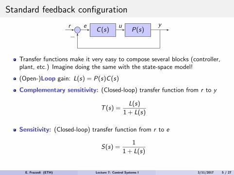
Transfer functions make it very easy to compose several blocks (controller,plant, etc.) Imagine doing the same with the state-space model!

(Open-)Loop gain: L(s) = P(s)C (s)

Complementary sensitivity: (Closed-loop) transfer function from r to y

T (s) =L(s)

1 + L(s)

Sensitivity: (Closed-loop) transfer function from r to e

S(s) =1

1 + L(s)


Concern #1: Well-posedness

D1 D2

r e u y

�

Assume both the plant and the controller are (static) gains.

Then the denominator of the closed-loop transfer functions would be1 +D2D1. If D2D1 = �1, the whole interconnections does not make sense —it is not well posed.

In general, never put in feedback blocks with a non-zero feed-through (i.e.,non-zero D term). It is always a pain to deal with (Matlab complains ofalgebraic loops), and in certain conditions can make the system ill-posed.


Concern #2: (Internal) Stability

It may be tempting to just check that the interconnection is I/O stable, i.e.,check that the poles of T (s) have negative real part.

However, consider what happens if C (s) = 1

s�1and P(s) = s�1

s+1:

The interconnection is I/O stable: T (s) = 1

s+2.

The closed-loop transfer function from r to u is unstable:S(s)C(s) = s+1

(s�1)(s+2).

While the system seems to be stable, internally the controller is blowing up.The pole-zero cancellation made the unstable controller mode unobservablein the interconnection.

Internal stability requires that all closed-loop transfer functions between anytwo signals must be stable.

Never be tempted to cancel an unstable pole with a non-minimum-phase zeroor viceversa.


How to determine closed-loop stability?

Assuming the feedback interconnection is well-posed and internally stable,then all that remains to do is to design C (s) in such a way that all the polesof T (s) have negative real part.

In principle one could just pick a trial design for C (s), go to matlab, andcheck what the closed-loop response (e.g., T (s)) looks like.

However, it is desired to find a systematic way to choose C (s), while doing aslittle calculations as possible. The first automatic control engineers wereworking with paper, pencil, and possibly a slide-rule.

All of classical control can be summarized in “exploit the knowledge of theloop gain L(s) to figure out the properties of the closed-loop transferfunctions T (s) and S(s) with the least e↵ort possible.”


Classical methods for feedback control

Remember: the main objective is to assess/design the properties of theclosed-loop system by exploiting the knowledge of the open-loop system, andavoiding complex calculations. We have three main methods:Root Locus

Quick assessment of control design feasibility. The insights are correct andclear.Can only be used for finite-dimensional systems (e.g. systems with a finitenumber of poles/zeros)Di�cult to do sophisticated design.Hard to represent uncertainty.

Nyquist plot

The most authoritative closed-loop stability test. It can always be used (finiteor infinite-dimensional systems)Easy to represent uncertainty.Di�cult to draw and to use for sophisticated design.

Bode plots

Potentially misleading results unless the system is open-loop stable andminimum-phase.Easy to represent uncertainty.Easy to draw, this is the tool of choice for sophisticated design.


Evan’s Root Locus method

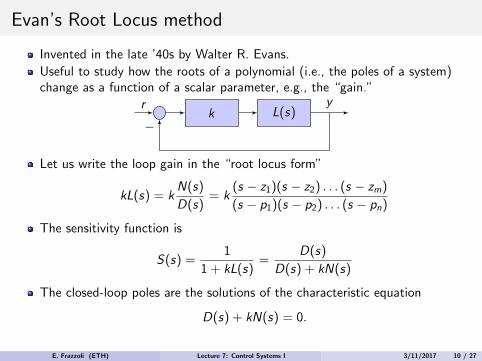
Invented in the late ’40s by Walter R. Evans.Useful to study how the roots of a polynomial (i.e., the poles of a system)change as a function of a scalar parameter, e.g., the “gain.”

k L(s)r y

�

Let us write the loop gain in the “root locus form”

kL(s) = kN(s)

D(s)= k

(s � z1)(s � z2) . . . (s � zm)

(s � p1)(s � p2) . . . (s � pn)

The sensitivity function is

S(s) =1

1 + kL(s)=

D(s)

D(s) + kN(s)

The closed-loop poles are the solutions of the characteristic equation

D(s) + kN(s) = 0.


The root locus rules

What can we say about the closed-loop poles?

Since the degree of D(s) + kN(s) is the same as the degree of D(s), thenumber of closed-loop poles is the same as the number of open-loop poles.

For k ! 0, D(s) + kN(s) ⇡ D(s), and the closed-loop poles approach theopen-loop poles.

For k ! 1, and the degree of N(s) is the same as the degree of D(s), then1

kD(s) + N(s) ⇡ N(s), and the closed-loop poles approach the open-loopzeros. If the degree of N(s) is smaller, then the “excess” closed-loop poles go“to infinity” (we will look into this more).

The closed-loop poles need to be symmetric wrt the real axis (i.e., either real,or complex-conjugate pairs).


The angle and magnitude rules

Let us rewrite the closed-loop characteristic equation as

N(s)

D(s)= � 1

k

The angle rule — Take the argument on both sides:

\(s � z1) + \(s � z2) + . . .+ \(s � zm)

�\(s � p1)�\(s � p2)� . . .�\(s � pn) =

⇢180�(±q 360�) if k > 00�(±q 360�) if k < 0

The magnitude rule — Take the argument on both sides:

|s � z1| · |s � z2| · . . . · |s � zm||s � p1| · |s � p2| · . . . · |s � pn|

=1

|k |


Graphical interpretation

All points on the complex plane that could potentially be a closed-loop pole(i.e., the root locus) have to satisfy the angle condition—which is essentiallyTHE rule for sketching the root locus.

Re

Ims

\s � p1

\s � p2

\s � z1

”The sum of the angles (counted from the real axis) from each zero to s,minus the sum of the angles from each pole to s must be equal to 180� (forpositive k) or 0� (for negative k), ± an integer multiple of 360�.”


All points on the real axis are on the root locus.

All points on the real axis to the left of an even number of poles/zeros (ornone) are on the negative k root locus

All points on the real axis to the right of an odd number of poles/zeros areon the positive k root locus.

When two branches come together on the real axis, there will be ‘breakaway”or “break-in” points.


Asymptotes

So what happens when k ! 1 and there are more open-loop poles thanzeros? We can see, e.g., from the magnitude condition, that the “excess”closed-loop poles will have to go to “to infinity”.Since this is the complex plane, we need to identify “in which direction” theygo towards infinity. This is were we use the angle rule again.If we “zoom out” su�ciently far, the contributions from all the finiteopen-loop poles and zeros will all be approximately equal to \s, and theangle rule is approximated by (m � n)\s = \� k ± q360�.In other words, as k ! 1, the excess poles will go to infinity alongasymptotes at angles of

\s = \� k ± q360�

m � n=

\� k ± q360�

n �m

These asymptotes meet in a “center of mass” lying on the real axis at

scom =

Pni=1

pi �Pm

j=1zj

n �m

(note that poles are “positive” unit masses, and zeros are “negative” unitmasses in this analogy)


Examples

k 1

s�1

r y

�

Re

Im


Examples

k1

(s�1)(s�2)

r y

�

Re

Im


Examples

k 1

s2+s+1

r y

�

Re

Im


Examples

k s+1

s2+s+1

r y

�

Re

Im


Examples

k1

(s+1)(s2+s+1)

r y

�

Re

Im


Examples

k s+1

s2+s+1

r y

�

Re

Im


Examples

k1

(s+1)(s2+s+1)

r y

�

Re

Im


Stabilizing an inverted pendulum

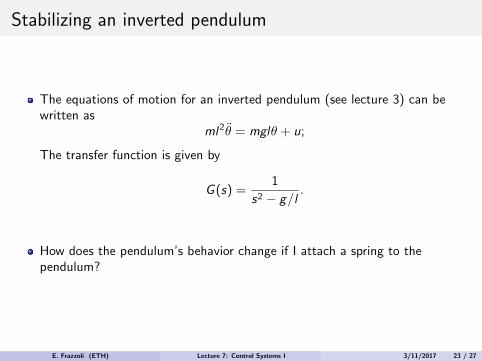
The equations of motion for an inverted pendulum (see lecture 3) can bewritten as

ml2✓ = mgl✓ + u;

The transfer function is given by

G (s) =1

s2 � g/l.

How does the pendulum’s behavior change if I attach a spring to thependulum?


Proportional control of an inverted pendulum

k1

s2�g/lr y

�

Re

Im


Proportional-derivative control of an inverted pendulum

kp + kd s1

s2�g/lr y

�

Re

Im


Root locus summary (for now)

Great tool for back-of-the-envelope control design, quick check forclosed-loop stability.

Qualitative sketches are typically enough. There are many detailed rules fordrawing the root locus in a very precise way: if you really need to do that,just use matlab or other methods.

Closed-loop poles start from the open loop poles, and are “repelled” by them.

Closed-loop poles are “attracted” by zeros (or go to infinity). Here you seean obvious explanation why non-minimum-phase zeros are in general to beavoided.

Remember that the root locus must be symmetric wrt the real axis.


Today’s learning objectives

Standard feedback control cofiguration and transfer function nomenclature

Well-posedness,

Internal vs. I/O stability

The root locus method.


Date post:	17-Mar-2018
Category:	Documents
Upload:	lamthu
View:	213 times
Download:	1 times

Control Systems I - ethz.ch · PDF fileControl Systems I Lecture 7: Feedback and the Root...

Documents