Abstract In this paper we study the controllability of an artificial advection–diffusion system through the boundary. Suitable Carleman estimates give us theobservability of the adjoint system in the one dimensional case. We also study somebasic properties of our problem such as backward uniqueness and we get an intuitiveresult on the control cost for vanishing viscosity.
P. CornilleauLycée du parc des Loges, 1, boulevard des Champs-Élysées,91012 Évry, Francee-mail: [email protected]
S. Guerrero (B)Laboratoire Jacques-Louis Lions, Université Pierre et Marie Curie,75252 Paris Cédex 05, Francee-mail: [email protected]
123
266 P. Cornilleau, S. Guerrero
0 Introduction
Artificial advection–diffusion problem In the present paper we deal with an advec-tion–diffusion problem with small viscosity truncated in one space direction. Ourinterest for the linear advection diffusion equation comes from the Navier–Stokesequations, but it arises also from other fields as, for example, meteorology. For a givenviscosity ε > 0, the incompressible Navier–Stokes equations can be written as
{ft + ( f.∇) f − ε� f + ∇ p = 0div( f ) = 0
where f is the velocity vector field, p the pressure, ∇ the gradient and � the usualLaplacian. Considering the flow around a body, we have that f is almost constant faraway from the body and equal to a. Then, our system can be approximated by theOseen equation
{ft + (a.∇) f − ε� f + ∇ p = 0div( f ) = 0
(see, for instance, [9, page 309, (1.2)]). Consequently, we get the following equationfor the vorticity u = rot( f )
ut + a.∇u − ε�u = 0.
In the sequel, we assume for simplicity that a is the nth unit vector of the canonicalbasis of Rn .
When one computes the solution of this problem, it can only be solved numericallyon a bounded domain. A good way to approximate the solution on the whole spacemay be given by the use of artificial boundary conditions (see [8,9]).
In this paper, we will consider an advection–diffusion system in a strip� := Rn−1×
(−L , 0) (L some positive constant) with particular artificial boundary conditions onboth sides of the domain. The following system was considered in [8, Section 6]:
⎧⎪⎪⎨⎪⎪⎩
ut + ∂xn u − ε�u =0 in (0, T )×�,
ε(ut + ∂νu) = 0 on (0, T )× �0,
ε(ut + ∂νu)+ u = 0 on (0, T )× �1,
u(0, .) = u0 in �,
(1)
where T > 0, �0 := Rn−1 × {0}, �1 := R
n−1 × {−L} and we have denoted ∂xn thepartial derivative with respect to xn and ∂ν the normal derivative. In [8, Theorem 3],the author proved that the solution of (1) converges in some sense to the restriction ofthe solution of
⎧⎨⎩
ut + ∂xn u = 0 in (0, T )× Rn−1 × R+,u = 0 on (0, T )× �1,
u(0, .) = u0 in Rn−1 × R+,
123
Controllability and observability 267
to (0, T )� (see also Section 6 in [8]).Up to our knowledge, there is no controllability result concerning system (1). In
this paper, we will be interested in the uniform boundary controllability of (1):
⎧⎨⎩
ut + ux − εuxx = 0 in (0, T )×�,
ε(ut + ∂νu)+ u1�1 = v1�i on (0, T )× ∂�,
u(0, .) = u0 in �,
where i = 0 or i = 1.In the sequel, we shall focus on the one-dimensional problem
(Sv)
⎧⎪⎪⎨⎪⎪⎩
ut + ux − εuxx = 0 in (0, T )× (−L , 0),ε(ut + ∂νu) = v on (0, T )× {0},ε(ut + ∂νu)+ u = 0 on (0, T )× {−L},u(0, .) = u0 in (−L , 0).
We are interested in the so-called null controllability of this system
for given u0,find v such that the solution of(Sv) satisfies u(T ) ≡ 0.
This property is classically equivalent to an observability inequality for the so-calledadjoint system (see Proposition 16 below for a proof), which can be written as
(S′)
⎧⎪⎪⎨⎪⎪⎩
ϕt + ϕx + εϕxx = 0 in (0, T )× (−L , 0),ε(ϕt − ∂νϕ)− ϕ = 0 on (0, T )× {0},ϕt − ∂νϕ = 0 on (0, T )× {−L},ϕ(T, .) = ϕT in (−L , 0).
The observability inequality corresponding to the previous controllability property is:
there exists C > 0 such that ‖ϕ(0, .)‖X ≤ C‖ϕ(., 0)‖L2(0,T ) ∀ϕT ∈ X, (2)
where the space X will be defined below. We refer the reader unfamiliar with the linksbetween observability and controllability to the seminal paper [4] (see also [10] onhyperbolic systems).
The phenomenon of degeneration of a parabolic problem to a hyperbolic one hasbeen studied in several papers: see, for instance, [2,6] (one dimensional heat equation)and [7] (Burgers equation). Similar results of interest can also be found in [1].
Main results We define X as the closure of D(�̄) := C∞(�̄) for the norm
‖u‖X := (‖u‖2L2(�)
+ ε‖u‖2L2(∂�)
)12 .
123
268 P. Cornilleau, S. Guerrero
Observe that X is the largest subspace of L2(�) such that its elements possess a tracein L2(∂�). In particular,
∀ε > 0, H1/2+ε(�) � X � L2(�).
We will denote by Cobs(ε) the cost of the null-control, which is the smallest con-stant C which fulfills the observability estimate (2). Our main result is the following:
Theorem 1 Assume T > 0.
• For any ε > 0, there exists C > 0 such that the solution of problem (S′) satisfies(2). Consequently, for every u0 ∈ X, there exists a control v ∈ L2(0, T ) with
‖v‖L2(0,T ) ≤ C‖u0‖X
such that the solution of the problem (Sv) satisfies u(T ) ≡ 0.• Furthermore, if T/L is large enough, the cost of the null-control Cobs(ε) tends to
zero exponentially as ε → 0:
∃C, k > 0 such that Cobs(ε) ≤ Ce−k/ε ∀ε ∈ (0, 1).
Remark 1 One can in fact obtain an observability result for the adjoint system atx = −L , that is
‖ϕ(0, .)‖X ≤ C‖ϕ(.,−L)‖L2(0,T ),
for any ϕ solution of (S′). This provides some controllability result for the directsystem on �1: a function v can be found depending continuously on u0 so that thesolution of
⎧⎪⎪⎨⎪⎪⎩
ut + ux − εuxx = 0 in (0, T )× (−L , 0),ut + ∂νu = 0 on (0, T )× {0},ε(ut + ∂νu)+ u = v on (0, T )× {−L},u(0, .) = u0 in (−L , 0),
satisfies u(T, .) ≡ 0. Despite the fact that it is more physical to control our system at�1, we have chosen to present here the result for the system (Sv) since its proof, lessobvious, requires more computations.
Remark 2 The fact that the control cost vanishes tells intuitively that the state is almostnull for T/L big enough. This is to be connected with the fact that, for ε = 0, thesystem is purely advective and then that, for T > L , its state is null.
In some context of inverse problems (be able to know the origin of a polluted riverfor instance), it can be interesting to know if the observation of the solution of thedirect problem (S0)
n on the boundary part �1 or �0 can allow us to recover the initialdata. The corresponding result is presented now and will be proved at the end of thefirst section.
123
Controllability and observability 269
Proposition 2 Let T > 0 and ε > 0. If the solution of (S0) with initial data u0 ∈ Xsatisfies u = 0 on (0, T ) × �1, then u0 ≡ 0. However, there is no constant C > 0such that the following estimate holds
‖u0‖X ≤ C‖u(.,−L)‖L2(0,T ) ∀u0 ∈ X. (3)
Remark 3 Using Remark 1, we can also obtain a similar result at x = 0.
The rest of the article is organized as follows: in the first section, we show the well-posedness of the direct and the adjoint problems using some semi-groups approach.In the second section, we adapt a Carleman inequality to the case of our one-dimen-sional problem. The third section is intended to explain how to get observability in theone-dimensional case and the equivalence between observability and controllability.
NotationsA � B means that, for some universal constant c > 0, A ≤ cB.A ∼ B means that, for some universal constant c > 1, c−1 B ≤ A ≤ cB.
1 Well-posedness and basic properties of systems
In this section, we work in dimension n.
1.1 Homogeneous problems
We will use some semi-group results to show existence and uniqueness of the homoge-neous direct problem (that is (S0)
n). This will enable to define solutions of the system(S0)
n as a semi-group value. We define H = (X, ‖.‖X ), V = H1(�) endowed withthe usual norm ‖.‖ and we consider the bilinear form on V defined by
a(u1, u2) = ε
∫�
∇u1.∇u2 +∫�
∂xn u1u2 +∫�1
u1u2. (4)
With the help of this bilinear form, one may now consider the space
D :={
u1 ∈ X; supu2∈D(�); ||u2||X ≤1
|a(u1, u2)| < +∞}
equipped with the natural norm
‖u1‖D = ‖u1‖X + supu2∈D(�); ||u2||X ≤1
|a(u1, u2)|.
123
270 P. Cornilleau, S. Guerrero
Note that, using an integration by parts, one shows that a(u1, u2) is well-defined foru1 ∈ X and u2 ∈ C∞(�) and that the map
u2 ∈ X → a(u1, u2) ∈ R
is well-defined and continuous for any u1 ∈ D.Using the Riesz representation theorem, we can define an operator A with domain
D(A) = D and such that
∀u1 ∈ D(A), ∀u2 ∈ X, 〈−Au1, u2〉X = a(u1, u2).
(S0)n might now be written in the following abstract way
{ut = Au,u(0, .) = u0,
since, for u ∈ C(R+,D(A)) ∩ C1(R+, X) a classical solution of (S0)n , we directly
get that
∀v ∈ X, 〈ut , v〉X = −a(u, v).
Proposition 3 Let ε > 0. Then A generates a continuous semi-group (etA)t≥0 on X.
Proof Using the Hille–Yoshida theorem, it is sufficient to show that A is a maximalmonotone operator.
• First, Green–Riemann formula gives
〈Au, u〉X = −ε∫�
|∇u|2 − 1
2
∫∂�
|u|2,
so the monotonicity is proved.• Given v ∈ X , we have to solve (I − A)u = v, that is to find u ∈ D(A) such that
∀u′ ∈ X, 〈(I − A)u, u′〉X = 〈v, u′〉X .
The left-hand side term of this equation is a continuous bilinear form B on the spaceV while the right-hand side term is a continuous linear form L on V . Moreover,using (4), we can easily compute
B(u, u) = ‖u‖2X + ε
∫�
|∇u|2 + 1
2
∫∂�
|u|2 ≥ min{1, ε}‖u‖2,
which show that B is coercive on V . Consequently, Lax–Milgram theorem showsthat there exists u ∈ V such that B(u, u′) = L(u′), ∀u′ ∈ V . Using test functionsu′ ∈ D(�) additionally gives u ∈ D(A) and our proof ends. ��
123
Controllability and observability 271
In particular, for every initial data u0 ∈ X , we have existence and uniqueness of asolution u ∈ C(R+, X) to (S0)
n . We will call these solutions weak solutions opposedto strong solutions i.e. such that u0 ∈ D(A) and which fulfill u ∈ C(R+,D(A)) ∩C1(R+, X). One can notice that, using the density of D(A) in X , a weak solution canalways be approximated by a strong solution.
Let us introduce the adjoint system in dimension n
(S′)n
⎧⎪⎪⎨⎪⎪⎩
ϕt + ∂xnϕ + ε�ϕ = 0 in (0, T )×�,
ε(ϕt − ∂νϕ)− ϕ = 0 on (0, T )× �0,
ϕt − ∂νϕ = 0 on (0, T )× �1,
ϕ(T, .) = ϕT in �.
Defining the adjoint A∗ of A, we can show in a similar way as before that (S′)n maybe written in the following abstract way
{ϕt + A∗ϕ = 0,ϕ(T, .) = ϕT .
The adjoint operator A∗ is also a maximal monotone operator with domain D(A∗).Thus, for every initial data ϕT ∈ X , we have existence and uniqueness of a solutionϕ ∈ C(R+, X) to (S′)n given by means of the backward semi-group (e(T −t)A∗
)t≥0.We will also speak of weak solutions or strong solutions in this situation.
1.2 Nonhomogeneous direct problems
We consider a slightly more general system
(S f,g0,g1)n
⎧⎪⎪⎨⎪⎪⎩
ut + ∂xn u − ε�u = f in (0, T )×�,
ε(ut + ∂νu) = g0 on (0, T )× �0,
ε(ut + ∂νu)+ u = g1 on (0, T )× �1,
u(0, .) = u0 in �,
with f ∈ L2((0, T ) × �), g0 ∈ L2((0, T ) × �0) and g1 ∈ L2((0, T ) × �1). Weconsider a function g on ∂� such that g = gi on �i (i = 0, 1).
Definition 4 We say that u ∈ C([0, T ] , X) is a transposition solution of (S f,g0,g1)n
if, for every function ϕ ∈ C([0, T ],D(A∗)) ∩ C1([0, T ], X), the following identityholds
where we have defined, using the Riesz representation theorem, F(t) ∈ X such that
〈F(t), u′〉X =∫�
f (t)u′ +∫∂�
g(t)u′, ∀u′ ∈ X. (5)
Proposition 5 Let T > 0, u0 ∈ X, f ∈ L2((0, T )×�), g0 ∈ L2((0, T )× �0) andg1 ∈ L2((0, T )× �1). Then (S f,g0,g1)
n possesses a unique solution u.
Proof Let us first assume that u belongs to u ∈ C([0, T ],D(A))∩C1([0, T ], X). Then,it is easy to prove that u is a solution to (S f,g0,g1)
n if and only if, for any φ ∈ D(A∗),
〈ut , φ〉X = 〈u,A∗φ〉X + 〈F, φ〉X in [0, T ].
Consequently, thanks to Duhamel formula, u is a solution of (S f,g0,g1)n is equivalent
to
u(t) = etAu0 +t∫
0
e(t−s)AF(s)ds, ∀t ∈ [0, T ],
since D(A∗) is dense in X .In order to prove the existence of a solution u ∈ C([0, T ], X), we approximate
(u0, f, g) by
(u p0 , f p, g p
0 , g p1 ) ∈ D(A)× C([0, T ], L2(�))
×C([0, T ], L2(�0))× C([0, T ], L2(�1))
in
X × L2((0, T ), L2(�))× L2((0, T ), L2(�0))× L2((0, T ), L2(�1)).
Then, we know that u p given by
u p(t) = etAu p0 +
t∫0
e(t−s)AF p(s) ds, ∀t ∈ [0, T ],
where F p is related to ( f p, g p0 , g p
1 ) by formula (5), is the solution of (S f p,g p0 ,g
p1)n .
Passing to the limit in this identity, we get that u p → u in C([0, T ], X) with
u(t) := etAu0 +t∫
0
e(t−s)AF(s) ds, ∀t ∈ [0, T ].
Furthermore, passing to the limit in Definition 4 for u p, we obtain that u is a solutionof (S f,g0,g1)
n . Moreover, this argument also proves the uniqueness of the solution. ��
123
Controllability and observability 273
We now focus on some regularization effect for our general system and for some tech-nical reasons we want to have some explicit dependence of the bounds on ε. For thisresult, it is essential that ε > 0.
Lemma 6 Let ε ∈ (0, 1), f ∈ L2((0, T ) × �), g0 ∈ L2((0, T ) × �0) and g1 ∈L2((0, T )× �1).
• Let u0 ∈ X. Then if u is the solution of (S f,g0,g1)n, u belongs to L2((0, T ), H1(�))∩
ε1/2 (‖u0‖H1(�) + ‖ f ‖L2((0,T )×�) + ‖g‖L2((0,T )×∂�)),
(7)
where C > 0 only depends on T .
Proof Approximating u by a regular function (in L2((0, T ),D(�))), all computationsbelow are justified.
• First, we multiply our main equation by u and we integrate on �. An applicationof Green–Riemann formula with use of the boundary conditions gives the identity
1
2
d
dt‖u‖2
X + 1
2
∫∂�
|u|2 + ε
∫�
|∇u|2 =∫�
f u +∫∂�
gu,
which immediately yields
d
dt‖u‖2
X +∫∂�
|u|2 + 2ε∫�
|∇u|2 ≤ ‖u‖2X + ‖ f ‖2
L2(�)+ ‖g‖2
L2(∂�).
Finally, Gronwall’s lemma yields (6).• Now, we multiply the main equation by ut and we integrate on �, which, using
Green–Riemann formula and the boundary conditions provide the identity
‖ut‖2X +
∫�
∂xn uut + ε
2
d
dt
⎛⎝∫�
|∇u|2⎞⎠ + 1
2
d
dt
⎛⎜⎝
∫�1
|u|2⎞⎟⎠ =
∫�
f ut +∫∂�
gut ,
123
274 P. Cornilleau, S. Guerrero
Now
−∫�
ut∂xn u � 1
2
∫�
|∇u|2 + 1
2‖ut‖2
X
and, using again Young’s inequality, we have
∫�
f ut +∫∂�
gut � 1
4‖ut‖2
X + C(‖ f ‖2
L2(�)+ ‖g‖2
L2(∂�)
).
We have thus proven the following inequality
‖ut‖2X + 2ε
d
dt
⎛⎝∫�
|∇u|2⎞⎠
+ 2d
dt
∫�1
|u|2 ≤ 2∫�
|∇u|2 + C(‖g‖2
L2(∂�)+ ‖ f ‖2
L2(�)
). (8)
We integrate here between 0 and t and estimate the first term in the right-hand sideusing (6) to get
∫�
|∇u|2 � C
ε2
⎛⎝
T∫0
(‖ f (t)‖2L2(�)
+ ‖g(t)‖2L2(∂�)
) dt + ‖u0‖2H1(�)
⎞⎠ ,
for t ∈ (0, T ). We now inject this into (8) to get the second part of the requiredresult
‖ut‖2L2((0,T );X) � C
ε
⎛⎝
T∫0
(‖ f (t)‖2L2(�)
+ ‖g(t)‖2L2(∂�)
)dt + ‖u0‖2H1(�)
⎞⎠ .
Writing the problem as
⎧⎨⎩
−�u = 1ε( f − ut − ∂xn u) in (0, T )×�,
∂νu = g0ε
− ut on (0, T )× �0,
∂νu = g1ε
− ut − 1εu on (0, T )× �1,
we get that u ∈ L2((0, T ),D(A)) and the existence of some constant C > 0 suchthat
which gives the last part of the required result (7). ��Remark 4 Working on the non-homogeneous adjoint problem and using the backwardsemi-group e(T −t)A∗
, one is able to show that the estimates of Lemma 6 hold for thesystem
(S′f,g0,g1
)n
⎧⎪⎪⎨⎪⎪⎩
ϕt + ∂xnϕ + ε�ϕ = f in (0, T )×�,
ε(ϕt − ∂νϕ)− ϕ = g0 on (0, T )× �0,
ε(ϕt − ∂νϕ) = g1 on (0, T )× �1,
ϕ(T, .) = ϕT in �.
1.3 Backward uniqueness
We will show here the backward uniqueness of systems (S0)n and (S′)n for ε > 0,
thanks to the well-known result of Lions–Malgrange [12] and the regularization effect.
Lemma 7 Let u0 ∈ X and δ ∈ (0, T ). Then, the solution u of (S0)n satisfies u ∈
C([δ, T ],D(A)).Proof Our strategy is to show that u ∈ L2((δ, T ); H2(�)) and ut ∈ L2((δ, T ); H2(�)).This easily implies that u ∈ C([δ, T ]; H2(�)).
We first select some regular cut-off function θ1 such that θ1 = 1 on (δ/2, T ) andθ1 = 0 on (0, δ/4). If u1 = θ1u, we have that
⎧⎪⎪⎨⎪⎪⎩
u1,t + ∂xn u1 − ε�u1 = θ ′1u in (0, T )×�,
ε(u1,t + ∂νu1) = εθ ′1u on (0, T )× �0,
ε(u1,t + ∂νu1)+ u1 = εθ ′1u on (0, T )× �1,
u1(0, .) = 0 in �,
that is u1 satisfies (Sθ ′1u,εθ ′
1u,εθ ′1u)
n . An application of Lemma 6 gives that u1 ∈L2((0, T ),D(A)) and u1,t ∈ L2((0, T ), X). This implies in particular that u ∈L2((δ, T ),D(A)).
We now focus on ut and we select another cut-off function θ2 such that θ2 = 1 on(δ, T ) and θ2 = 0 on (0, δ/2). We write the system satisfied by θ2u and we differentiateit with respect to time. One deduces that u2 = (θ2u)t is the solution of
(Sθ ′2ut +θ ′′
2 u,ε(θ ′2ut +θ ′′
2 u),ε(θ ′2ut +θ ′′
2 u))n .
Using that |θ ′2| � |θ1|, Lemma 6 gives that u2 ∈ L2((0, T ),D(A)) that is ut ∈
L2((δ, T ),D(A)). ��Proposition 8 Assume that u is a weak solution of (S0)
n such that u(T ) = 0. Thenu0 ≡ 0.
Proof If 0 < δ < T , then Lemma 7 shows that u(δ) ∈ D(A). We will now applyThéorème 1.1 of [12] to u as a solution of (S0)
n in the time interval (δ, T ) to show
123
276 P. Cornilleau, S. Guerrero
that u(δ, .) = 0. The bilinear form a defined in (4) can be split into two bilinear formson V defined by
a(u1, u2) = a0(t, u1, u2)+ a1(t, u1, u2)
with
a0(t, u1, u2) = ε
∫�
∇u1.∇u2, a1(t, u1, u2) =∫�
∂xn u1u2 +∫�1
u1u2.
The first four hypotheses in [12] (see (1.1)–(1.4) in that reference) are satisfied sinceu ∈ L2(δ, T ; V ) ∩ H1(δ, T ; H) (from Lemma 6 above), u(t) ∈ D(A) for almostevery t ∈ (δ, T ), ut = Au and u(T, .) ≡ 0. On the other hand, it is clear that a0 anda1 are continuous bilinear forms on V and that they do not depend on time t . It is alsostraightforward to see that
∀u ∈ V, a0(t, u, u)+ ‖u‖2X � min{1, ε}‖u‖2
and, for some constant C > 0,
∀u, v ∈ V, |a1(t, u1, u2)| � C‖u1‖‖u2‖X .
This means that Hypothesis I in that reference is fulfilled. We have shown that u(δ, .)=0, which finishes the proof since
u0 = limδ→0
u(δ) = 0.
��Remark 5 The result also holds for the adjoint system: if ϕ is a weak solution of (S′)nsuch that ϕ(0) ≡ 0 then ϕT = 0. The proof is very similar to the one above and is leftto the reader.
1.4 Proof of Proposition 2
The fact that u = 0 on (0, T )× �1 implies u0 ≡ 0 is a straightforward consequenceof the backward uniqueness of system (S0)
n . Indeed, similarly as (2), we can provethe observability inequality
‖u(T, .)‖X � ‖u‖L2((0,T )×�1),
(see Remark 6 below), which combined with Proposition 8 gives u0 ≡ 0.To show that (3) is false, we first need to prove some well-posedness result of (S0)
n
with u0 in a less regular space. For s ∈ (0, 1/2), we define Xs as the closure of D(�̄)
123
Controllability and observability 277
for the norm
‖u‖Xs := (‖u‖2Hs (�) + ε‖u‖2
Hs (∂�))12 ,
where Hs(�) (resp. Hs(∂�)) stands for the usual Sobolev space on � (resp. ∂�).One easily shows that Xs is a Hilbert space. We now denote X−s the set of functionsu2 such that the linear form
u1 ∈ D(�̄) −→ 〈u1, u2〉X
can be extended in a continuous way on Xs . If u1 ∈ X−s , u2 ∈ Xs we denote thisextension by 〈u1, u2〉−s,s .
If u0 ∈ X−s , we say that u is a solution by transposition of (S0)n if, for every
f ∈ L2((0, T )×�)
T∫0
∫�
u f + 〈u0, ϕ(0, .)〉−s,s = 0,
where ϕ is the weak solution (see Remark 4) of
(S′f,0,0)
n
⎧⎪⎪⎨⎪⎪⎩
ϕt + ∂xnϕ + ε�ϕ = f in (0, T )×�,
ε(ϕt − ∂νϕ)− ϕ = 0 on (0, T )× �0,
ϕt − ∂νϕ = 0 on (0, T )× �1,
ϕ(T, .) = 0 in �.
Using the Riesz representation theorem and continuity (see Remark 4) of
f ∈ L2((0, T )×�) −→ ϕ(0, .) ∈ H1(�),
it is obvious that, for any u0 ∈ X−s , there exists a solution by transposition of (S0)n ,
u ∈ L2((0, T )×�), such that
‖u‖L2((0,T )×�) � ‖u0‖X−s .
Moreover, if u0 ∈ X = X0, Lemma 6 shows that the solution u satisfies
‖u‖L2((0,T ),H1(�)) � ‖u0‖X0 .
If one uses classical interpolation results (see [11]), we can deduce that for everyθ ∈ (0, 1/2), for any u0 ∈ X−sθ = [X, X−s]1−θ , there exists a solution u ∈L2((0, T ), H1−θ (�)) such that
‖u‖L2((0,T ),H1−θ (�)) � ‖u0‖X−sθ .
123
278 P. Cornilleau, S. Guerrero
Using classical trace result, we have that
‖u‖L2((0,T )×∂�) � ‖u0‖X−sθ . (9)
On the other hand, estimate (3) implies in particular that
‖u0‖X � ‖u‖L2((0,T )×�1)∀u0 ∈ D(�). (10)
Finally, (9) and (10) yields the contradictory inclusion X−sθ ↪→ X . ��
2 Carleman inequality in dimension 1
In this paragraph, we will establish a Carleman-type inequality keeping track of theexplicit dependence of all the constants with respect to T and ε. As in [5], we introducethe following weight functions:
where λ > e2L .The rest of this paragraph will be dedicated to the proof of the following inequality:
Theorem 9 There exists C > 0 and s0 > 0 such that for every ε ∈ (0, 1) and everys � s0(εT + ε2T 2) the following inequality is satisfied for every ϕT ∈ X :
s3∫
(0,T )×(−L ,0)
φ3e−2sα|ϕ|2 + s∫
(0,T )×(−L ,0)
φe−2sα|ϕx |2
+s3∫
(0,T )×{0,−L}φ3e−2sα|ϕ|2 � Cs7
∫(0,T )×{0}
e−4sα+2sα(.,−L)φ7|ϕ|2. (11)
Here, ϕ stands for the solution of (S′) associated to ϕT .
Remark 6 One can in fact obtain the following Carleman estimate with control termin �1
s3∫
(0,T )×(−L ,0)
φ3e−2sα|ϕ|2 + s∫
(0,T )×(−L ,0)
φe−2sα|ϕx |2
+s3∫
(0,T )×{0,−L}φ3e−2sα|ϕ|2 � Cs7
∫(0,T )×{−L}
e−4sα+2sα(.,0)φ7|ϕ|2.
simply by choosing the weight function η(x) equal to x → −x + L . The proof is verysimilar and the sequel will show how to deal with this case too.
123
Controllability and observability 279
In order to perform a Carleman inequality for system (S′), we first do a scaling in time.Introducing T̃ := εT , ϕ̃(t, x) := ϕ(t/ε, x) and the weights α̃(t, x) := α(t/ε, x),φ̃(t, x) := φ(t/ε, x); we have the following system
⎧⎪⎪⎨⎪⎪⎩
ϕ̃t + ε−1ϕ̃x + ϕ̃xx = 0 in q,ε2(ϕ̃t − ε−1∂νϕ̃)− ϕ̃ = 0 on σ0,
ϕ̃t − ε−1∂νϕ̃ = 0 on σ1,
ϕ̃|t=T̃ = ϕT in (−L , 0).
(12)
if q := (0, T̃ ) × (−L , 0), σ := (0, T̃ ) × {−L , 0}, σ0 := (0, T̃ ) × {0} and σ1 :=(0, T̃ )× {−L}. We will now explain how to get the following result.
Proposition 10 There exists C > 0, such that for every ε ∈ (0, 1) and every s �C(T̃ + ε−1T̃ 2 + ε1/3T̃ 2/3), the following inequality is satisfied for every solution of(12) associated to ϕ̃T ∈ X :
s3∫q
φ̃3e−2sα̃|ϕ̃|2 + s∫q
φ̃e−2sα̃|ϕ̃x |2 + s3∫σ
φ̃3e−2sα̃|ϕ̃|2
� Cs7∫σ0
e−4sα̃+2sα̃(.,−L)φ̃7|ϕ̃|2. (13)
Observe that Proposition 10 directly implies Theorem 9.All along the proof we will need several properties of the weight functions:
• α̃x = −φ̃, α̃xx = −φ̃.There are essentially two steps in this proof:
– The first one consists in doing a Carleman estimate similar to that of [5]. The idea isto compute the L2 product of some operators applied to e−sα̃ ϕ̃, do integrations byparts and make a convenient choice of the parameter s. This will give an estimatewhere we still have a boundary term on σ0 in the right-hand side.
– In the second one, we will study the boundary terms appearing in the right handside due to the boundary conditions. We will perform the proof of this theorem forsmooth solutions, so that the general proof follows from a density argument.
The big difference with general parabolic equations is the special boundary condition.Up to our knowledge, no Carleman inequalities have been performed when the partialtime derivative appears on the boundary condition. The fact that we still have a Carl-eman inequality for our system comes from the fact that our system remains somehowparabolic.
We will first estimate the left hand side terms of (13) like in the classical Carlemanestimate (see [5]). We obtain:
123
280 P. Cornilleau, S. Guerrero
Proposition 12 There exists C > 0, such that for every ε ∈ (0, 1) and every s �C(T̃ + ε−1T̃ 2 + ε1/3T̃ 2/3), the following inequality is satisfied for every solution of(12) associated to ϕ̃T ∈ X :
s3∫q
φ̃3e−2sα̃|ϕ̃|2 + s2∫q
φ̃e−2sα̃|ϕ̃x |2 + s−1∫q
φ̃−1e−2sα̃(|ϕ̃xx |2 + |ϕ̃t |2)
+ s3∫σ1
φ̃3e−2sα̃|ϕ̃|2 � s5∫σ0
φ̃5e−2sα̃|ϕ̃|2 + ε2s∫σ0
φ̃e−2sα̃|ϕ̃t |2. (14)
Proof Let us introduceψ := ϕ̃e−sα̃ . We state the equations satisfied byψ . In (0, T̃ )×(−L , 0), we have the identity
P1ψ + P2ψ = P3ψ,
where
P1ψ = ψt + 2sα̃xψx + ε−1ψx , (15)
P2ψ = ψxx + s2α̃2xψ + sα̃tψ + ε−1sα̃xψ, (16)
and
P3ψ = −sα̃xxψ.
On the other hand, the boundary conditions are:
ε2(ψt + sα̃tψ − ε−1(ψx + sα̃xψ))− ψ = 0 on x = 0, (17)
ε(ψt + sα̃tψ)+ ψx + sα̃xψ = 0 on x = −L . (18)
We take the L2 norm in both sides of the identity in q:
‖P1ψ‖2L2(q) + ‖P2ψ‖2
L2(q) + 2(P1ψ, P2ψ)L2(q) = ‖P3ψ‖2L2(q). (19)
Using Lemma 11, we directly obtain
‖ P3ψ‖2L2(q) � s2
∫q
φ̃2|ψ |2.
We focus on the expression of the double product (P1ψ, P2ψ)L2(q). This productcontains 12 terms which will be denoted by Ti j (ψ) for 1 � i � 3, 1 � j � 4. Westudy them successively.
123
Controllability and observability 281
• An integration by parts in space and then in time shows that, since ψ(0, .)= ψ(T̃ , .) = 0, we have
T11(ψ) =∫q
ψtψxx = −1
2
∫q
(|ψx |2)t +∫σ0
ψxψt −∫σ1
ψxψt
=∫σ0
ψxψt −∫σ1
ψxψt .
Now, we use the boundary condition (17). We have
∫σ0
ψxψt � ε
∫σ0
|ψt |2 − εT̃ 2s∫σ0
φ̃3|ψ |2 − T̃ s∫σ0
φ̃2|ψ |2.
Thanks to the fact thatψ(0, .) = ψ(T̃ , .) = 0, the same computations can be doneon x = −L using (18) so we obtain the following for this term:
T11(ψ) � −εT̃ 2s∫σ
φ̃3|ψ |2 − T̃ s∫σ
φ̃2|ψ |2.
• Integrating by parts in time, we find
T12(ψ) = s2
2
∫q
α̃2x (|ψ |2)t = −s2
∫q
α̃x α̃xt |ψ |2,
T13(ψ) = s
2
∫q
α̃t (|ψ |2)t = − s
2
∫q
α̃t t |ψ |2,
T14(ψ) = ε−1 s
2
∫q
α̃x (|ψ |2)t = −ε−1 s
2
∫q
α̃t x |ψ |2,
and using Lemma 11, we get
T12(ψ) � −T̃ s2∫q
φ̃3|ψ |2,
T13(ψ) � −T̃ 2s∫q
φ̃3|ψ |2,
T14(ψ) � −ε−1T̃ s∫q
φ̃2|ψ |2.
123
282 P. Cornilleau, S. Guerrero
• Now, integrating by parts in space, we have
T21(ψ) = s∫q
α̃x (|ψx |2)x = −s∫q
α̃xx |ψx |2 + s∫σ0
α̃x |ψx |2 − s∫σ1
α̃x |ψx |2.
Thanks to Lemma 11 (the choice of η is important here), the last term is positive.Using the boundary condition (17) and Lemma 11, we finally get
T21(ψ) � s∫q
φ̃|ψx |2 − s3∫σ0
φ̃3|ψ |2 − ε2s3T̃ 2∫σ0
φ̃5|ψ |2
+ s∫σ1
φ̃|ψx |2 − ε2s∫σ0
φ̃|ψt |2.
• An integration by parts in space provides
T22(ψ)=s3∫q
α̃3x (|ψ |2)x =−3s3
∫q
α̃2x α̃xx |ψ |2 + s3
∫σ0
α̃3x |ψ |2 − s3
∫σ1
α̃3x |ψ |2.
This readily yields
T22(ψ) � s3∫q
φ̃3|ψ |2 + s3∫σ1
φ̃3|ψ |2 − s3∫σ0
φ̃3|ψ |2.
• Again an integration by parts in space gives
T23(ψ) = s2∫q
α̃t α̃x (|ψ |2)x
= −s2∫q
(α̃t α̃x )x |ψ |2 + s2∫σ0
α̃t α̃x |ψ |2 − s2∫σ1
α̃t α̃x |ψ |2.
Using Lemma 11, we obtain
T23(ψ) � −s2T̃∫q
φ̃3|ψ |2 − s2T̃∫σ0
φ̃3|ψ |2 − s2T̃∫σ1
φ̃3|ψ |2.
• The last integral concerning the second term in the expression of P1ψ is
T24(ψ) = ε−1s2∫q
α̃2x (|ψ |2)x .
123
Controllability and observability 283
After an integration by parts in space, we get
T24(ψ) ≥ −2ε−1s2∫q
φ̃2|ψ |2 − ε−1s2∫σ1
φ̃2|ψ |2.
• We consider now the third term in the expression of P1ψ . We have
T31(ψ) = ε−1
2
∫q
(|ψx |2)x ≥ −ε−1
2
∫σ1
|ψx |2.
• Now, we integrate by parts with respect to x and we have
T32(ψ) = ε−1
2s2
∫q
α̃2x (|ψ |2)x ≥ −ε−1s2
∫q
α̃x α̃xx |ψ |2 − ε−1
2s2
∫σ1
α̃2x |ψ |2
≥ −ε−1s2∫q
φ̃2|ψ |2 − ε−1
2s2
∫σ1
φ̃2|ψ |2.
• Then, using another integration by parts in x we obtain
T33(ψ) = ε−1
2s∫q
α̃t (|ψ |2)x � −ε−1sT̃∫q
φ̃2|ψ |2
−ε−1T̃ s∫σ1
φ̃2|ψ |2 − ε−1T̃ s∫σ0
φ̃2|ψ |2.
• Finally, arguing as before, we find
T34(ψ) = ε−2
2s∫q
α̃x (|ψ |2)x ≥ ε−2
2s2
∫q
φ̃|ψ |2 − Cε−2s∫σ0
φ̃|ψ |2
� −ε−2s∫σ0
φ̃|ψ |2.
Putting together all the terms and combining the resulting inequality with (19), weobtain
Let us now see that we can absorb some right hand side terms with the help of theparameter s.
• First, we see that the distributed terms in J1(ψ) can be absorbed by the first termin the definition of I1(ψ) for a choice of s � ε−1/2T̃ 3/2 + ε−1T̃ 2.
• Second, we use the second term of I1(ψ) in order to absorb the integrals in thesecond line of the definition of J1(ψ). We find that this can be done as long ass � ε−1T̃ 2 + ε−1/2T̃ 3/2 since ε < 1.
• Next, we observe that, provided s � ε−1T̃ 2, the second term in J2(ψx ) absorbsJ3(ψx ).
Moreover, we observe that all the control terms can be bounded in the following way:
|L(ψ)| � s5∫σ0
φ̃5|ψ |2
as long as s � T̃ (1 + ε−1T̃ ), using that ε < 1.
123
Controllability and observability 285
Next, we use the expression of P1ψ and P2ψ [see (15), (16)] in order to obtainsome estimates for the terms ψt and ψxx respectively:
s−1∫q
φ̃−1|ψt |2 � s2∫q
φ̃|ψx |2 + s−1ε−2∫q
φ̃−1|ψx |2 + s−1∫q
φ̃−1|P1ψ |2
� s2∫q
φ̃|ψx |2 +∫q
|P1ψ |2
for any s � ε−1T̃ 2 and
s−1∫q
φ̃−1|ψxx |2 � s3
T̃∫0
0∫−L
φ̃3|ψ |2 + sT̃ 2∫q
φ̃3|ψx |2 + ε−2s2∫q
φ̃|ψ |2
+ s−1∫q
φ̃−1|P2ψ |2 � s3∫q
φ̃3|ψ |2+s2∫q
φ̃|ψx |2+∫q
|P2ψ |2,
for s � T̃ + ε−1T̃ 2.Combining all this with (20), we obtain
s∫q
φ̃(s2φ̃2|ψ |2 + |ψx |2)+ s−1∫q
φ̃−1(|ψxx |2 + |ψt |2)+ s3∫σ1
φ̃3|ψ |2
� s5∫σ0
φ̃5|ψ |2 + ε2s∫σ0
φ̃|ψt |2, (21)
for s � T̃ (1 + ε−1T̃ ).Finally, we come back to our variable ϕ̃. We first remark thatψx = e−sα̃(ϕ̃x +sφ̃ϕ̃)
and so
s∫q
φ̃e−2sα̃|ϕ̃x |2 � s∫q
φ̃|ψx |2 + s3∫q
φ̃3|ψ |2.
Then, we have that ψt = e−sα̃(ϕ̃t − sα̃t ϕ̃), hence
s−1∫q
φ̃−1e−2sα̃|ϕ̃t |2 � s−1∫q
φ̃−1|ψt |2 + sT̃ 2∫q
φ̃3|ψ |2 � s−1∫q
φ̃−1|ψt |2
+ s3∫q
φ̃3|ψ |2
123
286 P. Cornilleau, S. Guerrero
for s � T̃ . Analogously, we can prove that
s−1
T̃∫0
∫q
φ̃−1e−2sα̃|ϕ̃xx |2 � s−1∫q
φ̃−1|ψxx |2 + s3∫q
φ̃3|ψ |2 + s2∫q
φ̃|ψx |2,
for s � T̃ 2.We combine this with (21) and we obtain the required result
s3∫q
φ̃3e−2sα̃|ϕ̃|2 + s∫q
φ̃e−2sα̃|ϕ̃x |2 + s−1∫q
φ̃−1e−2sα̃(|ϕ̃xx |2 + |ϕ̃t |2)
+s3∫σ1
φ̃3e−2sα̃|ϕ̃|2 � s5∫σ0
φ̃5e−2sα̃|ϕ̃|2 + ε2s∫σ0
φ̃e−2sα̃|ϕ̃t |2, (22)
for s � T̃ (1 + ε−1T̃ )+ ε1/3T̃ 2/3 and using that
ε2s3T̃ 2∫σ0
φ̃5e−2sα̃|ϕ̃|2 � s5∫σ0
φ̃5e−2sα̃|ϕ̃|2
which is true for s � T̃ (recall that ε < 1). ��With this result, we will now finish the proof of Proposition 10.
Estimate of the boundary term In this paragraph we will estimate the boundary term
ε2s∫σ0
φ̃e−2sα̃|ϕ̃t |2.
After an integration by parts in time, we get
ε2s∫σ0
φ̃e−2sα̃|ϕ̃t |2 = ε2
2s∫σ0
(φ̃e−2sα̃)t t |ϕ̃|2 − ε2s∫σ0
φ̃e−2sα̃ ϕ̃ ϕ̃t t
� T̃ 2ε2s3∫σ0
φ̃5e−2sα̃|ϕ̃|2 + ε2s∫σ0
φ̃e−2sα̃|ϕ̃| |ϕ̃t t |, (23)
for s � T̃ + T̃ 2. In order to estimate the second time derivative at x = 0, we will applysome a priori estimates for the adjoint system. Indeed, let us consider the followingfunction
Using Remark 4 for (t, x) −→ ζ(εt, x) we find in particular
ε
∫σ
|ζt |2 �∫q
|θt |2|ϕ̃t |2 + ε2∫σ
(θt )2|ϕ̃t |2.
This directly implies that
ε
∫σ
θ2|ϕ̃t t |2 �∫q
|θt |2|ϕ̃t |2 + ε2∫σ
(θt )2|ϕ̃t |2.
Integrating by parts in time in the last integral, we have
ε
∫σ
θ2|ϕ̃t t |2 �
⎛⎝∫
q
|θt |2|ϕ̃t |2 + ε2∫σ
((θt )2)t t |ϕ̃|2 + ε3
∫σ
(θt )4θ−2|ϕ̃|2
⎞⎠
+ε2
∫σ
θ2|ϕ̃t t |2.
From the definition of θ(t) and multiplying the previous inequality by s−3, we findthat (since ε < 1)
ε s−3∫σ
(e−2sα̃ φ̃−5)(.,−L)|ϕ̃t t |2
� T̃ 2
⎛⎝s−1
∫q
φ̃−1e−2sα̃|ϕ̃t |2 + ε2T̃ 2s∫σ
(φ̃3e−2sα̃)(.,−L)|ϕ̃|2⎞⎠
� T̃ 2
⎛⎝s−1
∫q
φ̃−1e−2sα̃|ϕ̃t |2 + s3∫σ
(φ̃3e−2sα̃)(.,−L)|ϕ̃|2⎞⎠ (24)
123
288 P. Cornilleau, S. Guerrero
for s � εT̃ . Using Cauchy–Schwarz inequality in the last term of the right hand sideof (23), we obtain
ε2s∫σ0
φ̃e−2sα̃|ϕ̃| |ϕ̃t t | � εT̃ −2s−3∫σ
(e−2sα̃ φ̃−5)(.,−L)|ϕ̃t t |2
+ε3T̃ 2s5∫σ0
e−4sα̃+2sα̃(.,−L)φ̃7|ϕ̃|2
Combining this with (24) and (22) yields the desired inequality (13). ��
3 Observability and control
In this section, we prove Theorem 1.
3.1 Dissipation and observability result
Our first goal, as in [2], will be to get some dissipation result. Even if we will only usethis result in dimension one, we present it in dimension n for the sake of completeness(see also [3]).
Proposition 13 For every ε ∈ (0, 1), for every time t1, t2 > 0 such that t2 − t1 > Land for every weak solution ϕ of (S′)n, the following estimate holds
‖ϕ(t1)‖X � exp
{− (t2 − t1 − L)2
4ε(t2 − t1)
}‖ϕ(t2)‖X .
Proof We first consider a weight function ρ(t, x) = exp( rε
xn) for some constantr ∈ (0, 1) which will be fixed later. We will first treat the strong solutions case and,using a density argument, we will get the weak solutions case.
We multiply the equation satisfied by ϕ by ρϕ and we integrate on �. We get thefollowing identity:
1
2
d
dt
⎛⎝∫�
ρ|ϕ|2⎞⎠ = −1
2
∫�
ρ∂xn (|ϕ|2)− ε
∫�
ρϕ�ϕ.
We then integrate by parts in space, which due to ∇ρ = rερen , provides
−1
2
∫�
ρ∂xn (|ϕ|2) = r
2ε
∫�
ρ|ϕ|2 − 1
2
⎛⎜⎝
∫�0
ρ|ϕ|2 −∫�1
ρ|ϕ|2⎞⎟⎠ ,
123
Controllability and observability 289
and
−ε∫�
ρϕ�ϕ = ε
∫�
ρ|∇ϕ|2 + r
2
∫�
ρ∂xn (|ϕ|2)− ε
⎛⎜⎝
∫�0
ρϕ∂xnϕ −∫�1
ρϕ∂xnϕ
⎞⎟⎠
= ε
∫�
ρ|∇ϕ|2 − r2
2ε
∫�
ρ|ϕ|2 + r
2
⎛⎜⎝
∫�0
ρ|ϕ|2 −∫�1
ρ|ϕ|2⎞⎟⎠
−ε⎛⎜⎝
∫�0
ρϕ∂xnϕ −∫�1
ρϕ∂xnϕ
⎞⎟⎠ .
Using now the boundary conditions for ϕ and summing up these identities, we finallyget
d
dt
⎛⎝∫�
ρ|ϕ|2⎞⎠ ≥ r(1 − r)
ε
∫�
ρ|ϕ|2 + (1 − r)∫�
ρ|ϕ|2 − 2ε∫�
ρϕtϕ.
On the other hand, it is straightforward that
d
dt
⎛⎝ε
∫�
ρ|ϕ|2⎞⎠ = 2ε
∫�
ρϕtϕ,
and, consequently, using that r ∈ (0, 1), we have obtained
d
dt
(‖√ρ(.)ϕ(t)‖2
X
)≥ r(1 − r)
ε‖√ρ(.)ϕ(t)‖2
X .
Gronwall’s lemma combined with exp(− rε
L) � ρ(·) � 1 successively gives
‖√ρ(·)ϕ(·)‖2X � exp
(−r(1 − r)
ε(t2 − t1)
)‖√ρ(·)ϕ(t2)‖2
X
and
‖ϕ(t1)‖2X � exp
(−1
ε(r(1 − r)(t2 − t1)− r L)
)‖ϕ(t2)‖2
X
We finally choose
r := t2 − t1 − L
2(t2 − t1)∈ (0, 1),
which gives the result. ��
123
290 P. Cornilleau, S. Guerrero
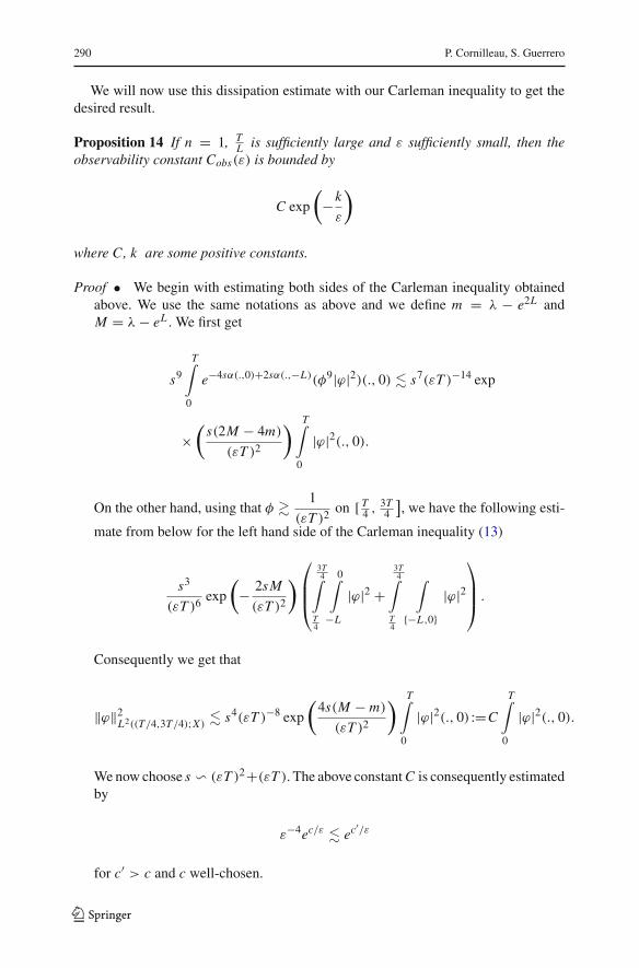
We will now use this dissipation estimate with our Carleman inequality to get thedesired result.
Proposition 14 If n = 1, TL is sufficiently large and ε sufficiently small, then the
observability constant Cobs(ε) is bounded by
C exp
(−k
ε
)
where C, k are some positive constants.
Proof • We begin with estimating both sides of the Carleman inequality obtainedabove. We use the same notations as above and we define m = λ − e2L andM = λ− eL . We first get
mate from below for the left hand side of the Carleman inequality (13)
s3
(εT )6exp
(− 2s M
(εT )2
)⎛⎜⎜⎝
3T4∫
T4
0∫−L
|ϕ|2 +3T4∫
T4
∫{−L ,0}
|ϕ|2⎞⎟⎟⎠ .
Consequently we get that
‖ϕ‖2L2((T/4,3T/4);X) � s4(εT )−8 exp
(4s(M − m)
(εT )2
) T∫0
|ϕ|2(., 0) :=C
T∫0
|ϕ|2(., 0).
We now choose s � (εT )2+(εT ). The above constant C is consequently estimatedby
ε−4ec/ε � ec′/ε
for c′ > c and c well-chosen.
123
Controllability and observability 291
• We now deduce the result using dissipation estimates. We have just proven
‖ϕ‖2L2((T/4,3T/4);X) � e
c′ε
T∫0
∫�0
|ϕ|2.
We now use the dissipation property with t1 = 0 and t2 = t ∈ ] T4 ,
3T4
[. We easily
get, provided T > 4L ,
T
2exp
((T − 4L)2
8εT
)‖ϕ(0)‖2
X � ‖ϕ‖2L2((T/4,3T/4);X),
which gives the result with k = 1
8
(1 − 4L
T
)(T − 4L)− c′ > 0 provided that
TL > 8 + 32c′. ��
3.2 Proof of Theorem 1
To show the controllability result for (Sv), we will adopt some minimization strategyinspired by the classical heat equation.
Proposition 15 A necessary and sufficient condition for the solution of problem (Sv)to satisfy u(T ) = 0 is given by:
∀ϕT ∈ X , 〈ϕ(0, .), u0〉X =T∫
0
ϕ(., 0)v.
where ϕ is the solution of problem (S′) with final value ϕT .
Proof We apply the Definition 4 to u against ϕ a strong solution of (S′), which gives
T∫0
ϕ(., 0)v = 〈ϕ(0, .), u0〉X − 〈ϕT , u(T, .)〉X
and we get the desired equivalence by approximation of weak solutions by strongsolutions. ��Proposition 16 The following properties are equivalent
• ∃C1 > 0,∀ϕT ∈ X; ‖ϕ(0, .)‖X ≤ C1‖ϕ(., 0)‖L2(0,T ) where ϕ is the solution ofproblem (S′),
• ∃C2 > 0,∀u0 ∈ X, ∃v ∈ L2(0, T ) such that ‖v‖L2(0,T ) � C2‖u0‖X and thesolution u of problem (Sv)satisfies u(T ) = 0.
Moreover, C1 = C2.
123
292 P. Cornilleau, S. Guerrero
Proof (⇒) Let u0 ∈ X . We define H as the closure of X for the norm defined by
‖ϕT ‖H = ‖ϕ(., 0)‖L2(0,T ),
where ϕ is the corresponding solution of (S′). Using the observability assumption andbackward uniqueness (Proposition 8), one sees that it is indeed a norm on X .
We define a functional J in the following way
J (ϕT ) = 1
2
T∫0
ϕ2(., 0)− 〈ϕ(0, .), u0〉X .
J is clearly convex and our assumption imply that J is continuous on H . Moreover,thanks to our observability assumption, J is coercive. Indeed, one has:
J (ϕT ) � 1
2‖ϕT ‖2
H − C‖ϕT ‖H
for ϕT ∈ H.Thus J possesses a global minimum ϕ̂T ∈ H , which gives, writing Euler–Lagrangeequations,
∀ϕT ∈ H,
T∫0
ϕ(., 0)ϕ̂(., 0) = 〈ϕ(0, .), u0〉X . (25)
According to Proposition 15, we have shown the existence of an admissible controldefined by v = ϕ̂(., 0). Moreover, choosing ϕT = ϕ̂T in (25), we obtain the followingestimate
‖v‖L2(0,T ) � ‖u0‖X‖ϕ̂(0, .)‖X .
Using our hypothesis, we are done.(⇐) If v is an admissible control with continuous dependence on u0, Proposition 15
gives us, for every ϕT ∈ X ,
〈ϕ(0, .), u0〈X=T∫
0
ϕ(., 0)v.
Choosing now u0 = ϕ(0) gives us the estimate
‖ϕ(0, .)‖2X � C2‖ϕT ‖H ‖u0‖X
123
Controllability and observability 293
that is
‖ϕ(0, .)‖X � C2‖ϕT ‖H .
��
4 Conclusion and open problems
The question of controllability in higher dimension is open and seems to be hard toobtain using Carleman estimates. Another approach to obtain the observability esti-mate in the n-dimensional case could be similar to the one of Miller (see [13, Theorem1.5]) but it seems that our problem is not adapted to that framework (we can check thatthe link between the one-dimensional problem and the general one is not as simple asit may seem, see Appendix A below).
If n = 1, we can wonder what is the minimal time to get a vanishing control costwhen the viscosity goes to zero. The intuitive result would be L , but it seems thatCarleman estimates cannot give such a result.
Appendix A: On Miller’s trick
In this paragraph, we detail why we cannot apply Miller’s method to deduce observ-ability in dimension n from the one in dimension 1. We refer the reader to the abstractsetting of [13, Section 2] (see more specifically Lemma 2.2 in that reference).
We denote by�1 or�n the domains (resp. X1 or Xn the function spaces, A1 or An
the evolution operators) in dimension 1 or n. The observability operator in dimensionone is defined by
O1 : ϕ −→ ϕ1{x=0}X1 → L2(∂�1)
.
where 1{x=0} is the characteristic function of {x = 0}.With similar notations, it is obvious that the observability operator on the part of
the boundary �0 = Rn−1 × {0} is given by
On : ϕ −→ ϕ1�0
Xn → L2(∂�n)
and coincides with the tensorial product I ⊗ O1 between the identity of L2(Rn−1)
and O1.We have now the following result.
Proposition 17 We define the natural “difference” between An and A1 by
B : w ∈ L2(Rn−1) → ε�′w ∈ L2(Rn−1)
123
294 P. Cornilleau, S. Guerrero
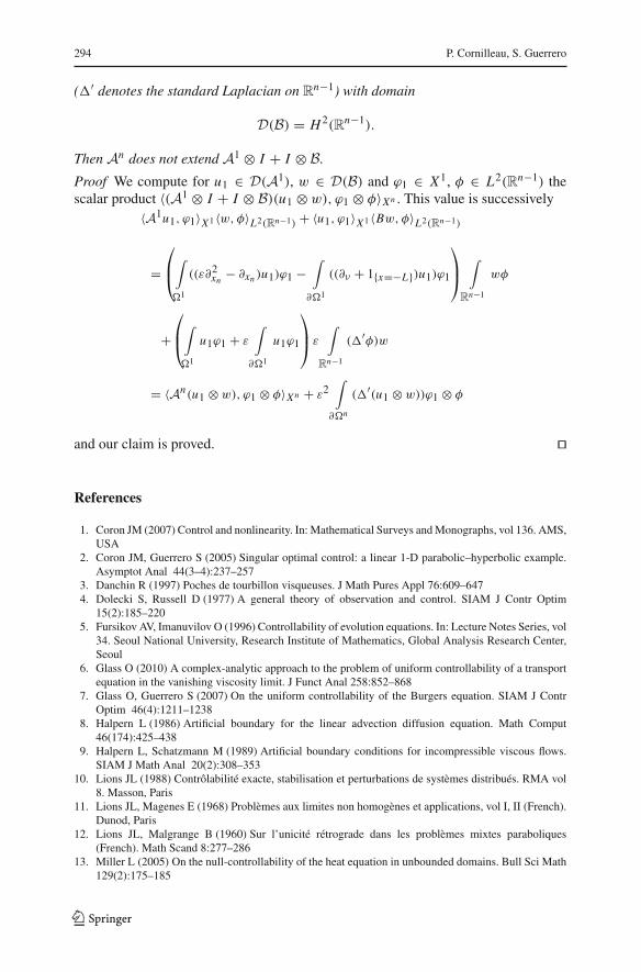
(�′ denotes the standard Laplacian on Rn−1) with domain
D(B) = H2(Rn−1).
Then An does not extend A1 ⊗ I + I ⊗ B.
Proof We compute for u1 ∈ D(A1), w ∈ D(B) and ϕ1 ∈ X1, φ ∈ L2(Rn−1) thescalar product 〈(A1 ⊗ I + I ⊗ B)(u1 ⊗ w), ϕ1 ⊗ φ〉Xn . This value is successively
1. Coron JM (2007) Control and nonlinearity. In: Mathematical Surveys and Monographs, vol 136. AMS,USA
2. Coron JM, Guerrero S (2005) Singular optimal control: a linear 1-D parabolic–hyperbolic example.Asymptot Anal 44(3–4):237–257
3. Danchin R (1997) Poches de tourbillon visqueuses. J Math Pures Appl 76:609–6474. Dolecki S, Russell D (1977) A general theory of observation and control. SIAM J Contr Optim
15(2):185–2205. Fursikov AV, Imanuvilov O (1996) Controllability of evolution equations. In: Lecture Notes Series, vol
34. Seoul National University, Research Institute of Mathematics, Global Analysis Research Center,Seoul
6. Glass O (2010) A complex-analytic approach to the problem of uniform controllability of a transportequation in the vanishing viscosity limit. J Funct Anal 258:852–868
7. Glass O, Guerrero S (2007) On the uniform controllability of the Burgers equation. SIAM J ContrOptim 46(4):1211–1238
8. Halpern L (1986) Artificial boundary for the linear advection diffusion equation. Math Comput46(174):425–438
9. Halpern L, Schatzmann M (1989) Artificial boundary conditions for incompressible viscous flows.SIAM J Math Anal 20(2):308–353
10. Lions JL (1988) Contrôlabilité exacte, stabilisation et perturbations de systèmes distribués. RMA vol8. Masson, Paris
11. Lions JL, Magenes E (1968) Problèmes aux limites non homogènes et applications, vol I, II (French).Dunod, Paris
12. Lions JL, Malgrange B (1960) Sur l’unicité rétrograde dans les problèmes mixtes paraboliques(French). Math Scand 8:277–286
13. Miller L (2005) On the null-controllability of the heat equation in unbounded domains. Bull Sci Math129(2):175–185