Controlled urban sprawl in Auckland, NewZealand and its impacts on the naturalenvironment and housing affordabilityTingting Xu1 and Jay Gao2*
Abstract
Auckland experienced phenomenal expansion since 1841. This study assesses the pace of urban sprawl and itscontrol over the natural environment and housing affordability. After the urban built-up area was mapped, itschange over time was detected, and correlated with population. From 1842 to 2014 built-up area in Auckland grewfrom 48 ha to 50,531 ha. The pace of growth was 151 ha/year during 1842–1945 but jumped to 989 ha per annumduring 1975–2001. It dropped to only 249 ha per annum in this century. This unchecked sprawl is a direct responseto population growth and facilitated by improved transportation. Since the late 1990s urban built-up areasexperienced a subdued expansion despite continued population growth. This curtailed sprawl is attributed to thecontentious planning regulations implemented to curtail sprawl. Consequently, population density rose to 28persons/ha, the highest since a century ago. Urban growth has reduced biomass and green fields with meanvegetation index dropped from 129.5 to 118.7 during 2002–2014 with a smaller standard deviation, suggesting thelandscape is increasingly homogenized. House prices rose slowly when the growth potential decreased slowly andvice versa (r = − 0.925) while the number of vacant sections suitable for single dwellings declined. Thus, controlledurban sprawl is largely responsible for the skyrocketed price of sections and declined housing affordability.
1 IntroductionUrban areas are the most important geographic zone tohuman beings and their socio-economic activities. Ac-cording to one estimate, approximately, 40% of theworld’s population, or around 3 billion people live inurban areas, and this percentage will increase in the fu-ture (UN-HABITAT, 2008). Unchecked urban growthwill lead to grave consequences, such as congestion, airquality deterioration, loss of amenity, and reduced bio-diversity and ecosystem service functions (Brody, 2013;Shao et al., 2021). In urban areas, a variety of uses arecompeting for precious land, including residential, com-mercial, industrial, recreational, and transport. The net
effect is the rapid urban sprawl that has encroachedupon the adjacent rural land. Urban sprawl refers to thenew development of urban areas (e.g., residential andshopping) in areas adjoining existing urban areas. Therapid expansion of urban areas requires periodic moni-toring to yield up-to-date information on urban landcovers and extent vital to urban planners. Such informa-tion can facilitate planning for future growth and avoid-ing costly planning mistakes. Timely and accuratemonitoring is also very important to understand the re-lationships and interactions between humans and thenatural environment (Feng & Li, 2012).Urban sprawl is most efficiently monitored using re-
mote sensing that can supply timely images current upto hours, which are especially valuable in monitoringareas of rapid urbanization and residential development.How to delineate the extent of suburban land cover
* Correspondence: [email protected] of Environment, University of Auckland, 23 Symonds Street,Auckland 1142, New ZealandFull list of author information is available at the end of the article
Computational UrbanScience
Xu and Gao Computational Urban Science (2021) 1:16 https://doi.org/10.1007/s43762-021-00017-8
using remote sensing caught the attention of remotesensing scientists as early as the beginning of this millen-nium (Epstein et al., 2002). In addition to Landsat multi-spectral scanner data (Yang & Lo, 2002), SPOT andSentinel data have been used for this purpose (Durieuxet al., 2008; Gao & Skillcorn, 1998; Jacquin et al., 2008;Phiri et al., 2020; Tong et al., 2010). The monitoringperiod can be extended further back if supplementedwith topographic maps and large-scale cadastral maps(Kurucu & Chiristina, 2008), and even aerial photo-graphs (Ma et al., 2008). Mapping of urban built-upareas is based primarily on impervious surfaces and theirspatial and temporal variability (Jat et al., 2008). Thegeneric workflow of monitoring urban growth fromtime-series satellite imagery involves change detection(Yang, 2011). One common method is the post-classification change detection technique through cross-tabulation (Shalaby et al., 2012). Urban sprawl can bemonitored by detecting changes in the mapped extent ofurban areas (Bhatta et al., 2010). Naturally, multi-temporal satellite data are ideal for this purpose (Feng &Li, 2012; Tang et al., 2006).The monitoring of urban sprawl is most effectively ac-
complished in GIS that is the best at storing and repro-ducing various kinds of integrated geospatial data(Kurucu & Chiristina, 2008). This integration is able toyield quantitative measurements needed for rapidlygrowing regions and in identifying the spatial variationsand temporal changes of urban sprawl patterns (Yeh &Li, 2001). The resulting information is presented visuallyin the form of urban-growth maps (Noda & Yamaguchi,2008). Remote sensing and GIS can be used to assess theimpacts of urban sprawl, such as the loss of cropland(Shalaby et al., 2012). The direct consequence of urbansprawl is the disappearance and fragmentation of forests(MacDonald & Rudel, 2005; Miller, 2012). After urbansprawl has been detected, it can be explained by its variousdrivers, such as population (Alsharif & Pradhan, 2014;Farooq & Ahmad, 2008). Land resource loss combinedwith population data allows a more nuanced interpret-ation of land-use change than in previous analyses ofurban sprawl (Hasse & Lathrop, 2003). In addition, the en-vironmental impact of urban sprawl has attracted muchattention in the literature. For instance, Martinuzzi et al.(2007) integrated census data with satellite imagery tostudy the human environment of urban sprawl in PuertoRico. Furberg and Ban (2012) assessed the potential envir-onmental impact of urban sprawl in the Greater Torontoarea. Nevertheless, this assessment focused on environ-mentally sensitive areas instead of the natural environ-ment in general, such as the loss of green fields. On theother hand, such information is indispensable for urbanplanners in designating new areas for constructing dwell-ings to cater to the needs of the additional population in
years to come. However, existing studies attempted to linkurban sprawl to population growth only within a time-frame of decades (Crankshaw & Borel-Saladin, 2019).Thus, the precise relationship between population andurban sprawl at different stages over a century or longerremains unexplored.In order to minimize the negative impacts of urban
sprawl such as traffic congestion and loss of biodiversity,some municipal governments around the world haveattempted to contain spiralling urban expansion throughzoning regulations. This attempt can curtail sprawl butcan have severe implications for living quality. In par-ticular, it may also provoke severe repercussions onhousing affordability as the regulations restrict the sup-ply of green fields for urban development. It is com-monly recognized that controlled urban sprawlnegatively impacts housing affordability. For instance, agreenbelt surrounding Seoul, South Korea prevented un-controlled urban sprawl and caused the real estate pricesin the inner city to soar (Dege, 2000), even though it ispossible to make more housing affordable and availablefor low-income households (Aurand, 2013). Althoughsprawl and the supply of affordable housing are posi-tively correlated for very low-income households inmetropolitan areas, there is no evidence to suggest thatcontrolled sprawl makes housing more affordable aftercontrolling for other metropolitan characteristics aretaken into account. On the other hand, significant urbansprawl in the Rocky Mountain region in the last decadeby the inward migration of population did cause real es-tate prices to spiral (Ghose, 2004). There exists a strongpositive relationship between restrictive land-use policiesand house prices (Gyourko, 2009). Thus, controlledurban sprawl has opposite effects on house prices in dif-ferent cities (e.g., leading to a higher price in some cities,but a lower price in other cities).The study has three objectives: (1) to determine the
rate and pattern of urban sprawling for Auckland fromits initial settlement by Europeans in the 1840s to thepresent; (2) to comparatively evaluate and explore thepace of growth in urban built-up extent in relation topopulation growth and government policy on urban landuse during the study period; (3) to assess the impact andimplications of curtailed urban sprawl in the city onpopulation density, the natural environment, and hous-ing affordability.
2 Study areaThe study site is the Auckland urban area located in theupper North Island of New Zealand (Fig. 1). AlthoughAuckland encompasses an administrative area of101,233 ha, its urban built-up area is much smaller at7489 ha (Rankin, 1979). The majority of it is confined toan isthmus between the Waitemata and Manukau
Xu and Gao Computational Urban Science (2021) 1:16 Page 2 of 12
Harbours, spreading outwards towards the surround-ing rural landscape in the north and the south. Thereis less population in the city’s eastern and westernareas where the landscape is dominated by mostlyrolling mountains. Auckland used to be inhabited bythe native people of Maori in the eighteenth centuryand was initially settled by Europeans since the early1840s. Abundant employment opportunities and themild weather saw the region’s population grow to 1.4million by 2013 (MacPherson, 2013), accountingroughly for one-third of the country’s total popula-tion. This population is projected to grow to 1.9 mil-lion by 2031 (Statistics NZ, 2010). The arrival ofmore people both domestically from the province andinternationally from other countries requires morehousing that is achieved via converting agriculturalland to residential use, which has contributed to
built-up area sprawl. Inevitably, it exerts some nega-tive impacts on the natural environment and increasesthe cost of servicing the newly urbanized areas. Thishas prompted the local government to enact planningstrategies to carefully manage such growth tominimize the impacts and to preserve living amenity.The efforts to contain urban growth have unexpectedconsequences on house affordability over the last dec-ade. This area of study was chosen because it has ex-perienced continuous urban sprawling since the citywas settled by the Europeans in the 1840s, and his-torical land cover maps dating back then were avail-able. Recently, the municipal government attemptedto contain urbanization mostly within its currenturban limit, which has caused housing prices to sky-rocket. This site serves as an excellent case to studyhow restrictive urban planning can affect the shape
Fig. 1 Administrative boundary of Auckland and its location in the North Island of New Zealand. Solid black line: metropolitan urban limit
Xu and Gao Computational Urban Science (2021) 1:16 Page 3 of 12
and pace of urban area development and its conse-quence on urban green fields and housingaffordability.
3 Methodology3.1 Data usedFour types of materials (data) were used in this study,historic town plan and land use maps, recent satelliteimages, census data, and real estate data. Historic townplan maps and recent land-use maps of Auckland werecollected from published sources and the Auckland Re-gional Council. These maps show the urban extent ofAuckland in nine years from 1842 to 2001. Additionalland cover maps were produced from two Landsat im-ages recorded on 18 April 2004 and 30 April 2014.More recent land covers were not analyzed due to thelack of land price data. Census data dating back from1842 to the present were acquired from Statistics NewZealand. Since census data are collected every 5 years,the year of census data does not always coincide with thetime of the land cover maps. The two can mismatch by amaximum of 2 years from each other. Real estate data of
2001–2014 are collected from the Real Estate Institute ofNew Zealand and Quotable Value New Zealand, the coun-try’s largest property information company.
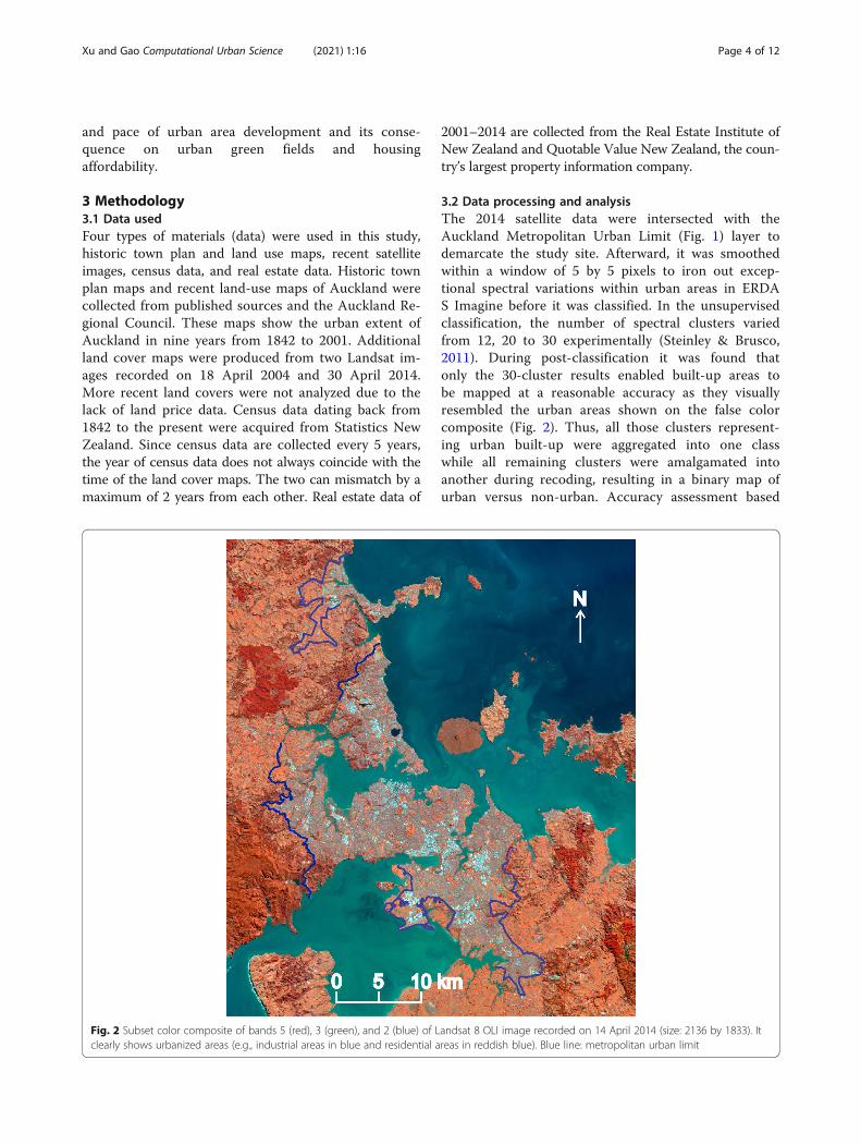
3.2 Data processing and analysisThe 2014 satellite data were intersected with theAuckland Metropolitan Urban Limit (Fig. 1) layer todemarcate the study site. Afterward, it was smoothedwithin a window of 5 by 5 pixels to iron out excep-tional spectral variations within urban areas in ERDAS Imagine before it was classified. In the unsupervisedclassification, the number of spectral clusters variedfrom 12, 20 to 30 experimentally (Steinley & Brusco,2011). During post-classification it was found thatonly the 30-cluster results enabled built-up areas tobe mapped at a reasonable accuracy as they visuallyresembled the urban areas shown on the false colorcomposite (Fig. 2). Thus, all those clusters represent-ing urban built-up were aggregated into one classwhile all remaining clusters were amalgamated intoanother during recoding, resulting in a binary map ofurban versus non-urban. Accuracy assessment based
Fig. 2 Subset color composite of bands 5 (red), 3 (green), and 2 (blue) of Landsat 8 OLI image recorded on 14 April 2014 (size: 2136 by 1833). Itclearly shows urbanized areas (e.g., industrial areas in blue and residential areas in reddish blue). Blue line: metropolitan urban limit
Xu and Gao Computational Urban Science (2021) 1:16 Page 4 of 12
on 60 evaluation pixels (30 urban built-up and 30non-urban pixels) revealed that the mapping of urbanareas was achieved at an accuracy higher than 95%owing to the large number of clusters specified be-forehand. Thus, the unsupervised classification resultswere deemed satisfactory and used subsequently todetect urban sprawl.During post-classification processing, the aggregated
and recoded results were spatially filtered usingclumping and sieving during which a threshold of 10pixels (an area of 0.9 ha on the ground) was specified.Any clusters with a membership < 10 pixels were re-moved from the output map. This filtered layer wastransformed into the vector format before beingexported to ArcGIS for further editing. Extensivemanual editing was undertaken to remove tiny spuri-ous polygons and to generalize boundaries of built-uppolygons. The edited vector layer was overlaid withother built-up layers of different years to illustrate thelocation of newly urbanized areas. The amount oftheir spatial extent was quantitatively determined inthe table environment.The mapped urban built-up area was statistically ana-
lyzed in relation to population in Excel to illustrate therelationship between the two. A similar analysis wasundertaken for house prices. The impact of urban sprawlon the natural environment was examined through nor-malized difference vegetation index (NDVI), an index in-dicative of the amount of biomass on the ground fromthe red (band 4) and near-infrared (band 5) bands ofLandsat 8 (bands 3 and 4 for Landsat 7). House pricedata were also correlated with the observed urban built-up area from satellite imagery.
4 Results4.1 Expansion of built-up areaThe initial settlement of Auckland in 1841 started fromthe landing at the waterfront near Britomart with mostof the administrative buildings clustered around thenearby streets in close proximity to each other in 1842(Fig. 3, left). Consequently, the built-up area was rathercompact at only 48 ha. Driven by inward immigration,the formerly disunited buildings had coalesced to formcontinuous, mostly residential blocks that had extendedwestwards by 1866. These settlements, not confined tothe southern shore of the Waitemata Harbor, totaled448 ha. Such a huge amount of built-up area representedan increase of nearly 15 fold at an annual rate of 17.7 ha.Five years later built-up area expanded by 249 ha toreach 697 ha. In addition to the former waterfront site,new and isolated settlements were founded in the distantsouth. During the Victoria-Edwardian era (1871–1915)the built-up area swelled 10 times larger to reach 5039ha due mostly to economic development. As the portcity for the hinterland, Auckland played a pivotal role inexporting goods produced in the country such as dairyproducts and timber (Bloomfield, 1967). The urbanizationrate was particularly high towards the late years of thisperiod. Consequently, nearly the entire northern half ofthe isthmus had been urbanized.This trend of rapid urban growth continued into the
two world war era between 1915 and 1945 during whichbuilt-up area nearly tripled to 13,642 ha at an annualrate of 287 ha. While the growth was spectacular in theisthmus itself, some areas in the north, east, and southwere also settled along the transport corridors. For in-stance, formerly isolated towns had been joined together
Fig. 3 The spatial extent of built-up areas in Auckland since the 1840s (Note: What is shown is the net expansion from the immediatelypreceding year to the current year. Thus, the urban built-up area in a later year encompasses that in all previous years). Note: The indicated yearswere selected because land cover maps were available for these years
Xu and Gao Computational Urban Science (2021) 1:16 Page 5 of 12
along the railway line. The built-up area nearly doubledto reach 26,793 ha at an annual rate of 692.16 ha duringthe post-war era of 1946 to 1964 (Fig. 3, middle).Growth was especially expansive in East Auckland, andto some degree, in the southwestern isthmus. Othernewly urbanized areas were confined to the west and thesouth along the trunk roads and adjoining formerly set-tled areas. The advent of private cars and improvedroads and public transport enabled suburbs much fur-ther from waterfront Auckland to be urbanized. Statehousing for the war veterans, together with factoriesspurred by the provision of electricity, was responsiblelargely for the expansion of built-up areas in East Auck-land. This vast pace of growth was also a direct responseto expanded manufacturing that created employment forthousands of new arrivals who further fueled suburbanexpansion (Bloomfield, 1967). During the next decade(1964–1975), the built-up area of Auckland continuedits accelerated growth to reach 37,000 ha at an annualrate of 927.91 ha. As shown in Fig. 3 (right), most of thenewly urbanized areas are confined to the south, thewest, and the north owing to the improved transport in-frastructure such as motorways. They opened up newareas for settlement. In addition, coastal areas like theeast and far north had been developed, mostly for resi-dential use due to the naturally appealing landscape.This pattern of growth is attributed mostly to the open-ing of the harbor bridge in 1953.In contrast to the spectacular growth over the previous
period of 1975–2001, the pace of growth during 2001–2014 is subdued. The majority of the new growth was
confined to East and South Auckland that used to be ex-tensive and expansive flat green fields suitable for con-version to residential dwellings. The urban area rosemarginally to only 49,520 ha by 2008 and 50,531 ha by2014. Most of the newly urbanized areas during this cen-tury were situated in the north and south, all being smallin size (Fig. 4, right). The expansion in the north shorefurther away from the coast and the northwest was re-lated to the construction of the second bridge in theupper harbor. The rate of growth decreased from 989 haper annum during 1975–2001 to only 249 ha per annumduring 2001–2014. By 2014 the built-up area expandedby less than 200 ha per annum. Most of the newly ur-banized areas are located in the south and the north ofthe city, nearly all of them from market gardens and pas-ture. They are rather small in their spatial extent, all ad-joining existing built-up areas unexceptionally. Thus, thepace of expansion has slowed down to a fraction of thatof decades earlier. Apparently, the unbridled urbansprawl of Auckland over the previous periods has beenbrought under control by this stage.
4.2 Built-up area vs populationFigure 4 illustrates the relationship between urban built-up area and population growth during 1842–2014. Over-all, the two variables are highly correlated with eachother (R2 = 0.944). The growth pattern falls into threeperiods of undergrowth, unchecked growth, and curtailedgrowth. The first period took place in the nineteenth cen-tury when the population grew at a faster pace than built-up area expansion. There was no sprawl at all. During the
Fig. 4 Relationship between urban built-up area and population between 1842 and 2014. Note: (1) Not all the populations dwelled within theAuckland metropolitan urban limit due to changed administrative boundaries over the years; and (2) Population data and the urban built-up areamay not be obtained in the same year because census took place every five years. Only the census data closest to the land cover map in timewere used
Xu and Gao Computational Urban Science (2021) 1:16 Page 6 of 12
second period that covered the first 90 years of the twenti-eth century, both population and the urban built-up areagrew slowly but steadily at an almost identical pace until1945. Afterward, they underwent a steep rise until reach-ing a plateau in 1975 when both stagnated slightly follow-ing the stock market crash in 1989. The two have beengrowing at an almost identical rate with a high correlationbetween them until the 1990s. Employment opportunitiesand migration have seen a rapid rise in the city’s popula-tion over the last two decades that has been accommo-dated via the ever-expanding built-up areas. According tothis diagram, the 1000-fold expansion of the urban built-up area is a direct response to explosive populationgrowth. However, entering the third period, the twotrends of growth started to diverge from the 1990s whenplanning regulations imposed a limit on urban sprawl soas to control run-away infrastructure costs. On the onehand, the population continued to rise steeply while built-up areas rose marginally in comparison, resulting in a gen-tly inclined curve. As clearly shown in the diagram, the ef-fort to curtail urban sprawl is rather successful. However,this containment is achieved at the expense of reduced liv-ing amenity (e.g., a much higher population density) andsocial cost in that real estate price has skyrocketed beyondthe affordability of many residents.The direct impact of the curtailed sprawl is a general
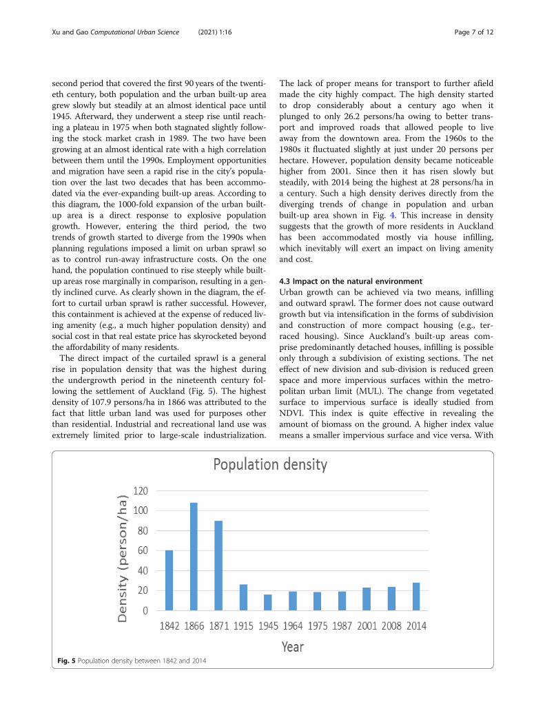
rise in population density that was the highest duringthe undergrowth period in the nineteenth century fol-lowing the settlement of Auckland (Fig. 5). The highestdensity of 107.9 persons/ha in 1866 was attributed to thefact that little urban land was used for purposes otherthan residential. Industrial and recreational land use wasextremely limited prior to large-scale industrialization.
The lack of proper means for transport to further afieldmade the city highly compact. The high density startedto drop considerably about a century ago when itplunged to only 26.2 persons/ha owing to better trans-port and improved roads that allowed people to liveaway from the downtown area. From the 1960s to the1980s it fluctuated slightly at just under 20 persons perhectare. However, population density became noticeablehigher from 2001. Since then it has risen slowly butsteadily, with 2014 being the highest at 28 persons/ha ina century. Such a high density derives directly from thediverging trends of change in population and urbanbuilt-up area shown in Fig. 4. This increase in densitysuggests that the growth of more residents in Aucklandhas been accommodated mostly via house infilling,which inevitably will exert an impact on living amenityand cost.
4.3 Impact on the natural environmentUrban growth can be achieved via two means, infillingand outward sprawl. The former does not cause outwardgrowth but via intensification in the forms of subdivisionand construction of more compact housing (e.g., ter-raced housing). Since Auckland’s built-up areas com-prise predominantly detached houses, infilling is possibleonly through a subdivision of existing sections. The neteffect of new division and sub-division is reduced greenspace and more impervious surfaces within the metro-politan urban limit (MUL). The change from vegetatedsurface to impervious surface is ideally studied fromNDVI. This index is quite effective in revealing theamount of biomass on the ground. A higher index valuemeans a smaller impervious surface and vice versa. With
Fig. 5 Population density between 1842 and 2014
Xu and Gao Computational Urban Science (2021) 1:16 Page 7 of 12
the intensification of housing, fewer green fields are leftwithin the current urban limit, and hence a lower NDVIvalue.Figure 6 visualizes the spatial distribution of NDVI
values in 2004 and 2014. The two results are obtainedwithin only 12 Julian days from each other, so the differ-ence in NDVI between the two results caused by naturalvariability is reduced to a minimum. Overall, the meanNDVI value decreased from 129.5 in 2004 to 118.7 in2014. Besides, the standard deviation of NDVI valueshas almost halved from 17.21 to 9.28, meaning that thelandscape is becoming increasingly homogenized in itsland covers (e.g., covered by concrete surfaces). The de-crease in NDVI value is rather obvious at certain spots.The most noticeable is Flatbush (A) in the southeast.The former spatially expansive green area has drasticallyshrunk in its extent. Another noticeable area of changetook place in Orewa (B) in the north. The former greenarea has become more fragmented with a lower NDVIvalue. The land has been converted mostly to residentialuses with a moderate NDVI value, but also increasinglyred (industrial and terraced housing with little greenspace between houses). The third area of considerabledecrease in green fields is Henderson Creek in the west(C). Although some green fields remain, their area hasshrunk with the remaining green fields more fragmen-ted. These kinds of changes at the urban fringe tookplace in the form of conversion from green fields tourban uses on a wholescale scale. In addition, changes inthe form of subdivisions also took place. It also reducedNDVI values, although not as significant as the new
division. Since the two NDVI maps do not have thesame legend, the change in NDVI caused by house infillin the form of subdivision within built-up areas is verydifficult to appreciate in Fig. 6.
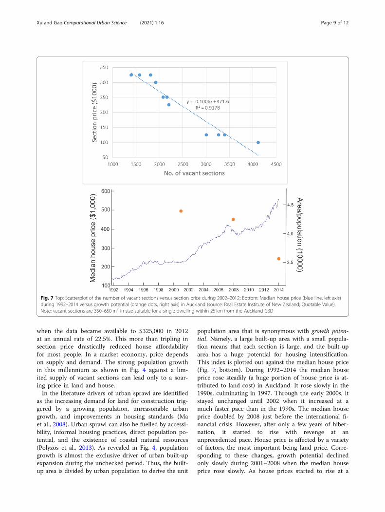
4.4 Built-up area vs housing affordabilityOne prerequisite of urban sprawl is the conversion ofrural uses such as market gardens and pasture intourban use in which the land must be divided into sec-tions for dwelling construction, the most direct way ofgauging the impact of controlled sprawl is to examinethe availability of sections for sale. Shown in Fig. 7a isthe dwindled supply of 350–650 m2 vacant sections suit-able for a single dwelling in established urban areaswithin a radius of 25 km from Auckland’s central busi-ness district. It experienced a steady decrease from 4116in 2002 to only 1402 in 2012, a decrease of 65.9%(source: Quotable Value). On average, the number of va-cant sections decreased by 10% annually over the dec-ade. In other words, most of the land earmarked forurban development had been depleted quickly over thepreceding unchecked period of sprawl. The dwindlingsupply of smaller sections than in the previous decadesand/or the controlled release of more green fields forhousing have contributed to the slowdown sprawling.In sharp contrast to this decline is the steady increasein the price of vacant sections during the same period(Fig. 7, top). The two are correlated inversely witheach other, with 91.78% of the variations in sectionprice (R2) accounted for by the number of vacant sec-tions. Section price rose from NZ$100,000 from 2002
Fig. 6 Comparison of the spatial variation in NDVI for the city of Auckland. (a) 18 April 2004 (mean NDVI = 129.5; Standard deviation = 17.21); (b)30 April 2014 (mean NDVI = 118.7; standard deviation = 9.28). Note: Some areas experienced a higher NDVI value due to the natural growthof vegetation
Xu and Gao Computational Urban Science (2021) 1:16 Page 8 of 12
when the data became available to $325,000 in 2012at an annual rate of 22.5%. This more than tripling insection price drastically reduced house affordabilityfor most people. In a market economy, price dependson supply and demand. The strong population growthin this millennium as shown in Fig. 4 against a lim-ited supply of vacant sections can lead only to a soar-ing price in land and house.In the literature drivers of urban sprawl are identified
as the increasing demand for land for construction trig-gered by a growing population, unreasonable urbangrowth, and improvements in housing standards (Maet al., 2008). Urban sprawl can also be fuelled by accessi-bility, informal housing practices, direct population po-tential, and the existence of coastal natural resources(Polyzos et al., 2013). As revealed in Fig. 4, populationgrowth is almost the exclusive driver of urban built-upexpansion during the unchecked period. Thus, the built-up area is divided by urban population to derive the unit
population area that is synonymous with growth poten-tial. Namely, a large built-up area with a small popula-tion means that each section is large, and the built-uparea has a huge potential for housing intensification.This index is plotted out against the median house price(Fig. 7, bottom). During 1992–2014 the median houseprice rose steadily (a huge portion of house price is at-tributed to land cost) in Auckland. It rose slowly in the1990s, culminating in 1997. Through the early 2000s, itstayed unchanged until 2002 when it increased at amuch faster pace than in the 1990s. The median houseprice doubled by 2008 just before the international fi-nancial crisis. However, after only a few years of hiber-nation, it started to rise with revenge at anunprecedented pace. House price is affected by a varietyof factors, the most important being land price. Corre-sponding to these changes, growth potential declinedonly slowly during 2001–2008 when the median houseprice rose slowly. As house prices started to rise at a
Fig. 7 Top: Scatterplot of the number of vacant sections versus section price during 2002–2012; Bottom: Median house price (blue line, left axis)during 1992–2014 versus growth potential (orange dots, right axis) in Auckland (source: Real Estate Institute of New Zealand; Quotable Value).Note: vacant sections are 350–650m2 in size suitable for a single dwelling within 25 km from the Auckland CBD
Xu and Gao Computational Urban Science (2021) 1:16 Page 9 of 12
faster pace, the decline in the growth potential also ac-celerated. The period of the fastest house price rise cor-responds to a period of the steepest decline in growthpotential (Fig. 7, bottom). Due to the small number ofobservations available, it is impossible to establish aquantitative regression relationship between the two.The correlation coefficient based on the three availableobservations is as high as − 0.925, remarkably similar tobut slightly lower than that (− 0.958) between the num-ber of available vacant sections and section price. There-fore, the policy of maintaining urban growth within theexisting urban limit is the main culprit of the sky-rocketed housing price and abysmal housingunaffordability.
5 DiscussionThe subdued increment in built-up areas in this century(Fig. 3) differs sharply from the fast rise in the precedingperiod, even though Auckland’s population maintainedthe same pace of growth. The divergence of the two to-wards the later 1990s results from both land depletionand planning policies. In the literature, the role of crit-ical policies in affecting urban sprawl has been noted(Yue et al., 2013). Auckland is no exception. Aucklandhousing used to be dominated by standalone dwellingsconstructed over a ‘quarter acre’ (1000 m2) section in anera when the population was small and residential landbountiful. This generous land use practice was drivingthe unstoppable urban sprawl in the first 80 years of thetwentieth century. Such unchecked sprawl overburdensestablishing new and maintaining ever more infrastruc-ture. In addition, it imposes a heavy toll on the govern-ment to provide services, such as bus, utility, and stormwater treatment. More sprawl means more skyrocketedcosts in providing such services in sparsely populatedareas. Apparently, such an inefficient allocation of landresources for urban use is not sustainable in light of in-ternal migration and inbound international immigrationassociated with globalization. This prompted the localauthorities to promulgate planning regulations to limiturban sprawl so as to control run-away infrastructurecosts. The policy is commonly known as MetropolitanUrban Limit that has been in existence for over half acentury. This legal document sets out the rules for urbandevelopment and subdivisions to reduce runaway infra-structural costs. This zoning boundary demarcates theurban area within which urban development is allowed(Auckland Regional Growth Forum, 1999). It still exertsan impact even today as “over the next 30 years for280,000 new dwellings within the 2010 MetropolitanUrban Limit baseline, 160,000 will be built in new greenfields land, satellite towns, and other rural and coastaltowns” (Auckland Council, 2012). Consequently, theland inside the MUL is around 10 times more expensive
than land just outside it (Grimes & Liang, 2009). The at-tempt to confine new growth mostly within the existingurban limit is directly responsible for the divergence ofthe two trends of growth from the 1990s onwards.Therefore, the MUL is a binding and increasing con-straint on land supply at a time when housing demandhas intensified (Zheng, 2013).The desire to build a compact city with minimal im-
pacts on the natural environment has some unexpectedconsequences on housing affordability. This issue can bebetter addressed by modifying other planning policiescommensurately to accommodate the continuous influxof migrants. For instance, the minimum section size canbe reduced to allow housing intensification and the re-striction on building height can be relaxed to allowhigh-rise housing development to dent the section price.To strike a delicate balance between building a compactcity and maintaining affordable housing, certain restric-tions on urban development must be relaxed in light ofcontinuous inward migration, even though these changesmay degrade the amenity of existing urban areas.Elsewhere rapid urbanization has been associated with
the construction of infrastructures such as airports andhighways in developing countries (Pourebrahim et al.,2015). Auckland is no exception. Certainly, the consider-able expansion of Auckland towards the southeast andthe north (Northshore) in the 1960s and 1970s (Fig. 3)can be attributed to the completion of Auckland SouthernMotorway in 1953 and the opening of the AucklandHarbour Bridge in 1959, respectively. It must be empha-sized, nevertheless, infrastructure is critical to shaping theurbanized area, but it may not affect the total amount ofurbanized areas critically.
6 ConclusionsSince its initial settlement by Europeans in 1842,Auckland has sprawled by 1000 folds in its built-uparea to reach 50,531 ha in 2014 at an uneven pace ofgrowth during different periods. Settled areas weresmall and compact in the nineteenth century owingto the lack of transport and not-so-developed econ-omy. With the development in economic activitiesand the arrival of migrants from rural areas, theurban area expanded steadily in the early twentiethcentury, an outcome facilitated by better transport in-frastructure. Auckland experienced explosive growthbetween the two world wars during which the built-up area nearly tripled. Urban sprawl culminated toreach an annual rate of nearly 1000 ha in the 1960sand 1970s when there was an unlimited supply ofmostly flat agricultural land. The spectacular expan-sion in built-up areas was facilitated by improvementsin transport infrastructure, including railways, motor-ways, and bridges. Both population and urban built-
Xu and Gao Computational Urban Science (2021) 1:16 Page 10 of 12
up areas grew at the same pace until the late 1990swhen growth in built-up areas was curtailed despitethe continued population growth driven partially byimmigration. It grew by only 3235 ha to reach 50,531ha during 2001–2014 at a rate of 249 ha per annum,only a quarter of the rate in the preceding period.This urban growth has negatively impacted the livingenvironment in that the NDVI, an indicator of bio-mass on the ground, declined from 129.5 in 2004 to118.7 10 years later while its standard deviation be-came smaller as well. This indicated that the land-scape is increasingly homogenized with former greenfields converted to urban uses in peri-urban areas.The curtailed sprawl in this century is accounted forby the contentious planning regulation designed tocontain urban growth to mostly within the existingMetropolitan Urban Limit. This regulation has causedhousing increasingly unaffordable as judged by thedwindling number of vacant sections suitable for sin-gle dwellings. It bears a close correlation with sectionprice at r = − 0.958. The increase in the median houseprice experienced an exactly opposite change to thatin growth potential (r = − 0.925). The fact that thegrowth potential decreased slowly when house pricesrose only slowly but dropped substantially when themedian house price skyrocketed suggests that the ef-fort in containing urban sprawl through legislativeboundary is the primary culprit of house unaffordabil-ity. More observations are needed to quantify theexact contribution of curtailed sprawl on house pricerise.
Code availabilityNo applicable.
Authors’ contributionsTingting Xu: 70% (did most of the data analysis); Jay Gao: 30% (wrotethe manuscript and drew the illustrations).
FundingThis research was supported by an internal research grant from theUniversity of Auckland.
Availability of data and materialsThe data are satellite images available from Google Earth Engine.
Declarations
Competing interestsNo conflicts of interest.
Author details1School of Software Engineering, Chongqing University of Posts andTelecommunications, No.2 Chongwen Road, Nanshan, Chongqing 400000,China. 2School of Environment, University of Auckland, 23 Symonds Street,Auckland 1142, New Zealand.
Received: 24 May 2021 Accepted: 12 July 2021
ReferencesAlsharif, A. A. A., & Pradhan, B. (2014). Urban sprawl analysis of Tripoli
Metropolitan City (Libya) using remote sensing data and multivariate logisticregression model. Journal Indian Society Remote Sensing, 42(1), 149–163.https://doi.org/10.1007/s12524-013-0299-7.
Auckland Council (2012). The Auckland plan - a plan for all Aucklanders. aucklandcouncil.govt.nz
Aurand, A. (2013). Does sprawl induce affordable housing? Growth Change, 44(4),631–649. https://doi.org/10.1111/grow.12024.
Bhatta, B., Saraswati, S., & Bandyopadhyay, D. (2010). Quantifying the degree-of-freedom, degree-of-sprawl, and degree-of-goodness of urban growth fromremote sensing data. Applied Geography, 30(1), 96–111. https://doi.org/10.1016/j.apgeog.2009.08.001.
Bloomfield, G. T. (1967). The growth of Auckland. In J. S. Whitelaw (Ed.), Aucklandin Ferment (pp. 1–12). New Zealand Geographical Society.
Brody, S. (2013). The characteristics, causes, and consequences of sprawlingdevelopment patterns in the United States. Nature Education Knowledge, 4(5),2 https://www.nature.com/scitable/knowledge/library/the-characteristics-causes-and-consequences-of-sprawling-103014747/.
Crankshaw, O., & Borel-Saladin, J. (2019). Causes of urbanisation and counter-urbanisation in Zambia: Natural population increase or migration? UrbanStudies, 56(10), 2005–2020. https://doi.org/10.1177/0042098018787964.
Dege, E. (2000). Seoul: From capital to capital region. Geographische Rundschau,52(7–8), 4–10 (in German).
Durieux, L., Lagabrielle, E., & Nelson, A. (2008). A method for monitoring buildingconstruction in urban sprawl areas using object-based analysis of Spot 5images and existing GIS data. ISPRS Journal Photogrammetry Remote Sensing,63(4), 399–408. https://doi.org/10.1016/j.isprsjprs.2008.01.005.
Epstein, J., Payne, K., & Kramer, E. (2002). Techniques for mapping suburbansprawl. Photogrammetric Engineering Remote Sensing, 68(9), 913–918.
Farooq, S., & Ahmad, S. (2008). Urban sprawl development around Aligarh city: Astudy aided by satellite remote sensing and GIS. Journal Indian SocietyRemote Sensing, 36(1), 77–88. https://doi.org/10.1007/s12524-008-0008-0.
Feng, L., & Li, H. (2012). Spatial pattern analysis of urban sprawl: Case study ofJiangning, Nanjing, China. Journal Urban Planning Development, 138(3), 263–269. https://doi.org/10.1061/(ASCE)UP.1943-5444.0000119.
Furberg, D., & Ban, Y. (2012). Satellite monitoring of urban sprawl and assessmentof its potential environmental impact in the greater Toronto area between1985 and 2005. Environmental Management, 50(6), 1068–1088. https://doi.org/10.1007/s00267-012-9944-0.
Gao, J., & Skillcorn, D. (1998). Capability of SPOT XS data in producing detailedland cover maps at the urban–rural periphery. International Journal RemoteSensing, 19(15), 2877–2891. https://doi.org/10.1080/014311698214325.
Ghose, R. (2004). Big sky or big sprawl? Rural gentrification and the changingcultural landscape of Missoula, Montana. Urban Geography, 25(6), 528–549.https://doi.org/10.2747/0272-3638.25.6.528.
Grimes, A., & Liang, Y. (2009). Spatial determinants of land prices in Auckland:Does the metropolitan urban limit have an effect? Applied Spatial AnalysisPolicy, 2(1), 23–45. https://doi.org/10.1007/s12061-008-9010-8.
Gyourko, J. (2009). Housing supply. Annual Review Economics, 1(1), 295–318.https://doi.org/10.1146/annurev.economics.050708.142907.
Hasse, J. E., & Lathrop, R. G. (2003). Land resource impact indicators of urbansprawl. Applied Geography, 23(2–3), 159–175. https://doi.org/10.1016/j.apgeog.2003.08.002.
Jacquin, A., Misakova, L., & Gay, M. (2008). A hybrid object-based classificationapproach for mapping urban sprawl in peri-urban environment. LandscapeUrban Planning, 84(2), 152–165. https://doi.org/10.1016/j.landurbplan.2007.07.006.
Jat, M. K., Garg, P. K., & Khare, D. (2008). Monitoring and modelling of urbansprawl using remote sensing and GIS techniques. International JournalApplied Earth Observation Geoinformation, 10(1), 26–43. https://doi.org/10.1016/j.jag.2007.04.002.
Kurucu, Y., & Chiristina, N. K. (2008). Monitoring the impacts of urbanization andindustrialization on the agricultural land and environment of the Torbali,Izmir region, Turkey. Environmental Monitoring Assessment, 136(1–3), 289–297.https://doi.org/10.1007/s10661-007-9684-4.
Xu and Gao Computational Urban Science (2021) 1:16 Page 11 of 12
Ma, M., Lu, Z., & Sun, Y. (2008). Population growth, urban sprawl and landscapeintegrity of Beijing City. International Journal Sustainable Development WorldEcology, 15(4), 326–330. https://doi.org/10.3843/SusDev.15.4:6.
MacDonald, K., & Rudel, T. K. (2005). Sprawl and forest cover: What is therelationship? Applied Geography, 25(1), 67–79. https://doi.org/10.1016/j.apgeog.2004.07.001.
MacPherson, L. (2013). 2013 census usually resident population counts (p. 18).Statistics NZ.
Martinuzzi, S., Gould, W. A., & Ramos González, O. M. (2007). Land development,land use, and urban sprawl in Puerto Rico integrating remote sensing andpopulation census data. Landscape Urban Planning, 79(3–4), 288–297. https://doi.org/10.1016/j.landurbplan.2006.02.014.
Miller, M. D. (2012). The impacts of Atlanta’s urban sprawl on forest cover andfragmentation. Applied Geography, 34, 171–179. https://doi.org/10.1016/j.apgeog.2011.11.010.
Noda, A., & Yamaguchi, Y. (2008). Characterizing urban sprawl using remotesensing and a simple spatial metric for a medium-sized city in Japan.International Journal Geoinformatics, 4(1), 43–50.
Phiri, D., Simwanda, M., Salekin, S., Nyirenda, V. R., Murayama, Y., & Ranagalage, M.(2020). Sentinel-2 data for land cover/use mapping: A review. RemoteSensing, 12(14), 2291. https://doi.org/10.3390/rs12142291.
Polyzos, S., Minetos, D., & Niavis, S. (2013). Driving factors and empirical analysisof urban sprawl in Greece. Theoretical Empirical Researches UrbanManagement, 8(1), 5–29.
Pourebrahim, S., Hadipour, M., & Mokhtar, M. B. (2015). Impact assessment ofrapid development on land use change in coastal areas: Case of KualaLangat district, Malaysia. Environment Development and Sustainability, 17,1003–1016. https://doi.org/10.1007/s10668-014-9585-y.
Rankin, D. G. (1979). Urban Auckland. In W. Moran & M. J. Taylor (Eds.), Aucklandand the central North Island (pp. 88–113). Longman Paul.
Shalaby, A. A., Ali, R. R., & Gad, A. (2012). Urban sprawl impact assessment on theagricultural land in Egypt using remote sensing and GIS: A case study,Qalubiya governorate. Journal Land Use Science, 7(3), 261–273. https://doi.org/10.1080/1747423X.2011.562928.
Shao, Z., Sumari, N. S., Portnov, A., Ujoh, F., Musakwa, W., & Mandela, P. J. (2021).Urban sprawl and its impact on sustainable urban development: Acombination of remote sensing and social media data. Geo SpatialInformation Science, 24(2), 241–255. https://doi.org/10.1080/10095020.2020.1787800.
Statistics NZ, 2010. Mapping Trends in the Auckland Region, Retrieved 23 July2014, from http://www.stats.govt.nz/browse_for_stats/people_and_communities/Geographic-areas/mapping-trends-in-the-auckland-region/population-change.aspx#.
Steinley, D., & Brusco, M. (2011). Choosing the number of clusters in K-meansclustering. Psychological Methods, 16(3), 285–297. https://doi.org/10.1037/a0023346.
Tong, X., Zhang, X., & Liu, M. (2010). Detection of urban sprawl using a geneticalgorithm-evolved artificial neural network classification in remote sensing: Acase study in Jiading and Putuo districts of Shanghai, China. InternationalJournal Remote Sensing, 31(6), 1485–1504. https://doi.org/10.1080/01431160903475290.
UN-HABITAT. (2008). State of the World’s cities 2010/2011 - bridging the urbandivide (p. 244). Earthscan.
Yang, Y. (2011). Use of archival Landsat imagery to monitor urban spatial growth.In X. Yang (Ed.), Urban remote Sensing: Monitoring, Synthesis and Modeling inthe Urban Environment. Wiley. https://doi.org/10.1002/9780470979563.ch2.
Yang, Y., & Lo, C. P. (2002). Using a time series of satellite imagery to detect landuse and land cover changes in the Atlanta, Georgia metropolitan area.International Journal Remote Sensing, 23(9), 1775–1798. https://doi.org/10.1080/01431160110075802.
Yeh, A. G.-O., & Li, X. (2001). Measurement and monitoring of urban sprawl in arapidly growing region using entropy. Photogrammetric Engineering RemoteSensing, 67(1), 83–90.
Yue, W., Liu, Y., & Fan, P. (2013). Measuring urban sprawl and its drivers in largeChinese cities: The case of Hangzhou. Land Use Policy, 31, 358–370. https://doi.org/10.1016/j.landusepol.2012.07.018.
Zheng, Y. (2013). The effect of Auckland’s metropolitan urban limit on landprices. In The New Zealand Productivity Commission (p. 18).
Publisher’s NoteSpringer Nature remains neutral with regard to jurisdictional claims inpublished maps and institutional affiliations.
Xu and Gao Computational Urban Science (2021) 1:16 Page 12 of 12