Int. J. Advance. Soft Comput. Appl., Vol. 4, No. 2, July 2012
ISSN 2074-8523; Copyright © ICSRS Publication, 2012
www.i-csrs.org
CONTROLLER TUNING FOR INDUSTRIAL
PROCESS-A SOFT COMPUTING
APPROACH
B.Nagaraj,P.Vijayakumar
Corresponding author, Karunya University, Coimbatore, India
email:[email protected]
Karapagam College of Engineering, Coimbatore, India
Abstract
Proportional – Integral – Derivative control schemes continue to provide
the simplest and effective solutions to most of the control engineering
applications today. However PID controller is poorly tuned in practice with most
of the tuning done manually which is difficult and time consuming. This research
comes up with a soft computing approach involving Genetic Algorithm,
Evolutionary Programming, Particle Swarm Optimization and Bacterial foraging
optimization. The proposed algorithm is used to tune the PI parameters and its
performance has been compared with the conventional methods like Ziegler
Nichols and Cohen Coon method. The results obtained reflect that use of
heuristic algorithm based controller improves the performance of process in
terms of time domain specifications, set point tracking and regulatory changes
and also provides an optimum stability. This paper discusses in detail, the Soft
computing technique and its implementation in PI tuning for a controller of a
real time process. Compared to other conventional PI tuning methods, the result
shows that better performance can be achieved with the soft computing based
tuning method. The ability of the designed controller in terms, of tracking set
point is also compared and simulation results are shown.
Keywords: Bacterial foraging, Genetic algorithm, Particle swarm optimization,
PID controller
1 Introduction
PID controller is a generic control loop feedback mechanism widely used in
industrial control systems [1]. It calculates an error value as the difference between
measured process variable and a desired set point [2]. The PID controller
calculation involves three separate parameters proportional, integral and derivative
values. The goal of PID controller tuning is to determine parameters that meet
closed loop system performance specifications and the robust performance of the
control loop over a wide range of operating conditions should also be ensured.
Practically, it is often difficult to simultaneously achieve all of these desirable
qualities [3]. The purpose of this paper is to investigate an optimal controller design
for a simple process in Paper machine using the evolutionary Programming, Genetic
Algorithm, Particle Swarm Optimization and Bacterial foraging Optimization.
Objective of the research is to develop a soft computing based PID tuning
methodology for optimizing the control of a simple Process plant that is housed in
the Paper Machine#3 at the Tamilnadu Newsprint and Papers Limited, India. The
main variables under control are chemical flow, Pump discharge pressure and tank
level. This research proposes the development of a tuning technique that would be
best suitable for optimizing the processes operating in a single-input-single-output
(SISO) process control loop. The SISO topology has been selected for this study
because it is the most fundamental of control loops and the theory developed for
this type of loop can be easily extended to more complex loops [4]. The efficacy of
the proposed method has been proved to be the best by comparing the control
performance of loops with the soft computing method to that of loops tuned using
the conventional method of Ziegler-Nichols method.
2 Development of a Mathematical model of Real Time
Process
The plant used for this study is given in appendix (fig.9) and its corresponding P &
ID schematic is shown in Fig 1. The plant consists of a storage tank: Process tank
feed chemical pump, Control Valve and Pressure level and flow transmitters. A
feed-pump supplies chemical from the storage tank to the process tank. The
Pressure transmitter (PT 0.01A), which is situated downstream of the pump,
provides an indication of pump discharge pressure and volume of water moved by
the pump. Control valve (CV 0.01A) is situated between the flow transmitter and
the process tank to manipulate the flow and thus control the discharge pressure and
the level of water in the process tank. Control of the water flow rate (FT 0.01A),
line pressure (PT 0.01A) and process tank level (LT0.01A) is achieved separately
using the control valve (CV 0.01A) during each control session. A current to
pressure (I/P) converter is used to provide correct signal interface to the control
valve (CV 0.01A), which operates from a 4 bar air supply.
Fig.1. P&ID of the plant under study.
2.1 Identification of Process Parameters
The Process model used in the experiments for the pressure, flow and level control
loops are given in (1), (2) and (3) respectively. Models (1)-(3) were identified with
Matlab system identification tool box[5] and used to determine the tuning
parameters by means of the ZN, GA, EP, PSO and BFO tuning methodologies.
Pressure Control System:
--------- (1)
Flow Control System:
15.3224.1
5.6exp5.0
SS
SsflowGP
-------- (2)
Level Control System:
--------- (3)
3 Design of PID Controller
After deriving the transfer function model the controller has to be designed for
maintaining the system to the optimal set point. This can be achieved by properly
selecting the tuning parameters Kp, Ki and Kd for a PID Controller. The purpose of
this paper is to investigate an optimal controller design using the evolutionary
Programming, Genetic Algorithm, Particle Swarm Optimization and Bacterial
foraging optimization. The initial values of PID gain are calculated using
conventional Z – N method. Being hybrid approach, optimum value of gain is
obtained using heuristic algorithm. The advantages of using heuristic techniques for
PID are listed below. Heuristic Techniques can be applied for higher order systems
without model reduction [5][6].These methods can also optimize the design criteria
such as gain margin, Phase margin, Closed loop band width when the system is
subjected to step & load change [5].Heuristic techniques like Genetic Algorithm,
Evolutionary Programming, Particle Swarm Optimization and Bacterial foraging
15.0
15.0exp62.0
S
SspressureGP
176.0
5exp02.0
Ss
SslevelGP
Optimization methods have proved their excellence in giving better results by
improving the steady state characteristics and performance indices.
3.1 GA based tuning of the controller
The optimal value of the PID controller parameters Kp, Ki, Kd is to be found using
GA. All possible sets of controller parameters values are particles whose values are
adjusted to minimize the objective function, which in this case is the error criterion,
and it is discussed in detail. For the PID controller design, it is ensured the
controller settings estimated results in a stable closed-loop system [1].This is the
most challenging part of creating a genetic algorithm is writing the objective
function. In this project, the objective function is required to evaluate the best PID
controller for the system. An objective function could be created to find a PID
controller that gives the smallest overshoot, fastest rise time or quickest settling
time. However in order to combine all of these objectives it was decided to design
an objective function that will minimize the performance indices of the controlled
system instead [2]. Each chromosome in the population is passed into the objective
function one at a time. The chromosome is then evaluated and assigned a number to
represent its fitness, the bigger its number the better its fitness [6]. The genetic
algorithm uses the chromosomes fitness value to create a new population consisting
of the fittest members. Each chromosome consists of three separate strings
constituting a P, I and D term, as defined by the 3-row bounds declaration when
creating the population [3]. When the chromosome enters the evaluation function, it
is split up into its three Terms. The newly formed PID controller is placed in a unity
feedback loop with the system transfer function. This will result in a reduction in
compilation time of the program. The system transfer function is defined in another
file and imported as a global variable. The controlled system is then given a step
input and the error is assessed using an error performance criterion such as Integral
square error or in short ISE.
ISE=dtte )(
0
2
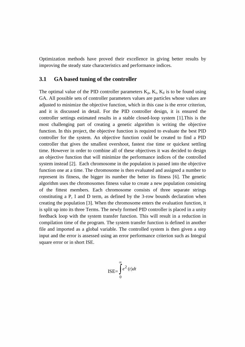
The chromosome is assigned an overall fitness value according to the magnitude of
the error, smaller the error larger the fitness value. Initializing the values of the
parameters is as per Table 1. The flowchart of the GA control system is shown in
figure 2.
Fig.2. Flow Chart of GA.
3.2 EP based tuning of the controller
There are two important ways in which EP differs from GA. First there is no
constraint on the representation. The typical GA approach involves encoding the
problem solutions as a string of representative tokens, the genome. In EP, the
representation follows from the problem. A neural network can be represented in
the same manner as it is implemented. For example, the mutation operation does not
demand a linear encoding [5].
Second, the mutation operation simply changes aspects of the solution according to
a statistical distribution which weights minor variations in the behavior of the
offspring as highly probable and substantial variations as increasingly unlikely. The
steps involved in creating and implementing evolutionary programming are as
follows:
1. Generate an initial, random population of individuals for a fixed size (according
to conventional methods Kp, Ki, Kd ranges declared).
2. Evaluate their fitness (to minimize integral square error). ISE=dtte )(
0
2
3. Select the fittest members of the population.
4. Execute mutation operation with low probability.
5. Select the best chromosome using competition and selection.
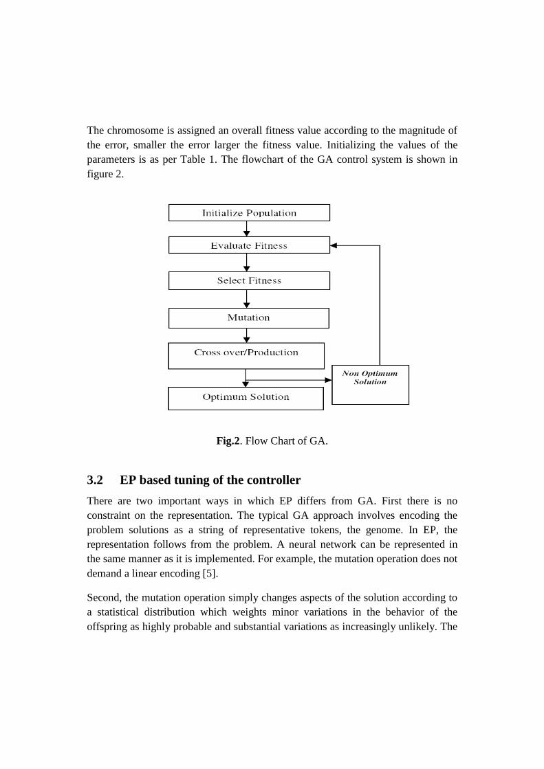
6. If the termination criteria reached (fitness function) then the process ends. If the
termination criteria is not reached, then search for another best chromosome.
The EP parameters chosen are given in Table 1. The flowchart of the EP control
system is shown in figure 3.
Fig.3. Flow Chart of EP
3.3 PSO based tuning of controller
The algorithm proposed by Eberhart and kennedy uses a 1-D approach for searching
within the solution space. For this study the PSO algorithm will be applied to a 2-D
or 3-D solution space in search of optimal tuning parameters for PI, PD and PID
control. The flowchart of the PSO – PID control system [9] is shown in fig
5.Consider position Xi,m of the ith
particle as it traverses a n-dimensional search
space: The previous best position for this ith
particle is recorded and represented as
Pbest I,n. The best performing particle among the swarm population is denoted as
gbest I,n and the velocity of each particle within the n-dimension is represented as
Vi,n. The new velocity and position for each particle can be calculated from its
current velocity and distance respectively [9]. So far (Pbest) and the position in the
d-dimensional space [9]. The velocity of each particle is adjusted accordingly to its
own flying experience and the other particles flying experience [14].
For example, the ith
particle is represented, as xi=(xi 1, xi, 2…….xi, d ) in the d-
dimensional space. The best previous position of the ith
particle is recorded as,
),......,,( ,2,1, diiii PbestPbestPbestPbest
------ (4)
The index of best particle among all of the particles in the group in gbest d .The
velocity for particle i is represented as
)V,.......,V,V(V di,i,2i,1i ------ (5)
The modified velocity and position of each particle can be calculated using the
current velocity and distance from Pbesti,d to gbestd as shown in the following
formulas
))(
,(*()*2
))(
,,(*()*1)(
,.)1(
,
tmixmgbestRandc
tmixmiPbestrandc
tmiVW
tmiV
----- (6)
dmand
nivxxtmi
tmi
tmi
,.....,2,1
,....,2,1)1(
,)(
,)1(
,
------ (7)
Where n is the number of particles in the group, t = Pointer of iterations
(generations),
)(
,
t
miV = Velocity of particle i at iteration t, W is the inertia weight factor, 21,cc are
the acceleration constants,
rand ()=Random number between 0 and 1, )(
,
t
mix is the current position of particle i at
iteration t,,iPbest is the best previous position of the i
th particle and mgbest is the
best particle among all the particles in the population. In the proposed PSO method
each particle contains three members P, I and D. It means that the search space has
three dimension and particles must ‘fly’ in a three dimensional space [9].
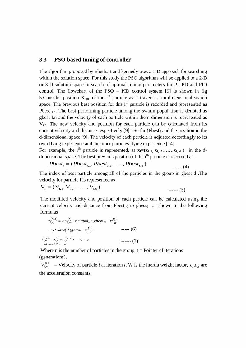
Initializing the values of the parameters is as per Table 1. The flow chart of PSO
control system is shown in Figure 4.
Fig 4. Flowchart of PSO
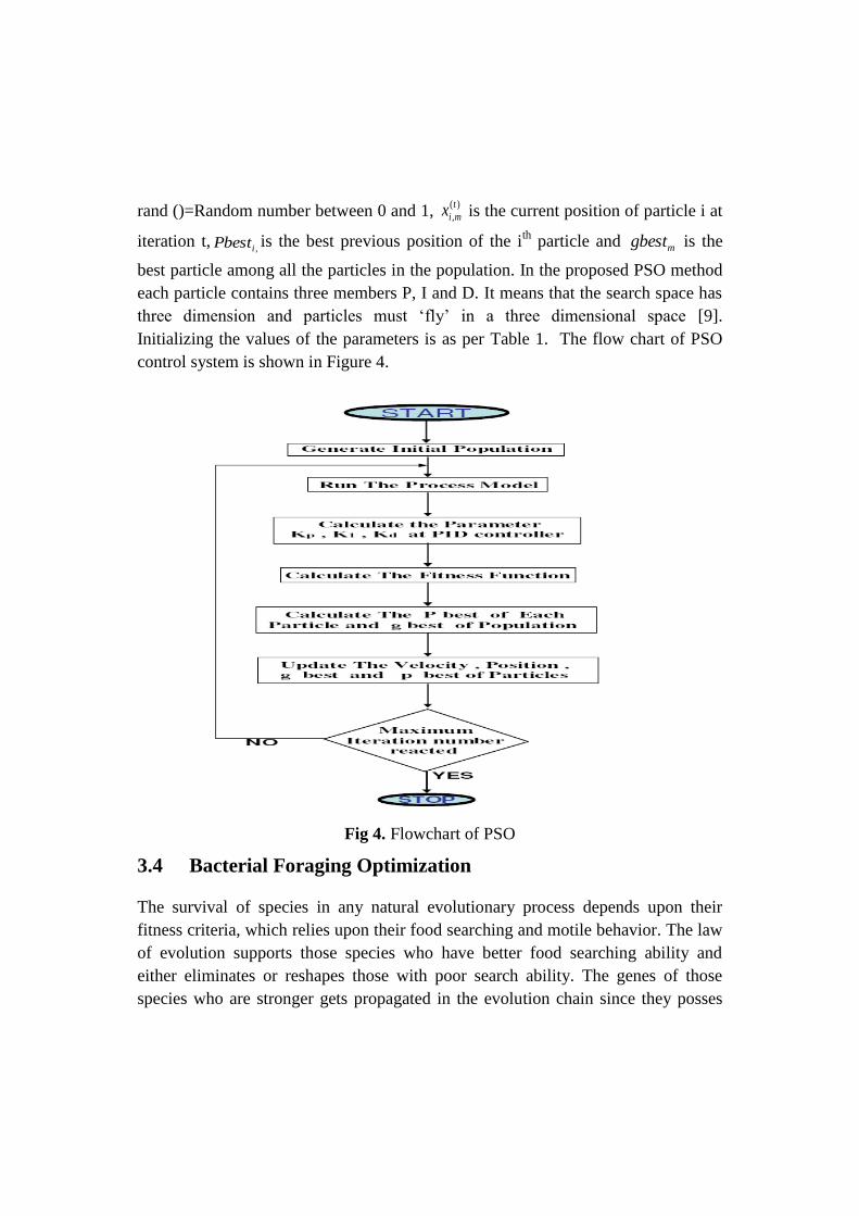
3.4 Bacterial Foraging Optimization
The survival of species in any natural evolutionary process depends upon their
fitness criteria, which relies upon their food searching and motile behavior. The law
of evolution supports those species who have better food searching ability and
either eliminates or reshapes those with poor search ability. The genes of those
species who are stronger gets propagated in the evolution chain since they posses
ability to reproduce even better species in future generations. So a clear
understanding and modeling of foraging behavior in any of the evolutionary
species, leads to its application in any nonlinear system optimization algorithm. The
foraging strategy of Escherichia coli bacteria present in human intestine can be
explained by four processes, namely chemotaxis, swarming, reproduction, and
elimination dispersal [7].
A. Chemotaxis
The characteristics of movement of bacteria in search of food can be defined in two
ways, i.e. swimming and tumbling together known as chemotaxis. A bacterium is
said to be ‘swimming’ if it moves in a predefined direction, and ‘tumbling’ if
moving in a random direction. Mathematically, tumble of any bacterium can be
represented by a unit length of random direction φ (j) multiplied by step length of
that bacterium C(i). In case of swimming, this random length is predefined.
B. Swarming
For the bacteria to reach at the richest food location, it is desired that the optimum
bacterium till a point of time in the search period should try to attract other bacteria
so that together they conquer the desired location more rapidly. To achieve this, a
penalty function based upon the relative distances of each bacterium from the fittest
bacterium till that search duration, is added to the original cost function. Finally,
when all the bacteria have merged into the solution point, this penalty function
becomes zero. The effect of swarming is to make the bacteria congregate into
groups and move as concentric patterns with high bacterial density.
C. Reproduction
The original set of bacteria, after getting evolved through several chemotaxis stages
reaches the reproduction stage. Here, best set of bacteria gets divided into two
groups. The healthier half replaces with the other half of bacteria, which gets
eliminated, owing to their poorer foraging abilities. This makes the population of
bacteria constant in the evolution process [11].
D. Elimination and dispersal
In the evolution process, a sudden unforeseen event can occur, which may
drastically alter the smooth process of evolution and cause the elimination of the
set of bacteria and/or disperse them to a new environment. Most ironically, instead
of disturbing the usual chemo tactic growth of the set of bacteria, this unknown
event may place a newer set of bacteria nearer to the food location. From a broad
perspective, elimination, and dispersal are parts of the population level long
distance motile behavior. In its application to optimization, it helps in reducing the
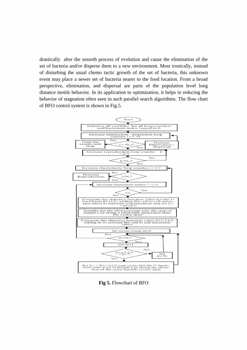
behavior of stagnation often seen in such parallel search algorithms. The flow chart
of BFO control system is shown in Fig.5.
Fig 5. Flowchart of BFO
4 Results and Discussion
A transfer function to validate the process is obtained with the real time data using
Matlab system identification toolbox in equation (1.1-1.3).
Pressure Control System:
--------- (1)
Flow Control System:
15.3224.1
5.6exp5.0
SS
SsflowGP
--------- (2)
Level Control System:
--------- (3)
The tuned values through the traditional, as well as the proposed techniques, are
analyzed for their responses to a unit step input, with the help of Matlab simulation.
A tabulation of the time domain specifications comparison and the performance
index comparison for the obtained models with the designed controllers is
presented. The classical methods such as Zigler Nichol method is employed to find
out the values of Kp, Ki and Kd. Although the classical methods cannot be able to
provide the best solution, they give the initial values or boundary values needed to
start the soft computing algorithms. Due to the high potential of heuristic techniques
such as EP, GA, PSO, BFO methods in finding the optimal solutions, the best
values of Kp, Ki and kd are obtained. The simulations are carried out using
INTEL[R], Pentium [R] CPU 2 GHZ, 1GB RAM in MATLAB 8.0 environment.
The Ziegler-Nichols tuning method using root locus and continuous cycling method
were used to evaluate the PID gains for the system, using the “rlocfind” command
in Matlab, the cross over point and gain of the system were found respectively.
15.0
15.0exp62.0
S
SspressureGP
176.0
5exp02.0
Ss
SslevelGP
Conventional methods of controller tuning lead to a large settling time, overshoot,
rise time and steady state error of the controlled system. Hence Soft computing
techniques is introduces into the control loop. GA, EP, PSO and BFO based tuning
methods have proved their performance in giving better results by improving the
steady state characteristics and performance indices. Performance characteristics of
process were indicated and compared with the intelligent tuning methods as shown
in the figure.6, figure.7 and figure.8 and values are tabulated in table 1, table.2, and
table.3.
4.1 Simulation results for Pressure Control System:
Consider Equ. (1)
TABLE 1.Comparison result of Z-N and Heuristic methods-Pressure System
Tuning
Method
PID Parameters Dynamic performance specifications Performance
Index
Kp
(Proportional
gain)
Ki
(Integral
gain)
T r
(Rise
time)
Ts
(Settling time)
M p (%)
(Peak
overshoot)
ISE
(Integral
square error)
ZN 3 6 3.66 3.68 89% 11.8514
EP 5 40 0.456 6.67 0.2% 0.451
GA 2.4658 4.97 0.971 1.67 0. 0 0.613
PSO 0.5190 0.9531 0.325 0.89 0. 0 0.00281
BFO 1.2989 2.8817 0.156 0.638 0 0.00111
15.0
15.0exp62.0
S
SspressureGP
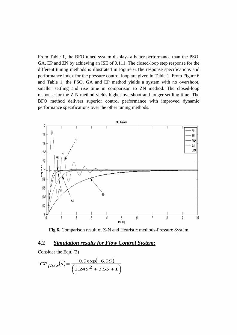
From Table 1, the BFO tuned system displays a better performance than the PSO,
GA, EP and ZN by achieving an ISE of 0.111. The closed-loop step response for the
different tuning methods is illustrated in Figure 6.The response specifications and
performance index for the pressure control loop are given in Table 1. From Figure 6
and Table 1, the PSO, GA and EP method yields a system with no overshoot,
smaller settling and rise time in comparison to ZN method. The closed-loop
response for the Z-N method yields higher overshoot and longer settling time. The
BFO method delivers superior control performance with improved dynamic
performance specifications over the other tuning methods.
Fig.6. Comparison result of Z-N and Heuristic methods-Pressure System
4.2 Simulation results for Flow Control System:
Consider the Equ. (2)
15.3224.1
5.6exp5.0
SS
SsflowGP
From Table 2, the BFO tuned system displays a better performance than the PSO,
GA, EP and ZN by achieving a ISE of 2.2236e-005.The closed-loop step response
for the different tuning methods is illustrated in Figure 7.The response
specifications and performance index for the pressure control loop are given in
Table 2. From Figure 7 and Table 2, the PSO, GA and EP method yields a system
with marginally higher overshoot, longer settling and rise time in comparison to
BFO method. The closed-loop response for the Z-N method yields higher overshoot
and longer settling time. The BFO method delivers superior control performance
with improved dynamic performance specifications over the other tuning methods.
TABLE 2.Comparison result of Z-N and Heuristic methods-Flow system
Tuning
Method
PID Parameters Dynamic performance specifications Performance
Index
Kp
(Proportional
gain)
Ki
(Integral
gain)
T r
(Rise time)
Ts
(Settling
time)
M p (%)
(Peak
overshoot)
ISE
(Integral
square error)
ZN 0.6 0.25 9.6 82.2 39.6 8.56
EP 0.456 0.12 19.1 40.4 8.45 2.5
GA 0.4 0.123 17.7 37.2 5.57 0.0054
PSO 0.6 0.17 10 33.8 0.218 4.2849e-006
BFO 0.7 0.1689 9.6 32.1 0 2.2236e-005
Fig.7. Comparison result of Z-N and Heuristic methods-Flow System
4.3 Simulation results for Level Control System:
Consider the Equ. (3)
176.0
5exp02.0
Ss
SslevelGP
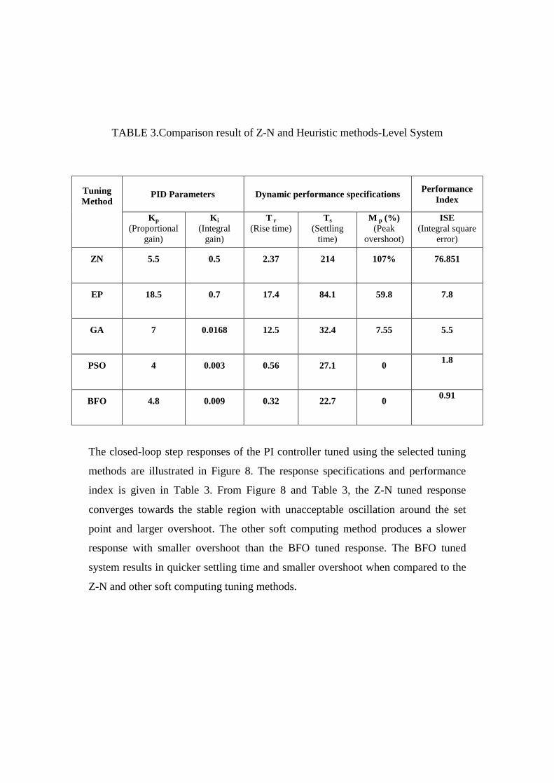
TABLE 3.Comparison result of Z-N and Heuristic methods-Level System
The closed-loop step responses of the PI controller tuned using the selected tuning
methods are illustrated in Figure 8. The response specifications and performance
index is given in Table 3. From Figure 8 and Table 3, the Z-N tuned response
converges towards the stable region with unacceptable oscillation around the set
point and larger overshoot. The other soft computing method produces a slower
response with smaller overshoot than the BFO tuned response. The BFO tuned
system results in quicker settling time and smaller overshoot when compared to the
Z-N and other soft computing tuning methods.
Tuning
Method
PID Parameters Dynamic performance specifications Performance
Index
Kp
(Proportional
gain)
Ki
(Integral
gain)
T r
(Rise time)
Ts
(Settling
time)
M p (%)
(Peak
overshoot)
ISE
(Integral square
error)
ZN 5.5 0.5 2.37 214 107% 76.851
EP 18.5 0.7 17.4 84.1 59.8 7.8
GA 7 0.0168 12.5 32.4 7.55 5.5
PSO 4 0.003 0.56 27.1 0 1.8
BFO 4.8 0.009 0.32 22.7 0 0.91
Fig.8. Comparison result of Z-N and Heuristic methods-Level System
5 Conclusion
The ZN, GA, EP, PSO, and BFO tuning methods have been implemented on
pressure, flow and level control loops and a comparison of control performance
using these methods has been completed. For the Z-N controller set point tracking
performance is characterized by lack of smooth transition as well it has more
oscillations. Also it takes much time to reach set point. The Soft computing based
controller tracks the set point faster and maintains steady state. It was found for all
control loops the performance of the Soft computing based controller was much
superior to the Z-N control. Soft computing techniques are often criticized for two
reasons: Algorithms are computationally heavy and convergence to the optimal
solution cannot be guaranteed. PID controller tuning is a small-scale problem and
thus computational complexity is not really an issue here. It took only a couple of
seconds to solve the problem. Compared to conventionally tuned system, BFO
tuned system has good steady state response and performance indices.
References
[1] Valarmathi1, D. Devaraj, T. K. Radhakrishnan, Chemical Engineering ,Vol.
26, (2009), pp. 99 – 111.
[2] Andrey Popov, Adel Farag, Herbert Werner, 44th IEEE Conference on
Decision and Control, pp. 7139-7143.
[3] A. Andrášik, A. Mészáros, A. Azevedob,Compchemeng , Vol.28 (2004) ,
pp. 1499-1509
[4] Mohammed El-Said El-Telbany, ICGST-ACSE, Vol. 7, (2007), 49-54.
[5] Jukka Lieslehto American Control Conference, VA, (2001), pp. 2828-2833.
[6] Maolong Xi,Jun Sun,
Wenbo Xu, Modeling , Control and Simulation ,
pp. 603-607.
[7] S.Nithya, N.Sivakumaran, T.K.Radhakrishnan and N.Anantharaman,
WCECS, Vol. 2 (2010).
[8] Dong Hwa Kim , Ajith Abraham, Jae Hoon Cho, Information Sciences 177
(2007) , pp. 3918-3937
[9] Dong Hwa Kim, Jae Hoon Cho, IJCAS, vol. 4, no. 5, (2006). pp. 624-636
[10] S.M.GirirajKumar, R.Sivasankar,T.K.Radhakrishnan,V.Dharmalingam,and
Anantharaman, Instrumentation Science and Technology, 36: (2008), pp.
525–542,
[11] K. J. Astrom, T. Hagglund, Control Engineering Practice, Vol. 9, No.11,
(2001), pp. 1163-1175
[12] T. S. Schei, Automatica, 30, No-12, (1994),pp. 1983-1989.
[13] K. Ramkumar, O.V Sanjay Sharma, International journal of computer
application , Vol. 3, (2010), pp. 34-46.
[14] Hyung-soo Hwang, Jeong-Nae Choi, Won-Hyok Lee: IEEE Proceedings
(1999), pp. 2210-2215.
[15] K.M. Passino, IEEE Control Systems Magazine, Vol. 22, (1989), pp. 44-52.
[16] S. Mishra, IEEE Trans. Evolutionary Computation,Vol. 9,(2005), pp. 61-73.
[17] D. H. Kim, A. Abraham and J. H. cho, Inf.Sci,Vol. 177, (2007), pp. 3918-
3937.
[18] K. J. Astrom, Journal of Process Control, Vol. 14, (2004), pp. 635-650
[19] K. E. Parsopoulos, M. V. Vrahatis. IEEE Trans Evolutionary Computation;
8(3), (2004), pp. 211-24
[20] J. Robinson, Y.R. Samii, IEEE Trans Antenn Propag; 52(2), (2004), pp.
397-407.
[21] Amir Atapour Abarghouei, Afshin Ghanizadeh, and Siti Mariyam
Shamsuddin. Advances of Soft Computing Methods in Edge Detection, Int.
J. Advance. Soft Comput. Appl., Vol. 1, No. 2, pp. 164-201.
[22] K. Premalatha, A.M. Natarajan. Hybrid PSO and GA Models for Document
Clustering, Int. J. Advance. Soft Comput. Appl., Vol. 2, No. 3, pp. 302-320.