CONTROLLING MIXING AND SEGREGATION IN TIME PERIODIC GRANULAR FLOWS by Tathagata Bhattacharya Master of Technology, Indian Institute of Technology (IIT), Kanpur, India, 2002 Bachelor of Engineering, The University of North Bengal, Darjeeling, India, 2000 Submitted to the Graduate Faculty of the Swanson School of Engineering in partial fulfillment of the requirements for the degree of Doctor of Philosophy University of Pittsburgh 2011
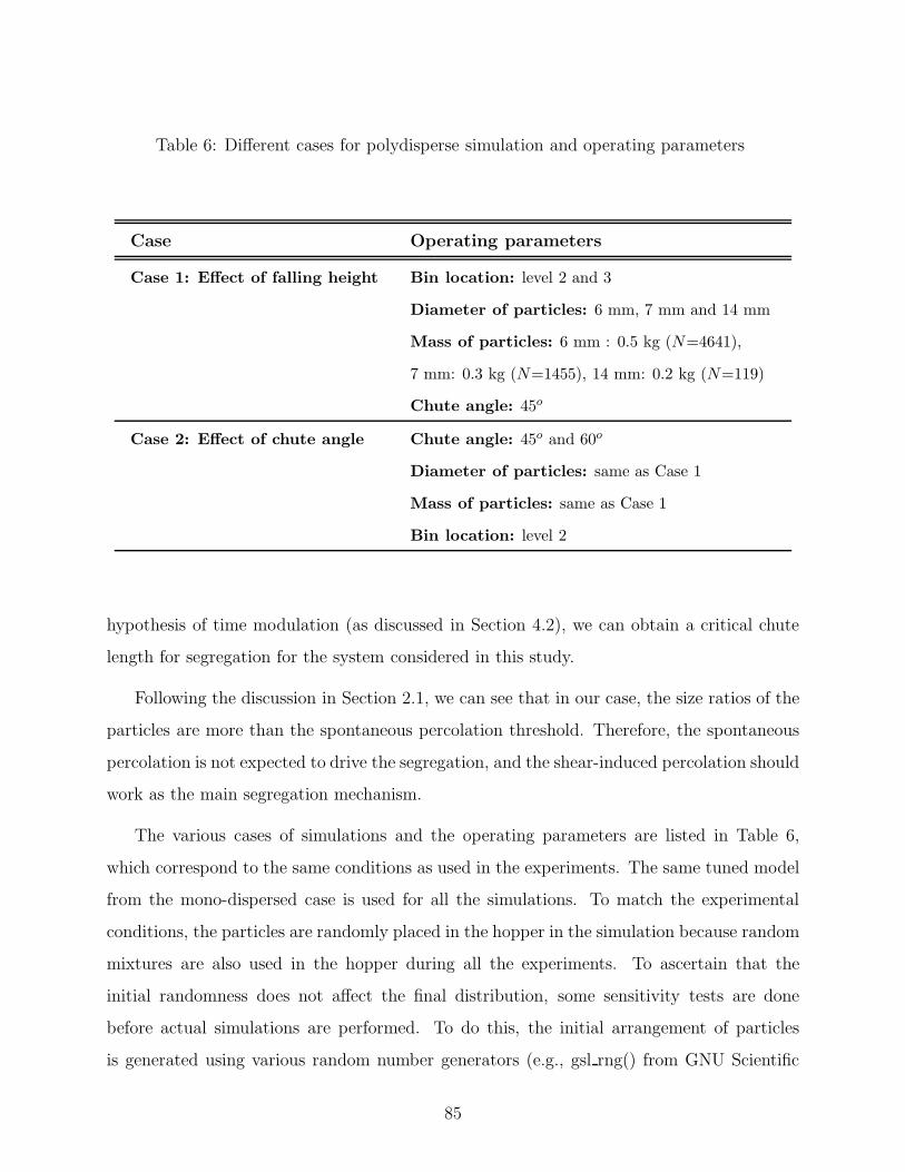
Transcript
CONTROLLING MIXING AND SEGREGATION IN
TIME PERIODIC GRANULAR FLOWS
by
Tathagata Bhattacharya
Master of Technology, Indian Institute of Technology (IIT),
Kanpur, India, 2002
Bachelor of Engineering, The University of North Bengal,
Darjeeling, India, 2000
Submitted to the Graduate Faculty of
the Swanson School of Engineering in partial fulfillment
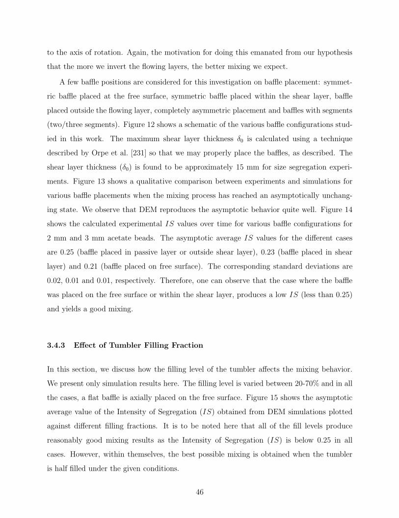
of the requirements for the degree of
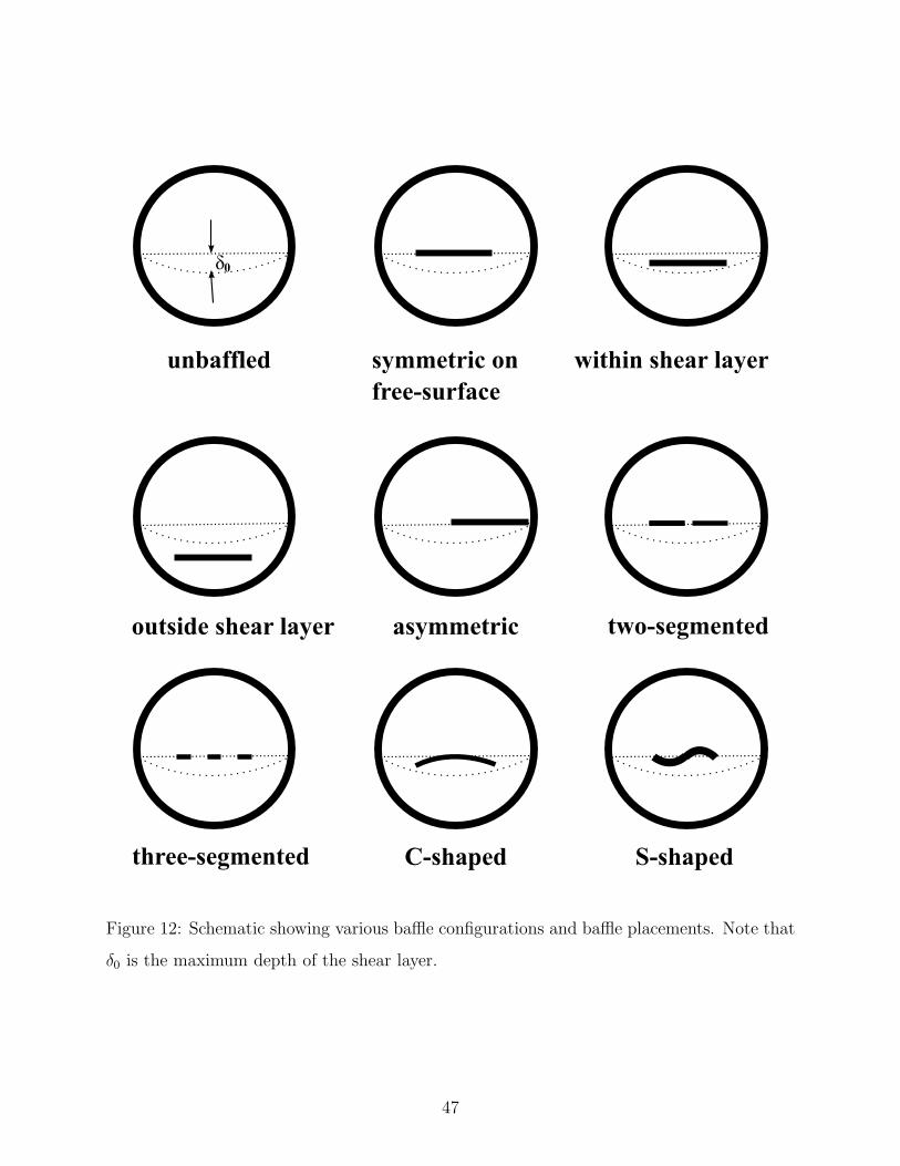
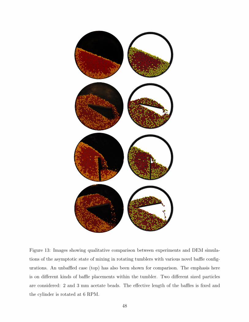
Doctor of Philosophy
University of Pittsburgh
2011
UNIVERSITY OF PITTSBURGH
SWANSON SCHOOL OF ENGINEERING
This dissertation was presented
by
Tathagata Bhattacharya
It was defended on
September 22, 2011
and approved by
Joseph J. McCarthy, Ph.D., Professor, Department of Chemical and Petroleum Engineering
Robert S. Parker, Ph.D., Associate Professor, Department of Chemical and Petroleum
Engineering
Sachin S. Velankar, Ph.D., Associate Professor, Department of Chemical and Petroleum
Engineering
Albert C. To, Ph.D., Assistant Professor, Department of Mechanical Engineering and
Materials Science
Dissertation Director: Joseph J. McCarthy, Ph.D., Professor, Department of Chemical and
5 Total contact detection time as a function of total number of particles. [◦]corresponds to our implementation of the original NBS algorithm of Munjiza
et al. [3] in C and [•] corresponds to the modification of the outer loop of the
NBS algorithm using an efficient data structure in C++. A naive brute force
method where all particles are searched against all other particles has also been
included. Total contact detection time has been obtained by running the outer
loop 10 times in a 3.2 GHz, Intel Xeon processor. . . . . . . . . . . . . . . . . 27
6 Different regimes of flow in a rotating drum (illustration obtained from Var-
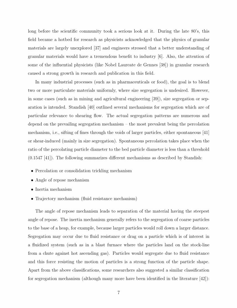
The angle of repose mechanism leads to separation of the material having the steepest
angle of repose. The inertia mechanism generally refers to the segregation of coarse particles
to the base of a heap, for example, because larger particles would roll down a larger distance.
Segregation may occur due to fluid resistance or drag on a particle which is of interest in
a fluidized system (such as in a blast furnace where the particles land on the stock-line
from a chute against hot ascending gas). Particles would segregate due to fluid resistance
and this force resisting the motion of particles is a strong function of the particle shape.
Apart from the above classifications, some researchers also suggested a similar classification
for segregation mechanism (although many more have been identified in the literature [42]):
7
percolation/sieving, fluidization, convection, and trajectory segregation. These four mech-
anisms are nearly similar to the ones proposed by Standish [40] and share many common
features. They have been pictorially described in Figure 1.
Amongst the early literature [13, 14, 28, 43–48], Drahun et al. [49] seem to be the first
workers who have done extensive experimentation on this particular topic by analyzing the
effects of various variables on segregation. They have reported comprehensive findings on the
mechanism of free surface segregation along a slope, which can be helpful in understanding
exactly the same phenomena occurring in a tumbler or in a chute flow. Their report also con-
tained an assessment of previous work (15 references therein) performed on the mechanism
of segregation. They observed that although the existence of free surface segregation had
long been recognized, there had been few attempts to produce theories that would predict
quantitatively the amount of segregation. Most investigators were primarily interested in the
prevention of segregation rather than the factors that caused it. Therefore, attempts were
made to solve a particular problem on an ad-hoc basis without fundamental understanding
of its occurrence. Moreover, the results of some of the studies are not generic and are not
applicable universally. Drahun et al. noted that, in general, analytical models do not cap-
ture the key features of free surface segregation satisfactorily (e.g., the predictive models by
Matthee [45] and Tanaka [46]). Drahun et al.’s study was conducted with binary systems
where one component was present in small quantities. The experimental setup permitted
the slope length, solids flow rate and solids fall height to be varied independently in order
to assess the effects of independent variables (e.g., size, density, shape, free fall height, etc.)
on the rate and extent of segregation. Results were presented in dimensionless form and the
major findings from their work are summarized below:
• Free surface segregation occurs by avalanching, inter-particle percolation and particle
migration.
• Both diameter and density have a significant effect on segregation. Smaller particles sink
by percolation and are found closer to the pouring point, whereas large particles rise to
the surface by particle migration and are found at the extreme end of the surface. On
the other hand, the denser particles are found near the pouring point and less dense
particles at the far end. This gives rise to stratification.
8
Figure 1: Various segregation mechanisms (illustration obtained from Figueroa [1] with
permission).
9
• An increase in particle velocity onto the inclined surface influences the material distribu-
tion controlled by diameter but not that controlled by density. In particular, if the free
fall height is increased, the smaller particles bounce down the free surface to the far end.
• A slight segregation in a feeding device like conveyor or hopper can markedly influence
the free surface segregation.
• Free surface segregation can be minimized by appropriate balance of size ratio and density
ratio.
• Particle shape, unless extreme such as needles or platelets, does not have much effect on
segregation.
• Surface roughness or the surface friction arising out of the shape has no effect on segre-
gation. Rolling and sliding do not contribute greatly to segregation.
Recently, Makse et al. [50] has provided some explanations to the above mentioned phe-
nomena, especially, stratification or layering. When poured between two vertical plates, a
granular mixture spontaneously stratifies into alternating layers of small and large particles
whenever the large particles have larger angle of repose than the small ones. Makse et al.
also found spontaneous segregation, without stratification, when the large particles have
smaller angle of repose than the small ones.
Tanaka et al. [46] developed a first principle 2D mathematical model, which is capable
of describing the movement of only two particles relative to one another using a critical
friction coefficient as the determining factor for one of the two particles’ movement. It
was originally used to quantify the segregation phenomena in flows from hoppers. This
model was later modified by Kajiwara et al. [51] and Tanaka et al. [52] to analyze the
segregation phenomena in an industrial process: Distribution of coke and iron ore at the
top of a blast furnace. The mathematical model used a discrete approach to analyze the
granular flow problem. In their work, the distinct (or discrete) element method (DEM)
technique was employed. The constitutive equation for interaction between two particles
was described by a Voigt-Kelvin rheological model with a slider and dashpot. Previously,
Cundall and Strack (1979) [2] described a similar discrete model to capture the behavior of
an assembly of particles, but they did not employ a viscous effect when approximating the
sliding condition. Later, Kajiwara et al. [51] used a slider and dashpot, which represented
10
the kinetic energy dissipation of particles, and the accuracy of the model was enhanced.
In their study, the dashpot factor was experimentally determined. In their report, the
authors cited a few references where different techniques were reviewed and their drawbacks
in effectively modeling the flow dynamics of granular material were mentioned. They found
that there is extensive literature on the flow of granular materials under the assumption of
continuum, but those studies lack generality and cannot capture the segregation phenomena
with higher analytical accuracy. Kajiwara et al. also claimed that their work has led to a
better understanding of the solids flow in the process and can remove the inherent difficulties
in a continuum approach. Their model was used to examine segregation during discharge
from a hopper. Specifically, they analyzed the particle size distribution when a stone box
(one type of insert) was used in the hopper: the stone box suppressed the variation of
particle size distribution during discharge in the radial direction. Kajiwara et al.’s model
also precisely described the frictional wall effect in solids flow and bridge formation. In a
nutshell, this work was one of the first computational efforts to apply DEM to understand
the segregation phenomena in an industrial process.
Since DEM is computationally demanding, Kajiwara and Tanaka’s group developed an-
other model [53] based on percolation theory to examine the sieving behavior of smaller
particles on a slope and to study segregation. The percolation frequency of the small par-
ticle is determined by particle size ratio and the velocity gradient. Earlier, Bridgwater et
al. [48] had shown the functional behavior of this percolation frequency using experiments.
There have been many efforts to model the free surface segregation in simple shear flows
(such as in pile/heap formation) based on continuum principles. Some of the first studies
were done by Bouchaud et al. (BCRE model, after Bouchaud, Cates, Ravi and Edwards) [54]
and Mehta et al. [55]. In the BCRE model, they considered single-species sandpile (no
segregation) and used two coupled variables to describe the evolution of sand piles. The
two variables were the height of the sand pile h(x, t) (which corresponds to static bed), and
the local thickness of the rolling layer, R(x, t). BCRE also proposed a set of convective-
diffusion equations for the rolling grains, which was later simplified by de Gennes [56].
Recently, Boutreux and de Gennes (BdG model) [57] extended the BCRE model for the case
of two species (the so-called “minimal” model). In this model, grains with different surface
11
properties but of equal size were considered. Since the minimal model does not take into
account the size difference between the grains, Boutreux had treated the important case
(the so-called “canonical” model) where the grains differed only in size (surface properties
being the same), in a second article [58,59] of the series started by BdG [57]. Boutreux [59]
argued that unlike Makse et al. [60] (whose modification of first BdG model [57] applies
only to a case with large difference of size), their generalization is applicable for situations
where the species have a small difference of sizes. In the last and third paper of the BdG
series [61], Boutreux et al. presented the generalization of the minimal model for surface
flows of granular mixtures (referred to as the general case of the canonical model). The final
model [61] takes into account both the differences in surface properties and the size of the
grains.
More recently, Jop, Forterre and Pouliquen [62] proposed a constitutive law for dense
granular flows based on continuum method using a simple visco-plastic approach. They
observed that a continuum description of free surface flows is at present debatable because
of the fact that granular materials can behave [26] like a solid (in a sand pile), a liquid (when
poured from a silo) or a gas (when strongly agitated). For the two limiting cases, solids
and gases, constitutive equations have been proposed based on kinetic theory for collisional
rapid flows, and soil mechanics for slow plastic flows. The intermediate dense regime, where
the granular material flows like a liquid, still lacks a unified view and has motivated many
studies over the past decade. Though Jop et al.’s work [62] does not consider any difference in
particle sizes (no segregation), it is a step forward in developing continuum based segregation
models. Additional work along this line can be found in a recent review by Campbell [63].
The above paragraphs provide a general background of the free surface segregation.
Review of the segregation phenomena pertaining to a specific system such as in a rotating
tumbler and in a chute is presented in the corresponding chapters. In the next section, for
completeness, we briefly review the numerical techniques used in the direct simulations of
granular flow systems in this dissertation.
12
2.2 MODELING: PARTICLE DYNAMICS
Particle dynamics (PD), which is also known as the discrete element method (DEM), has
been quite successful in simulating granular materials [64–76], yielding insight into such
diverse microscopic phenomena as force transmission [77], packing [78], wave propagation
[70], agglomeration formation and breakage [79], cohesive mixing [80], bubble formation in
fluidized beds [72], and segregation of free-flowing materials [21]. This method, originally
developed by Cundall and Strack in 1979 [2], is based on the methodology of molecular
dynamics (MD) for the study of liquids and gases (Allen and Tildesley, 1987 [81]). A recent
review (up to the year 2006) on particle dynamics theory and its applications can be found
in Zhu et al. [82] and in Zhu et al. [64], respectively. The basic advantage of particle
dynamics over continuum techniques is that it simulates effects at the particle level owing
to its first-principle nature (“exact numerical experiment” [16]). No global assumption is
needed as is customary in a continuum description. Individual particle properties can be
specified directly, and the assembly performance, like segregation, is simply an output from
the simulation. Also, the growth of this technique can be attributed, in part, to the ever
increasing speed of modern computers.
Currently, a million particles can be easily simulated using high performance computing
(HPC) which involves the application of highly scalable parallel processing and tremendous
acceleration from general purpose GPUs (graphics processing units) [83] to push the com-
putation power to petascale levels. Roth et al., 2000 [84] and Kadau et al., 2006 [85] have
already demonstrated this with billions of particles in a molecular dynamics run. Though
particle dynamics (PD) algorithms are similar in structure with molecular dynamics (MD),
PD simulations are computationally more expensive due to the peculiar interaction of gran-
ular particles: Particles exert forces on each other only when they are in mechanical contact.
In MD, particles can interact even when they are not in mechanical contact (influence zone
of particles is defined by a “cut-off” distance). This “cut-off” distance in MD is usually
more than PD (in PD, it is summation of the contacting particles radii). The computational
intensity is also aggravated by the fact that the granular particles are rather rigid and their
repulsive force grows steeply with the compression once the particles are in contact. This
13
condition dictates a very small integration time step for the computation of the trajectories
in order to obtain reliable results.
This section is organized as follows: First we discuss a general DEM algorithm, then two
important parts of a DEM algorithm are elicited – contact force modeling and the contact
detection algorithm.
2.2.1 General DEM Algorithm
2.2.1.1 Hard-sphere vs. Soft-sphere Depending on the bulk density and characteris-
tics of the flow to be modeled, two different methods of calculating the trajectories are used:
Hard-sphere model and soft-sphere model.
The hard-sphere model works in rapid, not-so-dense flows (like “granular gases” [86])
where the collisions are instantaneous (i.e., duration of a collision, tc = 0) and the typical
duration of a collision is much shorter than the mean time between successive collisions.
While in a true “dilute flow”, particles only rarely experience multi-body interactions, in this
technique they cannot be in contact with more than one other particle. As the name suggests,
the particles do not suffer any deformation to generate the contact forces. The central idea of
hard-sphere modeling is to track the next collisions and the particle trajectories are obtained
from a set of collision rules (no integration is performed) which relate the post-collision
velocities as a function of pre-collision velocities (using coefficient of restitution, both for
normal and tangential directions). Hence, during the time intervals between collisions, the
particles move along known ballistic trajectories. In this regime, one applies the conservation
of linear and angular momentum for each collision sequentially – one collision at a time [87].
This method is also known as an “event-driven” algorithm. At low particle concentration,
this algorithm is much more efficient than force-based soft-sphere method since the numerical
integration of the equations of motion is avoided. Instead, the dynamics of the system is
determined by a sequence of discrete events. The enormous gain in the simulation speed is
the main motivation for using this approach.
However, in this dissertation, we employ a soft-sphere approach owing to the fact that
our systems can be characterized by slow, dense granular flows where particles have enduring
14
contacts and multi-particle collisions are highly likely. As the name suggests, the particles
can deform and forces arise because of this deformation. As will be discussed in the next sub-
section, particle trajectories are obtained via integration of forces at discrete time intervals
as the simulation marches forward in time. That is why this method is also known as
“time-step-driven” simulation.
2.2.1.2 Equations of Motion In the soft-sphere PD or DEM model (we use PD or
DEM interchangeably or synonymously throughout this document), bulk flow of the granular
materials is captured via simultaneous integration of the interaction forces between individual
pairs of particles in contact, and the trajectories are obtained by explicit solution of Newton’s
equations of motion for every particle [2, 81].
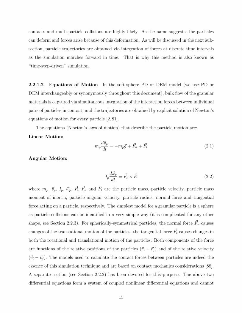
The equations (Newton’s laws of motion) that describe the particle motion are:
Linear Motion:
mpd~vpdt
= −mp~g + ~Fn + ~Ft (2.1)
Angular Motion:
Ipd~ωp
dt= ~Ft × ~R (2.2)
where mp, ~vp, Ip, ~ωp, ~R, ~Fn and ~Ft are the particle mass, particle velocity, particle mass
moment of inertia, particle angular velocity, particle radius, normal force and tangential
force acting on a particle, respectively. The simplest model for a granular particle is a sphere
as particle collisions can be identified in a very simple way (it is complicated for any other
shape, see Section 2.2.3). For spherically-symmetrical particles, the normal force ~Fn causes
changes of the translational motion of the particles; the tangential force ~Ft causes changes in
both the rotational and translational motion of the particles. Both components of the force
are functions of the relative positions of the particles (~ri − ~rj) and of the relative velocity
(~vi − ~vj). The models used to calculate the contact forces between particles are indeed the
essence of this simulation technique and are based on contact mechanics considerations [88].
A separate section (see Section 2.2.2) has been devoted for this purpose. The above two
differential equations form a system of coupled nonlinear differential equations and cannot
15
be solved analytically (cannot be directly integrated). The approximate numerical solutions
of these equations, i.e., the computation of the trajectories of all particles of the system by
numerical integration is the ultimate objective of DEM. We elaborate on the integration
scheme and general flow of our DEM algorithm in the next sections.
2.2.1.3 Boundary Conditions Just as a problem in continuum mechanics needs initial
and boundary conditions (the similarity between continuum mechanics and discrete system
is that we start with a system of differential equations, and hence initial and boundary
conditions are needed for both to solve), the description of a particle system is complete
only when the behavior of the particles at the boundary is properly described and if the
initial conditions, both particle coordinates and velocities, are supplied.
For our boundary conditions, we use both periodic and wall boundaries. The wall bound-
ary is obtained by building up the walls from particles which obey the same rules of interac-
tion as the particles of the granular materials themselves. By choosing appropriate sizes and
positions of the wall particles, boundaries (like container walls, inclined surfaces, etc.) with
adjustable roughness can be obtained. This kind of boundary can be easily incorporated in
the DEM algorithm without needing any extra interaction rules – the particle-particle force
laws can still be applied to the walls too. The wall or boundary particles do not interact with
each other and they can have a prescribed motion (like rotation). An alternative to the use
of boundary/wall particles is the use of mathematical smooth walls (flat surfaces); however,
the use of these types of walls necessitates special treatment, such as rolling friction, which
we will discuss briefly later. Our simulations are periodic in the z direction so that any par-
ticle which leaves the system at one side is re-inserted at the opposite side. Such boundary
conditions are used to mimic infinitely extended systems (i.e., a cylinder with a periodic
z direction is equivalent to a cylinder with infinite length). Algorithmic implementation
of periodic boundary conditions is rather simple in granular systems (PD) as the particle
interactions (forces) are short-ranged (as opposed to MD).
2.2.1.4 Initial Conditions Coming back to the initial conditions for DEM, the values
of the coordinates ~rp(t = 0), the velocities ~vp(t = 0) and angular velocities ~ωp(t = 0) should
16
be specified for p = 1, ..., N , where N is the total number of particles in the system. A typical
initial condition for our simulations is obtained by allowing a bed of particles arranged in
a randomly perturbed lattice to settle under the action of gravity so that a relaxed state is
obtained. Initial positioning of the particles in the lattice sites should avoid large overlaps
as this would generate very large spurious forces, which are unrealistic, and the simulation
would not proceed further.
2.2.1.5 Integration Scheme and Time-Step Now we turn our attention to the inte-
gration scheme and time-step used in our algorithm. From the position of particles, all forces
acting on each particle are determined and the net acceleration of the particle is obtained,
both linear and angular. The position and orientation at the end of next time-step is then
evaluated explicitly using the method of integration (one type of “finite-difference” method)
initially adopted by Verlet and attributed to Stormer [81] :
xt+ 1
2∆t = xt +
1
2xt∆t (2.3)
xt+∆t = xt +1
2(xt + xt+∆t)∆t (2.4)
The time-step ∆t should be chosen to be sufficiently small such that any disturbance
(in this case a displacement-induced stress on a particle) does not propagate further than
that particle’s immediate neighbors within one time-step. Generally, this criterion is met
by choosing a time-step which is smaller than r/λ, where r is the particle radius and λ
(λ ∝√
E/ρ) represents the relevant disturbance wave speed (for example, dilatational,
distortional or Rayleigh waves [68]). Under these conditions, the method becomes explicit,
and therefore at any time increment the resultant forces on any particle are determined
exclusively by its interaction with the closest neighbors in contact. Thornton and Randall [68]
suggest the time-step be chosen to correspond with Rayleigh wave speed (∝√
Gρ) so that
∆t =πR
αo
√
ρ
G(2.5)
17
where R is the particle radius, αo is a constant (taken to be 0.1631ν + 0.8766 in our case),
ρ is the density of the particle and G is the shear modulus, and ν is the Poisson ratio of the
particle. To be on the safe side, we have used one quarter of the time-step value given by
the above Equation 2.5, which yielded a time-step ∆t ≈ 10−6 s.
A flow chart of the DEM algorithm is given in Figure 2.
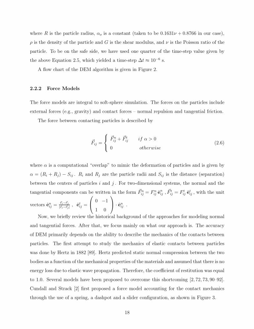
2.2.2 Force Models
The force models are integral to soft-sphere simulation. The forces on the particles include
external forces (e.g., gravity) and contact forces – normal repulsion and tangential friction.
The force between contacting particles is described by
~Fij =
~F nij +
~F tij if α > 0
0 otherwise(2.6)
where α is a computational “overlap” to mimic the deformation of particles and is given by
α = (Ri + Rj) − Sij . Ri and Rj are the particle radii and Sij is the distance (separation)
between the centers of particles i and j . For two-dimensional systems, the normal and the
tangential components can be written in the form ~F nij = F n
ij enij , ~F
tij = F t
ij etij , with the unit
vectors enij =~ri−~rj|~ri−~rj |
, etij =
0 −1
1 0
· enij .
Now, we briefly review the historical background of the approaches for modeling normal
and tangential forces. After that, we focus mainly on what our approach is. The accuracy
of DEM primarily depends on the ability to describe the mechanics of the contacts between
particles. The first attempt to study the mechanics of elastic contacts between particles
was done by Hertz in 1882 [89]. Hertz predicted static normal compression between the two
bodies as a function of the mechanical properties of the materials and assumed that there is no
energy loss due to elastic wave propagation. Therefore, the coefficient of restitution was equal
to 1.0. Several models have been proposed to overcome this shortcoming [2, 72, 73, 90–92].
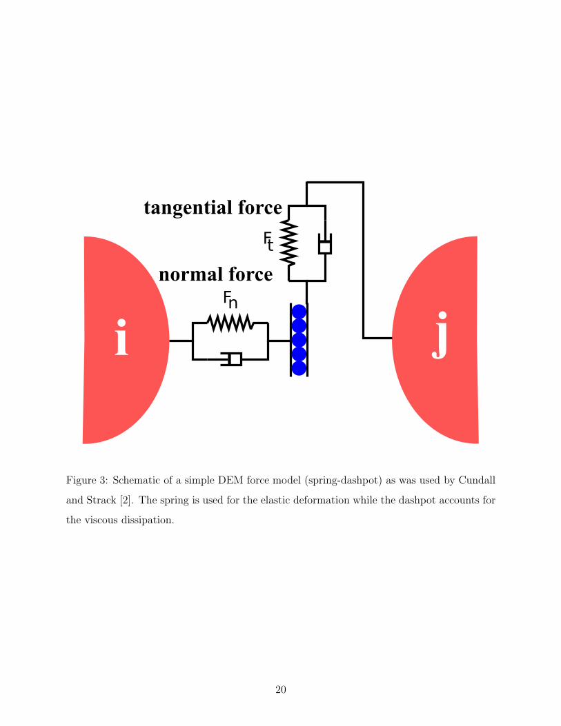
Cundall and Strack [2] first proposed a force model accounting for the contact mechanics
through the use of a spring, a dashpot and a slider configuration, as shown in Figure 3.
18
Contact Check
Interparticle Forces
Increment
Velocity and Coordinate
Update
t = t + dt
Generate Particles
Figure 2: Flow chart of a typical DEM algorithm.
19
nF
Ft
i j
normal force
tangential force
Figure 3: Schematic of a simple DEM force model (spring-dashpot) as was used by Cundall
and Strack [2]. The spring is used for the elastic deformation while the dashpot accounts for
the viscous dissipation.
20
Walton and Braun proposed a normal contact model which was able to mimic elasto-
plastic and plastic collisions giving restitution coefficients in good agreement with experi-
mental results [73]. With respect to tangential loads between particles, Mindlin and Dere-
siewicz [93] described the microslip and sliding processes as a result of variable normal and
tangential forces. The deformation is contact history dependent and contact mechanics
models with different approaches have been proposed [2, 68, 72, 79].
A thorough description of the interaction laws from contact mechanics and their merits
can be found in references [82,94–97]; therefore, they are not reviewed here. We only discuss
the models employed in the present work.
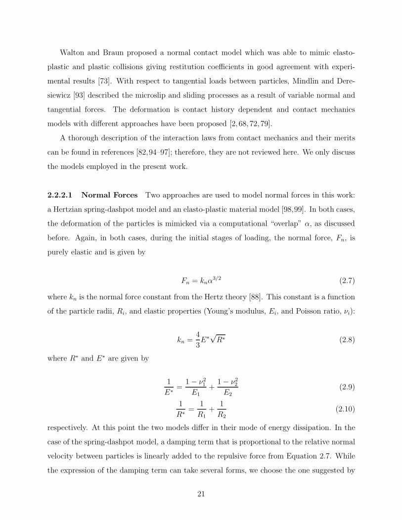
2.2.2.1 Normal Forces Two approaches are used to model normal forces in this work:
a Hertzian spring-dashpot model and an elasto-plastic material model [98,99]. In both cases,
the deformation of the particles is mimicked via a computational “overlap” α, as discussed
before. Again, in both cases, during the initial stages of loading, the normal force, Fn, is
purely elastic and is given by
Fn = knα3/2 (2.7)
where kn is the normal force constant from the Hertz theory [88]. This constant is a function
of the particle radii, Ri, and elastic properties (Young’s modulus, Ei, and Poisson ratio, νi):
kn =4
3E∗
√R∗ (2.8)
where R∗ and E∗ are given by
1
E∗=
1− ν21
E1+
1− ν22
E2(2.9)
1
R∗=
1
R1+
1
R2(2.10)
respectively. At this point the two models differ in their mode of energy dissipation. In the
case of the spring-dashpot model, a damping term that is proportional to the relative normal
velocity between particles is linearly added to the repulsive force from Equation 2.7. While
the expression of the damping term can take several forms, we choose the one suggested by
21
Oden and Martins [91] due to the fact that it qualitatively reproduces the experimentally
observed dependence of the coefficient of restitution on impact velocity for many engineering
materials (i.e., a power law decrease). Combining the repulsive force and this dissipation
term yields what we refer to as our elastic model henceforth, given as
Fn = knα3/2 − γnαα (2.11)
where α is the relative normal velocity (vn) of the particles, and γn is a damping parameter
that is assumed to be adjustable and is simply supplied as a constant in the model (we used
γn = 0.0015E1−ν2
).
In contrast, in our elasto-plastic model (referred to as plastic model henceforth), dissi-
pation is assumed to arise from the plastic deformation of the center of the contact spot. In
this model, once the normal force exceeds a yield force, Fy, further loading is given by the
linear expression
Fn = Fy + ky(α− αy) (2.12)
In this expression, ky is the plastic stiffness which is related to the yield force by ky =
(3/2)(Fy/αy), and αy is the deformation at the point of yield (i.e., where both Equation 2.7
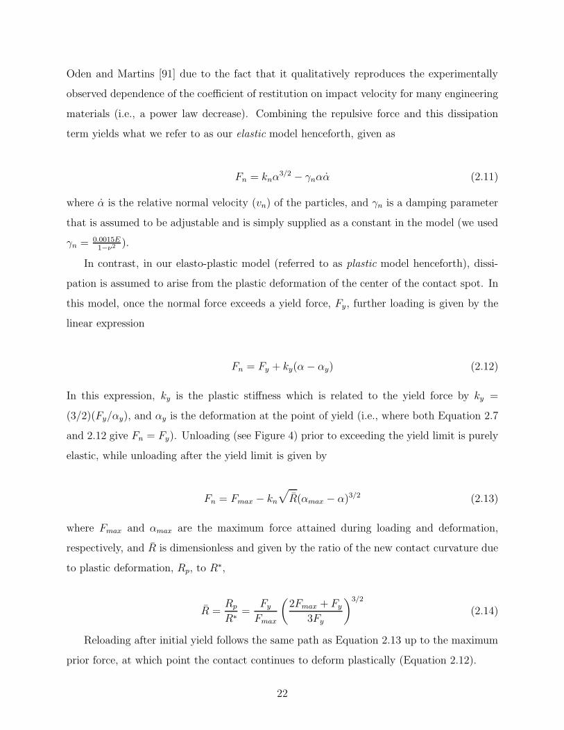
and 2.12 give Fn = Fy). Unloading (see Figure 4) prior to exceeding the yield limit is purely
elastic, while unloading after the yield limit is given by
Fn = Fmax − kn√
R(αmax − α)3/2 (2.13)
where Fmax and αmax are the maximum force attained during loading and deformation,
respectively, and R is dimensionless and given by the ratio of the new contact curvature due
to plastic deformation, Rp, to R∗,
R =Rp
R∗=
Fy
Fmax
(
2Fmax + Fy
3Fy
)3/2
(2.14)
Reloading after initial yield follows the same path as Equation 2.13 up to the maximum
prior force, at which point the contact continues to deform plastically (Equation 2.12).
22
α
F
yF
maxF
α αy max
yield point
load
ing
un
load
ing
Figure 4: Schematic showing force-displacement curve of elasto-plastic deformation for dry
particles.
While the yield force, Fy, can be loosely related to the yield stress (σy) of the bulk
material, in this work, we treat it in the same manner as γn from the spring-dashpot model.
2.2.2.2 Tangential Forces In our case, we used a simple “history dependent” tangential
force model which is very close to the model developed by Walton and Braun [73]. For each
time-step, the new tangential force acting at a particle-particle contact, Ft, is given as:
Ft = Fto − kt∆s (2.15)
where Fto is the old tangential force and kt∆s is the incremental change in the tangential
force during the present time-step due to relative particle motion; i.e., ∆s is the tangential
displacement during the present time-step. This displacement is calculated from the compo-
nent of velocity tangent to the contact surface, vt (i.e., ∆s = vtdt where dt is the time-step).
The tangential stiffness, kt, is not a constant and depends upon the overlap α :
kt(α) = 8G∗a = 8G∗√R∗α (2.16)
23
where a is the radius of the contact spot (=√R∗α) and G∗ is given by
1
G∗=
2− ν1G1
+2− ν2G2
(2.17)
where Gi is the shear modulus of the particle i. In this model, we must impose a discontinuity
in order to limit the tangential force to the Amonton’s law limit (Ft ≤ µfFn, where µf is
the coefficient of sliding friction).
Note that, there is no source of energy dissipation (prior to macroscopic sliding) in our
tangential force model, though it can be incorporated using a more involved model where kt
will assume different values depending upon loading, unloading and reloading [68, 100].
2.2.2.3 Comments on Rolling Friction As mentioned earlier in Section 2.2.1.3, we
do not consider any rolling friction. However, a small discussion on this contentious issue is
presented here for completeness. Rolling friction is a rarely employed force in mainstream
DEM simulations [101]. Nevertheless, there are two potential reasons for inclusion of such
a force when modeling real particles: to dissipate energy when particles roll on a smooth
surface, and to approximate the behavior of slightly aspherical particles. If rolling friction is
not considered, a spherical particle will continue to roll on a flat surface without stopping.
(As we have seen earlier, inter-particle forces act at the contact point between particles and
not at the mass center of a particle. This generates a torque and causes the particle to ro-
tate. The torque has contributions from two components of the tangential and asymmetrical
normal traction distributions (on the contact spot). In comparison with the contribution of
the tangential component, the determination of the contribution of the asymmetric normal
component, usually known as rolling friction torque, is very difficult and is still an active
area of research [88, 102–104]. The rolling friction torque is considered to be negligible in
many DEM models [82]. However, it has been shown that the torque plays a significant
role in some cases involving the transition between static and dynamic states, such as the
formation of shear band and heaping, and movement of a single particle on a plane [82].
24
2.2.3 Contact Detection Algorithm
Clearly, the necessity of a large number of particles coupled with small time-steps, makes
DEM a very computationally intensive technique. This situation can be exacerbated in
applications where multiple particle sizes or complex particle shapes are required. This
problem, however, can be partially overcome by the use of more effective contact detection
algorithms. However, contact detection itself can take up to 60% of the total CPU time in
some problems. Therefore, a current direction of research is to develop efficient algorithms
to minimize CPU time. There has been a considerable amount of research performed [3,
81, 105–124] on the topic of finding nearest neighbors and detection of contacts between
many bodies, both on spherical shapes and irregular shapes. Most of these algorithms can
be classified as body-based search or space-based search (alternatively, tree based search or
cell/bin based search). It is worth mentioning here that most of these search algorithms were
originated from general computing algorithms of computer science which were normally used
for traditional computing, computer graphics (CAD), animation, computational geometry,
collision detection and motion planning in robotics [125–129]. Now, we briefly review the
algorithm that we adopted for the present work along with its merits and demerits. We also
shed some light onto how the shortcomings of the algorithm employed here can be addressed.
Algorithms employing binary search (i.e., tree-based [129]) has a total contact detection
time which scales as T ∝ N ln(N) , where N is the total number of particles. Another body-
based search scheme which employs Delaunay triangulation [112] also has complexity varying
between O(N2) and O(N ln(N)). Some of these algorithms perform better for either loose or
dense packing. Table 1 shows different algorithms and their complexity. In this work, we use
the so-called No Binary Search (NBS) algorithm of Munjiza et al. [3], which is a cell based
algorithm. This algorithm is suitable for assembly of particles whose sizes are close to each
other and the total contact detection time scales as T ∝ N , which is a performance superior
to binary search algorithms. The NBS algorithm works well both for loose and dense packing
as it is independent of packing density. This is because the outer loop is always over the total
number of particles and not on the number of cells. If there is a particle size distribution, the
size of the cell is taken as the maximum diameter of the particle, and the algorithm becomes
25
somewhat less efficient owing to the fact that more contact checking within a cell is needed as
there can be many more particles in a cell (more than the optimum number of particles in a
cell). Therefore, NBS works well if dlarge/dsmall is small (close to 1.0) and if the mean number
of particles in a cell is 1.0 – 5.0 [121]. To overcome this difficulty for different sized particles
(polydispersity), very recently, some cell-based hierarchical search algorithms or multi-grid
search algorithms have been proposed [115, 120–122]. In this approach, depending upon
its size, a particle belongs to a layer of grids (or cells/bins) suitable for that size range.
Therefore, different layers of grids are possible and contact detection is performed in and
between different layers hierarchically.
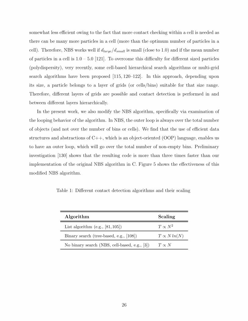
In the present work, we also modify the NBS algorithm, specifically via examination of
the looping behavior of the algorithm. In NBS, the outer loop is always over the total number
of objects (and not over the number of bins or cells). We find that the use of efficient data
structures and abstractions of C++, which is an object-oriented (OOP) language, enables us
to have an outer loop, which will go over the total number of non-empty bins. Preliminary
investigation [130] shows that the resulting code is more than three times faster than our
implementation of the original NBS algorithm in C. Figure 5 shows the effectiveness of this
modified NBS algorithm.
Table 1: Different contact detection algorithms and their scaling
Algorithm Scaling
List algorithm (e.g., [81, 105]) T ∝ N2
Binary search (tree-based, e.g., [108]) T ∝ N ln(N)
No binary search (NBS, cell-based, e.g., [3]) T ∝ N
26
0 10 20 30 40 50 60 70 80 90Total Number of Objects (N x 1000)
0
1
2
3
4
5
6
7
8
9
10C
onta
ct D
etec
tion
Tim
e (s
)Brute Force
NBS (Munjiza et al.)
NBS (present work)
Figure 5: Total contact detection time as a function of total number of particles. [◦] corre-sponds to our implementation of the original NBS algorithm of Munjiza et al. [3] in C and
[•] corresponds to the modification of the outer loop of the NBS algorithm using an efficient
data structure in C++. A naive brute force method where all particles are searched against
all other particles has also been included. Total contact detection time has been obtained
by running the outer loop 10 times in a 3.2 GHz, Intel Xeon processor.
27
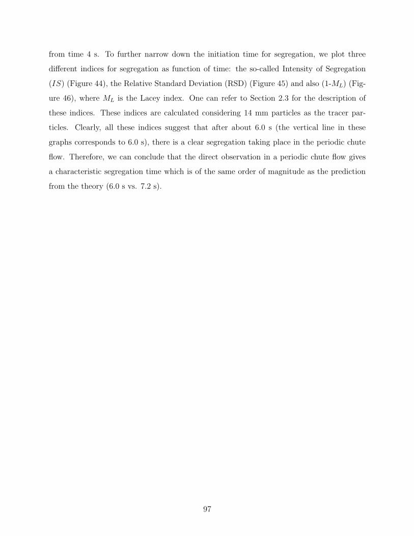
2.3 MIXING & SEGREGATION MEASURES
In this section, information about how to quantify mixing and segregation is presented. Fan
et al. [131] have described a number of mixing indices for various types of mixing situations
(such as in tumbler mixer, fluidized bed, etc.). A number of indices are used to quantify
the efficiency of mixing and this background information would be used to characterize the
systems described in the succeeding chapters. Merits and demerits of various mixing indices
have been examined by Rollins et al. [132]. Although (as noted by Fan et al. [131]) the
representation of the complex characteristics of a solids mixture via any available mixing
index appears to be far from satisfactory, in this work, we have employed multiple indices
to probe and ascertain the performance of a system.
Danckwerts [133] used the term “scale of scrutiny” as the maximum size of the segregating
regions that can cause the mixture to be considered acceptable for its intended use. For a
given powder, its quality of mixing decreases as the scale of scrutiny, with the extreme case
where each sample contains only one particle. In this section, some measures that attempt
to quantify the degree of mixing are described, among them Intensity of Segregation (IS),
which is the mixing measure frequently used in this work.
2.3.1 Intensity of Segregation
The Intensity of Segregation (IS) is essentially the standard deviation of the concentration
calculated at multiple locations in the granular bed, and is calculated using the following
expression:
IS = σ =
√
∑Nc
i=1(C − 〈C〉)2Nc − 1
(2.18)
where Nc is the number of concentration measurements, C is the concentration of the tracer
particles in the designated measurement location, and 〈C〉 is the average concentration of
that type of particle in the entire bed. It should be noted that large values (approaching 0.5
for a equi-volume mixture) of IS correspond to a segregated state while smaller values denote
more mixing. This particular index will be revisited in Section 3.3 when the experimental
procedure in a tumbler mixer will be discussed.
28
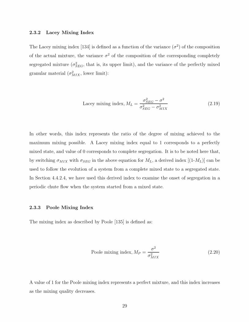
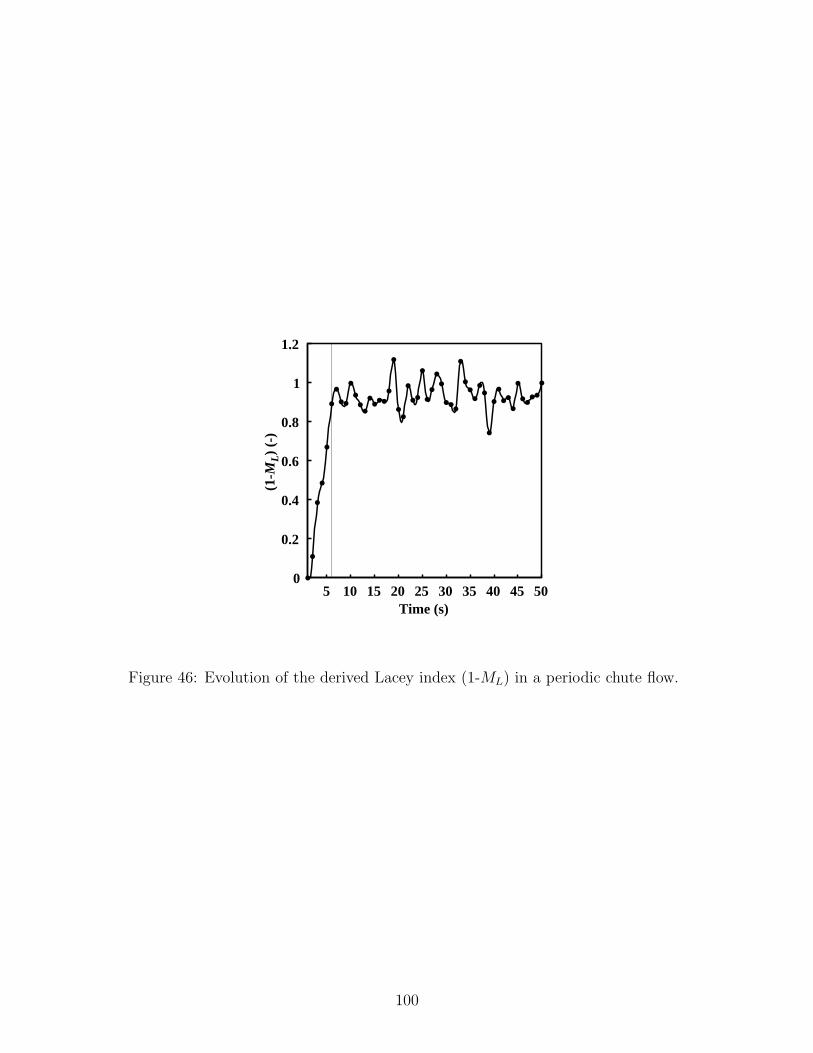
2.3.2 Lacey Mixing Index
The Lacey mixing index [134] is defined as a function of the variance (σ2) of the composition
of the actual mixture, the variance σ2 of the composition of the corresponding completely
segregated mixture (σ2SEG, that is, its upper limit), and the variance of the perfectly mixed
granular material (σ2MIX , lower limit):
Lacey mixing index,ML =σ2SEG − σ2
σ2SEG − σ2
MIX
(2.19)
In other words, this index represents the ratio of the degree of mixing achieved to the
maximum mixing possible. A Lacey mixing index equal to 1 corresponds to a perfectly
mixed state, and value of 0 corresponds to complete segregation. It is to be noted here that,
by switching σMIX with σSEG in the above equation for ML, a derived index [(1-ML)] can be
used to follow the evolution of a system from a complete mixed state to a segregated state.
In Section 4.4.2.4, we have used this derived index to examine the onset of segregation in a
periodic chute flow when the system started from a mixed state.
2.3.3 Poole Mixing Index
The mixing index as described by Poole [135] is defined as:
Poole mixing index,MP =σ2
σ2MIX
(2.20)
A value of 1 for the Poole mixing index represents a perfect mixture, and this index increases
as the mixing quality decreases.
29
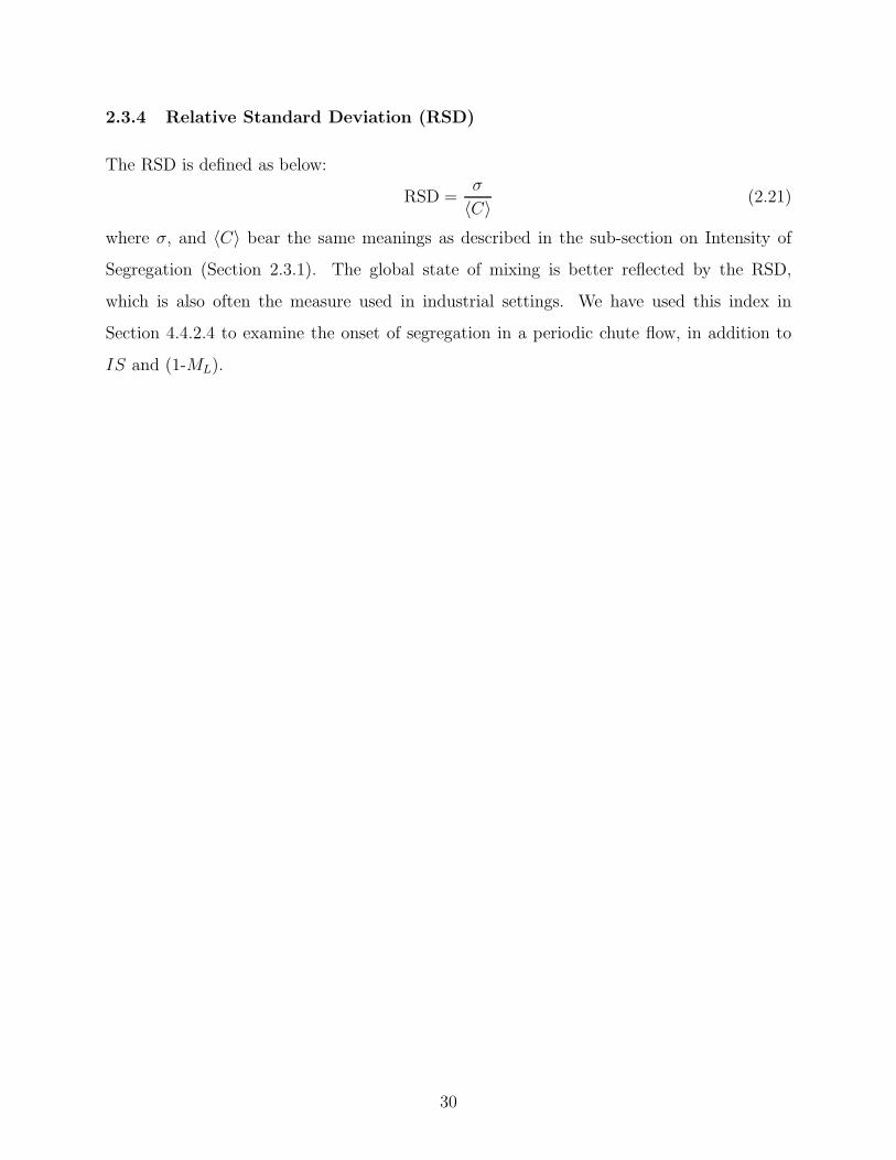
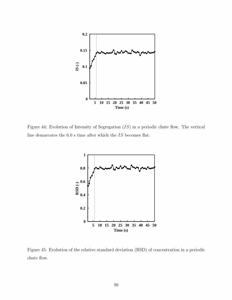
2.3.4 Relative Standard Deviation (RSD)
The RSD is defined as below:
RSD =σ
〈C〉 (2.21)
where σ, and 〈C〉 bear the same meanings as described in the sub-section on Intensity of
Segregation (Section 2.3.1). The global state of mixing is better reflected by the RSD,
which is also often the measure used in industrial settings. We have used this index in
Section 4.4.2.4 to examine the onset of segregation in a periodic chute flow, in addition to
IS and (1-ML).
30
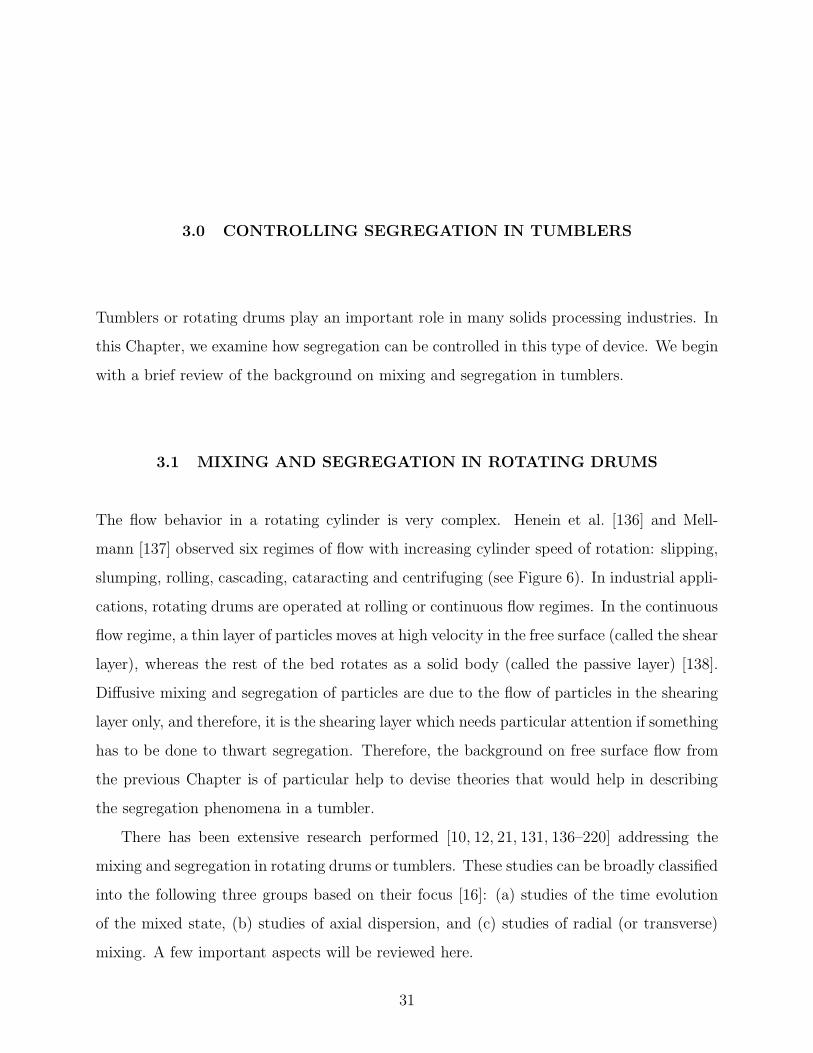
3.0 CONTROLLING SEGREGATION IN TUMBLERS
Tumblers or rotating drums play an important role in many solids processing industries. In
this Chapter, we examine how segregation can be controlled in this type of device. We begin
with a brief review of the background on mixing and segregation in tumblers.
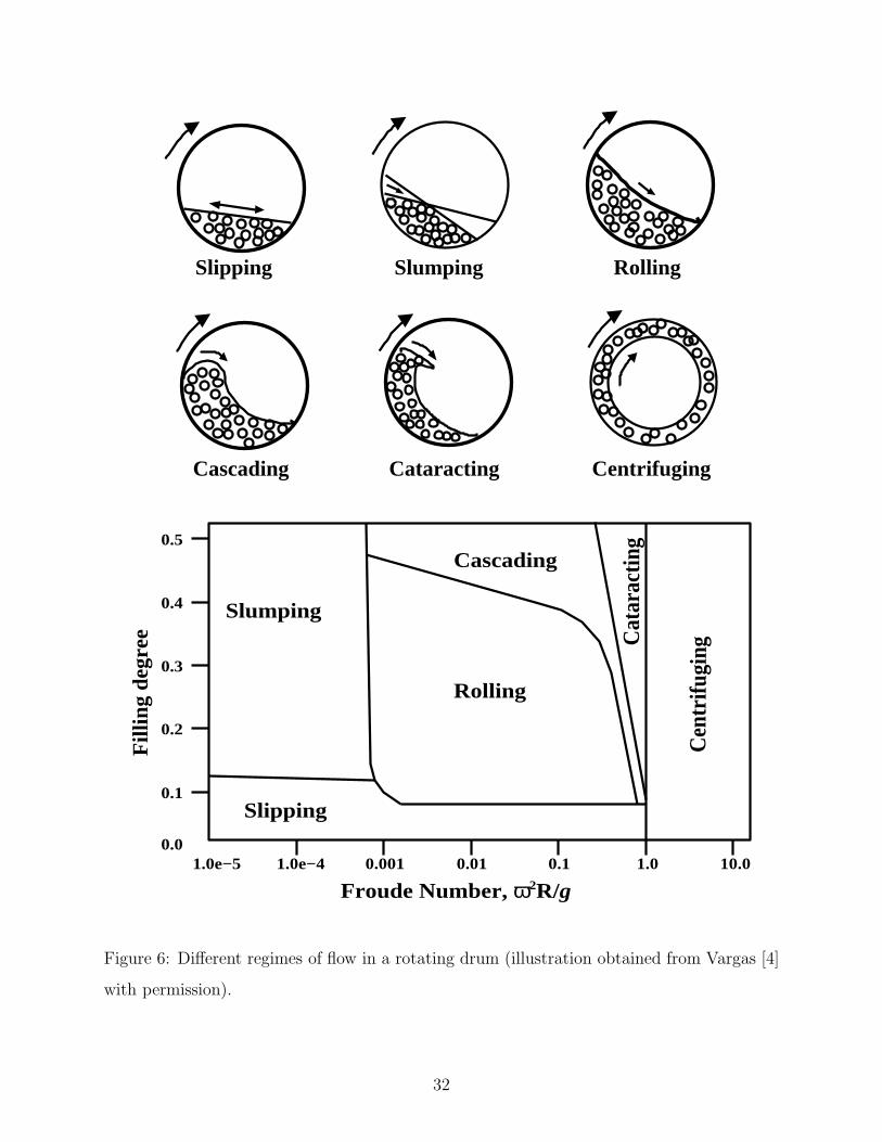
3.1 MIXING AND SEGREGATION IN ROTATING DRUMS
The flow behavior in a rotating cylinder is very complex. Henein et al. [136] and Mell-
mann [137] observed six regimes of flow with increasing cylinder speed of rotation: slipping,
slumping, rolling, cascading, cataracting and centrifuging (see Figure 6). In industrial appli-
cations, rotating drums are operated at rolling or continuous flow regimes. In the continuous
flow regime, a thin layer of particles moves at high velocity in the free surface (called the shear
layer), whereas the rest of the bed rotates as a solid body (called the passive layer) [138].
Diffusive mixing and segregation of particles are due to the flow of particles in the shearing
layer only, and therefore, it is the shearing layer which needs particular attention if something
has to be done to thwart segregation. Therefore, the background on free surface flow from
the previous Chapter is of particular help to devise theories that would help in describing
the segregation phenomena in a tumbler.
There has been extensive research performed [10, 12, 21, 131, 136–220] addressing the
mixing and segregation in rotating drums or tumblers. These studies can be broadly classified
into the following three groups based on their focus [16]: (a) studies of the time evolution
of the mixed state, (b) studies of axial dispersion, and (c) studies of radial (or transverse)
mixing. A few important aspects will be reviewed here.
31
Slipping Slumping Rolling
Cascading Cataracting Centrifuging
0.0
0.1
0.2
0.3
0.4
0.5
1.0e−5 1.0e−4 0.001 0.01 0.1 1.0 10.0
Slumping
Slipping
Rolling
Cascading
Cat
arac
ting
Cen
trifu
ging
Froude Number, ω2R/g
Fill
ing
degr
ee
Figure 6: Different regimes of flow in a rotating drum (illustration obtained from Vargas [4]
with permission).
32
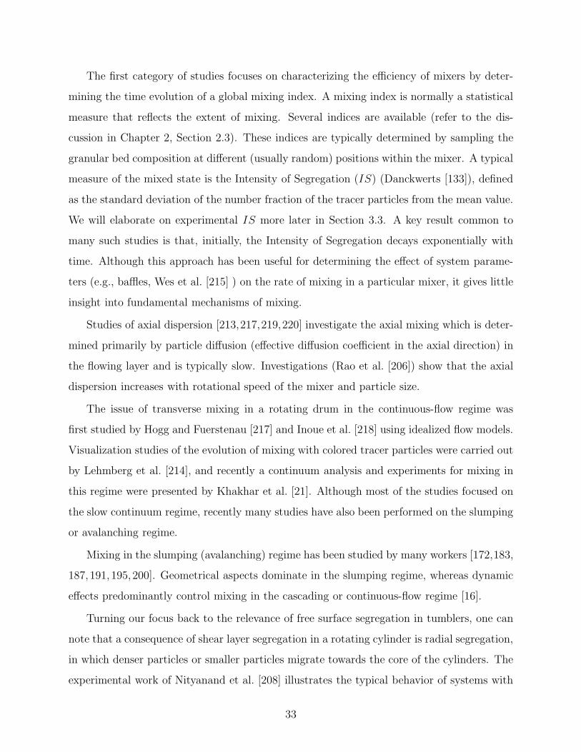
The first category of studies focuses on characterizing the efficiency of mixers by deter-
mining the time evolution of a global mixing index. A mixing index is normally a statistical
measure that reflects the extent of mixing. Several indices are available (refer to the dis-
cussion in Chapter 2, Section 2.3). These indices are typically determined by sampling the
granular bed composition at different (usually random) positions within the mixer. A typical
measure of the mixed state is the Intensity of Segregation (IS) (Danckwerts [133]), defined
as the standard deviation of the number fraction of the tracer particles from the mean value.
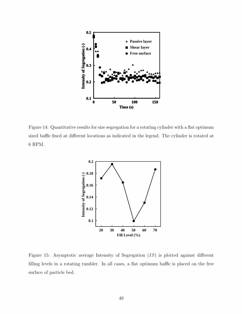
We will elaborate on experimental IS more later in Section 3.3. A key result common to
many such studies is that, initially, the Intensity of Segregation decays exponentially with
time. Although this approach has been useful for determining the effect of system parame-
ters (e.g., baffles, Wes et al. [215] ) on the rate of mixing in a particular mixer, it gives little
insight into fundamental mechanisms of mixing.
Studies of axial dispersion [213,217,219,220] investigate the axial mixing which is deter-
mined primarily by particle diffusion (effective diffusion coefficient in the axial direction) in
the flowing layer and is typically slow. Investigations (Rao et al. [206]) show that the axial
dispersion increases with rotational speed of the mixer and particle size.
The issue of transverse mixing in a rotating drum in the continuous-flow regime was
first studied by Hogg and Fuerstenau [217] and Inoue et al. [218] using idealized flow models.
Visualization studies of the evolution of mixing with colored tracer particles were carried out
by Lehmberg et al. [214], and recently a continuum analysis and experiments for mixing in
this regime were presented by Khakhar et al. [21]. Although most of the studies focused on
the slow continuum regime, recently many studies have also been performed on the slumping
or avalanching regime.
Mixing in the slumping (avalanching) regime has been studied by many workers [172,183,
187, 191, 195, 200]. Geometrical aspects dominate in the slumping regime, whereas dynamic
effects predominantly control mixing in the cascading or continuous-flow regime [16].
Turning our focus back to the relevance of free surface segregation in tumblers, one can
note that a consequence of shear layer segregation in a rotating cylinder is radial segregation,
in which denser particles or smaller particles migrate towards the core of the cylinders. The
experimental work of Nityanand et al. [208] illustrates the typical behavior of systems with
33
size segregation. Percolation dominates at low rotation rate (RPM) of the cylinder and
the smaller particles sink to lower levels in the flowing layer and thus form a core at the
centre. However, at higher rotational speeds, the segregation pattern reverses, with the
smaller particles at the periphery instead of the core. These results reflect the challenge of
the segregation processes in the shearing layer.
Recent studies of radial segregation have focused primarily on the dynamics and extent
of segregation in the low-rotational-speed regime [16]. 2D DEM simulations were used to
study the density segregation [204] and size segregation [194] in the rolling regime. Size
segregation in two dimensions has been reported by Clement et al. [199] in the avalanching
regime and by Cantelaube and Bideau [198] in the rolling regime experimentally. Smaller
particles formed the central core in both these experiments. Cantelaube and Bideau also
reported the statistics of trapping of the small particles at different points in the layer.
Baumann et al. [201] suggested a similar trapping mechanism for size segregation based on
computations using a 2D heaping algorithm, and Prigozhin and Kalman [188] proposed a
method for estimating radial segregation based on measurements taken in heap formation.
Khakhar et al. [21] have reported experiments and theory of density segregation. They
proposed a constitutive model for the segregation flux in cascading layers and validated the
model by both particle dynamics and Monte Carlo simulations for steady flow down an
inclined plane. Earlier, Alonzos et al. [205] showed how an optimum combination of size and
density differences can be used to minimize segregation.
Very recently, Gui et al. [141] studied the microscopic and macroscopic characteristics of
mixing based on fractal dimension analysis and Shannon entropy analysis, respectively. They
found, by numerical analysis on the dimension of the fractal interface, that a slow rotational
speed is favorable for particle mixing. Recent DEM studies on unbaffled tumblers by Arntz
et al. [143] concentrated on the effect of drum rotational speed and fill level on mixing. They
studied many regimes such as rolling, cascading, cataracting and centrifuging. Their studies
indicate that good mixing is possible for Froude Numbers in the range 0.25<Fr<0.68. Also,
high fill fractions (>65%) show the most intense segregation, which is at variance with the
earlier prediction by Dury and Ristow [221]. It is well established that mixing and segregation
34
patterns are sensitive to the container geometry and fill level [152,185,197]. The dynamics of
mixing and segregation are still not well understood, and therefore, all the designs of solids
mixers currently are empirical. Several approaches have been proposed to control or eliminate
segregation. McCarthy et al. [197] found that the mixing is enhanced in the avalanching
regime for an odd number of baffles. Wightman and Muzzio [212] performed experiments
for size segregation in a drum, both for pure rotation and rotation with vertical rocking.
They found that rocking accelerates axial mixing. Samadani and Kudrolli [176] found that
segregation could be reduced by adding a small volume fraction of fluid. Recently, Li and
McCarthy [160] found that segregation could be turned on or off by adding small amounts
of moisture in multi-sized mixture with particles having different surface characteristics.
Hajra and Khakhar [161] found that segregation could be eliminated by using a small (in
comparison to the diameter of the cylinder) rotating impeller placed at the axis of rotation,
that is, in the flowing layer. Jain et al. [153], Thomas [177] and Hajra and Khakhar [222]
performed experiments for binary mixtures composed of different size and different density
particles and they found that mixing can occur instead of segregation if the denser beads
are bigger, and also if the ratio of particle size is greater than the ratio of particle density.
Khakhar and Ottino [223] have summarized the findings of many studies of granular flow
in tumblers so that they can be applied to the design and scale up for problems of industrial
importance. For summaries of recent work on mixing and segregation in tumblers, one can
refer to Duran [224] or Ristow [225].
One can observe that the solutions to combat segregation based on the past studies can be
categorized into two groups: Change the particles or change the process [226]. Changing the
particles may involve controlling inter-particle adhesion or balancing the differences in size
and density. Changing the process may involve geometrical changes (such as manipulating
baffles) or operational changes (such as varying the tumbler rotational speed). Looking back
at the developments on the design of baffles for rotating cylinders, we find that very little
is known from a theoretical point of view on the effect of baffles on solid mixing, even in
simple cases limited to monodispersed systems. Industries use empirical designs based on
35
past experience, which often have no theoretical basis. Moreover, a literature search yields
no previous studies dealing with issues involving novel baffle shapes and their placements in
a solid mixer and how their designs will affect segregation.
Recently, Shi et al. [31], have shown that periodic flow inversions either manually – in
a chute – or via selective baffle placement in a tumbler-type mixer – can serve as a generic
method for eliminating segregation in free-surface flows, perhaps the most common and
well-studied of granular flows [39, 75, 227].
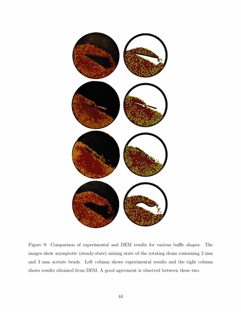
In this work, for the first time, we use experiments and simulations to study the effects
of various design and operating parameters, such as baffle shape and placement, on mixing
of binary mixtures with different sizes or densities. We show that periodic flow inversion
can be used to reduce segregation in a rotating cylinder, where different baffle shapes and
placements were engineered based on the hypothesis of flow modulation, and some of these
novel designs yielded excellent mixing results in actual experiments. Attempts are made to
link this technique to the probability distribution of the number of times a particle passes
through the flowing layer per rotation of the drum, and using this information, predictions
are made as to which baffle configurations would produce better mixing. In order to achieve
this objective, the numerical experimental tool DEM (Discrete Element Method) has been
extensively used in the present study.
In the next section, we take a brief look at the hypothesis of flow modulation as mentioned
above. Mathematical expressions describing the hypothesis in a tumbler are also presented.
This is expected to aid in designing actual or numerical experiments to corroborate the
hypothesis, either directly or indirectly.
3.2 HYPOTHESIS: TIME MODULATION IN A TUMBLER
Time-modulation in fluid mixing and other dynamical systems [24] is a fairly common prac-
tice, but has found only limited applications in granular processing [197,228,229]. As already
mentioned in Section 3.1, Shi et al. [31] have shown that periodic flow inversions via selective
baffle placement can serve as a generic method to thwart segregation. The key to adapting
36
this idea to free-surface segregation lies in recognizing two important facts: that it takes
a finite time for material to segregate and that there is always a preferred direction that
particles tend to segregate. For example, in a free-surface flow, small particles need time to
percolate through the flowing layer (also, smaller particles travel faster than the larger par-
ticles [230]); thus, if the flow is interrupted before the small particles could reach the bottom
of the flowing layer, segregation can be prevented. This relatively simple observation can be
employed to engineer systems that counteract segregation.
In order to capitalize on the fact that this flow interruption can thwart segregation, one
next needs to invert the flowing layer, prior to reinitiating the flow. One way to achieve
this two-step process in a continuous flow is to invert the flowing layer at a sufficiently high
frequency, fcrit, fcrit > t−1S , where tS is the characteristic segregation time. A critical issue
with this technique is that a full understanding of segregation kinetics – and therefore, the
characteristic segregation time, tS – is still lacking. However, this hypothesis can well be
tested indirectly for many baffle configurations in a rotating tumbler or directly in a chute
flow segregation tester (Chapter 4) using scaling arguments and utilizing existing theoretical
tools [21, 30].
Now we attempt to derive an expression for critical forcing frequency in an unbaffled
tumbler owing to its simplicity as a model system. As a closed-form expression of the
critical forcing frequency for baffled tumbler is not available at present due to the inherent
complexity of the flow, the hypothesis of time modulation can be translated into some other
indirect measure (like the number of layer passes a particle makes) to implement it in a baffled
tumbler and to apply this knowledge in understanding the behavior of baffled tumblers. In
fact, one of the objectives of this present work is to take up this challenge and apply this
hypothesis to explain the behavior of baffled tumblers.
For size segregation, the segregation velocity takes the form vS = KT (1− d)+fKS(1− d)
[21], where (1− d) is the dimensionless particle size difference, f is the number fraction of the
segregating species, KS and KT are segregation constants, which depend on the local number
density ratio, local void fraction and granular temperature, respectively. For an unbaffled
tumbler, the characteristic segregation time may then be written as tS = δo/[KT (1 − d) +
fKS(1 − d)], where δo is the maximum shear layer thickness and also corresponds to the
37
characteristic length for segregation. The expression for tS above can also be recast as
tS = δo/[ξ(1− d)], where ξ = (KT +fKS). Again, due to current theoretical uncertainty and
the time-varying nature of our flow (as well as our granular temperature, pressure, etc.), ξ
is treated as a fitting parameter that is a function of the local number density, the granular
temperature and the composition of the mixture [21]. Referring to the work by Khakhar et
al. [223], the thickness of the shear layer at the midpoint is given by δo/R = (ω/γo)1/2, such
that the time for size segregation can be written as
tS =
(
ω
γo
)1/2R
ξ(1− d)(3.1)
where, γo is the shear rate at midpoint of the layer and is given by
γo =
[
g sin(βm − βs)
cd cos(βs)
]1/2
(3.2)
The parameter c in Equation 3.2 is the dimensionless collisional viscosity and it is ap-
proximately constant with a value of ≈ 1.5 for all Froude numbers Fr = ω2R/g and size
ratios s = d/R [223]. βs and βm are the static and dynamic angles of repose, respectively.
The critical perturbation frequency, fcrit is then given by
fcrit =1
tS=
(
γoω
)1/2(1− d)ξ
R(3.3)
In order to suppress segregation in an unbaffled tumbler, a forcing frequency should be
chosen such that the mean residence time of the particles in the layer τmean = 2π/√ωγ [155]
is less than the time of segregation tS. The effective forcing frequency is then given by,
fe =1
τmean=
√ωγo2π
(3.4)
and the ratio of frequencies (using Equations 3.3 and 3.4) is given by
fefcrit
=ωR
2π(1− d)ξ=
γoδ2o
2πR(1− d)ξ(3.5)
A similar procedure can be crafted for density segregation [144], resulting in an expression
for the frequency ratio of the form
38
fefcrit
=ωR
2π(1− ρ)KS=
γoδ2o
2πR(1− ρ)KS(3.6)
where (1 − ρ) is the dimensionless density difference and KS is a segregation constant that
depends on local void fraction and granular temperature.
The fact that all the relations used in developing the frequency ratios above are based
on data for monodispersed system and for unbaffled tumblers, might render our analysis
somewhat limited for application in the baffled cases. Nevertheless, as we mentioned earlier,
we show that this general theory can still be applied indirectly to explain the behavior of
baffled tumblers.
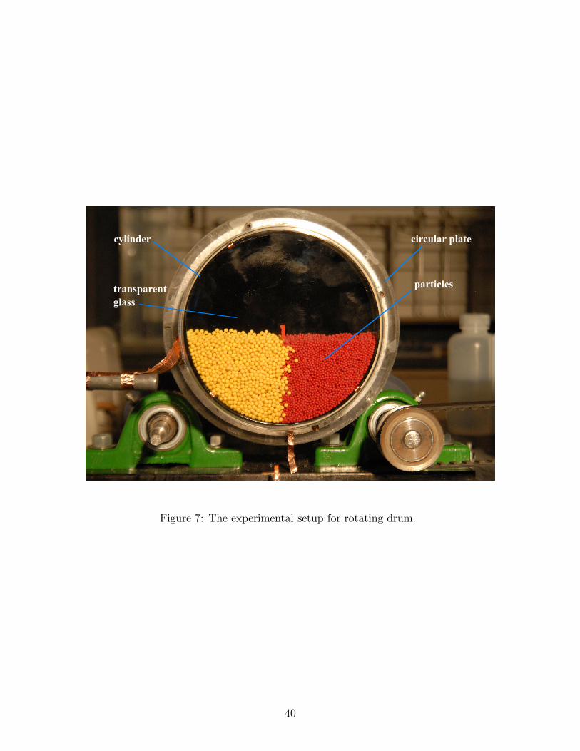
3.3 EXPERIMENTS
Experiments are carried out in a quasi-2D rotating cylinder (1.5 cm in length and 13.8 cm
in diameter), which is mounted on a circular plate attached to a bigger rotating drum (see
Figure 7 for the setup). The bigger drum is rotated using a computer controlled stepper
motor at a fixed rate (6 RPM). The cylinder is made up of two sets of transparent glass discs,
which is fitted face to face to close the cylinder. This arrangement also helps in dispensing
particles when a particular experiment is completed. We used nearly spherical cellulose
acetate beads as the model particles. We mainly focus on size segregation experiments and
binary mixtures (equal volume, 50:50 v/v) composed of 2 mm and 3 mm acetate beads are
used.
In a typical experimental run, particles are placed in the cylinder using a divider so
that the initial particle bed remains completely segregated (see Figure 7 or Figure 8). All
experiments are carried out using 50% cylinder fill fraction. A digital camera (Nikon D200)
with a resolution of 6 Mega pixels is used to capture the photographs as the experiment
progresses and the evolution of the system from a complete segregated state to a mixing state
is observed. Digitized images are also taken at low shutter speeds in a separate experiment
to calculate the shearing or flowing layer thickness (δ0) at the layer mid point [231] when no
baffle was used. Photographs are captured at every half cylinder rotation. An image analysis
39
circular platecylinder
particlestransparent
glass
Figure 7: The experimental setup for rotating drum.
40
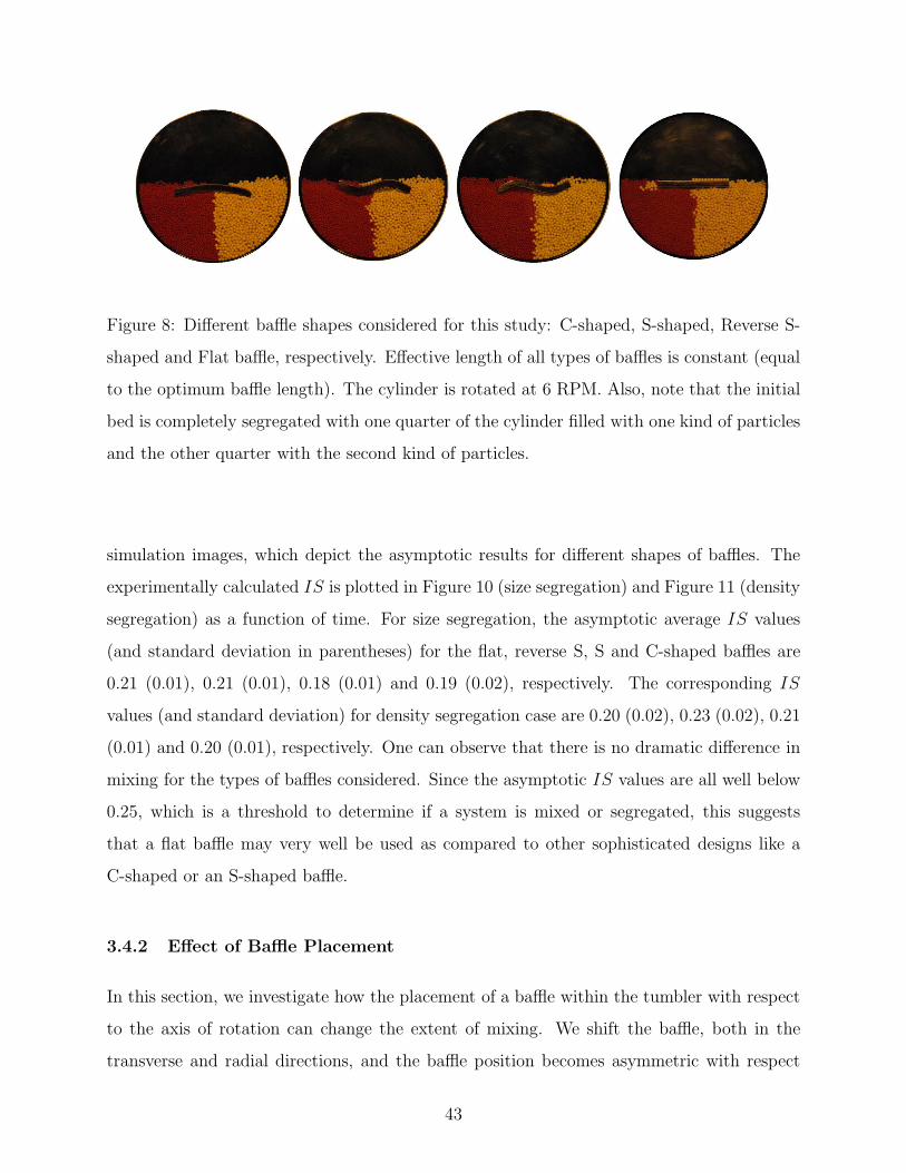
technique, which relies on the colors of the particles to identify different sized particles, is
used to compute the distribution of particles as a function of time. This procedure yields
the information required to calculate the Intensity of Segregation (IS) (refer to Section 2.3)
using Equation 2.18 for each experimental run.
With regards to the quantification of mixing, it is important to measure the extent of
mixing in order to investigate the performance of a mixer. As discussed in Section 2.3,
several methods of mixing measures are available in the literature. Among them, mixing
index [158] or Intensity of Segregation [133] are most commonly used. In this study, we
have used the Intensity of Segregation (IS) as the method of measurement of mixedness.
Low IS means good mixing. The captured images from experiments are divided into Nc
number of uniformly distributed boxes or cells and the concentration C at the center of a
cell is calculated from the fraction of particles with a specific color (denoting a specific-sized
particle) [21] in that cell. The mean value of the concentration, < C >, of a particular
species is the average concentration of all the cells. Also, as the IS is plotted over time as
the mixing process evolves, the asymptotic state is defined as the number of revolutions after
which the Intensity of Segregation becomes flat.
Both the DEM simulations and the experiments use cellulose acetate particles in thin
(≈ 6-7 particle deep) and ≈ 40-60 particle wide tumblers. The simulated particle sizes and
densities (as well as vessel size) are matched to their corresponding experiments as closely
as possible; however, the particle stiffness and other parameters used have been reduced in
order to decrease necessary simulation time (a practice shown to have essentially no impact
on flow kinematics [232]) in some simulations (using so-called “soft” particles). Table 2
lists the material properties used in the simulations. Note that an elasto-plastic model with
actual material properties is used when the objective is to compare simulation results with
the experimental data. On the other hand, fictitious “soft” material properties are used
for performing other studies (e.g., effect of number of baffles, etc.) when comparison with
experimental data is not the primary aim.
41
Table 2: Material properties used in the simulations
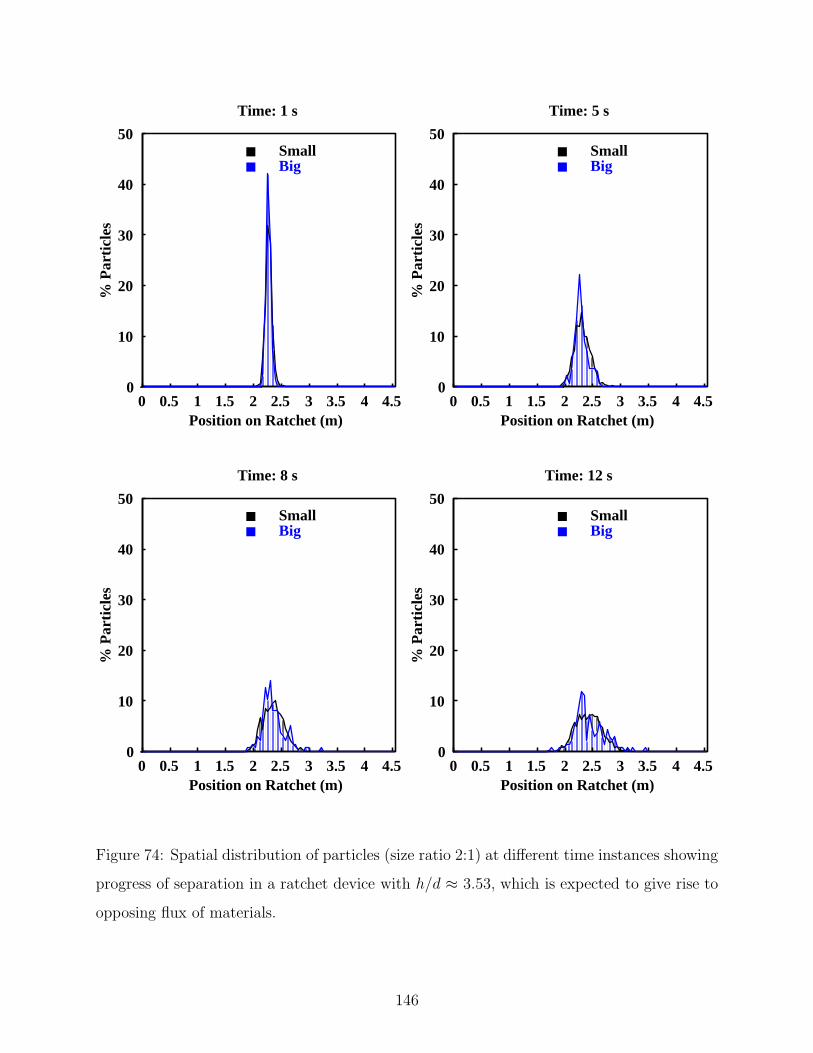
Figure 74: Spatial distribution of particles (size ratio 2:1) at different time instances showing
progress of separation in a ratchet device with h/d ≈ 3.53, which is expected to give rise to
opposing flux of materials.
146
6.0 SUMMARY AND OUTLOOK
In this chapter, a brief summary of the major contributions of the current work is presented
along with an outlook on future extensions. A short discussion on the many challenges to
link the fundamental physics of particle flow and the current industrial needs is also included
here.
6.1 CONTROLLING SEGREGATION IN TUMBLERS
Segregation in granular materials has been studied for a long time but its theoretical under-
standing even in the most simple cases is yet not complete. When particles differ in almost
any mechanical property, a small agitation leads to flow induced segregation. Controlling
or minimizing segregation continues to be a complicated problem. Industries use empirical
designs based on the past experiences, which often have no theoretical basis. A literature
search yields no previous studies dealing with issues involving novel baffle shapes and their
placements in a solids mixer and how their designs will affect mixing and segregation. In this
work, for the first time, we use experiments and simulations to study the effects of various
design parameters, such as baffle shapes and placement, on the mixing of binary mixtures
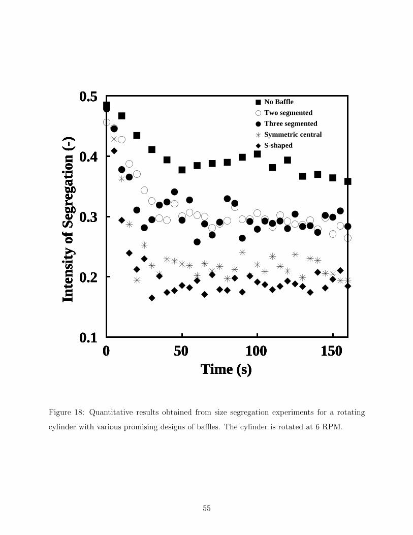
with different sizes or densities. It has been demonstrated that segregation in a rotating
drum can be dramatically reduced by introducing periodic flow inversions within the drum
by employing novel baffle designs. Both experimental observations and simulation results
agree qualitatively and the simulation tool is further used to test our hypothesis, which states
that the time modulation in the shearing layer is the key to thwarting segregation.
147
Segregation can be minimized if the particle flow is inverted at a rate above a critical
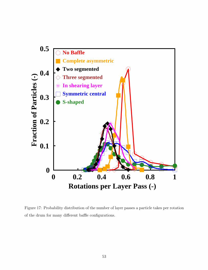
forcing frequency. For a rotating drum, this translates to the probability distribution of
the number of times a particle passes through the flowing layer per rotation of the drum.
A broader probability distribution signifies that the orientation of a particle will become
essentially uncorrelated to its previous orientation. Therefore, the baffle designs that produce
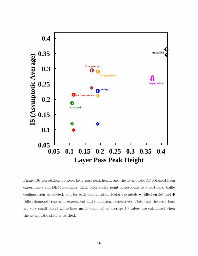
a broader distribution are expected to yield better mixing results. It has been shown that the
peak height of the layer pass distribution correlates strongly with the experimentally obtained
intensity of segregation. This observation actually demonstrates that the hypothesis of flow
inversion can be used for designing new baffles and examining the effectiveness of a new
design. Moreover, the characterization tool (layer-pass simulations) that is developed to test
the hypothesis can easily be used to examine different baffle configurations and predict their
performances.
As noted by Khakhar et al. [223], the time is ripe to exploit the knowledge gained
about surface flows and to apply it to design and scale-up solids processing devices. In this
spirit, the current work has attempted to test the hypothesis regarding a critical forcing
frequency (flow inversion) to mitigate segregation. The hypothesis has been embodied in
a mathematical form by utilizing the existing knowledge (continuum-derived) developed by
other researchers, and is used as an elimination tool to select optimum designs of tumbler
mixers from a host of promising baffle designs.
6.2 SEGREGATION IN A CHUTE FLOW
Granular materials are omnipresent. Many man-made or natural processes involve flow of
granular materials. Industrial applications typically involve handling and processing of a
large amount of multi-sized granular materials, which may have different shapes and densi-
ties. These processes require many solids handling devices like hopper, chute, etc. In this
work, a simple chute flow consisting of both mono-sized and polydisperse spherical granular
particles is analyzed. Effects of various parameters like charge amount, particle size, falling
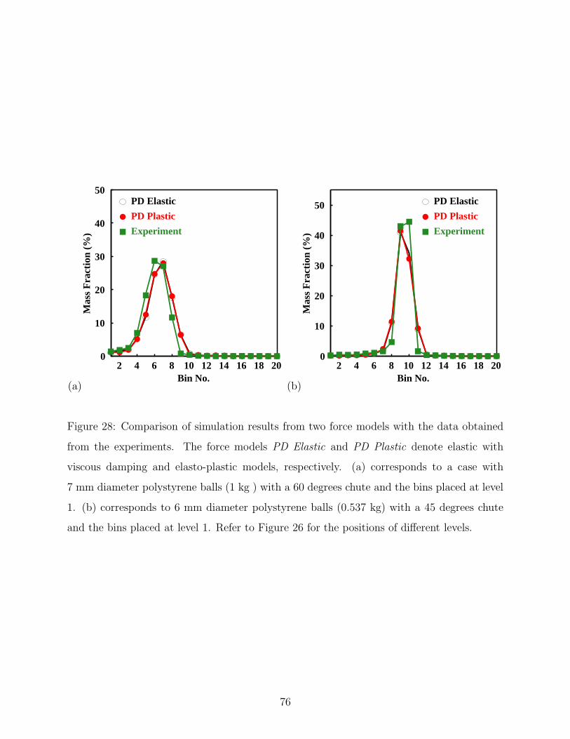
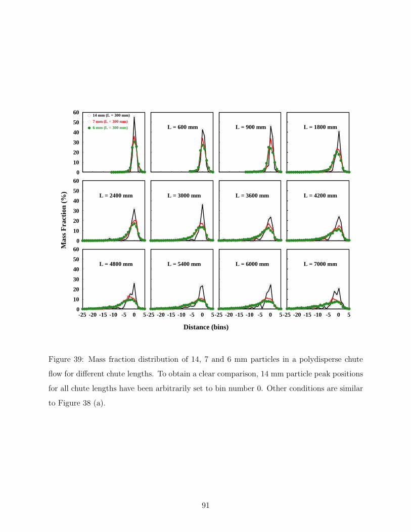
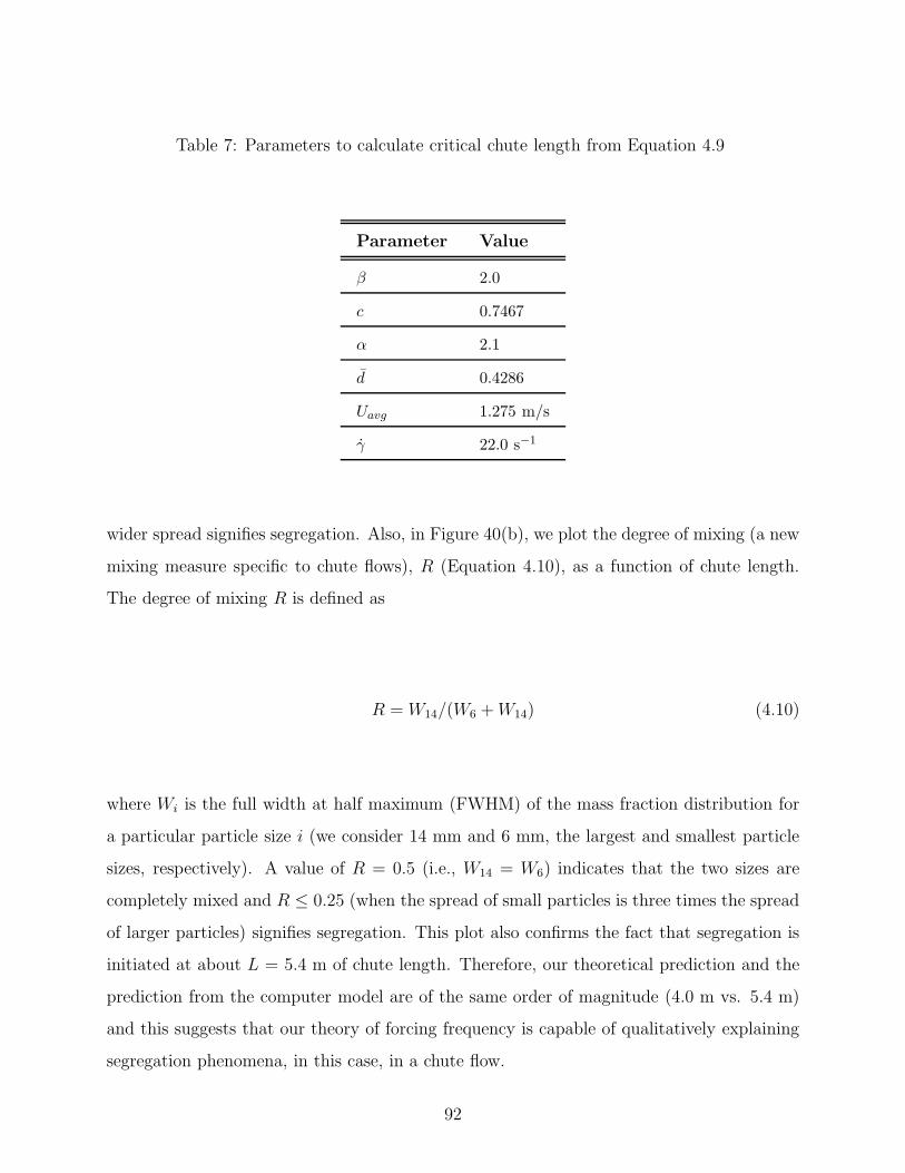
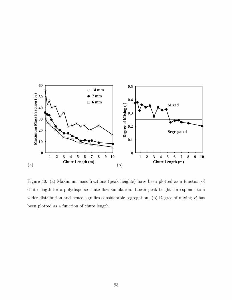
height and chute angle are studied systematically to examine how the mass fraction distri-
148
bution in the trajectories are affected by these parameters. A contact force parameter of the
DEM model has been adjusted in order to obtain reliable results and account for the devia-
tion from experimental observations. The tuned model is then used to find the critical chute
length for segregation as per our hypothesis regarding a critical forcing frequency. Both a
finite length chute and a periodic chute are used to test the hypothesis beyond doubt.
In the present investigation, we are only concerned about the mass fraction distribution of
particles in the bins placed below the chute. However, there are many applications where the
distribution of porosity or voidage of the bed is of utmost importance (like in a blast furnace
or in many fluidized beds where a gas has to pass through the particle bed). Therefore, the
present work can be extended to calculate the porosity or voidage of the particle bed after
deposition and the effects of many parameters on that. With regards to the significance and
practical applications of the results described in this part of the work, it is sufficient to say
that a reliable model can be used to design and probe any granular flow system employing a
chute for transfer of materials. And, there are plenty of industrial applications where these
investigations would help in improving productivity and product quality.
6.3 RATE-BASED SEPARATION IN COLLISIONAL FLOWS
While segregation is often an undesired effect, sometimes separating the components of a
particle mixture is the ultimate goal in many industrial processes. Rate-based separation
processes hold promise as both green and less energy intensive, when compared to conven-
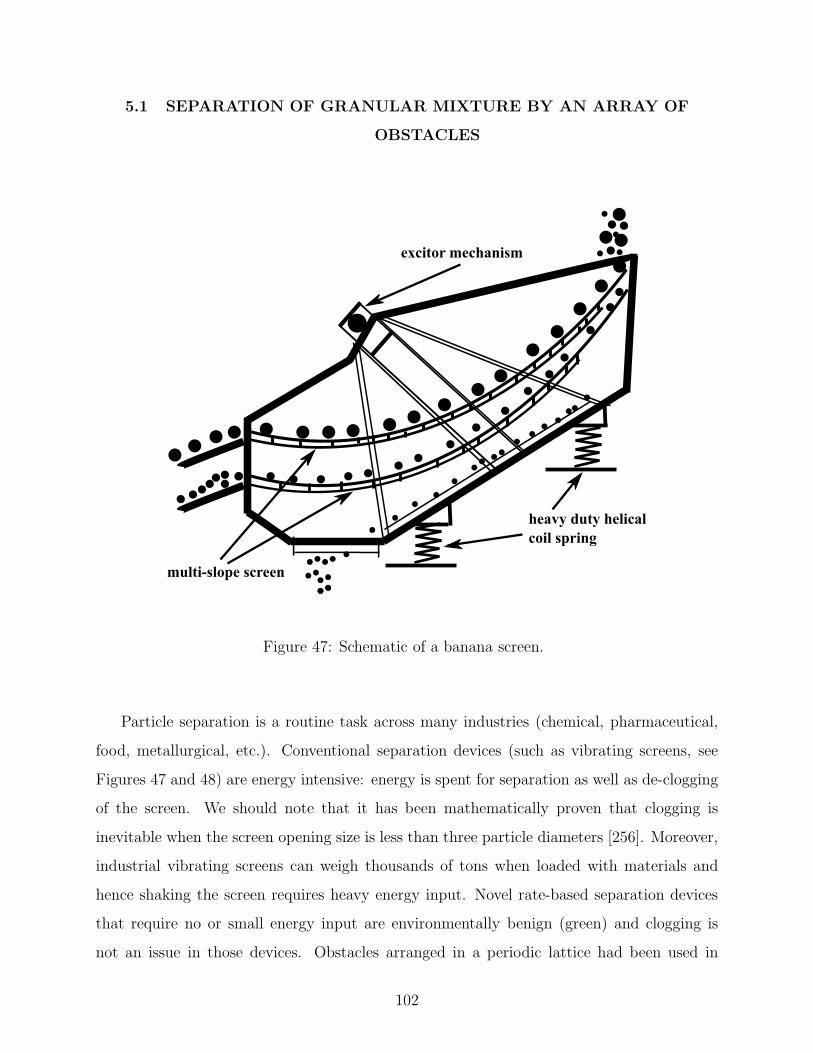
tional particle separations technologies such as vibrating screens or flotation methods.
It has been demonstrated, for the first time, that a device inducing diffusive motion to
the constituents of a mixture by way of gravity-driven collisional flow through an array of
obstacles can be used to separate particles effectively, without any external energy input.
The effects of various design and operating parameters on the extent or quality of separation
are investigated by means of a simple single particle model (based on a random walk theory)
along with experiments and DEM simulations. It has been found that the ratio of the particle
size to the available gap between two obstacles (called effective diameter or deff) is a key
149
parameter controlling the separation. This parameter is also a measure of the probability
of a particle colliding with a peg. Smaller particles are found to be faster (lower deff ,
and hence, relatively fewer number of collisions) than the larger ones, in both simulations
and experiments. Also, the extent of separation deteriorates as the loading of the device is
increased due to relatively high number of dissipative collisions for all types of particles, which
effectively reduce their relative mobility (in the extreme case, jamming occurs). Realization
of a complete theoretical model to predict the length (L) or time (t) required for obtaining
a desired extent of separation in a particular device with a given design and operating
parameter is still elusive and could be the topic of future research.
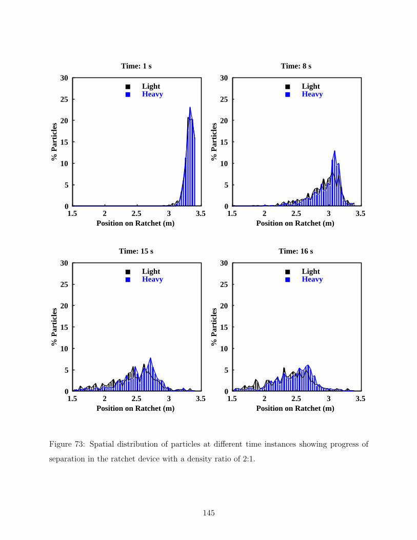
In another example of a novel separation technique, it has been demonstrated that a
ratchet mechanism employing a vibrating saw-toothed base can be used to induce different
mobility for different types of particles. A directed current of particle is produced perpen-
dicular to the energy input. In contrast to the collisional separation device considered in
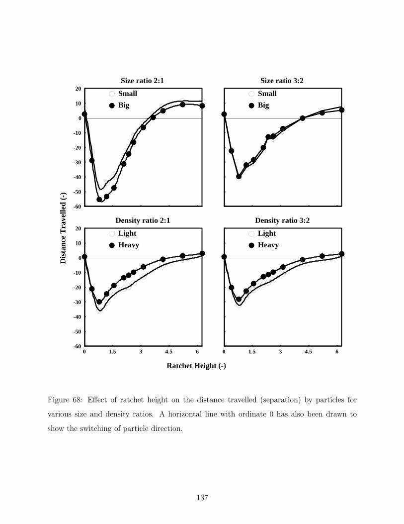
Section 5.1 where smaller particles travel faster, the larger or lighter particles in general
move faster in a ratchet device. Therefore, it is shown that the final goal of separation
can be achieved by means of different opposing mechanisms or exploiting phenomena which
might seem to be at odds when compared in a general sense. It has been demonstrated and
confirmed in this study that a ratchet can be used to separate particles, but the quality
of separation is not as good as a gravity-driven collisional separation device. Also, a com-
plete theoretical or a mathematical description of the process relating different design and
operating parameters in the device still remains an open question owing to the complexity
of the process, which is characteristic of any system involving granular materials (“complex
systems”).
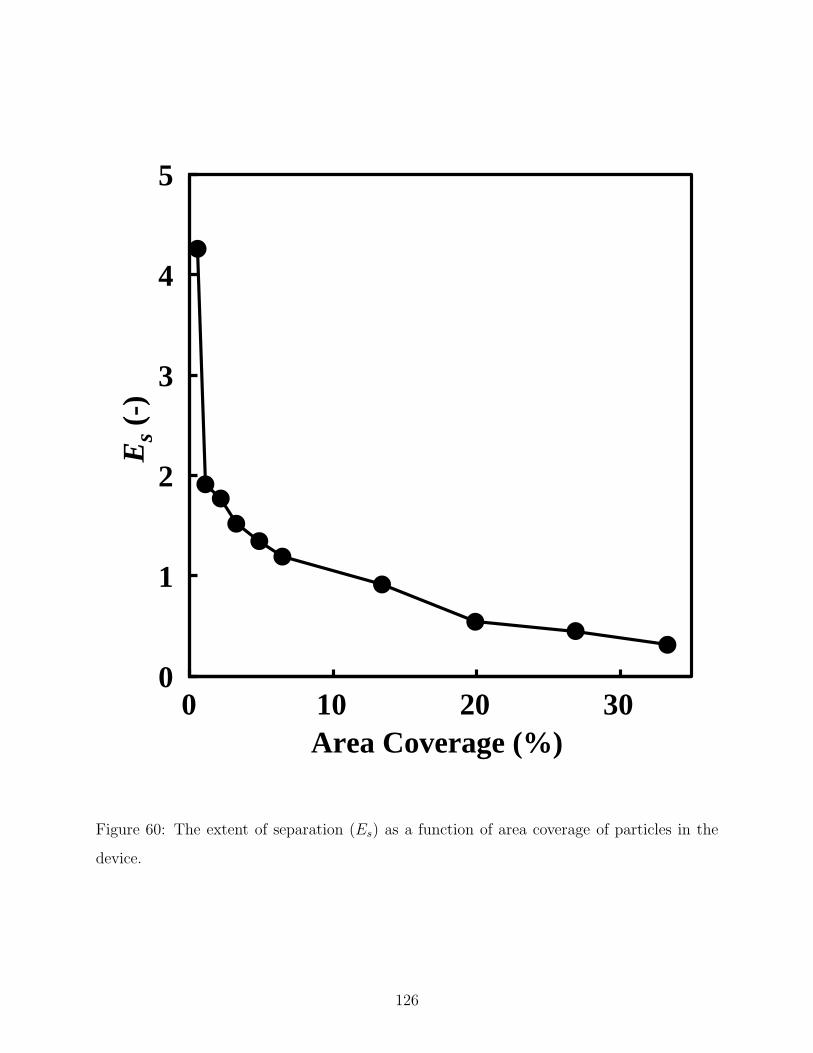
A common feature of these two rate-based separation devices is that the extent of sepa-
ration (Es) is proportional to the time (t) allowed for migration. Therefore, more migration
time can be achieved if the devices can be made to work in series (instead of a single long
device), i.e., the output of one device could be directed as the input of another, and by doing
so, the separation quality can be progressively enhanced.
150
6.4 OUTLOOK
Various solids processing industries rely on routine handling of powders and particles for
many bulk solids processes such as mixing and separation, press feeding, die filling, tableting,
packaging, bin storage, conveying, coating, etc. Solids handling is often the major bottle-neck
in the series of steps for making a final product. Practitioners are regularly asked to develop
and scale-up processes for making granular products with critical quality parameters that are
rooted in a micro-scale of scrutiny. Examples include microscale compositional variance in a
multicomponent mixture (like pet food or tablets), the microstructure of products made by
an agglomeration process, the mesoscale structural features of a particulate-filled composite,
or the effect of die filling on the structure of a pressed piece or tablet. The present work,
to some extent, aimed to elucidate the linkages between the fundamental physics of particle
flow and the industrial needs as outlined above. Though some progress has been made to
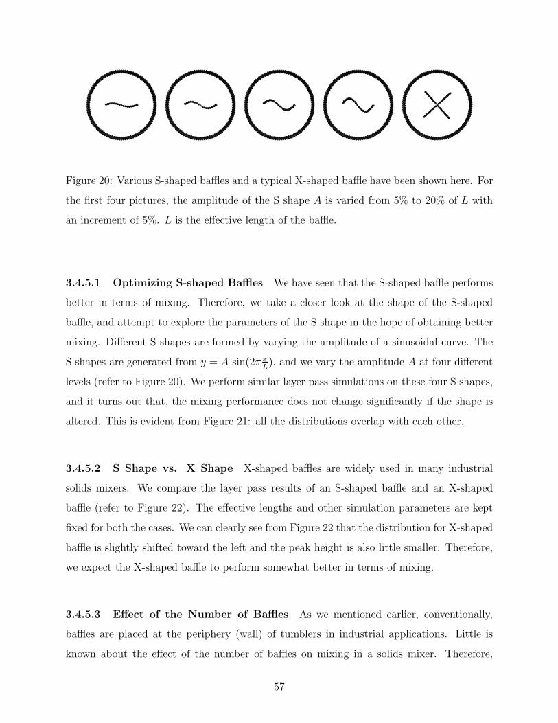
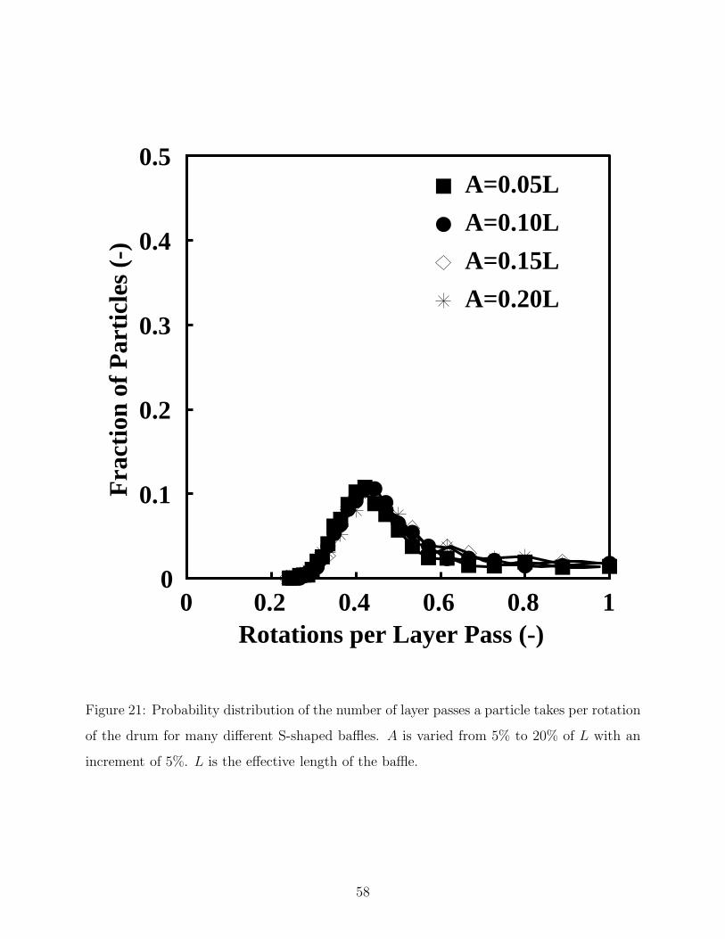
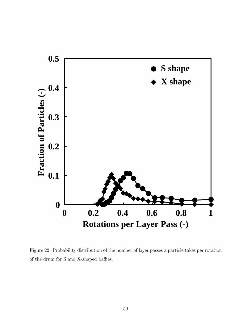
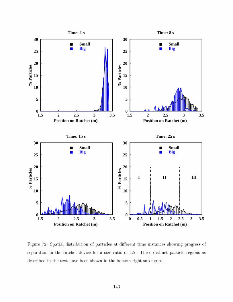
understand the segregation process [27], many formidable challenges await solutions in both
the fundamental understanding and industrially relevant applications.
Perhaps, the biggest difficulty in solids processing is the issues of scaling. The follow-
ing question would be of interest for future investigations dealing with granular flows: How
do the stress and flow fields scale when the same power ratio or specific energy input has
been utilized in a solids processing device? As a future step that is both industrially and
scientifically relevant, a combined approach including experimental investigation, simulation
and development of theory will always be helpful in searching answers to many elusive ques-
tions. The challenges in simulating large scale industrial systems are many. DEM is the gold
standard when it comes to direct numerical simulation of particle systems. At present, a
million spherical particles can be simulated using DEM on an ordinary workstation. For non-
spherical particles, however fewer can be simulated. Industrially relevant realistic systems
can easily contain 109 particles. Therefore, the direct numerical simulations at the particle
level for industrial systems is in the range of current super computers for spherical particles,
but this is not cost effective for larger systems or those containing non-spherical particles.
Therefore, a logical future research direction would be the application of high performance
computing techniques such as general purpose graphics processing units (GPGPUs) (a very
151
recent work in this direction has been performed by Radeke et al., 2010 [83]) along with the
development of faster algorithms (especially, the contact detection algorithms, which con-
sume bulk of the computing time) to speed-up calculations and make industrial scale direct
numerical simulations possible on readily available hardware (such as desktop computers or
workstations). As suggested by Williams et al. [115], the future is towards developing “smart
software” that will dynamically load the optimal algorithm for contact detection suitable for
the problem at hand.
152
APPENDIX A
OTHER STUDIES
A.1 SIMULATION OF MESOSCOPIC PHENOMENA
Throughout this dissertation, we have mostly discussed the application of particle dynamics
to simulate macroscopic phenomena. Here in this Appendix, we show how another tool
– called dissipative particle dynamics or DPD – can be used to tackle problems in the
mesoscopic length scale. We briefly review this emerging tool, its merits and demerits and
finally discuss one example where an attempt has been made to use this tool in solving a
practical problem involving droplets.
A.1.1 Non-spherical Droplet Generation
Let us turn our focus in the discussion of another exciting engineering problem involving
particles but at a different length scale: Generation of non-spherical droplets for microflu-
idic applications. Non-spherical particles, which can be processed from droplets (droplets
are used as precursors to the final particles), have a broad range of applications includ-
ing cosmetics, bio-technology, structural materials and pharmaceuticals [281]. Droplets and
particles have the potential to become important tools for drug delivery and biosensing.
Microfluidic technology holds tremendous promise [282] as it can perform typical laboratory
operations using a fraction of the volume of reagents in significantly less time. Reagents
can be tremendously reduced from milliliters and microliters to nanoliters and femtoliters
153
whereas hours of reaction time could be decreased to mere seconds or less (which is central
to the concept of “lab on a chip”). One subcategory of microfluidics is droplet-based mi-
crofluidics. Unlike continuous flow systems, droplet-based systems focus on creating discrete
volumes (nanoliters or less) with the use of immiscible phases. Droplet-based microfluidics
involves the generation and manipulation of discrete droplets. This method produces highly
monodisperse droplets in the nanometer to micrometer diameter range, at a very high rate.
Due to high surface area to volume ratios at the microscale, heat and mass transfer times
and diffusion distances are shorter, facilitating faster reaction times.
Interfacial tension between two immiscible phases naturally favors minimization of sur-
face area and this produces spherical shapes as a sphere has minimum surface area for a
given volume. Therefore, non-spherical shape is not a thermodynamically favorable state
and hence, the challenges for producing irregular shaped droplet can be easily understood.
Non-spherical shape opens up the possibility of having unique properties otherwise impos-
sible to obtain in spherical shape. For example, when converted to non-spherical particles,
they can pack more densely than spherical ones [283]. Also, irregularly shaped particles can
behave differently from spherical ones under the same hydrodynamic [284], electric, and mag-
netic conditions (see references in [281]). Since the properties of non-spherical particles are
strongly dependent on their shape, methods must be developed to control not only their size,
but also shape to obtain reproducible and uniform behavior. Though experimentally it is
possible to produce non-spherical droplets and particles using droplet-based microfluidic [282]
systems, it remains difficult to produce large quantities of monodisperse non-spherical parti-
cles of tunable geometry and adjustable properties. A literature search revealed no previous
computational work on the tuning of the shape of a droplet though experimental work on
stable non-spherical shape using interfacial particle jamming has been reported [285–287].
Therefore, in this work, we seek to address the challenges of non-spherical droplet generation
from a computational perspective. The broad objective of this part of the work is to explore
different ideas that would enable us to tune the shape of a spherical droplet by using a
computational tool called dissipative particle dynamics (DPD). The background and details
of DPD follows in the next sub-section.
154
A.1.2 Methodology: Dissipative Particle Dynamics
Dissipative particle dynamics (DPD) is an emerging technique to explore the mesoscopic
length scale (few µm). First developed by Hoogerbrugge and Koelman [288], this technique
seeks to bridge the gap between two length scales – microscopic (few nm) and mesoscopic.
DPD is a coarse graining method based on molecular dynamics (MD) [289] which can take
care of hydrodynamic behavior of complex fluids like colloids, gels, polymer melts, etc.
This method is based on the simulation of soft spheres, whose motion is governed by certain
collision rules [290], which is discussed below. In structure, a DPD algorithm looks much like
DEM or MD where particles move according to Newton’s laws. However, each DPD particle
or soft sphere represents mesoscopic description of the fluid, and does not represent individual
atoms or molecules, but loosely corresponds to “lumps” of fluids or clusters of molecules
called a “bead”. Therefore, unlike conventional molecular dynamics (MD) where we need to
know the detailed interaction between each atoms or molecules, a coarse graining is applied
in DPD and no detailed molecular level information is needed. Coarse graining results in
larger time and length scales (higher than atomistic scales) and permits the use of larger
time steps than MD simulations. Therefore, complex physical systems with hydrodynamic
behavior (complex fluids) can easily be simulated with a reasonable computational cost.
Imagine simulating a very tiny volume of a complex fluid by considering each and every
atom in the domain (as in MD, for example, one mole of something would require more than
6 × 10²³ molecules) vis-a-vis using coarse graining where each bead is a collection of many
molecules (a rough calculation using the data from Gao et al. [291] shows only 98,304 beads
will be required in DPD to simulate the same volume of fluid versus about half a million
molecules if it were simulated by classical MD).
The transport equations for a simple DPD particle i are shown in Equation A.1.
dridt
= vi ,dvi
dt=
∑
j 6=i
(FCij + FD
ij + FRij) (A.1)
where
155
FC =
aij(1− rij)rij for rij < rc
0 for rij ≥ rc(A.2)
FD = −γwD(rij)(rij · vij)rij (A.3)
FR = σwR(rij)ζij∆t−1/2rij (A.4)
In the equations above, r and v are position and velocity vectors; aij is the maximum
repulsion between particles within a pre-defined cutoff radius, rc; ζij is a random number
with zero mean and unit variance chosen independently for each pair of interacting particles
i and j, and at each time-step ∆t. The terms FC, FD and FR respectively represent:
• Conservative Force: which is a soft repulsion between particles that enforces elastic
collisions.
• Dissipative Force: which reduces the relative velocity between two particles, simulating
viscous effects.
• Random Force: which is the result of all thermal molecular motion within particles i
and j, adding heat to the system.
These forces also act along the line of centers and conserve linear and angular momentum.
The coefficients γ and σ characterize the magnitude of the dissipative and random forces,
which vanish for r > rc. Both wD and wR are weighting functions which satisfy the following
condition [292]:
wD(r) = [wR(r)]2, γ =σ2
2kBT(A.5)
Equation A.5 ensures a balance of kinetic energy within the DPD model based on the
Fluctuation-Dissipation Theorem, where kB is the Boltzmann constant and T is the tem-
perature of the system. This theorem states that a perturbation within a system at the
molecular level dissipates as the system returns to equilibrium [293–295]. In essence, FD
and FR serve as a thermostat in order to maintain the temperature, ensuring the system is
not artificially heated.
156
A.1.3 Boundary Conditions
The manner in which the walls are prescribed in DPD is an unresolved matter in the lit-
erature. Wall particles are “frozen” (i.e., of the lowest thermal energy within the system),
but the soft repulsion between particles does not prevent actual fluid elements from “pen-
etrating” the wall. In addition, there is the problem of the wall particles decreasing the
overall fluid temperature. Various researchers have sought to combat this by analytically
solving for effective wall forces [296], increasing the density of particles at the wall [297], or
by introducing a random velocity distribution (with fixed mean) for the wall particle [295].
DPD time and length scale calculation has been described by Moeendarbary et al. [298].
These units allow us to model systems with length scales from nanometers to micrometers
and overall time scales of up to a few seconds.
A.1.4 Results: Non-spherical Droplet Generation
Since a spherical shape is the most stable configuration for a droplet, we employ a few charged
particles (“stabilizers”) to perturb the stable spherical state. Equation A.6 shows the
repulsive force between a charged particle pair, which in essence, is a Coulombic interaction:
FQ =1
4πε0
qiqjr2
rij (A.6)
where ε0 is the dielectric constant of the medium, qi and qj are charges on the particles
and r is the separation distance between particles. If both charges have the same sign (like
charges) then the product qiqj is positive and the direction of the force on qi is given by
rji; the charges repel each other. If the charges have opposite signs then the product qiqj
is negative and the direction of the force on qi is given by −rji; the charges attract each
other. In a typical simulation, we use three kinds of DPD particles/beads: droplet, solvent
and stabilizer particles. The initial configuration is a cluster of droplet particles in a near
spherical shape in the matrix of solvent particles. The droplet particles are surrounded by
charged stabilizer particles. A typical initial configuration is shown in Figure 75 along with
an intermediate stage, which shows that DPD can be used to tune the shape of a spherical
droplet.
157
Figure 75: (Left) Initial spherical shape of a DPD droplet consisting of 22,528 particles
(red). Eight (8) charged particles (blue) are positioned at the corners of a cube enclosing the
spherical droplet. There are 90,112 solvent particles which are not shown here for clarity.
(Right) Intermediate stage showing the evolution of the non-spherical shape.
A.1.5 Outlook
In future, the following further studies are proposed to systematically investigate the real-
ization of a non-spherical droplet:
1. Assessing different initial configurations: In order to get a droplet in cubic, tetra-
hedral or bipyramidal shape, one needs to change the orientation and numbers of the
stabilizer particles. Therefore, examination of the effects of different initial configurations
on the final shape of the droplet is a good starting point.
2. Exploring the parameters space: The parameter aij determines the magnitude of
the maximum repulsive force between a pair of DPD particles, i and j. Exploration of
the parameters space by changing aij and the charges qi on the stabilizer particles would
158
aid in identifying proper parameters for a desired shape.
3. Evaluating size effects: Since the system sizes accessible to simulations are rather
small, one can draw conclusions about the behavior of larger real systems by investigating
the size effects, i.e., how the system properties will vary with the system size. This can
be evaluated by using different volumes of the simulation box.
4. Evaluating density effects: The system density ρ (equal to the number of DPD parti-
cles per unit volume) determines how many total particles will be in the simulation box.
Typically, the density chosen is a free parameter, but since the number of interactions
for each particle increases linearly with the density, the required computation time (CPU
time) t per time-step and per unit volume increases as ρ2 [290]. Therefore, for efficiency
reason, many workers used a value of ρ = 3.0, which is the lowest possible density where
the scaling relation for excess pressure in the equation of state still holds good. However,
the effect of density on final droplet shape is not clear and this can be a topic of future
investigations.
5. Exploring other ideas: Using armored particle layers around a droplet to stabilize a
non-spherical shape by jamming the interface is a fairly common practice [281,285–287,
299,300]. Such techniques can be implemented in the droplet simulation to stabilize the
non-spherical shape.
159
APPENDIX B
NOMENCLATURE
English Symbols
2S center-to-center peg spacing (Ch. 5)
A a factor equal to ±1 (Ch. 5)
Av amplitude of vibration of ratchet device (Ch. 5)
a radius of contact spot (Ch. 2)
(a) asymmetry parameter of ratchet tooth (Ch. 5)
aij maximum repulsion between particles i and j (Appendix A)
C concentration of tracer particle (Ch. 2)
〈C〉 mean concentration of tracer particle (Ch. 2)
c dimensionless collisional viscosity (Ch. 3)
(c) concentration (Ch. 4)
D drum diameter (Ch. 3)
(D) (particle) diffusivity (Ch. 4)
d particle diameter (Ch. 3)
(d) diameter of largest particle in a ratchet device (Ch. 5)
d particle size ratio (Ch. 3, 4)
deff effective diameter of a particle (Ch. 5)
dp diameter of a particle (Ch. 5)
dt time-step (Ch. 2)
E elastic modulus (Ch. 2)
E∗ effective elastic modulus (Ch. 2)
Ei elastic modulus of particle i (Ch. 2)
Es extent of separation (Ch. 5)
160
English Symbols
eijn normal unit vector (Ch. 2)
eijt tangential unit vector (Ch. 2)
FCij conservative force on particle i due to particle j in DPD (Ap-
pendix A)
FDij dissipative force on particle i due to particle j in DPD (Appendix
A)
f number fraction of segregating species (Ch. 3)
(f) frequency of vibration of ratchet device (Ch. 5)
fcrit critical forcing frequency (Ch. 3, 4)
fe effective forcing frequency (Ch. 3)−→Fij force on particle i due to particle j (vector) (Ch. 2)−−→Fij
n normal force on particle i due to particle j (vector) (Ch. 2)−→F tij tangential force on particle i due to particle j (vector) (Ch. 2)
−→Fn normal force (vector) (Ch. 2)−→Ft tangential force (Ch. 2)
F nij normal force on particle i due to particle j (Ch. 2)
F tij tangential force on particle i due to particle j (Ch. 2)
Fmax maximum force (Ch. 2)
Fn normal force (Ch. 2)
FQ Coulombic force (Appendix A)
FRij random force on particle i due to particle j in DPD (Appendix
A)
Fr Froude number (Ch. 3)
Ft tangential force at particle-particle contact (Ch. 2)
Fto old tangential force (Ch. 2)
Fy yield force (Ch. 2)
G shear modulus (Ch. 2)
G∗ effective shear modulus (Ch. 2)
Gi shear modulus of particle i (Ch. 2)−→g acceleration due to gravity (vector) (Ch. 2)
g acceleration due to gravity (Ch. 3)
H particle bed height in a chute (Ch. 4)
(H) height of simulation box (Ch. 5)
Hp vertical center-to-center peg spacing (Ch. 5)
h ratchet tooth height (Ch. 5)
h(x, t) height of a dynamic sand pile (Ch. 2)
Ip moment of inertia of a particle (Ch. 2)
JS segregation flux (Ch. 4)
161
English Symbols
KS segregation constant, size (Ch. 3, 4)
KT segregation constant, density (Ch. 3, 4)
kB Boltzmann constant (Appendix A)
kn normal force constant (Ch. 2)
kt tangential stiffness (Ch. 2)
ky plastic stiffness (Ch. 2)
L effective baffle length (Ch. 3)
(L) chute length (Ch. 4)
(L) separation device length or length of simulation box (Ch. 5)
Lplug length of particle plug on chute (Ch. 4)
l length of the projection of the longer side of ratchet tooth on
horizontal (Ch. 5)
ML Lacey mixing index (Ch. 2)
MP Poole mixing index (Ch. 2)
mp mass of a particle (Ch. 2)
N total number of particles (Ch. 2, 3, 4)
Nc number of concentration measurement locations (Ch. 2, 3)
Nh number of particle layers (Ch. 5)
Pe segregation-based Peclet number (Ch. 4)
p depth of a ratchet tooth (Ch. 5)
qi charge on particle i (Appendix A)
R ratio of contact curvature due to plastic deformation and effec-
tive radius (Ch. 2)−→R radius of particle (vector) (Ch. 2)
R radius of a particle (Ch. 2)
(R) drum radius (Ch. 3)
(R) degree of mixing (Ch. 4)
R∗ effective radius (Ch. 2)
R1 radius of small particle (Ch. 4)
Rp contact curvature due to plastic deformation (Ch. 2)
(Rp) radius of a particle (Ch. 5)
Rpeg radius of a peg (Ch. 5)
R(x, t) thickness of rolling layer (Ch. 2)−→ri radius of particle i (vector) (Ch. 2)
r radius of a particle (Ch. 2)
(r) separation distance between particles (Appendix A)
ri position vector of a DPD particle (Appendix A)
rij vector connecting centers of two DPD particles i and j (Ap-
pendix A)
162
English Symbols−→rj radius of particle j (vector) (Ch. 2)
Sij separation between centers of particle i and particle j (Ch. 2)
T total contact detection time (Ch. 2)
(T ) granular temperature (Ch. 4)
(T ) temperature of a DPD system (Appendix A)
t dimensionless time (Ch. 4)
t time allowed for migration of particles (Ch. 5)
tc duration of collision (Ch. 2)
tD diffusion time (Ch. 4)
tentry particle entry time on chute (Ch. 4)
texit particle exit time from chute (Ch. 4)
tS characteristic segregation time (Ch. 3, 4)
Uavg average stream-wise flow velocity of particles in a chute (Ch. 4)
u velocity of particle (Ch. 4)
〈Vbig〉 average longitudinal velocity of big particles (Ch. 5)
〈Vsmall〉 average longitudinal velocity of small particles (Ch. 5)−→vi velocity of particle i (vector) (Ch. 2)−→vj velocity of particle j (vector) (Ch. 2)−→vp particle velocity (vector) (Ch. 2)
vi velocity vector of a DPD particle (Appendix A)
vS segregation velocity (Ch. 3)
vt tangential velocity (Ch. 2)
W width or depth of simulation box (Ch. 5)
Wi full width at half max (FWHM) for distribution of particle type
i (Ch. 4)
w ratchet tooth width (Ch. 5)
wD weighting function for dissipative force in DPD (Appendix A)
wR weighting function for random force in DPD (Appendix A)
Xc scaled difference of particle mass centers on chute (Ch. 4)
Xc centroid of particle mass on chute (Ch. 4)
xt velocity at time t (Ch. 2)
xt position at time t (Ch. 2)
zp z coordinate of a particle (Ch. 5)
zpeg z coordinate of the center of a peg (Ch. 5)
163
Greek Symbols
α computational overlap between contacting particles (Ch. 2)
(α) a fitting parameter (Ch. 4)
α relative normal velocity of particles in contact (Ch. 2)
αmax maximum deformation (Ch. 2)
αo a constant in time-step equation (Ch. 2)
αy deformation at yield point (Ch. 2)
β a fitting parameter (Ch. 4)
βm dynamic angle of repose of granular materials (Ch. 3)
βs angle of repose of granular materials (Ch. 3)
Γ dimensionless acceleration of ratchet device (Ch. 5)
γ magnitude of dissipative force in DPD (Appendix A)
γ shear rate (Ch. 4)
γn damping parameter (Ch. 2)
γo shear rate at midpoint of layer in a tumbler (Ch. 3)
∆s tangential displacement (Ch. 2)
∆t time-step (Ch. 2)
δo maximum shear layer thickness (Ch. 3)
ε0 dielectric constant (Appendix A)
ζij a random number with zero mean and unit variance (Appendix
A)
λ wave speed (Ch. 2)
ν Poisson ratio (Ch. 2)
(ν) solid volume fraction (Ch. 4)
νi Poisson ratio for particle i (Ch. 2)
ξ a fitting parameter (Ch. 3)
ρ density (Ch. 2)
σ standard deviation of the composition of a mixture (Ch. 2)
σMIX standard deviation of the composition of a completely mixed
mixture (Ch. 2)
σSEG standard deviation of the composition of a completely segregated
mixture (Ch. 2)
σy yield stress (Ch. 2)
τmean mean residence time of particle in layer (Ch. 3)
φi concentration of species i (Ch. 4)
φt total solids volume fraction (Ch. 4)
ω drum rotation rate (Ch. 3)−→ωp angular velocity of a particle (vector) (Ch. 2)
164
Abbreviations
AVCHD advanced video codec high definition (Ch. 5)
BCRE Bouchaud, Cates, Ravi & Edwards (model) (Ch. 2)
BdG Boutreux & de Gennes (model) (Ch. 2)
CAD computer aided design (Ch. 2)
CCD charge-coupled device (Ch. 5)
CDF cumulative distribution function (Ch. 4)
CPU central processing unit (Ch. 2)
DEM discrete element method (Ch. 1-6)
DNA deoxyribonucleic acid (Ch. 5)
DPD dissipative particle dynamics (Appendix A)
DV digital video (Ch. 5)
FWHM full width at half max (Ch. 4)
GNU GNU’s not Unix (Ch. 4)
GPGPU (GPU) general purpose graphics processing units (Ch. 2, 6)
HPC high performance computing (Ch. 2, 6)
HSI hue-saturation-intensity (Ch. 5)
IS intensity of segregation (Ch. 2, 3, 4)
MC Monte Carlo (simulation) (Ch. 4)
MD molecular dynamics (Ch. 2, Appendix A)
NBS no binary search (Ch. 2)
OOP object-oriented programming (Ch. 2)
PD particle dynamics (Ch. 1)
PMMA polymethylmethacrylate (Ch. 4)
RGB red-green-blue (Ch. 5)
RPM revolutions per minute (Ch. 3)
RSD relative standard deviation (Ch. 2, 4)
165
Subscripts
1 small or segregating species
avg average
B Boltzmann
big big
c collision or centroid or cell
crit critical
D diffusion
e effective
eff effective
entry entry
exit exit
i particle i
ij on particle i due to particle j
j particle j
L Lacey
max maximum
n normal
o old
P Poole
p particle
peg peg
plug plug
S segregation or size
s separation
small small
T density
t tangential or at time t
y yield
Superscripts
C conservative
D,D dissipative
n normal
Q Coulombic
R,R random
t tangential
166
BIBLIOGRAPHY
[1] Isabel Margarita Figueroa Amenabar. Exploring analogies between granular materialsand fluids. PhD thesis, University of Pittsburgh, 2009.
[2] P. A. Cundall and O. D. L. Strack. A discrete numerical model for granular assemblies.Geotechnique, 29:47–65, 1979.
[3] A. Munjiza and K. R. F. Andrews. NBS contact detection algorithm for bodies ofsimilar size. International Journal for Numerical Methods in Engineering, 43(1):131–149, 1998.
[4] Watson L. Vargas-Escobar. Discrete Modeling of Heat Conduction in Granular Media.PhD thesis, University of Pittsburgh, Pittsburgh, 2002.
[5] http://www.mgm.ms.unimelb.edu.au/about.php, last accessed 4th September, 2011.
[6] B. J. Ennis, J. Green, and R. Davies. The legacy of neglect in the US. ChemicalEngineering Progress, 90(4):32–43, 1997.
[7] R. M. Nedderman. Statics and Kinematics of Granular Materials. Cambridge Univer-sity Press, 1992.
[8] F. J. Muzzio, C. L. Goodridge, A. Alexander, P. Arratia, H. Yang, O. Sudah, andG. Mergen. Sampling and characterization of pharmaceutical powders and granularblends. International Journal of Pharmaceutics, 250:51–64, 2003.
[9] P. P. Thomas and Y. B. G. Varma. Fluidised bed frying of granular food materials.Powder Technology, 69:213–222, 1992.
[10] Amit Chatterjee, A. Sathe, M. Srivastava, and P. Mukhopadhyay. Flow of materialsin rotary kilns used for sponge iron manufacture: Part I. Effect of some operationalvariables. Metallurgical and Materials Transactions B, 14(3):375–381, 1983.
[11] Dennis R. Van Puyvelde. Simulating the mixing and segregation of solids in the trans-verse section of a rotating kiln. Powder Technology, 164:1–12, 2005.
167
[12] S Pirard, G Lumay, N Vandewalle, and J Pirard. Motion of carbon nanotubes in arotating drum: The dynamic angle of repose and a bed behavior diagram. ChemicalEngineering Journal, 146(1):143–147, 2009.
[13] R. L. Brown. The fundamental principles of segregation. Inst. Fuel, 13:15–19, October1939.
[14] J. C. Williams. The segregation of particulate materials. Powder Technol., 15:245–251,1976.
[15] T. Mullin. Mixing and de-mixing. Science, 295:1851, 2002.
[16] J.M. Ottino and D.V. Khakhar. Mixing and segregation of granular materials. Ann.Rev. Fluid Mech., 32:55–91, 2000.
[17] S.L. Conway, T. Shinbrot, and B.J. Glasser. A taylor vortex analogy in granular flows.Nature, 431:433–437, 2004.
[18] K. M. Hill, D. V. Khakhar, J. F. Gilchrist, J. J. McCarthy, and J. M. Ottino.Segregation-driven organization in chaotic granular flows. PNAS, 96:11701–11706,1999.
[19] Hernan A. Makse, S. Havlin, P. R. King, and H. E. Stanley. Spontaneous stratificationin granular mixtures. Nature, 386:379–381, 1997.
[20] O. Pouliquen, J. Delour, and S. B. Savage. Fingering in granular flows. Nature,386:816–817, 1997.
[21] D. V. Khakhar, J. J. McCarthy, and J. M. Ottino. Radial segregation of granularmixtures in rotating cylinders. Phys. Fluids, 9:3600–3614, 1997.
[22] J. B. Knight, H. M. Jaeger, and S. R. Nagel. Vibration-induced size separation ingranular media: The convection connection. Phys. Rev. Lett., 70:3728–3730, 1993.
[23] N. Burtally, P. J. King, and M. R. Swift. Spontaneous air-driven separation in verticallyvibrated fine granular mixtures. Science, 295:1877–1879, 2002.
[24] J. M. Ottino. The kinematics of mixing: stretching, chaos, and transport. CambridgeUniveristy Press, New York, 1989.
[25] P. Tang and V. M. Puri. Methods for minimizing segregation: A review. ParticulateScience and Technology, 22:321–337, 2004.
[26] H. M. Jaeger, S. R. Nagel, and R. P. Behringer. Granular solids, liquids and gases.Rev. Mod. Phys., 68:1259–1273, 1996.
168
[27] J. M. Ottino and D. V. Khakhar. Fundamental research in heaping, mixing, andsegregation of granular materials: challenges and perspectives. Powder Technology,121:117–122, 2001.
[28] J. Bridgwater. Fundamental powder mixing mechanisms. Powder Technology, 15:215–231, 1976.
[29] M. B. Donald and B. Roseman. Mixing and de-mixing of solid particles: Part I.mechanisms in a horizontal drum mixer. Brit. Chem. Eng., 7:749 – 752, 1962.
[30] D. V. Khakhar, J. J. McCarthy, and J. M. Ottino. Mixing and segregation of granularmaterials in chute flows. Chaos, 9:594–610, 1999.
[31] Deliang Shi, Adetola A. Abatan, Watson L. Vargas, and J. J. McCarthy. Eliminatingsegregation in free-surface flows of particles. Physical Review Letters, 99:148001, 2007.
[32] M. Kwapinska, G. Saage, and E. Tsotsas. Continous versus discrete modelling of heattransfer to agitated beds. Powder Technology, 181:331–342, 2008.
[33] B. Chaudhuri, F. J. Muzzio, and M. S. Tomassone. Modeling of heat transfer ingranular flow in rotating vessels. Chemical Engineering Science, 61:6348–6360, 2006.
[34] W. L. Vargas and J. J. McCarthy. Heat conduction in granular materials. AIChEJournal, 47:1052–1059, 2001.
[35] D. K. Kafui and C. Thornton. Fully-3D DEM simulation of fluidised bed spray granu-lation using an exploratory surface energy-based spray zone concept. Powder Technol.,184(2):177 – 188, May 2008.
[36] Julio M. Ottino. The art of mixing with an admixture of art: Fluids, solids, and visualimagination. Physics of Fluids, 22(2):021301+, 2010.
[37] Heinrich Jaeger, Sidney Nagel, and Robert Behringer. The physics of granular mate-rials. Physics Today, 49(4):32–38, 1996.
[38] P. G. de Gennes. Granular matter: a tentative view. Rev. Mod. Phys., 71:S374–S382,1999.
[39] S. B. Savage and C. K. K. Lun. Particle size segregation in inclined chute flow ofcohesionless granular solids. J. Fluid Mech., 189:311–335, 1988.
[40] N. Standish. Principles in burdening and bell-less charging. Nimaroo Publishers,,Wollongong, Australia, 1st edition, 1979.
[41] J. Li, A. B. Yu, J. Bridgwater, and S. L. Rough. Spontaneous inter-particle percolation:A kinematic simulation study. Powder Technology, 203(2):397 – 403, January 2010.
169
[42] S. R. De Silva, A. Dyroy, and G. G. Enstad. Segregation mechanism and their quan-tification using segregation testers. In A. D. Rosato and D. L. Blackmore, editors,Segregation in Granular Flows, IUTAM Symposium Series, pages 11–29. Kluwer Aca-demic Press, 2000.
[43] J. C. Williams. The segregation of powders and granular materials. Fuel Soc. J.,14:29–35, 1963.
[44] J. C. Williams and M. I. Khan. The mixing and segregation of particulate solids ofdifferent particle size. Chem. Eng., 269:19–25, 1973.
[45] H. Matthee. Segregation phenomena relating to bunkering of bulk materials: Theoret-ical considerations and experimental investigations. Powder Technology, 1(5):265–271,February 1968.
[46] Tatsuo Tanaka. Segregation models of solid mixtures composed of different densitiesand particle sizes. Industrial & Engineering Chemistry Process Design and Develop-ment, 10(3):332–340, 1971.
[47] J. Masliyah and J. Bridgwater. Particle percolation: A numerical study. Trans. Inst.Chem. Engrs., 52:31–52, 1974.
[48] J. Bridgwater, M. H. Cooke, and A. M. Scott. Interparticle percolation: equipmentdevelopment and mean percolation velocities. Trans. Inst. Chem. Eng., 56:157, 1978.
[49] J. A. Drahun and J. Bridgwater. The mechanisms of free surface segregation. PowderTechnology, 36(1):39 – 53, 1983.
[50] Hernan Makse, Shlomo Havlin, Peter King, and Eugene Stanley. Spontaneous strati-fication in granular mixtures. Nature, 386(6623):379–382, 1997.
[51] Y. Kajiwara, T. Inada, and T. Tanaka. Two dimensional analysis on the formationprocess of burden distribution at blast furnace top. Trans. ISIJ, 28:916, 1988.
[52] T. Tanaka, Y. Kajiwara, T. Inada, and C. Yamagata. Flow dynamics of granularmaterials in a blast furnace. In Ironmaking Conference Proceedings, page 237, 1988.
[53] T. Inada, Y. Kajiwara, and T. Tanaka. A mathematical model for particle size dis-tribution in bell-type charging at blast furnace top. ISIJ International, 29(9):761,1989.
[54] J. P. Bouchaud, M. E. Cates, J. R. Prakash, and S. F. Edwards. A model for thedynamics of sandpile surfaces. J. Phys. I, France, 4:1383, 1994.
[55] A. Mehta, editor. Granular matter: an interdisciplinary approach. Springer-Verlag,New York, 1994.
170
[56] P.-G. de Gennes. Surface dynamics of a granular material. C. R. Acad. Sci. (Paris),321(II):501, 1995.
[57] T. Boutreux and P. G. de Gennes. Surface flows of granular mixtures. I. Generalprinciples and minimal model. J. Phys. I, France, 6:1295–304, 1996.
[58] T. Boutreux. PhD Thesis. PhD thesis, Paris VI University, Paris, 1998.
[59] T. Boutreux. Surface flows of granular mixtures: II. Segregation with grains of differentsize. The European Physical Journal B - Condensed Matter and Complex Systems,6(3):419–424, 1998.
[61] T. Boutreux, H. A. Makse, and P. G. de Gennes. Surface flows of granular mixtures.The European Physical Journal B - Condensed Matter and Complex Systems, 9(1):105–115, 1999.
[62] Pierre Jop, Yoal Forterre, and Olivier Pouliquen. A constitutive law for dense granularflows. Nature, 441(7094):727–730, 2006.
[63] C. Campbell. Granular material flows – an overview. Powder Technology, 162(3):208–229, 2006.
[64] H. Zhu, Z. Zhou, R. Yang, and A. B. Yu. Discrete particle simulation of particulatesystems: A review of major applications and findings. Chemical Engineering Science,63(23):5728–5770, 2008.
[65] C. Thornton (Guest Editor). Special issue on numerical simulations of discrete particlesystems. Powder Technology, 109:3–292, 2000.
[66] J. P. Bardet. Introduction to computational granular mechanics. In B. Cambou, editor,Behavior of granular materials, pages 99–169. Springer-Verlag, 1998.
[67] K. Z. Y. Yen and T. K. Chaki. A dynamic simulation of particle rearrangement inpowder packings with realistic interactions. Journal of Applied Physics, 71:3164–3173,1992.
[68] C. Thornton and C. W. Randall. Applications of theoretical contact mechanics to solidparticle system simulation. In M. Satake and J. T. Jenkins, editors, Micromechanicsof Granular Material, pages 133–142. Elsevier Science Publishers, Amsterdam, 1988.
[69] M. Satake. Constitution of mechanics of granular materials through the graph theory.In S. C. Cowin and M. Satake, editors, U.S.-Japan Seminar in Continuum Mechanicsand Statistical Approaches in the Mechanics of Granular Materials, pages 47–62, 1978.
171
[70] Q. M. Tai and M. H. Sadd. A discrete element study of the relationship of fabricto wave propagational behaviours in granular material. Int. J. Numer. Anal. Meth.Geomech., 21:295–311, 1997.
[71] Y. Kaneko, T. Shiojima, and M. Horio. DEM simulation of fluidized beds for gas-phaseolefin polymerization. Chemical Engineering Science, 54:5809–5821, 1999.
[72] Y. Tsuji, T. Kawaguchi, and T. Tanaka. Discrete particle simulation of two-dimensionalfluidized bed. Powder Technology, 77:79–87, 1993.
[73] O. R. Walton and R. L. Braun. Viscosity, granular-temperature, and stress calculationsfor shearing assemblies of inelastic, frictional disks. J. Rheol., 30:949–980, 1986.
[74] H. J. Herrmann and S. Luding. Modeling granular media on the computer. ContinuumMech. Thermodyn., 10:189–231, 1998.
[75] C. S. Campbell. Rapid granular flows. Ann. Rev. Fluid Mech., 22:57–90, 1990.
[76] Ng T-T. Small-strain response of random arrays of spheres using DEM. J. Eng. Mech.,122:239–244, 1996.
[77] C. Thornton. Force transmission in granular media. KONA, 15:81–90, 1997.
[78] R. Yang, R. Zou, K. Dong, X. An, and A. Yu. Simulation of the packing of cohesiveparticles. Computer Physics Communications, 177(1-2):206–209, July 2007.
[79] C. Thornton, K. K. Yin, and M. J. Adams. Numerical simulation of the impact fractureand fragmentation of agglomerates. Journal of Physics D: Applied Physics, 29:424–435,1996.
[80] J. J. McCarthy. Micro-modeling of cohesive mixing processes. Powder Technol., 138(1):63–67, 2003.
[81] M. P. Allen and D. J. Tildesley. Computer Simulation of Liquids. Clarendon Press,Oxford, 1987.
[82] H. Zhu, Z. Zhou, R. Yang, and A. B. Yu. Discrete particle simulation of particulatesystems: Theoretical developments. Chemical Engineering Science, 62(13):3378–3396,2007.
[83] Charles Radeke, Benjamin Glasser, and Johannes Khinast. Large-scale powder mixersimulations using massively parallel GPU architectures. Chemical Engineering Science,65(24):6435–6442, 2010.
[84] J. Roth, F. Gahler, and H.-R. Trebin. A molecular dynamics run with 5 180 116 000particles. International Journal of Modern Physics C, 11(2):317–322, 2000.
172
[85] Kai Kadau, Timothy Germann, and Peter Lomdahl. Molecular dynamics comes of age:320 billion atom simulation on BlueGene/L. International Journal of Modern PhysicsC, 17(12):1755–1761, 2006.
[86] Thorsten Poschel and Thomas Schwager. Computational Granular Dynamics (Modelsand Algorithms). Springer, Berlin, Heidelberg, New York, 2005.
[87] C. S. Campbell and C. E. Brennen. Chute flows of granular material: some computersimulations. Journal of Applied Mechanics, 52:172–178, 1985.
[88] K. L. Johnson. Contact Mechanics. Cambridge University Press, Cambridge, 1987.
[89] H. Hertz. ueber die beruhrung fester elastischer korper. J. f. reine u. angewandteMath., 92:1–15, 1882.
[90] J. Lee and H. J. Herrmann. Angle of repose and angle of marginal stability: moleculardynamics of granular particles. Journal of Physics A, 26:373–383, 1993.
[91] J. T. Oden and J. A. C. Martins. Models and computational methods for dynamicfriction phenomena. Computer Methods in Applied Mechanics and Engineering, 52(1-3):527–634, 1985.
[92] V. Buchholtz and T. Poschel. Numerical investigations of the evolution of sandpiles.Physica A, 202:390–401, 1994.
[93] R. D. Mindlin and H. Deresiewicz. Compliance of elastic bodies in contact. J. Appl.Mech., 20:327, 1953.
[94] J. Schafer, S. Dippel, and E. Wolf. Force schemes in simulations of granular materials.J. Phys. I, 67:1751–1776, 1991.
[95] J. J. McCarthy and J. M. Ottino. Particle dynamics simulation: A hybrid techniqueapplied to granular mixing. Powder Technology, 97:91–99, 1998.
[96] A. Di Renzo. Comparison of contact-force models for the simulation of collisions inDEM-based granular flow codes. Chemical Engineering Science, 59(3):525–541, Febru-ary 2004.
[97] H. Kruggel-Emden, E. Simsek, S. Rickelt, S. Wirtz, and V. Scherer. Review andextension of normal force models for the discrete element method. Powder Technology,171(3):157–173, February 2007.
[98] S. T. Nase, W. L. Vargas, A. A. Abatan, and J. J. McCarthy. Discrete characterizationtools for wet granular media. Powder Technol., 116:214–223, 2001.
[99] C. Thornton and Z. Ning. A theoretical model for the stick/bounce behavior of adhe-sive, elastic-plastic spheres. Powder Technology, 99:154–162, 1998.
173
[100] J. J. McCarthy, V. Jasti, M. Marinack, and C. F. Higgs. Quantitative validation of thediscrete element method using an annular shear cell. Powder Technology, 203(1):70 –77, October 2010.
[101] Y. C. Zhou, B. H. Xu, A. B. Yu, and P. Zulli. Numerical investigation of the angle ofrepose of monosized spheres. Physical Review E, 64(2), 07 2001.
[102] J. A. Greenwood, H. Minshall, and D. Tabor. Hysteresis losses in rolling and slidingfriction. Proceedings of the Royal Society of London. Series A, Mathematical andPhysical Sciences, 259(1299):480–507, 1961.
[103] N. V. Brilliantov and T. Poschel. Rolling as a “continuing collision”. The EuropeanPhysical Journal B - Condensed Matter and Complex Systems, 12(2):299–301, 1999.
[104] N. V. Brilliantov and T. Poschel. Rolling friction of a viscous sphere on a hard plane.EPL (Europhysics Letters), 42(5):511+, June 1998.
[105] L. Verlet. Computer experiments on classical fluids. I. Thermodynamical properties ofLennard-Jones molecules. Physical Review, 159(1):98 – 103, 1967.
[106] G. Grest. Vectorized link cell Fortran code for molecular dynamics simulations for alarge number of particles. Computer Physics Communications, 55(3):269–285, 1989.
[107] B. Mirtich. Impulse-based dynamic simulation of rigid body systems. PhD thesis,University of California, Berkeley, California, 1988.
[108] Javier Bonet and Jaime Peraire. An alternating digital tree (ADT) algorithm for 3Dgeometric searching and intersection problems. International Journal for NumericalMethods in Engineering, 31(1):1–17, 1991.
[109] R. OConnor, J. Gill, and J. R. Williams. A linear complexity contact detection algo-rithm for multi-body simulation. In Proc. 2nd U.S. Conf. on Discrete Element Methods,pages 53 – 64, MIT, MA, 1993.
[110] Mats Oldenburg and Larsgunnar Nilsson. The position code algorithm for contactsearching. International Journal for Numerical Methods in Engineering, 37(3):359–386, 1994.
[111] Eric Perkins and John R. Williams. A fast contact detection algorithm insensitiveto object sizes. Engineering Computations: Int J for Computer-Aided Engineering,18(1/2):48–62, 2001.
[112] Jean-Albert Ferrez. Dynamic triangulations for efficient 3D simulation of granularmaterials. PhD thesis, EPFL, Lausanne, EPFL, 2001.
[113] Z. Yao. Improved neighbor list algorithm in molecular simulations using cell decompo-sition and data sorting method. Computer Physics Communications, 161(1-2):27–35,2004.
174
[114] E. Nezami, Y. Hashash, D. Zhao, and J. Ghaboussi. A fast contact detection algorithmfor 3-D discrete element method. Computers and Geotechnics, 31(7):575–587, 2004.
[115] John Williams, Eric Perkins, and Ben Cook. A contact algorithm for partitioning N ar-bitrary sized objects. Engineering Computations: International Journal for Computer-Aided Engineering and Software, 21(2 – 4):235–248, 2004.
[116] D. Mason. Faster neighbour list generation using a novel lattice vector representation.Computer Physics Communications, 170(1):31–41, 2005.
[117] A. Munjiza, E. Rougier, and N. W. M. John. MR linear contact detection algorithm.International Journal for Numerical Methods in Engineering, 66(1):46–71, 2006.
[118] K. Han, Y. T. Feng, and D. R. J. Owen. Performance comparisons of tree-basedand cell-based contact detection algorithms. Engineering Computations: InternationalJournal for Computer-Aided Engineering and Software, 24(2):165–181, 2007.
[119] Rainald Lohner. The empty bin: A data structure for spatial search of time-varyingdata. Communications in Numerical Methods in Engineering, 23(12):1111–1119, 2007.
[120] Kejing He, Shoubin Dong, and Zhaoyao Zhou. Multigrid contact detection method.Physical Review E, 75(3):036710, 2007.
[121] Hiroshi Mio, Atsuko Shimosaka, Yoshiyuki Shirakawa, and Jusuke Hidaka. Cell opti-mization for fast contact detection in the discrete element method algorithm. AdvancedPowder Technology, 18(4):441–453, 2007.
[122] John Peters, Raju Kala, and Robert Maier. A hierarchical search algorithm for dis-crete element method of greatly differing particle sizes. Engineering Computations:International Journal for Computer-Aided Engineering and Software, 26(6):621–634,2009.
[123] Luyi Lu, Zhaolin Gu, Kangbin Lei, Sheng Wang, and Kiwamu Kase. An efficientalgorithm for detecting particle contact in non-uniform size particulate system. Par-ticuology, 8(2):127–132, 2010.
[124] Wan-Qing Li, Tang Ying, Wan Jian, and Dong-Jin Yu. Comparison research on theneighbor list algorithms: Verlet table and linked-cell. Computer Physics Communica-tions, 2010.
[125] M. Moore and J. Wilhelms. Collision detection and response for computer animation.Computer Graphics, 22(4):289–298, 1988.
[126] M. C. Lin. Efficient collision detection for animation and robotics. PhD thesis, Uni-versity of California, Berkeley, California, 1993.
[127] J. C. Latombe. Robot motion planning. Kluwer Academic Press, 1991.
175
[128] F. P. Preparata and M. I. Shamos. Computational geometry. Springer-Verlag, NewYork, 1985.
[129] H. Samet. Spatial data structures: quadtree, octrees and other hierarchical methods.Addison Wesley, 1989.
[130] Tathagata Bhattacharya and J. J. McCarthy. Improved particle-particle contact de-tection using efficient data structures. Poster presentation, AIChE Annual Meeting.Salt Lake City, Utah, November 2010.
[131] L. T. Fan, Yi ming Chen, and F. S. Lai. Recent developments in solids mixing. PowderTechnology, 61(3):255–287, 1990.
[132] Derrick K. Rollins, Donna L. Faust, and Duane L. Jabas. A superior approach to indicesin determining mixture segregation. Powder Technology, 84(3):277 – 282, September1995.
[133] P. V. Danckwerts. The definition and measurement of some characteristics of mixtures.Appl. Sci. Res., A3:279–296, 1952.
[134] P. M. C. Lacey. Developments in the theory of particle mixing. J. Appl. Chem., 4:257,1954.
[135] K. R. Poole, R. F. Taylor, and G. P. Wall. Mixing powders to fine scale homogeneity:studies of batch mixing. Trans. Inst. Chem. Eng., 42:T305–T315, 1964.
[136] H. Henein, J. Brimacombe, and A. Watkinson. Experimental study of transverse bedmotion in rotary kilns. Metallurgical and Materials Transactions B, 14(2):191–205,June 1983.
[137] J. Mellmann. The transverse motion of solids in rotating cylinders - forms of motionand transition behavior. Powder Technology, 118(3):251–270, August 2001.
[138] A. A. Boateng and P. V. Barr. Granular flow behaviour in the transverse plane of apartially filled rotating cylinder. Journal of Fluid Mechanics, 330:233–249, 1997.
[139] Suman K. Hajra, Tathagata Bhattacharya, and J. J. McCarthy. Improvement of granu-lar mixing of dissimilar materials in rotating cylinders. Powder Technology, 198(2):175–182, March 2010.
[140] Isabel Figueroa, Watson L. Vargas, and Joseph J. McCarthy. Mixing and heat con-duction in rotating tumblers. Chemical Engineering Science, 65(2):1045–1054, January2010.
[141] Nan Gui, JianRen Fan, and Kefa Cen. A macroscopic and microscopic study of particlemixing in a rotating tumbler. Chemical Engineering Science, 65(10):3034–3041, May2010.
176
[142] Y. Xu, C. Xu, Z. Zhou, J. Du, and D. Hu. 2D DEM simulation of particle mixing inrotating drum: A parametric study. Particuology, 8(2):141–149, 2010.
[143] M. M. H. D. Arntz, W. K. den Otter, W. J. Briels, P. J. T. Bussmann, H. H. Beeftink,and R. M. Boom. Granular mixing and segregation in a horizontal rotating drum:A simulation study on the impact of rotational speed and fill level. AIChE Journal,54(12):3133–3146, 2008.
[144] Watson L. Vargas, Suman K. Hajra, Deliang Shi, and J. J. McCarthy. Suppressing thesegregation of granular mixtures in rotating tumblers. AIChE Journal, 54(12):3124–3132, 2008.
[145] Nan Gui and JianRen Fan. Numerical simulation of motion of rigid spherical particlesin a rotating tumbler with an inner wavelike surface. Powder Technology, 192(2):234–241, 2009.
[146] D. C. Rapaport. Simulated three-component granular segregation in a rotating drum.Physical Review E (Statistical, Nonlinear, and Soft Matter Physics), 76(4):041302,2007.
[147] Lori Sanfratello, Arvind Caprihan, and Eiichi Fukushima. Velocity depth profile ofgranular matter in a horizontal rotating drum. Granular Matter, 9:1–6, 2007.
[148] J Bielenberg, G Gladysz, and A Graham. A parametric study of axial segregation ingranular systems. Chemical Engineering Science, 62(16):4177–4181, 2007.
[149] Toshihiro Kawaguchi, Kenji Tsutsumi, and Yutaka Tsuji. MRI measurement of gran-ular motion in a rotating drum. Particle & Particle Systems Characterization, 23(3-4):266–271, 2006.
[150] H. P. Kuo, P. Y. Shih, and R. C. Hsu. Coupled axial-radial segregation in rotatingdrums with high fill levels. AIChE Journal, 52(7):2422–2427, 2006.
[151] H. P. Kuo, Y. C. Hsiao, and P. Y. Shih. A study of the axial segregation in a rotatingdrum using deformable particles. Powder Technology, 166(3):161–166, August 2006.
[152] S. E. Cisar, P. B. Umbanhowar, and J. M. Ottino. Radial granular segregation underchaotic flow in two-dimensional tumblers. Phys. Rev. E, 73:031304, 2006.
[153] N. Jain, J. M. Ottino, and R. M. Lueptow. Combined size and density segregation andmixing in noncircular tumblers. Physical Review E, 71(5):051301, 2005.
[154] J. E. Maneval, K. M. Hill, B. E. Smith, A. Caprihan, and E. Fukushima. Effectsof end wall friction in rotating cylinder granular flow experiments. Granular Matter,7(4):199–202, November 2005.
177
[155] S. K. Hajra and D. V. Khakhar. Radial mixing of granular materials in a rotatingcylinder : Experimental determination of particle self-diffusivity. Physics of Fluids,17:013101, 2005.
[156] Luis M. Gonzalez and Joaquim J. B. Romero. Solids movement in rotary kilns in theslumping regime: Model using a control plane parallel to the steepest descent. Particle& Particle Systems Characterization, 22(2):119–132, 2005.
[157] H. P. Kuo, R. C. Hsu, and Y. C. Hsiao. Investigation of axial segregation in a rotatingdrum. Powder Technology, 153(3):196–203, June 2005.
[158] P. Porion, N. Sommier, A. M. Faugere, and P. Evesque. Dynamics of size segrega-tion and mixing of granular materials in a 3D-blender by NMR imaging investigation.Powder Technology, 141(1-2):55–68, 2004.
[159] S. K. Hajra and D. V. Khakhar. Sensitivity of granular segregation of mixtures inquasi-two-dimensional fluidized layers. Physical Review E, 69:031304, 2004.
[160] H. Li and J. J. McCarthy. Controlling cohesive particle mixing and segregation. Phys.Rev. Lett., 90:184301, 2003.
[161] Suman K. Hajra and D. V. Khakhar. Improved tumbling mixers and rotary kilns.Indian Patent 213856, 2003.
[162] D. V. Khakhar, A. V. Orpe, and S. K. Hajra. Segregation of granular materials inrotating cylinders. Physica A-Statistical Mechanics and Its Applications, 318:129 –136, 2003.
[163] R. Y. Yang, R. P. Zou, and A. B. Yu. Microdynamic analysis of particle flow in ahorizontal rotating drum. Powder Technology, 130(1-3):138–146, February 2003.
[164] Zhixiao Zhang, Yong Chi, Shuiqing Li, Xiaojiang Shen, and Kefa Cen. A new DPIVproceeding algorithm and its application in particle motion study in a rotary drum.Journal of Thermal Science, 11(2):186–192, May 2002.
[165] D. C. Rapaport. Simulational studies of axial granular segregation in a rotating cylin-der. Physical Review E, 65(6):061306+, Jun 2002.
[166] B. Laurent. Convection and segregation in a horizontal mixer. Powder Technology,123(1):9–18, February 2002.
[167] B. K. Mishra, T. N. Patra, and C. V. R. Murty. Mixing and segregation of particles inrotating drums using the discrete element method. Geotechnical Special Publication,117:386 – 391, 2002.
[168] Y. L. Ding, R. Forster, J. P. K. Seville, and D. J. Parker. Segregation of granularflow in the transverse plane of a rolling mode rotating drum. International Journal ofMultiphase Flow, 28(4):635–663, April 2002.
178
[169] Y. L. Ding, R. N. Forster, J. P. K. Seville, and D. J. Parker. Scaling relationships forrotating drums. Chemical Engineering Science, 56(12):3737–3750, June 2001.
[170] Y. L. Ding, J. P. K. Seville, R. Forster, and D. J. Parker. Solids motion in rolling moderotating drums operated at low to medium rotational speeds. Chemical EngineeringScience, 56(5):1769–1780, March 2001.
[171] R. J. Spurling, J. F. Davidson, and D. M. Scott. The transient response of granularflows in an inclined rotating cylinder. Chemical Engineering Research and Design,79(A1):51–61, January 2001.
[172] S. N. Dorogovtsev and J. F. F. Mendes. Time of avalanche mixing of granular materialsin a half filled drum. The European Physical Journal E: Soft Matter and BiologicalPhysics, 5(4):441–444, July 2001.
[173] D. V. Khakhar, A. V. Orpe, and J. M. Ottino. Continuum model of mixing and sizesegregation in a rotating cylinder: concentration-flow coupling and streak formation.Powder Technology, 116(2-3):232 – 245, May 2001.
[174] T. Shinbrot, M. Zeggio, and F. J. Muzzio. Computational approaches to granularsegregation in tumbling blenders. Powder Technology, pages 224–231, May 2001.
[175] J. J. McCarthy, D. V. Khakhar, and J. M. Ottino. Computational studies of granularmixing. Pow. Technol., 109:72–82, 2000.
[176] A. Samadani and A. Kudrolli. Segregation transitions in wet granular matter. Phys.Rev. Lett., 85:5102–5105, 2000.
[177] N. Thomas. Reverse and intermediate segregation of large beads in dry granular media.Phys. Rev. E, 62(1):961–974, Jul 2000.
[178] Saikat Chakraborty, Prabhu R. Nott, and J. Ravi Prakash. Analysis of radial segrega-tion of granular mixtures in a rotating drum. The European Physical Journal E: SoftMatter and Biological Physics, 1(4):265–273, April 2000.
[179] Sanjay Puri and Hisao Hayakawa. Radial and axial segregation of granular mixturesin the rotating-drum geometry. Advances in Complex Systems (ACS), 04(04):469–479,2001.
[180] Roberto Monetti, Alan Hurd, and V. M. Kenkre. Simulations for dynamics of granularmixtures in a rotating drum. Granular Matter, 3(1):113–116, 2001.
[181] R. Khosropour, E. Valachovic, and B. Lincoln. Flow and pattern formation in a binarymixture of rotating granular materials. Physical Review E, 62(1):807–812, 2000.
[182] D. Eskin and H. Kalman. A numerical parametric study of size segregation in a rotatingdrum. Chemical Engineering and Processing, 39(6):539–545, November 2000.
179
[183] Hernan A. Makse. Continuous avalanche segregation of granular mixtures in thinrotating drums. Physical Review Letters, 83(16):3186–3189, Oct 1999.
[184] C. M. Dury and G. H. Ristow. Radial segregation through axial migration. EurophysicsLetters, 48(1):60–65, October 1999.
[185] D. V. Khakhar, J. J. McCarthy, J. F. Gilchrist, and J. M. Ottino. Chaotic mixing ofgranular materials in two-dimensional tumbling mixers. Chaos, 9:195–205, 1999.
[186] I. S. Aranson and L. S. Tsimring. Dynamics of axial separation in long rotating drums.Physical Review Letters, 82(23):4643–4646, 1999.
[187] S. N. Dorogovtsev. Avalanche mixing of granular solids. EPL (Europhysics Letters),41:25+, January 1998.
[188] Leonid Prigozhin and Haim Kalman. Radial mixing and segregation of a binary mixturein a rotating drum: Model and experiment. Physical Review E, 57(2):2073–2080, 1998.
[189] Christian Dury, Renate Knechte, and Gerald Ristow. Size segregation of granularmaterials in a 3D rotating drum. In High-Performance Computing and Networking,pages 863–865. Springer Berlin / Heidelberg, 1998.
[190] Dmitri V. Ktitarev and Dietrich E. Wolf. Stratification of granular matter in a rotatingdrum: cellular automaton modelling. Granular Matter, 1(3):141–144, December 1998.
[191] T. Elperin and A. Vikhansky. Granular flow in a rotating cylindrical drum. EurophysicsLetters, 42(6):619–623, June 1998.
[192] K. M. Hill, A. Caprihan, and J. Kakalios. Bulk segregation in rotated granular mate-rial measured by magnetic resonance imaging. Physical Review Letters, 78(1):50–53,January 1997.
[193] Pik-Yin Lai, L. C. Jia, and C. K. Chan. Friction induced segregation of a granularbinary mixture in a rotating drum. Physical Review Letters, 79(25):4994+, December1997.
[194] Christian M. Dury and Gerald H. Ristow. Radial segregation in a two-dimensionalrotating drum. Journal de Physique I, 7(5):737–745, May 1997.
[195] B. A. Peratt and J. A. Yorke. Continuous avalanche mixing of granular solids in arotating drum. EPL (Europhysics Letters), 35:31+, July 1996.
[196] G. H. Ristow. Dynamics of granular materials in a rotating drum. EPL (EurophysicsLetters), 34(4):263–268, May 1996.
[197] J. J. McCarthy, T. Shinbrot, G. Metcalfe, J. E. Wolf, and J. M. Ottino. Mixing ofgranular materials in slowly rotated containers. AIChE Journal, 42:3351–3363, 1996.
180
[198] F. Cantelaube and D. Bideau. Radial segregation in a 2D drum: An experimentalanalysis. Europhysics Letters, 30(3):133–138, April 1995.
[199] E. Clement, J. Rajchenbach, and J. Duran. Mixing of a granular material in a bidi-mensional rotating drum. Europhysics Letters, 30(1):7–12, April 1995.
[200] Guy Metcalfe, Troy Shinbrot, J. J. McCarthy, and Julio M. Ottino. Avalanche mixingof granular solids. Nature, 374:39–41, 1995.
[201] G. Baumann, I. M. Janosi, and D. E. Wolf. Surface-properties and flow of granularmaterial in a 2-dimensional rotating-drum model. Physical Review E, 51(3):1879–1888,March 1995.
[202] Thorsten Poschel and Volkhard Buchholtz. Complex flow of granular material in arotating cylinder. Chaos, Solitons & Fractals, 5(10):1901–1912, 1995.
[203] G. Baumann, I. M. Janosi, and D. E. Wolf. Particle trajectories and segregation in atwo-dimensional rotating drum. Europhysics Letters, 27(3):203–208, July 1994.
[204] G. H. Ristow. Particle mass segregation in a two-dimensional rotating drum. Euro-physics Letters, 28(2):97–101, October 1994.
[205] M. Alonso, M. Satoh, and K. Miyanami. Optimum combination of size ratio, den-sity ratio and concentration to minimize free surface segregation. Powder Technology,68(2):145–152, November 1991.
[206] S. J. Rao, S. K. Bhatia, and D. V. Khakhar. Axial transport of granular solids inrotating cylinders. Part 2: Experiments in a non-flow system. Powder Technology,67(2):153–162, 1991.
[207] P. Sai, G. Surender, A. Damodaran, V. Suresh, Z. Philip, and K. Sankaran. Residencetime distribution and material flow studies in a rotary kiln. Metallurgical and MaterialsTransactions B, 21(6):1005–1011, December 1990.
[208] N. Nityanand, B. Manley, and H. Henein. An analysis of radial segregation for differentsized spherical solids in rotary cylinders. Metallurgical and Materials Transactions B,17(2):247–257, June 1986.
[209] H. Henein, J. Brimacombe, and A. Watkinson. An experimental study of segregationin rotary kilns. Metallurgical and Materials Transactions B, 16(4):763–774, 1985.
[210] Amit Chatterjee and P. Mukhopadhyay. Flow of materials in rotary kilns used forsponge iron manufacture: Part III. Effect of ring formation within the kiln. Metallur-gical and Materials Transactions B, 14(3):393–399, 1983.
[211] Amit Chatterjee, A. Sathe, and P. Mukhopadhyay. Flow of materials in rotary kilnsused for sponge iron manufacture: Part II. Effect of kiln geometry. Metallurgical andMaterials Transactions B, 14(3):383–392, 1983.
181
[212] C. Wightman and F. J. Muzzio. Mixing of granular material in a drum mixer undergo-ing rotational and rocking motions II. Segregating particles. Powder Technology, pages125–134, August 1998.
[213] M. Hehl, H. Kroger, H. Helmrich, and K. Schugerl. Longitudinal mixing in horizontalrotary drum reactors. Powder Technology, 20(1):29–37, 1978.
[214] J. Lehmberg, M. Hehl, and K. Schugerl. Transverse mixing and heat transfer in hori-zontal rotary drum reactors. Powder Technology, 18:149–163, 1977.
[215] G. W. J. Wes, A. A. H. Drinkenburg, and S. Stemerding. Solids mixing and residencetime distribution in a horizontal rotary drum reactor. Powder Technology, 13(2):177–184, 1976.
[216] Abouzeid, T. S. Mika, K. V. Sastry, and D. W. Fuerstenau. The influence of operatingvariables on the residence time distribution for material transport in a continuousrotary drum. Powder Technology, 10(6):273–288, December 1974.
[217] R. Hogg and D. W. Fuerstenau. Transverse mixing in rotating cylinders. PowderTechnology, 6:139–147, 1972.
[218] Sato K. Inoue, I. Yamaguchi K. Motion of a particle and mixing process in a horizontaldrum mixer. Kogaku Kogaku, 34:1323–30, 1970.
[219] R. Hogg, G. Mempel, and D. W. Fuerstenau. The mixing of trace quantities intoparticulate solids. Powder Technology, 2:223–228, 1968-69.
[220] R Hogg. Diffusional mixing in an ideal system. Chemical Engineering Science,21(11):1025–1038, 1966.
[221] Christian M. Dury and Gerald H. Ristow. Competition of mixing and segregation inrotating cylinders. Phys. Fluids, 11(6):1387, 1999.
[222] S. K. Hajra and D. V. Khakhar. Combined density and size segregation in rotatingcylinders. In preparation, 2007.
[223] D. V. Khakhar and J. M. Ottino. Scaling of granular flow processes: from surface flowsto design rules. AIChE Journal, 48(10):2157–2166, 2002.
[224] J. Duran. Sands, Powders, and Grains. Springer, 2000.
[225] G. H. Ristow. Pattern Formation in Granular Materials. Springer, 2000.
[226] J. M. Ottino and R. M. Lueptow. Materials science - On mixing and demixing. Science,319:912–913, 2008.
[227] J. T. Jenkins and S. B. Savage. A theory for the rapid flow of identical, smooth, nearlyelastic spherical particles. J. Fluid Mech., 130:187–202, 1983.
182
[228] C. Wightman, P. R. Mort, F. J. Muzzio, R. E. Riman, and R. K. Gleason. The structureof mixtures of particles generated by time-dependent flows. Powder Technology, 84:231–240, 1995.
[229] S. J. Fiedor and J. M. Ottino. Mixing and segregation of granular matter: multilobeformation in time-periodic flows. J. Fluid Mech., 533:223–236, 2005.
[230] Nitin Jain, J. M. Ottino, and R. M. Lueptow. Effect of interstitial fluid on a granularflowing layer. Journal of Fluid Mechanics, 508(-1):23–44, 2004.
[231] A. V. Orpe and D. V. Khakhar. Scaling relations for granular flow in quasi-two-dimensional rotating cylinders. Physical Review E, 64(3), September 2001.
[232] O. Walton. Application of molecular dynamics to macroscopic particles. InternationalJournal of Engineering Science, 22:1097–1107, 1984.
[234] C. Campbell. Flow regimes in inclined open-channel flows of granular materials. PowderTechnology, 41(1):77–82, January 1985.
[235] M. Farrell, C. Lun, and S. Savage. A simple kinetic theory for granular flow of bi-nary mixtures of smooth, inelastic, spherical particles. Acta Mechanica, 63(1):45–60,November 1986.
[236] Thorsten Poschel. Granular material flowing down an inclined chute: a moleculardynamics simulation. Journal de Physique II, 3(1):27–40, January 1993.
[237] O. R. Walton. Numerical simulation of inclined chute flows of monodisperse, inelastic,frictional spheres. Mech. Mat., 16:239–247, 1993.
[238] V. Dolgunin. Segregation modeling of particle rapid gravity flow. Powder Technology,83(2):95–103, May 1995.
[239] X. Zheng. Molecular dynamics modelling of granular chute flow: density and velocityprofiles. Powder Technology, 86(2):219–227, 1996.
[240] Olivier Pouliquen and Nathalie Renaut. Onset of granular flows on an inclined roughsurface: Dilatancy effects. Journal de Physique II, 6(6):923–935, June 1996.
[241] D. Hirshfeld and D. C. Rapaport. Molecular dynamics studies of grain segregation insheared flow. Physical Review E, 56(2):2012–2018, 1997.
[242] V. Dolgunin, A. Kudy, and A. Ukolov. Development of the model of segregationof particles undergoing granular flow down an inclined chute. Powder Technology,96(3):211–218, May 1998.
183
[243] S. Dippel and D. Wolf. Molecular dynamics simulations of granular chute flow. Com-puter Physics Communications, 121-122:284–289, 1999.
[244] L. E. Silbert, D. Ertas, G. S. Grest, T. C. Halsey, D. Levine, and S. J. Plimpton.Granular flow down an inclined plane: Bagnold scaling and rheology. Phys Rev E StatNonlin Soft Matter Phys, 64(5 Pt 1), November 2001.
[245] C. Ancey. Dry granular flows down an inclined channel: experimental investigationson the frictional-collisional regime. Phys Rev E Stat Nonlin Soft Matter Phys, 65(1 Pt1), January 2002.
[246] M. Y. Louge. Model for dense granular flows down bumpy inclines. Phys Rev E StatNonlin Soft Matter Phys, 67(6 Pt 1), June 2003.
[247] Jiayuan Zhang, Ziguo Hu, Wei Ge, Yongjie Zhang, Tinghua Li, and Jinghai Li. Appli-cation of the discrete approach to the simulation of size segregation in granular chuteflow. Industrial & Engineering Chemistry Research, 43(18):5521–5528, September 2004.
[248] M. Barbolini, A. Biancardi, L. Natale, and M. Pagliardi. A low cost system for theestimation of concentration and velocity profiles in rapid dry granular flows. ColdRegions Science and Technology, 43(1-2):49–61, November 2005.
[249] O. Baran, D. Ertas, T. C. Halsey, G. S. Grest, and J. B. Lechman. Velocity correlationsin dense gravity-driven granular chute flow. Phys Rev E Stat Nonlin Soft Matter Phys,74(5 Pt 1), November 2006.
[250] Suman K. Hajra and J. J. McCarthy. Unpublished work. Combined density and sizesegregation model was applied in a zig-zag chute flow, 2008.
[251] S. B. Savage. Disorder, diffusion and structure formation in granular flow. In D. Bideauand A. Hansen, editors, Disorder and Granuar Media, pages 255–285. Elsevier Science,Amsterdam, 1993.
[252] Tathagata Bhattacharya. Controlling size segregation of burden materials and pre-diction of void distribution in the upper part of blast furnace. LTP ProjectNo:.SI/LTP/02/05, Tata Steel, Research & Development Division, Tata Steel,Jamshedpur 831007, India, July 2007.
[253] F. J. Massey. The Kolmogorov-Smirnov test for goodness of fit. Journal of the AmericanStatistical Association, 46(253):68–78, 1951.
[255] GSL – GNU Scientific Library at http://www.gnu.org/software/gsl/, last accessed22nd June, 2010.
184
[256] N. Roussel, Thi Lien Huong Nguyen, and P. Coussot. General probabilistic approachto the filtration process. Physical Review Letters, 98(11):114502, 2007.
[257] L. R. Huang, E. C. Cox, R. H. Austin., and J. C. Sturm. Continuous particle separationthrough deterministic lateral displacement. Science, 304:987 – 990, May 2004.
[258] Alexander van Oudenaarden and Steven G. Boxer. Brownian ratchets: Molecularseparations in lipid bilayers supported on patterned arrays. Science, 285(5430):1046–1048, August 1999.
[259] Chia-Fu Chou, Olgica Bakajin, Stephen W. P. Turner, Thomas A. J. Duke, Shirley S.Chan, and Edward C. Cox. Sorting by diffusion: An asymmetric obstacle course forcontinuous molecular separation. PNAS, 96(24):13762 – 13765, 1999.
[260] L. R. Huang, E. C. Cox, R. H. Austin, and J. C. Sturm. Tilted brownian ratchet fordna analysis. Anal. Chem., 75(24):6963 – 6967, 2003.
[261] Deniz Ertas. Lateral separation of macromolecules and polyelectrolytes in microlitho-graphic arrays. Physical Review Letters, 80(7):1548–1551, 1998.
[262] C Keller, Florian Marquardt, and C Bruder. Separation quality of a geometric ratchet.Physical Review E, 65(4):041927, 2002.
[263] L. T. Fan, F. S. Lai, Y. Akao, K. Shinoda, and E. Yoshizawa. Numerical and exper-imental simulation studies on the mixing of particulate solids and the synthesis of amixing system. Comput. Chem. Eng., 2:19, 1978.
[264] J. P. Bouchaud and P. Le Doussal. Numerical study of a D-dimensional periodic lorentzgas with universal properties. J. Stat. Phys., 41:225 – 248, 1985.
[265] L. Samson, I. Ippolito, G. G. Batrouni, and J. Lemaitre. Diffusive properties of motionon a bumpy plane. Eur. Phys. J. B., 3:377, 1998.
[266] T. E. Harris. Diffusion with “collisions” between particles. J. Appl. Prob., 2(2):323–338,December 1965.
[267] C. Aslangul. Classical diffusion of N interacting particles in one dimension: Generalresults and asymptotic laws. Europhys. Lett., 44:284, 1998.
[268] www.ffmpeg.org, last accessed 24th August, 2011.
[269] www.imagemagick.org, last accessed 24th August, 2011.
[270] Rafael C. Gonzalez and Richard E. Woods. Digital image processing. Prentice Hall,3rd edition, 2007.
[271] J. G. Benito, G. Meglio, I. Ippolito, M. Re, and A. M. Vidales. Exit distributionfunction crossover in a galton board. Granular Matter, 9:159 – 168, 2007.
185
[272] A. Rosato. A perspective on vibration-induced size segregation of granular materials.Chemical Engineering Science, 57(2):265–275, 2002.
[273] J. F. Wambaugh, C. Reichhardt, and C. J. Olson. Ratchet-induced segregation andtransport of nonspherical grains. Phys. Rev. E, 65(3):031308, Mar 2002.
[274] Z. Farkas, P. Tegzes, A. Vukics, and T. Vicsek. Transitions in the horizontal transportof vertically vibrated granular layers. Phys. Rev. E, 60(6):7022–7031, Dec 1999.
[275] Zeno Farkas, Ferenc Szalai, Dietrich E. Wolf, and Tamas Vicsek. Segregation of gran-ular binary mixtures by a ratchet mechanism. Phys. Rev. E, 65(2):022301, Jan 2002.
[276] D. C. Rapaport. Mechanism for granular segregation. Phys. Rev. E, 64(6):061304, Nov2001.
[277] Xiaodong Shi, Guoqing Miao, and Hua Zhang. Horizontal segregation in a verticallyvibrated binary granular system. Physical Review E, 80(6):061306, 2009.
[278] G. Costantini, A. Puglisi, and U. M. B. Marconi. Models of granular ratchets. Journalof Statistical Mechanics: Theory and Experiment, 2009(07):P07004, 2009.
[279] A Igarashi and C Horiuchi. Granular segregation by an oscillating ratchet mechanism.Acta Physica Polonica B, 35(4):1471–1480, April 2004.
[280] A. Bae, W. Morgado, J. Veerman, and G. Vasconcelos. Single-particle model for agranular ratchet. Physica A: Statistical Mechanics and its Applications, 342(1-2):22–28, 2004.
[281] Ho Shum, Adam Abate, Daeyeon Lee, Andre Studart, Baoguo Wang, Chia-Hung Chen,Julian Thiele, Rhutesh Shah, Amber Krummel, and David Weitz. Droplet microflu-idics for fabrication of non-spherical particles. Macromolecular Rapid Communications,31(2):108–118, 2010.
[282] Shia-Yen Teh, Robert Lin, Lung-Hsin Hung, and Abraham Lee. Droplet microfluidics.Lab Chip, 8(2):198–220, 2008.
[283] Aleksandar Donev, Ibrahim Cisse, David Sachs, Evan Variano, Frank Stillinger, RobertConnelly, Salvatore Torquato, and PM Chaikin. Improving the density of jammeddisordered packings using ellipsoids. Science, 303(5660):990–993, 2004.
[284] Satoru Yamamoto and Takaaki Matsuoka. Viscosity of dilute suspensions of rodlike par-ticles: A numerical simulation method. The Journal of Chemical Physics, 100(4):3317–3324, 1994.
[285] Anand Bala Subramaniam, Manouk Abkarian, L. Mahadevan, and Howard Stone.Non-spherical bubbles. Nature, 438(7070):930–930, 2005.
186
[286] S. Bon, S. Mookhoek, P. Colver, H. Fischer, and S. Vanderzwaag. Route to stable non-spherical emulsion droplets. European Polymer Journal, 43(11):4839–4842, November2007.
[287] H. L. Cheng and S. S. Velankar. Controlled jamming of particle-laden interfaces usinga spinning drop tensiometer. Langmuir, 25(8):4412–4420, 2009.
[288] P. J. Hoogerbrugge and J. M. V. A. Koelman. Simulating microscopic hydrodynamicphenomena with dissipative particle dynamics. Europhysics Letters, 19(3):155–160,1992.
[289] Eirik Flekkøy, Peter Coveney, and Gianni De Fabritiis. Foundations of dissipativeparticle dynamics. Physical Review E, 62(2):2140–2157, 2000.
[290] R. D. Groot and P. B. Warren. Dissipative particle dynamics: Bridging the gap betweenatomistic and mesoscopic simulation. Journal of Chemical Physics, 107(11):4423–4435,September 1997.
[291] Lianghui Gao, Julian Shillcock, and Reinhard Lipowsky. Improved dissipative particledynamics simulations of lipid bilayers. Journal of Chemical Physics, 126(1):015101,January 2007.
[292] P. Espanol and P. Warren. Statistical mechanics of dissipative particle dynamics. EPL(Europhysics Letters), 30(4):191–196, 1995.
[293] Alec Clark, Moti Lal, Noel Ruddock, and Patrick Warren. Mesoscopic simulation ofdrops in gravitational and shear fields. Langmuir, 16(15):6342–6350, 2000.
[294] M. Ripoll, M. H. Ernst, and P. Espanol. Large scale and mesoscopic hydrodynamics fordissipative particle dynamics. The Journal of Chemical Physics, 115(15):7271–7284,2001.
[295] Xijun Fan, Nhan Thien, Ng Yong, Xuhong Wu, and Diao Xu. Microchannel flow of amacromolecular suspension. Physics of Fluids, 15(1):11–21, 2003.
[296] Revenga Z. Espaol, M. Revenga, I. Zuniga, and P. Espanol. Boundary conditions indissipative particle dynamics. Computer Physics Communications, 121-122:309–311,1999.
[297] S. M. Willemsen, H. C. J. Hoefsloot, D. C. Visser, P. J. Hamersma, and P. D. Iedema.Modelling phase change with dissipative particle dynamics using a consistent boundarycondition. J. Comput. Phys., 162(2):385–394, 2000.
[298] E Moeendarbary, T Ng, H Pan, and K Lam. Migration of DNA molecules throughentropic trap arrays: a dissipative particle dynamics study. Microfluidics and Nanoflu-idics, 8(2):243–254, 2010.
187
[299] Andre R. Studart, Ho Cheung Shum, and David A. Weitz. Arrested coalescence ofparticle-coated droplets into nonspherical supracolloidal structures. J. Phys. Chem. B,113(12):3914, 2009.
[300] K. Stratford, R. Adhikari, I. Pagonabarraga, J. C. Desplat, and M. E. Cates. Colloidaljamming at interfaces: A route to fluid-bicontinuous gels. Science, 309(5744):2198–2201, 2005.