Convective fluid flow and heat transfer ina vertical rectangular duct containing a

horizontal porous medium and fluid layerUmavathi, JC and Beg, OA

http://dx.doi.org/10.1108/HFF-06-2020-0373

Title Convective fluid flow and heat transfer in a vertical rectangular duct containing a horizontal porous medium and fluid layer

Authors Umavathi, JC and Beg, OA

Publication title International Journal of Numerical Methods for Heat & Fluid Flow

Publisher Emerald

Type Article

USIR URL This version is available at: http://usir.salford.ac.uk/id/eprint/57886/

Published Date 2021

USIR is a digital collection of the research output of the University of Salford. Where copyright permits, full text material held in the repository is made freely available online and can be read, downloaded and copied for non-commercial private study or research purposes. Please check the manuscript for any further copyright restrictions.

For more information, including our policy and submission procedure, pleasecontact the Repository Team at: library-research@salford.ac.uk.

1

International Journal of Numerical Methods for Heat & Fluid Flow

ISSN: 0961-5539; Impact Factor: 2.450; Publisher: Emerald Publishing.

(Accepted August 5th 2020)

Convective Fluid Flow and Heat Transfer in a Vertical Rectangular

Duct Containing a Horizontal Porous Medium and Fluid Layer

J.C. Umavathi1* and O. Anwar Bég2

1 Professor of Applied Mathematics, Department of Mathematics, Gulbarga University, Gulbarga-585 106, Karnataka, India.

Email: drumavathi@rediffmail.com 2 Professor of Engineering Science & Director- Multi-Physical Engineering Sciences Group, Mechanical Engineering

Department, School of Science, Engineering and Environment (SEE), University of Salford, Manchester, M54WT, UK.

Email: O.A.Beg@salford.ac.uk / gortoab@gmail.com

*Corresponding author

Abstract

Purpose-A numerical analysis is presented to investigate thermally and

hydrodynamically fully developed convection in a duct of rectangular cross-section

containing a porous medium and fluid layer.

Design/methodology/approach-The Darcy-Brinkman-Forchheimer flow model is

adopted. A finite difference method of second-order accuracy with the Southwell-Over-

Relaxation Method (SORM) is deployed to solve the non-dimensional momentum and

energy conservation equations under physically robust boundary conditions.

Findings-It is found that the presence of porous structure, and different immiscible fluids

exert a significant impact in controlling the flow. Graphical results for the influence of

the governing parameters i.e. Grashof number, Darcy number, porous media inertia

parameter, Brinkman number and ratios of viscosities, thermal expansion and thermal

conductivity parameters on the velocity and temperature fields are presented. The

volumetric flow rate, skin friction and rate of heat transfer at the left and right walls of

the duct are also provided in tabular form. The numerical solutions obtained are validated

with the published work and excellent agreement is attained.

Originality/value-To the authors best knowledge this work original in developing the

numerical code using FORTRAN to assess the fluid properties for immiscible fluids. The

2

study is relevant to geothermal energy systems, thermal insulation systems, resin flow

modeling for liquid composite molding processes and hybrid solar collectors.

Keywords: Mixed convection, finite difference, vertical duct, Darcy-Brinkman-

Forchheimer model; interface; porous medium; Nusselt number.

List of symbols

Roman symbols

( )iA aspect ratio in region-1

( )

2

ia

b

( )ia height of the duct

b width of the duct

FC porous media inertial coefficient

pC isobaric specific heat

Da Darcy number 2b

Gr Grashof number

( ) ( ) ( ) ( )( )( )

1 1 2 12 3

1 2

w wg b T T

−

I dimensionless inertial parameter FC b

( )iK thermal conductivity

ratio of thermal expansion co-efficient ( )

( )

2

1

t

t

( ),

iNx Ny number of grids

n ratio of densities ( )

( )

2

1

P pressure

3

p dimensionless gradient of pressure ( ) ( )

2

11

b P

ZW

( )iT temperature

( )wiT wall temperature

( )iW average velocity

( )iW velocity

w dimensionless velocity

x, y, z dimensionless spatial coordinates

( )ix and y step lengths in the x and y directions

( ), ,

iX Y Z dimensional space coordinates

Greek Symbols

viscosity ratio ( )

( )

1

2

( )i thermal expansion coefficient

ratio of thermal expansion coefficients ( )

( )

2

1

t

t

permeability of the porous medium

conductivity ratio ( )

( )

2

1

K

K

( )i dynamic viscosity

dimensionless temperature

porous parameter b

density of the fluid

kinematic viscosity of the fluid

Superscripts

4

1,2i= quantities for region-1 and region-2 respectively.

Subscripts

1, 2 quantities for region-1 and 2, respectively.

1. Introduction

A vast amount of work, both theoretical and experimental, exists in the literature

relating to thermal buoyancy effects in ducts. Important monographs in this regard

include the books by Lewis et al. (2004) and Nitiarasu et al. (2016) which rigorously

address the fundamentals of the finite element method for heat and mass transfer

technological applications. This includes both purely fluid and porous media systems.

Representative works on porous media in vertical enclosures include Prasad and Kulacki

(1984), Beckermann et al. (1986) and Manole and Lage (1992) all of whom have studied

diverse aspects of such flows. Convection in a homogeneous porous matrix enclosed in

an oblique cavity was scrutinized numerically by Baytas and Pop (1999). Management

of geothermal systems, heat pipes, phase change applications and transpiration cooling,

resin mold fabrication, drying, biochemical filtration, storing and transporting energy are

several important applications in industry where porous media are featured. Tien and

Vafai (1989) and Amiri and Vafai (1995) pointed out that in a heat sink medium, porous

insertions play a beneficial role in heat transfer. If the boundaries are impermeable then

the classical Darcy law (valid for viscous-dominated low Reynolds number flows)

however cannot be applied. In such cases the inclusion of inertia and boundary effects

should be implemented. Engineers have therefore developed the Brinkman-Forchheimer-

extended Darcy model which is a nonlinear drag force which has been shown to more

accurately address these effects. The numerical approach for the porous channel using

the Brinkman-Forchheimer-extended Darcy model was developed and applied

extensively by Kaviany (1985), Vafai and Kim (1989) and Amiri and Vafai (1994). The

finite element method in both static and dynamic consolidation of porous media with

relevance to engineering geomechanics (including thermal transport) was lucidly

elaborated in the excellent text by Lewis and Schrefler (1998). Nield and Bejan (1999),

5

Kaviany (1991) and Vafai (2000) further elaborated on porous media hydrodynamics and

heat transfer with modified Darcy formulations. Umavathi and co-workers (2012a,

2012b, 2013, 2015a, 2015b) have subsequently rigorously researched many aspects of

transport phenomena in fluid-saturated porous media in channels/ducts. Using the

approach of the continuum theory of porous media (TPM) and particle-based Lattice

Boltzmann method (LBM), Mohamad et al. (2020) provided detailed computational

simulations of flow through porous media. These works robustly demonstrated that,

coupling the TPM and LBM theories generated accurate and reliable simulations of

realistic transport phenomena in deformable porous media.

Transport in composite fluid-porous layers has also attracted significant attention

in engineering sciences in recent years. Many interesting applications of such flows arise

including post-accident cooling of nuclear reactors (Kuznetsov, 1999), convection in

fibrous insulations (Bagchi and Kulacki, 2020), thermal duct technology (Min and Kim,

2005), groundwater contamination (Khalili et al., 2003), chemical reactor packed beds

(Jones and Persichetti, 1986) and geothermal energy (Le Louis et al., 2018). Beckerman

et al. (1987) presented one of the first studies of flow in composite fluid-porous media

systems. They reported both numerical and experimental results for a rectangular

chamber blocked with a mixture of a fluid layer and porous layer and identified that the

convective pattern was significantly transformed in comparison with the chamber

comprising only either a clear fluid or a porous bed. Arquis and Caltagirine (1987) and

Du and Bilgen (1990) also considered a similar composition and produced analogous

observations corroborating the results reported by Beckerman et al. (1987). Assuming the

impermeable condition at the interface between the porous and fluid layers, Campos et al.

(1990) computed the flow patterns in a rectangular conduit. Song and Viskanta (1994)

also carried out a detailed theoretical and experimental review on convection in

rectangular enclosures partially filled with anisotropic porous media. Srinivasan and

Vafai (1994) scrutinized the linear encroachment of an immiscible fluid in a saturated

porous bed. The flow between two plates packed with immiscible fluids was examined

by Kapur and Shukla (1964). Analytical solutions were derived by Srinivas and Ramana

Murthy (2016a, b) for immiscible fluids adopting couple stress and micropolar fluid

rheological models. Magnetic effects were explored by Borrelli et al. (2017) in a vertical

6

conduit containing electrically conducting immiscible fluids. For both fully and partially

filled spheres in a cubic packing cavity, Manu et al. (2020) investigated numerically

thermal convection flows. They concluded that for large values of Rayleigh number

(natural convection parameter) the Darcy-Forchheimer simulations under-predict the heat

transfer.

As noted earlier, flows in composite systems i.e. containing both a porous bed and

an adjacent fluid layer are of considerable theoretical and practical interest. Melting of ice

in frozen soils which arises owing to the changes in the weather is a further interesting

application of transport phenomena between a porous bed and clear fluid. Mathematical

models of transport in composite porous-fluid media also arise in crude-oil production,

castings, biomedical (multi-phase tissue dynamics), foam fabrication, Gas Assisted

Injection Molding (GAIM) and geophysical systems (Valette et al., 2004, Howell et al.,

2000, Christian et al., 2006, Renger et at al., 2007, Cole et al., 2010). Much of the

motivation for the current study stems from common multi-fluid flow operations present

in the construction and completion of oil and gas wells, e.g., primary cementing, drilling,

and hydraulic fracturing, and also geothermal reservoirs.

Umavathi and co-workers (Malashetty et al., 2001, 2004, 2005, Umavathi et al.,

2004, 2005, 2008, 2010, 2012, 2014, 2019) conducted extensive investigations into the

dynamics of immiscible flow in conduits considering steady, unsteady, Newtonian and

non-Newtonian fluids scenarios. Prasad (1990) presented a succinct review of composite

porous layer fluid dynamics. Simulation of composite porous medium flows has received

considerable attention and was the focus of several investigations (Chikh et al. 1995, and

Kim and Choi, 1996). The first attempt to robustly represent the conditions at the

interface of fluid-porous media was made by Beavers and Joseph (1967). They identified

the velocity slip at the interface by performing careful experiments. Neale and Nader

(1974) later formulated the slip velocity boundary conditions at the interface for a porous

medium. They introduced the Brinkman term in the momentum conservation equation for

the porous zone and proposed the continuity of velocity and also the velocity gradient at

the interface. Furthermore, an exact solution for composite porous media incorporating

the inertial effects was determined by Vafai and Kim (1990). The continuity of velocity

and the continuity of shear stress at the interface between the clear viscous fluid and

7

porous medium was considered in the study of Vafai and Kim (1990). Later, the flow of

three immiscible fluids was analysed by Vafai and Thiyagaraja (1987) assuming

continuity of shear stress and heat flux at the two interfaces, for the case in which clear

fluid was sandwiched between porous media. Later Alzami and Vafai (2001) presented

various types of interfacial conditions between a clear fluid and a porous medium,

following the interface conditions proposed by Vafai and Thiyaaraja (1987).

The works in the literate on immiscible fluids is limited owing to the complex

nature which arises at the interface and also due to the wetting/non-wetting characteristics

when the fluid adheres to the solid boundary. Experimental (Hulin et al., 2008) and

computational (Sahu and Vanka, 2011, Redapangu et al., 2012) works are available on

buoyancy induced immiscible fluid flows which leave certain aspects unresolved and

demand further elucidation. Motivated by this, we aim to introduce, for the first time, an

immiscible two-dimensional model paving the way for more complex experimental and

theoretical analyses to come in the future. The current study therefore addresses

theoretically and numerically the buoyancy-induced flow in a vertical rectangular duct

which is filled with both immiscible clear viscous fluid and viscous fluid saturated with a

porous medium. The computations are relevant to mechanical engineering processes

involving heat and mass transfer, chemical engineering packed beds, reservoir

engineering thermal recovery processes, geothermic, fiber insulation, and also the

dynamics of salty hot springs in ocean environments.

2. Governing Equations

The physical system (Figure.1) considered consists of a two-dimensional

rectangular vertical duct filled with homogeneous isotropic porous and fluid layers. The

Darcy-Brinkman-Forchheimer model is used, taking into account the effect of viscous

and Darcy dissipations.

8

g

( )0 , 0

( )2wT( )1w

T

oooooooooooooooooooooooo

oooooooo

oooooooo

oooooooooooooooo

oooooooooooooooo

oooooooooooooooooooooooooooooo

oooooo

ooooo

oooooooooooooooo

ooooo

ooo

ooo

oo

oo

o

o

oooooooooooooooooooooooooooooooooooooooooooooooooo

oooooooooooooooooooooooooooooooooooooooooooooooooo

oooooooooooooooooooooooooooooooooooooooooooooooooo

Region-2

Region-1

( ) ( )( )1 2, 0a a+

(2 )

2

a

(1)

2

a

(1)

(1)0

T

X

=

(2)

(2)0

T

X

=

ooooooooooooooooooooooooo

ooooooooooooooooooooooooo

ooooooooooooooooooooooooo

ooooooooooooooooooooooooo

oooooooooooooooooooooooooooooooooooooooooooooooooo

oooooooooooooooooooooooo

b

X

Y

Figure 1. Schematic diagram

The flow is assumed to be fully developed, incompressible, steady and laminar. For fully

developed flow the relations on U and V are . By

the equation of continuity one obtains and hence the velocity W along the Z

direction of the fluid is non-vanishing. The length of the conduit is ( )1 2

2

a a+ and width is

b . The region-1 ( )

( )11

0 , 02

aX Y b

is filled with a porous material having

permeability . This region is saturated with a viscous fluid having density ( )1

,

viscosity ( )1

, thermal expansion coefficient ( )1

and thermal conductivity ( )1

K . The

region-2 ( )

( )( )1 2

2, 0

2 2

a aX Y b

is filled with a different (immiscible) fluid

9

having density ( )2

, viscosity ( )2

, thermal expansion coefficient ( )2

and thermal

conductivity ( )2

K . The top and bottom duct boundaries are insulated 0T

X

=

, the left

wall has constant temperature ( )1w

T and the right wall is at constant temperature ( )2w

T

with the condition imposed as ( ) ( )2 1w w

T T (i.e., heating at the right wall and cooling at

the left wall). The fluids occupying the two regions are pure viscous fluid and possess

constant physical properties except the density occurring in the buoyancy term (i.e. the

Boussinesq approximation is taken into consideration). Mathematically the problem

involves the coupling of the governing equations for the fluid region with the equations

for the porous region through an appropriate set of matching conditions at the

fluid/porous medium interface. We assume the continuity of velocity, shear stress,

temperature and heat flux at the interface (Neale and Nader, 1974). As a first

approximation we take eff equal to the fluid viscosity 1 in the porous region. Also, a

key assumption which is often adopted in the published literature is the thermal

equilibrium between fluid in pores and solid material of the porous medium. For

instance, Sozen and Kuzay (1996) have studied heat transfer in a tube enhanced with

mesh screens by making use of the thermal equilibrium approximation. Kim et al. (1994)

have studied heat transfer in a channel filled with porous material subjected to oscillatory

flow with the non-Darcy approach but with the equilibrium assumption for thermal fields.

Following these references, it is assumed that the fluid within the porous medium

saturates the solid matrix and both are in local thermodynamic equilibrium. Under these

assumptions, the governing equations of motion and energy under the Oberbeck-

Boussinesq approximation reduce to (Nield and Bejan, 1999):

Region-1

( )

( )

( )

( )( )

( ) ( ) ( )( )( )

( )( )

( )11 1 12 2

1 1 1 1 1 1 1 2

021 2

FCW W Pg T T W W

Y ZX

+ + − − − =

(1)

( )

( )

( ) ( )

( )

( )

( )

( ) ( )

( )

( )

2 21 1 1 1 1 12 2

1 2

21 1 1 120

T T W WW

Y YX K X K

+ + + + =

(2)

Region-2

10

( )( )

( )

( )( )

( ) ( ) ( )( )2 22 2

2 2 2 2 2

022 2

W W Pg T T

Y ZX

+ + − =

(3)

( )

( )

( ) ( )

( )

( )

( )

( )2 2

2 2 2 2 22 2

22 2 220

T T W W

Y YX K X

+ + + =

(4)

The reference temperature is considered as

( ) ( )( )1 2

02

w wT T

T+

= . The flow is caused due to

the pressure and temperature gradients. The velocity is zero (no-slip condition) at the

boundaries. Following Alzami and Vafai (2001), it is assumed that there is continuity of

velocity, temperature, shear stress and heat flux at the interface. In this direction,

Equations (1) to (4) are solved subject to the following boundary and interface

conditions:

( ) ( ) ( )( )1

1 1 110, at 0 for 02

w aW T T Y X= = =

( ) ( ) ( )( )1

1 1 120, at for 02

w aW T T Y b X= = =

( )( )

( )

( )1

1 1

10, 0 at 0 for 0

TW X Y b

X

= = =

( ) ( ) ( )( )

( )

( )( )

( )

( )1 2 11 2 1 2

1 2, at for 0

2

W W aW W X Y b

X X

= = =

( ) ( ) ( )( )

( )

( )( )

( )

( )1 2 11 2 1 2

1 2, at for 0

2

T T aT T K K X Y b

X X

= = =

( ) ( )( )

( )( )1 2

2 2 210, at 0 for2 2

w a aW T T Y X= = =

( ) ( )( )

( )( )1 2

2 2 220, at 0 for2 2

w a aW T T Y X= = =

( )( )

( )

( )( ) ( )2 1 2

2 2

20, 0 at for 0

2

T a aW X Y b

X

+= = =

(5)

Using the following dimensionless variables

11

( )( )

( )( )

( ) ( ) ( ) ( )1 1

1 2 1 1 2 21 2

1 2

, , , , ,b bX X Y

x x y w W w Wb b b

= = = = =

( )( ) ( )

( ) ( )

( )( ) ( )

( ) ( )

1 0 2 01 2

2 1 2 1,

w w w w

T T T T

T T T T

− −= =

− − (6)

Equations (1) to (4) can be written as follows:

Region-1

( )

( )

( )( ) ( ) ( )

1 12 21 1 1 2

21 2

1w wGr w I w p

y Dax

+ + − − =

(7)

( )

( )

( ) ( )

( )

( )( )

2 21 1 1 12 2

1 2

21 120

w w BrBr w

y y Dax x

+ + + + =

(8)

Region-2

( )

( )

( )( )

2 22 22

22 2

w w Gr n p

yx

+ + =

(9)

( )

( )

( ) ( )

( )

( )2 2

2 2 2 22 2

22 2 20

Br w w

y K yx x

+ + + =

(10)

The boundary and interface conditions given in Equation (5) using Equation (6) become:

( ) ( ) ( ) ( )1 1 1 110, at 0 for 0

2w Y x A= =− =

( ) ( ) ( ) ( )1 1 1 110, at 1 for 0

2w Y x A= = =

( )( )

( )

( )1

1 1

10, 0 at 0 for 0 1w x y

x

= = =

( ) ( )( )

( )

( )

( )

( )1 2

1 2 1

1 2

1, at for 0 1

w ww w x A y

x x

= = =

( ) ( )( )

( )

( )

( )

( )1 2

1 2 1

1 2, at for 0 1x A Y

x x

= = =

12

( ) ( ) ( ) ( ) ( )2 2 1 2 210, at 0 for

2w y A x A= =− =

( ) ( ) ( ) ( ) ( )2 2 1 2 210, at 0 for

2w y A x A= = =

( )( )

( ) ( )2

2 1 20, 0 at for 0 1w x A A y

x

= = = +

(11)

where Gr is the Grashof number, Da is the Darcy number, I is the Forchheimer

inertial coefficient, Br is the Brinkman number, is the ratio of thermal expansion

coefficient, n is the ratio of densities, is the ratio of viscosities, is the ratio of

thermal conductivities, 1A is the aspect ratio of region-1 and 2A is the aspect ratio of

region-2 which are defined as follows:

( ) ( ) ( ) ( )( )( ) ( ) ( )

( )

( ) ( ) ( ) ( )( )

( )

( )

( )

( )

( )

( )

( )

( )

( )( )

( )( )

1 1 2 12 32

21 1 12

1 2 2 1 23

1 1 2 11 1 2 12 2

1 21 2

, , ,

, , , , ,

,2 2

w w

F

w w

g b T T C b b PGr Da I p

b Zw

KBr n K

KK b T T

a aA A

b b

− = = = =

= = = = =−

= =

(12)

3. Numerical solutions

The numerical solutions of the governing equations are performed by the finite

difference method (FDM). The discretization is achieved on finite mesh. The

convection-diffusion terms are discretized using Taylor expansions, replacing the first

and second order derivatives through first and second order central finite differencing

approximations. The pressure gradient is assumed to be constant. The grid distribution is

uniform and the grids chosen are 1i = to 1Nx in region-1 ( )( )1

,i jx y , 1i = to 2Nx in

region-2 ( )( )2

,i jx y , and 1j = to Ny in both regions. x is taken as the step length in

x − direction and y is taken as the step length in y -direction (for details refer to

Umavathi and Bég, 2020). Adopting the above procedure, the nonlinear, coupled partial

differential equations as defined in Equations (7) to (10) along with corresponding

13

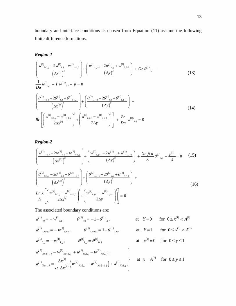
boundary and interface conditions as chosen from Equation (11) assume the following

finite difference formations.

Region-1

( ) ( ) ( )

( )( )

( ) ( ) ( )

( )( )

( ) ( )

1 1 1 1 1 1

1, , 1, , 1 , , 1 1

,2 21

1 1 2

, ,

2 2

10

i j i j i j i j i j i j

i j

i j i j

w w w w w wGr

yx

w I w pDa

+ − + −

− + − +

+ + −

− − =

(13)

( ) ( ) ( )

( )( )

( ) ( ) ( )

( )

( ) ( )

( )

( ) ( )( )

1 1 1 1 1 1

1, , 1, , 1 , , 1

2 21

2 21 1 1 1

1, 1, , 1 , 1 1 2

,1

2 2

022

i j i j i j i j i j i j

i j i j i j i j

i j

yx

w w w w BrBr w

y Dax

+ − + −

+ − + −

− + − +

+ +

− − + + =

(14)

Region-2

( ) ( ) ( )

( )( )

( ) ( ) ( )

( )( )

( )2 2 2 2 2 2 11, , 1, , 1 , , 1 2

,2 22

2 20

i j i j i j i j i j i j

i j

w w w w w w Gr n p

yx

+ − + −

− + − +

+ + − =

(15)

( ) ( ) ( )

( )( )

( ) ( ) ( )

( )

( ) ( )

( )

( ) ( )

2 2 2 2 2 2

1, , 1, , 1 , , 1

2 22

2 22 2 2 2

1, 1, , 1 , 1

2

2 2

022

i j i j i j i j i j i j

i j i j i j i j

yx

w w w wBr

K yx

+ − + −

+ − + −

− + − +

+ +

− − + =

(16)

The associated boundary conditions are:

( ) ( ) ( ) ( ) ( ) ( )1 1 1 1 1 1

,0 ,1 ,0 ,1, 1 , at 0 for 0i i i iw w Y x A = − = − − =

( ) ( ) ( ) ( ) ( ) ( )1 1 1 1 1 1

, 1 , , 1 ,, 1 at 1 for 0i Ny i Ny i Ny i Nyw w Y x A + += − = − =

( ) ( ) ( ) ( ) ( )1 1 1 1 1

0, 1, 1, 0,, at 0 for 0 1j j j jw w x y = − = =

( ) ( ) ( ) ( )

( )( )

( )

( ) ( )( ) ( )

( )

2 1 1 2

2 1, 1, 1, 2,

11

1 2 2 1

1, 2, 2 1, 1,2

,

at for 0 1,

Nx j Nx j Nx j Nx j

Nx j Nx j Nx j Nx j

w w w w

x A yxw w w w

x

+ +

+ +

= + −

= = − +

14

( ) ( ) ( ) ( )

( )( )

( )

( ) ( )( ) ( )

( )

2 1 1 2

2 1, 1, 1, 2,

11

1 2 2 1

1, 2, 2 1, 1,2

,

at for 0 1,

Nx j Nx j Nx j Nx j

Nx j Nx j Nx j Nx j

x A Yx

x

+ +

+ +

= + −

= = − +

( ) ( ) ( ) ( ) ( ) ( ) ( )2 2 2 2 1 2 2

,0 ,1 ,0 ,1, 1 , at 0 fori i i iw w y A x A = − = − − =

( ) ( ) ( ) ( ) ( ) ( ) ( )2 2 2 2 1 2 2

, 1 , , 1 ,, 1 at 0 fori Ny i Ny i Ny i Nyw w y A x A + += − = − =

( ) ( ) ( ) ( ) ( ) ( )2 2 2 2 1 2

0, 1, 1, 0,, at for 0 1j j j jw w x A A y = − = = +

(17)

The difference equations as given in Equations (12) to (16) along with boundary and

interface conditions as given in Equation (17) are iterated incorporating the Southwell-

Over-Relaxation method (ORM). The iteration is carried out until the tolerance value is

achieved. The tolerance value is fixed as 810−. The validation of the code is carried out

in two ways as follows:

1. Grid independence study: Table-1 provides the value of average Nusselt number at

the left wall of the conduit for different sizes of grids. This table infers that the grid sizes

101x101 or 201x201 do not show any noticeable changes in the solutions. That is to say

that the solutions obtained using 101x101 and 201x201 agree very well, hence choosing

either 101x101 or 201x201 does not alter the flow structure i.e. grid independence is

achieved. Hence the 101x101 grid size is adapted for the computations.

2. Validation of the code with previous studies: The results obtained in the present

code are compared with Umavathi and Bég (2020) in the absence of porous material.

The validation of the code in Umavathi and Bég (2020) is carried in detail by comparing

with Oztop et al. (2009) for a composite system, Moshkin (2002) for a two-layer system

in an enclosure and Davis (1963, 1983). Therefore, the present FDM solutions concur

with Umavathi and Bég (2020) in the absence of a porous matrix for pure viscous

immiscible fluids. Table-2 provides the values of average Nusselt number at the left

plate for composite porous medium and viscous immiscible fluids (Umavathi and Bég,

2020). This table indicates that for large Grashof number, Nusselt number is less in

Region-1 in comparison with Region-2. Further the Nusselt number for clear viscous

fluid (Region-2) is close to Umavathi and Bég, (2020). One should note at this point that,

15

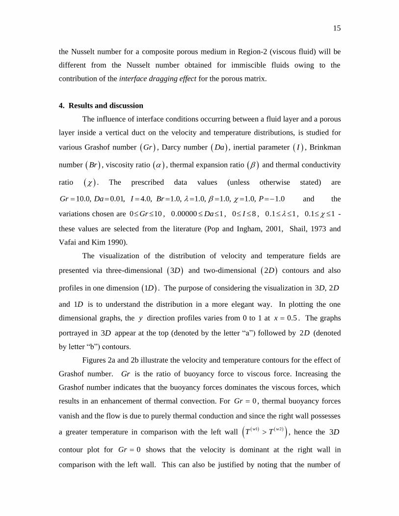
the Nusselt number for a composite porous medium in Region-2 (viscous fluid) will be

different from the Nusselt number obtained for immiscible fluids owing to the

contribution of the interface dragging effect for the porous matrix.

4. Results and discussion

The influence of interface conditions occurring between a fluid layer and a porous

layer inside a vertical duct on the velocity and temperature distributions, is studied for

various Grashof number ( )Gr , Darcy number ( )Da , inertial parameter ( )I , Brinkman

number ( )Br , viscosity ratio ( ) , thermal expansion ratio ( ) and thermal conductivity

ratio ( ) . The prescribed data values (unless otherwise stated) are

10.0, 0.01, 4.0, 1.0, 1.0, 1.0, 1.0, 1.0Gr Da I Br P = = = = = = = =− and the

variations chosen are 0 10Gr , 0.00000 1Da , 0 8I , 0.1 1 , 0.1 1 -

these values are selected from the literature (Pop and Ingham, 2001, Shail, 1973 and

Vafai and Kim 1990).

The visualization of the distribution of velocity and temperature fields are

presented via three-dimensional ( )3D and two-dimensional ( )2D contours and also

profiles in one dimension ( )1D . The purpose of considering the visualization in 3 , 2D D

and 1D is to understand the distribution in a more elegant way. In plotting the one

dimensional graphs, the y direction profiles varies from 0 to 1 at 0.5x = . The graphs

portrayed in 3D appear at the top (denoted by the letter “a”) followed by 2D (denoted

by letter “b”) contours.

Figures 2a and 2b illustrate the velocity and temperature contours for the effect of

Grashof number. Gr is the ratio of buoyancy force to viscous force. Increasing the

Grashof number indicates that the buoyancy forces dominates the viscous forces, which

results in an enhancement of thermal convection. For 0Gr = , thermal buoyancy forces

vanish and the flow is due to purely thermal conduction and since the right wall possesses

a greater temperature in comparison with the left wall ( ) ( )( )1 2w w

T T , hence the 3D

contour plot for 0Gr = shows that the velocity is dominant at the right wall in

comparison with the left wall. This can also be justified by noting that the number of

16

contours are dense at the right wall in comparison with the left wall as seen in the 2D

graph. For 1Gr = , thermal buoyancy and viscous hydrodynamic forces are equal and the

upward direction velocity is more in comparison with the downward direction ( )3D , the

number of contours are less in the lower region ( )0 0.5y in comparison with the

upper region ( )0.5 1y ( )2D . For 0Gr = , there is almost a symmetric distribution

of velocity in the upward and downward directions ( )3D and the number of contours are

equal in both the upper and lower regions ( )2D . The figure 2b indicates that there is no

significant influence of Gr on the temperature distribution for all values of Grashof

number. The temperature distribution is almost linear and symmetric in both the upper

and lower regions. The effect of Gr in Fig. 2c and 2d clearly illustrates that as Gr

increases both the velocity and temperature increase i.e. momentum is assisted as is

thermal diffusion. This is a classical result since as Gr increases, physically the

intensification in thermal convection currents energizes the flow, as noted by Gebhart et

al. (1988).

The enact of Darcy number on the velocity and temperature fields are displayed in

Figs. 3a, b, c, d. As Da increases the velocity increases only in the lower region ( )3D .

Physically small values of Da implies the porous matrix is densely packed (the

permeability is minute), therefore for 0.000001Da= , there is negligible velocity

occurring in the region ( )1

02

ax ( 2D graph shows no contours in this region). The

velocity contours are symmetric for 0.01Da = , 1. However for 0.01Da = , the

contours are flattened in comparison with 1Da = . Furthermore, the number of contours

in the upper region (porous medium) are less in comparison with the lower region (clear

viscous fluid). The impact of Darcy number does not induce any noticeable deviation

and the contours are symmetric with respect to the horizontal symmetric line. The

effective influence of Da is to increase the velocity and also the temperature i.e. to

accelerate the flow and to heat the regime. The enhancement is however more prominent

in velocity (Fig. 3c) in comparison with the temperature (Fig. 3d). The large Darcy

17

number implies a corresponding reduction in friction drag which results in the increase of

velocity in the porous region in comparison with the clear viscous fluid region.

In Figs. 4a, b, c the velocity and temperature distributions for variation of inertial

parameter ( )I are depicted. The 3D graph reveals that the velocity is not significantly

depleted with the inertial drag resistance in the upward and downward directions.

However the shape of the contours in the 2D plot clearly shows that the contours are flat

in region-1 (porous medium) in comparison with the contours in region-2 (clear viscous

fluid). In Figs. 4b and 4c (when magnified) one can identify that the inertial drag

generally reduces both the velocity and temperature fields i.e. it induces flow deceleration

and cooling in the regime.

An increase in Brinkman number manifests in a noticeable increase in the velocity

in both upward and downward directions (Fig. 5a). Figures 5b and 5c when magnified

depict that both velocity and temperature distributions are boosted by enlarging the

Brinkman number. Physically increase in the Brinkman number is associated with

elevation in viscous dissipation effects which causes the increase in temperature and

hence velocity is increased through the buoyancy term.

The effect of viscosity ratio ( )

( )

1

2

=

on the flow field is displayed in Figs. 6a,

b, c. For values of 0.1 = ( ) ( )( )2 1

10 = indicates that the saturated porous medium is

ten times more viscous than the clear fluid, 0.5 = ( ) ( )( )2 1

2 = implies that the

fluid in region-1 is twice as viscous in comparison with the fluid in region-2, 1 =

( ) ( )( )2 1 = implies that the viscosity of the fluid in both regions are equal. In view of

this for 0.1 = , there is almost no flow in region-1, for 0.5 = , the flow is slow in

region-1 and for 1.0 = , the flow is almost equivalent in both the regions. Figure 6a

shows that the flow is accelerated in region-1 as increases ( )3D ; evidently in the 2D

graphs there are no velocity contours in region-1 and relatively few contours for 0.5 =

and significantly more contours for 1.0 = . Figures 6b and 6c clearly reveal that as

increases the velocity and temperature are both suppressed in region -1.

18

The effect of inertial parameter, Brinkman number and viscosity ratio on the

temperature distributions exhibits a similar response for 3D and 2D to that of Grashof

number and hence are excluded for brevity. The effect of thermal conductivity ratio

( )

( )

2

1

K

K

=

is visualized in Figs. 7a, b, c, d. The 3D graphs do not precisely locate

impact of , as the velocity contours resemble each other for all values of . Figure 7b

depicts that the 2D temperature contours are weakly nonlinear for 0.1 = in

comparison with 0.5, 1 = . Figure 7c, d showcase that both the velocity and

temperature decrease as increases. However, the effect of is not substantial on the

velocity field. The impact of and are similar to the impact of these parameters

described in an earlier study by Umavathi and Bég (2020). All the results are drawn

considering equal height and width of the duct (square duct) i.e. the aspect ratio is unity.

The volumetric flow rate, skin friction and average Nusselt number at the left and

right walls of the duct have also been computed and are provided in Tables-3, 4, 5

respectively. The volumetric flow rate increases with higher Grashof number, Darcy

number and Brinkman number whereas it decreases with increment in inertial parameter,

viscosity ratio and conductivity ratio, in both regions. These trends are largely

attributable to the accelerating influence of thermal buoyancy (Grashof number), porous

medium permeability (Darcy number) and viscous dissipation effect (Brinkman number)

and the retarding influence of inertial parameter (second order Forchheimer drag),

viscosity ratio and conductivity ratio. The skin friction at the left wall, dw

dy at 0y = and

at the right wall dw

dy at 1y = for both the regions are given in Table-4. The skin friction

increases for large values of Grashof number, and Darcy number at both duct walls and in

both regions. An upsurge in Brinkman number decreases the skin friction at the left wall

and increases at the right wall for both regions and the converse behavior is induced (i.e.

increasing skin friction at the left wall and reducing skin friction at the right wall) with an

elevation in thermal conductivity ratio. An enhancement in the inertial (Forchheimer)

parameter suppresses the skin friction at both the walls for region-1 and region-2 i.e.

19

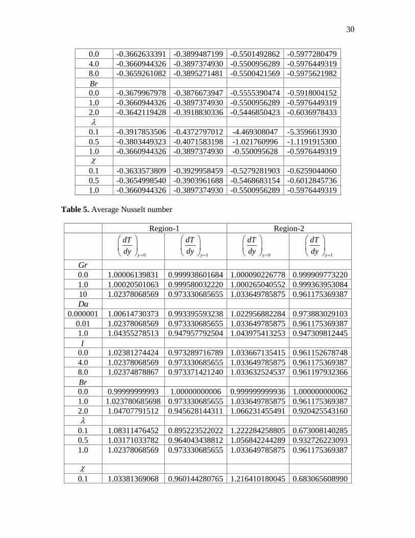
consistently results in flow retardation at the duct boundaries. The average Nusselt

number increases at the left wall and decreases at the right wall with greater magnitudes

of Grashof number, Darcy number and Brinkman number for both duct regions. A rise in

inertial parameter, viscosity ratio and conductivity ratio produce the reverse effect i.e.

they consistently decrease the Nusselt number at the left wall and increase it at the right

wall in both regions of the duct.

5. Conclusions

Motivated by applications in geothermics, thermal insulation and industrial

energy systems, a mathematical model has been developed for the thermally developing

convection flow through a duct of rectangular cross section occupied by composite

porous medium i.e. a fluid layer and porous medium layer. Variable thermophysical

properties have been considered and also viscous heating. The Darcy-Brinkman-

Forchheimer formulation has been implemented. The governing conservation equations

have been rendered non-dimensional with appropriate boundary conditions at the

boundaries and the fluid/porous medium interface. A finite difference method along with

Southwell’s Successive Over Relaxation method has been applied to solve the

transformed nonlinear boundary value problem with appropriate physical data, A grid

(mesh) independence study has been conducted. Validation with earlier studies has also

been included. Extensive visualization of results has been presented for the influence of

the key governing parameters. The present simulations have shown that:

(i)Increasing Grashof, Darcy and Brinkman numbers promotes the velocity while

elevation in inertial parameter, viscosity ratio and thermal conductivity ratio demotes the

velocity.

(ii)The temperature is not significantly modified with any of the governing parameters

except the thermal conductivity ratio.

(iii) The volumetric flow rate is considerably enhanced with higher values of Grashof,

Darcy and Brinkman numbers whereas it is suppressed with greater values of the inertial

(Forchheimer), viscosity ratio and conductivity ratio parameters.

20

(iv) Elevation in Grashof and Darcy numbers increases the skin friction at both walls for

the two regions whereas a rise in Brinkman number (viscous dissipation) decreases the

skin friction at the left wall and increases it at the right wall.

(v) For both the regions the average Nusselt number increases at the left wall and

decreases at the right wall with a boost in Grashof, Darcy and Brinkman numbers. The

opposite trend is computed with an elevation in the inertial parameter, viscosity ratio and

conductivity ratio.

(vi) In the absence of porous matrix the results agree with those computed earlier in

Umavathi and Bég (2020).

The present finite difference and SOR methodology is a versatile approach in immiscible

and porous media thermofluid dynamic analysis. However, the model has assumed the

porous medium to be rigid i.e. non-deformable. Future studies may consider

deformability of the porous medium which is important in thermoelastic geological

systems (boreholes, reservoir formations) and stratified flows and will be communicated

in the near future.

(2a)

21

(2b)

(2c) (2d)

22

0.0 0.2 0.4 0.6 0.8 1.0

-0.04

-0.02

0.00

0.02

0.04

w

x

G r = 0, 1, 10

0.0 0.2 0.4 0.6 0.8 1.0

-0.4

-0.2

0.0

0.2

0.4

G r = 0, 1, 10

10

Gr = 0, 1

x

Figure 2. Velocity (2a, c) and temperature (2b, d) contours and profiles for different Gr

(3a)

(3b)

23

(3c) (3d)

0.0 0.2 0.4 0.6 0.8 1.0-0.08

-0.04

0.00

0.04

0.08

w

x

1

0.01

Da = 0.000001

0.0 0.2 0.4 0.6 0.8 1.0

-0.4

-0.2

0.0

0.2

0.4

1

0.01

Da = 0.000001

Da = 0.000001, 0.01, 1

x

Figure 3. Velocity (3a, c) and temperature (3b, d) contours and profiles for different Da

(4a)

24

(4b) (4c)

0.0 0.2 0.4 0.6 0.8 1.0

-0.04

-0.02

0.00

0.02

0.04

0.06

w

x

I = 0, 4, 8

I = 0, 4, 8

0.0 0.2 0.4 0.6 0.8 1.0

-0.4

-0.2

0.0

0.2

0.4

I = 0, 4, 8

x

I = 0, 4, 8

Figure 4. Velocity (4a, b) and temperature (4c) contours and profiles for different I

25

(5a)

(5b) (5c)

0.0 0.2 0.4 0.6 0.8 1.0

-0.04

-0.02

0.00

0.02

0.04

2

1

Br = 0 . 0

B r = 0, 1, 2

w

x

0.0 0.2 0.4 0.6 0.8 1.0

-0.4

-0.2

0.0

0.2

0.4

2

1

Br = 0

B r = 0, 1, 2

x

Figure 5. Velocity (5a, b) and temperature (5c) contours and profiles for different Br

26

(6a)

(6b) (6c)

0.0 0.2 0.4 0.6 0.8 1.0-0.15

-0.10

-0.05

0.00

0.05

0.10

0.15

w

x

= 0.1, 0.5, 1

0.0 0.2 0.4 0.6 0.8 1.0

-0.4

-0.2

0.0

0.2

0.4

x

= 0.1, 0.5, 1

10.5

= 0.1

Figure 6. Velocity (6a, b) and temperature (6c) contours and profiles for different

27

(7a)

(7b)

28

(7c) (7d)

0.0 0.2 0.4 0.6 0.8 1.0

-0.04

-0.02

0.00

0.02

0.04

= 0.1, 0.5, 1

0.5, 1

= 0.1

w

x

0.0 0.2 0.4 0.6 0.8 1.0

-0.4

-0.2

0.0

0.2

0.4

x

= 0.1, 0.5, 1

1

0.5

= 0.1

Figure 7. Velocity (7a, c) and temperature (7b, d) contours and profiles for different

Table 1. Grid independence test

Size of the grid Region-1 Region-2

11 11 1.02405361854933 1.03226665365408

51 51 1.02377669154082 1.03360202945089

101 101 1.02378068569846 1.03364978587588

151 151 1.02378158702730 1.03365869051294

201 201 1.02378191542428 1.03366181226918

Table 2. Comparison for Pr 1, 0.1, 1, 1, 1Br Ec P = = = = − = = =

Present ( )1, 4Da I= = Umavathi and Bég (2020)

( )0, 0Da I= =

Gr Region-1 Region-2 Region-1 Region-2

1 1.0003734744657 1.0003748511311 1.0003783577697 1.0003783577697

10 1.0435527851379 1.0439754132530 1.0444145000752 1.0444145000752

20 1.1656069078517 1.1676634911878 1.1699171414455 1.1699171414455

29

Table 3. Volumetric flow rate

Volumetric Flow Rate

Region-1 Region-2

Gr

0.0 0.000850282128275056 0.002184807922801564

1.0 0.000850639868417865 0.002186145002066430

10 0.001202846270591417 0.003243189801734679

Da

0.000001 0.000000015729500906 0.001925163167817541

0.01 0.001202846270591417 0.003243189801734679

1.0 0.005661138851524346 0.005826400327368434

I

0.0 0.001205630197327104 0.003245643130821721

4.0 0.001202846270591417 0.003243189801734679

8.0 0.001200081904799690 0.003240752368332471

Br

0.0 0.000848684101737182 0.002183737570140714

1.0 0.001202846270591417 0.003243189801734679

2.0 0.001562484200892853 0.004319849760333960

0.1 0.003183676864360223 0.070585858124905310

0.5 0.001466473122143211 0.006736670074203001

1.0 0.001202846270591417 0.003243189801734679

0.1 0.001780004089626783 0.007766538485297454

0.5 0.001323353533740122 0.003870810823821523

1.0 0.001202846270591417 0.003243189801734679

Table 4. Skin friction

Region-1 Region-2

0y

dw

dy=

1y

dw

dy=

0y

dw

dy=

1y

dw

dy=

Gr

0.0 0.0098488530 -0.0098488530 0.0181377773 -0.0181377773

1.0 -0.0279502789 -0.0476509280 -0.0392296607 -0.0755190287

10 -0.3660944326 -0.3897374930 -0.5500956289 -0.5976449319

Da

0.000001 -0.0000989799 -0.0001031051 -0.4630514858 -0.4957047084

0.01 -0.3660944326 -0.3897374930 -0.5500956289 -0.5976449319

1.0 -0.5960329782 -0.6678486590 -0.6012725456 -0.6749302692

I

30

0.0 -0.3662633391 -0.3899487199 -0.5501492862 -0.5977280479

4.0 -0.3660944326 -0.3897374930 -0.5500956289 -0.5976449319

8.0 -0.3659261082 -0.3895271481 -0.5500421569 -0.5975621982

Br

0.0 -0.3679967978 -0.3876673947 -0.5555390474 -0.5918004152

1.0 -0.3660944326 -0.3897374930 -0.5500956289 -0.5976449319

2.0 -0.3642119428 -0.3918830336 -0.5446850423 -0.6036978433

0.1 -0.3917853506 -0.4372797012 -4.469308047 -5.3596613930

0.5 -0.3803449323 -0.4071583198 -1.021760996 -1.1191915300

1.0 -0.3660944326 -0.3897374930 -0.550095628 -0.5976449319

0.1 -0.3633573809 -0.3929958459 -0.5279281903 -0.6259044060

0.5 -0.3654998540 -0.3903961688 -0.5468683154 -0.6012845736

1.0 -0.3660944326 -0.3897374930 -0.5500956289 -0.5976449319

Table 5. Average Nusselt number

Region-1 Region-2

0y

dT

dy=

1y

dT

dy=

0y

dT

dy=

1y

dT

dy=

Gr

0.0 1.00006139831 0.999938601684 1.000090226778 0.999909773220

1.0 1.00020501063 0.999580032220 1.000265040552 0.999363953084

10 1.02378068569 0.973330685655 1.033649785875 0.961175369387

Da

0.000001 1.00614730373 0.993395593238 1.022956882284 0.973883029103

0.01 1.02378068569 0.973330685655 1.033649785875 0.961175369387

1.0 1.04355278513 0.947957792504 1.043975413253 0.947309812445

I

0.0 1.02381274424 0.973289716789 1.033667135415 0.961152678748

4.0 1.02378068569 0.973330685655 1.033649785875 0.961175369387

8.0 1.02374878867 0.973371421240 1.033632524537 0.961197932366

Br

0.0 0.99999999993 1.00000000006 0.999999999936 1.000000000062

1.0 1.023780685698 0.973330685655 1.033649785875 0.961175369387

2.0 1.04707791512 0.945628144311 1.066231455491 0.920425543160

0.1 1.08311476452 0.895223522022 1.222284258805 0.673008140285

0.5 1.03171033782 0.964043438812 1.056842244289 0.932726223093

1.0 1.02378068569 0.973330685655

1.033649785875 0.961175369387

0.1 1.03381369068 0.960144280765 1.216410180045 0.683065608990

31

0.5 1.02784478571 0.968592747828 1.058360368768 0.930316538235

1.0 1.02378068569 0.973330685655 1.033649785875 0.961175369387

Conflict of interest: The authors do not have any conflict of interest

Acknowledgements

Both authors are grateful to the reviewers for their astute comments which have served to

improve the article and furthermore have identified interesting future directions for

simulations.

References

Alzami, B. and Vafai, K. (2001), “Analysis of fluid flow and heat transfer

interfacial conditions between a porous medium and a fluid layer”, Int. J. Heat

and Mass Transfer, Vol. 44, pp. 1735-1749.

Amiri, A. and Vafai, K. (1995), “Effects of boundary conditions on non-Darcian

heat transfer through porous media and experimental comparisons”,

Num Heat Transfer, Vol. 27, pp. 651-664.

Amiri, A. and Vafai, K. (1994), “Analysis of dispersion effects and non-thermal

equilibrium, non-Darcian, variable-porosity incompressible flow through porous

Media”, Int. J. Heat Mass Transfer, Vol. 37, pp. 939-954.

Arquis, E. and Caltagirone, J.P. (1987), “Interacting convection between fluid and open

porous layers”, ASME paper No. 87-WA/HT-24.

Arzhang, K., Shivakumara, I.S. and Suma, S.P., (2003), “Convective instability in

superposed fluid and porous layers with vertical through flow”, Transport in

Porous Media, Vol. 51, pp. 1–18.

Bagchi, A. and Kulacki, F.A., (2020), “Natural convection in superposed fluid-porous

layers”, Springer Briefs in Thermal Engineering and Applied Science, Springer

Nature.

Baytas, A.C. and Pop, I. (1999), “Free convection in oblique enclosures filled

with a porous medium”, Int. J. Heat Mass Transfer, Vol. 42, pp. 1047–1057.

Beckermann, C., Viskanta, R. and Ramadhyani, S. (1987), “Natural convection flow

and heat transfer between a fluid layer and a porous layer inside a

32

rectangular enclosure, ASME J. Heat Transfer, Vol. 109, pp. 363-370.

Beckermann, C., Viskanta, R. and Ramadhyani, S. (1986), “A numerical study of non-

Darcian natural convection in a vertical enclosure filled with a porous medium”,

Numer. Heat Transfer, Vol.10, pp. 557-570.

Bevers, G. and Joseph, D.D. (1967), “Boundary conditions at a naturally permeable

wall”, J. Fluid Mech., Vol. 30, pp. 197-207.

Borrelli, A., Giantesio, G. and Patria, M.C. (2017), “ Reverse flow in magnetoconvection

of two immiscible fluids in a vertical channel”, ASME J. Fluids Eng., Vol. 139,

pp. 101203 (16 pages).

Campos, H., Morales, J.C., Lacoa, U. and Campo, A. (1990), “Thermal aspects of a

vertical annular enclosure divided into a fluid region and a porous region, Int.

Comm. Heat Mass Transfer, Vol. 17, pp. 343-354.

Chikh, S., Boumedian, A., Bouhadef, K. and Lauriat, G. (1995), “Analytical solution of

non-Darcian forced convection in an annular duct partially filled with

porous medium, Int. J. Heat Mass Transfer, Vol. 38, pp. 1543-1551.

Christian, G. and Fryer, P. (2006), “The effect of pulsing cleaning chemicals on the

cleaning of whey protein deposits”, Food Bioprod. Process., Vol. 84,

pp. 320–328.

Cole, P., Asteriadou, K., Robbins, P., Owen, E., Montague, G. and Fryer, P. (2010),

“Comparison of cleaning of toothpaste from surfaces and pilot scale pipe work”,

Food Bioprod. Process., Vol. 88, pp. 392–400.

De Vahl Davis, G. (1968), “Laminar natural convection in an enclosed rectangular

cavity” , Int. J. Heat Mass Transfer, Vol. 11, pp.167–1693.

De Vahl Davis, G. (1983), “Natural convection of air in a square cavity”, Int. J. Num.

Meth. Fluids, Vol. 3, pp. 249-264.

Du, Z.G. and Bilen, E. (1990), “Natural convection in vertical cavities with partially

filled heat-generating porous medium”, Numerical Heat Transfer, Vol. 18A,

pp. 371-386.

Howell, P., Waters, S. and Grotberg, J. (2000), “The propagation of a liquid bolus along

a liquid-lined flexible tube”, J. Fluid Mech., Vol. 406, pp. 309–335.

Hulin, J., Znaien, J., Mendonca, L., Sourbier, A., Moisy, F., Salin, D. and Hinch, E.,

33

(2008), “Buoyancy driven interpenetration of immiscible fluids of different

densities in a tilted tube”, in APS Division of Fluid Dynamics (American Physical

Society), Vol. 1.

Jaluria, Y. and Gebhart, B. (1988), Buoyancy-induced Flows and Transport, Hemisphere,

Washington, USA.

Jones, M. C. and Persichetti, J. M. (1986), “Convective instability in packed beds”,

AIChemE J., Vol. 32, pp. 1555–1557.

Kapur, J.N. and Shukla, J.B. (1964), “The flow of incompressible immiscible fluids

between two plates”, Appl. Sci. Res., Vol. 13, pp. 55-60.

Kaviany, K. (1991), Principles of Heat transfer in Porous Media, Springer-Verlag,

New York.

Kaviany, M. (1985), “Laminar flow through a porous channel bounded by

isothermal parallel plates”, Int. J. Heat Mass Transfer, Vol. 28, pp. 851-858.

Kim, S.J. and Choi, C.Y. (1996), “Convection heat transfer in porous and overlying

layers heated from below”, Int. J. Heat Mass Transfer, Vol. 39, pp. 319-329.

Kim, S.Y., Kang, B.H. and Hyuan, J. M. (1994), “Heat transfer from pulsating flow in a

Channel filled with porous media”, Int. J. Heat Mass Transfer, Vol. 37,

pp. 2025-2033.

Kuznetsov, A.V., (1999), “A boundary layer solution for the momentum and energy

transport in the interface region between a porous medium and a fluid layer”, 33rd

National Heat Transfer Conference NHTC'99, Albuquerque, NM (USA),

08/15/1999--08/17/1999.

Lewis, R.W. and Nithiarasu, P. and Seetharamu, K.N., (2004), Fundamentals of the

Finite Element Method for Heat and Fluid Flow, John Wiley and Sons, New York, USA.

Lewis, R.W. and Schrefler, B.A. (1998), The Finite Element Method In The Static

and Dynamic Deformation and Consolidation of Porous Media, John Wiley and Sons,

New York, USA.

Liu, I.C., Umavathi, J.C. and Wang, H.H. (2012), “Poiseuille-Couette flow and heat

transfer in an inclined composite porous medium”, J. of Mechanics.,

Vol. 28, pp. 559-566.

Malashetty, M.S., Umavathi, J.C. and Prathap Kumar, J. (2004), “Two fluid flow and

34

heat transfer in an inclined channel containing porous and fluid layer, Heat

and Mass Transfer, Vol. 40, pp. 871-876.

Malashetty, M.S., Umavathi, J.C. and Prathap Kumar, J. (2005), “Flow and heat transfer

in an inclined channel containing a fluid layer sandwiched between two

porous layers”, Journal of Porous Media, Vol. 8, pp. 443-453.

Malashetty, M.S., Umavathi, J.C. and Prathap Kumar, J.: 2001, Convective flow and heat

transfer in a composite porous medium, Journal of Porous Media, 4, 15-22.

Manole, D.M. and Lage, J.L. (1992), “Numerical benchmark results for natural

convection in a porous medium cavity”, HTD, Heat and Mass Transfer in

Porous Media, ASME Conference, Vol. 216, pp. 55-60.

Manu, C., Sabino, S., Iman, A., Mark, J.M., Chris, R.K. and Sasa, K. (2020), “Effect of

packing height and location of porous media on heat transfer in a cubical cavity:

Are extended Darcy simulations sufficient?”, Int. J. Heat and Fluid Flow, Vol. 84,

pp. 108617 (12 pages).

Min, J.Y. and Kim, S.J., (2005), “A novel methodology for thermal analysis of a

composite system consisting of a porous medium and an adjacent fluid layer”,

ASME J. Heat Transfer, Vol. 127, pp. 648-656.

Mohamad, C. , Yousef, H and Bernd, M. (2020), “Upscaling LBM-TPM simulation

approach of Darcy and non-Darcy fluid flow in deformable, heterogeneous porous

media”, Int. J. Heat and Fluid Flow, Vol. 83, pp. 108566 (13 pages).

Moshkin, N.P. (2002), “Numerical model to study natural convection in a rectangular

enclosure filled with two immiscible fluids”, Int. J. Heat and Fluid Flow,

Vol. 23, pp. 373-379.

Neale, G. and Nader, W. (1974), “Practical significance of Brinkman’s extension

of Darcy’s law: coupled parallel flows within a channel and a bounding

porous Medium” , Can. J. Chem. Engng., Vol. 52, pp. 475-478.

Nield, D.A. and Bejan, A. (1999), Convection in Porous Media, Second ed., Springer-

Verlag, New York.

Nithiarasu, P., Lewis, R.W. and Seetharamu, K.N. (2015), Fundamentals of the Finite

Element Method for Heat and Mass Transfer, Second Edition, Wiley.

Oztop, H.F., Yasin Varol, Ahmet Koca, (2009), “Natural convection in a vertically

35

divided square enclosure by a solid partition into air and water regions”, Int. J.

Heat and Mass Transfer, Vol. 52, pp. 5909-5921.

Pop, I. and Ingham, D.B., (2001), Convective Heat Transfer: Mathematical and

Computational Modeling of Viscous Fluids and Porous Media, Elsevier Science

& Technology Books, The Netherlands.

Prasad, V. (1990), “Convection flow interaction and heat transfer between fluid and

porous layers”, Proc. NATO Advanced Study Institute on Convective Heat and

Mass Transfer in Porous Media, Turkey.

Prasad, V. and Kulacki, F.A. (1984), “Convective heat transfer in a rectangular porous

cavity-effect of aspect ratio on flow structure and heat transfer”, ASME J. Heat

Transfer, Vol. 106, pp. 158-165.

Redapangu, P., Vanka, S. and Sahu, K. (2012), “Multiphase lattice Boltzmann

simulations of buoyancy-induced flow of two immiscible fluids with different

viscosities”, Eur. J. Mech.-B Fluids, Vol. 34, pp. 105–114.

Regner, M., Henningsson, M., Wiklund, J., O¨ stergren, K. and Tragardh, C. (2007),

“Predicting the displacement of yoghurt by water in a pipe using CFD”, Chem.

Eng. Technol., Vol. 30, pp. 844–853.

Sahu, K. and Vanka, S. (2011), “A multiphase lattice Boltzmann study of buoyancy

induced mixing in a tilted channel”, Comput. Fluids, Vol. 50, pp. 199–215.

Shail, R. (1973), “On laminar two-phase flow in magneto hydrodynamics”, Int. J. Eng.

Sci., Vol. 11, pp. 1103–1108.

Song, M. and Viskanta, R. (1994), “Natural convection flow and heat transfer within

a rectangular enclosure containing a vertical porous layer”, Int. J. Heat

MassTransfer, Vol. 37, pp. 2425-2438.

Sozen, M. and Kuzay, T.M. (1996), “Enhanced heat transfer in round tubes with porous

inserts”, Int. J. Heat Fluid Flow, Vol. 17, pp. 124-129.

Srinivas, J. and Ramana Murthy, J.V. (2016a), “Flow of two immiscible couple stress

fluids between two permeable beds”, J. Appl. Fluid Mech., Vol. 9, pp. 501-507.

Srinivas, J. and Ramana Murthy, J.V., (2016b), “Second law analysis of the flow of two

immiscible micropolar fluids between two porous beds”, J. Eng. Thermophys,

Vol. 25, pp. 126 -142.

36

Srinivasan, V. and Vafai, K. (1994), “Analysis of linear encroachment in two immiscible

fluid systems in a porous medium”, ASME J. Fluids Eng., Vol. 116, pp. 135-139.

Tien, C.L. and Vafai, K. (1989), “Convective and radiative heat transfer in porous

media”, Advances in Appl. Mech., Vol. 27, pp. 225-281.

Umavathi, J.C. and Bég, O.A., (2020), “Effects of thermo physical properties on heat

transfer at the interface of two immiscible fluids in a vertical duct: Numerical

study”, Int. J. of Heat and Mass Transfer, Vol. 154, pp.119613 (18 pages)

Umavathi, J.C. and Santosh, V. (2012a), “Non-Darcy mixed convection in a vertical

porous channel with boundary conditions of third kind”, Trans. Porous Media,

Vol. 95, pp. 111-131.

Umavathi, J.C. and Shekar, M. (2014), “Mixed convective flow of immiscible fluids in

a vertical corrugated channel with traveling thermal waves”, J. King Saud

University- Engineering Sciences, Vol. 26, pp. 49-68.

Umavathi, J.C. and Sheremet, M. (2019), “Flow and heat transfer of couple stress

nanofluid sandwiched between viscous fluids”, Int. J. Numerical Methods for

Heat and Fluid Flow, Vol. 29, pp. 4262-4276.

Umavathi, J.C., (2013), “Analysis of flow and heat transfer in a vertical rectangular duct

using a non-Darcy model”, Trans. Porous Media, Vol. 96, pp. 527–545.

Umavathi, J.C., (2015a), “Free convective flow in a vertical rectangular duct filled with

porous matrix for viscosity and conductivity variable properties”, Int. J.

Heat and Mass Transfer, Vol. 81, 383-403.

Umavathi, J.C., (2015b), “Combined effect of variable viscosity and variable

thermal conductivity on double diffusive convection flow of a permeable

fluid in a vertical channel”, Trans. Porous Media, Vol. 108, pp. 659-678.

Umavathi, J.C., Chamkha, A.J. and Sridhar, K.S.R., (2010), “Generalised plain Couette

flow heat transfer in a composite channel, Trans. Porous Media, Vol. 85,

pp. 157-169.

Umavathi, J.C., Chamkha, A.J., Mateen, A. and Al-Mudhaf, A. (2005), “Unsteady two

fluid flow and heat transfer in a horizontal channel”, Heat Mass Transfer, Vol.

42, pp. 81-90.

Umavathi, J.C., Malashetty, M.S. and Mateen, A. (2004), “Fully developed flow and heat

37

transfer in a horizontal channel containing an electrically conducting fluid

sandwiched between two fluid layers”, Int. J. Applied Mechanics and Eng., Vol.

9, pp. 781-794.

Umavathi, J.C., Prathap Kumar, J. and Jaweriya, S. (2012b), “Mixed convection flow in

a vertical porous channel with boundary conditions of third kind with heat

source/sink”, J. Porous Media, Vol. 15, pp. 998-1007.

Umavathi, J.C., Shaik Meera, D. and Liu, I.C., (2008), “Unsteady flow and heat transfer

of three immiscible fluids”, Int. J. Appl. Mech. Engg., Vol. 13, pp. 1079-1100.

Vafai, K. (2000), Handbook of Porous Media, Marcel Dekker, New York.

Vafai, K. and Kim, S. (1989), “Forced convection in a channel filled with porous

medium: and exact solution”, ASME J. Heat Transfer, Vol. 111, pp. 1103-1106.

Vafai, K. and Kim, S.J. (1990), “Fluid mechanics of the interface region between a

porous medium and a fluid layer-an exact solution”, Int. J. Heat Fluid Flow,

Vol. 11, pp. 254-256.

Vafai, K. and Thiyagaraja, R. (1987), “Analysis of flow and heat transfer at the

interface region of a porous medium”, Int. J. Heat Mass Transfer, Vol. 30,

pp. 1391-1405.

Valette, R., Laure, P., Demay, Y. and Agassant, J. (2004), “Convective linear stability

analysis of two-layer co extrusion flow for molten polymers, J. Non-Newtonian

Fluid Mech., Vol. 121, pp. 41–53.