Department of Applied Mathematics, University of Venice WORKING PAPER SERIES Shira Fano, Marco Li Calzi, Paolo Pellizzari Convergence of outcomes and evolution of strategic behavior in double auctions Working Paper n. 196/2010 February 2010 ISSN: 1828-6887
Transcript
Department of Applied Mathematics, University of Venice
WORKING PAPER SERIES
Shira Fano, Marco Li Calzi, Paolo Pellizzari
Convergence of outcomes and
evolution of strategic behavior in
double auctions
Working Paper n. 196/2010
February 2010
ISSN: 1828-6887
This Working Paper is published under the auspices of the Department of Applied
Mathematics of the Ca’ Foscari University of Venice. Opinions expressed herein are
those of the authors and not those of the Department. The Working Paper series is
designed to divulge preliminary or incomplete work, circulated to favour discussion
and comments. Citation of this paper should consider its provisional nature.
Dept. Applied Mathematics Dept. Applied Mathematics and Dept. Applied Mathematics and
University of Venice Advanced School of Economics, Advanced School of Economics,
University of Venice University of Venice
(February 2010)
Abstract. We study the emergence of strategic behavior in double auctions with an equalnumber n of buyers and sellers, under the distinct assumptions that orders are cleared simul-taneously or asynchronously. The evolution of strategic behavior is modeled as a learningprocess driven by a genetic algorithm. We find that, as the size n of the market grows,allocative inefficiency tends to zero and performance converges to the competitive outcome,regardless of the order-clearing rule.
The main result concerns the evolution of strategic behavior. Under simultaneous order-clearing, as n increases, only marginal traders learn to be price takers and make offers equal totheir valuations/costs. Under asynchronous order-clearing, as n increases, all intramarginaltraders learn to be price makers and make offers equal to the competitive equilibrium price.The nature of the order-clearing rule affects in a fundamental way what kind of strategicbehavior we should expect to emerge.
∗ We thank the audience of the workshop on “Evolution and market behavior in economics and finance” heldat the Scuola Superiore Sant’Anna for their comments. The second and third author acknowledge financialsupport from MIUR under grants 2007EENEAX and 2007TKLTSR.
1 Introduction
The double auction institution encompasses different families of trading protocols that gatherbuyers and sellers in a single exchange market; see Friedman (1993). The two prominentinstances are the call market and the continuous double auction, that differ in whetherorders are cleared simultaneously or asynchronously. Both kinds of protocols have beenwidely studied with a three-pronged approach based on analytical derivations, laboratory orfield experiments, and computer simulations.
While the k-double auction has emerged as the standard model for the call market, thereis no dominant paradigm for the continuous double auction. The sheer number of possiblevariants impairs the emergence of a single representative format. There is a vast literaturescattered over different formulations, using a devilish variety of assumptions on the richnessof the strategy space. This may depend on information as diverse as the past history of ordersor transactions, the current status of the book, the timing at which an offer is made, andanother myriad of protocolary details such as the option to cancel and resubmit orders or theobligation to submit price-improving offers (a.k.a. as “NYSE spread-improvement rule”). Inorder to make progress, it is necessary to give up on generality.
We study a simple model for the double auction where the strategies of the tradersdepend only on their private types. This simplification allows to provide a unified modelfor the k-double auction and the continuous double auction, where the only difference isin the order-clearing rule. For the special case where the market has only one buyer andone seller, we prove that the equilibrium strategies coincide but the equilibrium outcome isdifferent. This provides a sharp illustration of the direct effects of the order-clearing rule onthe performance of a trading protocol.
Our main objective is the study of which trading strategies emerge as strategically plau-sible when the number of traders increases. This plausibility encompasses two requirements:the profile of strategies must be (close to) an equilibrium and it must be the outcome ofan evolutionary process (e.g., learning) that justifies its prominence. (In other words, wedo not assume that “all equilibria are created equal”.) Our approach is to let agents usegenetic algorithms to maximize individual profits and coevolve a profile of (possibly random-ized) trading strategies. This evolutionary approach circumvents many of the computationaldifficulties that affects the search for equilibrium strategies in current models of continuousdouble auctions.
In the long run, as evolution takes place, we show that agents learn to (approximately)play equilibrium strategies. Our first result is consistent with the asymptotic approach tothe “equivalence principle” (see Aumann, 1987), according to which increasing the number ofagents diminishes their strategic influence and lead the system towards the competitive out-come. Regardless of the order-clearing rule, as the market grows in size, allocative inefficiencytends to zero and performance converges to the competitive outcome. For the k-double auc-tion, this result is magisterially exemplified in Rustichini et al. (1994) that proves the strongerstatement that traders’ equilibrium offers asymptotically converges to truth-telling: they arewilling to accept any price below (above) their valuations (costs) so they act as perfectlycompetitive price-takers.
Our main results concern the evolution of strategic behavior when the market grows in
1
size. In a nutshell, we show that the asymptotic emergence of the competitive outcome doesnot imply that all traders should learn to be price takers. Moreover, the order-clearing ruleaffects in a fundamental way what kind of strategic behavior we should expect to emerge.Under simultaneous order-clearing, as n increases, only marginal traders learn to be pricetakers and make offers equal to their valuations/costs. This implies that the asymptoticallyunique equilibrium strategies derived in Rustichini et al. (1994) are unlikely to be learnable.Under asynchronous order-clearing, as n increases, all intramarginal traders learn to be pricemakers and make offers equal to the competitive equilibrium price.
There is a growing literature on the application of evolutionary processes to the studyof market protocols and trading strategies. MacKie-Mason and Wellman (2006) provides asurvey centered around the general field of computational market design, where both protocolsand strategies may be allowed to change. This paper exploits genetic algorithms to evolveand compare strategic behavior across two specific formats for the double auction. To thebest of our knowledge, Dawid (1999) is the first explicit application of genetic algorithms forthe derivation of strategic behavior in a double auction market. Phelps et al. (2006) providesan evolutionary comparison between three families of strategies: it concludes that, as themarket grows in size, truth-telling becomes increasingly likely to emerge in a call marketwhile it tends to disappear in a continuous double auction. Anufriev et al. (2010) applies analgorithm known as individual evolutionary learning to study the effects of public disclosureof information on the evolution of strategic behavior in a continuous double auction.
Our paper is organized as follows. Section 2 presents a unified model for the k-doubleauction and the continuous double auction, considered as games with incomplete informationwhere traders’ strategies depend only on their private types but different order-clearing rulesapply. Section 3 describes in detail the setup for our simulations. Section 4 collects ourresults on the asymptotic emergence of outcome and strategic behavior for the k-doubleauction, when order-clearing is simultaneous. Section 5 reviews and contrasts the analogousresults for the continuous double auction, when order-clearing is asynchronous. Section 6provides an additional comparative analysis between the strategies evolved by our geneticalgorithm for the continuous double auction against the current benchmark in the literature,as provided by Zhan and Friedman (2007). An appendix collects spurious material.
2 A unified model
There are many variants of the double auction; see Friedman (1993). We focus on whetherorders are cleared simultaneously or asynchronously. The first case characterizes the class oftrading protocols known as call markets or batch auctions. The second case characterizes thefamily of the continuous double auctions. We study a model that encompasses both clearingrules and make it simple to elucidate their effects on the asymptotic convergence of outcomesand the emergence of strategic behavior.
The presentation is organized as follows. The environment described in Section 2.1 collectsthe general characteristics of the economy, including agents’ preferences and endowments.Section 2.2 summarizes the well-known model of a k-double auction for the call market andreviews its main properties. For our purposes, its most important feature is that it is assumes
2
a simple strategy space for each trader. Section 2.3 describes our own model for a continuousdouble auction. We impose assumptions that make the strategy space of each trader as simpleas in the k-double auction. Analogous simplifications underlie other models of the continuousdouble auction, ranging from the nonstrategic (e.g., Gode and Sunder, 1993) to the strategicones (e.g., Zhan and Friedman, 2007). Section A in the appendix discusses a special caseknown as the bilateral trading model with one buyer and one seller, which provides a commonfoundation for the k-double auction and our version of the continuous double auction.
2.1 The environment
There is an equal number n of buyers and sellers. All traders wish to maximize expectedprofits. Each of them is in the market to exchange at most one unit of a generic good per day.Each buyer i has a private valuation vi and each seller j has a private cost cj . Valuationsand costs are drawn from two (stochastically independent, as well as atomless and absolutelycontinuous) distributions F and G over the same support, which we normalize to [0, 1] withoutloss of generality. As a special case, it is customary to assume that F and G are uniformdistributions on [0, 1].
When all traders are price takers, it is customary to define intramarginal and extra-marginal buyers (sellers) depending on their position on the demand (supply) function withrespect to the market-clearing price(s). We follow tradition but refine this qualitative dis-tinction into a complete ordering. Define the strength of a buyer with valuation v as thedistance from the valuation of the weakest buyer (v = 0) and the strength of a seller withcost c as the distance from the valuation of the weakest seller (c = 1). Stronger traders havevaluations (or costs) lying farther away from the market-clearing price(s).
2.2 Simultaneous order clearing
The standard model for a call market where orders are cleared simultaneously is the k-doubleauction; see Satterthwaite and Williams (1993). Buyers and sellers are required to submitprice offers simultaneously. Each buyer declares the maximum bid price at which he is willingto buy and each seller issues the minimum ask price at which she is willing to sell. Tradersdecide strategically their price offers to maximize their expected payoffs. The strategy of abuyer i is a bidding function βi : [0, 1]→ R+ that defines his bid bi = βi(vi) as a function ofhis valuation vi. Similarly, the strategy of a seller j is an asking function αj : [0, 1] → R+
that defines his ask aj = αj(cj) as a function of her cost cj .Buyers’ and sellers’ offers are aggregated to form the demand and supply functions. Their
intersection defines an interval [p1, p2] of market-clearing prices. The k-double auction selectsas trading price the value p∗ = (1 − k)p1 + kp2, where each choice of k in [0, 1] defines adifferent mechanism. Trade occurs among buyers who bid no less than p∗ and sellers whoask no more than p∗. (Some rationing may take place at the margin, but the exact detailsare not relevant.) When a transaction takes place at price p between a buyer with valuationv and a seller with cost c, the payoffs are v − p and p − c respectively. If he does not enterinto a transaction, the payoff for the trader is zero.
As discussed in Leininger et al. (1989), there exist infinitely many Bayes-Nash equilibria
3
for the k-double auction, but two important families have been singled out. The first classcollects the equilibria where the strategies satisfy a pair of differential equations; the secondclass is formed by the equilibria where the strategies are step functions. The literature usuallyrestricts attention to the subset of symmetric1 equilibria in the first class, where all buyersuse the same (differentiable) bidding function β and all sellers use the same (differentiable)asking function α. This simplifies the specification of a profile of equilibrium strategies for nbuyers and n sellers to a single pair (β, α).
We say that the symmetric strategy profile (β, α) is nontrivial if: 1) traders never play(weakly) dominated strategies; that is, β(v) ≤ v and α(c) ≥ c; 2) the set of buyers biddingb > 0 and the set of seller asking a < 1 have strictly positive probability. The first requirementupholds individual rationality : a buyer never bids above his value and a seller never asks belowher cost. The second requirement rules out “no-trade” equilibria. The general features of anontrivial symmetric and differentiable equilibrium of the k-double auction are stated in awell-known result from Rustichini et al. (1994).
Theorem 1 For any nontrivial symmetric and differentiable equilibrium (β, α):
1) there exist values v∗ < 1 and c∗ > 0 such that a buyer with valuation v trades withpositive probability if and only if v > v∗ and a seller with cost c trades with positiveprobability if and only if c < c∗;
2) β and α are increasing over (v∗, 1] and [0, c∗), respectively;
The intervals (v∗, 1] and [0, c∗] define the domain of serious offers where the bidding andasking functions are uniquely defined. We call serious buyers (sellers) those traders who aresupposed to make serious bids (asks) in equilibrium.
For a given value n, in any symmetric and differential equilibrium serious buyers shadetheir valuations and bid β(v) < v; similarly, serious sellers markup their costs and askα(c) > c. This misrepresentation marks a departure from naive price-taking behavior andoccurs as a result of the strategic interaction between all traders. Intuitively, when n getslarge, one expect the scope for strategic misrepresentation to shrink so that the equilibriumprice should tend towards the competitive value. This is formally shown in Rustichini et al.(1994) who prove that, as n ↑ ∞, in any nontrivial symmetric and differentiable equilibriumthe amount of strategic misrepresentation |v− β(v)|+ |α(c)− c| drops to zero as O(1/n) andthe allocative inefficiency disappears at a rate O(1/n2). Satterthwaite and Williams (2002)additionally proves that trade in the k-double auction is worst-case asymptotically optimalwithin a class of plausible mechanisms.
2.3 Asynchronous order clearing
Roughly speaking, a continuous double auction works as follows. Agents sequentially submitoffers on the selling and buying books. Orders are immediately executed at the outstandingprice if they are marketable; otherwise, they are recorded on the books with the usual price-time priority and remain valid unless a cancellation occurs. When a transaction takes place
1 We use a stronger notion of role-symmetry later in the paper.
4
between two traders, their orders are removed from the books and they leave the market.Hence, orders are cleared asynchronously in separate trades, usually at different prices.
The main complication associated with moving from the simultaneous clearing of thecall market to the asynchronous clearing of the continuous double auction is that the lattertrading protocol requires agents to make and revise choices sequentially. As usual, turning agame with simultaneous actions into one with sequential moves greatly expands the strategyspace. In general, even in the simplified environment of Section 2.1, the complexity of atrader’s strategy in a continuous double auction can be daunting, since he can make (orwithdraw) price offers depending on the past history as well as deciding the timing of hisactions. The model studied in this paper makes three appropriate assumptions and reducesthe complexity of the strategy space.
First, we assume the environment from Section 2.1. This forces each trader to make onlyunit orders and mutes any issue about the quantity of good to be demanded or supplied.Second, we assume that the order of arrival of traders is randomly drawn according to auniform distribution over all possible queues and that each trader gets only one chance toact. This eliminates issues of timing or order cancellation. Third, we interpret the bid bi of abuyer i as a limit order. (Analogous assumption holds for the seller.) When his bid bi reachesthe market, the protocol compares it against the outstanding ask a: if a ≤ bi, then his limitorder is marketable and trade occurs at price p = a. Otherwise, a > bi; then, a limit orderof bi is stored on the buying book and awaits for a matching offer. Thus, the strategy of abuyer is a bidding function βi : [0, 1]→ R+ that yields a “limit bid” bi = βi(vi). Analogously,the strategy of a seller j is an asking function αj : [0, 1] → R+ that defines her “limit ask”aj = αj(cj).
This setup defines a game with incomplete information, where the strategy space of theplayers is the same as in the k-double auction. Clearly, in general the two games underly-ing the trading protocols with simultaneous or asynchronous order clearing are not payoffequivalent; f.i., in the k-double auction all trade takes place at the same price while in thecontinuous double auction each trade carries its own price. However, surprisingly enough,Appendix A shows that they are strategically equivalent (i.e., equilibrium strategies coincide)in the special case of the bilateral trading model when n = 1. This provides some justificationfor our use of a unified model to single out the effects of the order-clearing rule.
3 Setup
This section illustrates the setup for our simulations. When obvious, we describe features onlyon the buyers’ side because sellers are modeled symmetrically. For computational purposes,we discretize both the sets of types and strategies. Given an integer m, let δ = (1/m) be thetick size used to define an equispaced grid of buyers’ valuations (and sellers’ costs) over theinterval [0, 1]. We assume that buyers’ valuations are drawn from a uniform distribution onthe support V = {δ, 2δ, . . . , (m− 1)δ}. The set of buyers’ feasible offers O = {δ, 2δ, . . . , (m−1)δ} is taken to coincide with V. (This choice is for simplicity: we found no relevant differencein results by testing for an offers’ grid finer than the valuations’ grid.)
There is a pool of 2N potential traders. Half of them are potential (male) buyers and
5
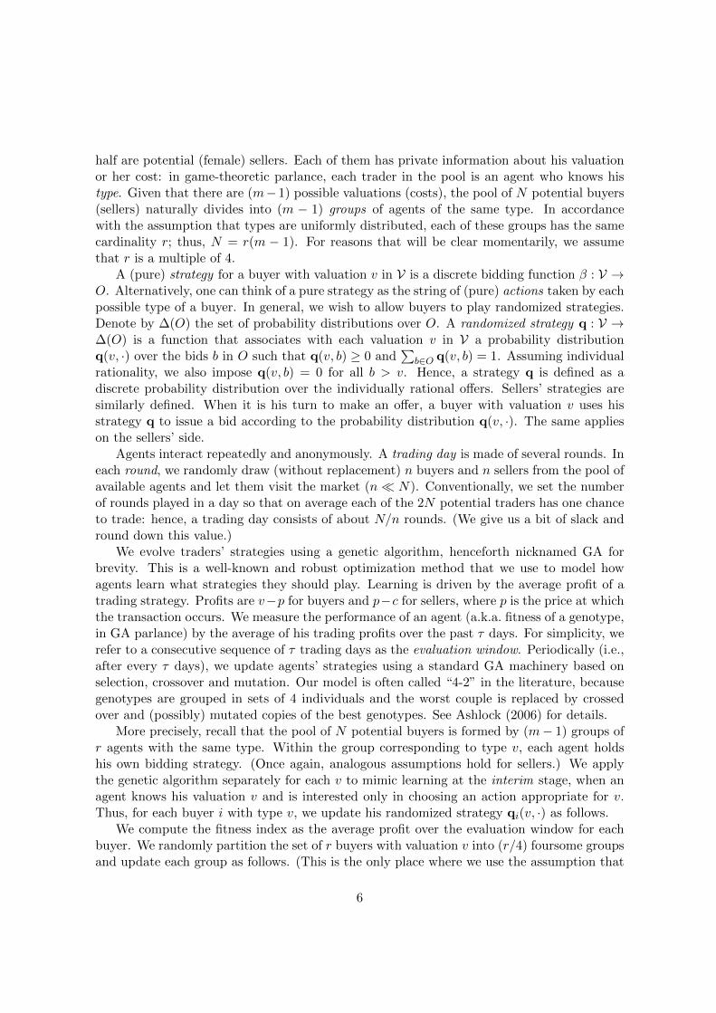
half are potential (female) sellers. Each of them has private information about his valuationor her cost: in game-theoretic parlance, each trader in the pool is an agent who knows histype. Given that there are (m−1) possible valuations (costs), the pool of N potential buyers(sellers) naturally divides into (m − 1) groups of agents of the same type. In accordancewith the assumption that types are uniformly distributed, each of these groups has the samecardinality r; thus, N = r(m − 1). For reasons that will be clear momentarily, we assumethat r is a multiple of 4.
A (pure) strategy for a buyer with valuation v in V is a discrete bidding function β : V →O. Alternatively, one can think of a pure strategy as the string of (pure) actions taken by eachpossible type of a buyer. In general, we wish to allow buyers to play randomized strategies.Denote by ∆(O) the set of probability distributions over O. A randomized strategy q : V →∆(O) is a function that associates with each valuation v in V a probability distributionq(v, ·) over the bids b in O such that q(v, b) ≥ 0 and
∑b∈O q(v, b) = 1. Assuming individual
rationality, we also impose q(v, b) = 0 for all b > v. Hence, a strategy q is defined as adiscrete probability distribution over the individually rational offers. Sellers’ strategies aresimilarly defined. When it is his turn to make an offer, a buyer with valuation v uses hisstrategy q to issue a bid according to the probability distribution q(v, ·). The same applieson the sellers’ side.
Agents interact repeatedly and anonymously. A trading day is made of several rounds. Ineach round, we randomly draw (without replacement) n buyers and n sellers from the pool ofavailable agents and let them visit the market (n� N). Conventionally, we set the numberof rounds played in a day so that on average each of the 2N potential traders has one chanceto trade: hence, a trading day consists of about N/n rounds. (We give us a bit of slack andround down this value.)
We evolve traders’ strategies using a genetic algorithm, henceforth nicknamed GA forbrevity. This is a well-known and robust optimization method that we use to model howagents learn what strategies they should play. Learning is driven by the average profit of atrading strategy. Profits are v−p for buyers and p−c for sellers, where p is the price at whichthe transaction occurs. We measure the performance of an agent (a.k.a. fitness of a genotype,in GA parlance) by the average of his trading profits over the past τ days. For simplicity, werefer to a consecutive sequence of τ trading days as the evaluation window. Periodically (i.e.,after every τ days), we update agents’ strategies using a standard GA machinery based onselection, crossover and mutation. Our model is often called “4-2” in the literature, becausegenotypes are grouped in sets of 4 individuals and the worst couple is replaced by crossedover and (possibly) mutated copies of the best genotypes. See Ashlock (2006) for details.
More precisely, recall that the pool of N potential buyers is formed by (m− 1) groups ofr agents with the same type. Within the group corresponding to type v, each agent holdshis own bidding strategy. (Once again, analogous assumptions hold for sellers.) We applythe genetic algorithm separately for each v to mimic learning at the interim stage, when anagent knows his valuation v and is interested only in choosing an action appropriate for v.Thus, for each buyer i with type v, we update his randomized strategy qi(v, ·) as follows.
We compute the fitness index as the average profit over the evaluation window for eachbuyer. We randomly partition the set of r buyers with valuation v into (r/4) foursome groupsand update each group as follows. (This is the only place where we use the assumption that
6
4 divides r exactly.) Let f1 ≥ f2 ≥ f3 ≥ f4 be the fitness indices for the four agents in agroup. (Ties are broken randomly.) The two individuals with the largest fitnesses produceby crossover two “siblings” that replace the other two individuals with the (lower) fitnessesf3 and f4. Crossover is applied using the standard one-point operator: given two randomizedactions q(v, b) and q′(v, b), we pick a random position w and generate the siblings’ actions
Mutation is applied to the siblings’ actions in two ways. First, inspired by Lettau (1997),with probability linearly decreasing in time (as measured by the cumulative number of rounds)we substitute one of the siblings’ (randomized) actions with a pure action selected withuniform probability among all bids that are individually rational with respect to v. Second,again with probability linearly decreasing in time, we apply a zero-mean additive shock to onecomponent of the other sibling’s action and accordingly renormalize his randomized strategy.
This process is repeated for each v across the corresponding groups. Hence, the actionsthat make up buyers’ strategies are separately (and simultaneously) evolved. This matchesthe intuition that learning takes place during the interim stage. The evolutionary success ofan individual is based on his capability to gain higher profits with respect to other traderswith the same valuation (or cost), while his overall gains depend on the actions that peopleare similarly evolving for different valuations and costs. Agents strive for higher profits withintheir peers but trade across the whole population.
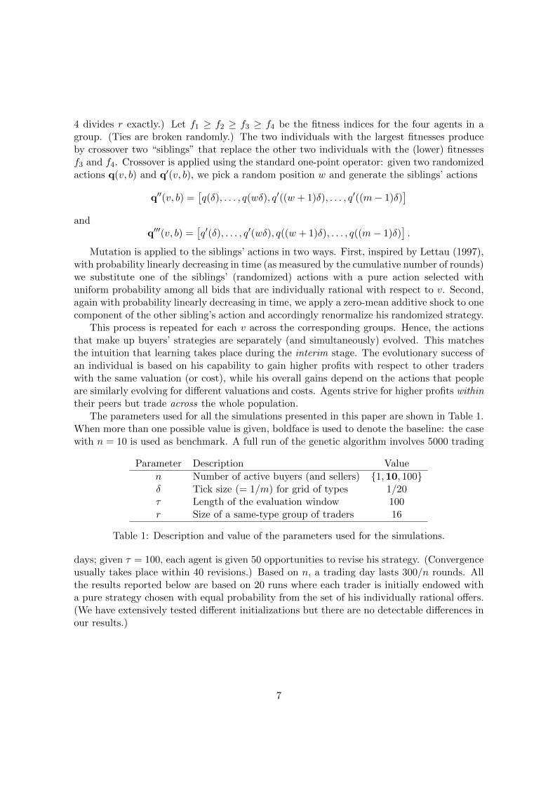
The parameters used for all the simulations presented in this paper are shown in Table 1.When more than one possible value is given, boldface is used to denote the baseline: the casewith n = 10 is used as benchmark. A full run of the genetic algorithm involves 5000 trading
Parameter Description Value
n Number of active buyers (and sellers) {1,10, 100}δ Tick size (= 1/m) for grid of types 1/20τ Length of the evaluation window 100r Size of a same-type group of traders 16
Table 1: Description and value of the parameters used for the simulations.
days; given τ = 100, each agent is given 50 opportunities to revise his strategy. (Convergenceusually takes place within 40 revisions.) Based on n, a trading day lasts 300/n rounds. Allthe results reported below are based on 20 runs where each trader is initially endowed witha pure strategy chosen with equal probability from the set of his individually rational offers.(We have extensively tested different initializations but there are no detectable differences inour results.)
7
4 Simultaneous order clearing: Results
This section presents the outcome of our simulations for the case of simultaneous order-clearing. We keep this section brief, because we find it more instructive to provide moredetails and expand the analysis of the continuous double auction.2 Therefore, we restrictattention only on our main focus: the evolution of strategic behavior when the market growsin size. Additional statistics and figures, such as the dynamics of transaction prices or traders’profit as learning progresses, have been curtailed for brevity.
Recall Theorem 1 in Section 2.2: strategic misrepresentation should shrink to zero as thenumber n of active traders on each side of the market in the market increases. Hence, asn grows, all traders should learn to be price takers. In a nutshell, we show that this is notwarranted. Even a search procedure as powerful as our genetic algorithm may fail to learn“price-taking” behavior.
For each possible valuation v, there are r = 16 buyers. (As usual, analogous statementshold for sellers.) Each of these i = 1, 2, . . . , r buyers of type v is associated with a (possiblyrandomized) strategy qi(v, ·), so our genetic algorithm maintains, compares and updatesr = 16 different strategies for a type v. At the end of a simulation, the algorithm evolvesstrategies that tend to have very similar fitness indices but need not be identical. In otherwords, buyers of the same type v are not constrained to learn the same strategy as far asthey find a way to attain similar profits.
The richness of strategic behavior that the genetic algorithm may generate can be visuallyappreciated using the following representation. For each v in the grid, we randomly pick onebuyer i of type v and generate a bid bi(v) using his strategy qi(v, ·). Then we join thesepairs of points (v, bi(v)) and obtain a bidding function that shows a realization of bids foreach of the types of a buyer. This “sampled” bidding function is noisy and should not beexpected to exhibit special mathematical properties, except for those implied by individualrationality: the graph of bidding (asking) functions is always below (above) true valuations(costs), represented by the bisector. Moving from left to right, Figure 1 displays a bundle ofthree different “sampled” bidding and asking functions for n = 1, 10, 100. The competitiveprice p∗ = 0.5 is depicted as a dashed horizontal line. Price-taking behavior is equivalent tostating an offer equal to the true valuation (cost) so it is represented by the bisector.
Looking at the picture, a few regularities emerge very clearly. Bidding and asking functiontend to be increasing in types, as it should be expected. Moreover, as we move from n = 1to n = 10, there is a clear shift towards truth-telling behavior. Increasing the number oftraders make the environment more competitive and hence introduces positive incentives forall types to learn and bid more aggressively. The more people around, the riskier it is to lie sothat all traders reduce the amount of their strategic misrepresentation. This aligns perfectlywith the result in Rustichini et al. (1994). But, when notching up from n = 10 to n = 100,this effect seems to evaporate. What is going on?
In order to answer, we remove the noise and look at the two “smoothed” trading functionsthat for each v (or c) plot the average over 20 runs of the expected bid (ask) for each group of
2 With obvious modifications, Results 1–3 listed in Section 5 for the continuous double auction hold alsofor the call market.
8
0.2 0.4 0.6 0.8
0.0
0.2
0.4
0.6
0.8
1.0
c, v
S(c
), B
(v)
0.2 0.4 0.6 0.8
0.0
0.2
0.4
0.6
0.8
1.0
c, v
S(c
), B
(v)
0.2 0.4 0.6 0.8
0.0
0.2
0.4
0.6
0.8
1.0
c, v
S(c
), B
(v)
Figure 1: Bundles of realized trading functions for n = 1, 10, 100 (from left to right).
type v (c). Moving from left to right, these are displayed in Figure 2 for n = 1, 10, 100. Whenwe go from n = 1 to n = 10, the intuition above is fully confirmed. Moving from n = 10 ton = 100, we see that it holds only for the marginal traders with valuations or costs aroundp∗ = 1/2. A moment of thought explains the puzzle. Under simultaneous-order clearing,all traders trade at a single price which (as n increases) is increasingly likely to be set bythe marginal traders. Bids and asks from extramarginal traders do not matter because theyare extremely unlikely to trade anyway; hence, there is no sufficient push for them to learnanything. Similarly, bids and asks from deeply intramarginal traders do not matter becausetrade is going to occur at price p∗ for any offer sufficiently away from p∗; again, there is nosufficient drift for learning to be price-takers. The market protocol is so robust that mereprice-taking behavior from the marginal traders is sufficient to yield the competitive price p∗.All the same, such robustness makes it highly unlikely that non-marginal traders may learnthe (unique) symmetric equilibrium.
0.2 0.4 0.6 0.8
0.0
0.2
0.4
0.6
0.8
1.0
v, c
S(c
), B
(v)
0.2 0.4 0.6 0.8
0.0
0.2
0.4
0.6
0.8
1.0
v, c
S(c
), B
(v)
0.2 0.4 0.6 0.8
0.0
0.2
0.4
0.6
0.8
1.0
v, c
S(c
), B
(v)
Figure 2: Average trading functions for n = 1, 10, 100 (from left to right).
9
4.1 Quality control for the GA strategies
We speak of the evolved trading strategies as an “equilibrium” profile that is learned byagents. However, it is clear by its nature that the genetic algorithm produces simply anapproximation and thus we need to provide some form of quality control. A natural measurefor the goodness of computational approximations to an equilibrium profile is suggested bythe notion of an ε-equilibrium.
For simplicity, we recall its definition with reference to a game with complete information.Using customary notation, assume that G = (n, S, u) is a game with n players, S = S1 ×. . . × Sn is the space of strategy profiles and u is the vector of n payoff functions for eachplayer. As usual, assume that players maximize expected payoffs. Given ε > 0, we say thata (possibly randomized) strategy profile σ is an ε-equilibrium if, for all players i and for allstrategies si in Si,
ui(σi, σ−i) ≥ ui(si, σ−i)− ε (1)
Clearly, σ is a Nash equilibrium if and only if (1) holds for ε = 0. Therefore, if we denoteby ε∗(σ) ≥ 0 the least ε that satisfies (1), we obtain a direct estimate of the “distance” thatseparates σ from being an equilibrium. Roughly speaking, ε∗(σ) is a worst-case measure forthe temptation of at least one agent to break away from the strategy profile σ. The lowerε∗(σ), the lower the push towards exploring alternative strategies. The extension of thisnotion to a game with incomplete information requires to check the analog of (1) for all typesti of each player i: ui(σi(ti), σ−i; ti) ≥ ui(si(ti), σ−i; ti)− ε.
The notion of ε-equilibrium applies to a given strategy profile σ. An evolutionary processlike our genetic algorithm, however, is unlikely to lead always to the same strategy profile.Each run of GA, in fact, ultimately evolves strategy profiles that are similar but not necessar-ily identical. Hence, we need to find a measure of quality control ε∗(GA) taking into accountthat each run of GA may end up recommending slightly different strategy profiles. To thispurpose, we extend the worst-case logic underlying the notion of ε-equilibrium as follows.Recall that we execute a batch of 20 runs of GA. At the end of each run k = 1, 2, . . . , 20, GAevolves a strategy profile σk. Assuming that all other agents play their part of σk, we checkfor all types ti of each player i the difference between his average payoff from playing whatGA recommends (that is, σk(ti)) and an arbitrary pure strategy:
20∑k=1
ui(σki (ti), σ
k−i; ti)
20≥
20∑k=1
ui(si(ti), σk−i; ti)
20− ε (2)
We define ε∗(GA) ≥ 0 as the least ε that satisfies (2). It provides a direct estimate of the“distance” that separates playing according to GA from being an optimal choice (againstany of the pure strategies). This value is used to apply a t-test for the null hypothesis thatε∗ = 0.
Table 2 collects and display the data used for our quality control. Each row in the toppanel reports the number n of traders on each side of the market, the value of ε∗(GA), thetype of the agent for whom the incentive to deviate is greatest, the offer that constitutes hisoptimal deviation and the p-value for the null hypothesis. For instance, the first row in thepanel for GA reports the information that a seller with cost c = 0.30 can make an additional
10
n ε∗ type offer p-value
1 0.0033 c = 0.30 0.45 0.25GA 10 0.0060 c = 0.25 0.30 0.0197
100 0.0014 c = 0.20 0.25 0.13
1 0.0858 v = 0.95 0.70 10−12
TT 10 0.0480 v = 0.65 0.60 0.0438100 0.0009 c = 0.10 0.40 0.27
Table 2: Quality control for the trading strategies evolved by GA in a call market.
average profit of 0.0033 by offering an ask price of 0.45 instead of complying with GA’srecommendation. This additional gain is not sufficiently high to reject the null hypothesisfor any reasonable level of confidence. It is apparent that ε∗(GA) is sufficiently close to zerofor n = 1 and n = 100. For n = 10, ε∗(GA) is still negligible although statistically significantonly at a confidence level above 2%. The left panel of Figure 3 provides a detailed graphicalrepresentation for the values of ε for the sellers’ costs. (Due to the symmetry of our model,the graph for the buyers’ valuations is analogous.) It is worth noting that the highest valuesof ε cluster around intramarginal traders of intermediate strength.
0.05 0.2 0.3 0.4 0.5 0.6 0.7 0.8 0.9 1
n =1n =10n =100
Costs
Eps
ilon
0.00
00.
001
0.00
20.
003
0.00
40.
005
0.95 0.85 0.75 0.65 0.55 0.45 0.35 0.25 0.15 0.05
n =1n =10n =100
Values
Eps
ilon
0.00
0.02
0.04
0.06
0.08
Figure 3: From left to right: values of ε∗ for sellers (GA) and buyers (TT).
For comparison, the bottom panel of Table 2 provides the same information under theassumption that the strategy profiles are generated by truth-telling (TT). Consistent withRustichini et al. (1994), the p-values for ε∗(TT) are sharply increasing in n: the hypothesisε∗(TT) = 0 for n = 1 is rejected for any reasonable level of confidence; on the other hand,this hypothesis goes unscathed for n = 100. A simpler way to summarize the evidence is tofocus on economic relevance and look at the order magnitude of ε∗: for any n under GA andfor n = 100 under TT, this is measured in thousandths; on the other hand, for n = 1, 10under TT, it is measured in hundredths. The strength of the average temptation to deviatecomes out sizeably different. The right panel of Figure 3 provides details for the values of
11
ε for the buyers’ valuations; note the different scale for the y-axis. (Sellers’ costs lead to asimilar graph.) For n = 1, there is an approximately monotonic relationship between thevalue of ε and the strength of a trader.
5 Asynchronous order clearing: Results
This section presents the outcome of our simulations for the case of asynchronous order-clearing. We first give evidence that our GA converges to a steady state that we dub the“equilibrium” outcome; see Dawid (1999) for a similar approach in an environment simplerthan ours. Next, we describe and evaluate the trading strategies evolved by our simulations.Section 6 elaborates on how these strategies compare with another class of equilibria providedin the literature.
5.1 Transaction prices and profits
We begin with a quick look at the effects of evolving trading strategies on some fundamentalparameters of the market. Our first item is the time series of transaction prices. The leftpanel in Figure 4 shows a typical sample of realized prices for the baseline sampled at days t =100, 500, 1000, 1500, 2000 and 5000. Note that the width of the vertical bands is proportional
Time series
Pric
e
0.25
0.50
0.75
100 500 1000 1500 2000 5000
0.3
0.4
0.5
0.6
0.7
Trading day
Pric
e
0 1000 2000 3000 4000 5000
Figure 4: On the left, realized transaction prices at fixed times. On the right, average (black),median (red) and interquartile range (dashed) of the transaction prices for each period.
to the number of transactions. Therefore, as learning progresses, trading prices become lessvolatile and volume increases. Moreover, the transaction prices approach the competitiveprice p∗ in the long run. The right panel exhibits the average (in black) and the median dailyprice (in red), together with the first and third quartile of the distribution of the intradaytransaction prices.
12
Result 1 In a continuous double auction under uniform priors,3 the evolution of tradingstrategies stabilizes prices around the competitive price p∗.
Furthermore, the amount of dispersion of prices around p∗ is a decreasing function of thenumber n of traders in the market as shown in Table 3. This is aligned with well-known
n µ σ
1 0.506 0.12410 0.497 0.053100 0.499 0.014
Table 3: Average price µ and standard deviation σ of the intraday price for different markets.
general convergence results for trading protocols based on the alternative assumption of si-multaneous order clearing; see Rustichini et al. (1994) for the k-double auction and Mendel-son (1985) for Walrasian trading. On the other hand, it is understood that, ceteris paribus,there is higher variability in the price of the continuous double auction as a consequence ofthe assumptions of asynchronous order clearing and random arrival of traders.
Result 2 If n1 > n2, the distribution of the transaction price P (n2) is more diffuse thanP (n1).
Similarly reassuring results hold for the aggregate profits. The left panel in Figure 5 showsthe average daily gain per trader for a typical simulation run. Traders, who initially enter themarketplace making individually rational but otherwise random offers, coevolutively learn toextract much higher profits from trade. In turn, as shown in the right panel, this leads to anincrease in the volume of transactions effected within a trading day.
We conclude that evolution leads to trading strategies that are jointly fit to maximizeoverall gains from trade. However, by construction, the GA does not attempt to maximizethese latter ones. Each agent strives to learn and improve his private gains within the groupof traders of his own type while the environment is coevolutively changing. Hence, theglobally successful extraction of the trading surplus is a byproduct of the joint and unrelatedmaximizations of individual profits.
Figure 6 separately exhibits how the average gain per type evolves over time for buyersand sellers. The left panel shows the average profit of buyers with valuations in the set{0.95, 0.9, 0.8, 0.7, 0.6, 0.5, 0.45} arranged from the strongest (v = 0.95) to the weakest (v =0.45) as we move downwards. Analogously, the right panel depicts the average profit ofsellers with costs in {0.05, 0.1, 0.2, 0.3, 0.4, 0.5, 0.55} arranged from the strongest (c = 0.05)to the weakest (c = 0.55). Profits are role-symmetric (up to the inevitable noise). Gains areincreasing in valuations and decreasing in costs: stronger traders realize higher gains fromtrade, while marginal traders (with valuations and costs close to p∗) reap minute profits.Indeed, zooming in on the bottom lines of Figure 6 shows that gains shrink over time for themarginal types. This is due to the gradual improvement of the strategies used by the strongintramarginal traders that makes them much less susceptible to being exploited by weakermarginal agents.
3 For brevity, we leave this qualification implicit in the statement of similar following results.
13
0.05
0.06
0.07
0.08
0.09
0.10
Trading day
Ave
rage
dai
ly p
rofit
0 1000 2000 3000 4000 5000
7080
9010
011
012
013
0
Trading day
Vol
ume
0 1000 2000 3000 4000 5000
Figure 5: Traders’ average profit (left) and transaction volume (right) for each period.
0.0
0.1
0.2
0.3
0.4
Buyers
Trading day
Ave
rage
dai
ly p
rofit
0 1000 2000 3000 4000 5000
0.0
0.1
0.2
0.3
0.4
Sellers
Trading day
Ave
rage
dai
ly p
rofit
0 1000 2000 3000 4000 5000
Figure 6: Average daily gains for buyers (left) and sellers (right). Groups of traders arearranged from top to bottom according to their strength.
14
Result 3 The evolution of trading strategies improves aggregate profits and is more beneficialfor stronger traders.
5.2 Trading strategies
The genetic algorithm mimics an attempt to learn equilibrium strategies. Proceeding as inSection 4, we present our results. Moving from left to right, Figure 8 displays a bundle ofthree “sampled” bidding and asking functions for n = 1, 10, 100. As before, the competitiveprice p∗ = 0.5 is represented by a dashed line. There is a sharp dependence of the shape of
0.2 0.4 0.6 0.8
0.0
0.2
0.4
0.6
0.8
1.0
c, v
S(c
), B
(v)
0.2 0.4 0.6 0.8
0.0
0.2
0.4
0.6
0.8
1.0
c, v
S(c
), B
(v)
0.2 0.4 0.6 0.80.
00.
20.
40.
60.
81.
0
c, v
S(c
), B
(v)
Figure 7: Bundles of trading functions for n = 1, 10, 100 (from left to right).
the trading strategies on the number n of agents. The pattern is even more transparent ifwe remove noise and look at the “average” trading functions, reported in Figure 8. As the
0.2 0.4 0.6 0.8
0.0
0.2
0.4
0.6
0.8
1.0
v, c
S(c
), B
(v)
0.2 0.4 0.6 0.8
0.0
0.2
0.4
0.6
0.8
1.0
c, v
S(c
), B
(v)
0.2 0.4 0.6 0.8
0.0
0.2
0.4
0.6
0.8
1.0
c, v
S(c
), B
(v)
Figure 8: Average trading functions for n = 1, 10, 100 (from left to right).
market gets thicker, all intramarginal traders become less aggressive until (as clearly visiblefor n = 100) they almost always offer exactly the competitive price p∗. On the other hand,the variability of the bidding and asking functions for extramarginal traders is quite large
15
and increasing in n: bids (asks) for v < 0.5 (c > 0.5) in Figure 7 fluctuate a lot. The simpleexplanation is that extramarginal agents trade very rarely and, consequently, get almost nochances to learn: the GA has no push to learn because it is pointlessly trying to optimize azero-profit constant function. The contrast between the rightmost panels from Figure 2 andFigure 8 is particularly striking: under simultaneous order clearing, only marginal tradersget very strong incentives to learn, while under asynchronous order clearing learning takesplace for all intramarginal traders. Moreover, these latter ones learn to be price-makers andoffer a price equal to the competitive price p∗.
Indeed, a closer look at the trading functions confirms that all intramarginal agents learnto play a pure strategy. Up to the inevitable noise inherent to the GA, each of them ends upmaking an offer equal to p∗. Figure 9 displays a typical set of genotypes (probability vectors)for the whole population when n = 100. The box on the left panel naturally divides into twotriangles. The bottom triangle pertains to buyers; the top triangle to sellers. We describeonly the buyers’ side; the analog holds for the sellers’. Probabilities are color-coded with(bright) yellow and (dark) red meaning 1 and 0, respectively. The colors along the verticalsegment between the x-axis and the bisector represent the randomized strategy of a buyerof type v over his bids. For instance, consider the vertical segment at v = 0.8: the only bidwith non-null probability (yellow) is p∗ = 0.5, while there is zero mass (red) on all the otherchoices in O.
Values / Costs
Bid
/ A
sk
0.2
0.4
0.6
0.8
1.0
0.05 0.25 0.5 0.6 0.7 0.8 0.9
Values
Max
Pro
babi
lity
0.5
0.6
0.7
0.8
0.9
1.0
0.05 0.5 0.6 0.7 0.8 0.9
Figure 9: Left panel: randomized strategies as a color-coded map with hues representingdifferent values of the probabilities. Right panel: plot of the modal value of the probabilitydistribution for each type of buyer when n = 100.
The diffusion of the red color demonstrates that positive probability is attached to asmall handful of bids and asks. For n = 100, the right panel of Figure 9 plots maxb∈O qi(v, b)for each buyer i by adjoining values around v. Whenever this probability is close to 1, thecorresponding agent is using a pure strategy. (It is understood that negligible noise is anintrinsic feature of GA.) All intramarginal traders offer the same price p∗. Extramarginal
16
traders may end up with a nontrivial randomized strategy, but the previous discussion hasexplained that this is ultimately irrelevant.
Result 4 As n increases, the trading strategies of the intramarginal agents move towardsprice-making: they learn to make a constant offer equal to the competitive price.
This is our most important result. Ceteribus paribus, the details of the order clearing rulefor the market protocols determine what kind of trading strategies we expect agents to learn.Regardless of whether order clearing is simultaneous or asynchronous, as the market growsin size, there is convergence to the competitive outcome where (almost) all trades take placeat price p∗. However, the trading strategies used by agents evolve in very different directions.Under simultaneous order clearing, marginal traders make truthful offers which set up theprice for everybody else and this deprives stronger intramarginal traders of the incentives tolearn and be price takers. Under asynchronous order clearing, all intramarginal traders endup acting as price-makers.
6 Comparative analysis
This last section compares the equilibrium strategies evolved by the genetic algorithm againstthe current benchmark in the literature, as provided by Zhan and Friedman (2007) or ZFfor short. They study the continuous double auction in an environment like ours, underthe same assumptions of Section 2.3. However, they restrict the choice of the bidding andasking functions to subsets of functions that are easily interpreted as “markdowns” on v and“markups” on c. (For simplicity, we usually speak only of markups.) They look at threepossibilities, but the leading example is the family of standard markups defined by
β(v) = v(1−md) and a(c) = c(1 +mu), (3)
where md,mu ≥ 0 are the markdown and markup coefficients.The major difference between GA and ZF is apparent. ZF search for equilibria in pure
strategies within a (restricted) parametric class and do this by running an exhaustive search;GA search for equilibria in randomized strategies within a (general) nonparametric class bya non-exhaustive evolutionary approach. A second subtler but important difference is thatZF consider ex ante equilibria, where the optimality of a strategy is evaluated assuming thatthe trader does not know his own type and hence must look at the expected payoff overall his private types. Instead, following standard game-theoretic practice, we derive interimequilibria where each agent evaluates payoffs using knowledge of his own private type (butnot others’). In other words, ZF constrains all types of a player to adopt the same markup;we allow each type of a player to pick his own markup.
Using computer simulations, ZF searches for ex ante equilibria4 within the class of stan-dard markup strategies and finds unique pairs of equilibrium coefficients: md = mu = 0.3 forn = 10, and md = 0.4,mu = 0.3 for n = 100. (We have independently confirmed this result.)ZF does not study the case n = 1; using their methodology, we obtain md = mu = 0.3 as
4 They look at two cases: cartels and single players. We consider only this latter, as it is more appropriate.
17
unique equilibrium values. (More precisely, we find that this constitutes an ε-equilibriumwith ε = 0.00002.)
ZF considers the performance of these markup equilibrium strategies with respect toallocative inefficiency and traders’ surpluses. (The allocative inefficiency is defined as thecomplement to 1 of the ratio between the realized surplus and the maximum attainablesurplus.) Table 4 compares the allocative inefficiency incurred by GA and ZF in a continuousdouble auction. It is apparent that allocative inefficiency declines as the market grows in
n 1 10 100
GA 0.196 0.084 0.048ZF 0.202 0.115 0.052
Table 4: Allocative inefficiencies for the continuous double auction.
size, regardless of whether trading strategies are obtained by GA or ZF.
Result 5 Allocative inefficiency is decreasing in market size. A plausible conjecture is thatit vanishes as n ↑ ∞.
A quick look confirms that the equilibrium strategies in ZF yield an allocative inefficiencyslightly superior than those evolved by GA, but are still within the same order of magnitude.This may suggest that ZF is in some respect a comparable approach. We are going to arguethat this impression is deceptive, because it fails to properly account for the strategic issuesthat underlie traders’ behavior. Equilibrium strategies per se do not attempt to maximizeoverall gains from trade. Allocative efficiency is only a byproduct of the individual effort tomaximize private gains. Hence, an equilibrium should be judged by its strategic plausibilityrather than by its collateral social effects.
Our claim is that ZF has two serious shortcomings from a strategic point of view. Thefirst one is that it imposes an unjustified asymmetry between buyers and sellers. Figure 10displays the average trading gains per type using GA or ZF strategies, for n = 1, 10, 100.The first panel plots average gains for buyers’ types under GA. (We omit the panel forsellers because it is virtually identical.) The second and third panel show the average gains
Figure 10: From left to right: average gains for buyers (GA), buyers (ZF) and sellers (ZF).
18
using ZF’s equilibrium strategies for buyers’ and sellers’ types, respectively. To help a directcomparison, the scale on the y-axis is the same for the three panels and traders’ types onthe x-axis are always arranged by decreasing strength. As expected, stronger traders reaphigher gains. However, it is apparent that ZF’s trading strategies let buyers extract moresurplus than sellers of equal strength, in spite of the perfect balance in the assumptions overthe trading environment.
This asymmetry in outcomes is due to a flaw in the definition of the standard markupstrategies. Define the strength of a bid b as its distance from the lowest bid (b = 0); similarly,let the strength of an ask a be its distance from the highest ask (a = 1). A profile of tradingstrategies is role-symmetric when the strengths of the bid and the ask issued by traders ofequal strength x are the same; that is, when β(x) = 1−α(1−x). Cervone et al. (2009) showsthat ZF’s markup strategies are not role-symmetric and hence lead to equilibrium outcomesthat favor buyers over sellers. To overcome this limitation, it introduces a role-symmetricformulation called convex markup and illustrates its advantages by means of a comparisonover different market protocols.
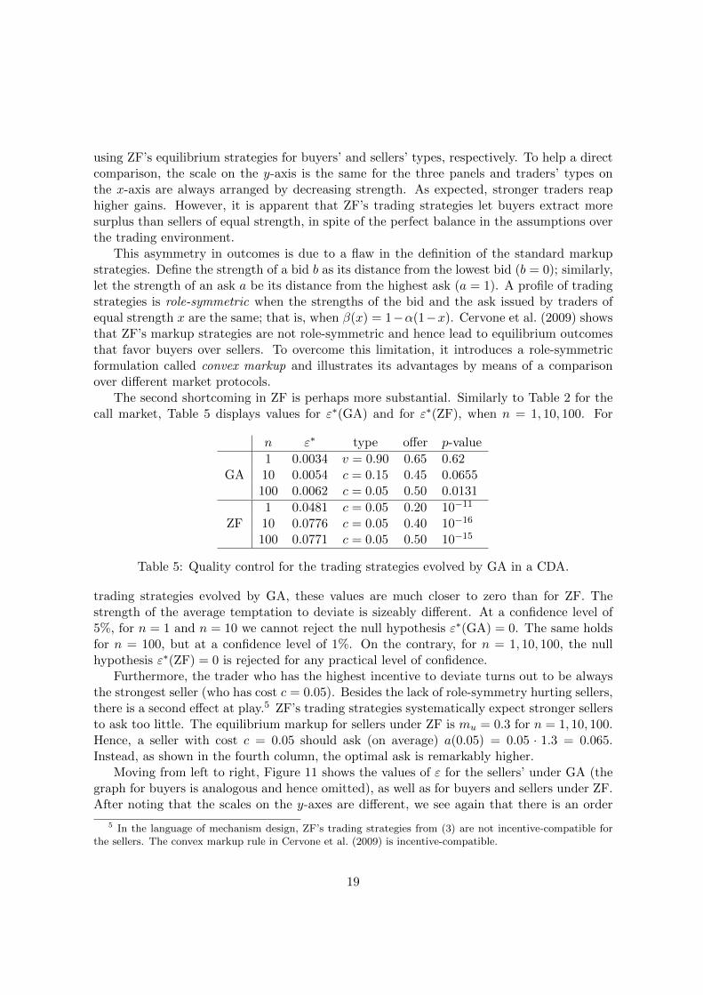
The second shortcoming in ZF is perhaps more substantial. Similarly to Table 2 for thecall market, Table 5 displays values for ε∗(GA) and for ε∗(ZF), when n = 1, 10, 100. For
n ε∗ type offer p-value
1 0.0034 v = 0.90 0.65 0.62GA 10 0.0054 c = 0.15 0.45 0.0655
100 0.0062 c = 0.05 0.50 0.0131
1 0.0481 c = 0.05 0.20 10−11
ZF 10 0.0776 c = 0.05 0.40 10−16
100 0.0771 c = 0.05 0.50 10−15
Table 5: Quality control for the trading strategies evolved by GA in a CDA.
trading strategies evolved by GA, these values are much closer to zero than for ZF. Thestrength of the average temptation to deviate is sizeably different. At a confidence level of5%, for n = 1 and n = 10 we cannot reject the null hypothesis ε∗(GA) = 0. The same holdsfor n = 100, but at a confidence level of 1%. On the contrary, for n = 1, 10, 100, the nullhypothesis ε∗(ZF) = 0 is rejected for any practical level of confidence.
Furthermore, the trader who has the highest incentive to deviate turns out to be alwaysthe strongest seller (who has cost c = 0.05). Besides the lack of role-symmetry hurting sellers,there is a second effect at play.5 ZF’s trading strategies systematically expect stronger sellersto ask too little. The equilibrium markup for sellers under ZF is mu = 0.3 for n = 1, 10, 100.Hence, a seller with cost c = 0.05 should ask (on average) a(0.05) = 0.05 · 1.3 = 0.065.Instead, as shown in the fourth column, the optimal ask is remarkably higher.
Moving from left to right, Figure 11 shows the values of ε for the sellers’ under GA (thegraph for buyers is analogous and hence omitted), as well as for buyers and sellers under ZF.After noting that the scales on the y-axes are different, we see again that there is an order
5 In the language of mechanism design, ZF’s trading strategies from (3) are not incentive-compatible forthe sellers. The convex markup rule in Cervone et al. (2009) is incentive-compatible.
19
of magnitude of difference between the ε∗ values for GA and ZF.
0.05 0.15 0.25 0.35 0.45 0.55 0.65 0.75 0.85 0.95
n =1n =10n =100
Costs
Eps
ilon
0.00
00.
001
0.00
20.
003
0.00
40.
005
0.00
6
0.95 0.85 0.75 0.65 0.55 0.45 0.35 0.25 0.15 0.05
n =1n =10n =100
Values
Eps
ilon
0.00
0.01
0.02
0.03
0.04
0.05
0.06
0.05 0.15 0.25 0.35 0.45 0.55 0.65 0.75 0.85 0.95
n =1n =10n =100
Costs
Eps
ilon
0.00
0.02
0.04
0.06
Figure 11: From left to right: values of ε∗ for sellers (GA), buyers (ZF) and sellers (ZF).
6.1 Evolutionary stability
This last subsection rounds up our comparison between GA and ZF using the notion of evo-lutionarily stable strategies (ESS) introduced in Maynard Smith and Price (1973). Roughlyspeaking, a profile of trading functions is an ESS if, once it is adopted, it is not susceptibleto invasion by a new strategy. This notion formalizes the “robustness” of a strategy profileas the ability to prevent the spread of competing alternatives under evolutionary pressure.We claim that ZF does not pass the test of evolutionary stability against GA.
We consider a population of agents using ZF’s trading strategies and inject a small fractionof traders playing the strategies evolved by GA. We measure the average profits made byagents using the two competing strategies. For n = 1, 10, 100, Figure 12 depicts the levelcurves for the joint distribution of average daily gains obtained by traders in the invading GApopulation versus those collected by the ZF agents. (The fraction of invading GA traders isset equal to 1/16 and we collect realized profits over 1000 trading days.)
As n increases, it is apparent that the advantage enjoyed by GA traders gets stronger.Hence, the prospect of invadability for ZF increases when the market grows in size. Theintuitive explanation is clear. The ZF equilibrium trading strategies are linear functions. Asshown in Figure 7, for n = 1 the GA strategies can be decently approximated by a linearfunction. Therefore, the scope for differentiation between ZF and GA is limited. On theother hand, as n increases, the GA strategies morph towards a flat price-making offer (forthe intramarginal traders) that is sharply different from ZF’s prescription.
The evolutionary pressure can be quantified by looking at the (average) incremental profitper trading day reaped by the invading GA agents pitted against ZF traders. For n = 100,we find a value of 0.010 as sum of an average incremental profit of −0.005 for buyers and0.025 for sellers. A “naive” statistician using a t-test for the overall value would require onlyabout 30 trading days to reject the null hypothesis that the GA strategy is less profitablethan ZF at a level of confidence of 0.1%. (Rejection would be even faster by testing only forthe sellers’ side.) Similarly, for n = 10, the evolutionary advantage to GA is 0.009 (buyers:
20
Daily average gain GA
Dai
ly a
vera
ge g
ain
ZF
50
100
150
200
250
0.00 0.05 0.10 0.15
0.00
0.05
0.10
0.15
●
Daily average gain GA
Dai
ly a
vera
ge g
ain
ZF
50
100
150 200
250
0.00 0.05 0.10 0.15
0.00
0.05
0.10
0.15
●
Daily average gain GA
Dai
ly a
vera
ge g
ain
ZF
50
100
150
200
250
300
0.00 0.05 0.10 0.15
0.00
0.05
0.10
0.15
●
Figure 12: Joint distribution of the average daily gains for GA agents (x-axis) invading a ZFpopulation (y-axis) for n = 1, 10, 100 (from left to right). The mean of the distribution isplotted as a thick point, along with the line of equal average profits.
−0.002; sellers: 0.020); a statistically significant rejection at the same level of confidencewould occur after about 550 days. For n = 1, the average incremental profit for GA is 0.002(buyers: −0.003; sellers: 0.007); more than 1000 trading days would be necessary for ananalogous statistical rejection.
Additional intuition is gained by considering Figure 13 that for n = 100 separately showsthe average incremental profits of buyers (on the left) as a function of their valuations andof sellers (on the right) as a function of their costs. (As before, the fraction of invading GA
0.2 0.4 0.6 0.8
−0.
04−
0.02
0.00
0.02
0.04
0.06
Values
Ave
rage
add
ition
al g
ain
0.2 0.4 0.6 0.8
−0.
04−
0.02
0.00
0.02
0.04
0.06
Costs
Ave
rage
add
ition
al g
ain
Figure 13: Average incremental profits for GA invading ZF: buyers (left) and sellers (right).
traders is 1/16 and we compare profits realized over 1000 trading days.) Marginal and verystrong buyers perform slightly higher under GA, while intramarginal buyers of intermediatestrength are much better off sticking with ZF. On the other hand, almost all intramarginal
21
sellers find GA more profitable than ZF and thus the stronger evolutionary pressure to breakfree from ZF and shift towards GA lies on the sellers’ side.
A The bilateral trading model
The bilateral trading model (with simultaneous order clearing) was introduced in Chatterjee andSamuelson (1983) and studied in Myerson and Satterthwaite (1983), spawning a long and still flour-ishing literature. It describes a situation where one buyer and one seller are engaged in the tradeof a single object. The environment is the same as in Section 2.1, but there are only one buyer andone seller so n = 1. Viewed as a game with incomplete information, it is equivalent to the k-doubleauction described in Section 2.2 for k = 1/2 and n = 1.
An equilibrium profile (β, α) of bidding and asking functions for the bilateral trading modelrequires that a buyer with valuation v offers a bid b = β(v) that solves
maxb
∫ 1
0
[v − α(c) + b
2
]1{b ≥ α(c)} dG(c) (4)
and a seller with cost c submits an ask a = α(c) that solves
maxa
∫ 1
0
[a+ β(v)
2− c]
1{a ≤ β(v)} dF (v), (5)
where 1{·} is the indicator function.The formal description of the bilateral trading model under asynchronous order clearing requires
only the following changes. There are two equally likely queues: the buyer arrives first, or the sellerarrives first. If a buyer with valuation v arrives first, he finds no outstanding ask and hence recordshis bid b = β(v) on the buying book and, if trade occurs, the price is b. Similarly, if a seller withcost c arrives first, she writes her ask a = α(c) on the selling book and, if trade occurs, the priceis a. Therefore, if trade occurs, it takes place at price b with probability 1/2 and at price a withprobability 1/2. Recall that, under simultaneous order clearing, the transaction price is p = (a+ b)/2.Therefore, roughly speaking, the expected value of the trading price is the same under simultaneousor asynchronous order clearing but the latter one adds some variability around it. (Formally speaking,the distribution of the trading price is a mean-preserving spread.)
Given that traders are risk neutral, this immediately translates in the strategic equivalence ofthe equilibria for the two models. We prove this claim by showing that the expected payoffs underany strategy profile (β, α) are the same for the two models. In the bilateral trading model underasynchronous order clearing, a buyer with valuation v who offers a bid b = β(v) obtains a payoff
maxb
1
2
∫ 1
0
[v − α(c)
]1{b ≥ α(c)} dG(c) +
1
2
∫ 1
0
[v − b
]1{b ≥ α(c)} dG(c). (6)
In the bilateral trading model under simultaneous order clearing, the payoff to a buyer with valuationv who offers a bid b = β(v) is given in Equation (4). Clearly, (4) and (6) are identical. A similarargument applies for the seller. Therefore, the set of equilibria under arbitrary priors for the twomodels is the same. More generally, a similar argument applies to show the strategic equivalence ofthe equilibria for a k-double auction and a continuous double auction where the buyer arrives beforethe seller with probability k. Note that, while strategic equivalence holds, equilibrium payoffs coincideonly in expectation.
22
References
[1] M. Anufriev, J. Arifovic and V. Panchenko (2010), “Efficiency of continuous double auc-tions under individual evolutionary learning with full or limited information”, CeNDEFWorking paper 10-01, University of Amsterdam.
[2] D. Ashlock (2006), Evolutionary Computation for Modeling and Optimization, Springer.
[3] R. Aumann, “Game theory”, in: J. Eatwell, M. Milgate, and P. Newman (eds.), TheNew Palgrave: A Dictionary of Economics, volume 2, Macmillan, 1987, 460–482.
[4] R. Cervone, S. Galavotti, and M. LiCalzi, “Symmetric equilibria in double auctions withmarkdown buyers and markup sellers”, in: C. Hernandez, M. Posada and A. Lopez-Paredes (eds.), Artificial Economics, Springer, 2009, 81–92.
[5] K. Chatterjee and W. Samuelson (1983), “Bargaining under incomplete information”,Operations Research 31, 835–851.
[6] H. Dawid (1999), “On the convergence of genetic learning in a double auction market”,Journal of Economic Dynamics and Control 23, 1545–1567.
[7] D. Friedman (1993), “The double auction institution: A survey”, in: D. Friedman andJ. Rust (eds.), The Double Auction Market: Institutions, Theories and Evidence, Cam-bridge (MA): Perseus Publishing, 3–25.
[8] D.K. Gode and S. Sunder (1993), “Allocative efficiency of markets with zero intelligencetraders: Market as a partial substitute for individual rationality”, Journal of PoliticalEconomy 101, 119–137.
[9] W. Leininger, P.B. Linhart, and R. Radner (1989), “Equilibria of the sealed-bid mech-anism for bargaining with incomplete information”, Journal of Economic Theory 48,63-106.
[10] M. Lettau (1997), “Explaining the facts with adaptive agents: The case of mutual fundflows”, Journal of Economic Dynamics and Control 21, 1117–1147.
[11] J.K. MacKie and M.P. Wellman (2006), “Automated markets and trading agents”, in:L. Tesfatsion and K.L. Judd (eds.), Handbook of Computational Economics, vol. 2, El-sevier, 1381–1431.
[12] J. Maynard Smith and G.R. Price (1973), “The logic of animal conflict”, Nature 246,15–18.
[13] H. Mendelson (1985), “Random competitive exchange: Price distributions and gainsfrom trade”, Journal of Economic Theory 37, 254-280.
[14] R.B. Myerson and M.A. Satterthwaite (1983), “Efficient mechanisms for bilateral trad-ing”, Journal of Economic Theory 29, 265–281.
23
[15] S. Phelps, S. Parsons, and P. McBurney (2006), “An evolutionary game-theoretic com-parison of two double-auction market designs”, in: P. Faratin and J.A. Rodriguez-Aguılar(eds.), Agent-Mediated Electronic Commerce VI, Springer, 101–114.
[16] A. Rustichini, M.A. Satterthwaite, and S.R. Williams (1994), “Convergence to efficiencyin a simple market with incomplete information”, Econometrica 62, 1041-1063.
[17] M.A. Satterthwaite and S.R. Williams (1993), “The bayesian theory of the k-doubleauction”, in: D. Friedman and J. Rust (eds.), The Double Auction Market: Institutions,Theories and Evidence, Cambridge (MA): Perseus Publishing, 99–123.
[18] M.A. Satterthwaite and S.R. Williams (2002), “The optimality of a simple market mech-anism”, Econometrica 70, 1841-1863.
[19] W. Zhan and D. Friedman (2007), “Markups in double auction markets”, Journal ofEconomic Dynamics and Control 31, 2984–3005.