59
Convergence of Stochastic Processes and Collapsing of Manifolds Xue-Mei Li The University of Warwick 6 ICSAA 12 September 2012 Bedlewo, Poland 1 / 59
Convergence of Stochastic Processes and
Collapsing of Manifolds
Xue-Mei LiThe University of Warwick
6 ICSAA12 September 2012
Bedlewo, Poland
1 / 59
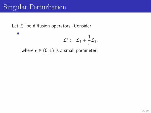
Singular Perturbation
Let Li be diffusion operators. Consider
Lε := L1 +1
εL2,
where ε ∈ (0, 1) is a small parameter.
Expand the solution, to the equation below, in ε,
∂uεt∂t
= (L1 +1
εL2)(uεt ).
uεt = u0t + εu1
t + ε2u2t + . . . .
We seek an equation for u0t , and possibly for u1
t ...
2 / 59

Singular Perturbation
Let Li be diffusion operators. Consider
Lε := L1 +1
εL2,
where ε ∈ (0, 1) is a small parameter.
Expand the solution, to the equation below, in ε,
∂uεt∂t
= (L1 +1
εL2)(uεt ).
uεt = u0t + εu1
t + ε2u2t + . . . .
We seek an equation for u0t , and possibly for u1
t ...
3 / 59
History
Orbits of celestial bodies are governed by a Hamiltoniansystem on the cotangent bundle : ut = XH(ut).On R2d , the equation is qt = ∂H
∂p, pt = −∂H
∂q.
Reduction in complexity:Suppose that the true dynamical system differs from thisHamiltonian system by order ε. After a long time of order1ε, how does the orbit deviate from that given by the
Hamiltonian system, ? V.I. Arnold, ...
4 / 59
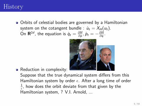
History
Orbits of celestial bodies are governed by a Hamiltoniansystem on the cotangent bundle : ut = XH(ut).On R2d , the equation is qt = ∂H
∂p, pt = −∂H
∂q.
Reduction in complexity:Suppose that the true dynamical system differs from thisHamiltonian system by order ε. After a long time of order1ε, how does the orbit deviate from that given by the
Hamiltonian system, ? V.I. Arnold, ...
5 / 59
History: Averaging and Homogeneisation
Averaging and homogenisation of parabolic PDEs trace backto: R. Khasminskii (1963), M. Freidlin (1964),
Papanicolaou-Varadhan (1973),Papanicolaou-Stroock-Varadhan (1977).
Book by A. Bensoussan,J.-L. Lions, G. Papanicolaou. 700 pages, expect to findeverything!
6 / 59
Development
In elasticity theory, e.g. A. Desimon, S. Muller, R.V. Kohn;For discrete systems, e.g. A. Gloria and F. Otto.
J.-M. Bismut “Hypoelliptic Laplacian and orbitalintegrals”, “Loops Spaces and hypoelliptic Laplacian” andcohomologies. Look for unspoken Brownian motions.
Hamilton-Jacobi equations, transportequations : E. Kosygina-F. Rezakhanlou-S.R.S. Varadhan-P.-L.Lions-P.E. Souganidis; A. Bensoussan-J. L. Lions- G.Papanicolaou.Multi scale analysis: A.J. Majda, W. E., E. Vanden-Eijnden, A.Stuart, M. Hairer, J. Mattingly and G. Pavliotis.
7 / 59
Example
Let L2 =∑d
i ,j=1 a2i ,j(x , y) ∂2
∂yi∂yj,L1 =
∑di ,j=1 a1
i ,j(x , y) ∂2
∂xi∂xj,
∂
∂t(u0
t + εu1t + ε2u2
t + . . . ) = (L1 +1
εL2)(u0
t + εu1t + ε2u2
t + . . . ).
0 = L2u0t ,
∂u0t
∂t= L1u0
t + L2u1t .
Assume that Lx2 is elliptic in variable y with the unique
invariant measure µx(dy). Then u0 is a constant in y .We integrate the second equation:
∂
∂tu0t (x) =
∫ (∑a1i ,j(x , y)
∂2
∂xi∂xjµx(dy)
)u0t (x) +
∫L2u1
t µx(dy)
=
∫ (∑a1i ,j(x , y)µx(dy)
) ∂2
∂xi∂xju0t (x)
= L1u0t (x).
8 / 59
Example
Let L2 =∑d
i ,j=1 a2i ,j(x , y) ∂2
∂yi∂yj,L1 =
∑di ,j=1 a1
i ,j(x , y) ∂2
∂xi∂xj,
∂
∂t(u0
t + εu1t + ε2u2
t + . . . ) = (L1 +1
εL2)(u0
t + εu1t + ε2u2
t + . . . ).
0 = L2u0t ,
∂u0t
∂t= L1u0
t + L2u1t .
Assume that Lx2 is elliptic in variable y with the unique
invariant measure µx(dy). Then u0 is a constant in y .We integrate the second equation:
∂
∂tu0t (x) =
∫ (∑a1i ,j(x , y)
∂2
∂xi∂xjµx(dy)
)u0t (x) +
∫L2u1
t µx(dy)
=
∫ (∑a1i ,j(x , y)µx(dy)
) ∂2
∂xi∂xju0t (x)
= L1u0t (x).
9 / 59
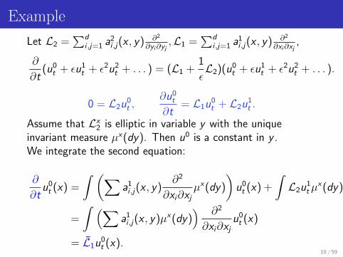
Example
Let L2 =∑d
i ,j=1 a2i ,j(x , y) ∂2
∂yi∂yj,L1 =
∑di ,j=1 a1
i ,j(x , y) ∂2
∂xi∂xj,
∂
∂t(u0
t + εu1t + ε2u2
t + . . . ) = (L1 +1
εL2)(u0
t + εu1t + ε2u2
t + . . . ).
0 = L2u0t ,
∂u0t
∂t= L1u0
t + L2u1t .
Assume that Lx2 is elliptic in variable y with the unique
invariant measure µx(dy). Then u0 is a constant in y .We integrate the second equation:
∂
∂tu0t (x) =
∫ (∑a1i ,j(x , y)
∂2
∂xi∂xjµx(dy)
)u0t (x) +
∫L2u1
t µx(dy)
=
∫ (∑a1i ,j(x , y)µx(dy)
) ∂2
∂xi∂xju0t (x)
= L1u0t (x).
10 / 59
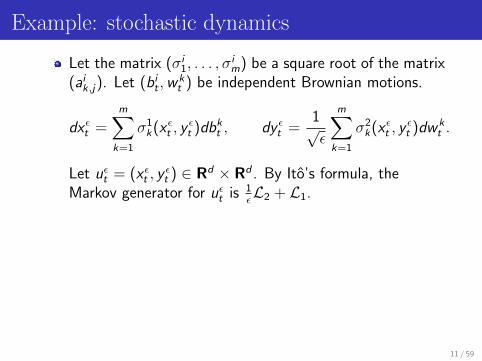
Example: stochastic dynamics
Let the matrix (σi1, . . . , σ
im) be a square root of the matrix
(aik,j). Let (bi
t ,wkt ) be independent Brownian motions.
dx εt =m∑
k=1
σ1k(x εt , y
εt )dbk
t , dy εt =1√ε
m∑k=1
σ2k(x εt , y
εt )dw k
t .
Let uεt = (x εt , yεt ) ∈ Rd × Rd . By Ito’s formula, the
Markov generator for uεt is 1εL2 + L1.
The special feature of uεt is that it consists of twocomponents, living in the product space Rd × Rd , oneof which is clearly the fast variable.
In general there will be more interactions, intertwinningssuch as rotations. We may consider uεt lives in a spaceupstairs; x εt or y εt the projection. The total space, whereuεt lives, is locally a product space.
11 / 59
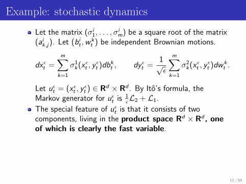
Example: stochastic dynamics
Let the matrix (σi1, . . . , σ
im) be a square root of the matrix
(aik,j). Let (bi
t ,wkt ) be independent Brownian motions.
dx εt =m∑
k=1
σ1k(x εt , y
εt )dbk
t , dy εt =1√ε
m∑k=1
σ2k(x εt , y
εt )dw k
t .
Let uεt = (x εt , yεt ) ∈ Rd × Rd . By Ito’s formula, the
Markov generator for uεt is 1εL2 + L1.
The special feature of uεt is that it consists of twocomponents, living in the product space Rd × Rd , oneof which is clearly the fast variable.
In general there will be more interactions, intertwinningssuch as rotations. We may consider uεt lives in a spaceupstairs; x εt or y εt the projection. The total space, whereuεt lives, is locally a product space.
12 / 59
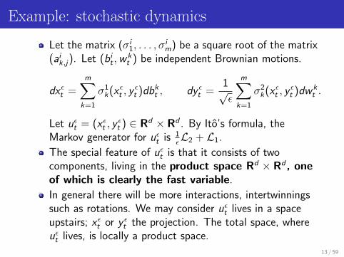
Example: stochastic dynamics
Let the matrix (σi1, . . . , σ
im) be a square root of the matrix
(aik,j). Let (bi
t ,wkt ) be independent Brownian motions.
dx εt =m∑
k=1
σ1k(x εt , y
εt )dbk
t , dy εt =1√ε
m∑k=1
σ2k(x εt , y
εt )dw k
t .
Let uεt = (x εt , yεt ) ∈ Rd × Rd . By Ito’s formula, the
Markov generator for uεt is 1εL2 + L1.
The special feature of uεt is that it consists of twocomponents, living in the product space Rd × Rd , oneof which is clearly the fast variable.
In general there will be more interactions, intertwinningssuch as rotations. We may consider uεt lives in a spaceupstairs; x εt or y εt the projection. The total space, whereuεt lives, is locally a product space.
13 / 59
Examples
We note three classes of spaces, where singular perturbationproblem occurs naturally.
1 Symplectic manifolds, e.g. with a completely integrablefamily of Hamiltonian. [L. 08]
2 The frame bundles of a Riemannian manifold M [L.12].Why is it interesting? ut = Hut (e0), u0(e0) = v0 gives the
geodesic flow.3 The Hopf fibration: π : S3 → S2, with Berger’s metrics.
This is expected to extend to manifolds with contactstructures.
Something in common: there is an almost symplectic structurefor (2) and a contact structure for (3), J. Gray 59.
14 / 59
Examples
We note three classes of spaces, where singular perturbationproblem occurs naturally.
1 Symplectic manifolds, e.g. with a completely integrablefamily of Hamiltonian. [L. 08]
2 The frame bundles of a Riemannian manifold M [L.12].Why is it interesting? ut = Hut (e0), u0(e0) = v0 gives the
geodesic flow.3 The Hopf fibration: π : S3 → S2, with Berger’s metrics.
This is expected to extend to manifolds with contactstructures.
Something in common: there is an almost symplectic structurefor (2) and a contact structure for (3), J. Gray 59. 15 / 59
The Hopf Fibration
Let SU(2) =
{(z w−w z
) ∣∣∣ z ,w ∈ C, |z |2 + |w |2 = 1
}.
1 There is a right action by U(1) on SU(2), defined below:
[z ,w ]e iθ
=⇒ [e iθz , e iθw ] =
(e iθ 00 e−iθ
)(z w−w z
).
2 Denote by M = SU(2)/U(1), the space of of orbits.Define: π to be the projection to the orbit.
3 The action by U(1) is smooth, effective and proper.
π−1(Ui )diffeo
Ui × S1
Ui ⊂ M
πProj
There is, hence, a unique manifoldstructure on M s.t. π is smooth, surjective, a submersion(Tp is surjective), and a fibration with fibre S1.
16 / 59
The Hopf Fibration
Let SU(2) =
{(z w−w z
) ∣∣∣ z ,w ∈ C, |z |2 + |w |2 = 1
}.
1 There is a right action by U(1) on SU(2), defined below:
[z ,w ]e iθ
=⇒ [e iθz , e iθw ] =
(e iθ 00 e−iθ
)(z w−w z
).
2 Denote by M = SU(2)/U(1), the space of of orbits.Define: π to be the projection to the orbit.
3 The action by U(1) is smooth, effective and proper.
π−1(Ui )diffeo
Ui × S1
Ui ⊂ M
πProj
There is, hence, a unique manifoldstructure on M s.t. π is smooth, surjective, a submersion(Tp is surjective), and a fibration with fibre S1.
17 / 59
The Hopf Fibration
Let SU(2) =
{(z w−w z
) ∣∣∣ z ,w ∈ C, |z |2 + |w |2 = 1
}.
1 There is a right action by U(1) on SU(2), defined below:
[z ,w ]e iθ
=⇒ [e iθz , e iθw ] =
(e iθ 00 e−iθ
)(z w−w z
).
2 Denote by M = SU(2)/U(1), the space of of orbits.Define: π to be the projection to the orbit.
3 The action by U(1) is smooth, effective and proper.
π−1(Ui )diffeo
Ui × S1
Ui ⊂ M
πProj
There is, hence, a unique manifoldstructure on M s.t. π is smooth, surjective, a submersion(Tp is surjective), and a fibration with fibre S1.
18 / 59

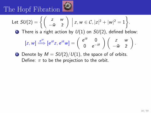
The Hopf Fibration
Let SU(2) =
{(z w−w z
) ∣∣∣ z ,w ∈ C, |z |2 + |w |2 = 1
}.
1 There is a right action by U(1) on SU(2), defined below:
[z ,w ]e iθ
=⇒ [e iθz , e iθw ] =
(e iθ 00 e−iθ
)(z w−w z
).
2 Denote by M = SU(2)/U(1), the space of of orbits.Define: π to be the projection to the orbit.
3 The action by U(1) is smooth, effective and proper.
π−1(Ui )diffeo
Ui × S1
Ui ⊂ M
πProj
There is, hence, a unique manifoldstructure on M s.t. π is smooth, surjective, a submersion(Tp is surjective), and a fibration with fibre S1.
19 / 59
The Hopf Fibration
Let SU(2) =
{(z w−w z
) ∣∣∣ z ,w ∈ C, |z |2 + |w |2 = 1
}.
1 There is a right action by U(1) on SU(2), defined below:
[z ,w ]e iθ
=⇒ [e iθz , e iθw ] =
(e iθ 00 e−iθ
)(z w−w z
).
2 Denote by M = SU(2)/U(1), the space of of orbits.Define: π to be the projection to the orbit.
3 The action by U(1) is smooth, effective and proper.
π−1(Ui )diffeo
Ui × S1
Ui ⊂ M
πProj
There is, hence, a unique manifoldstructure on M s.t. π is smooth, surjective, a submersion(Tp is surjective), and a fibration with fibre S1.
20 / 59
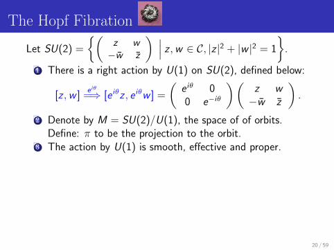
The Hopf Fibration
Let SU(2) =
{(z w−w z
) ∣∣∣ z ,w ∈ C, |z |2 + |w |2 = 1
}.
1 There is a right action by U(1) on SU(2), defined below:
[z ,w ]e iθ
=⇒ [e iθz , e iθw ] =
(e iθ 00 e−iθ
)(z w−w z
).
2 Denote by M = SU(2)/U(1), the space of of orbits.Define: π to be the projection to the orbit.
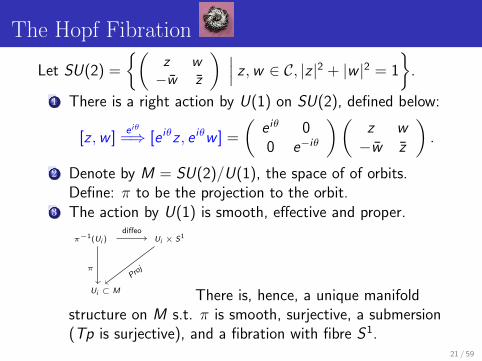
3 The action by U(1) is smooth, effective and proper.
π−1(Ui )diffeo
Ui × S1
Ui ⊂ M
πProj
There is, hence, a unique manifoldstructure on M s.t. π is smooth, surjective, a submersion(Tp is surjective), and a fibration with fibre S1.
21 / 59
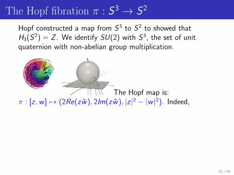
The Hopf fibration π : S3 → S2
Hopf constructed a map from S3 to S2 to showed thatH3(S2) = Z . We identify SU(2) with S3, the set of unitquaternion with non-abelian group multiplication.
The Hopf map is:π : [z ,w ] 7→ (2Re(zw), 2Im(zw), |z |2 − |w |2). Indeed,
1 SU(2)/U(1) ∼ CP1, the complex projective space. Itconsists of equivalent classes in C2, [z ,w ] ∼ [λz , λw ],λ 6= 0.
2 CP1 ∼ S2. Let φ : R2 → S2 − { North Pole} be thestereographic projection. Take [z : w ] ∈ CP1 with w 6= 0,
define [z : w ]→ zw∈ C ∼ R2 φ→ S2.
22 / 59
The Hopf fibration π : S3 → S2
Hopf constructed a map from S3 to S2 to showed thatH3(S2) = Z . We identify SU(2) with S3, the set of unitquaternion with non-abelian group multiplication.
The Hopf map is:π : [z ,w ] 7→ (2Re(zw), 2Im(zw), |z |2 − |w |2). Indeed,
1 SU(2)/U(1) ∼ CP1, the complex projective space. Itconsists of equivalent classes in C2, [z ,w ] ∼ [λz , λw ],λ 6= 0.
2 CP1 ∼ S2. Let φ : R2 → S2 − { North Pole} be thestereographic projection. Take [z : w ] ∈ CP1 with w 6= 0,
define [z : w ]→ zw∈ C ∼ R2 φ→ S2.
23 / 59
The Hopf fibration π : S3 → S2
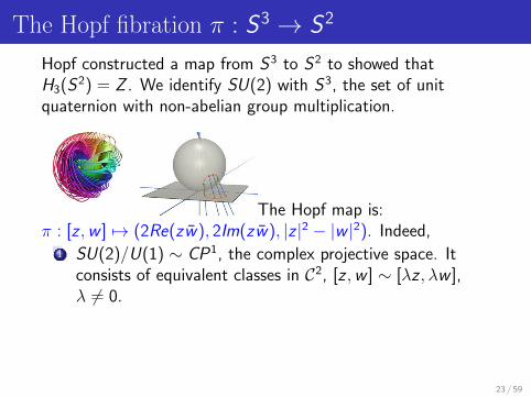
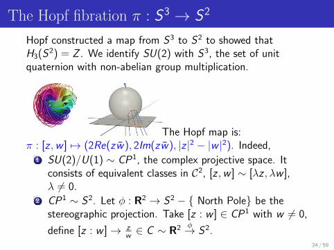
Hopf constructed a map from S3 to S2 to showed thatH3(S2) = Z . We identify SU(2) with S3, the set of unitquaternion with non-abelian group multiplication.
The Hopf map is:π : [z ,w ] 7→ (2Re(zw), 2Im(zw), |z |2 − |w |2). Indeed,
1 SU(2)/U(1) ∼ CP1, the complex projective space. Itconsists of equivalent classes in C2, [z ,w ] ∼ [λz , λw ],λ 6= 0.
2 CP1 ∼ S2. Let φ : R2 → S2 − { North Pole} be thestereographic projection. Take [z : w ] ∈ CP1 with w 6= 0,
define [z : w ]→ zw∈ C ∼ R2 φ→ S2.
24 / 59
The projection Tπ : TS3 → TS2
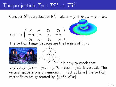
Consider S3 as a subset of R4. Take z = y1 + iy2,w = y3 + iy4.
Tyπ = 2
y3 y4, y1 y2
−y4 y3 y2, −y1
y1, y2, −y3, −y4
.
The vertical tangent spaces are the kernels of Tuπ.
It is easy to check thatV (y1, y2, y3, y4) = −y2∂1 + y1∂2 − y4∂3 + y3∂4 is vertical. Thevertical space is one dimensional. In fact at [z ,w ] the verticalvector fields are generated by d
dt[e itz , e itw ].
25 / 59
The Riemannian Structures, π : S3 → S2
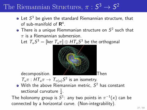
Let S3 be given the standard Riemannian structure, thatof sub-manifold of R4.There is a unique Riemmanian structure on S2 such thatπ is a Riemannian submersion.Let TuS3 = [ker Tuπ]⊕ HTuS3 be the orthogonal
decomposition. ThenTuπ : HTuπ → Tπ(u)S
2 is an isometry.With the above Riemannian metric, S2 has constantsectional curvature 1
4.
The holonomy group is S1: any two points in π−1(x) can beconnected by a horizontal curve. (Non-integrability).
26 / 59
The Riemannian Structures, π : S3 → S2
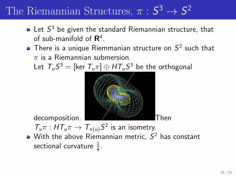
Let S3 be given the standard Riemannian structure, thatof sub-manifold of R4.There is a unique Riemmanian structure on S2 such thatπ is a Riemannian submersion.Let TuS3 = [ker Tuπ]⊕ HTuS3 be the orthogonal
decomposition. ThenTuπ : HTuπ → Tπ(u)S
2 is an isometry.With the above Riemannian metric, S2 has constantsectional curvature 1
4.
The holonomy group is S1: any two points in π−1(x) can beconnected by a horizontal curve. (Non-integrability).
27 / 59
The Pauli matrices
SU(2) is a simply connected Lie group. Its Lie algebra
su(2) consists of matrices of the form,
(ia β−β −ia
)where a ∈ R, β ∈ C. Define〈A,B〉 = 1
2trace(AB∗).
The pauli matrices form an o.n.b.:
X1 =
(i 00 −i
),X2 =
(0 −11 0
),X3 =
(0 ii 0
).
The structural constants are {−2,−2,−2}, see J. Milnor[Mil76] for a discussion on classifications of threedimensional Lie groups.Let Xi denote also the corresponding left invariant vectorfields.[X2,X3] = −2X1, [X3,X1] = −2X2, [X1,X2] = −2X3. Thehorizontal distributions are not integrable.
28 / 59

The Pauli matrices
SU(2) is a simply connected Lie group. Its Lie algebra
su(2) consists of matrices of the form,
(ia β−β −ia
)where a ∈ R, β ∈ C. Define〈A,B〉 = 1
2trace(AB∗).
The pauli matrices form an o.n.b.:
X1 =
(i 00 −i
),X2 =
(0 −11 0
),X3 =
(0 ii 0
).
The structural constants are {−2,−2,−2}, see J. Milnor[Mil76] for a discussion on classifications of threedimensional Lie groups.
Let Xi denote also the corresponding left invariant vectorfields.[X2,X3] = −2X1, [X3,X1] = −2X2, [X1,X2] = −2X3. Thehorizontal distributions are not integrable.
29 / 59
The Pauli matrices
SU(2) is a simply connected Lie group. Its Lie algebra
su(2) consists of matrices of the form,
(ia β−β −ia
)where a ∈ R, β ∈ C. Define〈A,B〉 = 1
2trace(AB∗).
The pauli matrices form an o.n.b.:
X1 =
(i 00 −i
),X2 =
(0 −11 0
),X3 =
(0 ii 0
).
The structural constants are {−2,−2,−2}, see J. Milnor[Mil76] for a discussion on classifications of threedimensional Lie groups.Let Xi denote also the corresponding left invariant vectorfields.[X2,X3] = −2X1, [X3,X1] = −2X2, [X1,X2] = −2X3. Thehorizontal distributions are not integrable. 30 / 59

Berger’s Spheres
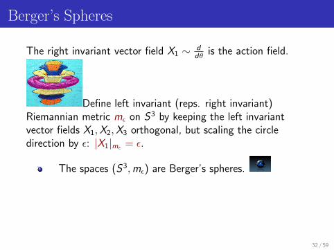
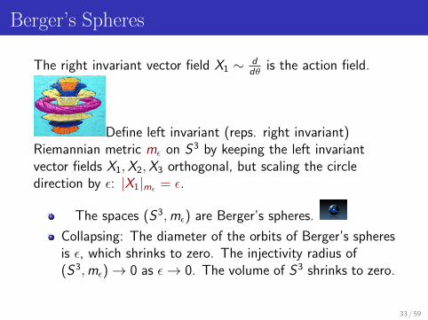
The right invariant vector field X1 ∼ ddθ
is the action field.
Define left invariant (reps. right invariant)Riemannian metric mε on S3 by keeping the left invariantvector fields X1,X2,X3 orthogonal, but scaling the circledirection by ε: |X1|mε = ε.
The spaces (S3,mε) are Berger’s spheres.
Collapsing: The diameter of the orbits of Berger’s spheresis ε, which shrinks to zero. The injectivity radius of(S3,mε)→ 0 as ε→ 0. The volume of S3 shrinks to zero.
31 / 59
Berger’s Spheres
The right invariant vector field X1 ∼ ddθ
is the action field.
Define left invariant (reps. right invariant)Riemannian metric mε on S3 by keeping the left invariantvector fields X1,X2,X3 orthogonal, but scaling the circledirection by ε: |X1|mε = ε.
The spaces (S3,mε) are Berger’s spheres.
Collapsing: The diameter of the orbits of Berger’s spheresis ε, which shrinks to zero. The injectivity radius of(S3,mε)→ 0 as ε→ 0. The volume of S3 shrinks to zero.
32 / 59
Berger’s Spheres
The right invariant vector field X1 ∼ ddθ
is the action field.
Define left invariant (reps. right invariant)Riemannian metric mε on S3 by keeping the left invariantvector fields X1,X2,X3 orthogonal, but scaling the circledirection by ε: |X1|mε = ε.
The spaces (S3,mε) are Berger’s spheres.
Collapsing: The diameter of the orbits of Berger’s spheresis ε, which shrinks to zero. The injectivity radius of(S3,mε)→ 0 as ε→ 0. The volume of S3 shrinks to zero.
33 / 59
Collapsing of (S3,mε)
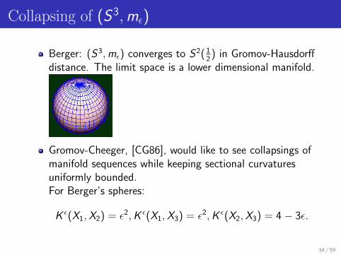
Berger: (S3,mε) converges to S2( 12) in Gromov-Hausdorff
distance. The limit space is a lower dimensional manifold.
Gromov-Cheeger, [CG86], would like to see collapsings ofmanifold sequences while keeping sectional curvaturesuniformly bounded.For Berger’s spheres:
K ε(X1,X2) = ε2,K ε(X1,X3) = ε2,K ε(X2,X3) = 4− 3ε.
34 / 59
Why bounded sectional curvature?
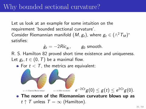
Let us look at an example for some intuition on therequirement ‘bounded sectional curvature’.Consider Riemannian manifold (M , gt), where gt ∈ (∧2TM)∗
satisfies:gt = −2Ricgt , g0 smooth.
R. S. Hamilton 82 proved short time existence and uniqueness.Let gt , t ∈ (0,T ) be a maximal flow.
For t < T , the metrics are equivalent:
e−2Ctg(0) ≤ g(t) ≤ e2Ctg(0).The norm of the Riemannian curvature blows up ast ↑ T unless T =∞ (Hamilton).
35 / 59
Gromov-Hausdorff Convergence
A sequence (Mn, gn) converges strongly to (M , g) if there arediffeomorphisms φn : Mn → M such that (φn)∗gn → g .
Let A,B be sets in a metric space (X , d), define
dH(A,B) = inf{ε > 0 : B ⊂ Aε,A ⊂ Bε}.
For any point x in A there is a point y in B s.t.d(x , y) ≤ ε.
Gromov-Hausdorff distance between metric spaces:
dGH((X1, d1), (X2, d2)) = inf(φi :(Xi ,di )→(X ,d))
{dH(φ1(X1), φ2(X2))}.
Here φi are isometric embeddings.
Two metric spaces are isometric if their distance equals zero.The set of equivalent classes of compact metric spaces withdiameter bounded above is compact.
36 / 59
Measured G-H convergence
If (Mn, gn)→ (M , g) how about the spectral of the Laplacian?
K. Fukaya introduced Measured Gromov-Hausdorffconvergence: consider the metric spaces (Mn, gn, µn)where µn is a probability measure.limn→∞(Mn, gn) = (M , g) in measured Gromov-Hausdorffdistance if there is a family of measurable maps:ψn : Mn → M and positive numbers εn → 0 such that|d(ψn(p), ψn(q))− d(p, q)| < εn, (ψn(Mn))εn = M and(ψn)∗(µn)→ µ weakly.
One a Riemannian manifold of finite volume, we take themeasure to be the volume measure normalised to 1.
Berger’s sphere converges in measured Gromov-Hausdorffdistance.
37 / 59
Fukaya’s theorem on spectral convergence
Theorem (Fukaya [Fuk87])
Let DM(n,D) be the closure of the class of Riemannianmanifolds whose sectional curvature K is bounded between −1and 1 in the measured Gromov-Hausdorff distance. Let λk(M)be the kth-eigenvalue of a manifold M ∈ DM(n,D).Then λk can be extended to a continuous function onDM(n,D)− {(point, 1)}. For each element(X , µ) ∈ DM(n,D), λk(X ) is the kth eigenvalue of aselfadjoint operator on L2(X , µ).
Y. Ogura [Ogu01], Y. Ogura-S. Taniguchi [OT96] studied theconvergence of Brownian motions, in a suitable sense, a familyof Riemannian manifolds (Mn, gn) that converges inKasue-Kumura’s spectral distance, where the distancebetween heat kernels at time t (weighted by e−(t+1/t)) areinvolved.
38 / 59
Fukaya’s theorem on spectral convergence
Theorem (Fukaya [Fuk87])
Let DM(n,D) be the closure of the class of Riemannianmanifolds whose sectional curvature K is bounded between −1and 1 in the measured Gromov-Hausdorff distance. Let λk(M)be the kth-eigenvalue of a manifold M ∈ DM(n,D).Then λk can be extended to a continuous function onDM(n,D)− {(point, 1)}. For each element(X , µ) ∈ DM(n,D), λk(X ) is the kth eigenvalue of aselfadjoint operator on L2(X , µ).
Y. Ogura [Ogu01], Y. Ogura-S. Taniguchi [OT96] studied theconvergence of Brownian motions, in a suitable sense, a familyof Riemannian manifolds (Mn, gn) that converges inKasue-Kumura’s spectral distance, where the distancebetween heat kernels at time t (weighted by e−(t+1/t)) areinvolved. 39 / 59
The Spectrum on (S3,mε)
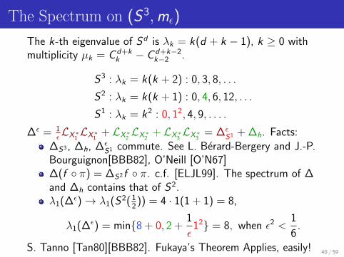
The k-th eigenvalue of Sd is λk = k(d + k − 1), k ≥ 0 withmultiplicity µk = C d+k
k − C d+k−2k−2 .
S3 : λk = k(k + 2) : 0, 3, 8, . . .
S2 : λk = k(k + 1) : 0, 4, 6, 12, . . .
S1 : λk = k2 : 0, 12, 4, 9, . . . .
∆ε = 1εLX∗
1LX∗
1+ LX∗
2LX∗
2+ LX∗
3LX∗
3= ∆ε
S1 + ∆h. Facts:∆S3 , ∆h, ∆ε
S1 commute. See L. Berard-Bergery and J.-P.Bourguignon[BBB82], O’Neill [O’N67]∆(f ◦ π) = ∆S2f ◦ π. c.f. [ELJL99]. The spectrum of ∆and ∆h contains that of S2.λ1(∆ε)→ λ1(S2( 1
2)) = 4 · 1(1 + 1) = 8,
λ1(∆ε) = min{8 + 0, 2 +1
ε12} = 8, when ε2 <
1
6.
S. Tanno [Tan80][BBB82]. Fukaya’s Theorem Applies, easily! 40 / 59
Convergences associated to collapsing of the
manifolds
41 / 59
Horizontal Lifts
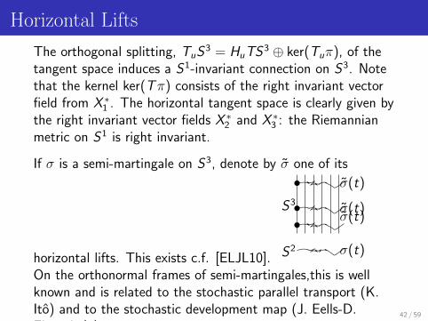
The orthogonal splitting, TuS3 = HuTS3 ⊕ ker(Tuπ), of thetangent space induces a S1-invariant connection on S3. Notethat the kernel ker(Tπ) consists of the right invariant vectorfield from X ∗1 . The horizontal tangent space is clearly given bythe right invariant vector fields X ∗2 and X ∗3 : the Riemannianmetric on S1 is right invariant.
If σ is a semi-martingale on S3, denote by σ one of its
horizontal lifts. This exists c.f. [ELJL10].
•
••
σ(t)S2
S3
σ(t)
σ(t)σ(t)
On the orthonormal frames of semi-martingales,this is wellknown and is related to the stochastic parallel transport (K.Ito) and to the stochastic development map (J. Eells-D.Elworthy) ).
42 / 59
Invariant vector fields on S3
As a Lie group there are three left invariant X Li and right
invariant vector fields XRi . Since the metric on the sphere with
round metric is bi-invariant, they form an o.n.b at each point.The right invariant vector fields are horizontal, andπ∗(XR
2 ), π∗(X 33 ) is orthonormal at π(u). However the
projection do not induce vector fields on S2. This can also beeasily deduced from the fact that on S2 there is no nowherevanishing vector fields.The left invariant vector fields do projects to vector fields onS2. By the same reason the projection cannot be generate twoeverywhere independent vector fields. Hence the left invariantvector fields cannot lie in the horizontal distribution, and theleft invariant vector field X L
1 is not in the kernel of Tπ.
43 / 59
Sub-Riemannian Geometry on S3
The horizontal distribution has the following properties:Any point can be reached from a given one by a horizontalcurve (Hormander condition).The horizontal lift of a geodesic on S3, or on (S3,mε) givenbelow, is a horizontal geodesic (of minimal length among allhorizontal curves).
44 / 59
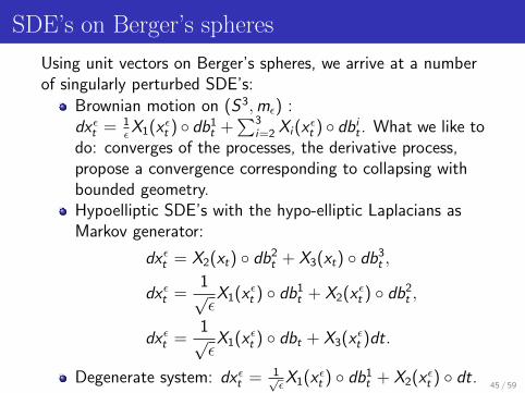
SDE’s on Berger’s spheres
Using unit vectors on Berger’s spheres, we arrive at a numberof singularly perturbed SDE’s:
Brownian motion on (S3,mε) :dx εt = 1
εX1(x εt ) ◦ db1
t +∑3
i=2 Xi(x εt ) ◦ dbit . What we like to
do: converges of the processes, the derivative process,propose a convergence corresponding to collapsing withbounded geometry.Hypoelliptic SDE’s with the hypo-elliptic Laplacians asMarkov generator:
dx εt = X2(xt) ◦ db2t + X3(xt) ◦ db3
t ,
dx εt =1√ε
X1(x εt ) ◦ db1t + X2(x εt ) ◦ db2
t ,
dx εt =1√ε
X1(x εt ) ◦ dbt + X3(x εt )dt.
Degenerate system: dx εt = 1√εX1(x εt ) ◦ db1
t + X2(x εt ) ◦ dt.45 / 59
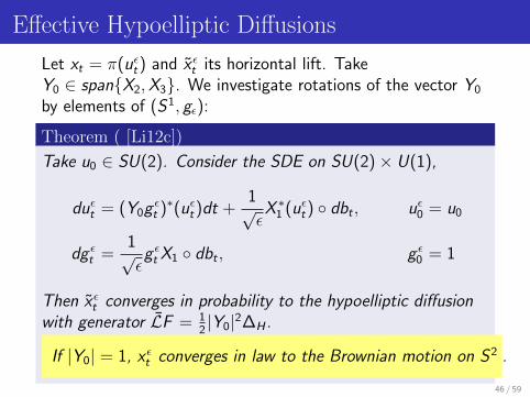
Effective Hypoelliptic Diffusions
Let xt = π(uεt ) and x εt its horizontal lift. TakeY0 ∈ span{X2,X3}. We investigate rotations of the vector Y0
by elements of (S1, gε):
Theorem ( [Li12c])
Take u0 ∈ SU(2). Consider the SDE on SU(2)× U(1),
duεt = (Y0g εt )∗(uεt )dt +1√ε
X ∗1 (uεt ) ◦ dbt , uε0 = u0
dg εt =1√ε
g εt X1 ◦ dbt , g ε0 = 1
Then x εt converges in probability to the hypoelliptic diffusionwith generator LF = 1
2|Y0|2∆H .
If |Y0| = 1, x εt converges in law to the Brownian motion on S2 .
46 / 59
Remark
We have mentioned that a Brownian motion on S2 cannot beconstructed by an SDE on R2driven than less than 3independent Brownian motion, e.g.
dxt =m∑i=1
Vi(xt) ◦ dbit
with m < 3.In the above we constructed a Brownian motion on S2 withone driving Brownian motion. We remark that : (1) The SDEon S3 does not project to an SDE on S2.(2) With one single driving Brownian motion, we obtain ahypoelliptic Brownian motion.
47 / 59
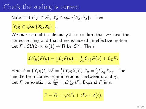
Check the scaling is correct
Note that if g ∈ S1, Y0 ∈ span{X2,X3}. Then
Y0g ∈ span{X2,X3} .
We make a multi scale analysis to confirm that we have thecorrect scaling and that there is indeed an effective motion.Let F : SU(2)× U(1)→ R be C∞. Then
Lε(g)F (u) = 1εL0F (u) + 1√
εLZg
1F (u) + LZF .
Here Z = (Y0g)∗, Z g1 = 1
2(Y0gX1)∗, L0 = 1
2LX∗
1LX∗
1. The
middle term comes from interaction between u and g .Let F be solution to ∂F
∂t= Lε(g)F . Expand F in ε,
F = F0 +√εF1 + εF2 + o(ε).
48 / 59
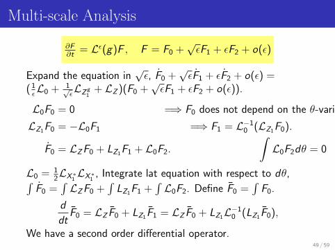
Multi-scale Analysis
∂F∂t
= Lε(g)F , F = F0 +√εF1 + εF2 + o(ε)
Expand the equation in√ε, F0 +
√εF1 + εF2 + o(ε) =
( 1εL0 + 1√
εLZg
1+ LZ )(F0 +
√εF1 + εF2 + o(ε)).
L0F0 = 0 =⇒ F0 does not depend on the θ-variable
LZ1F0 = −L0F1 =⇒ F1 = L−10 (LZ1F0).
F0 = LZF0 + LZ1F1 + L0F2.
∫L0F2dθ = 0
.
L0 = 12LX∗
1LX∗
1, Integrate lat equation with respect to dθ,∫
F0 =∫LZF0 +
∫LZ1F1 +
∫L0F2. Define F0 =
∫F0.
d
dtF0 = LZ F0 + LZ1F1 = LZ F0 + LZ1L−1
0 (LZ1F0),
We have a second order differential operator.49 / 59
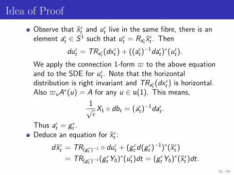
Idea of Proof
Observe that x εt and uεt live in the same fibre, there is anelement aεt ∈ S1 such that uεt = Raεt x εt . Then
duεt = TRaεt (dx εt ) + ((aεt)−1daεt)
∗(uεt ).
We apply the connection 1-form $ to the above equationand to the SDE for uεt . Note that the horizontaldistribution is right invariant and TRaεt (dx εt ) is horizontal.Also $uA∗(u) = A for any u ∈ u(1). This means,
1√ε
X1 ◦ dbt = (aεt)−1daεt .
Thus aεt = g εt .Deduce an equation for x εt :
dx εt = TR(gεt )−1 ◦ duεt + (g εt d(g εt )−1)∗(x εt )
= TR(gεt )−1(g εt Y0)∗(uεt )dt = (g εt Y0)∗(x εt )dt.
50 / 59

Proof
ddt
x εt = (g εt Y0)∗(x εt ). This bounded variation term willleads to a diffusion term in the limit.We prove the tightness of relevant measures for the weakconvergence.Let F : S3 → R be any smooth function. SinceY0 ∈ span{X2,X3},
F (x εt ) = F (u0) +3∑
j=2
∫ t
0
dF (x εs Xj)〈Xj , gεs Y0〉ds.
Note the right hand side is bounded variation term.However we seek an approximate ‘semi-martingale’decomposition, of the form, ‘martingale +drift+o(ε)-terms. To the drift term we may apply the ergodictheorem.Solve a Poisson Equation and use Stroock-Varadhan’smartingale method to identify the limits.Bensoussan-Lions-Papanicolaou [BLP76]
51 / 59
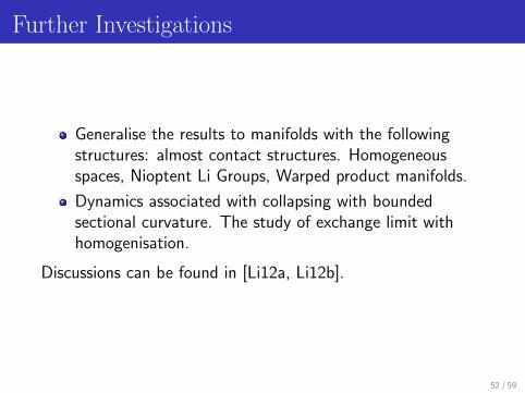
Further Investigations
Generalise the results to manifolds with the followingstructures: almost contact structures. Homogeneousspaces, Nioptent Li Groups, Warped product manifolds.
Dynamics associated with collapsing with boundedsectional curvature. The study of exchange limit withhomogenisation.
Discussions can be found in [Li12a, Li12b].
52 / 59
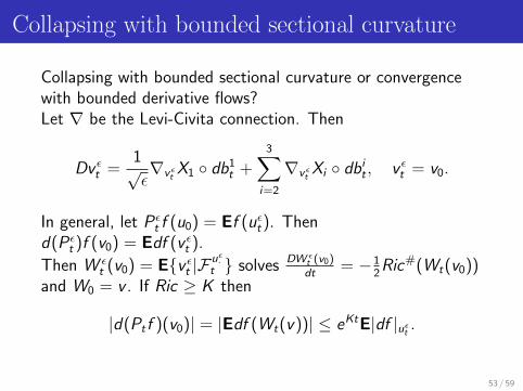
Collapsing with bounded sectional curvature
Collapsing with bounded sectional curvature or convergencewith bounded derivative flows?Let ∇ be the Levi-Civita connection. Then
Dv εt =1√ε∇vε
tX1 ◦ db1
t +3∑
i=2
∇vεtXi ◦ dbi
t , v εt = v0.
In general, let Pεt f (u0) = Ef (uεt ). Then
d(Pεt )f (v0) = Edf (v εt ).
Then W εt (v0) = E{v εt |F
uε·t } solves DW ε
t (v0)dt
= −12Ric#(Wt(v0))
and W0 = v . If Ric ≥ K then
|d(Ptf )(v0)| = |Edf (Wt(v))| ≤ eKtE|df |uεt .
53 / 59
Convergence with bounded derivatives
Since Ric bounded from below is equivalent to|∇Ptf |2 ≤ e2Kt |∇f |2, we propose to study collapsing ofmanifolds with one of the following constraints: (1)|∇Pε
t f |2ε ≤ e2Kt |∇f |2ε or (2) the derivative flows|E{v εt |F εt }|ε ≤ C |v0|ε.
54 / 59
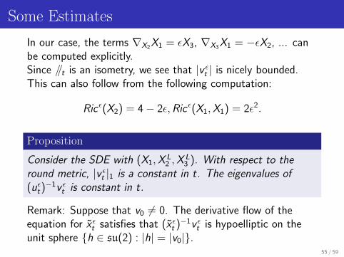
Some Estimates
In our case, the terms ∇X2X1 = εX3, ∇X3X1 = −εX2, ... canbe computed explicitly.Since //t is an isometry, we see that |v εt | is nicely bounded.This can also follow from the following computation:
Ricε(X2) = 4− 2ε,Ricε(X1,X1) = 2ε2.
Proposition
Consider the SDE with (X1,XL2 ,X
L3 ). With respect to the
round metric, |v εt |1 is a constant in t. The eigenvalues of(uεt )−1v εt is constant in t.
Remark: Suppose that v0 6= 0. The derivative flow of theequation for x εt satisfies that (x εt )−1v εt is hypoelliptic on theunit sphere {h ∈ su(2) : |h| = |v0|}.
55 / 59
Selected Refrences
Lionel Berard-Bergery and Jean-Pierre Bourguignon.Laplacians and Riemannian submersions with totallygeodesic fibres.Illinois J. Math., 26(2):181–200, 1982.
A. Bensoussan, J.L. Lions, and G. Papanicolaou.Homogeneisation, correcteurs et problemes non-lineaires.C. R. Acad. Sci. Paris Ser. A-B, 282(22):1277–A1282,1976.
Jeff Cheeger and Mikhael Gromov.Collapsing Riemannian manifolds while keeping theircurvature bounded. I.J. Differential Geom., 23(3):309–346, 1986.
K. D. Elworthy, Y. Le Jan, and Xue-Mei Li.On the geometry of diffusion operators and stochasticflows, volume 1720 of Lecture Notes in Mathematics.
56 / 59

Springer-Verlag, Berlin, 1999.
K. David Elworthy, Yves Le Jan, and Xue-Mei Li.The geometry of filtering.Frontiers in Mathematics. Birkhauser Verlag, Basel, 2010.
Kenji Fukaya.Collapsing Riemannian manifolds to ones of lowerdimensions.J. Differential Geom., 25(1):139–156, 1987.
Xue-Mei Li.Collapsing Brownian motions on the Hopf fibration.In Preparation, 2012.
Xue-Mei Li.Effective derivative flows and commutation of linearisationand averaging.Preprint, 2012.
57 / 59
Xue-Mei Li.Effective diffusions with intertwined structures.Preprint, 2012.
John Milnor.Curvatures of left invariant metrics on Lie groups.Advances in Math., 21(3):293–329, 1976.
Yukio Ogura.Weak convergence of laws of stochastic processes onRiemannian manifolds.Probab. Theory Related Fields, 119(4):529–557, 2001.
Barrett O’Neill.Submersions and geodesics.Duke Math. J., 34:363–373, 1967.
Yukio Ogura and Setsuo Taniguchi.A probabilistic scheme for collapse of metrics.
58 / 59
J. Math. Kyoto Univ., 36(1):73–92, 1996.
Shukichi Tanno.A characterization of the canonical spheres by thespectrum.Math. Z., 175(3):267–274, 1980.
59 / 59


