University of Pennsylvania University of Pennsylvania ScholarlyCommons ScholarlyCommons Technical Reports (CIS) Department of Computer & Information Science April 1992 Convergence of Stochastic Processes Convergence of Stochastic Processes Robert Mandelbaum University of Pennsylvania Follow this and additional works at: https://repository.upenn.edu/cis_reports Recommended Citation Recommended Citation Robert Mandelbaum, "Convergence of Stochastic Processes", . April 1992. University of Pennsylvania Department of Computer and Information Science Technical Report No. MS-CIS-92-30. This paper is posted at ScholarlyCommons. https://repository.upenn.edu/cis_reports/470 For more information, please contact [email protected].
Transcript
University of Pennsylvania University of Pennsylvania
ScholarlyCommons ScholarlyCommons
Technical Reports (CIS) Department of Computer & Information Science
April 1992
Convergence of Stochastic Processes Convergence of Stochastic Processes
Robert Mandelbaum University of Pennsylvania
Follow this and additional works at: https://repository.upenn.edu/cis_reports
Recommended Citation Recommended Citation Robert Mandelbaum, "Convergence of Stochastic Processes", . April 1992.
University of Pennsylvania Department of Computer and Information Science Technical Report No. MS-CIS-92-30.
This paper is posted at ScholarlyCommons. https://repository.upenn.edu/cis_reports/470 For more information, please contact [email protected].
Convergence of Stochastic Processes Convergence of Stochastic Processes
Abstract Abstract Often the best way to adumbrate a dark and dense assemblage of material is to describe the background in contrast to which the edges of the nebulosity may be clearly discerned. Hence, perhaps the most appropriate way to introduce this paper is to describe what it is not. It is not a comprehensive study of stochastic processes, nor an in-depth treatment of convergence. In fact, on the surface, the material covered in this paper is nothing more than a compendium of seemingly loosely-connected and barely-miscible theorems, methods and conclusions from the three main papers surveyed ([VC71], [Pol89] and [DL91]).
Comments Comments University of Pennsylvania Department of Computer and Information Science Technical Report No. MS-CIS-92-30.
This technical report is available at ScholarlyCommons: https://repository.upenn.edu/cis_reports/470
Following the example of [Po1891 and [Pol84], linear function notation is used whenever it can cause 110 ambiguity. Hence, instead of J g ( x ) Q ( d x ) or J g dQ for the integral with respect to a measure Q, we write Q ( g ) or simply Qg.
The Cartesia.n product symbol is @. Maximum and minimum are represented by V and A respectively. The integral symbol J appearing without limits refers to inte- gration over the entire space. The inner product of two vectors x and q5 is denoted (x, 4). Random va.riables are denoted X, Y and 2. CDF, PDF and PMF stand for Cumulative Distributive Function, Probability Density Function and Probability Mass Function respectively. The notation Z N P indicates that random variable Z has distribution P, while E p ( Z ) denotes the espectation of Z accordiilg to the distribution P. In keeping with the notation used in [?I , expectation of Z with re- spect to the underlying proba.bility measure will a,lso be denoted by P Z, as against P { a E A) which denotes the measure of set A.
N ( m , a 2 ) usua.11~ symbolises the Norma.1 distribution of mean m and variance a 2 . Boldface type is reserved for sets and vectors. Calligraphic symbols are generally used as follows: A a,nd L? refer to classes of sets; D, S and X refer to classes of functions; F, P and & refer to a classes of distributions; L1 and L2 are defined as in Section 2.6, while P ( A ) refers to the power set of a set A. ?R represents the set of real nuilll~ers, while ?R+ denotes the tlonnegative reals.
g = O ( f ) signifies that function g grows no faster than f . Similarly, g = O ( f ) signifies that g is order f , while g = o ( f ) indicates that g has asymptotic growth strictly smaller than f . Finally, g = O p ( f ) , g = O p ( f ) and g = op( . f ) indicate that the respective growth rates of g and f converge in probability to their prescribed asymptotic relationship.
All other symbols a,re defined on site.
For science, G-d is sirnpl-y the stream of tendency by which all things seek to fulfil the law of their being.
LITERATURE AND DOGMA William Arnold
1 Introduction
Often the best way to adumbrate a dark and dense assemblage of material is to describe the background in contrast to which the edges of the nebulosity may be clearly discerned. Hence, perhaps the most appropriate way to introduce this paper is to describe what it is ?tot. It is lzot a comprehensive study of stochastic processes, nor an in-depth treatment of convergence. In fact, on the surface, the material covered in this paper is nothing more than a compendium of seemingly loosely-connected and barely-miscible theorems, methods a.nd conclusions from the three main papers surveyed ([VC7 11, [PolSS] and [DLgl]).
And yet, closer inspection revea.1~ a common thread running steadily through the papers and delica.tely weaving them into a coherent and tightly-knit tapestry. It is the ambition of this paper both to describe the content and significance of each of the papers individually as well as to expose this elegant intertwining and interdependence.
The classical Bernoulli theorem states that in a sequence of n independent trials, the relative frequency of an event A converges (in probability) to the proba,bility of that event as 12 + ca [VCTl]. The need often arises to ensure that this convergence is uniform over an entire c1a.s~ of events A. In other words, representing the relative frequency of a set A E A after n trials by up) and the probability of A by PA, we require tha.t for arbitra.rily small E ,
For instance, for a distribution function P over the real line %, and a class A = {(-oo, t] : t E X), the strong law of large numbers guarantees that the proportion
of points in an interval ( -w , t ] converges almost surely to P ( t ) , while the classical Glivenko-Cantelli theorem strengthens the result by adding uniformity of convergence over all t [Po184]. However, it turns out that even in the simplest of examples, this type of uniform convergence does not necessarily hold. The first of the three papers to be discussed here, [VC71], supplies criteria on the basis of which one may judge whether a given combination of distribution P and class A boasts such uniform convergence (see Section 3). In particular, the paper demonstrates that for an arbitrary P, any so-called Vapnik-Chervonenkis (VC) class of sets will exhibit uniform convergence.
While the main thread of the second paper, [Po189], is claimed by the author to be merely a glimpse into the theory of empirical processes, one may also view the material there as a direct extension of the ideas presented in [VC71] and the generalization of the concept of uniform convergence to classes of fti~zctions. Instea,cl of the relative frequency of a set A E A a,fter n trials, u p ) , we now speak of the expectation of a function g E 6 with respect to the empirical measure P, (which puts mass 72-I at each of the sample points - see Section 4); instead of the probability of A, PA, we now speak of the expectation of g with respect to the underlying distribution P. The uniformity result we are now after is that for arbitrarily small 6 ,
This extension is more closely entwined with the ideas in [VC71] than may at first be apparent. Indeed, if one considers the class of indicator functions 6 = { I A : A E A} corresponding to the class of sets A, then, besides a rescaling factor of n'j2, the two uniformity goals (1) and (2) a,re seen to be identical: Since the empirical measure Pn puts mass 12-I a t each of the sa.mple points, Pn IA is easily identifiable as the relative frequency u?), wllile in a simila,r fashion, P la = P ( A ) .
Moreover, just as [VC71] shows t11a.t a VC class of sets will satisfy requirement ( I ) , [Pol891 shows that god (2) is a,chieved for what Pollard terms manageable classes of functions. But the plesus does not end there: It turns out that if a class of functions 6 = {Y : '9 -+ R} with bounded envelope G is such t11a.t {subgraph(g) : g E G) is a VC class of subsets of Q R, then 6 is, in fa.ct, a m.anageable class of functions [Pol89]. See Section 4 for the definition of subgraph(g) as well for an expos6 of the intricate relationship between VC classes of subsets and manageable classes of functions.
Any discourse on asymptotics must go hand in hand with a discussion of the rates at which convergence takes place. Indeed, concepts of 'rates of convergence' form the
very seam binding the delicate filigree of the asymptotic with the rather coarser and more ragged burlap of the finite.
The third paper surveyed, [DLSl], considers a bound on the rate of convergence of an estimate T,(Xn) (where Xn is the vector of n i.i.d. F sample points) to the value of a functional T ( F ) of an unknown distribution F E 3 uniformly over a class of distributions 3 . The bound involves the modulus of continuity b ( c ) [DL911 of the functional T over 3, and is shown to be attainable, to within constants, whenever T is linear and .F is convex. See Section 5 for a general discussion of [DL911 as well as Subsection 5.5 where the implications of the caveat "to within constants'' are a.na.lyzed from the perspective of Estimation Theory.
Once again, close scrutiny revea.1~ a fine enmeshment of the ideas of [DL911 with those of [VC71] and [PolSS] which a cursory consideration may dispute. Indeed, given a class of functions G, we ca,n consider each function g E G as a random variable with respect to the probability space ( 8 , 13, P), where B denotes the Bore1 field on the real line ?J? and P is some probability measure of finite va,riance. Let F be the class of margina.1 distributions of the resultant stochastic process, and choose the (linear) functional T ( F ) , F E F to be the expected value of F, i.e. T ( F ) = P g where F E F is the distribution of the random variable g E G. Convexifying F yields a form to which the results of Donoho&Liu a.re applicable, so that a bound on the rate of convergence to T ( F ) of any estima,te TT,(Xn), including the empirical expectation Pn g, uniformly over F ma,y be deduced via the modulus of continuity b(c ) . This is the a.pproach taken in Section 6 where bhe methods of [DL911 are implemented to establish bounds on ra.tes of uniform convergence for a VC class of subsets.
Of course, t,he results of [DL911 extend far beyond these rather constrained and con- trived cases to incorpora,te any convex cla,ss of distributions F and any linear func- tional T (not just the expected value with respect to the probability space ( 8 , 23, P ) ) . In many situations, even the conditions of convexity and linearity are not necessary; in fact, the power and generality of the results of [DL911 are such that they may very well assume a pivotal role in future research within this field.
This survey has the follorving structure: In Section 2 we review various concepts fun- damental to the subsecluent discussion. Sections 3 , 4 and 5 comprise synopses of each of [VC71], [PolSS] a,nd [DL911 in turn. Interconnections and interdependencies are ela.borated upon where appropriate. Finally, Section 6 demonstrates how the results of [DL911 may be applied to classes of sets delineated in [VC71], while Section 6.3 gives a brief outline of how to extend the application to classes of functions described in [PolSS].
2 Revision of Basic Concepts
2.1 Linearity, Convexity, The Holder Condition, Jensen's Inequality
2.1.1 Linearity
A nonempty set L is said to be a linear space ([KF70], page 118) if the following three axiorns are sa.tisfied:
1. L forms an Abelian group with respect to an operation '+'.I
2. Any field element a and a.ny element x E L uniquely determine an element a x E L, called the product of a and x, such that a(px) = (ap)x and lz = x.
3. The operations of addition and rnultiplicatio~i defined above obey two distribu- tivity laws: For a,ll x, y, E L
A functional f defined on a 1inea.r topological space L is said to be linear on L if, for all x, y E L and a.rbitrary lluillbers a, p,
.f(az + P y ) = af (4 + Pf ( Y ) .
'In other words, any two elements x, y E L uniquely determine a third element x + y E L, called the su in of x and y , such that
b) V z E L, (z + y) + z = x + ( y + z) (associativity);
c) There exists an i den t i t y elem.ent 0 E L such that V x E L, x + 0 = x;
d) For every z E L, there exists an zitverse e l emen t -x such that x + (-z) = 0.
2 Revision of Basic Coilcepts
Given a r-eal linear space L, let x and y be any two points of L. Then the segment in L joining x and y refers to the set of all points in L of the form t x + ( 1 - t ) x for O S t S l .
A set M c L is said to be convex if, whenever it contains two points x and y , it also contains the segment joining x and y.
A funct io~zal p defined on L is said to be convex if ([I<F70], page 130)
2.1.3 The Holder Coilditioil
A real-valued function f defined on an interval X E X is said to satisfy a Hijlder coilditioil of expoileilt a if
for some coilstant c ([FalgO], page 8). This property is also referred to as a Lipschitz conditioi~ of expoileilt a in many texts.
2.1.4 Jensen's Illequality
Let Z : Q 4 Xn be a random variable defined on the proba.bility space ( Q , D, P), and let g : Wn -t R denote a convex function. Under the assumption that both E(lZ1) and IE(lg(Z) I) esist, Jensen's Inequality states that
2 Revision of Basic Concepts 6
2.2 Some Convergence Concepts
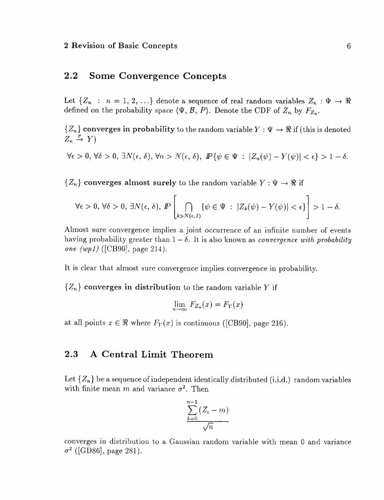
Let {Zn : n = 1, 2, . . .) denote a sequence of real random variables Z, : 9 + 9? defined on the probability space (9, 23, P). Denote the CDF of Zn by Fzn.
(2,) coilverges in probability to the random variable Y : 8 + X if (this is denoted z ,z Y)
\ J f > 0, \ Jb> 0, 3 N ( € , S), \Jn > N ( c , S), P{$E 9 : I&($)-Y(+)l < t) > 1 - 6 .
(2,) converges almost surely to the random variable Y : \I, -t 92 if
Almost sure convergence i n ~ ~ l i e s a joint occurrence of an infinite number of events having probability greater than 1 - 6. It is also k~lown as convergence witlz pl-obability o n e (wpl) ([CB90], pa,ge 214).
It is clea,r that a.lmost sure convergence implies convergence in probability.
(2,) converges in distribution to the random variable Y if
lim Fz, (x) = Fy(x) n-oo
at all points z E 9? where Fl7(z ) is continuous ([CB90], pa.ge 216) .
2.3 A Central Limit Theorem
Let (2,) be a sequence of independent identically distributed (i.i.d.) random variables with finite mean 171 and variance a2. Then
converges in clistributioi~ to a Gaussian rand0111 variable with meall 0 and variance a2 ( [ G D S 6 ] , page 281) .
2 Revisioi~ of Basic Concepts
2.4 The First Borel-Cantelli Lemma
Let {Ak : k = 1, 2, . . .) denote a sequence of events on the probability space (Q, B, P). If CEO P ( A k ) < cc then
P (4 E 9 : 4 E Ak for infinitely many k} = 0.
Consult [Bi179], page 46 for proof and elaboration.
2.5 Stochastic Processes, Sample paths and Separability
A real-valued stochastic process is a collection {Z, : t E T) of real random variables, all defined on a common probability space (Q, B , P). The random variable Zt depends on both t and the point 4 E Q at which it is eva.lua,ted. To empha.size its role as a function of two va.ria.bles, write it as Z($, t ) . For fixed t, the function Z(., t) is a measureable map from 9 into 3. For fixed $, the function Z ( $ , a ) is called a sample path of the stocha,stic process. Consult [PolS4], page 1.
Let A denote a collection of Bore1 sets on the real line. A real stochastic process {Zt : t E T } with a 1inea.r index set T is said to be separable relative to $I if there is a sequence { t j } of parameter values and a subset A c 9 of probability zero such that for any A E A a.nd a,ny open interva,l I, the sets
differ by at most a subset of A. Of particular importance in this paper is that if the class A is taken to be the class of closed sets, then for a separable process, the supremum and infimum over arbitrary intervals are measureable. This is because they agree almost everywhere with the supremum and infimum over countable parameter sets.
2 Revisioil of Basic Concepts
2.6 Metrics, Pseudometrics and L' and L2 Norms.
2.6.1 Metrics and Pseudometrics
A metric for a nonempty set L is defined as a single-valued, nonnegative, real fuilction p : L @ L -t %+ which has the following three properties: For all x, y, z E L,
1. p(x, y) = 0 if and only if z = y;
2. p(x? y) = p(y, x) (syn2metl-y);
3. p(z, s ) 5 p(z, y) + p(y, z ) (trin~z~le i ~ z e ~ v a l i t ~ ) .
A pseudometric is defined si~nilarly except with respect to property (1); for a pseu- dometric, p ( x , y) could be zero for some distinct pair x, y.
A functional p defined on a linear space L is said to be a norm in L if it has the following three properties:
1. p is finite and convex;
2. p(x) = 0 only if x = 02;
3. p(az) = ( a ( p ( z ) for all n: E L a.nd all a.
Recalling the definition of a convex functional, we deduce that a norm in L is a finite filnctional on L such that for a.11 z , y E L,
1. p(x) > 0, where p(x) = 0 if and only if x = 0;
2. p(az) = lalp(x) for all a;
3. ~ ( 3 : + Y) I ~ ( 3 : ) + P(Y)-
2For p an La norm (see later), z = 0 almost everywhere.
2 Revision of Basic Concepts
Let L be a 1inea.r space equipped with a measure p. Then C1 refers to the normed linear spa,ce of all real measurea.ble functions g such that
I ( g 1 1 denotes the L1-norm.
L2 denotes the normed linear space of all real measureable functions such that J g 2 ( x ) dp < m. The C2-norm is defined as
Consult [I<F70], pa.ge 381 for details.
3 On the Uniform Convergence of Relative Fre- quencies of Events to their Probabilities
A synopsis of [VC71] by Vapilik and Chervonenkis
As discussed in the Introduction, the classical Bernoulli theorem states that in a se- quence of 1 i.i.d. trials, the relative frequency of an event A converges (in probability) to the probability of that event as 1 t co [VC71]. The need often arises to ensure that this convergeilce is unifornl over an entire class of events A. In other words, repre- senting the r e h i v e frequency of a set A E A after 1 trials by t,!) and the prol~a~bility of A by PA4, we require that for arbitrarily small F,
IF{?;(') > F) t 0 as l t m, where
The inail1 thread of [VC71] conlprises two strands:
(1) Sufficient conditiolls on A for uniform convergence are derived. These condi- tions do not depend on the probability distribution P, and are discussed in section 3.2. Classes of sets which satisfy these conditions have been dubbed 'Vapnik Chervonenkis (VC) ' classes, [PolSS] or classes of polynomial disc~.imi- nation [PolS4].
(2) Sufficient and necessary conditions for uniform convergence a.re deduced. These conditions do depend on the probability distribution P and are elaborated up011 in Section 3.3.
Before describing these results and their elegant derivations, we need a few supportillg definitions and concepts.
3 Uniform Co~lvergence
3.1 Cake-Cutting, Growth functions and the Shattering of Classes of Sets
3.1.1 T h e Cake-Cutting Coiluildrunl
Any enthusiast for conundra and puzzles is no doubt familiar with the problem of determining, as a function of r , the maximum number of pieces into which a cake E mamy be partitioned using at most r slices. Let us extend the problem to include n-dimensiona,l ca,kes being partitioned by means of r slices ((n - 1)-dimensional hy- perplanes). Denote by @(I?., r ) the nlaximum number of pieces obtainable.
In order to obtain a recurrence relation for Q(n, r ) , consider the case where the first r - 1 hyperplanes ha.ve a.lrea,dy been placed so a.s to maximize the number of compartments into which the 'ca.ke' En ha,s been partitioned. All that remains to be done is to pla,ce the final i.th hyperphne.
Now, for 12 > 2, a.ny two non-parallel (n - 1)-dimensiona,l hyperplanes intersect along an (12 - 2)-dimensiona,l hyperplane. Hence, when the r th hyperplane is inserted, it will be traversed by at most r - 1 hyperplanes, each of which is (n - 2)-dimensional. Further, since the r th hyperplane will form one of the boundaries of any new compart- ments added, the maximum number of new compa.rtments will equal the maximum number of (n - 1)-dimensional segments into which these (n - 2)-dimensional hyper- planes partition the r th hyperplane itself [Wen62], [Sch50]. See Figure 1.
Hence, Q(12, r ) is seen to obey the recurrence relation
@(n, r ) = Q(11., r - 1)+@(1z- 1, r - I ) , where Q(0, r ) = 1 and Q(12, 0) = 1
It is not difficult to show by induction that
and, hence, that for 12 > 0 and r > 0,
In what follows, essential use is nmde both of @(n, r ) and of inequality (3 ) .
3 Uni fo rm Convergence
New compartments
1 -dinunzionol hyp.rplorus intersect
d o q ~ 0 - d t m w u b d h y p . r p h s (points).
Hyperplane 4 is partitioned into O(n-1. r -1 ) = 4
I -dimmwhnal segments by the Uuwe O-dimemdomd hyperplanes (points of intevseclbn). Hence. 4 MU c m n p o d s are odded
Figure 1: 2-Dimensional C a k e be ing pa r t i t ioned us ing 4 one- d imensional hyperplanes. The number of new compartments added by the fourth slice is seen to be @(n - 1, r - 1) = 4.
3.1.2 Fru i t Cakes a n d G r o w t h Funct ions
Let us now consider a slightly different cake-cutting problem. Let there be a set X, of r different fruit chunks scattered throughout the cake En. Denote the positions of the fruit chunks within the cake by xl , 2 2 , . . . , x,.
Instead of a knife with which to tra.ce out hyperplanes, we have a host of implements with which it is possible to extract any one of a class A of cake pieces. Note that A does ,not necessarily delineake a pa.rtition of the cake since the potential pieces of cakes may intersect one another.
Now, each piece A E A picks out or induces the subsample X t of fruit chunks. The problem is to calculate the number of different groupings of fruit chunks which may be extracted by the class A. We term t,his number the index of A with respect to X , and denote it by n A ( x l , x2, . . . , x,). Obviously, A ~ ( X ~ , 22, . . . , x,) is always at most 2', the cardinality of P(X,.). The maximum of n A ( x l , 2 2 , . . . , xr ) over all possible positionings of the fruit chunks is called the growth function and is denoted by m A ( r ) .
3 Uniform Convergence 13
In what follows, we generalize from cakes to any set X. For a more formal definition of the growth function mA(r) , see [VC71], subsidiary definition 1.1.
Example 1: If X is the real line R and A is the set of semi-infinite intervals of the form (-oo, a], a E 32, then mA(r ) = r + 1. [VC71]
Example 2: If X is Euclidean 2-space, E 2 , and A is the set of quadrants of the form (-co, t], t E 32 )2 R, then mA(r ) 5 (r + since there are a t most r + 1 places to set ea.ch of the horizonta,l and vertical bounda.ries [PolS4]. More precisely, mA(r ) = 1 + 5 + f. P PO IS^], problem 11.8).
Example 3: If X is the segment [0, 11 and A is the class of all open sets, then mA(r ) = 2'. [VC71]
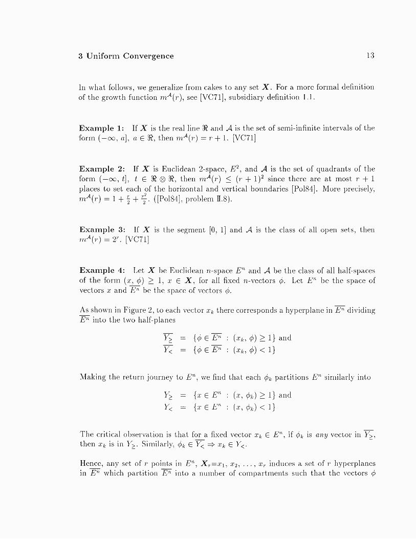
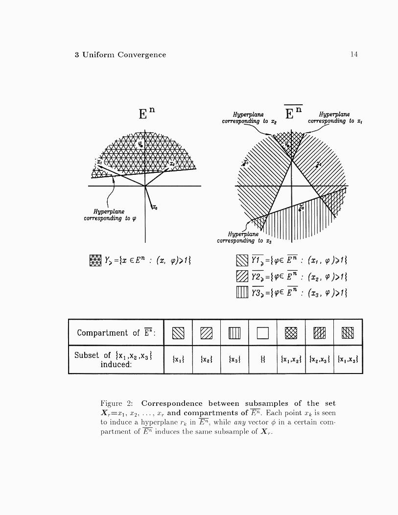
Example 4: Let X be Euclidean n-space En and A be the class of all half-spaces of the form (x, (6) > 1, x E X, for all fixed n-vectors (6. Let En be the space of vectors x and En be the space of vectors (6.
As shown in Figure 2, to each vector xk there corresponds a hyperplane in E" dividing - En into the two ha,lf-pla.nes
- Y> = { ~ E F -
: (xk, (6) > 1) and
Y< = ((6 E En : ( x ~ , (6) < 1)
Making the return journey to E n , we find that each dk partitions En similarly into
Y> - = {x E En : (x, dk) 2 1) and
r/, = {x E En : (x, $k ) < 1)
The critical observation is that for a fixed vector xk E E n , if q5k is any vector in Y>, -
then xk is in Y>. - Similarly, q5k E Y< + xk E Y<.
Hence, any set of r points in En, XT=xl , x2, . . . , x, induces a set of r hyperplanes in E" which pa.rtition En into a number of compartments such tha.t the vectors q5
3 Uniform Convergence
Hyperplane corresponding to p
Figure 2: Correspondence between subsamples of the set XT=xl, x2, . . . , x, and compartments of E". Each point xk is seen to induce a hyperplane r k in E", while any vector 4 in a certain com- partment of E" induces the same subsample of X,.
/ x , I x ~ ~
c o m p a r t m e n t o f F :
Subset of jx, 1x2 .x, I induced: 1 1x2 1 1x3 1 / I I X I , X ~ ~ Ix,sxJ
3 Uniforim Convergence 15
from any single compartment induce half-planes Y> and Y, in E n which, though different for ea,ch 4, all pick out the same subsamp& XY of X,. Thus, finding the growth function for this example is equivalent to finding the lnaximuln number of compartments into which E" may be partitioned, a problem already addressed in Section 3.1.1. i.e. for this example, mA(r) = @(n, r).
3.1.3 Shattering Classes of Sets
A class A of subsets of a universe X is said to shatter a set of points X, c X if it can pick out every possible subset of X, [PolS4]. In other words, A shatters X, if AA(xl, xz, . . . , x,) = 2'. As pointed out in [PolS4], the choice of the term 'shatter' is perha,ps inappropria.te, implying violent fra.gmentation of X, ra.ther than meticulous extraction of each individual subset, ". . . but at least it is vivid" [Po184].
Exainple 5: Consider the c1a.s~ A of closed disks in E ~ : A can shatter any set of three non-collinex points, but cannot shatter any set of four points [PolS4].
All of the above definitions and concepts are elegantly united in Theoreill 1 of [VC71] which states that for any class of sets A, mA(r) is either identically equal to 2' or else is majorized by @(n, r ) , where n is the smallest sample size which A cannot shatter, no matter what the sample configuration (e.g. in Exanlple 5 above, n = 4). In turn, we have shown in Equation (3) that for r > 0, @ ( n , r ) < rn + 1.
Hence, nzA(r) is either equal to 2' or is polynomial in nature, with the order of the polynomial being the value n a.s defined above (For a proof of this theorem, see [VC71]). Classes A for which the latter condition hold are said to be of polynomial discrimination since they pick out at most a polynomial number of subsamples of X,; they have also been dubbed Vapnik Chervonenkis classes in the literature.
We now return to the problem of finding conditions under which we can be assured of uniform convergence of relative frequency to probability over a class A c B of events with respect to the probability space (X, B, P).
To relieve the reader of the torments of suspense, we state the main result of the first part of [VC71] here: It turns out (See [VC71], Corollary to Theorem 2) that a sufficient condition for this uniform convergence to occur is merely that the class of events A be of polynomial discrimination with respect to the whole space X.
This simple result is a consequence of some rather involved yet elegant applications of concepts from ~omhina~torics and pr~ba~bility theory. IVe give here a brief outline of the general argument and refer the reader to [VC71] for the details.
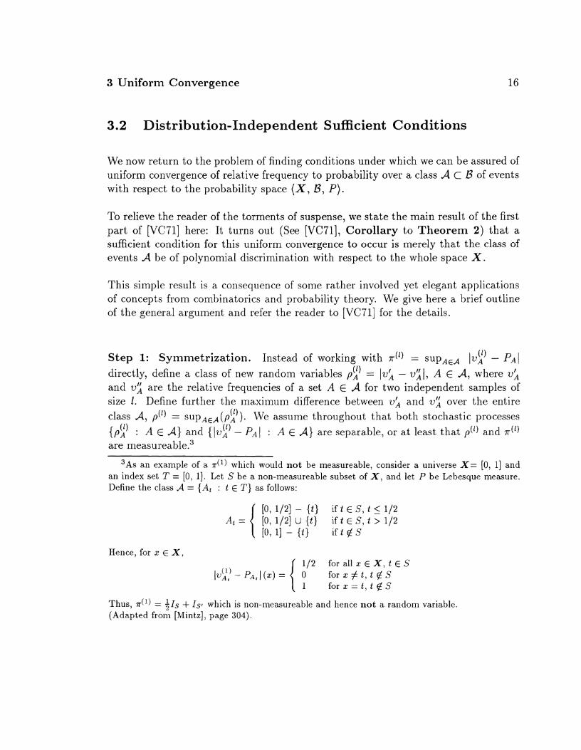
Step 1: Symmetrization. Instead of working with a(') = S U P A ~ ~ lv:' - PAI directly, define a class of new random variables pi' = Iv; - vl;l, A E A, where va and v: are the relative frequencies of a set A E A for two independent samples of size I . Define further the lnaxiinuln difference between v> and vz over the entire
('1 class A, p(') = S L I P ~ ~ ~ ( P ~ ). IVe a.ssume throughout that both stocl~astic processes
{p:) : A E A) and { ~ v t ) - PA ( : 4 E A} are separable, or at least that p( ' ) and r(') are mea~ureable .~
3As an example of a id1) which would not be measureable, consider a universe X= [O , 11 and an index set T = [O, 11. Let S be a non-measureable subset of X, and let P be Lebesque measure. Define the class A = {At : t E T ) as follows:
[O, 1/21 - { t ) if t E S, t 5 112 At = { [o, 1/21 U { t ) if t E S , t > 112
[ O , l ] - { t ) i f t @ S
Hence, for x E X, 112 for all x E X, t E S 0 f o r x # t , t $ S 1 f o r x = t , t @ S
Thus, dl) = +Is + Is( which is non-measureable and hence not a random variable. (Adapted from [Mintz], page 304).
3 Uniform Convergence 17
Lemma 2 of [VC71] establishes that there is a strong relationship between p(') and dl). More precisely,
In other words, if -+ 0 as I + oo, then dl) + 0 (in probability) which is the result we are after. In Step 2 below this type of convergence of is demonstrated for classes A of polynomia,l discrimination.
Step 2: Permutations. Now all that remains to be done is to place bounds on
We note three simplifications which are immediately a.pplicable:
(1) Independence allows us to concatenate the two I-samples used in calculation of va and v: into a single 21-sample, X Z l ,
(2) For a fixed sa,mple X21, inst,ea.d of taking the supremum of IvX -v: I over all of A, we need consider only those sets which induce essentially dzferent subsamples in X,(. Denote the class of all such sets by A'. By definition, IAtI = AA(X21), and
(3) We can partition the cla.ss of all ordered samples of size 21 of the universe X into equivalence classes, each indexed by a subset X c X of size 21, where
[XI = {X,, = T;(X) : i E {1,2,. . . , (21)!))
a,nd Ti is a perlnuta,t,ion of the elements of X.
Hence,
where At depends on the choice of X,[ pursuant to simplification (2) above, and 0 : X 4 { O , 1) is the indicator function for the subset [0, oo) C '$2.
In turn, since the supremum over a class of non-negative functions cannot be greater than the superposition of the functions,
I n [SUP A 6 d 1 ( ( x ~ ) - ) ] d d 5 f l ( ( x ~ ) - ' ) dp AEA' 2
And now for the step which makes use of perm~ta~tions of the sa.lnple X21. Since all samples X2r in a,n equivalence cla,ss [XI generate the same class of sets A', we have
The crucial observation is t.hat the innermost summation represents the total number ( 1 ) of arrangements of a fixed sa~nple Xz1 for which pA > c / 2 . But if A picks out m
( 1 ) elements in XZl, then pA > €12 for any arrangement in which k of these 112 elements N k fall in one I-sample and 12,; - v .4 I = I - - zd I ( 2 €12. Hence, the expression in
brackets, call it I?, may be rewritsten as
Now, since IAtI 5 n2*(21) for all samples XZi and r satisfies I? < we can combine all the rela,tions back to Equation (4) to yield the succint inequality
Finally, for any Vapnili-Chervonenkis class A, mA(21) 5 (21)" so that Inequality (5) implies uniform convergence:
lirn ~ { s ( ' ) > 6 ) < 4 lirn (21)" e-'21/8 - - 0 l i e 2 l i o o
Actually, an even stronger result follows from Inequality ( 5 ) : A simple application of the first Borel-Cantelli Lemma (See Section 2.4) guarantees almost sure convergence. For deta.ils, collsult [VC71].
Note that nowhere in this derivation did we have to iinpose criteria on the properties of the distribution P. This is a testament to the power of the result.
3.3 Distribution-Dependent Necessary and Sufficient Con- dit ions
The second major strand of the [VC71] paper completes the finely woven arras by providing a sufficient and necessa.ry condition for relative frequencies to converge (in probability) to probabilities uniformly over a class of events A.
Since the mathematical justification of the validity of this condition is relatively com- plex and does not lend itself readily to simplification, nor does it contribute to the conceptual clarity of the i d e a , we omit most of it here and refer the reader to [VC71] itself. Instead we lllerely st ate tlie results and discuss their importance.
Once a.ga,in, we need first a definition.
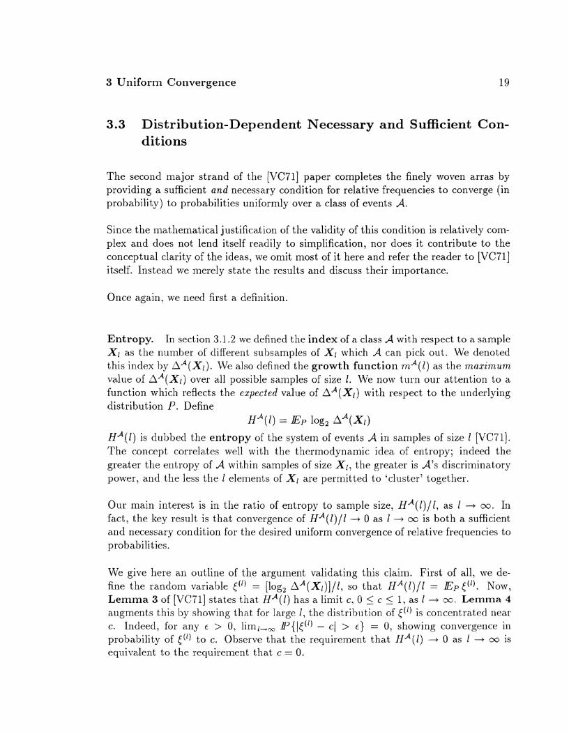
Entropy. In section 3.1.2 we defined the index of a c1a.s~ A with respect to a sample XI a,s the nulnber of different suhsamples of XI which A can pick out. We denoted this index by AA(X1) . We also defined the growth function nxA(l) as the m a x i m u m value of A A ( X ) ) over all possible sa.mples of size I . We now turn our a.ttention to a function which reflects the expected value of A A ( x 1 ) with respect to the underlying distribution P. Define
~ ' ( 1 ) = IEp log, a A ( x 1 )
~ ' ( 1 ) is dubbed the entropy of the system of events A in samples of size I [VC71]. The concept correlates well with the therlnodynamic idea. of entropy; indeed the greater the entropy of A within samples of size XI, the grea,ter is A's discriminatory power, and the less the 1 elell~ents of XI are permitted to 'cluster' together.
Our main interest is in the ra.tio of entropy to sample size, H'(I)/I, a,s 1 t m. In fact, the key result is that convergence of HA(l) / l + 0 a.s 1 t cc is both a sufficient and necessa.ry condition for the desired uniform convergence of relative frequencies to probabilities.
We give here an outline of the argument validating this claim. First of all, we de- fine the random variable ((') = [log, A A ( x l ) ] / l , so that ~ ' ( 1 ) / 1 = Ep [ ( I ) . Now, Leinma 3 of [VC71] states that HA(l) has a limit c, 0 5 c 5 1, as 1 -+ m. Lemina 4 augments this by sl~owing t11a.t for large 1, the distr ibutio~~ of [ ( I ) is concentrated near c. Indeed, for a,ny E > 0, lirnl,, P{\[(') - cl > c) = 0, showing convergence in probability of [('I to c. Observe that the requirement that HA( / ) -+ 0 as I + m is equivalent to the requirement that c = 0.
3 Uniform Convergence
3.3.1 Proof of Sufficiency
To prove sufSricie?zcy of this requirement, let us now partition the space of I-samples XE into two regions: Xf= {log2 A A ( x I ) 5 c21/S) for some t > 0, and XA = X ' - X f . Since these sets are disjoint and exhaustive, invoking elementary set theory4,
Now, by definition, within Xi, A d ( x I ) 5 2P'/8 Further, with c = 0, P (XI) =
P {(('I > r2/8} -t 0 a,s 1 + m by Lelnina 4 of [VCi'l]. Hence, invoking Equation 5 above, we see that
The right hand expression coilverges to zero as I goes to infinity. Hence,
P {a(') > e} i o as i 4 m
3.3.2 Proof of Necessity
To establish necessity of the condition liml,, ~ ' ( 1 ) / 1 = 0, we resort to an argument by contradiction, showing that the supposition limt,, H' ( /) / I = c > 0 implies the existence of a positive r such that. liml,, P{supAEA Ivj4 - v z J > '2s) = 1. A bound similar to Inequality 4, namely
then abrogates uniform convergence of relative frequencies to probabilities. (See [VC71] for details).
Intuitively, this condition imposed on H d ( l ) amounts to ensuring that the expected value of the index of A increa.se at a ra.te strictly sma,ller than the rate of proliferation of subsets of the sample X1 with 1. In other words, even if the growth function mA(l)
*We assume here tha t Xf , X : E B where B is the set of events in the probability space (x', B, P).
increases exponentially, uniforln convergence is assured as long as the expected value of A*(x~) is a member of the o(2') class5.
As a final note, we observe that though this is a fine result, it is attained at the expense of both independence from distribution properties as well as almost surety of convergence. It is shown in [Po1841 that both of these desireable properties may be reinstated with a slight alteration of the condition H ~ ( I ) / I -t 0 as 1 + m. Indeed, Tlleorem 21 of [Po1841 states that a necessary and sufficient condition for almost sure convergence of relative frequencies of events in a class A to their probabilities is ( i z 1 / Z ) f, 0 where nl = n r ( X l ) is the smallest integer such that A shatters no collection of nl points from X l . We refer the reader to [Po184], Section 11.4 and problems lI.11 and lI.12 for a proof of sufficiency and necessity.
5Actually, the conditions are less stringent even than t,his: Thanks t o the concavity of the loga- rithmic function,
H~ ( I ) = I I T ~ log, aA(xl) 5 loga IGP aA(x,) so tha t ~ ' ( 1 ) could still sa.tisfy the criterion even if Ep A*(x,) exhibited expol~e~l t ia l growth.
4 Asymptotics via Empirical Processes
A synopsis of [Po1891 by David Pollard
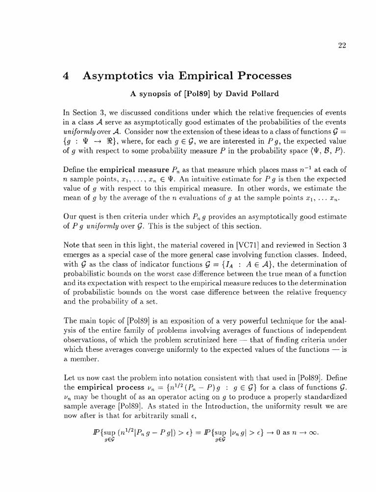
In Section 3, we discussed conditions under which the relative frequencies of events in a class A serve as asymptotically good estimates of the probabilities of the events uniformly over A. Consider now the extension of these ideas to a class of functions G =
{g : Q -+ 81, where, for each g E G, we are interested in P g, the expected value of g with respect to some probability measure P in the probability space (@, B, P).
Define the empirical nleasure Pn as that measure which places mass TI- ' at each of 12 sample points, xl, . . . , z , E Q. .4n intuitive estima,te for P g is then the expected value of g with respect to this empirica,l measure. In other words, we estimate the mean of g by the a.verage of the 12 evalua.tions of g a.t the sa,mple points XI, . . . 2,.
Our quest is then criteria under which Pn g provides an asymptotically good estimate of P g unifol-mly over G . This is the subject of this section.
Note that seen in this light, the material covered in [VC71] and reviewed in Section 3 emerges as a special case of the more general case involving function classes. Indeed, with S as the class of indicator functions G = {IA4 : A E A), the determination of probabilistic bounds on the worst case difference between the true mean of a function and its expectation with respect to the empirical measure reduces to the determination of probabilistic bounds on the worst case difference between the relative frequency and the probabilit,y of a set.
The main topic of [PolSS] is an exposition of a very powerful technique for the a,nal- ysis of the entire faillily of probleins involving averages of functions of independent observations, of which the problein scrutinized here - that of finding criteria under which these averages converge uniformly to the expected values of the functions - is a member.
Let us now casst the prol>lem int,o notation collsistent with that used in [Pol89]. Define the empirical process v, = (P, - P ) g : g E G ) for a class of functions G. v, may be thought of as an operator acting on g to produce a properly standardized sample average [PolS9]. As stated in the Introduction, the uniformity result we are now after is tha.t for arbitrarily sillall E ,
4 Asymptotics via Empirical Processes
The empirical process method for establishing criteria under which the above result holds comprises four main steps [Po189]:
1. Beginning with a family of averages, symmetrize via the introduction of a new source of randomness. Instead of analyzing the difference between an empirical expectation and the true mean, we are now looking at the difference between two independent empirical expectations.
2. Transform the symmetrized process of averages into a conditionally Gaussian stochastic process.
3. Apply a recursive nlethocl known a.s clzaining to exploit the rapid deca,y of Gaussian ta,ils and 1)ound the process proba~bilistica~lly by an integral involving a. capacity function.
4. Derive conditions on the function class S subject to which the necessary uniform bound 011 the capacity function is attained. This bound then percolates through the integra.1 derived in STEP 3 above, and manifests itself as the required bound on the original empirical process.
Figure 3 presents scheinatically the thread of our mini-tour through the labyrinth of empirical processes. In order to present the ma.terial in a modular fashion, we will discuss Ga.ussia,ll Processes and the Chaining method first and then return to the four-step method out,lined al~ove. Though this ordering ma.y seern ha.pha,za,rd, familiarity with Ga.ussia.n Processes and the Chaining method in principle will later obviate the need to break the continuity of the argument with a meandering excursion into clarification of the supporting definitions.
4.1 Maximal Inequalities for Gaussian Processes
As stated in Sectioil L.5, a stochastic process is any collection of random va.riables {& : t E T). A process is mid to be Gaussian if every finite subcollection of these random variables has a joint normal distribution [Po189]. Let us now consider the problem of finding a bound on the expectation of SUPtE~ (Yt( where {x : t E T ) is a Ga.ussian process.
4 Asymptotics via Empirical Processes
Pseudometric p over the index set
of a Gaussian Procm.
Pmbabilistie bound on Probabilistic bound on Probabilistic bound on the maximum over the supremum over the supremum over a
a finite collection of Brownian Molion countable dense subset Normal random vari- (Inequality 7). of a Gautisimn Rocens. abler (Inequality 6).
Probabilirtic bound on co:;t;;ce ':t Probabilistic bound on , an Empirical Process the supremum over a of the involving the capacity Gaussian P m e s
Empirical function (Inquality 11). (Inqualitieti 8 k 0). Process,
Suitable Syrnmetrizatlon. Gousslon Process restrktlons has P -contln~ous
on the capacity sample paths function (1.0. Process is
(kg. MonogeobIlIty of separable). distribution class)
Figure 3: Scl~ematic of the maill thread through the labyrinth of elmpirical processes.
4.1.1 Finite Collectiolls of Normal Random Variables
Consider first the rela,ted problem of estimating the maximum of a finite collection of normal random variables {Zi N N(0 , a:) : i = 1, . . . , n ) where nothing is known about the joint distributions. Define a = max (ol, . . . , an ) . A crude bound on maxi (Zi( is Cy=l IZ;]. Since
we conclude that -
The problem with this bound is that we have placed identical emphasis on the con- tribution of each (Z;I towards C:="=,ZiI. In order to improve on this bound, we need somehow to stress the contribution of whichever lZil is the t r u e maximum, while si- multaneously suppressing the contributions from the other JZ;J's a.s much a,s possible.
We do this by transforming the (Zi17s via a nonnegative, convex, increasing function A4(-) on the positive half-line:
4 Asymptotics via Empirical Processes 25
From Jensen's Illequality (see Section 2.1) followed by the crude bound,
In order to exploit convexity as much as possible, we make H increase as fast as the tails of IZiI can bear without allowing the sum of expectations lP M (1Z;l) to exceed a multiple of n [PolS9]. It is straightforward to show that for normal tails, the function h.f(r) = ex2/4"2 suffices to ensure that P M (1Z;I) < \/i for all i. Thus,
PM(JZi1) < M-' [ h n ] < M-' [n2] < 21/50 (logn)lI2 for n > 2, i = l I
whence P max jZiI < 3 m+x 0; (log n)'I2 for n > 2. (6) Z Z
The chaining method of Section 4.1.2 makes use of repeated applications of Inequal- ity (6) to obtain a. surprisingly good bound on the supremum of a Gaussian process.
4.1.2 Brownian Motion and Chaining
Before addressing Gaussian processes in their full generality, consider next the special case of Brownian hlotion on the bounded index set [O, S].
Browiliall Motion or the Wiener Process on [O, 51 is defined to be a Gaussian process {B(t ) : 0 5 t 5 6) with the following properties ([Bi179], page 442):
1. With probability 1, B(0) = 0 (Process begins at the origin).
3. For any t , s E [0, S], the iilcrement B(t) - B(s ) is distributed N ( 0 , It - s J ) .
Once a,gain, we a.re intere~t~ed in a ljound on t,he expectja.tion of suptcp, ,] IB(t)l. The main idea, of the chaining method is to approximate this supremum by the maximum
4 Asymptotics via Empirical Processes 26
taken over a succession of finite subsets of [ O , 61 each more finely spaced than the last. For k = 0, 1, . . ., define Sk = S/2' and let T(k) denote the set of 2k equally spaced points {Sk, 2Sk, . . . , 2'Sk). Owing to sample path continuity, the lnaxiinum of B( t ) taken over T(k) increases monotonically to sup,,[,, I B( t ) 1, whence
IF' max IB(t)l + IP sup IB(t)l as k -, oo. t€ t (k ) tE[O, 4
Figure 4 represents a systematic way of relating the maxima over successive sets T(k). In a, way, the hunt for the supremum of B(t) is akin to a pa.ra.lle1 binary tree-sea.rch over [0, S]. The crucial observation is that for any k > 1, to each t in T(k) there corresponds a t' in T(k - 1) at most a distance of Sk-l away. Thus, for each t, t' pair, by the triangle inequality,
IB(t> l 5 IB(t') l + IB(t) - B(tl)l.
So, when atte~llpting to find the maximum of IB(t)l over a set T(k), k 2 1, one need only find the maximum over the set T(k - 1) and then add to this value the maximum discrepancy maxt~~(k), t l~T(k-1) I B ( t ) - B(t1) 1 :
max IB(t)l 5 , yyl) IB(tt)l + max IB(t) - B(tt)1 t € T ( k ) t € ( , - t € T ( k )
Now, for Brownian Motion, each increment B(t) - B(t1) is distributed N(0, Sk), so tha,t,, by Inequality (6), P maXtE~(k) IB(t) - B(tr)l 5 3~:?~(1o~ 2')lf2. Hence, taking expected values of both sides of the above inequality yields the recurrence relation
P ma,x IB(t)l P max 18(t)1+3\/6i.-ll0g2~, t€T(k ) t€T(k-1)
P max I B(t) ( = P 1 B(S)I t€T(O)
whose solution is k
P max I B ( ~ ) I 5 P IB(S)~ + ~3 Ja. t € T ( k ) i=l
Hence, making use of the identity Si = S;-1/2, i > 1 and the fact B(S) N N(0 , S), and letting k 4 m,
1 ~ ( t ) 5 &PIN(O, 111 + A 53di (:)i-l log 2 t€[o,S] i = l -
5 I<J& since the infinite sum converges.
4 Asymptotics via Empirical Processes
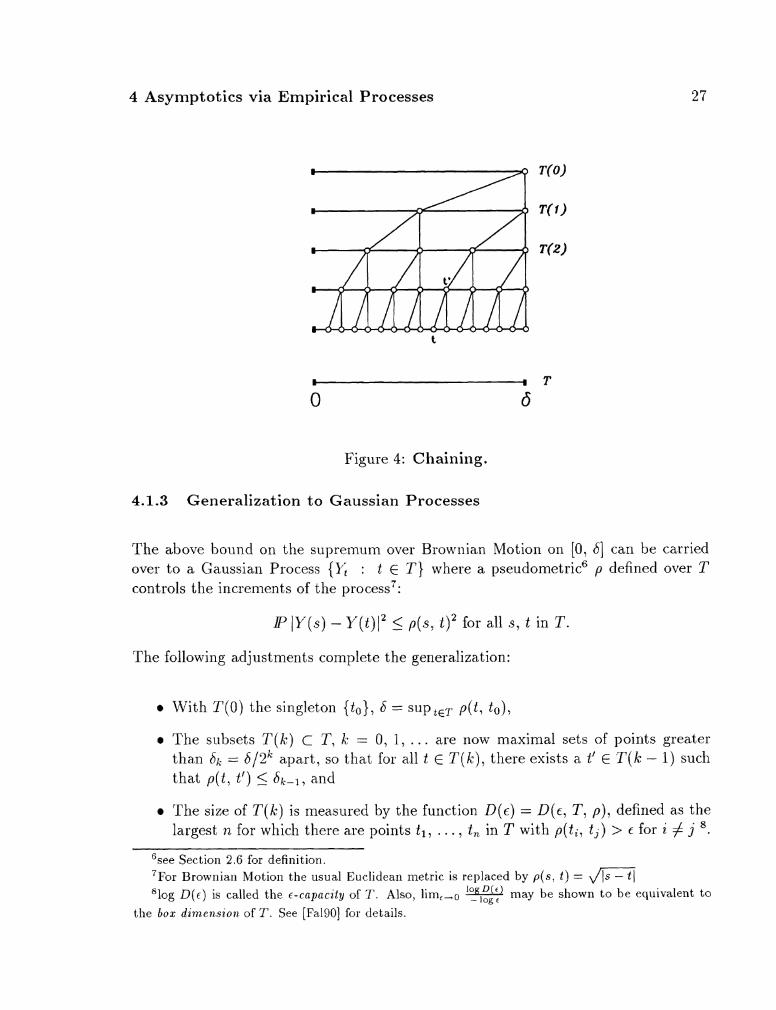
Figure 4: Chaining.
4.1.3 Geileralization to Gaussian Processes
The above bound on the suI>remunl over Brour~lian Motion on [0, S] can be carried over to a Gaussian Process {I: : t E T ) where a pseudometric6 p defined over T controls the increments of the process7:
P IY(s) - y ( t ) I 2 5 p(s, t j 2 for all s, t in T .
The following adjustments complete the generaliza,tion:
r With T(0) the singleton { to} , S = SUPtET P( t , to):
r The subsets T ( k ) c T , k = 0 , 1 , . . . are now maximal sets of points greater than sii = S/2".l~art, so that for all t E TJX-), there exists a t' E T(k - 1) such tha,t p( t , t ' ) 2 Sk-lr a.11~1
r The size of T ( k ) is measured b y the functioll D(c) = D(6, T , p ) , defined as the largest n for which there are points tl , . . . , t , in T with p(t i , t j ) > 6 for i # j
'see Section 2.6 for definition. 'For Brownian Motion the usual Euclidean metric is replaced by p ( s , t ) = 'log D(r) is called the r-copnt i fy of T. Also, lirn,-o may be shown to be equivalent to
the box diinei~sion of T. See [Fa1901 for details.
4 Asymptotics via Empirical Processes 2 8
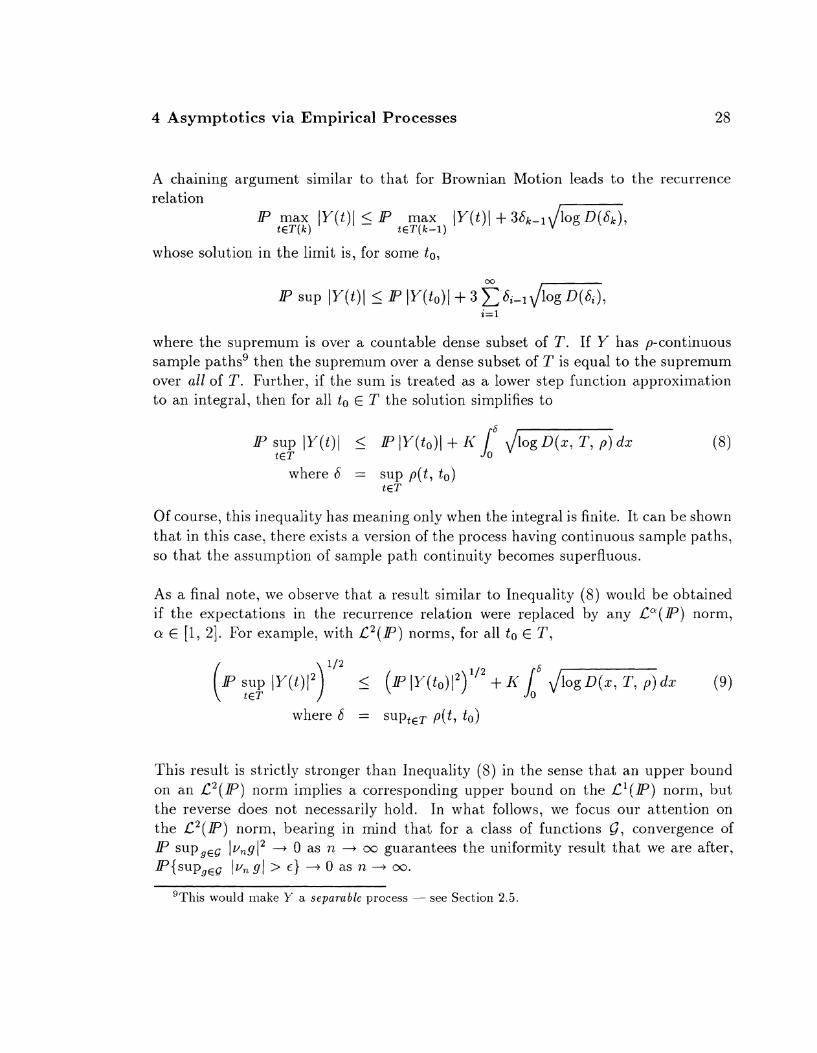
A chaining argument similar to that for Brownian Motion leads to the recurrence relation
P max IY(t)l 5 P max I Y ( t ) 1 + 3 6 k - l J a , t€T(k) t€T(k-1)
whose solution in the limit is, for some to,
where the supremum is over a countable dense subset of T. If Y has p-continuous sample pathsg then the supremum over a dense subset of T is equal t o the supremum over all of T. Further, if the sum is treated as a lower step fuilction approsimatioil t o an integral, then for all to E T the solution simplifies to
P sup lY(t)l < P I Y ( t o ) l + r c / - ~ l o g ~ ( x , T , p)dz t€T 0
(8)
where 6 = sup p(t, t o ) t€T
Of course, this inequa.lity has mea.ning only when the integral is finite. It can be shown that in this ca.se, there esist,s a version of the process having contiiluous sa,mple paths, so that the a.ssumption of sample path continuity becomes superfluous.
As a final note, we observe that a result similar to Inequality (8) would be obtained if the expecta.tions in the recurrence relation were replaced by any C f f ( P ) norm, a E [I, 21. For esa.mple, with C 2 ( P ) norms, for all to E T,
where S = SUPtc~ p(t, to)
This result is sttric,tly stronger t11a.n Ineclua,lity (8) in the sense that a.11 upper bound on an L 2 ( P ) norm implies a corresponding upper bound on the C 1 ( P ) norm, but the reverse does not necessarily hold. In what follows, we focus our attention on the C 2 ( P ) norm, bearing in mind that for a class of functioils S, convergence of P supgEc 1vn9I2 -+ 0 as n -+ co guarantees the uniformity result tha,t we are after, P{supgEG lv, gl > c} + 0 as n -+ oo.
'This would make Y a separable process - see Section 2.5.
4 Asymptotics via Empirical Processes
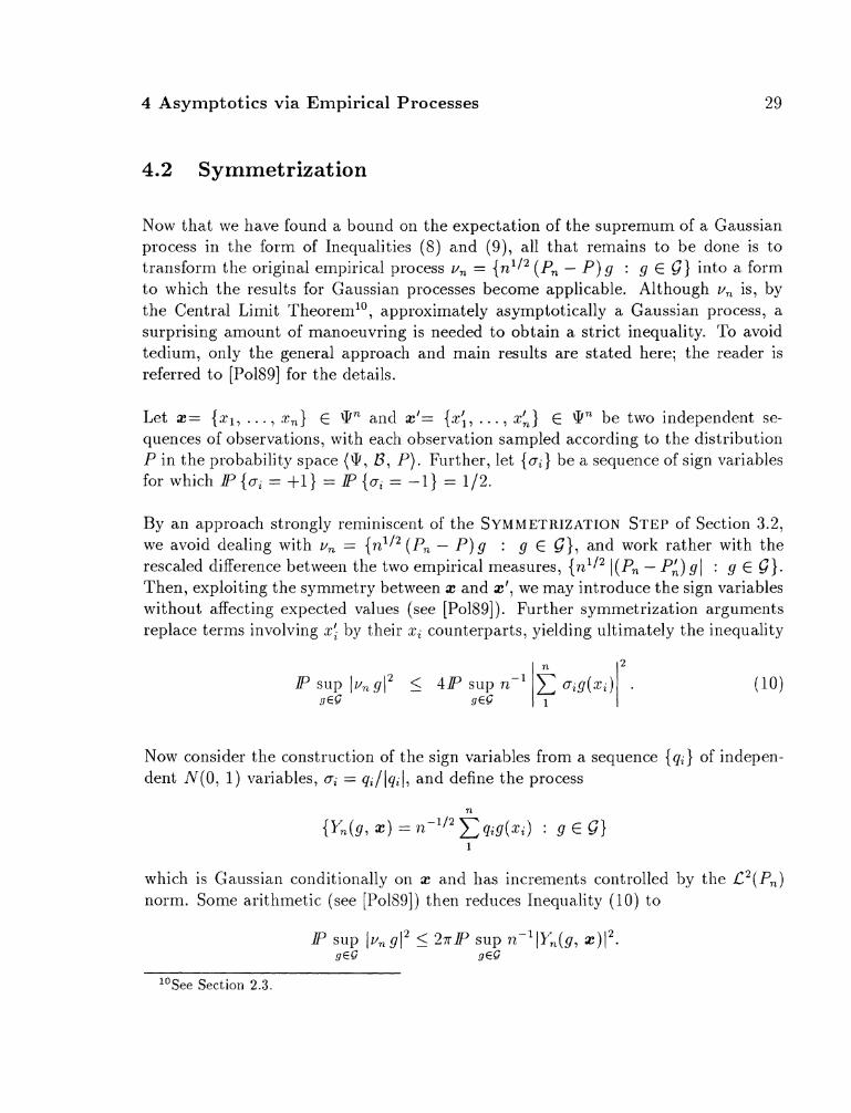
4.2 Symmetrization
Now that we have found a bound on the expectation of the supremum of a Gaussian process in the form of Ineclualities (8) and (9)) all that remains to be done is to tra,nsfornl the original empirical process v, = in1/' (P, - P) g : g E G ) into a. form to which the results for Gaussian processes become applicable. Although v, is, by the Central Limit Theorem1', approximately asymptotically a Gaussia.n process, a surprising amount of manoeuvring is needed to obtain a strict inequality. To avoid tedium, only the general approach and main results are stated here; the rea.der is referred to [Pols91 for the details.
Let x = {zl , . . . , x,) E Qn and xl= {xi, . . . , x:) E 9" be two independent se- quences of observations, with each observation sampled a,ccording to the distribution P in the probability space (Q, B , P). Further, let {a;) be a sequence of sign variables for which P {ai = $1) = P {a; = -1) = 1/2.
By an approa,ch strongly reminiscent of the SYMMETRIZATION STEP of Section 3.2, we avoid dealing with v, = {7z1I2 (Pn - P ) g : g E 6)) and work rather with the rescaled difference between the two empirical measures, {nl/' ((P, - PA) gl : y E G}. Then, exploiting the symrnetry between a: and a:', we may introduce the sign variables without affecting expected values (see [Po189]). Further symmetrization arguments replace terms involving z: by their z; counterparts, yielding ultimately the inequality
Now consider the construction of the sign variables from a sequence { q ; ) of indepen- dent N(0 , 1) variables, a; = q;/ [q;l, and define the process
which is Gaussian conditionally on a: and has increments co~ltrolled by the L2(Pn) norm. Some arithmetic (see [PolS9]) then reduces Inequality (10) to
P sup (v,,gI2 5 2nP SUP 72-'1Yn(g, x)I2. s € B s€B
''See Section 2.3.
4 Asymptotics via Empirical Processes
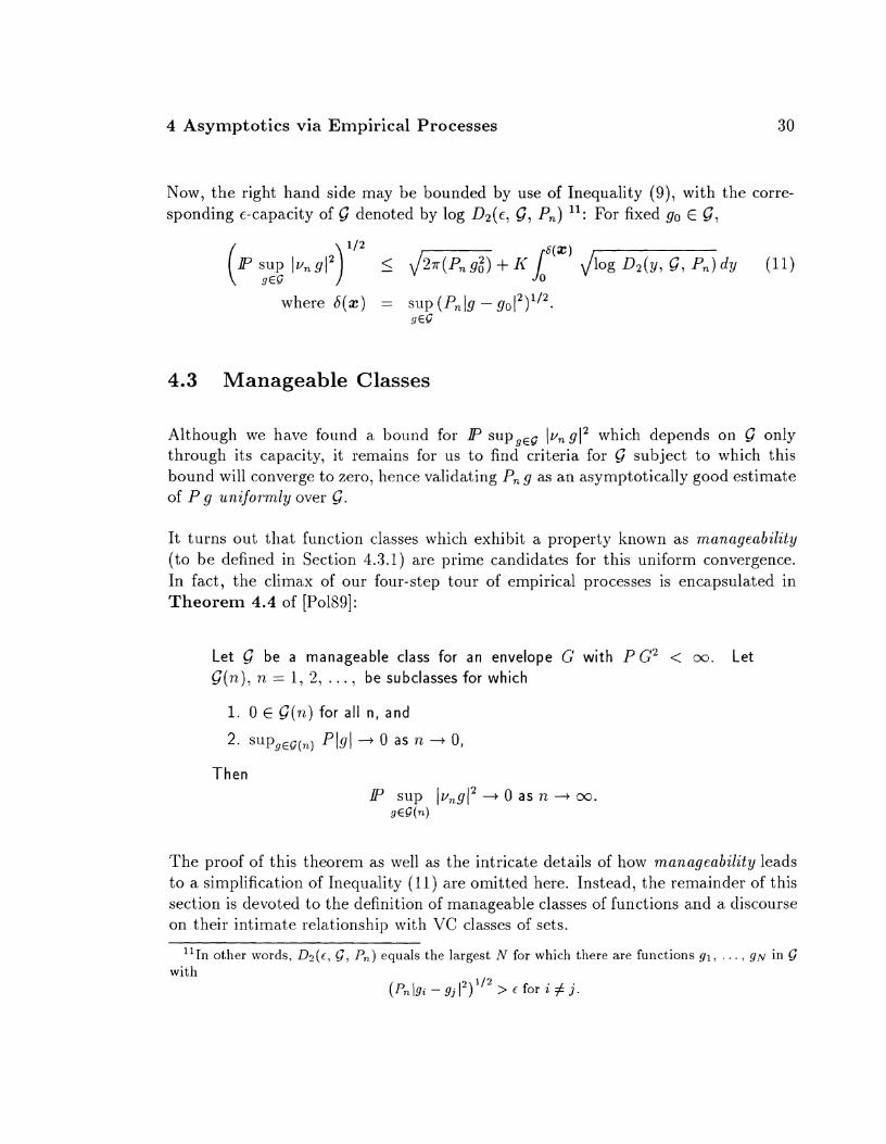
Now, the right hand side may be bounded by use of Inequality (9), with the corre- sponding €-capacity of G denoted by log D'(E, G, Pn) 11: For fixed go E G,
2 112 where S ( X ) = s u p ( P n l g - g ~ l ) - sEG
4.3 Manageable Classes
Although we have found a bound for 4' supgEG (u,,gI2 which depends 011 Q only through its capacity, it remains for us to find criteria for G subject to which this bound will converge to zero, hence validating Pn g as an asymptotically good estimate of P g uniformly over G .
It turns out that function classes which exhibit a property known as manageability (to be defined in Section 4.3.1) are prime candidates for this uniform convergence. In fact, the climax of our four-step tour of empirical processes is encapsulated in Theorem 4.4 of [PolSS]:
Let S be a manageable class for an envelope G wi th P G 2 < cm. Let
G ( 1 2 ) , 12 = 1, 2 , . . . , be subclasses for which
1. 0 E G ( n ) for all n, and
Then IP sup IvngI2 -+ 0 as n -t m.
S E P ( ~ )
The proof of this theorem as well as the intricate details of how manageability leads to a simplification of Inequality (1 1) are omitted here. Instead, the rema,inder of this section is devoted to the definition of manageable classes of functions and a discourse on their intimate relationship with VC classes of sets.
l l l n other words, & ( E , G , P,,) equals the largest N for which there are fuilctions y l , . . . , g~ in with
4 Asymptotics via Empirical Processes
4.3.1 Definition of Manageability
Let 6 be a class of functions with envelope GI2. 6 is said to be manageable for G if there exists a decreasing function D(.) for which
1. 1' J m d r < ca, and
2. for every measure Q with finite support,
D2 (em, 6, Q) 5 D(c) for 0 < c < 1.
It is seldom possible to calculate directly the uniform bound on capacities required by this definition [Pol89]. How, then, are we to establish manageability of a function class and hence exploit the results of the previous section? The answer to this cluestion involves VC classes of sets and is perhaps as remarkable as it is elegant.
4.3.2 VC Classes of Sets and Manageable Classes of Functions
Define the subgraph of a function g : 6 -+ % as a subset of the product space Q @ 8:
Define also a Euclidean function class as a class with envelope G for which, for measures Q of finite support,
sup Dl(cQG, 6, Q) = o(E-') for some V , Q
where Dl is the L1(Q) capacity of 6.
The crucial connection between VC cla.sses, subgraphs and Euclidean functioil classes appears as Lemma II.25 of [PolS4]:
1 2 ~ h a t is, G' 2 l g ( for every g E 5'
4 Asymptot ics via Empirical Processes 3 2
Let G be a class o f functions on Q wi th envelope G, and let Q be a measure on Q wi th finite support. If the class of subgraphs of functions in G fo rm a VC class o f subsets o f Q @I %, then 6 is Euclidean.
From here, the final leap is easy: Elementary inequalities involving the L 1 ( P ) and L2(Q) seminorms, where P has density G with respect to Q, show that Euclidean classes of functions have analogous bounds on their L2 capacities ([Po184], Leinma 36). In particular,
Every Euclidean class is manageable.
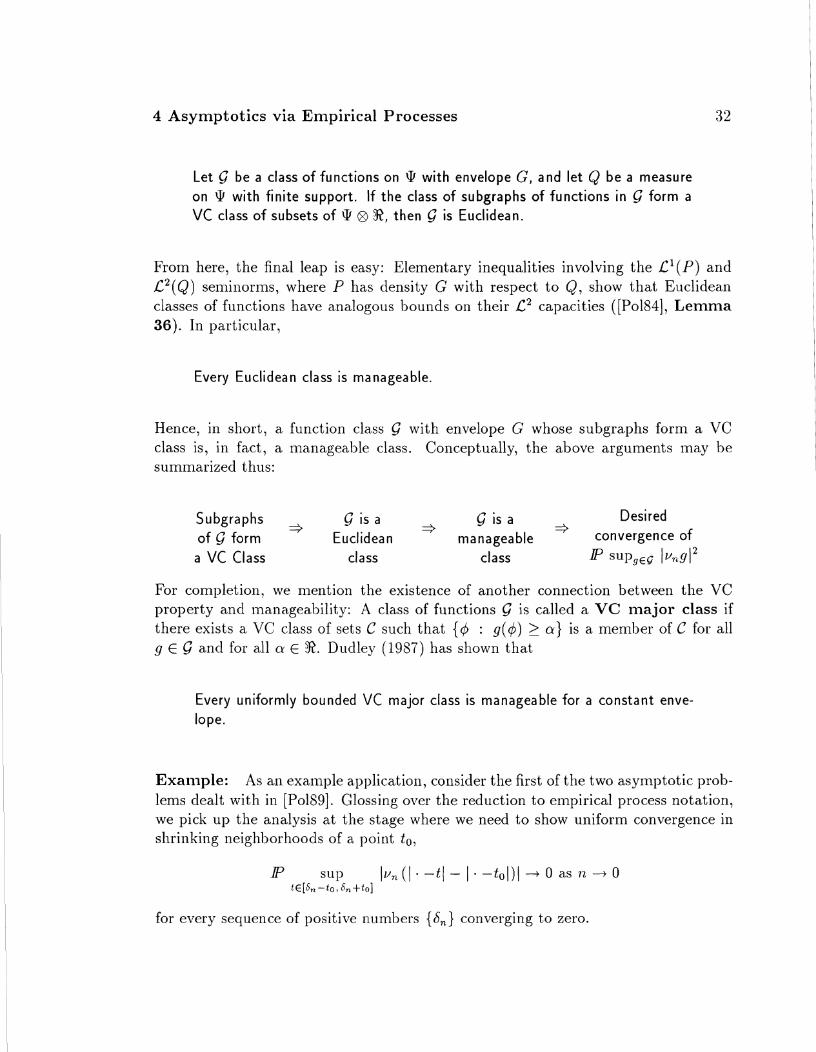
Hence, in short, a, function class G with envelope G whose subgraphs form a VC class is, in fact, a managea.ble class. Conceptually, the above arguments may be summarized thus:
Subgraphs + G i s a S is a Desired =+
o f G fo rm Euclidean manageable * convergenceof
a VC Class class class S U P g ~ ~ /~ ,91 '
For completion, we nlention the existence of another connection between the VC property and manageability: A class of functions 6 is called a VC ma jo r class if there exists a VC class of sets C such that {q5 : g ( 4 ) 2 cr} is a member of C for all g E 6 and for all CY E %. Dudley (1987) has shown that
Every uniformly bounded VC major class is manageable for a constant enve- lope.
Exanlple: As an example application, consider the first of the two asymptotic prob- lems dealt with in [Pol89]. Glossing over the reduction to empirical process notation, we pick up the analysis at the stage where we need to show uniform convergence in shrinking neighborhoods of a point to,
P sup Iun ( 1 , -tl - I . -tol)l -t 0 as n -+ 0 t € [ S n - t o , & + t o ]
for every sequence of posit,ive numbers (6,) converging to zero.
4 Asynlptotics via Enlpirical Processes
Consider a member y(., t ) of the function class 6 = {g( . , t ) = ( I -t( - I -tol) : It, - t ( 5 6,). It has a constant value of t - to on the interval (-oo, min{t, to}], a constant value of to - t on (max{t, to), oo, 1, and inbetween follows the straight line joining (t - to) to (to - t).
Hence, for any a E X and t E [&-to, &,+to], the inverse image C = {x : g(z , t ) 2 a ) is a semi-infinite interval on the real line. Now, the class C of all such intervals has been shown in Section 3.1.2 to be a VC class. Thus, is a uniformly bounded VC major class, and is, therefore, manageable for co~lstant envelope S1.
Furtller, g(to, to) = 0 E G and for all g E S, P g < It - to1 I bn + 0 n -+ 0, whence all the hypotheses of Theorelm 4.4 of [Pol891 (see Section 4.3) are satisfied. It follows tha.t uniform convergence is, indeed, a.ttained.
4.3.3 Properties of Manageable Classes
We coilclude this chapter with a few subsidiary remarks about the nature of manage- ability, and the construction of more complicated manageable classes once the basic classes have been established by way of VC classes of subgraphs or VC major classes of functions.
The first three of the following properties of manageable classes are deduced from elementary L2 inequalities; the reacler is referred to [Po1891 for a sample derivation. The last property is taken from Dudley (1987), Theorem 5.3.
If S is manageable for envelope G and 'FI is manageable for envelope H , then
1. Go3-1 = { y o h : g E S, h E 3-11 is manageable for envelope G + H , where the symbolic operator o represents addition (+), maximum (v), or minimum (A).
2. S* 'FI = {gh : g E 6, h. E 3-11 of products is manageable for envelope G H .
3. The closure of S under convergence is manageable for envelope C:
4. The symmetric convex hull o f G , denoted by sco(S) and consisting of all f inite linear combinations C ajg j of functions gj E G for which
C \ail 5 1, is manageable for envelope G.
5 Geometrizing Rates of Convergence
A synopsis o f [DL911 by Doiloho and Liu
As mentioned in the introduction, any discussion on asymptotics must go hand in hand with a treatment of rates of convergence. The theme of [DL911 revolves around a bound on the ra,te of convergence of an estimate Tn(Xn)13 to the value of a functional T ( F ) of an unknown distribution F E F uniformly over a class of distributions F. The main result is two-fold: First, it turns out that for estimating a linear functional over a convex distribution class F, the geometry of the problem, expressed in terms of an index known a8s the ~nodu1,us of continuity b ( e ) , determines the optirnal ra,te of convergence. Second, and per11a.p~ Inore startling, is that this optimal rate is, in fact, attainable, provided only that b ( e ) is Holderian14.
The result is estal~lished by way of allother bound on the rate on convergence, denoted by AA and involving the difficulty of testing the composite hypothesis15 Ho : T ( F ) 5 t against the composite hypothesis HI : T ( F ) > t + A. Under certain asymptotic con- ditions, AA is altoays attainable, to within constants, regardless of the characteristics of the functiona.1 T or the class of distributions F . Linearity of T and convexity of F then guarantee t1la.t the modulus bound agrees with AA, to within constants. From here, verification that b ( ~ ) is a. Holder function is all that is necessary to ensure tha,t the supporting asymptotic conditions are met.
Yet that is not all. DonohokLiu show that for the modulus bound to agree with AA, the prerequisites of linea,rity and convexity may be discarded, provided that the essence of the geometry is preserved: A new criterion is that the hardest two-point subproblem of testing T ( F ) 5 t versus T ( F ) > t + A should be roughly as difficult, from a mi11ima.x risk point of view, as the full conlposite hypothesis-testing problem. Moreover, in one example, DonohokLiu show that even this last condition may be dropped. On the other hand, in all cases satisfaction of a Holder condition by the modulus of continuity is necessary in order to preserve the attainability of the optimal rates. For clarity, the relationships ainong these concepts are shown graphically in Figure 5 .
In this section, we review the definitio~ls and properties of concepts vital to later developments. We then identify AA(iz, a ) as a lower bound, to within constants, on the rate of convergence of T,(X,) to T ( F ) (Theorem 2.1 of [DLgl]). Next, we
13where X, is a vect,or of n i.i.d. F sample poiilts 14See Section 2.1 for definition. 15See [CB90], Sectmion 8.3, for a. very lucid treatment of Hypothesis testing.
5 Geometrizing Rates of Convergence
Tho kmrn uppw \
d a of mlnlmax rlsk cmwrgmnca to zoro
u n d a 0-1 h. SoH~focHon of ([DUl]. Theorom 2.1) orymptoflc
conditions k r b d h Inquolily 12.
UM~* of 1.
A, = b(c1h)= a("*) b oltdnoblr and b,
m a u p p r b w n d b Ilu optlmol mtr of on lh. mf. of mhlmm mrmr(lrwr d M
o h ond oshahuT, blh.
hndbml 1. blow t b
roughly 0s dlfflcun as full
compoaih pmblmn.
Thr 2-polnt losling bound, AZ. 1s H d f
boundad o h and b o h by Ih. modulus
of conilnully* Me) ([DLOl]. hmma 3.2).
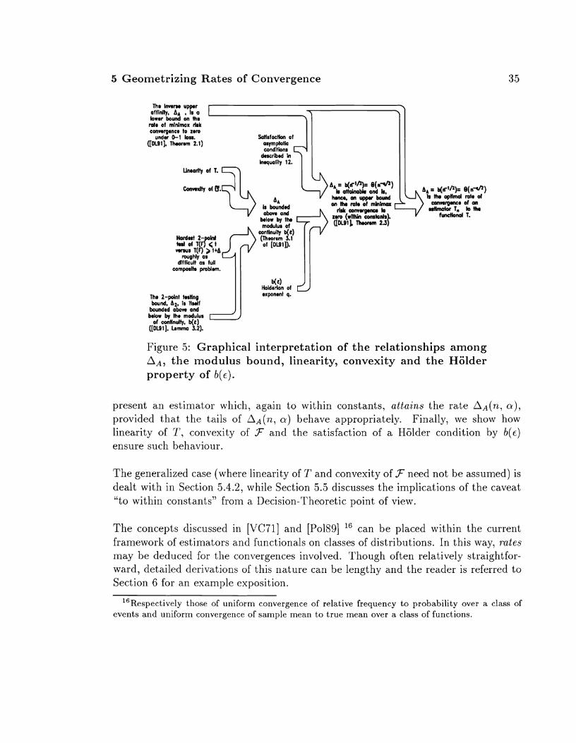
Figure 5: Graphical interpretation of the relationships among AA, the ~nodulus bound, linearity, convexity and the HSlder property of b ( c ) .
present an estima,t'or which, again to within constants, attains the ra.te AA(n, a ) , provided that the tails of aA(n, a ) behave appropriately. Finally, we show how linearity of T, convexity of F and the satisfaction of a Hijlder condition by b ( e ) ensure such behaviour.
The genera.lized case (where linearity of T and convexity of 3 need not be a,ssumed) is dealt with in Section 5.4.2, while Section 5.5 discusses the implications of the caveat "to within constants" from a Decision-Theoretic point of view.
The concepts discussed in [VC71] and [Po1891 l6 can be placed within the current framework of estima,tors a.nd functiona.1~ on cla,sses of distributions. In this way, rates may be deduced for the convergences involved. Though often relatively straightfor- ward, detailed derivations of this nature can be lengthy and the reader is referred to Section 6 for an example exposition.
16~espectively those of uniform convergence of relative frequency to probability over a class of events and uniform convergence of sample mean to true mean over a class of functions.
5 Geometrizing Rates of Convergence
5.1 Definitions
The following definitions are concerned with the distinguishability of distributions within a class a.nd the difficulty of estimating a functional T over such a class.
5.1.1 Hellinger Affinity
Hellinger Affinity p(P, Q ) is a measure of the 'closeness' of two measures P and Q and is defined as ,-
where p = Q , q = 2 for any measure p which dominates P and Q [LY90]. d~
5.1.2 Hellinger Distance
The Hellinger Distance H(P, Q ) between two probability measures P and Q is defined as
where, as before, p = $, g = 2 for any measure p which dominates P and Q [LYSO].
It can easily be shown that
H'(P; Q) = 2 (1 - P(P, Q ) )
5.1.3 Modulus of Continuity
The modulus of continuity of a functional T over a class of distributions F, with respect to Hellinger dista,nce, is defined as
b ( ~ ) = SUP { I T ( F I ) - T(Fo)l : H(F1, Fo) 5 E , Fl, Fo E F}.
In words, the ~noclulus of continuity measures, as a function of c, the greatest variation of the functional over any Hellinger ball of radius c. In a way, it gives an indication of
5 Geometrizing Rates of Convergence
the extent of correlation between the "shape" of a distribution and the value of the functional of that distribution: For functionals which exhibit very little dependence on how the probability mass is distributed17 and can change wildly for very similar (in a Hellinger sense) distributions, the modulus will be large, even for small 6. On the other hand, functionals which are highly dependent on mass distribution1' will tend to have small moduli, perhaps linear or polynomial in 6 for 6 + 0.
Throughout the remainder of this paper, we will be interested in the asymptotic behaviour of b(c) for 6 t 0.
In order to build up some intuition rega,rding the nature of the modulus of continuity, we look at a few examples of f~inctionals and classes of distributions and derive their moduli.
Example 1: Location Parameters. Consider the class of shifted Gaussian dis- tributions F = { N ( u , 1) : a E S R } and a functional T which returns some location parameter such as the mean. Let Fo and Fl be distributions whose loca,tions differ by A > 0. Then the Hellinger affinity between Fo and Fl is seen to be
Thus the Hellinger dista,nce between the two distributions is
Since this is a moilotonically increasing function of A, we see that in any Hellinger ball of radius 6, the distributions whose locations are furthest apart lie on the skin of the ba,ll. Hence, the modulus of continuity is simply the inverse function of the Hellinger distance:
A Taylor Series expansion of the above yields b(6) = 2f + f + O(c5), whence it is clear that b(6) is dominated by the linear term for E t 0.
'?Consider, for instance, a functional which counts the number of local maxima in the probability density.
l%ucl~ as 11lea.n or 1nedia.n.
5 Geonletrizing Rates of Co~lvergellce
In a similar fashion we may show that the modulus is linear for location parameters over classes of Laplacian or Cauchy distributions:
In the case of Laplacians, .F = {F(.) = J1, e-lt-al/2 dt : a E W) so that some algebra leads to p(FO, Fl) = 3, where, as before, the locations of Fo and Fl
differ by A 2 0. Hence, H(FO, Fl) = Jw which, once again, is monotonically increasing. Some numerical analysis then confirms that b ( ~ ) , the function inverse of H, is dominated by a linear term for small E.
The case of Cauchy distributions yields similar calculations.
Example 2: A Nonlinear Modulus. Consider the problem of estimating the value of a density at a point. [Far721 deals with optimal rates of convergence in a very general setting. In this exa.niple we limit our a,nalysis to a very specific class of distributions, and show that in this case, the modulus of continuity is quadratic for small 6 .
The main idea is to choose a class of distributions for which minor differences in the value of the functional are amplified in the profiles of the densities concerned. Hence, distributions which are confined t,o small Hellinger balls must have very similar profiles, and even closer f~ulctional values.
We select the class of densit,ies indexed by a E (0, 11 where a,n arbitrary member f , is defined by1':
J a a & for 0 5 T 5 n where c l x = l + n = 1 + - 0 J ' ( ;J2-1
fa(x) =
0 elsewhere
Let the functional be T(F,) = F,(O) = a. Let us now calculate the Hellinger distance between two arbitrary members F, and Fp of F = {F,(.) = Jl, f,(x) dx : a E (0, 11). Without loss of generdity, assume a > P. Hence,
lgPer l~aps unexpectedly, the rate of decay of the tails of these types of densities does not seem t o i~lflueilce the modulus of continuity. For instance, identical results are obtained if we choose f,(r) = iz+;lll., or eve11 f,(r) = ;e-"", where n t (1, cc) and 0 < r < o for a suitably
normalizing a.
5 Geometrizing Rates of Convergence 3 9
Substituting y = x + 1,
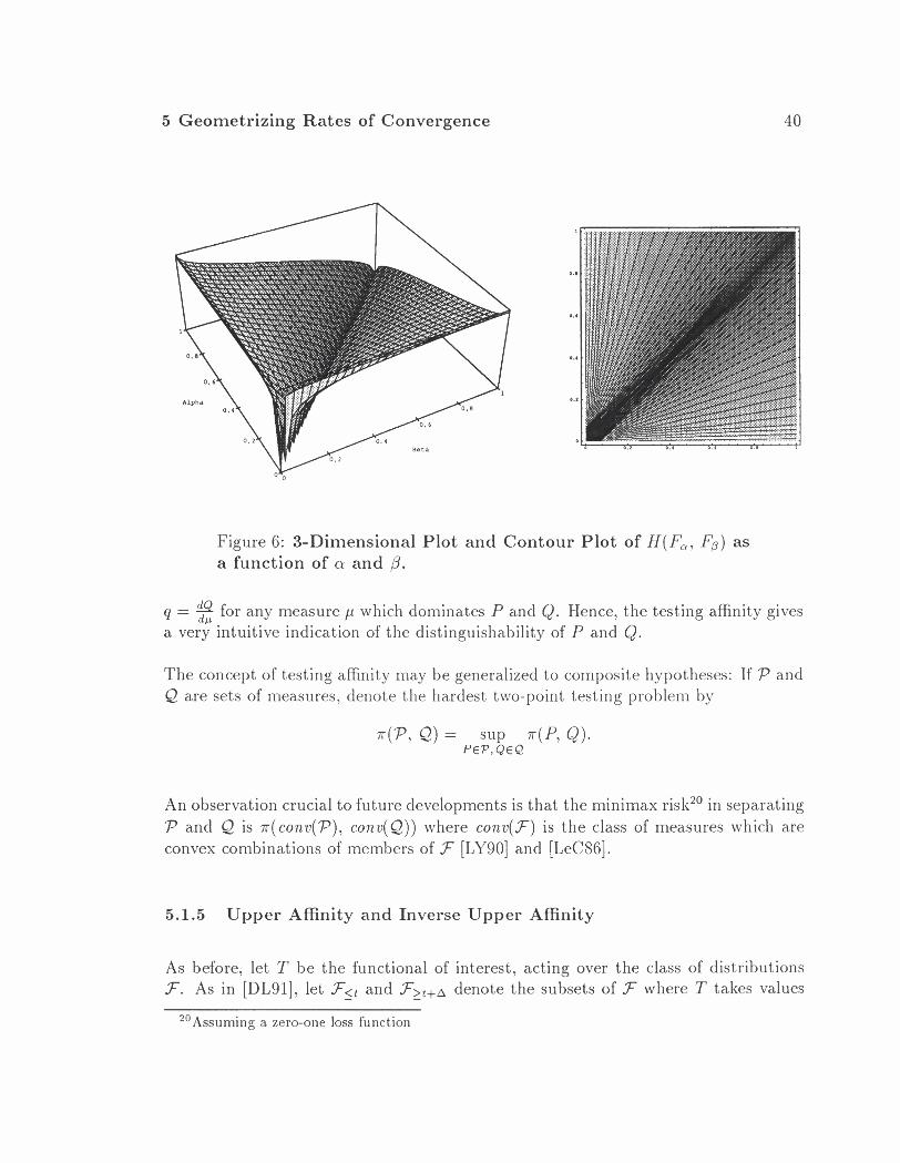
Plotting H(F,, F p ) a.s a f~~nc t ion of cr and /? yields the surface in Figure 6. Contour lines represent the skins of Hellinger ba.lls, so tha,t from Figure 6 we see t11a.t for any Hellinger ball of radius &, the difference between cr and P is lnaxilllized on the skin of the ba,ll at CY = 1 2 J . Hence we can derive the modulus of continuity: For any O S & < l ,
= H(FI. F I - ~ . ) ) = JI - \lm 2
so that b ( & ) = 1 - (1 - c2)
- 2 4 - 2e - e .
For small e, b(&) is seen to be dominated by the quadratic term.
5.1.4 Testing Affinity
Let P and Q be probability distributions on a common space 8 . Let F E { P , Q } be an unknown distribution and consider deciding the hypothesis Ho : F = P versus HI : F = Q based on an observation 11) E 8. Let 4 : iD t [0, 11 be an arbitrary member of the class @ of measureable randomized decision rules such that $($) represents the probability of re<jection. Then the testing affinity [LY90], [LeCsG] is defined as
r ( P . Q) = Ei EP 4 + EQ ( 1 - 4)
and is seen to be the suln of errors of the best test between P a.nd Q. Indeed, the dP testing affinity inay be sho~vn to be equa,l to 1 ) P A Q ) = J ( p A q) d p where p = i l l,
5 Geometrizing Rates of Convergence
Figure 6: 3-Dimensional Plot and Contour Plot of H(F,, Fp) as a function of a and @.
g = for any measure p which dominates P and Q. Hence, the testing affinity gives a very intuitive indication of the distinguishability of P and Q.
The concept of testing affinity may be generalized to composite hypotheses: If P and Q are sets of measures, denote the hardest two-point testing problem by
r ( P , Q) = sup ~ ( p , Q). PEP,QEQ
An observation crucial to future developments is that the minimax risk2' in separating P and & is r(conv(P) , conv(Q)) where conv(F) is the class of measures which are convex combinations of members of F [LY90] and [LeC86].
5.1.5 Upper Affinity and Inverse Upper Affinity
As before, let T be the functional of interest, acting over the class of distributions .F. As in [DL91], let .F<, - and - denote the subsets of .F where T tales values
20Assuming a zero-one loss function
5 Geometrizing Rates of Convergence
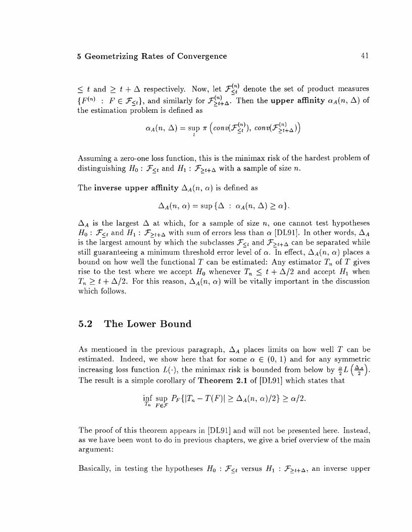
< - t and 2 t + A respectively. Now, let ~ 2 ) denote the set of product measures - {F(") : F E FCt), - and similarly for FE!;:&. - Then the upper affinity a ~ ( n , A) of the estima.tion problem is defined as
Assuming a zero-one loss function, this is the minimax risk of the hardest problem of distinguishing Ho : .F<t - and HI : - with a sample of size n.
The inverse upper affinity AA(n, a) is defined as
AA(n, a) = sup {A : aA(n , A) 2 a ) .
AA is the largest A at which, for a sample of size n , one cannot test hypotheses Ho : FSt and H1 : F2t+A with sum of errors less than cu [DL91]. In other words, AA is the largest amount by which the subcla,sses fit - and F>t+A can be separated while still guara,nteeing a minimum threshold error level of a. I n effect, AA(n, a) places a bound on how well the functional T can be estimated: Any estimator T, of T gives rise to the test where we accept Ho whenever Tn 5 t + A/2 and accept Hl when Tn 2 t + A/2. For this reason, AA(n, a) will be vitally important in the discussion which follows.
5.2 The Lower Bound
As mentioned in the previous paragraph, AA places limits on how well T can be estimated. Indeed, we show here that for some a E (0, 1) and for any symmetric increasing loss function L(-) , the minimax risk is bounded from below by YL (%). The result is a simple corollary of Theorem 2.1 of [DL911 which states that
inf sup PF{ITn - T(F)( > A A ( ~ , ~)/2) 2 ~ / 2 . Tr, F E F
The proof of this theorem a.ppears in [DL911 and will not be presented here. Instead, as we have been wollt to do in previous cha.pters, we give a brief overview of the main argument:
Basica,lly, in testing the hypotheses Ho : F<t - versus HI : . F 2 t + ~ , an inverse upper
5 Geometrizing Rates of Convergence
affinity of AA(n, a) implies that Type I and Type I1 errors2' together sum to a mini- mum risk level of a22, SO that at least one of these error Types must incur a risk of " 2 ' Now, with a test which decides Ho if Tn 5 t + 4 and HI if Tn > t + 4, a Type I or Type II error can occur only if the estimate T, is on the 'wrong' side of the point t + 4; in other words, only if ITn - T(F)I 2 4. Combining these two observations, the probability23 that Tn differs from T(F) by at least 4 is lower bounded by f for the worst case F.
5.3 Attaining the Lower Bound: The Binary Search Esti- mator
In the previous subsection, we established AA(n, 0 ) / 2 as a lower bound on the rate of risk convergence to zero for some fixed a E (0, 1). The proof involved showing that even with tlze best of all possible estimators Tn, hypothesis testing techniques would always yield a worst-case risk proportional to L (v). In this section, we describe an actual estimator Tn which is optimal to within con- sta.nts, in the sense that, under certa,in conditions, it too converges to T(F) act a rate which is a constant multiple of AA(n, a). In this case, though, the actual worst-case risk is pro~ortional to L(KAA(n, a ) ) , where IC may he substantially larger than 4.24 Nevertheless, the fact that AA forms a lower bound together with its (near) attain- ability establishes it as an optimal rate of convergence.
The estima.tor proposed in [DL911 a,ssumes a compact pa,ra,meter space T ( F ) E R = [-d, dl. Consider an estimator constructed from repeated hypothesis tests where each successive test enables us to shrink the search space and to honle in on T(F) in a manner akin to a Binary Search. During each phase we perform a minimax hypothesis test between the lower third and upper third of the current search space, with the middle third adopting the role of 'A' in our previous discussions on hypothesis testing. The new search space is fornled by deleting whichever third - upper or lower - is rejected by the test. Hence, each pha.se of the sea,rch yields a search space the size of the previous one; after a prescribed N phases we are left with an interval a
"False rejection and false acceptance respectively 22Consult definitioil of inverse upper affinity above 23measured according t o the distributioil F mllose parameter we are attempting to estimate 24See Section 5.5 for details.
5 Geomet r i z ing R a t e s of Coilvergence
fraction ($)N of the length of the initial space, whereupon we select the midpoint as our estimate.
Let us refine this idea with a few details: First of all, we endow our 'Binary Search Estimator' TBin with a 'tuning constant' A, which varies with sample size but is fixed for any given n. A, is the length that we wish the search space finally to have after all N tests; if no error occurs during any of the hypothesis tests, then TBin will differ from T(F) by no more than %. The number of successive tests we need perform is then N = N(d, A,), the smallest integer such that d' = (z)N% > d, while the starting search space is [-dl, dl] > SZ and the initial hypothesis test compares Ho : F5-d'/3 against Ho : F>dt/3.
Naturally, the minimax risk associa.ted with TBin is the accumulated risk from all N hypothesis tests. More precisely, using TBin as an estimatorz5,
where a a (n , % (1)') , is the upper affinity of the (N - k) th hypothesis test. Though
this last sum may look unwieldy, if A, is made a constant multiple26 of the inverse upper affinity A A ( n , a ) , Theorelm 2.3 of [DL911 shows that the sum of upper affini- ties can be made arbitrarily sinall provided only that AA exhibits appropriate tail behaviour. Hence, under this condition, TBin is seen to attain the desired rate of convergence, a constant multiple of AA .
5.4 Ensuring Appropriate Tail Behaviour of AA
The reader would he justified in surmising that it may prove difficult to obtain AA(n, a) in closed form, let alone derive properties concerning its tail behaviour. In this section we side-step the former problem, a.nd instead focus on the latter, showing that asymptotic heha.viour of AA may be derived indirectly by wa.y of the modulus of continuity.
The required tail behaviour we would like AA to exhibit is:
251t should be noted that Tsi, incorporates N 'sub-estimators' TnY1, . . . , T n , ~ (one for each suc- cessive hypotl-lesis test), no two of which need be the same.
260nce again, the reader is referred to Section 5.5 for a discussion of the magnitude of this constant.
5 Geometrizing Rates of Convergence 44
For fixed a E (0, I ) , there should exist q > 0 and 0 < A. 5 Al < m such
that
for suitably large n.
If this is indeed the case, then the supporting conditions of Theorem 2.3 of [DL911 are met, and, as discussed in the previous section, Tsi, is seen to achieve the desired rate of convergence. This ra,te is proportional to AA; from Inequality ( 1 2 ) the rate is,
hence, 0 ( 1 2 - ~ / ~ ) .
Now, in genera#l, the validity of Inequality (12) may be difficult to show. However, it is possible to show that if the geometry of T and .F conform to certain criteria, then
( ) - < , 5 ( c p )
where b(6) is the modulus of continuity described in Section 5.1.3. The geometric criteria necessary as well a.s the derivation of the above inequality are discussed in Sections 5.4.1 and 5.4.2. In the mea.nwhile we note that if Inequality ( 1 3 ) can indeed be established, then the problem is simplified dramatically: The establishment of b ( ~ ) as a Holder function is all that is necessary to transform Inequality ( 1 3 ) into a form which satisfies Inequality (12). The rate of convergence is, thus, b ( ~ 2 - ' / ~ ) . See Figure 5.
It would seem at first gla.nce t11a.t we have simply replaced one set of criteria with another. This is indeed the case; however, as we will see in Sections 5.4.1 and 5.4.2, the replacement criteria are fa,r easier to dea.1 with.
5.4.1 The Case of Linear T and Convex .F
In this section, we show that sufficent conditions for Inequality ( 1 3 ) are linearity of the functional T and convexity of the distribution cla.ss F. It can be shown that the lower bound of 1neclua.lity ( 1 3 ) can a1wa.y~ be established; it is the upper bound which needs some work.
5 Geometrizing Rates of Convergence 4 5
We begin by extending the notions of Hellinger Affinity and Hellinger Distance2? to classes of distributions. For two classes of distributions P and Q, define
p ( P , Q) = sup {p(P, Q) : P E P, Q E Q), and
H(P, Q) = iilf {H(P, Q) : P E P , Q E Q}.
Now, for % E F , consider the Hellinger ball BH(c, k) = {F E .F : H ( F , F) 5 6 ) .
By the definition of the modulus of continuity2', {T(F) : F E Bx(c, F)} C [T(B) - b(e), T(P) + b(c)], so that for any t in the parameter space 0, H(F<t, - F>t+acc)) - 2 c. Recalling the identity H2(P, Q) = 2(1 - P(P, Q)), this leads to
Now the crucia.1 observation is that if T is a linear functional and F is a convex class, then F<t - and F>t+a - are both convex, for a.11 t and all A. Hence, F<t - = ~onv( .F<~) - and
F>t+b(e) = c~nv(F>t+b(r)), SO thamt
Now, Le Ca.m 11a.s esta.hlished ([LeCsG], pa.ge 477) that
where P and & are distribution classes a.11~1 ?("I and Q(") are the classes of corre- sponding product measures. Le Can1 has also shown that p(P, Q) 2 T ( P , Q) where r ( P , Q) is the testing affinity29 between distributions P and Q. If we put P = F<t -
aad Q = .F>t+b(c) - and ta.ke suprema over t , Inequality (15) then yields
Finally we substitute Inequality (14) into this last, to yield
a . ( n ( ) 5 1 - - , whence ( ;)"
27See Sections 5.1.1 and 5.1.2 for definitions. 2%ee Section 5.1.3 for definitioil. 29See Section 5.1.4 for definition.
5 Geometrizing Rates of Convergeilce
A simple application of the inequality (1 - a'/") 5 F, which appears as Lemma 3.3 in [DL91], produces the upper bound of Inequality (13). As mentioned previ- ously, once Inequality (13) has been validated, establishment of the modulus as a Holder function suffices to guarantee that TBin attains the desired convergence rate of b (n-'/2).
Section 6 contain an elaborate example of a case where AA is linked to the modulus via linea,rity of T and convexity of 3.
5.4.2 The General Case
In the previous section, we employed linearity of T and convexity of 3 to establish 1nequa.lity (12). Though t,hese are suJJicien.t conditions, we demonstrate here that they are not ~zecessa~.y. Indeed, the link between AA and the ~ilodulus follows from an underlying geometric property, of which linearity of T and convexity of 3 constitute just one of inany possible manifestations.
The essential geometric property is that the hardest two-point subproblem of testing T ( F ) 5 t versus T ( F ) >. t+A should be roughly as difficult, from a minimax risk point of view, a,s the full composite hypothesis-testing problem (i.e. testing Ho : conu(F$')
versus HI : c o n v ( ~ g ! ; : ~ ) - for sample size n).
Define the two-point upper affinity cu2(n, A) and the two-point testing bound A2(1z, a) as
Note the oillission of convexification in colnparison with the definitions of a~ and AA. Now, some identities concerning Hellinger Affinities and Hellinger Distances combined with a little algebraic n~a,slipulatioil lead directly to an inequality identical to that of (12), but involving A2 in pla,ce of AA.30 The details may be found in [DL91]. It now becomes apparent that this new inequality leads immediately to Inequality (12) provided only that AA is roughly equal to A,. Consult [DL911 for more precise criteria.
301ndeed this new inequality, combined wit.11 the fact tha t Az(n, a ) 5 AA(n, a) since a2 5 a ~ , accounts for the lower bound of Inequality (12).
5 Geonletrizing Rates of Convergence
Yet, even this last criterion concerning the hardest two-point subproblem may be discarded, as long as the connection between AA and the modulus can still be made. Indeed, In Exanlple 5.2 of [DL91], Donoho&Liu show that a suitable relationship between A2 and AA is elusive and we are forced to resort to other methods to find a link between AA and the modulus of continuity.
Nevertheless, no matter how the connection with the modulus is made, b ( ~ ) still needs t o be a Holder function in order to establish Inequality (12) and hence ensure that TBin achieves the desired convergence rate of b (n-'I2).
5.5 Link with Estimation Theory
In Section 5.2 we identified AA(7a, a ) as a lower bound, to within constants, on the rate of convergence of T,(X,,) to T ( F ) . More specifally, we reiterated Theoreill 2.1 of [DL91], which states that
inf sup PF{(T , - T(F) I > A,(n, a ) / 2 } > a / 2 . Tn F E F
We then went on to show tha.t for some constant Ir', Ir'AA(n, a ) is an attainable rate of convergence, whence AA(n, a ) emerges as the optimal rate of convergence to within constaizt.~.
In this section, we a,na,lyze the ca,veat "to within constants" from a Decision-Theoretic standpoint. We show that this description, though a.ccurate, may be misleading in the sense that the constants involved will not, as is often the case, be swallowed up during our passage to the infinite. h/Ioreover, tlie constants, though finite, a,re unbounded: classes of distributions can be foullcl for which the constants are arbitrarily large and, correspondingly, the ra.te of uniform convergence arbitrarily reduced.
Consider the following problem of minilnax loca,tion parameter estimation [ZhI84]: Let F be soille distribution with an even, unimoda.1 density function. Define the distribution class F = I F ( - - 0 ) : 0 E 0 = [-d, dl}. The functional we are attempting to estimate is T(Fo E F) = 0 . Let A denote the action space of the s t a t i s t i c i a s ~ ~ ~ , and let L(T,(X,). 0 ) denote the zero-one loss function defined on A @ 0 :
311n this case, A = [-d, 4.
5 Geometrizing Rates of Coilvergeilce
where e > 0 is given.
In [ZM84] it is shown that for the case d = 2e, the minimax risk is cr = F(-e) , while at the other extreme, for d t m e , cr t 2F(-e). In other words,
If we fix the risk level at a and compare the relative sizes of the confidence intervals e;? and e, in the two ca.ses, we see that, thanks to the evenness of F,
so that
em - (I - ) F-I (q) -- - - - e:! F 1 - a ) F-I (a) '
We now make the connection with Aa4(n., a ) . Note that for any t E R, conv(FSt) =
F<, - and ~ o n v ( F > ~ + ~ ) - = F2t+A. Hence, owing to the unimoda.lity and evenness of F , the upper affinity of the estilnation probleln is, for 72 = 1,
Thus, the inverse upper affinity for n = 1 may be derived:
Now, in both the fixed-size confidence procedure and the hypothesis-testing settings, loss can be incurred only if the estimate differs from the true value of the location parameter by a t least e or A A ( l , a ) /2 . Hence, A A ( l , a ) / 2 can be identified with e in Equa.tion (16) a.bove. But which e should we use, e2 or e,?
If we set A A ( l , a ) / 2 = ea for some a, the lower bound in Theorel11 2.1 of [DL911 is seen to correspond esa.ctly with Equa.tioll (16) a,bove in the d = 2e case, with
5 Geolnetrizing Rates of Convergence
minimax risk of ;. However, for the d = m e case, the minimax risk then becomes twice the lower bound of Theorenl 2.1.
In order to preserve the risk level at ; and hence accommodate all scenarios, we resort to setting A A ( l , a ) /2 = e,. Thus we see that the optimal rate of conver- gence of estimator to parameter, AA( l , a), must be slowed b y a factor of e,/e2 =
F - I (;) I F - l ( a ) .
This reduction in rate of convergence would not be as noteworthy if it were not for the fact that relatively simple classes of distributions may be found which satisfy the unimodality a,nd e\~enness criteria a,nd for which the factor F-' (q) I F - ' ( a ) can be ma,de arbitrarily 1a.rge.
Example: The Contaminated Norlllal distribution Consider a Contaminated Norma,l distribution, F,,, = (1 - c)N(O, 1) + eN(0, v ) for some 0 5 e 5 1 and v E [I, Go) .
Figure 7 shows a plot of F;,' (q) / F $ ( a ) for v = 100, s = & and 0 < a < 0.25. For comparison, the curves for Norma,l, Cauchy, and Laplacian F are also show11.
Let us now focus our attention on the Contaminated Normal distribution: Figure 8 illustrates F;: (f) /F$(a) for various values of variance a of the contaminant, with
e held constant at &. The shape of the surface bears out what many evaluations
of F;: (:) 1Fc.a) for r = h, a = 0.05 and v ra,nging from 1 through 10' seem
to suggest: that the inaximun~ value of the curve increases as CJ;; where C FZ
0.2355. 111 other words, tlhe fa,ct,or by which the ra.te of coilvergence is slowed seems to be proportiona.1 t,o the sta.ndard deviation of the contaminant, and is therefore unbounded.
As a fina.1 note, it should be empllasized that the deinonstration of the possibility of unbounded constants is intended merely to warn the unwa,ry and to discourage the blind application of the results; it is certainly not meant to detract from a.n otherwise very general and very powerful result.
5 Geometrizing Rates of Convergence
Figure 7: Plot of F-I (q) / F " ( c Y ) as a function of 0 5 CY 5 0.25 for F Normal, Cauchy, Laplacian and Contaminated Normal ( f t N ( 0 , 1) + $ N ( o , 100)).
Figure 8: Plot of the factor e,/e2 = /F;:(cY) as a function of 0 5 a 5 0.2 and 1 5 v 5 500 ontaminated Normal distribution, where 6 is held constant at A.
6 Rate of Convergence over a VC Class
In order to gain insight into the manner in which the results of [DL911 may be applied, consider a relatively simple setting: Let us derive a lower bound on the rate of uniform convergence of relative frequency to probability over a class of events A c 13 with respect to the probability space (X, 13, P).
Section 3 summarized the result of [VC71] that a sufficient condition for such con- vergence to be uniform over A is merely that A be of polynomial discrimination with respect to the whole space X. We therefore limit our analysis to such a class of events, and derive rates of convergence for estimators of P(A) , using methods outlined in [DL911 and described in Section 5 . 3"
We begin by transforming the problem into a form to which the results of [DL911 are applicable. We need to find a, suitable distribution class .F and functional T : F t 3.
Let dA : X + {0, 1) denote the indicator function for A E A.33, SO that we can define the stochastic process D = {eA : A E A). Let F denote the correspondiilg class of distributions such that FA E F is the CDF corresponding to the random variable O A . Further, let T be the (linear) functional which returns the expected value of its argument F E F. Hence, for any FA E F, T(FA) = P(A). By establishing a uniform rate of convergence of an esti~nate T,,(X,)34 to the value of the functional T(FA) of an unknown distribution FA E F we simultaneously establish a rate on the uniform convergence of a.ny estimate (including relative frequency) to probability over the class of events A.3"
Having defined F and T, we proceed to derive an expression for the inverse up- per affinity aA(12, a ) for some confidence level a. If AA(n, a ) can then be shown to exhibit appropriate tail behavior, our quest will be accomplished: AA(n, a ) will
321n the interests of consistency, we maintail1 tlle use of the symbol 'A' t o represent an arbitrary member of A , despite the unfortunate clash with the subscripts used in the symbolic representations of upper affinity CYA and inverse upper affinity A A .
33We assume throughout that each event A E A is measureable. 34where X, is a vector of n i.i.d. FA sample points 35Actually, since distinct sets of equal probability have indistinguishable images in 3, much of the
structure of tlle class A rnay be lost in the transformation to F. I t is for this reason that we still insist that A be of polynomial discrimination to guarantee uniformity over A; the uniformity result established using the results of [DL911 makes a stat.ement only about the distribution class 3, and caiinot be extrapolated back to the generating class of sets A. Hence, zf the conditions of [VC71] are satisfied by A , then convergeilce will occur at best a t the rate prescribed by [DL91].
6 Rate of Coilvergeilce over a VC Class
represent the optimal rate of convergence, to within constants.
In Section 6.1 we derive an expression for AA(n, a ) using various graphical and empir- ical techniques. For an arbitrary generating class of sets A, we derive testing affinities and the upper affinity oA(n, A) en route to the inverse upper affinity AA,(n, a ) which is seen to display n-'I2 tail behavior. Then, in Section 6.2, we show how the geom- etry of the problem, in the form of the modulus of continuity, may be exploited to short-cut the derivation.
6.1 Graphical and Empirical Approach
Recall the definition of the upper affinity
aA(n, A) = sup a ( c o a v ( F k ) ) , conu(F'gyA)) t - -
where F<t a.ncl F>t+a denote the subsets of F' where T takes values 5 t and > t + A respectively, denotes the set of product measures Fin) , F E F , and a ( P , Q ) represents the testing affinity between the classes P and Q. Recall also the identity
Now, for the current exa,mple, a.n a,rbitra.ry member FA : 92 -+ [ O , 11 of 3 ha,s the profile
for x E (-w, 0 ) F A ( z ) = - P ( A ) for x E [0, 1 )
for x E [ I , m)
so that T ( F A ) a.lso corresponcls to fA(l), where , f A is the P M F of FA. Let FA have the dual nota,tion Ft, where t = T ( F a ) = P(A) . Then the product measure F:;(") is seen to have a PMF f jn) defined on 'Rn as:
( t ) ( x i x') (1 - t ) ( n - x f "') for ( Z 1 , 2 2 , . . . , Z,) E {O, f j n ) ( x l , xi, . . . , x n ) =
l o for (x', Z 2 , . . . , x n ) # (0, 1In.
Hence, for 0 < A 5 and 0 5 t 5 1 - A,
6 Rate of Convergence over a VC Class 53
It is already clear that a purely theoretical analysis will soon become overwhelmingly complicated. We therefore resort to numerical and graphical tools for assistance.
Figure 9 shows a plot of a (Fin), ~::;!"k) as a function of t and A, with n = 6. Similar plots for various values of n yield surfaces which all share the following algebraically verifiable properties:
1. For fixed t , a (Fin), F$L) is monotone decreasing in A
2. For fixed A, s (Fin) , F$;:"k) exhibits (n - 1) cusps36, as shown in Figure 10.
Furthermore, a (F:"), F:T~) is maximized at the cusp nearest the hyperplane 1-A t = -
2 .
3. The surfaces a,re sym~netrica,l about the hyperplane t = 9 over the region o < n 1 1 , 0 1 t ~ 1 - n .
From property (1) we deduce that
("1 In words, the most error-prone two-point testing problem betweell F<t and .'F>t+a OC-
curs for elements which reside on the very 'edges' of the classes, and-whose functional values a.re, hence, as close to each other ass possible. Moreover, a rea.ter testing affin- ("7 ity cannot he generated even if the converified classes conv(F<, - ) and c o n v ( ~ c \ ~ ) -
are tested i the stea,d of .F$) and This last is a consequence of the following - two facts:
The functions t k ( l - L ) " - ~ , k = 1, 2, . . . , 12 are unimodal over 0 5 t 5 1;
For the calculation of a (F:~), ~$ : ; " k ) , we select the smaller of t k ( l - t)"-' and
( t + A)"1 - t - A)n-k for all b = 1, 2, . . . , 12.
3 6 ~ t call be shown that for fixed A , t,he cusps occur at, t sa.t,isfying
6 Rate of Convergence over a VC Class
as a function of 0 5 t 5 0.5 and 0.04 j
Figure 10: T ( F ) as a function of 0 5 t 5 0.6 for fixed A = 0.05 and 12 = S, 10. Both functions are lnaxilllized at t = I - n =
2 0.475.
6 Rate of Convergence over a V C Class
For even n, properties (2) and (3) imply that the cusp which maximizes T (Fjn', F'/:i) I - A occurs a t t = T .
Combining all these observations, we deduce
c ~ ~ ( I I , A) = sup W (conv(.F$)), conv(~$!;:~)) t -
= sup T (Fjn), F$,!"k) t
Exploiting symmetry, we conclude that, for even n,
A plot of a ( n , A) is shown in Figure 11.
R.ecal1 now the definition of the inverse upper affinity
A,(n, a ) = sup {A : a A ( n , A) > a ) .
For a fixed confidence level a, the graph of AA(iz, a ) versus 12 corresponds to the contour line a.t height a on the surface of aA(n, A). Hence, the contour plot of Figure 11 a.ctually serves a.lso a.s a plot of AA(tz, a) versus 12 for a = 0.1, 0.2, . . . , 0.9. Each curve is seen to follow for some value of c, whence we conclude that An(n, a) displays the required tail beha.viour delineated in Inequality (12) of Section 5.4. The
conditions of T h e o r e m 2.3 of [DL911 are met, and AA(n, a) = 0 (n-'I2) emerges as the optimal rate of convergence of an estimator to T(FA) = P ( A ) , A E A.
It should be emphasized that this is only an empirical result, abounding in empirical observation ant1 heuristic deduction and lacking somewhat in rigour. It would seem that without some complicated algebra, we have reached an impasse in our quest for a precise expression for the optima.1 rate of convergence.
6 Rate of Convergence over a VC Class
Figure 11: 3-Dimensional Plot and Contour Plot of a A ( n , A) for 0 < n < 150 and 0.02 - < A - < 0.2.
6.2 The Modulus to the Rescue
We showed in Section 5.4.1 that the problem of deriving optimal rates of convergence is greatly simplified provided
1. The functional T is linear,
2. The class F is convex, and
3. The lnodulus of continuity of T with respect to F, b ( ~ ) , is a Holder func.tion of exponent q.
Indeed, if the geometry of F and T satisfy these three criteria, we can immediately conclude tha t the optimal rate of convergence is b (n-'I2) = O (n-91').
For the current setup, the functional T returns the expected value of its argument F E F, and is, thus, linear. Though A does not necessarily generate a convex F, we can continue the analysis using conv (7 ) as the distribution class. Of course, the price to be paid is that the rates will no longer necessarily be optimal since we are
6 Rate of Convergence over a VC Class
dealing with a superset of the original class37. Nevertheless, there are many interesting examples of VC classes A for which F is itself convex3' and nothing is lost. We assume henceforth that F is convex.
The only remaining criterion concerns the modulus of continuity b(e), to which we now turn our attention.
Recall the definition of the modulus of continuity of T over F
Here H ( F l , Fo) is the Hellinger Dista.nce between two probability mea.sures Fl and Fo in F and is defined as
where fl and f o are the PMF's of Fl and Fo respectively.
In our case, the PMF ft is defined as
1 - t f o r x = O for x = 1 for x E SIZ, x $ (0, 1)
Hence, the Hellinger distance between two arbitrary members F, and Fp of F is
Figure 12 shows a plot of H(F,, Fp) as a function of a and P. Contour lines represent the skins of Hellinger balls, so that from the figure we see that for any Hellinger ball of radius 6 , the quantity la - ,Bl is maxi~nized on the skin of the ball at a = 1 - P. Substituting into Equation (17) yields, for any 0 5 c < 1,
1-a-fi)2+(fi-,/izq2 H(F,, &,I = 6 = /I" 2
370n the other hand, if we could find a convex subset of 3, the rate of convergence for the subset would form a lower bound on the optimal rate for F. However, this lower bound inight no longer be attainable.
3"Consider, for inst.ance, the class A of intervals of 92.
6 Rate of Convergence over a VC Class
Figure 12: 3-Dimensional Plot and Contour Plot of H(F,, FD) as a functioil of a and p.
Hence, 2 = 1 - 24a(l - a ) 2
so that (y) = a - n 2
1 7 Jl - (1 - ~ 2 ) ~ whence a =
2
From here we can derive the modulus of continuity: For any 0 < r 5 1:
A Taylor Series expansion yields b(r) = f i e - $r3 - O(r5), so that for small 6, b(r) is seen to be Hlilderian of exponent 1. We conclude that the rate of conver-
6 Rate of Coilvergeilce over a VC Class
gence optimal for all possible estimators of T ( F A ) , including relative frequency, is b (n-'I2) = O (7%-'I2), and that this rate is, in fact, attainable.
Finally, the astute reader may be perturbed by a possible incongruity between of the above result and that of Inequality ( 5 ) . Indeed, fixing Fn as the relative frequency estimator, the methods of [DL911 have lead to the lower bound
On the other hand, if the genera,ting class of events A is of polynomial discrimina,tion, and we denote the order of the majorizing polynomial by d 39, then the approach of [VC71] leads to the upper bound
for n > d/2.
With respect to the probability space (9, B , P), define, for each F E 3 the 'bad- set' BF(6) = {$ € 9 : jFn - T(F)I > 6). The lower bound of [DL911 then limits the rate of convergence to zero of the probability of the largest4' bad-set supFE3 f' ((BF(AA/2)), while the upper bound furnished by [VC71] guarantees a rate of 4 (2n + l)d e-12n/8 for the convergence to zero of P {sup,,, ifn - T ( F ) I 2 6 ) =
P {UFEF BF(~ ) ) .
Hence, if we equate E = AA(??, a ) / f l , elementary set theory a,llows us to rela.te the two bounds:
> sup P Bf (c ) = sup P B F ( A A / ~ ) ) FEF ( F E 3 (
It would seem that the expollentially decrea,sing upper bound may quickly dinlinish to less tha.11 the lower bound! The resolution of this a.ppa.rent contradiction, however,
3gd is called the VC-dimension of A. 4 0 ~ i t h respect to measure P
6 Rate of Convergence over a V C Class
lies in the fact that 6 , now equated with AA(n, a ) , is no longer a constant, but is instead monotonically decreasing in n. Indeed, the rate of decrease of e is sufficient to compensate for the apparent exponential decay of the upper bound: In the above exa.mple we showed that AA(n, a) is proportional to b(n-li2) where b(S) is asymptot- ically linear in 6. Hence, putting E = Cn-lI2 for some constant C , the upper bound is seen to degenera.te into an increa.sing function:
The integrity of the results is preserved.
6.3 Extension to Manageable Classes of Functions
As a final note, we mention that a similar application of the results of [DL911 to a manageable class of functions = {gA : X E A ) allows us to derive a lower bound on the rate of uniform convergence to zero of the empirical process41 operating over this class with respect to the probability space (%, B, P) ".
As in the above example, we begin by caating the problem into a, mold to which the results of [DL911 are applicable. Our first task is to define a suitable class F of distributions on the measureable space (8, 0) and to find a mapping R : G --t F. Furthermore, if a functional T : F t % can be found such that for all g E G, T(R(g)) = P g , then establishing an optimal rate for all estimators Tn : sfEn + % to converge to T uniformly over F is tantamount to establishing a lower bound on the rate of convergence to Ep of a speci@c estimator such as Bp,, the expectation with respect to the empirical measure" PT,. A scaling by a fa,ctor i1 /2 then establishes an analogous bouncl on the ra,te of convergence to zero of the empirical process.
An intuitive choice for the mapping R and the f~~nctional T is to treat g~ as a random ~ a . r i a b l e ~ ~ on (3, B , P), have R(gA) = FA be the distribution of this random variable, and let T (R(gx)) be the expected value of this distribution FA. Regardless of P, the condition T(R(g)) = P g is then satisfied for all g E G , provided P g exists.
41See Sect>ion 4 for definition. 42Where B denotes the Bore1 field on sR and P is some probability measure of finite variance. This
last condition is needed in order for the Cendral Limit Theorem t.o be applicable - see Sect,ion 2 of [Po189].
43See Section 4 for definition. 44We assume here that gx is measureable for all X E A.
6 R a t e o f C o n v e r g e n c e o v e r a VC Class
From here, an expression may be derived for the rate of convergence by methods inspired by [DL91]. In particular, we once again invoke one of the main results of [DL91]:
If T is linear, F is convex, and the modulus o f continuity o f T with respect t o F, b(e) , is a Holder function o f exponent q , then the optimal rate of
convergence is b (n-'I2) = U (n-qI2).
Since T is an expectation, it is linear. In general, however, .F is n o t necessarily convex. The simplest remedy is to derive an optimal rate of convergence for the class coizv(.F) rather than for F. Of course, the price of the silllplification is that b(n- ' I2) is demoted from its position as optimal rate to a hurrlble status of upper bound for the minimax estimator TBin described in Section 5.3. However, provided the losses incurred by convexification do not exceed the gains furnished by the use of an optimal estimator instead of lEp,,, the validity of the main claim - that b ( 1 2 - l / ~ ) forms a lower bound on the empirical process rate of convergence - is not jeopardized4'.
Hence, all that remains to be done is to derive an expression for the modulus of continuity b ( ~ ) of T with respect to conu(.F). Provided convexification losses are not excessive, verification that b ( ~ ) is Holderian of exponent q is sufficient to establish b ( 1 2 - ' / ~ ) = U ( i x - q I 2 ) a,s the lower bound on the rate of uniform convergence to zero of the empirical process operating over S.
45Evei~ in the case where coiivesificatioil losses outstrip the gains provided by an optinzalestimator, some significaiice can still be gleaned froin the results: b(n-'1') then forms an upper bound on the empirical process rate of convergence, guaranteeing a certain rate. Moreover, it may yet be possible to establish b(7z-'/') as a lower boulid as well, using methods fro111 [DL911 which do not rely on the convexity of 3 (See Section 5.4.2 for elaboration). Hence, even greater import is imparted to the rate b(n-'l": Since it forills an upper a n d lower bound on the empirical process rate, a.symptotic equality of the two rates inay be inferred.
Conclusion
It was the ambition of this survey not only to give conspectuses of the main threads of each of the three papers [VC71], [Pol891 and [DL91], but also to expose their intricate intertwinement and interdependence.
The first paper, [VC71], addresses the problem of establishing criteria subject to which one may conclude that the relative frecluencies of events converge t o their probabilities uniformly over a class A c B with respect to the probability space ( Q , B, P). The results are twofold:
1. A sufficient condition for unifor~n convergence is that the class of events be of polynomial discriminatio~a. No coilstraints need be imposed on the distributioil P.
2. A sufficient and necessary condition for uniform convergence is the asymptotic approach to zero of the ratio of entropy HA(E) to sample size I . Since the entropy of a class of events A is defined as the expected value of the index of A, the satisfaction of t,his condition depends upon the distribution P.
The results of [VC71] continue to be pertinent to, and have impact upon, areas such as Neural Network Theory and Lea.rning Theory. Though stronger results have emerged since its publication, the paper retains its pre-eminance, if not for its continuing general applicability then for the sheer elegaace of its derivations.
The second pa,per, [PolSS], sees the extension of the ideas of [VC71] to a class of fu~zctio~zs 6. The maill concern is the establishn~ent of criteria for which convergence of the empirical nleall P, g to the actual mean P g may be guaranteed uniformly over G. The climax of [Pol891 is ba,sically that the desired uniformity is attained provided G is a inallageable class, along with a few subsidiary conditions. The link with [VC71] is strengthened by the ra.ther remarkable result that if {subyraph(g) : g E G) is of polynomial discrimina.tio11, t,llen Cj is, in fact, a manageable class of f~ulctions.
Perhaps more than in the actual results, however, the significance of [Po1891 lies in its exposition of a very powerful technique for the analysis of the entire family of problems involving averages of functions of independent observations, of which the problem scrutinized here - that of finding criteria under which these averages converge uniformly to the expected values of the functions - is a member.
Any treatment of convergence concepts would be incomplete without a discussion of rates of convergence. The theme of [DL911 revolves around a bound on the rate of convergence of an estimate Tn(X,)46 to the value of a functional T(F) of an unknown distribution F E F uniformly over a class of distributions F. The main result is that for estimating a linear functional over a convex distribution class F , the geometry of the problem, expressed in terms of the modulus of continuity b(c), determines the optimal rate of convergence. Moreover, if b(t) is a Hijlder function of exponent q, the optimal rate is b (n-'I2) = @ (n-qI2) and is, in fact, attainable. As an encore, it is further shown that the prerequisites of linearity and convexity may be discarded, provided that the essence of the geometry is preserved: A new criterion is that the hardest two-point subproblem of testing T ( F ) 5 t versus T ( F ) > t + A should be roughly as difficult, from a minimax risk point of view, as the full composite hypothesis-testing problem.
As mentioned in the Introduction and demonstrated in the elaborate example of Section 6, a little reflection shows the results of [DL911 to be directly applicable to the convergence problems a.nalyzed in [VC71] and [Po189]. Indeed, given a class of functions G", each function g E G may be construed as a random variable with respect to the probability space (3, B, P). Let .F be the class of marginal distributions of the resultant stochastic process, a,nd choose the (linear) functional T(F), F E .F to be the expected value of F, i.e. T ( F ) = P g where F E F is the distribution of the randoln va.riable g E G. Esta,l)lisliing the nlodulus of continuity of T over co7zv(F) as a HKlder function of exponent p pla,ces a lower bound of b (IL-'/~) = O (11-q/~) 011 the rate of u~lifor~n convergence to T ( F ) of any estimate Tn(X,), including the empirical expectation P, g .
Of course, the results of [DL911 extend fa.r beyond these rather confined cases. Indeed, the power and generality of the results is matched only by the scope of their appli- ability: Nonpa,ra.met,ric di~t~ribution cla.sses succumb t,o invest,iga.tion a.s tra.ct#a,bly as parametric classes, and the latitude afforded in the choice of functional T is virtually unconstrained. For these reasons, the results of [DL911 may very well assume a piv- otal role in future research within the field of stochastic processes and their rates of convergence.
46wl~ere X , is a vect,or of n i.i.d. F sample points 476 could be a, cla.ss of iildicat,or funct,ions if classes of evei~t~s are iilvolved a.s in [VC71].
Papers Surveyed
[VC71] Vapnik & Chervonenkis: (1971) On the Uniform Convergence of Relative Frequencies of Events t o their Probabilities. Theory of Probability and its Applications, 1971, Vol. 16, NO. 2, 264-280.
[Far661 Farrel l , R. H.: (1966) On the Lack of a Uniformly Consistent Sequence of Estimators of a Density F~lnction in Certain C u e s ,
[Far721 Far re l l , R. H.: (1972) On the Best Obtainable Asymptotic Rates of Convergence in Estimation of a Density Functioil at a Point. The Annals of Af(~thematica1 Statistics, 1972, Vol. 43, No. 1, 170-180.
[GD86] G r a y & Davisson: (1986) Random Processes: A Mathematical Approach for Engineers, Prentice-Hall.
[I<F70] Koln logorov & Fornin: (1970) Jirtroductory Real Arznlysis, Dover
[LY90] L e C a m & Yang : (1990) Asymptotics in Statistics: Some Basic Concepts, Springer-Verlag.
[LeCSG] L e Cam, L.: (1986) Asymptotic ilfethods in Statistical Decision Theory, Springer-Verlag.
[Ma1881 Mal l e r , R. A.: (1988) Asymptotic Norma.lity of Trimmed Means in Higher Dimensions. Tlze A7zizals of PI-obability, 19S8, Vol. 16, No. 4, 1608-1622.
[Mintz] Mintz, M. A Review of some ideas in Afens~~re Theory and Probability Theory Lecture Notes, pp 51-500.
[Pol841 P o l l a r d , D.: (1984) Convergence of Stochastic Processes, Springer-Verlag.
[RomSS] R o m a n o , J. P.: (1988) On Weak Con\rergence a.nd Optirna,lity of Kernel Density Estimates of the Mode. Tlze Anlzals of Statistics, 1988, Vol. 16, No. 2, 629-647.
[SYSl] Sacks & Ylvisaker : (1981) Asymptotically O p t i n l ~ l ~ l Kernels for Density Estinlation a t a Point. The Annals of Statistics, 1981, Vol. 9, No. 2, 334-346.
7 References
[Sc,h50] Schlafli, L.: (1950) Gesammelte mathematisclze Ablzandlungen, I, Basel, 1950.
[Wen621 Wendel, J. G.: (1962) A Problem in Geometric Probability. Math. Scand., 1962, Vol. 11, 109-111.
[YatS5] Yatracos, Y. G.: (1985) Rates of Convergeilce of Minimuin Distance Estimators and I~olmogorov's Entropy. The Aiz~zals of Statistics, 1985, Vol. 13, No. 2, 768-774.
[ZMS4] Zeytii~oglu & Mintz: (1984) Optimal Fised Size Confidence Procedures for a Restricted Pa,rameter S p c e . Tlze A~z~znls of Stnii.f;tics, 1984, Vol. 12, No. 3, 945-957.