Convergence Properties of the Batch Means Method for Simulation Output Analysis Natalie M. Steiger • James R. Wilson Maine Business School, University of Maine, Orono, Maine 04469-5782, USA Department of Industrial Engineering, North Carolina State University, Raleigh, North Carolina 27695-7906, USA [email protected]• [email protected]We examine key convergence properties of the steady-state simulation analysis method of nonover- lapping batch means (NOBM) when it is applied to a stationary, phi-mixing process. For an increasing batch size and a fixed batch count, we show that the standardized vector of batch means converges in distribution to a vector of independent standard normal variates—a well-known re- sult underlying the NOBM method for which there appears to be no direct, readily accessible justification. To characterize the asymptotic behavior of the classical NOBM confidence interval for the mean response, we formulate certain moment conditions on the components (numerator and denominator) of the associated Student’s t-ratio that are necessary to ensure the validity of the confidence interval. For six selected stochastic systems, we summarize an extensive numerical analysis of the convergence to steady-state limits of these moment conditions; and for two systems we present a simulation-based analysis exemplifying the corresponding convergence in distribution of the components of the NOBM t-ratio. These results suggest that in many simulation output processes, approximate joint normality of the batch means is achieved at a substantially smaller batch size than is required to achieve approximate independence; and an improved batch means method should exploit this property whenever possible. (Simulation; Statistical Analysis; Method of Batch Means ) 1. Introduction In discrete-event simulation, we are often interested in estimating the steady-state mean µ X of a stochastic output process {X i : i ≥ 1} generated by a single, though long, simulation run. Assuming the target process is stationary and given a time series of length n from this process, we see that a natural estimator of µ X is the sample mean X (n)= 1 n n i=1 X i . We also require some indication of this estimator’s precision; and typically a confidence interval (CI) for µ X is constructed with a prespecified coverage probability 1 − α, where 0 <α< 1. We seek to construct a CI for µ X that satisfies two criteria: (a) it is narrow enough to be informative, and (b) its actual probability of covering the point µ X is close to the nominal level 1 − α.
Transcript
Convergence Properties of the Batch Means Methodfor Simulation Output Analysis
Natalie M. Steiger • James R. Wilson
Maine Business School, University of Maine, Orono, Maine 04469-5782, USA
Department of Industrial Engineering, North Carolina State University, Raleigh, North Carolina27695-7906, USA
We examine key convergence properties of the steady-state simulation analysis method of nonover-lapping batch means (NOBM) when it is applied to a stationary, phi-mixing process. For anincreasing batch size and a fixed batch count, we show that the standardized vector of batch meansconverges in distribution to a vector of independent standard normal variates—a well-known re-sult underlying the NOBM method for which there appears to be no direct, readily accessiblejustification. To characterize the asymptotic behavior of the classical NOBM confidence intervalfor the mean response, we formulate certain moment conditions on the components (numeratorand denominator) of the associated Student’s t-ratio that are necessary to ensure the validity ofthe confidence interval. For six selected stochastic systems, we summarize an extensive numericalanalysis of the convergence to steady-state limits of these moment conditions; and for two systemswe present a simulation-based analysis exemplifying the corresponding convergence in distributionof the components of the NOBM t-ratio. These results suggest that in many simulation outputprocesses, approximate joint normality of the batch means is achieved at a substantially smallerbatch size than is required to achieve approximate independence; and an improved batch meansmethod should exploit this property whenever possible.(Simulation; Statistical Analysis; Method of Batch Means)
1. Introduction
In discrete-event simulation, we are often interested in estimating the steady-state mean µX of astochastic output process {Xi : i ≥ 1} generated by a single, though long, simulation run. Assumingthe target process is stationary and given a time series of length n from this process, we see that anatural estimator of µX is the sample mean
X(n) =1n
n∑i=1
Xi.
We also require some indication of this estimator’s precision; and typically a confidence interval(CI) for µX is constructed with a prespecified coverage probability 1 − α, where 0 < α < 1. Weseek to construct a CI for µX that satisfies two criteria: (a) it is narrow enough to be informative,and (b) its actual probability of covering the point µX is close to the nominal level 1 − α.
The usual method of CI construction from classical statistics, which assumes independent andidentically distributed (i.i.d.) normal random variables, is not directly applicable to analysis ofa steady-state simulation model since successive observations of a simulation-generated outputprocess typically fail to be independent, identically distributed, and normal. Among the varioussteady-state simulation analysis techniques that have been developed for constructing CIs basedon dependent output processes, the method of nonoverlapping batch means (NOBM) is one of themost widely used in practice (Law and Kelton 2000).
In the NOBM method, the sequence of simulation-generated outputs {Xi : i = 1, . . . , n} isdivided into k adjacent nonoverlapping batches, each of size m. For simplicity, we assume that nis a multiple of m so that n = km; thus when k is fixed and m → ∞, we have n → ∞. The samplemean, Yj(m), for the jth batch is
Yj (m) =1m
mj∑i=m(j−1)+1
Xi for j = 1, . . . , k.
The grand mean of the individual batch means,
Y = Y (m, k) =1k
k∑j=1
Yj(m) , (1)
is the usual point estimator for µX (note that Y (m, k) = X(n)); moreover the desired NOBMconfidence-interval estimator of µX is generally centered on (1).
The NOBM method seeks to make each batch a “repetition” of the experiment on the targetoutput process. To achieve this, classical NOBM procedures attempt to determine a sufficientlylarge batch size, m, and the corresponding number of batches, k, to ensure that the resulting batchmeans are approximately i.i.d. normal random variables. With such a setup, it is hoped that theclassical confidence-interval estimation procedure based on the associated Student’s t-ratio will yielda confidence interval for µX with approximately the desired coverage probability. In this paper, weexamine the asymptotic behavior (as m → ∞ with k fixed) not only of the vector of batch meansbut also of the numerator and denominator of the NOBM t-ratio upon which the classical CI isbased.
The rest of this paper is organized as follows. In Section 2 we review the basic assumptionsand distribution theory constituting the background for the NOBM method; and we establish acentral limit theorem for the standardized vector of batch means that is essential to the validityof classical NOBM confidence intervals but is not well documented in the simulation literature.In Section 3, we formulate certain moment conditions on the numerator and denominator of theNOBM t-ratio that are necessary conditions for the distributional requirements detailed in Section2. Section 4 displays the effects of increasing batch size with respect to these limiting conditionsin six selected stochastic processes; and for two of these processes, Section 5 summarizes extensivesimulation results showing the corresponding convergence in distribution for the numerator anddenominator of the NOBM t-ratio with increasing batch size. In Section 6 we summarize the main
2
findings of this work, and we reference follow-up research in which we formulate and evaluate animproved batch means procedure based on the present findings.
2. Background
We assume the target output process {Xi} is stationary (in the strict sense) so that the joint distri-bution of the Xi’s is insensitive to time shifts. We also assume the process is weakly dependent—thatis, Xi’s widely separated from each other in the sequence are almost independent (in the sense ofφ-mixing ; see Billingsley 1968) so that the lag-q covariance
satisfies γ(q) → 0 as |q| → ∞. These weakly dependent processes typically obey a Central LimitTheorem (CLT) of the form
√n[X(n) − µX
] D−→n→∞ N
(0, σ2) , (2)
where
σ2 ≡ limn→∞nVar
[X (n)
]=
∞∑i=−∞
γ(i) = γ(0) + 2∞∑i=1
γ(i)
is the steady-state variance constant (SSVC) (as distinguished from the process variance σ2X ≡
Var[Xi] = γ(0)). A sufficient condition for the SSVC to exist is that∑∞i=−∞ |γ(i) | < ∞ (Anderson
1971). General conditions under which (2) holds are given, for example, in Theorem 20.1 ofBillingsley (1968).
Although some output analysis methods attempt to estimate the steady-state variance constantσ2 in constructing a CI for µX , the classical NOBM method (with a fixed number of batches) doesnot. A key assumption of the NOBM method is that the batch size is sufficiently large so that thebatch means {Yj(m) : 1 ≤ j ≤ k} are i.i.d. normal variates,
{Yj(m) : 1 ≤ j ≤ k} i.i.d.∼ N[µX , σ
2(m) /m]
,
where the symbol ∼ is read “is distributed as” and
σ2(m) = γ(0) + 2m−1∑q=1
(1 − q
m
)γ(q) .
It follows that limm→∞ σ2(m) = σ2 and Var[Yj(m)] ≈ σ2/m, provided that m is sufficiently large.We can now apply a classical result from statistics to compute a confidence interval for µX
from the batch means {Yj(m) : 1 ≤ j ≤ k}. If {Zj : 1 ≤ j ≤ k} i.i.d.∼ N(µZ , σ
2Z
)so that the {Zi}
constitute a random sample of size k from a normal distribution with mean µZ and variance σ2Z ,
then the sample mean Z(k) and the sample variance S2k of the {Zj} are independent with
Z(k) ∼ N
(µZ ,
σ2Z
k
),
(k − 1)S2k
σ2Z
∼ χ2k−1, (3)
3
andZ(k) − µZ√
S2k/k
∼ tk−1, (4)
where χ2k−1 denotes the chi-squared distribution with k − 1 degrees of freedom and tk−1 denotes
Student’s t-distribution with k−1 degrees of freedom. We can then construct an exact 100(1−α)%CI for µZ of the form Z(k) ± t1−α/2,k−1
Sk√k, where tβ,ν denotes the quantile of order β for Student’s
t-distribution with ν degrees of freedom. Replacing Z(k) by Y (m, k) and S2k by the sample variance
of the batch means
S2m,k =
1k − 1
k∑j=1
[Yj(m) − Y (m, k)
]2in (3)–(4), we have that (3)–(4) are approximately satisfied as the batch size m becomes sufficientlylarge while the batch count k is fixed. The NOBM t-ratio corresponding to the ratio in (4) is
t =Y − µX√S2m,k/k
=
Y (m, k) − µX√Var[Y (m, k)
]√kVar
[Y (m, k)
]Var[Y (m)]√
S2m,k
Var[Y (m)]
. (5)
Then as m → ∞ with k fixed so that n → ∞, an asymptotically valid 100(1 − α)% confidenceinterval for µX is
Y (m, k) ± t1−α/2,k−1Sm,k√k. (6)
This CI is approximately valid when the batch count k is fixed and the batch size m becomessufficiently large because the batch means Y1(m), . . . , Yk(m) become approximately independent(since the process is weakly dependent) and approximately normally distributed (from an appro-priate CLT for dependent processes). The following theorem provides the basis for this approachto NOBM with a fixed number of batches; and although similar results seem to be a well-knownpart of the simulation “folklore,” we have been unable to identify a reference in which such a basicresult is directly established.
Theorem 1 Let {Xi} be a stationary, φ-mixing process with: E[X0] = µX ; Var[X0] < ∞; mixingcoefficients {φi} satisfying
∑∞i=1
√φi < ∞; and SSVC σ2 satisfying 0 < σ2 < ∞. For a fixed batch
count k and batch size m → ∞, the batch means are asymptotically independent normal variateswith mean µX and variance σ2/m in the sense that
where 0k denotes the k × 1 null vector and Ik denotes the k × k identity matrix.
4
A proof of this result is given in Appendix 1; see also Steiger (1999). Based on the assumptionthat the process {Xi} satisfies a functional central limit theorem, Proposition 1 of Munoz andGlynn (1997) provides a multivariate central limit theorem for batch means computed from certainnonlinear functions of the original process {Xi}; and the conclusion of Theorem 1 can be derivedfrom the result of Munoz and Glynn. We believe that the argument given in Appendix 1 providesa more direct, readily accessible justification of this key result.
3. Moment Conditions on Components of Batch Means t-Ratio
It follows from Theorem 1 that in a large class of steady-state simulation output processes, thenumerator and denominator of the t-ratio used in the NOBM method achieve the required propertiesasymptotically. In this section we examine the small-sample behavior of the components of theNOBM t-ratio (5)—that is, for an increasing sequence of (finite) batch sizes.
The NOBM method requires that the batch size m is large enough so that the numerator of (5)is approximately distributed as a N(0, 1) random variable, i.e.,
Y (m, k) − µX√Var[Y (m, k)
]√kVar
[Y (m, k)
]Var[Y (m) ]
·∼ N(0, 1),
where ·∼ denotes the phrase “is approximately distributed as”; and the denominator of (5) shouldbe approximately distributed as a scaled chi random variable (that is, the square root of chi-squaredrandom variable divided by its degrees of freedom),√
S2m,k
Var[Y (m) ]·∼√
χ2k−1
(k − 1).
As surrogates for these distributional requirements, we will impose conditions on the first twomoments of the numerator and squared denominator of the NOBM t-ratio. We require m largeenough so that
Var
Y (m, k) − µX√
Var[Y (m, k)
]√kVar
[Y (m, k)
]Var[Y (m) ]
.= 1,
or, equivalently,
kVar[Y (m, k)
]Var[Y (m) ]
.= 1. (8)
The moment conditions for the squared denominator are that m must be large enough to yield
E
[S2m,k
Var[Y (m) ]
].= 1 (9)
5
and
(k − 1) Var[S2m,k
]2Var2[Y (m) ]
.= 1. (10)
From (9) and (10), it follows that m should be large enough to ensure that the coefficient of variationof S2
m,k should satisfy √Var[S2
m,k]
E[S2m,k]
.=√
2/(k − 1). (11)
In this paper we examine test processes for which the lag-q covariance γ(q) for q = 0,±1,±2, . . .,may be computed analytically. For these processes, using the expression
Var[Y (m) ] =1m
γ(0) + 2
m−1∑q=1
(1 − q
m
)γ(q)
,
we may therefore calculate Var[Y (m) ], Var[Y (m, k)
], and the ratio on the left-hand side of con-
dition (8).To evaluate (10) and (11), we require an expression for Var
[S2m,k
]in terms of the covariances
at various lags for the original (unbatched) process. For this purpose we use the relation
Var[S2m,k
]= E[(S2m,k
)2]− [E(S2m,k
)]2. (12)
Some straightforward algebra yields
E[S2m,k
]= E
{1
k − 1
k∑i=1
[Yi(m) − Y (m, k)
]2} =k
k − 1{
Var [Yi(m)] − Var[Y (m, k)
]}
=k
k − 1
{[1m
− 1n
]γ(0) +
2m2
m−1∑i=1
(m− i) γ(i) − 2n2
n−1∑i=1
(n− i) γ (i)
}. (13)
Next we derive an expression for the first term on the right-hand side of (12); and to simplify thenotation throughout the rest of this section, we will suppress the batch size (m) and simply let{Yi : i = 1, . . . , k} denote the batch means where no confusion can result from this usage. We have
6
E[(S2m,k
)2] = E
[
1k − 1
k∑i=1
(Yi − Y
)2]2
=1
(k − 1)2
E
[k∑i=1
Y 2i
]2
− 2kE
[Y
2k∑i=1
Y 2i
]+ k2E
[Y
4]
=1
(k − 1)2
k∑i=1
EY 4i + 2
k−1∑j=1
k∑�=j+1
EY 2j Y
2�
(14)
− 2k
k∑i=1
EY 4i + 2
k−1∑j=1
k∑�=j+1
EY 2j Y
2� + 2
k∑i=1
k−1∑j=1
k∑�=j+1
EY 2i YjY�
+1k2
k∑i=1
EY 4i + 4
k∑i=1
k∑j = 1j �= i
EY 3i Yj + 6
k−1∑i=1
k∑j=i+1
EY 2i Y
2j
+ 12k−1∑i=1
k∑j=i+1
k∑� = 1� �= i, j
EYiYjY 2� + 4
k−1∑i=1
k∑j=i+1
k−1∑� = 1� �= i, j
k∑u = �+ 1u �= i, j
EYiYjY�Yu
.
To evaluate the mixed moments in (14), we must make some assumptions about the jointdistribution of the batch means {Yi : i = 1, . . . , k}. From Theorem 1, we know that the batch meansare asymptotically distributed as i.i.d. normal random variables, provided that the underlyingprocess {Xi} satisfies certain basic assumptions about its dependency structure. For purposes ofevaluating (14), we will assume that the batch size m is large enough that the batch means aremultivariate normal but not necessarily independent. Without loss of generality, throughout therest of this section we may also assume that µX = 0. If [Y1, . . . , Yk]T ∼ Nk(0k,Σ) so that Σ ≡ [σij ]is the k×k covariance matrix of the k batch means with σij = Cov[Yi, Yj ], then the vector of batchmeans [Y1, . . . , Yk]T has moment generating function
M(θ) = exp(1
2θΣθT) for all θ ∈ Rk, (15)
where θ is the k × 1 argument vector. By taking the appropriate partial derivatives of (15) withrespect to θ and evaluating them at θ = 0k, we can derive expressions for the mixed moments of theform E[Y ai Y
bj Y
cuY
d� ] in equation (14) in terms of the covariances of the batch means. (See Appendix
2 for details.) Substituting into (14) the values for the mixed moments given in Appendix 2 yields
7
E[(S2m,k
)2] =
1(k − 1)2
3
k∑i=1
σ2ii + 2
k−1∑j=1
k∑�=j+1
(σjjσ�� + 2σj�)
− 2k
3
k∑i=1
σ2ii + 2
k−1∑j=1
k∑�=j+1
(σjjσ�� + 2σj�) + 2k∑i=1
k−1∑j=1
k∑�=j+1
(σiiσj� + 2σijσi�)
+1k2
3
k∑i=1
σ2ii + 12
k∑i=1
k∑j = 1j �= i
σiiσij + 6k−1∑i=1
k∑j=i+1
(σiiσjj + 2σ2
ij
)
+ 12k−1∑i=1
k∑j=i+1
k∑� = 1� �= i, j
(σ��σij + 2σijσi�)
+ 4k−1∑i=1
k∑j=i+1
k−1∑� = 1� �= i, j
k∑u = �+ 1u �= i, j
σujσi� + σiuσj� + σ�uσij
. (16)
We can write an expression for σij in terms of the covariances in the original process (Fishman1978) at various lags, i.e., at lag |i− j| the covariance between batch means for batches of size m is
σij ≡ Cov[Yi(m), Yj(m)] =1m
m−1∑q=−m+1
(1 − |q|
m
)γ(m|i− j| + q). (17)
In the next section, using (12), (13), (16), and (17), we compute E[S2m,k] and Var[S2
m,k] for varyingbatch sizes in processes for which analytic expressions are available for the covariance function ofthe original process. This allows us to investigate numerically how increasing batch size m affectsthe first two moments of the squared denominator of the NOBM t-ratio.
If the batch size m is large enough that the batch means {Yi(m) : i = 1, . . . , k} are i.i.d.normal, then the grand mean, Y = X(n), and the sample variance of the batch means, S2
m,k, areindependent. However if we merely assume that m is large enough so that the batch means aremultivariate normal but not necessarily uncorrelated, then we can evaluate the covariance of Y andS2m,k using the relation
Cov(Y , S2
m,k
)= E[Y S2
m,k
]− E[Y]
E[S2m,k
]. (18)
Obviously, under our assumptions, the second term on the right-hand side of (18) is zero; thereforewe have
8
Cov(Y , S2
m,k
)= E[Y S2
m,k
]=
1k − 1
E
[Y
k∑i=1
(Yi − Y
)2]
=1
k − 1E
[Y
k∑i=1
Y 2i − kY
3
]
=1
k − 1E
1k
k∑i=1
Y 3i +
k∑i=1
k∑j=1;j �=i
Y 2i Yj
− 1k2
k∑i=1
Y 3i + 3
k∑i=1
k∑j=1;j �=i
Y 2i Yj + 2
k−1∑i=1
k∑j=i+1
k∑� = 1� �= i, j
YiYjY�
= 0. (19)
The mixed moments in (19) are all zero (see Appendix 2); therefore, if the batch means are dis-tributed as multivariate normal random variables, then Y and S2
m,k have zero correlation. Whilethis result does not necessarily imply that Y and S2
m,k are independent, it provides some basisfor the standard simulation analysis method of nonoverlapping batch means. Kang and Goldsman(1990) establish (19) when the underlying process {Xi} is a stationary autoregressive–moving pro-cess of finite order (that is, ARMA(p,q) with p, q < ∞) whose white noise process has a symmetricmarginal with finite mean, variance, and skewness. Moreover, Sargent, Kang, and Goldsman (1992)establish (19) when {Xi} is stationary multivariate normal and we use k = 2 batches.
4. Numerical Analysis of Moment Conditions
We examined several test processes for which an analytic expression is available for the associatedcovariance function and the SSVC. Song and Schmeiser (1995) studied three of these processes intheir investigation of the optimal batch size for which S2
m,k/k is a minimum-mean-squared-errorestimator of Var[Y (m, k)]. For some of our test processes, Sargent, Kang, and Goldsman (1992)provided analytic and Monte Carlo results characterizing the expected half-length and coverageprobability of confidence intervals delivered by the NOBM method and by the methods of overlap-ping batch means and standardized time series; moreover they plotted empirical distributions ofthe NOBM t-statistic for k = 8 batches and for various batch sizes. In Subsections 4.1–4.4 below,we give analytic expressions for the covariance function and SSVC of each of the selected test pro-cesses. Using the appropriate equations from those subsections (namely, equations (21) and (22)for cost processes defined on a Discrete Time Markov Chains (DTMC); equation (26) for M/M/1queue waiting times; and equation (28) for AR(1) and EAR(1) processes), we evaluated numerically
9
the lag-q correlations of the original (unbatched) processes and the corresponding limits given inmoment conditions (8), (9), (10), and (11). The results of all this computation are displayed Fig-ures 1–6. Figure 1 plots the correlation function Corr(Xi, Xi+q) ≡ γ(q)/σ2
X (for q = 0,±1,±2, . . .)associated with each selected test process. Because we obtained slowly decaying correlations in thecase of M/M/1 queue waiting times with server utilization τ = 0.9 and in the case of the highlycorrelated DTMC-based cost process described by equations (24) and (25) below, we suspectedthat these cases would be the most “difficult” in the sense of requiring the largest batch sizes tosatisfy the appropriate moment conditions and distributional requirements for the NOBM method.
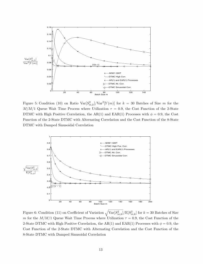
For each test process, Figure 2 displays the lag-1 correlation between batch means as a functionof the batch size m. For valid application of the NOBM method, the lag-1 correlation of the batchmeans should be near zero. Figure 2 shows that highly correlated processes can require very largebatch sizes to achieve a sufficiently small correlation between adjacent batch means. Figures 3–6 reveal that highly correlated processes can also require large batch sizes to satisfy the NOBMmoment conditions (8)–(11).
4.1 Discrete Time Markov Chains
The first test case consists of a “cost” process defined on a finite-state, irreducible, aperiodic DTMC.If the underlying (d+ 1)-state DTMC {Ui : i = 0, 1, . . .} with state space {0, 1, . . . , d} has one-steptransition probability matrix P, steady-state probability vector π = (π0, π1, . . . , πd), and associated(d + 1) × (d + 1) matrix
Π =
π
π...π
, (20)
and if the initial state U0 is sampled from the steady-state distribution π, then the correspondingcost process {Xi = h(Ui) : i = 0, 1, ...} is covariance stationary, where h(·) : {0, 1, . . . , d} → R
specifies the cost of visiting each state of the underlying chain. Following the approach used byHazen and Pritsker (1980) for continuous time Markov chains, we obtained the following expressionfor the lag-q covariance of the cost process {Xi}
γ(q) = hT∆ (Pq − Π) h for q = 0,±1,±2, . . . , (21)
where h ≡ [h(0), h(1), . . . , h(d)]T and ∆ ≡ diag (π0, π1, · · · , πd).Now if the one-step transition probability matrix P has distinct real eigenvalues, then the qth
power of P may be calculated as
Pq = VΛqV−1, (22)
where V = [v0,v1, · · · ,vd] is the (d + 1) × (d + 1) matrix of right eigenvectors of P and Λ =diag(λ0, λ1, . . . , λd) is the diagonal matrix of associated eigenvalues (Hadley 1961).
10
0 10 20 30 40 50 60 70 80 90 100−1
−0.8
−0.6
−0.4
−0.2
0
0.2
0.4
0.6
0.8
1
Lag
Cor
rela
tion
o−−−M/M/1 QWT
*−−−DTMC High Pos. Corr.
x−−−AR(1) and EAR(1) Processes
DTMC Alt. Corr.
−−−−DTMC Sinusoidal Corr.
· · ·
Figure 1: Lag q Correlation Corr(Xi, Xi+q) = γ(q)/σ2X of Observations of the Wait Times in the
M/M/1 Queue with Utilization τ = 0.9, the Cost Function of the 2-State DTMC with HighPositive Correlation, the AR(1) and EAR(1) Processes with φ = 0.9, the Cost Function of the2-State DTMC with Alternating Correlation and the Cost Function of the 8-State DTMC withDamped Sinusoidal Correlation
50 100 150 200 250 300 350 400 450 500−0.8
−0.6
−0.4
−0.2
0
0.2
0.4
0.6
0.8
1
Batch Size m
Lag
1 C
orre
latio
n
o−−−M/M/1 QWT
*−−−DTMC High Pos. Corr.
x−−−AR(1) and EAR(1) Processes
DTMC Alt. Corr.
−−−−DTMC Sinusoidal Corr.
· · ·
Figure 2: Lag 1 Correlation of the Batch Means with Batches of Size m for the Wait Times inthe M/M/1 Queue with Utilization τ = 0.9, the Cost Function of the 2-State DTMC with HighPositive Correlation, the AR(1) and EAR(1) Processes with φ = 0.9, the Cost Function of the2-State DTMC with Alternating Correlation and the Cost Function of the 8-State DTMC withDamped Sinusoidal Correlation
11
kVar[Y (m,k) ]Var[Y (m)]
10 20 30 40 50 60 70 80 90 1000
5
10
15
20
25
Batch Size m
o−−−M/M/1 QWT
*−−−DTMC High Pos. Corr.
x−−−AR(1) and EAR(1) Processes
−−−DTMC Alt. Corr.
−−−DTMC Sinusoidal Corr.
!"
Figure 3: Condition (8) on Ratio kVar[Y (m, k)]/Var[Y (m)] for k = 30 Batches of Size m for WaitTimes in the M/M/1 Queue with Utilization τ = 0.9, the Cost Function of the 2-State DTMCwith High Positive Correlation, the AR(1) and EAR(1) Processes with φ = 0.9, the Cost Functionof the 2-State DTMC with Alternating Correlation and the Cost Function of the 8-State DTMCwith Damped Sinusoidal Correlation
E[S2m,k]
Var[Y (m)]
10 20 30 40 50 60 70 80 90 1000
0.2
0.4
0.6
0.8
1
o−−−M/M/1 QWT
*−−−DTMC High Pos. Corr.
x−−−AR(1) and EAR(1) Processes
−−−DTMC Alt. Corr.
−−−DTMC Sinusoidal Corr.
Batch Size m
!
"
Figure 4: Condition (9) on Ratio E[S2m,k]/Var[Y (m)] for k = 30 Batches of Size m for Wait Times
in the M/M/1 Queue with Utilization τ = 0.9, the Cost Function of the 2-State DTMC with HighPositive Correlation, the AR(1) and EAR(1) Processes with φ = 0.9, the Cost Function of the2-State DTMC with Alternating Correlation and the Cost Function of the 8-State DTMC withDamped Sinusoidal Correlation
12
Var[S2m,k]
Var2[Y (m)]
20 40 60 80 100 120 1400
0.02
0.04
0.06
0.08
0.1
0.12
0.14
0.16
0.18
Batch Size m
2/(k−1)
o−−−M/M/1 QWT
*−−−DTMC High Corr.
x−−−AR(1) and EAR(1) Processes
−−−DTMC Alt. Corr.
−−−DTMC Sinusoidal Corr.
!"
Figure 5: Condition (10) on Ratio Var[S2m,k]/Var2[Y (m)] for k = 30 Batches of Size m for the
M/M/1 Queue Wait Time Process where Utilization τ = 0.9, the Cost Function of the 2-StateDTMC with High Positive Correlation, the AR(1) and EAR(1) Processes with φ = 0.9, the CostFunction of the 2-State DTMC with Alternating Correlation and the Cost Function of the 8-StateDTMC with Damped Sinusoidal Correlation
√Var[S2
m,k]
E[S2m,k]
20 40 60 80 100 120 140 160 180 2000
0.1
0.2
0.3
0.4
0.5
0.6
0.7
0.8
0.9
1
Batch Size m
o−−−M/M/1 QWT
*−−−DTMC High Pos. Corr.
x−−−AR(1) and EAR(1) Processes
−−−DTMC Alt. Corr.
−−−DTMC Sinusoidal Corr.
√2/(k − 1)
!"
Figure 6: Condition (11) on Coefficient of Variation√
Var[S2m,k]/E[S2
m,k] for k = 30 Batches of Sizem for the M/M/1 Queue Wait Time Process where Utilization τ = 0.9, the Cost Function of the2-State DTMC with High Positive Correlation, the AR(1) and EAR(1) Processes with φ = 0.9, theCost Function of the 2-State DTMC with Alternating Correlation and the Cost Function of the8-State DTMC with Damped Sinusoidal Correlation
13
We also derived a matrix-analytic expression for the SSVC of a cost process {Xi} defined on afinite-state DTMC. The following theorem provides a computational formula for σ2. See Appendix3 or Steiger (1999) for a proof of this result.
Theorem 2 If the (d+1)-state DTMC {Ui : i = 0, 1, . . .} has one-step transition probability matrixP and associated (d+ 1) × (d+ 1) matrix Π defined by (20), then the SSVC of the associated costprocess {Xi = h(Ui) : i = 0, 1, ...} is given by
σ2 = hT∆[Id+1 − Π + 2 (Id+1 − P + Π)−1 (P − Π)
]h. (23)
For our analysis, we chose three DTMCs, each having a substantially different correlation func-tion for the associated cost process. The first cost process is defined on a simple two-state DTMC{Ui : i = 0, 1, . . .} with transition probability matrix
P =
( 0 1
0 0.25 0.751 0.75 0.25
)
and the cost vector
h =( 0 1
5 10). (24)
The cost process {Xi : i = 0, 1, . . .} possesses an alternating positive and negative correlationfunction, as illustrated in Figure 1.
The second test case is also based on a two-state DTMC, but the associated cost process hasa large positive correlation function that decays very slowly to zero. This case uses the same costvector (24) as the first case, but the underlying DTMC {Ui} has transition probability matrix
P =
( 0 1
0 0.99 0.011 0.01 0.99
). (25)
The third test case is based on an eight-state DTMC {Ui} so that the associated cost process{Xi} has a correlation function that resembles a damped sine wave. The third DTMC {Ui} wasdesigned to loosely represent some sort of cyclical behavior, where the chain repeatedly tends to
14
visit all its states in order. The probability transition matrix for this chain is
The cost vector associated with the eight states of this chain is
h =( 0 1 2 3 4 5 6 7
0 5 10 15 20 25 30 35).
The transition probability matrices for these three DTMCs have distinct real eigenvalues, sowe used MATLAB (Hanselman and Littlefield 1997) to compute the eigenvalues and their corre-sponding eigenvectors. We then computed the covariances of the original processes as well as thecovariances for the batch means processes using the matrix-analytic equations (21) and (22).
4.2 M/M/1 Queue Waiting Times
Next we examined a test process consisting of the sequence of customer waiting times {Xi : i =1, 2, . . .} in the M/M/1 queue. Letting τ = λ/µ denote the server utilization (or traffic intensity),where λ is the arrival rate and µ is the service rate, we see that the mean queue waiting time is
µX =λ
µ(µ− λ);
and the variance of the waiting time is
σ2X =
λ(2µ− λ)µ2 (µ− λ)2
.
The marginal distribution of each waiting time in steady-state operation is mixed with c.d.f.
FX(x) =
0, x < 0,
1 − τ, x = 0,
1 − τe−(µ−λ)x, x > 0.
Thus each waiting time is zero with probability 1−τ ; and with probability τ , it is exponential withmean (µ − λ)−1. The lag-q covariance, γ(q), for the waiting time process in the M/M/1 queue isgiven by
γ(q) =1 − τ2
2πλ2
∫ 4τ(1+τ)−2
0zq+3/2 [4τ(1 + τ)−2 − z
]1/2 (1 − z)−3 dz for q = 0,±1,±2, . . . (26)
15
(Song and Schmeiser 1995), where τ < 1. The SSVC is given by
σ2 =τ3(τ3 − 4τ2 + 5τ + 2
)λ2 (1 − τ)4
(Daley 1968). We used MATLAB (Hanselman and Littlefield 1997) to evaluate numerically theintegral in (26) for utilization τ = 0.9. As can be seen from Figures 3–6, the rate of convergence tothe moment conditions is extremely slow.
4.3 Autoregressive Process
We also investigated the autoregressive process of order one (that is, AR(1)), which is defined bythe iterative relation
Xi = µX + ϕ(Xi−1 − µX) + εi for i = 1, 2, . . . , (27)
where |ϕ| < 1 and the εi’s are i.i.d. normal with mean zero and variance σ2ε so that the Xi’s have
mean µX and variance σ2X = σ2
ε /(1−ϕ2). To ensure that (27) defines a stationary process, we tookX0 ∼ N(µX , σ2
X). The lag-q covariance for the AR(1) process is
γ(q) = σ2Xϕ
|q| = σ2εϕ
|q|/(1 − ϕ2) for q = 0,±1,±2, . . . ; (28)
and the SSVC is given by
σ2 = σ2X
(1 + ϕ
1 − ϕ
)=
σ2ε
(1 − ϕ)2(29)
(Box, Jenkins, and Reinsel 1994).
4.4 Exponential Autoregressive Process
Finally we examined the exponential autoregressive process of order one (that is, EAR(1)), whichis defined by the iterative relation
where 0 < ϕ < 1 and the εi’s are i.i.d. exponential with rate λ = 1/σX so that the Xi’s have mean µXand variance σ2
X = 1/λ2. As in the AR(1) process, the covariance function for the EAR(1) processhas the form (28); and the corresponding SSVC is obviously given by (29). By sampling X0 froman exponential distribution with mean 1/λ, we ensured that the EAR(1) process is stationary withthe same exponential marginal distribution. This means larger batch sizes should be required tosatisfy the assumption that the batch means are normally distributed as compared to, for instance,the AR(1) process, where the marginal distribution of each Xi is normal. In the case selected, wechose ϕ = 0.9 and λ = 0.5.
16
5. Monte Carlo Analysis of Components of Batch Means t-Ratio
for Selected Cases
After we evaluated numerically the moment conditions for various batch sizes as described in theprevious section, we simulated the six selected test processes to study the empirical convergenceto the distributional requirements. We looked at the distributions of the numerator and squareddenominator of the NOBM t-ratio (5) separately, and we compared the empirical distributions ofthese target statistics for various batch sizes to the associated limiting distributions. Figures 7–10display the Monte Carlo results obtained for the M/M/1 queue waiting times and for the AR(1)process. Steiger (1999) presents the complete Monte Carlo results for all six test cases.
The number of batches was fixed at k = 30, and the initial batch size was usually chosen to bem = 8. For each selected process, the batch size was increased until each observed frequency distri-bution (as depicted by a histogram and by a plot of the empirical c.d.f. based on 2,000 replicationsof the target statistic) was judged to approximate adequately the associated limiting distribution(as depicted by the corresponding p.d.f. and c.d.f., which are overlaid on their respective plots). Allsimulations were started by sampling the selected process from its steady-state distribution; andthus all simulation-generated data sets were realizations of stationary stochastic processes.
The “worst” test case—that is, the one requiring the largest batch size (m = 4096) for theobserved distributions to achieve adequate convergence to their theoretical counterparts—was thecase of M/M/1 waiting times with server utilization τ = 0.9. It should be noted that this case hasthe most slowly decaying correlation function as well as a mixed marginal distribution with an ex-ponential tail. Both of these factors cause serious deviations from the assumptions of independenceand normality of the batch means when the batch size is small.
In the other five test cases, the largest batch size required for reasonable convergence to thedesired limiting distributions was m = 512. This was the case of the highly correlated DTMC-basedcost process defined by (24) and (25). Again the slowly decaying correlation (see Figure 1) and thediscreteness of the underlying distribution tend to result in slow convergence to the desired limitingproperties.
An interesting insight to be gained from these investigations was that often at relatively smallbatch sizes, even though the numerator of the NOBM t-ratio (5) displayed a variance that differedsubstantially from the limiting value of one, the empirical distribution of the numerator was stillnearly bell-shaped. In view of the asymptotic moment requirement (8), this observation suggeststhat the dependency among the batch means remained a serious problem long after the batch sizewas large enough to ensure approximate normality of the numerator of the NOBM t-ratio.
6. Conclusions and Recommendations
Both the theoretical and empirical convergence properties of the batch means process gleaned fromour experimentation with the DTMC-based cost processes, the AR(1) process, and the EAR(1)
17
−5 0 50
0.1
0.2
0.3
0.4
0.5
Numerator
Relat
ive F
requ
ency
AR(1) m=16
−5 0 50
0.1
0.2
0.3
0.4
0.5
Numerator
Relat
ive F
requ
ency
M/M/1 QWT m=16
−5 0 50
0.1
0.2
0.3
0.4
0.5
Numerator
Relat
ive F
requ
ency
AR(1) m=64
−5 0 50
0.1
0.2
0.3
0.4
0.5
Numerator
Relat
ive F
requ
ency
M/M/1 QWT m=4096
Figure 7: Relative Frequency of the Numerator of the t-Statistic (5) Based on 2000 Replicationsof the AR(1) Process (30) with ϕ = 0.9 for k = 30 Batches of Size m = 16 and m = 64 and theM/M/1 Queue Wait Time Process where Utilization τ = 0.9 for k = 30 Batches of Size m = 16and m = 4096
−5 0 50
0.1
0.2
0.3
0.4
0.5
0.6
0.7
0.8
0.9
1
Numerator
Cu
mu
lative
Re
lative
Fre
qu
en
cy
− −M/M/1 QWT m=4096
+AR(1) m=64
−5 0 50
0.1
0.2
0.3
0.4
0.5
0.6
0.7
0.8
0.9
1
Numerator
Cu
mu
lative
Re
lative
Fre
qu
en
cy
− −M/M/1 QWT m=16
+AR(1) m=16
Figure 8: Cumulative Relative Frequency of the Numerator of the t-Statistic (5) Based on 2000Replications of the AR(1) Process (30) with ϕ = 0.9 for k = 30 Batches of Size m = 16 and m = 64and the M/M/1 Queue Wait Time Process where Utilization τ = 0.9 for k = 30 Batches of Sizem = 16 and m = 4096
18
0 20 40 60 80 1000
0.01
0.02
0.03
0.04
0.05
0.06
Denominator
Rela
tive
Freq
uenc
y
AR(1) m=16
0 20 40 60 80 1000
0.01
0.02
0.03
0.04
0.05
0.06
Denominator
Rela
tive
Freq
uenc
y
M/M/1 QWT m=16
0 20 40 60 80 1000
0.01
0.02
0.03
0.04
0.05
0.06
Denominator
Rela
tive
Freq
uenc
y
AR(1) m=64
0 20 40 60 80 1000
0.01
0.02
0.03
0.04
0.05
0.06
Denominator
Rela
tive
Freq
uenc
y
M/M/1 QWT m=4096
Figure 9: Relative Frequency of the Squared Denominator of the t-Statistic (5) Based on 2000Replications of the AR(1) Process (30) with ϕ = 0.9 for k = 30 Batches of Size m = 16 and m = 64and the M/M/1 Queue Wait Time Process where Utilization τ = 0.9 for k = 30 Batches of Sizem = 16 and m = 4096
0 20 40 60 80 1000
0.1
0.2
0.3
0.4
0.5
0.6
0.7
0.8
0.9
1
Denominator
Cu
mu
lative
Re
lative
Fre
qu
en
cy
+ AR(1) m=16
− −M/M/1 QWT m=16
0 20 40 60 80 1000
0.1
0.2
0.3
0.4
0.5
0.6
0.7
0.8
0.9
1
Denominator
Cu
mu
lative
Re
lative
Fre
qu
en
cy
+ AR(1) m=64
− −M/M/1 QWT m=4096
Figure 10: Cumulative Relative Frequency of the Squared Denominator of the t-Statistic (5) Basedon 2000 Replications of the AR(1) Process (30) with ϕ = 0.9 for k = 30 Batches of Size m = 16 andm = 64 and the M/M/1 Queue Wait Time Process where Utilization τ = 0.9 for k = 30 Batchesof Size m = 16 and m = 4096
19
process lead us to suspect that often the joint distribution of the batch means converges to anapproximately multivariate normal distribution at smaller batch sizes than are required to achieveapproximate independence of the batch means. The distributions of the numerator of the NOBMt-statistic (5) for these three types of processes are symmetric even at small batch sizes. The plotsof the observed distributions of the numerator overlaid with the theoretical standard normal densityshow that at small batch sizes the observed distributions display an incorrect variance (scaling)but are nearly bell-shaped. The distributions of the squared denominator in these cases closelyresemble the appropriate χ2
k−1/(k − 1) distribution. Of the cases we studied, only in the M/M/1queue waiting time process did we find marked asymmetry in the distribution of the numeratorof the NOBM t-statistic (5) together with marked deviation from the limiting distribution of thedenominator at moderate batch sizes.
In processes having strong positive dependence, a batch size that is too small (resulting in batchmeans with large positive correlations) causes the classical batch means method to underestimatethe variance of the grand mean Y (m, k), resulting in CIs that possess inadequate coverage prob-ability. Conversely, in processes with alternating correlation structure, the classical batch meansestimator S2
m,k/k may overestimate Var[Y (m, k)]. In either case, the resulting CI may not possessthe desired coverage probability.
The results of our numerical and Monte Carlo investigations of the convergence properties ofbatch means led us to the development of the Automated Simulation Analysis Procedure (ASAP),an improved NOBM algorithm for a constructing a CI on the expected response of a steady-state simulation that satisfies a user-specified absolute or relative precision requirement. ASAPoperates as follows: the batch size is progressively increased until either (a) the batch means passthe von Neumann test for independence, and then ASAP delivers the classical NOBM confidenceinterval (6); or (b) the batch means pass the Shapiro-Wilk test for multivariate normality, andthen ASAP delivers an adjusted confidence interval. The latter adjustment is based on an invertedCornish-Fisher expansion for the classical NOBM t-ratio (5), where the terms of the expansion areestimated via an autoregressive–moving average time series model of the batch means. An extensiveexperimental performance evaluation demonstrates the effectiveness of ASAP (Steiger 1999; Steigerand Wilson 1999; Steiger and Wilson 2000a, b).
Appendix 1: Proof of Theorem 1
For a fixed batch count k, the following development characterizes the asymptotic behavior of thek-dimensional vector of batch means under fairly general conditions as the batch size m → ∞.
Definition 1 Let D denote the space of functions on [0, 1] that are right-continuous and haveleft-hand limits. For Q,Q′ ∈ D, let d(Q,Q′) denote the Skorohod metric on D (Billingsley 1968)—that is, if Λ denotes the class of strictly increasing, continuous mappings of [0, 1] onto itself, then
20
d(Q,Q′) is defined to be the infimum of those positive δ for which there exists λ ∈ Λ such that
supt|λt− t| ≤ δ
supt|Q(t) −Q′(λt)| ≤ δ
}. (A1)
Note that if λ ∈ Λ, then so does λ′ ≡ λ−1; and as t runs from 0 to 1, so does t′ ≡ λt. Alsosupt|λt− t| = supt′ |λ′t′ − t′| and supt|Q(t) −Q′(λt)| = supt′ |Q(λ′t′) −Q′(t′)|. Thus we see that asa completely equivalent alternative to the definition (A1), we may take d(Q,Q′) to be the infimumof all δ > 0 for which there exists λ′ ∈ Λ such that
supt′ |λ′t′ − t′| ≤ δ
supt′ |Q(λ′t′) −Q′(t′)| ≤ δ
}. (A2)
Definition 2 The function ψ : D → Rk is defined as follows: for every Q ∈ D,
ψ (Q(·, ω)) ≡√k
[Q
(1k, ω
)−Q(0, ω) , Q
(2k, ω
)−Q
(1k, ω
), . . . ,
Q(1, ω) −Q
(k − 1k
, ω
)].
Definition 3 Let Dk ⊂ D denote the subset of functions in D that are continuous at the multiplesof 1/k in the unit interval,
Dk ≡{Q ∈ D : Q
(j
k
)= Q
(j
k−)
for j = 1, 2, . . . , k}.
Definition 4 Let {Xi : i = 1, 2, . . .} be a stationary, φ-mixing process with: E[X0] = µX ;Var[X0] < ∞; mixing coefficients {φi} satisfying
∑∞i=1
√φi < ∞; and SSVC σ2 satisfying 0 <
σ2 < ∞. Let σ ≡√σ2, and for each positive interger n, define Un ∈ D as
Un(t, ω) ≡ 1σ√n
�nt∑i=1
[Xi(ω) − µX ] for t ∈ [0, 1].
Theorem 3 If D, ψ, Dk, and Un are specified by Definitions 1, 2, 3, and 4 respectively, then:
1. ψ(·) is continuous at every Q ∈ Dk ⊂ D.
2. As n → ∞, ψ(Un(·, ω)) converges in distribution to a standard k-variate normal distribution,
ψ(Un(·, ω)) D−→n→∞ Nk(0k, Ik). (A3)
Proof of 1. Let ε > 0 be an arbitrarily small positive number and choose Q ∈ Dk arbitrarily. Todemonstrate the continuity of ψ(·) at Q, we will show the existence of an η = η(Q, ε, k) > 0 suchthat if Q′ ∈ D and d(Q,Q′) < η, then ‖ψ(Q) − ψ(Q′)‖2 < 4ε
√k.
Since Q ∈ Dk, by Definition 3 we can find an η1 = η1(Q, ε, k) > 0 such that,
From (A9), (A10), and (A11) it follows that |dj | ≤ 2ε for j = 0, 1, . . . , k; and from (A7) and (A8),it follows immediately that ‖ψ(Q) −ψ(Q′)‖2
2 ≤ 16ε2k. Since we selected Q ∈ Dk arbitrarily and wetook Q′ ∈ D such that d(Q,Q′) ≤ δ, we have established continuity of the function ψ(·) at everyQ ∈ Dk.
22
Proof of 2. By Theorem 20.1 of Billingsley (1968),
Un(·, ω) D−→n→∞ B(·, ω). (A12)
Since ψ(·) is continuous at every point in Dk and the Brownian motion process {B(t, ω) : 0 ≤ t ≤ 1}has a continuous sample path for each sample point ω in the underlying probability space (see, forexample, p. 64 of Billingsley 1968), it follows that
Pr{B(·, ω) ∈ D − Dk} = 0. (A13)
Displays (A12) and (A13) together with the continuous mapping theorem (Corollary 1 of Theorem5.1, Billingsley 1968) yield
ψ(Un(·, ω)) D−→n→∞ ψ(B(·, ω)). (A14)
It follows from standard properties of the increments of Brownian motion (see, for example, p. 343of Karlin and Taylor (1975)) that
Finally, we establish the main result (7) of Theorem 1 when in the NOBM method we fixthe batch count k, we take the overall sample size n = km, and we let the batch size m → ∞.Expressing ψ(Un(·, ω)) in terms of centered partial sums of the form
for 1 ≤ i, j, u, 2 ≤ k. At θ = 0, M = 1 and L� = 0 for 2 = 1, . . . , k. Therefore evaluating the partialderivatives at t = 0 yields the following values for the mixed moments:
Since the SSVC, σ2, is the sum of the covariances at all lags, from (21) we have
σ2 = hT∆
{Id+1 − Π + 2
∞∑�=1
(P� − Π
)}h. (A17)
It is easy to prove by induction that
(P − Π)� = P� − Π for 2 = 1, 2, . . . . (A18)
It follows that lim�→∞ (P − Π)� = lim�→∞ P� − Π = Π − Π = 0; and thus Theorem 1.11.1 ofKemeny and Snell (1960) ensures that
(Id+1 − P + Π)−1 =∞∑�=0
(P − Π)� . (A19)
If we take G ≡∑∞�=1 (P − Π)� , then it follows immediately that
(P − Π) G =∞∑�=2
(P − Π)� = G − (P − Π) . (A20)
Using (A18) and (A19) to solve (A20) for G, we have
G = (Id+1 − P + Π)−1 (P − Π) =∞∑�=1
(P� − Π
). (A21)
Combining (A17) and (A21), we finally obtain the desired result (23).
Acknowledgments
The authors thank the Michael Taaffe, the Area Editor, and the referees for several suggestionsthat substantially improved this paper. The authors also thank David Goldsman (Georgia Instituteof Technology) and Stephen D. Roberts (North Carolina State University) for many enlighteningdiscussions on this paper.
References
Anderson, T.W. 1971. The Statistical Analysis of Time Series. John Wiley & Sons, New York.Billingsley, P. 1968. Convergence of Probability Measures. John Wiley & Sons, New York.Box, G.E.P., G.M. Jenkins, G.C. Reinsel. 1994. Time Series Analysis: Forecasting and Control,
Third Edition. Holden-Day, San Francisco.Daley, D.J. 1968. The serial correlation coefficients of waiting times in a stationary single server
queue. Journal of the Australian Mathematical Society 8 683–699.
25
Fishman, G.S. 1978. Grouping observations in digital simulation. Management Science 24 510–521.
Hadley, G. 1961. Linear Algebra. Addison-Wesley, Reading, MA.Hanselman, D., B. Littlefield. 1997. The Student Edition of MATLAB: Version 5, User’s Guide/The
MathWorks, Inc. Prentice-Hall, Upper Saddle River, NJ.Hazen, G.B., A.A.B. Pritsker. 1980. Formulas for the variance of the sample mean in finite state
Markov processes. Journal of Statistical Computation and Simulation 12 25–40.Kang, K., D. Goldsman. 1990. The correlation between mean and variance estimators in computer
simulation. IIE Transactions 22 15–23.Karlin, S., H.M. Taylor. 1975. A First Course in Stochastic Processes, Second Edition. Academic
Press, New York.Kemeny, J.G., J.L. Snell. 1960. Finite Markov Chains. D. Van Nostrand and Co., Princeton, NJ.Law, A.M., W.D. Kelton. 2000. Simulation Modeling and Analysis, 3d ed. McGraw-Hill, New
York.Munoz, D.F., P.W. Glynn. 1997. A batch means methodology for estimation of a nonlinear function
of a steady-state mean. Management Science 43 1121–1135.Sargent, R.G., K. Kang, D. Goldsman. 1992. An investigation of finite-sample behavior of confi-
Science 41 110–123.Steiger, N.M. 1999. Improved batching for confidence interval construction in steady-state simu-
lation. Ph.D. Dissertation, Department of Industrial Engineering, North Carolina State Uni-versity, Raleigh, NC. http://www.lib.ncsu.edu/etd/public/etd-19231992992670/etd.pdf[accessed January 15, 2001].
Steiger, N.M., J.R. Wilson. 1999. Improved batching for confidence interval construction in steady-state simulation. P.A. Farrington, H.B. Nembhard, D.T. Sturrock, and G.W. Evans, eds.Proceedings of the 1999 Winter Simulation Conference. Institute of Electrical and Electron-ics Engineers, Piscataway, NJ. 442-451. http://www.informs-cs.org/wsc99papers/061.PDF[accessed May 11, 2000].
Steiger, N. M., J. R. Wilson. 2000a. Experimental performance evaluation of batch-means proce-dures for simulation output analysis. R.R. Barton, J.A. Joines, K. Kang, and P.A. Fishwick,eds. Proceedings of the 2000 Winter Simulation Conference. Institute of Electrical and Electron-ics Engineers, Piscataway, NJ. 627–636. http://www.informs-cs.org/wsc00papers/084.PDF[accessed January 6, 2000].
Steiger, N. M., J. R. Wilson. 2000b. An improved batch means procedure for simulation outputanalysis. Technical Report, Department of Industrial Engineering, North Carolina State Uni-versity, Raleigh, NC. ftp://ftp.ncsu.edu/pub/eos/pub/jwilson/asaporv12.pdf [accessedJune 18, 2000].


![PFDet: 2nd Place Solution to Open Images Challenge 2018 ... · Batch normalization (BN) is used ubiquitously to speed up convergence of training [5]. We use multi-node batch normalization](https://static.documents.pub/doc/80x56/60073f198c877074df24f503/pfdet-2nd-place-solution-to-open-images-challenge-2018-batch-normalization.jpg)


