Convexiﬁcation of Power Flow Equations for Power …lavaei/SE_J_2016.pdf · Convexiﬁcation of...

1

Convexification of Power Flow Equations for Power Systemsin Presence of Noisy Measurements

Ramtin Madani, Javad Lavaei and Ross Baldick

Abstract—This paper is concerned with the power systemstate estimation (PSSE) problem that aims to find the unknownoperating point of a power network based on a given set ofmeasurements. We first study the power flow (PF) problem as animportant special case of PSSE, which is known to be non-convexand NP-hard in the worst case. To this end, we propose a setof semidefinite programs (SDPs) with the property that they allsolve the PF problem as long as the voltage angles are relativelysmall. Associated with each SDP, we explicitly characterize theset of all complex voltages that can be recovered via that convexproblem. As a generalization, the design of an SDP problem thatrecovers multiple nominal points and a neighborhood aroundeach point is also cast as a convex program. The results are thenextended to the PSSE problem, where the measurements usedin the PF problem are subject to noise. A two-term objectivefunction is employed for each convex program developed for thePSSE problem: (i) one term accounting for the non-convexityof the power flow equations, (ii) another one for estimating thenoise levels. An upper bound on the estimation error is derivedwith respect to the noise level and the proposed techniquesare demonstrated on multiple test systems, including a 9241-bus European network. Although the focus of the paper is onpower networks, the results developed in this work apply to everyarbitrary state estimation problem with quadratic measurementequations.

I. INTRODUCTION

Consider a group of generators (i.e., sources of energy),which are connected to a group of electrical loads (i.e.,consumers) via an electrical power network. This networkcomprises a set of transmission lines connecting various nodesto each other (e.g., a generator to a load). At each nodeof the network, the associated external devices (loads andgenerators) exchange a net complex electrical power with thenetwork, where the real and imaginary parts of this complexpower are called active and reactive powers. The active poweris a measure of the short-term average power delivered toloads that is able to do useful work, whereas the reactivepower is a measure of the back-and-forth flow of power inthe network between electric and magnetic fields. The nodalcomplex powers induce active and reactive powers over alllines of the network, which are referred to as line flows. The

Ramtin Madani is with the Department of Electrical Engineering, Universityof Texas at Arlington ([email protected]). Javad Lavaei is with theDepartment of Industrial Engineering and Operations Research, Universityof California, Berkeley ([email protected]). Ross Baldick is with theDepartment of Electrical and Computer Engineering, University of Texas atAustin ([email protected]). This work was supported by DARPA YFA,ONR YIP Award, DARPA Young Faculty Award, AFOSR YIP Award, NSFCAREER Award 1351279, and NSF EECS Awards 1406894 and 1406865.Parts of this work have appeared in the conference papers “Ramtin Madani,Javad Lavaei and Ross Baldick, Convexification of power flow problem overarbitrary networks, IEEE Conference on Decision and Control, 2015”, and“Ramtin Madani, Morteza Ashraphiojuo, Javad Lavaei and Ross Baldick,Power system state estimation with a limited number of measurements, IEEEConference on Decision and Control, 2016”.

complex flow entering a line could differ from the flow leavingthe line at the other end since transmission lines are lossyin practice. On the other hand, each node of the network(called a bus) is associated with a complex number, namednodal voltage. To describe the relationship among all nodalpowers and line flows, it is possible to write each of theseparameters as a quadratic function of nodal voltages usingpower flow equations. The set of all nodal complex voltagesof a power network is referred to as the state of the system.The power flow (PF) problem involves solving power flowequations in order to find the state of the system, given a setof noiseless measurements. These measurements are usuallya subset of voltage magnitudes, nodal active powers, nodalreactive powers, active line flows and reactive line flows.

A. Power Flow Problem

Power Flow equations are central to the analysis and opera-tion of power systems, based upon which several optimizationproblems are built. These problems include optimal powerflow, state estimation, security-constrained optimal power flow,unit commitment, network reconfiguration, and transmissionswitching [1]–[4]. However, it is well-known that solvingthese equations, namely the PF problem, is NP-hard for bothtransmission and distribution networks due to its reductionto the subset sum problem [5], [6]. The recent paper [7]shows the strong NP-hardness of this problem for certain typesof systems. The nonlinearity of the power flow equations isimposed by the laws of physics, and is a major impediment tothe efficient, optimal and reliable operation of power systems.

Since 1962, several linearization and local search algorithmshave been developed for solving power flow equations, and thecurrent practice in the power industry relies on linearizationand/or Newton’s method (depending on the time scale andwhether the problem is solved for planning or real-time oper-ation) [8]–[10]. Traditional methods based on the linearizationof power flow equations do not typically capture importantquantities such as voltage magnitudes, thermal losses andreactive flows, which make these techniques less appealing forapplications such as voltage control. As a result, great efforthas been devoted to developing modified linear programmingmodels that incorporate reactive power and voltage magnitudes[11], [12]. Another major focus of the existing literature forsolving power flow equations has been on homotopy continua-tion methods that are widely applied to the PF problem [13]–[15]. As argued in [16], earlier homotopy-based techniqueslack performance guarantees, have scalability issues, and maynot always find all solutions of the PF problem. Nevertheless,new homotopy algorithms have been recently introduced in[17] and [18] that are provably capable of finding all feasible

2

solutions and attempt to ameliorate the issue of scalabilitythrough parallelization. Other approaches for tackling thenonlinearity of power flow equations include Groebner basistechniques and interval based methods [19]–[21]. The recentpapers [22] and [23] propose upper bounds on the number ofsolutions for the PF problem based on the network topology.

In this paper, we exploit the semidefinite programmingrelaxation technique to handle the non-convexity of thePF problem. Semidefinite programming (SDP) is a subfieldof convex optimization, which has received a considerableamount of attention in the past two decades [24]–[27]. TheSDP relaxation technique is a powerful method for tacklingquadratic nonlinearities, which has been proven to be effectivein the convexification of several hard optimization problems invarious areas, including graph theory, approximation theory,quantum mechanics, neural networks, communication net-works, and power systems [28]–[33]. SDP relaxation meth-ods have been successfully used for real-world applicationssuch as radar code design, multiple-input and multiple-output(MIMO) beamforming, error-correcting codes, magnetic res-onance imaging (MRI), data training, and portfolio selection,among many others [34]–[37]. Several papers have evaluatedthe performance of SDP relaxations for various problems, byinvestigating the approximation ratio and the maximum rankof SDP solutions [38]–[42]. Moreover, different global opti-mization techniques for polynomial optimization have beenbuilt upon SDP relaxations [32], [43]–[46].

Our first contribution is related to the PF problem. To handlethe non-convexity of this feasibility problem, we propose aclass of convex optimization programs in the form of SDPs.We derive an exact recovery region for each convex programin the proposed SDP class. This means that the solution ofthe PF problem can be found using SDP if and only if itbelongs to the associated recovery region. Moreover, we provethat if the voltage angles are small enough, the classical PFproblem can be solved precisely using the proposed SDPproblems, and this result does not make any assumption onthe network topology whatsoever. Note that voltage angles areoften small in practice due to practical considerations, whichhas two implications: (i) linearization would be able to find anapproximate solution, (ii) Newton’s method would converge byinitializing all voltage angles at zero. Linearization techniquesoffer low-complexity approximate models that can provideinsights into power systems, whereas Newton’s method is anattractive numerical algorithm that has been used in the powerindustry for many years [47], [48]. Some of the advantages ofthe SDP technique over the aforementioned approaches are asfollows:• A one-time linearization of the power flow equations

(known as DC modeling) solves the PF problem approx-imately by linearizing the laws of physics. However, theproposed SDP problem finds the correct solution (withany arbitrary precision) as long as it belongs to thecorresponding recovery region.

• The basin of attraction of Newton’s method is chaotic andhard to characterize in general, but the recovery regionof the proposed SDP problem is explicitly characterizablevia matrix inequalities [49].

• The SDP relaxation provides a convex model for the PFproblem, independent of what numerical algorithm willbe used to solve it.

• As will be verified on benchmark systems later in thispaper, the proposed SDP relaxation has a higher successrate than Newton’s method.

Our approach relies on converting the feasibility PF probleminto a convex program in two steps: (i) PF is transformed intoan optimization problem by augmenting PF with a suitableobjective function, (ii) the resulting non-convex problem isrelaxed to an SDP problem. The designed objective functionis not unique and there are infinitely many choices for thisfunction. The question arises as to whether any of theseobjective functions added to the PF problem would have aphysical meaning. To address this problem, we show thatone such function is the sum of squares of the nodal currentmagnitudes, which indirectly accounts for the loss in thenetwork. Note that each objective function produces its ownrecovery region and therefore it is not always beneficial touse a physically meaningful objective function instead of asynthetically designed function. In this paper, we also studythe problem of selecting the best objective function.

B. Power Systems State Estimation

Power system state estimation (PSSE) is the problem ofdetermining the operating point of an electrical network basedon the given model and the measurements obtained fromsupervisory control and data acquisition (SCADA) systems[50]. Notice that PSSE is built upon the PF problem byreplacing noiseless specifications with noisy measurements,and therefore it is also a nonconvex problem. In order toadapt the proposed approach for the PF problem to PSSE, weadopt a penalized convex relaxation approach similar to [51],where the measurement equations are softly penalized in theobjective as opposed to being imposed as equality constraints.The objective function of the convex problem has two terms:(i) the one previously used for the PF problem in the noiselesscase to deal with non-convexity, (ii) another term added toaccount for the noisy measurements.

We show that the penalized convex problem precisely solvesthe PSSE problem in the case of noiseless measurements aslong as the solution belongs to its associated recovery region(the region includes solutions with small voltage angles). Inorder to assess the accuracy of the proposed estimation frame-work in the noisy case, we offer a bound on the estimationerror with respect to the noise level. In this case, the SDPmatrix solution may or may not be rank-1 due to corruptedmeasurements. We employ the algorithm introduced in [41] toestimate the solution of the PSSE problem from the penalizedSDP solution, and demonstrate the efficacy of the proposedtechnique on multiple test systems, including a network withmore than 9000 nodes.

C. Related Work

Started by the papers [52] and [53], the SDP relaxationtechnique has received a significant attention in the powerand optimization societies. The work [53] develops an SDP

3

relaxation for finding a global solution of the optimal powerflow (OPF) problem, and shows that the relaxation is exact forIEEE test systems. The follow-up papers [54] and [29] provethat the success of the SDP relaxation in handling the non-convexity of the power flow equations is due in part to thepassivity of transmission lines, and moreover the relaxationfinds a global solution under two assumptions: (i) load over-satisfaction (by modeling loads as inequality constraints ratherthan equality constraints), (ii) the presence of a phase shiftingtransformer in every basic cycle of the network.

The papers [55] and [56] introduce branch-and-bound tech-niques to obtain feasible solutions for the case where the SDPrelaxation is not exact. In order to improve the performanceof the SDP relaxation, several valid inequalities and boundtightening techniques have been proposed in [57] and [58]. Thework [59] identifies certain classes of mesh power networks forwhich the SDP relaxation finds a global solution of the OPFproblem without using any transformers. The paper [42] showsthat the graphs of real-world power networks often have a lowtreewidth and, as a result, the proposed SDP would possess alow-rank solution. The more recent paper [60] designs a linearprogram to find an ε-approximation of the solution, where thesize of linear program is exponential in the treewidth of thenetwork. In other words, [42] and [60] relate the complexityof the power equations to the treewidth of power networks.In the case where the SDP relaxation fails to work, a graph-theoretic penalized SDP framework has been developed in [59]and [41]. This method identifies the problematic lines of thenetwork (sources of non-convexity) through a graph analysisand then penalizes the loss over those lines in the objective ofthe SDP relaxation in order to find a near-global solution of theOPF problem. The proposed approach is successful in findingnear-global solutions with global optimality guarantees of atleast 99% for IEEE and Polish test systems. Inspired by thegeneral technique proposed in [61] and [62], recent advancesin leveraging the sparsity of power systems have made SDPproblems computationally more tractable [41], [63]–[67]. Thepaper [68] develops a computationally efficient second-ordercone programming (SOCP) relaxation scheme for the OPFproblem, whose performance is empirically verified to beclose to the SDP relaxation. Further extensions of the above-mentioned SDP relaxation to the AC transmission switchingand security-constraint OPF problem have been made in [69]and [41]. The reader is referred to [70] and [71] for a detailedsurvey of this topic.

Recently, the SDP relaxation technique has been appliedto the PSSE problem, and gained success in the case wherethe number of measurements is significantly higher than theunderlying dimension of the unknown state of the system (i.e.,twice the number of buses minus one). The papers [72] and[73] have performed a graph decomposition in order to replacethe large-scale SDP matrix variable with smaller sub-matrices,based on which different distributed numerical algorithmsusing the alternating direction method of multipliers and La-grange decomposition have been developed. The work [74] hasstudied a variety of regularization methods to solve the PSSEproblem in presence of bad data and topology error. Thesemethods include weighted least square (WLS) and weighted

least absolute value (WLAV) penalty functions, together witha nuclear norm surrogate for obtaining a low-rank solution.

In this work, our primary focus is mainly on the hardcase where the number of measurements is on the sameorder as the number of unknown parameters. In order toapproach the measurement noise, in the present work, weincorporate WLAV estimator into the objective along with apenalty term that promotes rank-1 solutions. We will developtheoretical results and show through simulations that theproposed convexification approach outperforms the WLS andWLAV estimators given in [73]–[75].

D. Notations

The symbols R, R+ and C denote the sets of real, nonneg-ative real and complex numbers, respectively. Sn denotes thespace of n × n real symmetric matrices and Hn denotes thespace of n × n complex Hermitian matrices. Re{·}, Im{·},rank{·}, trace{·}, det{·} and null{·} denote the real part,imaginary part, rank, trace, determinant and null space of agiven scalar/matrix. diag{·} denotes the vector of diagonalentries of a matrix. The symbol ‖ · ‖F denotes the Frobeniusnorm of a matrix. Matrices are shown by capital and boldletters. The symbols (·)T, (·)∗ and (·)conj denote transpose,conjugate transpose and conjugate, respectively. Furthermore,“i” is reserved to denote the imaginary unit. The notation〈A,B〉 represents trace{A∗B}, which is the Frobenius innerproduct of A and B. The notations ]x and |x| denote the angleand magnitude of a complex number x. The notation W � 0means that W is a Hermitian and positive semidefinite matrix.Likewise, W � 0 means that W is Hermitian and positivedefinite. Given a matrix W, its Moore Penrose pseudoinverseis denoted as W+. The (i, j) entry of W is denoted as Wij .The symbol 0n and 1n denote the n× 1 vectors of zeros andones, respectively. 0m×n denotes the m× n zero matrix andIn×n is the n × n identity matrix. The notation |X | denotesthe cardinality of a set X . For an m × n matrix W, thenotation W[X ,Y] denotes the submatrix of W whose rowsand columns are chosen form X and Y , respectively, for givenindex sets X ⊆ {1, . . . ,m} and Y ⊆ {1, . . . , n}. Similarly,W[X ] denotes the submatrix of W induced by those rows ofW indexed by X . The interior of a set D ∈ Cn is denoted asint{D}.

II. PRELIMINARIES

In this section, we offer some preliminary results on thepower flow equations.

A. Voltages, Currents, and Admittance Matrices

Let N and L denote the sets of buses (nodes) and branches(edges) of the power network under study. Moreover, let ndenote the number of buses. Define v , [v1, v2, . . . , vn]T tobe the vector complex voltages, where vk ∈ C is the complex(phasor) voltage at node k ∈ N of the power network. Denotethe magnitude and phase of vk as |vk| and ]vk, respectively.Let ik ∈ C denote the net injected complex current at bus k ∈N . Given an edge l ∈ L, there are two current signals entering

4

the transmission line from each of its ends, respectively. Weorient the lines of the network arbitrarily and define if;l ∈ Cand it;l ∈ C to be the complex currents entering the branchl ∈ L through its from and to (tail and head) ends, respectively,according to the designated orientation.

Define Y ∈ Cn×n as the admittance matrix of the network,and Yf ∈ C|L|×n and Yt ∈ C|L|×n as the from and to branchadmittance matrices, respectively, such that

i = Y × v, if = Yf × v, it = Yt × v, (1)

where i , [i1, i2 . . . , in]T is the vector of complex nodalcurrent injections, and if , [if,1, if,2 . . . , if,|L|]

Tand it ,[it,2, it,2 . . . , it,|L|]

T are the vectors of currents entering thefrom and to ends of branches, respectively. Although the resultsto be developed in this paper hold for a general matrix Y, wemake the following assumptions to streamline the presentation:

• The network is a connected graph.• Every line of the network consists of a series impedance

with nonnegative resistance and inductance.• The shunt elements are ignored for simplicity in guar-

anteeing the observability of the network, which impliesthat

Y × 1n = 0n. (2)

Note that Y acts as the Laplacian of a weighted graph obtainedfrom the power network where the weight of each edge isequal to the complex admittance (or inverse impedance) ofthe corresponding branch of the system. Let Y = G + Bi,where G and B are the conductance and susceptance matrices,respectively. Before proceeding with the main results of thiswork, we derive a fundamental property of the matrix B inthe next lemma.

Lemma 1. For every N ′ ⊆ N , we have

B[N ′,N ′] � 0. (3)

Moreover, B[N ′,N ′] is singular if and only if N ′ = N .

Proof. Please refer to Section V for the proof.

B. Power Flow Equations

Let pk and qk represent the net active and reactive power in-jections at every bus k ∈ N , where p , [p1 p2 · · · pn]T ∈ Rn

and q , [q1 q2 · · · qn]T ∈ Rn are the vectors containing netinjected active and reactive powers, respectively. The powerbalance equations can be expressed as p+iq = diag{v× i∗}.In addition, there are two power flows entering the transmis-sion line from its both ends. Given a line l ∈ L from node kto node j, define sf;l , pf;l + qf;li and st;l , pt;l + qt;li to bethe complex power flows entering the branch l ∈ L throughbuses k and j, respectively. One can write:

sf;l = vk × i∗f;l , st;l = vj × i∗t;l . (4)

Therefore,

pf;l , +|vk|2gl + |vk||vj |bl sin(θjk)− |vk||vj |gl cos(θjk),

qf;l , −|vk|2bl + |vk||vj |gl sin(θjk) + |vk||vj |bl cos(θjk),

pt;l , +|vj |2gl − |vk||vj |bl sin(θjk)− |vk||vj |gl cos(θjk),

qt;l , −|vj |2bl − |vk||vj |gl sin(θjk) + |vk||vj |bl cos(θjk),

where θjk , ]vj −]vk, and gl + bli denotes the admittanceof the branch l ∈ L. For every k ∈ N , define

Ek , eke∗k, (5a)

Yp;k ,1

2(Y∗eke∗k + eke∗kY), (5b)

Yq;k ,1

2i(Y∗eke∗k − eke∗kY), (5c)

where e1, . . . , en denote the standard basis vectors in Rn. Thenodal parameters |vk|2, pk and qk can be expressed as theFrobenius inner-product of vv∗ with the matrices Ek, Yp;k

and Yq;k:

|vk|2 = 〈vv∗,Ek〉, (6a)pk = 〈vv∗,Yp;k〉, (6b)qk = 〈vv∗,Yq;k〉, (6c)

for every k ∈ N . Moreover, let d1, . . . ,d|L| denote thestandard basis vectors in R|L|. Given a line l ∈ L from nodek to node j, define

Ypf ;l ,1

2(Y∗f dle

∗k + ekd∗l Yf), (7a)

Yqf ;l ,1

2i(Y∗f dle

∗k − ekd∗l Yf), (7b)

Ypt;l ,1

2(Y∗t dle

∗j + ejd

∗l Yt), (7c)

Yqt;l ,1

2i(Y∗t dle

∗j − ejd

∗l Yt). (7d)

The branch parameters pf;l, qf;l, pt;l and qt;l can be written asthe inner product of vv∗ with the matrices Ypf ;l, Yqf ;l, Ypt;l

and Yqt;l:

pf;l = 〈vv∗,Ypf ;l〉, qf;l = 〈vv∗,Yqf ;l〉, (8a)pt;l = 〈vv∗,Ypt;l〉, qt;l = 〈vv∗,Yqt;l〉, (8b)

for every l ∈ L. Equations (6) and (8) offer a compactformulation for common measurements in power networks.In what follows, we will study a general version of the stateestimation problem with arbitrary measurements of quadraticforms. Consider the state estimation problem of finding asolution to the quadratic equations

xr = 〈vv∗,Mr〉+ ωr, ∀r ∈M, (9)

where• M = {1, 2, . . . ,m} is a set of indices associated with

the available measurements (or specifications).• x1, . . . , xm are the known measurement values.• ω1, . . . , ωm are the unknown measurement noises, for

which some a priori statistical information may be avail-able.

5

• M1, . . . ,Mm are some known n×n Hermitian matrices(e.g., they could be any subset of the matrices defined in(5) and (7)).

Several algorithms in different contexts, such as signal pro-cessing, have been proposed in the literature for solving asystem of quadratic equation in the form of (9) [51], [76]–[80].In this work, we aim to propose a convex relaxation schemewith strong theoretical guarantees, which is tailored to powersystem applications. In the case where the noises ω1, . . . , ωm

are all equal to zero, the above problem reduces to the well-known power flow problem. It is straightforward to verify thatif v is a solution to the state estimation problem, then αv isanother solution of this problem for every complex number αwith magnitude 1. To resolve the existence of infinitely manysolutions due to a simple phase shift, we assume that ]vk isequal to zero at a pre-selected bus k, named the reference bus.Hence, the state estimation problem with the complex variablev amounts to 2n− 1 real variables.

C. Semidefinite Programming Relaxation

The state estimation problem, as a general case of the powerflow problem, is nonconvex due to the quadratic matrix vv∗.Hence, it is desirable to convexify the problem. By definingW , vv∗, the quadratic equations in (9) can be formulatedlinearly in terms of W as follows:

xr = 〈W,Mr〉+ ωr, ∀r ∈M. (10)

Consider the case where the quadratic measurementsx1, . . . , x|M| are noiseless. Solving the non-convex equa-tions in (9) is tantamount to finding a rank-1 and positivesemidefinite matrix W ∈ Hn satisfying the above linearequations for ω1 = · · · = ω|M| = 0 (because such amatrix W could then be decomposed as vv∗). The problem offinding a positive semidefinite matrix W ∈ Hn satisfying thelinear equations in (10) is regarded as a convex relaxationof (9) since it includes no restriction on the rank of W.Although the set of equations (9) normally has a finite numberof solutions whenever |M| ≥ 2n − 1, its SDP relaxation(10) may have infinitely many solutions because the matrixvariable W includes O(n2) scalar variables as opposed to2n − 1. However, under some additional assumptions, it isknown that the relaxed problem has a unique solution in someapplications such as phase retrieval if |M| ≥ 3n, and thissolution has automatically rank-1 [80]. In the case wherethe relaxed problem does not have a unique solution, theliterature of compressed sensing substantiates that minimizingtrace{W} over the feasible set of (10) may yield a low-rankmatrix W under strong technical assumptions [42], [80]–[82].One main objective of this paper is to study what objectivefunction should be minimized (instead of trace{W}) to attaina rank-1 solution for the relaxed problem (10) in the noiselesscase. Another objective is to generalize the results to noisymeasurements.

D. Sensitivity Analysis

Let O denote the set of all buses of the network except theslack bus. The operating point of the power system can be

characterized in terms of the real-valued vector

v ,[Re{v[N ]T} Im{v[O]T}

]T ∈ R2n−1. (11)

For every n × n Hermitian matrix X, let X denote thefollowing (2n−1)×(2n−1) real-valued and symmetric matrix:

X =

[Re{X[N ,N ]} −Im{X[N ,O]}Im{X[O,N ]} Re{X[O,O]}

]. (12)

Definition 1. Given an index set of measurement M ={1, 2, ...,m}, define the function fM(v) : R2n−1 → Rm asthe mapping from the real-valued state of the power network(i.e., v) to the vector of true (noiseless) measurement values:

fM(v), [〈vv∗,M1〉, 〈vv∗,M1〉, . . . , 〈vv∗,Mm〉]T.

Define also JM(z) ∈ R(2n−1)×m to be the Jacobian of fMat the point z ∈ R2n−1, i.e.,

JM(z) = 2[M1 z M2 z . . . Mm z

](note that Mi can be obtained from Mi via the equation (12)for i = 1, ...,m).

According to the inverse function theorem, if JM(v) hasfull row rank and |M| = 2n − 1, then the inverse ofthe function f(v) exists in a neighborhood of the point v.Similarly, it follows from the Kantorovich Theorem that, underthe assumption that JM(v) has full row rank, the equation (9)can be solved using Newton’s method by starting from anyinitial point sufficiently close to the point v, provided that themeasurements are noiseless. We will later show that the fullrank property of JM(v) is beneficial not only for Newton’smethod but also for the SDP relaxation.

Definition 2. Given an index set of measurements M, defineJM ⊆ Cn as the set of all voltage vectors v for which JM(v)has full row rank. A vector of complex voltages v is said to beobservable through the set of measurements M if it belongsto JM.

The point v = 1n (associated with v = 1n) is oftenregarded as a nominal state for: (i) the linearization of thequadratic power flow equations, (ii) the initialization of localsearch algorithms used for nonlinear power flow equations.Throughout this paper, we assume that JM(1n) has full rowrank.

Assumption 1. The vector of voltages 1n is observable (i.e.1n ∈ JM).

We will later show that the above assumption holds for theset of measurements corresponding to the classical power flowproblem.

E. Classical Power Flow Problem

The power flow (PF) problem can be defined as the noiselessstate estimation problem, i.e., by assuming that ω1 . . . , ω|M|are all equal to zero. As a special case of the PF problem,the classical PF problem is concerned with the case wherethe number of quadratic constraints (namely |M|) is equal to2n − 1, the measurements are all made at buses as opposed

6

to lines, and there is no measurement noise. To formulate theproblem, three basic types of buses are considered, dependingon the parameters that are known at each bus:

• PQ bus: pk and qk are specified.• PV bus: pk and |vk| are specified.• The slack bus: |vk| is specified.

Each PQ bus represents a load bus or possibly a generatorbus, whereas each PV bus represents a generator bus. It isalso assumed that there is a unique slack bus. Given thespecified parameters at every bus of the network, the classicalPF problem aims to solve the network equations in order tofind an operating point that fits the input values.

Define P , Q and V as the sets of buses for which activepowers, reactive powers and voltage magnitudes are known,respectively. Assume that V 6= ∅, and let P and Q be strictsubsets of N . The classical PF problem can be formalized as

find v ∈ Cn

subject to 〈vv∗,Ek〉 = |vk|2, ∀k ∈ V (13a)〈vv∗,Yq;k〉 = qk, ∀k ∈ Q (13b)〈vv∗,Yp;k〉 = pk, ∀k ∈ P. (13c)

The problem (13) is in the canonical form (9) after noticingthat

• M1,M2, . . . ,Mm correspond to the m matrices Ek

(∀k ∈ V), Yq;k (∀k ∈ Q), and Yp;k (∀k ∈ P) defined in(5).

• The specifications x1, x2, . . . , xm correspond to |vk|2’s,qk’s, and pk’s.

• The measurement noise values ω1, ω2, . . . , ωm are allequal to zero.

Define MCPF as the set of measurements corresponding tothe classical power flow problem.

Lemma 2. If V 6= ∅ and P and Q are strict subsets of N ,then Assumption 1 holds for the classical power flow problem,i.e., 1n ∈ JMCPF

.


Remark 1. It is straightforward to verify that Lemma 2 holdstrue for every arbitrary power network with shunt elements aslong as the matrix Y is generic. In other words, if JMCPF(1n)is singular for a power network possessing shunt elements,an infinitesimal perturbation of the susceptance values of theexisting lines makes the resulting matrix JMCPF

(1n) non-singular.

III. CONVEXIFICATION OF POWER FLOW PROBLEM

In this section, assume that the available measurementsprovided in (9) are all noiseless:

xr = 〈vv∗,Mr〉, ∀r ∈M. (14)

To solve this set of quadratic equations through a convexrelaxation, consider a family of convex programs of the form

minimizeW∈Hn

〈W,M〉 (15a)

subject to 〈W,Mr〉 = xr, ∀r ∈M, (15b)W � 0, (15c)

where the matrix M ∈ Hn+ is to be designed. As an example,

the SDP program (15) associated with the classical PF problemcan be written as

minimizeW∈Hn

〈W,M〉 (16a)

subject to 〈W,Ek〉 = |vk|2, ∀k ∈ V (16b)〈W,Yq;k〉 = qk, ∀k ∈ Q (16c)〈W,Yp;k〉 = pk, ∀k ∈ P (16d)W � 0. (16e)

Unlike the compressed sensing literature that assumes M =In, we aim for systematically designing M such that the aboveproblem yields a unique rank-1 solution W, from which afeasible solution v can be recovered for (14). Notice that theexistence of such a rank-1 solution depends in part on its inputspecifications x = [x1, x2, . . . , x|M|]

T. It is said that the SDPproblem (15) solves the set of equations (14) for the inputx = [x1, x2, . . . , x|M|]

T if (15) has a unique rank-1 solution.

Definition 3. Given an index set of measurements M and anobjective matrix M ∈ Hn, a voltage vector v is said to berecoverable if W = vv∗ is the unique solution of the SDPproblem (15) for some input vector x ∈ R|M|. DefineRM(M)as the set of all recoverable vectors of voltages.

Note that the set RM(M) is indeed the collection of allpossible operating points v that can be found through (15)associated with different values of x = [x1, x2, . . . , x|M|]

T. Itis desirable to find out whether there exists a matrix M forwhich the recoverable region RM(M) covers a large subset ofCn that contains practical solutions of power flow problems.Addressing this problem is central to this section.

In order to narrow the search space for the matrix M, weimpose some conditions on this matrix below.

Assumption 2. The matrix M satisfies the following proper-ties:• M � 0• 0 is a simple eigenvalue of M• The vector 1n belongs to the null space of M.

The following theorem shows that if Assumptions 1 and 2hold, then the region RM(M) contains the nominal point 1n

and a ball around it.

Theorem 1. If Assumptions 1 and 2 hold, then the regionRM(M) has a non-empty interior containing the point 1n.


Theorem 1 states that if 1n serves as a valid point for thelinearization of the power flow equations (i.e. JM(1n) has

7

full row rank), then as long as the specifications x1, . . . , x|M|correspond to a vector of voltages with small angles, the exactrecovery of the solution of the PF problem is guaranteedthrough the proposed SDP problem. Note that this resultdoes not require any assumption on the network topologywhatsoever. This implies that although the widely-used DC(linearized) model of power flow equations can be used tofind an approximate solution around the nominal point, theSDP relaxation is an exact convex model of the PF problem(leading to a solution with an arbitrary precision).

Notice that according to Lemma 2, Assumption 1 is auto-matically satisfied for the classical PF problem. In addition, ifM is chosen as Y∗Y, this matrix satisfies Assumption 2 dueto (2). In this case, the objective of the convex problem (16)corresponds to |i1|2 + |i2|2 + · · ·+ |in|2, where ik denotes thenet current at bus k for k = 1, ..., n. Therefore, Theorem 1implies that as long as the voltage angles are small enough, asolution of the feasibility PF problem can be recovered exactlyby means of an SDP relaxation whose objective functionreflects the minimization of nodal currents. In the case wherethe PF problem has multiple solutions, the one found using theSDP relaxation is likely the most practical (desirable) solutionsince it indirectly corresponds to the minimum loss (or voltagedrop) in the network.

A. Region of Recoverable Voltages

Given a matrix M, we intend to characterize RM(M), i.e.,the set of all voltage vectors that can be recovered using theconvex problem (15). To this end, it is useful to analyze thevector of Lagrange multipliers λ ∈ R|M| associated with theconstraints in (15b).

Definition 4. Given an index set of measurementsM, a vectorλ ∈ R|M| is regarded as a dual certificate for the voltagevector v ∈ Cn if it satisfies the two properties:

JM(v)λ = −2Mv, (17a)κM(M,λ) > 0, (17b)

where κM(M,λ) : Hn × R|M| → R is called observabilityfactor and defined as the sum of the two smallest eigenvaluesof the symmetric matrix

M +∑r∈M

λrMr.

Denote the set of all dual certificates for the voltage vector vas DM(M,v).

Note that since the sum of the two smallest eigenvalues of aHermitian matrix variable is a concave function of that matrix,κM(·, ·) is a concave function. Moreover, κM(·, ·) takes bothpositive and negative values depending on the signs of theeigenvalues of its matrix argument.

Theorem 2. Consider an arbitrary vector of voltages v ∈JM. If there exists a dual certificate λ ∈ DM(M,v), then vbelongs to the interior of RM(M).


The above theorem offers a nonlinear matrix inequalityformulation to characterize the interior of the set of recoverablevoltage vectors, except for a subset of measure zero of thisinterior at which the Jacobian of fM(v) loses rank (notethat the conditions in (17) can be cast as bilinear matrixinequalities). This theorem is particularly interesting in thespecial case where the number of equations is equal to thenumber of unknown parameters. In that case, there exists aunique vector λ = −2Jf (v)−1M v that satisfies (17a).

Theorem 3. If |M| = 2n − 1, then the interior of the setRM(M) can be characterized as

int{RM(M)} ∩ JM = {v ∈ JM | κM(M,v) > 0},

where the function κM(M,v) : Hn × Cn → R is de-fined as sum of the two smallest eigenvalues of the matrixM+

∑r∈M λrMr, and λr denotes the rth entry of the vector

−2Jf (v)−1M v.


Multiple illustrative examples are given in [83] to show therecovery region associated with a simple three-bus network.

B. Adjustment of Recoverable Region

There are infinitely many matrices M satisfying Assump-tion 2, each resulting in a potentially different recoverable setRM(M). It is desirable to find a matrix M in this infiniteset such that the corresponding recoverable set RM(M) is aslarge as possible with respect to some meaningful measure. Forexample, one can search for a set RM(M) with the maximumvolume or containing the largest ball. This design problem iscumbersome due to the non-convexity of RM(M). However,we aim to show that the problem of designing a matrix Mfor which RM(M) contains a pre-specified set of nominalvoltage vectors v’s and a neighborhood around each of thesevectors can be cast as a convex program.

Theorem 4. Assume that |M| = 2n− 1. Given an arbitrarynatural number s and arbitrary points v1, v2, . . . , vs ∈ JM,consider the problem

find M ∈ Hn (18a)subject to κM(M, vo) ≥ ε, o = 1, 2, . . . , s, (18b)

where ε > 0 is the desired minimum observability factor. Thefollowing statements hold:

i) The feasibility problem (18) is convex.ii) There exists a matrix M such that the associated recov-

erable set RM(M) contains v1, v2, . . . , vs and a ballaround each of these points if and only if the convexproblem (18) has a feasible solution M.


Note that if |M| > 2n− 1, then the above theorem shouldbe used for a subset of the measurement index M with 2n−

8

1 measurements (more details will be provided in the nextsection).

IV. CONVEXIFICATION OF STATE ESTIMATION PROBLEM

In the presence of measurement noises, the convex prob-lem (15) may be infeasible (if |M| > 2n − 1) or resultin a poor approximate solution. To remedy this issue, astandard approach is to estimate the noise values through someauxiliary variables ν1, . . . , ν|M| ∈ R. This can be achieved byincorporating a convex regularization term φM : R|M| → Rinto the objective function that elevates the likelihood of theestimated noise:

minimizeW∈Hn

ν∈R|M|

〈W,M〉+ µ× φM(ν) (19a)

subject to 〈W,Mr〉+ νr = xr, ∀r ∈M (19b)W � 0, (19c)

where µ > 0 is a fixed parameter, [51]. We refer to theabove convex program as the penalized convex problem. Ifthe noise parameters of the measurement values in M ={1, 2, . . . , |M|} admit a zero mean Gaussian distributionwith a covariance matrix Σ = diag(σ2

1 , σ22 , . . . , σ

2|M|), then

φM(ν) = φM;WLS(ν) and φM(ν) = φM;WLAV(ν) lead tothe weighted least square (WLS) and weighted least absolutevalue (WLAV) estimators, where

φM;WLS(ν),∑r∈M

ν2rσ2r

, (20a)

φM;WLAV(ν) ,∑r∈M

|νr|σr

. (20b)

To solve the state estimation problem under study, we need toaddress two questions: (i) how to deal with the nonlinearityof the measurement equations, (ii) how to compensate for thenoisy measurements. The terms 〈W,M〉 and φM(ν) in theobjective function of the penalized convex problem (19) aimto handle issues (i) and (ii), respectively. A question arisesas to whether a properly chosen value for µ could resolvethe non-convexity of the quadratic measurement equations andestimate the noise values as well.

Theorem 5. Suppose that Assumptions 1 and 2 hold, and that|M| = 2n− 1. Consider a function φ(ν) : R|M| → R+ suchthat• φ(0|M|) = 0• φ(ν) = φ(−ν) for all ν ∈ R|M|• φ(ν) is continuous, convex, and strictly increasing with

respect to all its arguments over the region R|M|+ .Then, there exists a region T ⊆ Cn containing 1n and aneighborhood round this point such that, for every v ∈ T , thepenalized convex problem (19) with the input x = fM(v) hasa rank-1 solution, for all finite numbers µ ∈ R+. Moreover,this solution is unique if φ(·) is strictly convex.


Theorem 5 considers a large class of φ(·) functions, in-cluding WLS and WLAV. It states that the penalized convexproblem (19) associated with the PF problem always returnsa rank-1 solution as long as the PF solution v is sufficientlyclose to 1n, no matter how small or big the mixing term µ is.A question arises as to whether this rank-1 solution is equal tothe matrix vv∗ being sought. This problem will be addressedbelow.

Theorem 6. Suppose that Assumptions 1 and 2 hold. Givenan arbitrary vector of voltages v ∈ RM(M)\{1n}, considerthe penalized convex problem (19) with the input x = fM(v).The following statements hold:

i) If φM(ν) = φM;WLS(ν) and µ ∈ R+, then vv∗ cannotbe a solution of the penalized convex problem.

ii) If φM(ν) = φM;WLAV(ν) and µ is large enough, thenvv∗ is a solution of the penalized convex problem.


Corollary 1. Suppose that Assumptions 1 and 2 hold, andthat φM(ν) = φM;WLAV(ν). There is a region containing 1n

and a neighborhood around this point such that the followingstatements are satisfied for every v in this region:• The penalized convex problem (19) with the input x =fM(v) has a rank-1 solution, for all finite numbers µ ∈R+.

• The penalized convex problem (19) with the input x =fM(v) has the unique solution vv∗ and solves the PFproblem, for large numbers µ ∈ R+.

Proof. The proof follows from Theorems 5 and 6.

Consider the case where the number of measurement (i.e.,|M|) is greater than 2n−1 and all measurements are noiseless.Let M′ ⊆ M be a subset of the available measurementwhere |M′| = 2n−1 specifications. According to Theorem 3,the vector v belongs to the recovery region of the SDPrelaxation problem (15) associated with the measurements inM′ if κM′(M,v) is positive. In this case, it can be easilyverified that the SDP relaxation problem that includes allmeasurements in M (rather than only 2n − 1 specifications)also recovers v. The next theorem generalizes the above resultto the noisy case and derives an upper bound on the estimationerror in terms of the noise level (namely φM(ω)).

Theorem 7. Consider an arbitrary index set of measurementsM and a vector of voltages v ∈ JM. Suppose that Assump-tions 1 and 2 hold. Let λ ∈ DM(M,v) be an arbitrary dualcertificate for v (see Definition 4), and (Wopt,νopt) be anoptimal solution of the penalized convex problem (19) with thenoisy input x = fM(v)+ω. There exists a scalar α > 0 suchthat

‖Wopt− αvv∗‖F ≤ 2

√µ×φM(ω)×trace{Wopt}

κM(M,λ)(21)

9

if φM(ν) is chosen as the WLAV penalty function and theconstant µ is selected appropriately to satisfy the relation

µ ≥ maxr∈M

|σrλr|. (22)


Theorem 7 relates an arbitrary solution of the penalizedconvex problem to the unknown state v. It shows that theestimation error depends on the noise level φM(ω) and theobservability factor κM(M,λ). In particular, the error is zeroin the noiseless case.

V. PROOFS

In this section, we will prove the main results of this paper.To this end, it is useful to derive the dual of (15). This problemcan be stated as

minimizeλ∈R|M|

xTλ (23a)

subject to M +∑r∈M

λrMr � 0 (23b)

where the dual variable λ is the vector of all Lagrangemultipliers associated with the constraints in (15b), and x =[x1 x2 · · · xm]T denotes the measurement values.

Definition 5. Define the matrix function HM(·, ·) : Hn ×R|M| → Hn as

HM(M,λ) ,M +∑r∈M

λrMr. (24)

It can be easily observed that the condition (17a) in Defi-nition 4 is satisfied for λ ∈ R|M| if and only if v belongs tothe null space of HM(M,λ), i.e.,

JM(v)λ = −2Mv ⇐⇒ HM(M,λ)v = 0n. (25)

Definition 6. Given an index set of measurements M with|M| = 2n− 1, define

λM(M,v) , −2JM(v)−1M v. (26)

Note that λM(M,v) is the unique member of R|M| satisfying(17a).

Proof of Lemma 1: Since B is symmetric, the relationB × 1n = 0n holds according to (2). Moreover, every off-diagonal entry of B is nonnegative due to the assumption thatthe inductance of each line is nonnegative. Now, one can write:

−Bkk =∑j 6=k

Bkj =⇒ −Bkk ≥∑j 6=k

|Bkj |, (27)

for every k ∈ {1, . . . , n}. Therefore −B is diagonally domi-nant and positive semidefinite. As a result, (3) holds for everyprincipal submatrix of B. Since the network is connected byassumption and every entry of B corresponding to an existingline of the network is positive, it follows from the weightedmatrix-tree theorem (see [84]) that if |N ′| = n − 1, thendet{B[N ′,N ′]} 6= 0 and subsequently B[N ′,N ′] ≺ 0 dueto (3). Now, consider the case |N ′| < n−1. There exists a set

N ′′ ⊂ N such that N ′ ⊂ N ′′ and |N ′′| = n− 1. Due to theCauchy interlacing theorem, every eigenvalue of B[N ′,N ′]is less than or equal to the largest eigenvalue of B[N ′′,N ′′],which implies that B[N ′,N ′] is non-singular. �

Proof of Lemma 2: For the classical PF problem, it isstraightforward to verify that

JMCPF(1n) =

[2In×n[N ,V] B[N ,Q] G[N ,P]0(n−1)×|V| −G[P,Q] B[P,P]

].

By Gaussian elimination, JMCPF(1n) reduces to the matrix

S ,

[B[Q,Q] G[Q,P]−G[P,Q] B[P,P]

].

Hence, it suffices to prove that S is not singular. To this end,one can write:

det{S} = det{S1} × det{S2},

where S1 , B[P,P] is non-singular and S2 is the Schurcomplement of S1 in S, i.e.,

S2 , B[Q,Q] + G[Q,P]B[P,P]−1G[P,Q].

On the other hand, S1 and S2 are both symmetric, and inaddition Lemma 1 yields that S1 ≺ 0 and B[Q,Q] ≺ 0. Thisimplies that S2 ≺ 0 according to the above equation, whichleads to the relation det{S} 6= 0. �

Lemma 3. Suppose that there exists a vector u ∈ JM suchthat DM(M,u) 6= ∅. Strong duality holds between the primalSDP (15) and the dual SDP (23), for every x ∈ R|M|.

Proof. Let λ ∈ DM(M,u). The assumption JM(u)λ =−2Mu implies that HM(M,λ)u = 0n. In addition, 0 isa simple eigenvalue of HM(M,λ) due to the assumptionκM(M,λ) > 0. In order to show the strong duality, it sufficesto build a strictly feasible point λ for the dual problem. Let orepresent the reference bus of the power system. With no lossof generality, we assume that Im{uo} = 0. The assumptionu ∈ JM implies that uT[M1u M2u . . . M|M|u] 6= 0.Therefore, the relation u∗Mru = uTMru 6= 0 holds for atleast one index r ∈M. Let d1, . . . ,d|M| be the standard basisvectors for R|M|. We select λ as λ + c × dr, where c ∈ Ris a nonzero number with an arbitrarily small absolute valuesuch that c× u∗Mru > 0. Then, one can write

M +∑r∈M

λrMr = HM(M,λ) + cMr � 0

if c is sufficiently small. This completes the proof.

Lemma 4. Suppose that strong duality holds between theprimal SDP (15) and the dual SDP (23). Let v ∈ JA be anoptimal solution to the power flow problem (14) and λ ∈ Rm

be a feasible point for the dual SDP (23). The following twostatements are equivalent:i) (vv∗,λ) is a pair of primal and dual optimal solutions

for the primal SDP (15) and the dual SDP (23),ii) v ∈ null {HM(M,λ)}.

10

Proof. (i) ⇒ (ii): Due to the complementary slackness, onecan write

0 = 〈vv∗,HM(M,λ)〉 = trace {vv∗HM(M,λ)}= v∗HM(M,λ)v. (28)

On the other hand, it follows from the dual feasibility thatHM(M,λ) � 0, which together with (28) implies thatHM(M,λ)v = 0.

(ii)⇒ (i): Since v ∈ JM is a solution of (14), the matrixvv∗ is a feasible point for (15). On the other hand, since v ∈null{HM(M,λ)}, we have 〈vv∗,HM(M,λ)〉 = 0, whichcertifies the optimality of the pair (vv∗,λ).

Proof of Theorem 3: First, we show that {v ∈JM | κM(M,v) > 0} is an open set for m = 2n −1. To this end, consider a vector v ∈ JM such thatκM(M,v) > 0 and let δ denote the second smallest eigen-value of HM(M,λM(M,v)). Due to the continuity of thefunctions det{JM(·)}, λM(M, ·) and HM(M, ·), there existsa neighborhood B ∈ Cn around v such that v′ ∈ JM and

‖HM(M,λM(M,v′))−HM(M,λM(M,v))‖F <√δ

for every v′ within this neighborhood. Now, throughan eigenvalue perturbation argument (see Lemma 5in [83]), we have HM(M,λM(M,v′)) � 0 andrank{HM(M,λM(M,v′))} = n − 1, which impliesthat κM(M,v′) > 0 for every v′ ∈ B. This proves that{v ∈ JM | κM(M,v) > 0} is an open set.

Now, consider a vector v ∈ JM such that κM(M,v) > 0.The objective is to show that v ∈ int{RM(M)}. Noticethat since κM(M,v) > 0, we have H � 0, where H ,HM(M,λM(M,v)). This means that the vector λM(M,v)is a feasible point for the dual problem (23). Therefore, itfollows from Lemmas 3 and 4 that the matrix vv∗ is anoptimal solution for the primal problem (15). In addition, everyoptimal solution Wopt must satisfy

〈H,W〉 = 0. (29)

According to Lemma 4, v is an eigenvector of H cor-responding to the eigenvalue 0. Therefore, since H � 0and rank{H} = n − 1, every positive semidefinite matrixWopt satisfying (29) is equal to c × vv∗ for a nonnegativeconstant c. This concludes that vv∗ is the unique solutionto (15), and therefore v belongs to RM(M). Since {v ∈JM | κM(M,v) > 0} is shown to be an open set, the aboveresult can be translated as {v ∈ JM | κM(M,v) > 0} ⊆int{RM(M)} ∩ JM.

In order to complete the proof, it is requited to show thatint{RM(M)} ∩JM is a subset of {v ∈ JM | κM(M,v) >0}. To this end, consider a vector v ∈ int{RM(M)} ∩ JM.This means that vv∗ is a solution to (15), and therefore H � 0due to Lemma 4, and as a result κM(M,v) ≥ 0. To provethe aforementioned inclusion by contradiction, suppose thatκM(M,v) = 0, implying that 0 is an eigenvalue of H withmultiplicity at least 2. Let v denote a second eigenvectorcorresponding to the eigenvalue 0 such that v∗v = 0. Sincev ∈ JM, it results from the inverse function theorem that

there exists a constant ε0 > 0 with the property that for everyε ∈ [0, ε0], there is a vector wε ∈ Cn satisfying the relationfM(wε) = fM(v) + εfM(v). This means that the rank-2matrix W = vv∗ + εvv∗ is a solution to the problem (15)associated with the dual certificate λM(M,v), and thereforewε /∈ RM(M). This contradicts the previous assumption thatv ∈ int{RM(M)}. Therefore, we have κM(M,v) > 0,which completes the proof. �

Proof of Theorem 2: Given a vector of voltages v ∈ JM,suppose that there exists λ ∈ R|M| such that

JM(v)λ = −2Mv, (30a)κM(M,λ) > 0. (30b)

It follows from (30a) that v ∈ null{HM(M,λ)}. There-fore, according to Lemma 4, the pair (vv∗,λ) is a setof primal and dual optimal solutions for the primal SDP(15) and the dual SDP (23). Let a1, . . . , a2n−1 ∈ M de-note the indices for 2n − 1 linearly independent columnsof JM(v) and define M′ = {a1, . . . , a2n−1}. One canwrite v ∈ JM′ and v ∈ null{HM(M,λ)}, which im-ply that κM′ (HM(M,λ),v) > 0. Hence, according toTheorem 3, we have v ∈ int {RM′ (HM(M,λ))}. Onthe other hand, RM′ (HM(M,λ)) ⊆ RM (HM(M,λ)) =RM (M).Therefore, it follows that v ∈ int{RM(M)}. �

Proof of Theorem 1: It can be inferred from As-sumption 1 that 1n ∈ JM and therefore the JacobianJM(1n) has full row rank. Let a1, . . . , a2n−1 ∈ M de-note the indices for 2n − 1 linearly independent columnsof JM(1n) and define M′ , {a1, . . . , a2n−1}. Observethat RM′(M) ⊆ RM(M). On the other hand, since M ×1n = 0, we have λM′(M,1n) = 02n−1, which impliesthat HM′(M,λM′(M,v′)) = M. Therefore, it followsfrom Theorem 2 that 1n ∈ int{RM′(M)} and therefore1n ∈ int{RM(M)}. �

Proof of Theorem 4: Part (i) follows from the facts thatthe sum of the two smallest eigenvalues of a matrix is aconcave function, which implies that the function κM(M, vo)is concave with respect to M. Part (ii) follows immediatelyfrom Theorems 1 and 3. �

Proof of Theorem 5: Consider an arbitrary voltage vectorv. Let (Wopt,νopt) denote a solution of (19) with the inputx = fM(v). Since (W,ν) = (1n1∗n,fM(v) − fM(1n)) isa feasible point for this problem, one can write:

〈Wopt,M〉+ µ× φ(νopt) ≤ 〈1n1∗n,M〉+µ× φ(fM(v)− fM(1n)). (31)

On the other hand, it follows from the relations M � 0 andWopt � 0 as well as Assumption 2 that

〈Wopt,M〉 ≥ 0, 〈1n1∗n,M〉 = 0. (32)

Combining (31) and (32) leads to the inequality φ(νopt) ≤

11

φ(fM(v)− fM(1n)). Moreover,

‖fM(v)−νopt−fM(1n)‖F≤ ‖νopt‖F +‖fM(v)−fM(1n)‖F≤ ‖fM(v)− fM(1n)‖F + max{‖ν‖F |φ(ν) ≤ φ(νopt)}≤ ‖fM(v)− fM(1n)‖F+ max{‖ν‖F |φ(ν) ≤ φ(fM(v)− fM(1n))}.

Notice that as v approaches 1n, the right side of the above in-equality goes towards zero and hence fM(v)−νopt becomesarbitrarily close to fM(1n). This implies that there exists aregion T ∈ Cn containing the point 1n and a neighborhoodaround it such that

fM(v)− νopt ∈ image{RM(M)}, ∀v ∈ T (34)

where image{RM(M)} denotes the image of the regionRM(M) under the mapping fM(·). In addition, the penalizedconvex problem (19) can be written as

minimizeW∈Hn

〈W,M〉 (35a)

subject to 〈W,Mr〉=fM,r(v)− νoptr , ∀r ∈M (35b)

W � 0, (35c)

where fM,r(v) denotes the rth entry of fM(v). In otherwords, Wopt is a solution of the above problem. Moreover,it follows from (34) and Theorem 1 that v(µ)v(µ)∗ is theonly solution of (35) for every v ∈ T , where v(µ) is avector satisfying the relation fM(v(µ)) = fM(v) − νopt.As a result, the solution of (19) with the input x = fM(v)is rank-1 for every v in the region T . Now, it remains toshow that v(µ)v(µ)∗ is the only solution of (19) if φ(·) isstrictly convex. To prove by contradiction, let (Wopt, νopt)denote another solution of (19) with the input x = fM(v).Due to the strict convexity of φ(·), the vectors ν and ν mustbe identical. Hence, Wopt and Wopt must both be optimalsolutions of (35). However, as stated earlier, v(µ)v(µ)∗ is theunique solution of (35) whenever v ∈ T . This contradictioncompletes the proof. �

Proof of Theorem 6: For Part (i), assume that φM(ν) =φM;WLS(ν) and consider the matrix (1 − ε)vv∗ + ε 1n1∗n.Since v 6= 1n, this matrix is not rank-1. We aim to show thatthe objective function of the penalized convex problem (19)is smaller at the point W = (1 − ε)vv∗ + ε 1n1∗n than thepoint W = vv∗, for a sufficiently small number ε ∈ R+. Tothis end, notice that the function (19a) evaluated at W = vv∗

is equal to〈W,M〉+ µ× φM(ν) = 〈vv∗,M〉 (36)

(note that ν is equal to 0m in this case). On the other hand,the function (19a) at W = (1 − ε)vv∗ + ε 1n1∗n can becalculated as

〈W,M〉+ µ×φM(ν) = (1− ε)〈vv∗,M〉

+∑r∈M

ε2µ

σ2r

(〈vv∗ − 1n1∗n,Mr〉)2 . (37)

Note that since v 6= 1n, the term 〈vv∗,M〉 is strictly positive.Therefore, when ε approaches zero, the first-order term with

respect to ε dominates the second-order term and subsequently(37) becomes smaller than (36). This completes the proof ofPart (i).

The proof of Part (ii) is omitted because it is an immediateconsequence of Theorem 7. �

Proof of Theorem 7: The proof is an extension of thetechnique developed in [85] for a special type of the PSSEproblem. Observe that the primal feasibility of the point(Wopt,νopt) combined with the inequality (22) implies that

φM(νopt) =∑r∈M

σ−1r |〈Mr,Wopt − vv∗〉 − ωr|

≥ 1

µ

∑r∈M

λr〈Mr,Wopt − vv∗〉 −

∑r∈G

σ−1r |ωr|

≥ 1

µ〈HM(M,λ),Wopt − vv∗〉

− 1

µ〈M,Wopt − vv∗〉 − φM(ω). (38)

On the other hand, evaluating the objective function of theprimal problem at (vv∗,ω) yields that

φM(νopt) ≤ − 1

µ〈M,Wopt − vv∗〉+ φM(ω). (39)

Replacing φM(νopt) on the left side of (39) with the lowerbound offered by (38) leads to

1

µ〈HM(M,λ),Wopt − vv∗〉 ≤ 2φM(ω). (40)

Due to the assumption λ ∈ DM(M,v), we have v ∈null{HM(M,λ)} and therefore

〈HM(M,λ),Wopt〉 ≤ 2× µ× φM(ω). (41)

Now, consider the eigenvalue decomposition HM(M,λ) =U diag{τ}U∗, where τ = [τn, . . . , τ2, 0]T collects the eigen-values of HM(M,λ) in descending order and U is a unitarymatrix whose last column is equal to v/‖v‖2. Define

W =

[W w

wT Wnn

]= U∗WoptU (42)

where W ∈ Hn, w ∈ Cn and Wnn ∈ R. One can write:

trace{W} ≤ 1

τ2〈diag{τ},W〉 ≤ 1

τ2〈HM(M,λ),W〉

≤ 1

τ2〈HM(M,λ),Wopt〉 ≤ 2

τ2× µ× ‖ω‖1.

Moreover, due to the positive semidefiniteness of W, it canbe easily observed that ‖w‖22 ≤ Wnn× trace{W}. Hence, bydefining α = Wnn/‖v‖22, it can be concluded that

‖Wopt − αvvT‖2F = ‖W − WnneneTn‖2F

= ‖W‖2F + 2‖w‖22≤ ‖W‖2F + 2Wnn × trace{W}

≤ ‖W‖2F + 2(

trace{Wopt} − trace{W})

trace{W}

≤ 2× trace{W} × trace{Wopt}

≤ 4

τ2× µ× ‖ω‖1 × trace{Wopt}. (43)

Now, replacing τ2 with κM(M,λ) completes the proof. �

12

VI. SIMULATION RESULTS

In what follows, we will offer several simulations on bench-mark systems. We will use the OPF Solver for conic opti-mization (see [86]) and the MATPOWER solver for Newton’smethod [87] (note that different versions of Newton’s methodwould perform slightly different for the power flow problem).

A. Case Study: Power Flow Problem

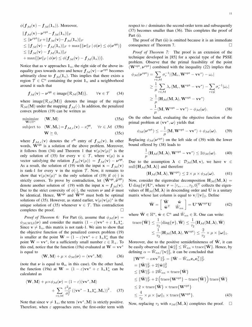
In order to demonstrate the efficacy of the proposed SDPproblem (15) in solving the power flow equations, we performnumerical simulations on the IEEE 9-bus, New England 39-bus, and IEEE 57-bus systems [87]. Three recovery methodsare considered for each test case:

1) Newton’s method: We evaluate the probability of conver-gence for Newton’s method in polar coordinates for theclassical PF problem with 2n− 1 specifications, wherethe starting point is vk = 1∠0◦ for every k ∈ N .

2) SDP relaxation: The probability of obtaining a rank-1solution for the SDP relaxation (15) with M = Y∗Yis evaluated, where the same set of specifications as inNewton’s method is used.

3) SDP relaxation with extra specifications: The probabilityof obtaining a rank-1 solution for the SDP relaxation(15) with M = Y∗Y is evaluated, under extra spec-ifications compared to the classical PF problem. It isassumed that active powers are measured at PV andPQ buses, reactive powers are measured at PQ buses,and voltages magnitudes are measured at all buses (asopposed to only PV and slack buses).

For different values of θ, we have generated 500 specificationsets (x1, . . . , x|M|) by randomly choosing voltage vectorswhose magnitudes and phases are uniformly drawn from theintervals [0.9, 1.1] and [−θ, θ], respectively. We have thenexploited each of the three methods described above to find afeasible voltage vector associated with each specification set.The results are depicted in Figure 1. It can be observed thatthe SDP relaxations outperform the Newton’s method.

B. Case Study: Power System State Estimation

In order to show that the penalized convex program (19)with a nonzero matrix M significantly outperforms the classi-cal SDP relaxation of PSSE proposed in [72]–[75], we conductsimulations on the PEGASE 1354-bus and 9241-bus systemsfrom [88]. Consider a positive number c. Suppose that allmeasurements are subject to zero mean Gaussian noises, wherethe standard deviations for squared voltage magnitude, nodalactive/reactive power, and branch flow measurements are c,1.5c and 2c times higher than the corresponding noiselessvalues of squared voltage magnitudes, nodal active/reactivepowers, and branch flows, respectively. Let M be equal toα× I−B, where the constant α is chosen in such a way thatα×I−B satisfies Assumption 2. This choice of M makes thefunction 〈M,W〉 account for the reactive loss in the network[41], [59].

We have performed simulations on the PEGASE 9241-bussystem with randomly generated noise values corresponding

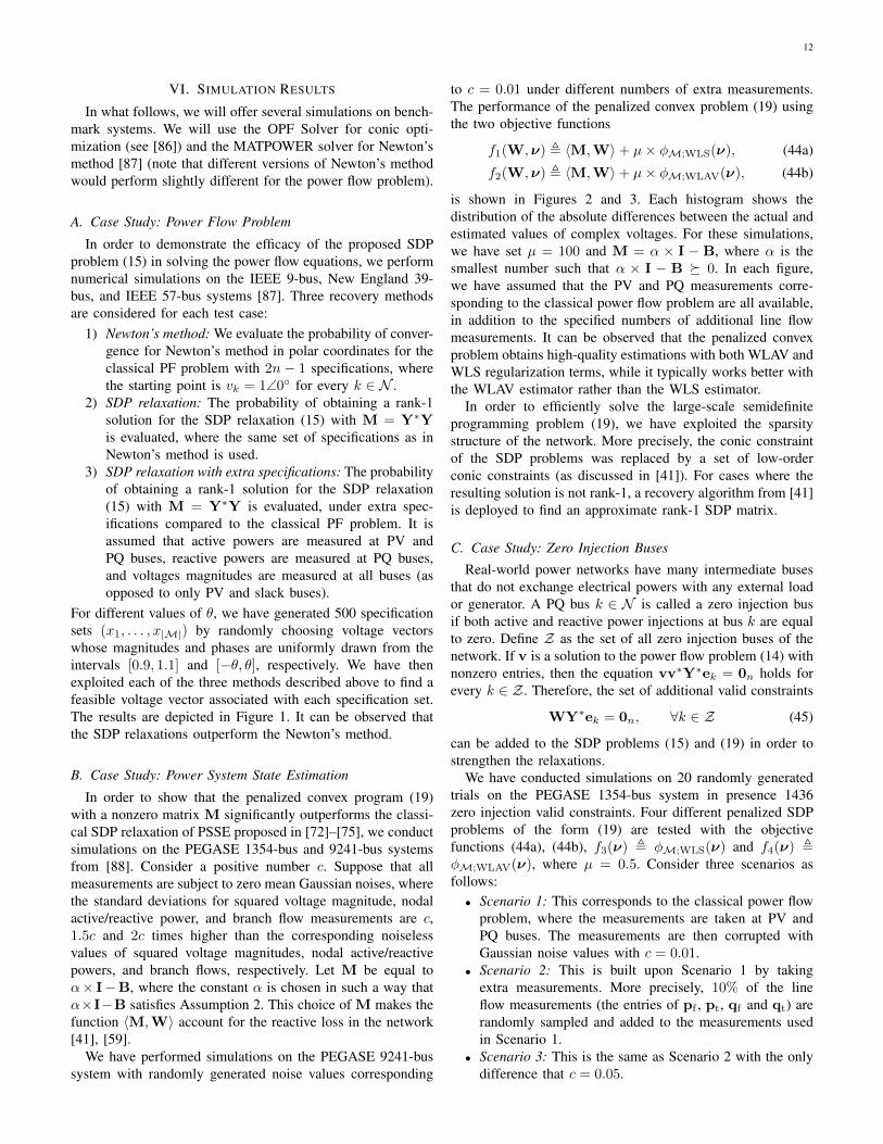
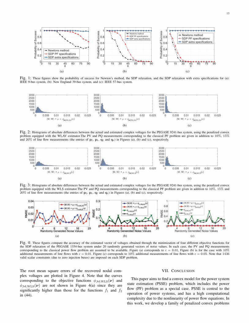
to c = 0.01 under different numbers of extra measurements.The performance of the penalized convex problem (19) usingthe two objective functions

f1(W,ν) , 〈M,W〉+ µ× φM;WLS(ν), (44a)

f2(W,ν) , 〈M,W〉+ µ× φM;WLAV(ν), (44b)

is shown in Figures 2 and 3. Each histogram shows thedistribution of the absolute differences between the actual andestimated values of complex voltages. For these simulations,we have set µ = 100 and M = α × I − B, where α is thesmallest number such that α × I − B � 0. In each figure,we have assumed that the PV and PQ measurements corre-sponding to the classical power flow problem are all available,in addition to the specified numbers of additional line flowmeasurements. It can be observed that the penalized convexproblem obtains high-quality estimations with both WLAV andWLS regularization terms, while it typically works better withthe WLAV estimator rather than the WLS estimator.

In order to efficiently solve the large-scale semidefiniteprogramming problem (19), we have exploited the sparsitystructure of the network. More precisely, the conic constraintof the SDP problems was replaced by a set of low-orderconic constraints (as discussed in [41]). For cases where theresulting solution is not rank-1, a recovery algorithm from [41]is deployed to find an approximate rank-1 SDP matrix.

C. Case Study: Zero Injection Buses

Real-world power networks have many intermediate busesthat do not exchange electrical powers with any external loador generator. A PQ bus k ∈ N is called a zero injection busif both active and reactive power injections at bus k are equalto zero. Define Z as the set of all zero injection buses of thenetwork. If v is a solution to the power flow problem (14) withnonzero entries, then the equation vv∗Y∗ek = 0n holds forevery k ∈ Z . Therefore, the set of additional valid constraints

WY∗ek = 0n, ∀k ∈ Z (45)

can be added to the SDP problems (15) and (19) in order tostrengthen the relaxations.

We have conducted simulations on 20 randomly generatedtrials on the PEGASE 1354-bus system in presence 1436zero injection valid constraints. Four different penalized SDPproblems of the form (19) are tested with the objectivefunctions (44a), (44b), f3(ν) , φM;WLS(ν) and f4(ν) ,φM;WLAV(ν), where µ = 0.5. Consider three scenarios asfollows:• Scenario 1: This corresponds to the classical power flow

problem, where the measurements are taken at PV andPQ buses. The measurements are then corrupted withGaussian noise values with c = 0.01.

• Scenario 2: This is built upon Scenario 1 by takingextra measurements. More precisely, 10% of the lineflow measurements (the entries of pf , pt, qf and qt) arerandomly sampled and added to the measurements usedin Scenario 1.

• Scenario 3: This is the same as Scenario 2 with the onlydifference that c = 0.05.

13

0 15 30 45 60 75 900

0.2

0.4

0.6

0.8

1

θ

Pro

babili

ty o

f S

uccess

Newtons method

SDP PF specifications

SDP extra s

(a)

0 15 30 45 60 75 900

0.2

0.4

0.6

0.8

1

θ

Pro

babili

ty o

f S

uccess

Newtons method


SDP extra specifications

(b)

0 15 30 45 60 75 900

0.2

0.4

0.6

0.8

1

θ

Pro

babili

ty o

f S

uccess

Newtons method


SDP extra specifications

(c)

Fig. 1: These figures show the probability of success for Newton’s method, the SDP relaxation, and the SDP relaxation with extra specifications for (a):IEEE 9-bus system, (b): New England 39-bus system, and (c): IEEE 57-bus system.

(a) (b) (c)

Fig. 2: Histograms of absolute differences between the actual and estimated complex voltages for the PEGASE 9241-bus system, using the penalized convexproblem equipped with the WLAV estimator.The PV and PQ measurements corresponding to the classical PF problem are given in addition to 10%, 15%and 20% of line flow measurements (the entries of pf , pt, qf and qt) in Figures (a), (b) and (c), respectively.

(a) (b) (c)

Fig. 3: Histograms of absolute differences between the actual and estimated complex voltages for the PEGASE 9241-bus system, using the penalized convexproblem equipped with the WLS estimator.The PV and PQ measurements corresponding to the classical PF problem are given in addition to 10%, 15% and20% of line flow measurements (the entries of pf , pt, qf and qt) in Figures (a), (b) and (c), respectively.

(a) (b) (c)

Fig. 4: These figures compare the accuracy of the estimated vector of voltages obtained through the minimization of four different objective functions forthe SDP relaxation of the PEGASE 1354-bus system under 20 randomly generated vectors of noise values. In each case, the PV and PQ measurementscorresponding to the classical power flow problem are assumed to be available. Figure (a) corresponds to c = 0.01, Figure (b) is for the case with 10%additional measurements of line flows with c = 0.01. Figure (c) corresponds to 10% additional measurements of line flows with c = 0.05. Note that 1436valid scalar constraints (due to zero injection buses) are imposed on each SDP problem.

The root mean square errors of the recovered nodal com-plex voltages are plotted in Figure 4. Note that the curvescorresponding to the objective functions φM;WLS(ν) andφM;WLS(ν) are not shown in Figure 4(a) since they aresignificantly higher than those for the functions f1 and f2in (44).

VII. CONCLUSION

This paper aims to find a convex model for the power systemstate estimation (PSSE) problem, which includes the powerflow (PF) problem as a special case. PSSE is central to theoperation of power systems, and has a high computationalcomplexity due to the nonlinearity of power flow equations. Inthis work, we develop a family of penalized convex problems

14

to solve the PSSE problem. It is shown that each convexprogram proposed in this paper finds the correct solution of thePSSE problem in the case of noiseless measurements, providedthat the voltage angles are relatively small. In presence ofnoisy measurements, it is proven that the penalized convexproblems are all able to find an approximate solution of thePSSE problem, where the estimation error has an explicitupper bound in terms of the power of the noise. The objectivefunction of each penalized convex problem has two terms: oneaccounting for the non-convexity of the power flow equationsand another one for estimating the noise level. Simulationresults on real-world systems elucidate the superiority of theproposed method in estimating the state of a power systembased on non-convex and noisy measurements.

ACKNOWLEDGEMENTS

The authors would like to thank Morteza Ashraphijuo forfruitful discussions on the simulation results of this paper.

REFERENCES

[1] A. Pinar, J. Meza, V. Donde, and B. Lesieutre, “Optimization strategiesfor the vulnerability analysis of the electric power grid,” SIAM Journalon Optimization, vol. 20, no. 4, pp. 1786–1810, 2010.

[2] A. Papavasiliou and S. S. Oren, “Multiarea stochastic unit commitmentfor high wind penetration in a transmission constrained network,”Operations Research, vol. 61, no. 3, pp. 578–592, 2013.

[3] D. Bienstock, M. Chertkov, and S. Harnett, “Chance-constrained optimalpower flow: Risk-aware network control under uncertainty,” SIAMReview, vol. 56, no. 3, pp. 461–495, 2014.

[4] B. Kocuk, H. Jeon, S. S. Dey, J. Linderoth, J. Luedtke, and X. A.Sun, “A cycle-based formulation and valid inequalities for DC powertransmission problems with switching,” Operations Research, 2016.

[5] K. Lehmann, A. Grastien, and P. V. Hentenryck, “AC-feasibility on treenetworks is NP-hard,” IEEE Transactions on Power Systems, vol. 31,no. 1, pp. 798–801, Jan 2016.

[6] A. Verma, “Power grid security analysis: An optimization approach,”Ph.D. dissertation, Columbia University, 2009.

[7] D. Bienstock and A. Verma, “Strong NP-hardness of AC power flowsfeasibility,” arXiv preprint arXiv:1512.07315, 2015.

[8] W. F. Tinney and C. E. Hart, “Power flow solution by Newton’s method,”IEEE Transactions on Power Systems, vol. 86, no. Nov., pp. 1449–1460,Jun. 1967.

[9] B. Stott and O. Alsac, “Fast decoupled load flow,” IEEE Transactionson Power Systems, vol. 93, no. 3, pp. 859–869, May. 1974.

[10] R. A. Van Amerongen, “A general-purpose version of the fast decoupledload flow,” IEEE Transactions on Power Systems, vol. 4, no. 2, pp. 760–770, May. 1989.

[11] D. Bienstock and G. Munoz, “On linear relaxations of OPF problems,”arXiv preprint arXiv:1411.1120, 2014.

[12] C. Coffrin and P. Van Hentenryck, “A linear-programming approxima-tion of AC power flows,” INFORMS Journal on Computing, vol. 26,no. 4, pp. 718–734, 2014.

[13] F. Salam, L. Ni, S. Guo, and X. Sun, “Parallel processing for the loadflow of power systems: the approach and applications,” in Proceedingsof the 28th IEEE Conference on Decision and Control, 1989, pp. 2173–2178.

[14] W. Ma and J. S. Thorp, “An efficient algorithm to locate all the loadflow solutions,” IEEE Transactions on Power Systems, vol. 8, no. 3, pp.1077–1083, 1993.

[15] C.-W. Liu, C.-S. Chang, J.-A. Jiang, and G.-H. Yeh, “Toward aCPFLOW-based algorithm to compute all the type-1 load-flow solutionsin electric power systems,” IEEE Transactions on Circuits and SystemsI: Regular Papers, vol. 52, no. 3, pp. 625–630, 2005.

[16] D. K. Molzahn, B. C. Lesieutre, and H. Chen, “Counterexample to acontinuation-based algorithm for finding all power flow solutions,” IEEETransactions on Power Systems, vol. 28, no. 1, pp. 564–565, 2013.

[17] D. Mehta, H. Nguyen, and K. Turitsyn, “Numerical polynomial homo-topy continuation method to locate all the power flow solutions,” arXivpreprint arXiv:1408.2732, 2014.

[18] S. Chandra, D. Mehta, and A. Chakrabortty, “Equilibria analysis ofpower systems using a numerical homotopy method,” in IEEE Power &Energy Society General Meeting, 2015, pp. 1–5.

[19] A. Montes and J. Castro, “Solving the load flow problem using Groebnerbasis,” ACM SIGSAM Bulletin, vol. 29, no. 1, pp. 1–13, 1995.

[20] J. Ning, W. Gao, G. Radman, and J. Liu, “The application of theGroebner basis technique in power flow study,” in North AmericanPower Symposium (NAPS), 2009, pp. 1–7.

[21] H. Mori and A. Yuihara, “Calculation of multiple power flow solutionswith the Krawczyk method,” in Proceedings of the 1999 IEEE Interna-tional Symposium on Circuits and Systems, vol. 5, 1999, pp. 94–97.

[22] D. K. Molzahn, D. Mehta, and M. Niemerg, “Toward topologically basedupper bounds on the number of power flow solutions,” arXiv preprintarXiv:1509.09227, 2015.

[23] T. Chen and D. Mehta, “On the network topology dependent so-lution count of the algebraic load flow equations,” arXiv preprintarXiv:1512.04987, 2015.

[24] L. Vandenberghe and S. Boyd, “Semidefinite programming,” SIAMreview, vol. 38, no. 1, pp. 49–95, 1996.

[25] F. Alizadeh, “Interior point methods in semidefinite programming withapplications to combinatorial optimization,” SIAM Journal on Optimiza-tion, vol. 5, no. 1, pp. 13–51, 1995.

[26] F. Alizadeh, J.-P. A. Haeberly, and M. L. Overton, “Complementarityand nondegeneracy in semidefinite programming,” Mathematical Pro-gramming, vol. 77, no. 1, pp. 111–128, 1997.

[27] Z. Li, S. He, and S. Zhang, Approximation methods for polynomialoptimization: Models, Algorithms, and Applications. Springer Science& Business Media, 2012.

[28] M. X. Goemans and D. P. Williamson, “Improved approximation algo-rithms for maximum cut and satisfiability problems using semidefiniteprogramming,” Journal of the ACM (JACM), vol. 42, no. 6, pp. 1115–1145, 1995.

[29] S. Sojoudi and J. Lavaei, “Exactness of semidefinite relaxations fornonlinear optimization problems with underlying graph structure,” SIAMJournal on Optimization, vol. 24, no. 4, pp. 1746–1778, 2014.

[30] Y. Nesterov, “Semidefinite relaxation and nonconvex quadratic optimiza-tion,” Optimization methods and software, vol. 9, no. 1-3, pp. 141–160,1998.

[31] S. Zhang and Y. Huang, “Complex quadratic optimization and semidef-inite programming,” SIAM Journal on Optimization, vol. 16, no. 3, pp.871–890, 2006.

[32] Z.-Q. Luo and S. Zhang, “A semidefinite relaxation scheme for mul-tivariate quartic polynomial optimization with quadratic constraints,”SIAM Journal on Optimization, vol. 20, no. 4, pp. 1716–1736, 2010.

[33] A. Beck, Y. Drori, and M. Teboulle, “A new semidefinite programmingrelaxation scheme for a class of quadratic matrix problems,” OperationsResearch Letters, vol. 40, no. 4, pp. 298–302, 2012.

[34] B. Jiang, Z. Li, and S. Zhang, “Approximation methods for complexpolynomial optimization,” Computational Optimization and Applica-tions, vol. 59, no. 1-2, pp. 219–248, 2014.

[35] S. He, Z. Li, and S. Zhang, “Approximation algorithms for discretepolynomial optimization,” Journal of the Operations Research Societyof China, vol. 1, no. 1, pp. 3–36, 2013.

[36] S. He, Z. Li, and S. Zhang, “Approximation algorithms for homogeneouspolynomial optimization with quadratic constraints,” Mathematical Pro-gramming, vol. 125, no. 2, pp. 353–383, 2010.

[37] Y. Huang, A. De Maio, and S. Zhang, “Semidefinite programming,matrix decomposition, and radar code design,” Convex Optimization inSignal Processing and Communications, pp. 192–228, 2010.

[38] Y. Huang and S. Zhang, “Approximation algorithms for indefinite com-plex quadratic maximization problems,” Science China Mathematics,vol. 53, no. 10, pp. 2697–2708, 2010.

[39] S. He, Z.-Q. Luo, J. Nie, and S. Zhang, “Semidefinite relaxation boundsfor indefinite homogeneous quadratic optimization,” SIAM Journal onOptimization, vol. 19, no. 2, pp. 503–523, 2008.

[40] Z.-Q. Luo, N. D. Sidiropoulos, P. Tseng, and S. Zhang, “Approximationbounds for quadratic optimization with homogeneous quadratic con-straints,” SIAM Journal on optimization, vol. 18, no. 1, pp. 1–28, 2007.

[41] R. Madani, M. Ashraphijuo, and J. Lavaei, “Promises of conic relax-ation for contingency-constrained optimal power flow problem,” IEEETransactions on Power Systems, vol. 31, no. 2, pp. 1297–1307, March2016.

[42] R. Madani, G. Fazelnia, S. Sojoudi, and J. Lavaei, “Low-rank solutionsof matrix inequalities with applications to polynomial optimizationand matrix completion problems,” in Proceedings of the 53rd IEEEConference on Decision and Control, 2014.

15

[43] P. A. Parrilo, “Structured semidefinite programs and semialgebraicgeometry methods in robustness and optimization,” Ph.D. dissertation,2000.

[44] A. Beck and M. Teboulle, “Global optimality conditions for quadraticoptimization problems with binary constraints,” SIAM Journal on Opti-mization, vol. 11, no. 1, pp. 179–188, 2000.

[45] S. Prajna, A. Papachristodoulou, P. Seiler, and P. A. Parrilo, “Newdevelopments in sum of squares optimization and SOSTOOLS,” inProceedings of the American Control Conference, 2004, pp. 5606–5611.

[46] J. B. Lasserre, “Global optimization with polynomials and the problemof moments,” SIAM Journal on Optimization, vol. 11, no. 3, pp. 796–817, 2001.

[47] J. F. Bonnans, “Mathematical study of very high voltage power networksI: The optimal DC power flow problem,” SIAM Journal on Optimization,vol. 7, no. 4, pp. 979–990, 1997.

[48] J. F. Bonnans, “Mathematical study of very high voltage power networksII: The AC power flow problem,” SIAM Journal on Applied Mathemat-ics, vol. 58, no. 5, pp. 1547–1567, 1998.

[49] J. Thorp and S. Naqavi, “Load flow fractals,” in Proceedings of the 28thIEEE Conference on Decision and Control, 1989, pp. 1822–1827.

[50] A. Abur and A. G. Exposito, Power system state estimation: theory andimplementation. CRC press, 2004.

[51] E. J. Candes, Y. C. Eldar, T. Strohmer, and V. Voroninski, “Phaseretrieval via matrix completion,” SIAM Review, vol. 57, no. 2, pp. 225–251, 2015.

[52] J. Lavaei, “Zero duality gap for classical OPF problem convexifiesfundamental nonlinear power problems,” in Proceedings of the AmericanControl Conference, June 2011, pp. 4566–4573.

[53] J. Lavaei and S. Low, “Zero duality gap in optimal power flow problem,”IEEE Transactions on Power Systems, vol. 27, no. 1, pp. 92–107, Feb.2012.

[54] S. Sojoudi and J. Lavaei, “Physics of power networks makes hardoptimization problems easy to solve,” in IEEE Power and Energy SocietyGeneral Meeting, 2012, pp. 1–8.

[55] D. T. Phan, “Lagrangian duality and branch-and-bound algorithms foroptimal power flow,” Operations Research, vol. 60, no. 2, pp. 275–285,2012.

[56] C. Chen, A. Atamturk, and S. S. Oren, “Bound tightening for thealternating current optimal power flow problem,” IEEE Transactions onPower Systems, vol. PP, no. 99, pp. 1–8, 2015.

[57] B. Kocuk, S. S. Dey, and X. A. Sun, “Inexactness of SDP relaxationand valid inequalities for optimal power flow,” IEEE Transactions onPower Systems, vol. 31, no. 1, pp. 642–651, 2016.

[58] C. Coffrin, H. Hijazi, and P. Van Hentenryck, “Strengthening the SDPrelaxation of AC power flows with convex envelopes, bound tightening,and lifted nonlinear cuts,” arXiv preprint arXiv:1512.04644, 2015.

[59] R. Madani, S. Sojoudi, and J. Lavaei, “Convex relaxation for optimalpower flow problem: Mesh networks,” IEEE Transactions on PowerSystems, vol. 30, no. 1, pp. 199–211, Jan. 2015.

[60] D. Bienstock and G. Munoz, “LP approximations to mixed-integerpolynomial optimization problems,” arXiv preprint arXiv:1501.00288,2015.

[61] M. Fukuda, M. Kojima, K. Murota, and K. Nakata, “Exploiting sparsityin semidefinite programming via matrix completion I: General frame-work,” SIAM Journal on Optimization, vol. 11, no. 3, pp. 647–674,2001.

[62] K. Nakata, K. Fujisawa, M. Fukuda, M. Kojima, and K. Murota,“Exploiting sparsity in semidefinite programming via matrix completionII: Implementation and numerical results,” Mathematical Programming,vol. 95, no. 2, pp. 303–327, 2003.

[63] A. Lam, B. Zhang, and D. Tse, “Distributed algorithms for optimalpower flow problem,” in Proceedings of the 51st IEEE Conference onDecision and Control, 2012.

[64] B. Zhang, A. Y. S. Lam, A. D. Domnguez-Garca, and D. Tse, “Anoptimal and distributed method for voltage regulation in power distri-bution systems,” IEEE Transactions on Power Systems, vol. 30, no. 4,pp. 1714–1726, July 2015.

[65] D. K. Molzahn, J. T. Holzer, B. C. Lesieutre, and C. L. DeMarco,“Implementation of a large-scale optimal power flow solver basedon semidefinite programming,” IEEE Transactions on Power Systems,vol. 28, no. 4, pp. 3987–3998, Nov. 2013.

[66] M. S. Andersen, A. Hansson, and L. Vandenberghe, “Reduced-complexity semidefinite relaxations of optimal power flow problems,”IEEE Transactions on Power Systems, vol. 29, no. 4, pp. 1855–1863,Jul 2014.

[67] R. Jabr, “Exploiting sparsity in SDP relaxations of the OPF problem,”IEEE Transactions on Power Systems, vol. 27, no. 2, pp. 1138–1139,May. 2012.

[68] B. Kocuk, S. S. Dey, and X. A. Sun, “Strong SOCP relaxations for theoptimal power flow problem,” Operations Research, 2016.

[69] B. Kocuk, S. S. Dey, and X. A. Sun, “New formulation and strongMISOCP relaxations for AC optimal transmission switching problem,”arXiv preprint arXiv:1510.02064, 2015.

[70] S. H. Low, “Convex relaxation of optimal power flow–Part I: Formu-lations and equivalence,” IEEE Transactions on Control of NetworkSystems, vol. 1, no. 1, pp. 15–27, 2014.

[71] S. H. Low, “Convex relaxation of optimal power flow–Part II: Exact-ness,” IEEE Transactions on Control of Network Systems, vol. 1, no. 2,pp. 177–189, 2014.

[72] H. Zhu and G. Giannakis, “Power system nonlinear state estimationusing distributed semidefinite programming,” IEEE Journal of SelectedTopics in Signal Processing, vol. 8, no. 6, pp. 1039–1050, 2014.

[73] Y. Weng, Q. Li, R. Negi, and M. Ilic, “Distributed algorithm for SDPstate estimation,” in Proceedings of the 2013 IEEE PES Innovative SmartGrid Technologies (ISGT), 2013, pp. 1–6.

[74] Y. Weng, M. D. Ilic, Q. Li, and R. Negi, “Convexification of bad dataand topology error detection and identification problems in AC electricpower systems,” IET Generation, Transmission & Distribution, vol. 9,no. 16, pp. 2760–2767, Nov 2015.

[75] Y. Weng, Q. Li, R. Negi, and M. Ilic, “Semidefinite programming forpower system state estimation,” in IEEE Power and Energy SocietyGeneral Meeting, July 2012, pp. 1–8.

[76] A. Beck and Y. C. Eldar, “Sparsity constrained nonlinear optimization:Optimality conditions and algorithms,” SIAM Journal on Optimization,vol. 23, no. 3, pp. 1480–1509, 2013.

[77] A. Beck, Y. C. Eldar, and Y. Shechtman, “Nonlinear compressed sensingwith application to phase retrieval,” in Global Conference on Signal andInformation Processing, 2013, pp. 617–617.

[78] Y. Chen and E. Candes, “Solving random quadratic systems of equationsis nearly as easy as solving linear systems,” in Advances in NeuralInformation Processing Systems, 2015, pp. 739–747.

[79] E. J. Candes, X. Li, and M. Soltanolkotabi, “Phase retrieval via Wirtingerflow: Theory and algorithms,” IEEE Transactions on Information The-ory, vol. 61, no. 4, pp. 1985–2007, 2015.

[80] E. J. Candes, T. Strohmer, and V. Voroninski, “Phaselift: Exact andstable signal recovery from magnitude measurements via convex pro-gramming,” Communications on Pure and Applied Mathematics, vol. 66,no. 8, pp. 1241–1274, Aug. 2013.

[81] B. Recht, M. Fazel, and P. A. Parrilo, “Guaranteed minimum-ranksolutions of linear matrix equations via nuclear norm minimization,”SIAM Rev., vol. 52, no. 3, pp. 471–501, Aug. 2010.

[82] W. Ai, Y. Huang, and S. Zhang, “On the low rank solutions for linearmatrix inequalities,” Mathematics of Operations Research, vol. 33, no. 4,pp. 965–975, 2008.

[83] R. Madani, J. Lavaei, and R. Baldick, “Convexification of power flowproblem over arbitrary networks,” in 54th IEEE Conference on Decisionand Control, 2015, pp. 1–8.

[84] A. Duval, C. Klivans, and J. Martin, “Simplicial matrix-tree theorems,”T. Am. Math. Soc., vol. 361, no. 11, pp. 6073–6114, Jun. 2009.

[85] Y. Zhang, R. Madani, and J. Lavaei, “Power system state estimationwith line measurements,” in Decision and Control (CDC), 2016 IEEE55th Conference on. IEEE, 2016, pp. 2403–2410.

[86] R. Madani, M. Ashraphijuo, and J. Lavaei, “OPF Solver,” http:// ieor.berkeley.edu/∼lavaei/Software.html, 2014.

[87] R. D. Zimmerman, C. E. Murillo-Sanchez, and R. J. Thomas, “Mat-power’s extensible optimal power flow architecture,” in IEEE Power &Energy Society General Meeting, 2009, pp. 1–7.

[88] S. Fliscounakis, P. Panciatici, F. Capitanescu, and L. Wehenkel, “Con-tingency ranking with respect to overloads in very large power systemstaking into account uncertainty, preventive, and corrective actions,” IEEETransactions on Power Systems, vol. 28, no. 4, pp. 4909–4917, 2013.

http://ieor.berkeley.edu/~lavaei/Software.html

http://ieor.berkeley.edu/~lavaei/Software.html

16

Ramtin Madani is an Assistant Professor at theElectrical Engineering Department of the Universityof Texas at Arlington. He received the Ph.D. degreein Electrical Engineering from Columbia Universityin 2015, and was a postdoctoral scholar in the De-partment of Industrial Engineering and OperationsResearch at University of California, Berkeley in2016.

Javad Lavaei is an Assistant Professor in the De-partment of Industrial Engineering and OperationsResearch at University of California, Berkeley. Heobtained his Ph.D. degree in Computing and Math-ematical Sciences from California Institute of Tech-nology in 2011. He has won multiple awards, includ-ing NSF CAREER Award, Office of Naval ResearchYoung Investigator Award, AFOSR Young FacultyAward, DARPA Young Faculty Award, Google Fac-ulty Research Award, Donald P. Eckman Award,Resonate Award, INFORMS Optimization Society

Prize for Young Researchers, INFORMS ENRE Energy Best PublicationAward, and SIAM Control and Systems Theory Prize.

Ross Baldick (F07) received the B.Sc. degree inmathematics and physics and the B.E. degree inelectrical engineering from the University of Sydney,Sydney, Australia, and the M.S. and Ph.D. degreesin electrical engineering and computer sciences fromthe University of California, Berkeley, in 1988 and1990, respectively. From 1991 to 1992, he was aPost-Doctoral Fellow with the Lawrence BerkeleyLaboratory, Berkeley, CA. In 1992 and 1993, hewas an Assistant Professor with the Worcester Poly-technic Institute, Worcester, MA. He is currently

a Professor with the Department of Electrical and Computer Engineering,University of Texas, Austin.

Date post:	16-May-2018
Category:	Documents
Upload:	trinhdieu
View:	227 times
Download:	3 times

Convexiﬁcation of Power Flow Equations for Power …lavaei/SE_J_2016.pdf · Convexiﬁcation of...

Documents